local null controllability of the three-dimensional … · outline presentation algebraic...
TRANSCRIPT
Outline Presentation Algebraic resolution Application to Navier-Stokes Perspectives
Local null controllability of the three-dimensionalNavier-Stokes system with a distributed control
having two vanishing componentsjoint work with Jean-Michel Coron
Pierre Lissy
Laboratoire Jacques-Louis Lions, Université Pierre et Marie Curie
Partial dierential equations, optimal design and numerics,
Benasque
August 29, 2013
Pierre Lissy Laboratoire Jacques-Louis Lions, Université Pierre et Marie Curie
Controllability of Navier-Stokes 3D with a scalar control

Outline Presentation Algebraic resolution Application to Navier-Stokes Perspectives
Outline
Presentation of the problem
Introduction
The linearized system
The particular trajectory
Algebraic resolution of dierential systems
Some notations and general ideas
A simple example
Application to the controllability of Navier-Stokes equations
Algebraic solvability and its link with controllability
How to ndMRegular controls of a particular form
Perspectives
Pierre Lissy Laboratoire Jacques-Louis Lions, Université Pierre et Marie Curie
Controllability of Navier-Stokes 3D with a scalar control
Outline Presentation Algebraic resolution Application to Navier-Stokes Perspectives
Introduction
Presentation of the problem
Introduction
The linearized system
The particular trajectory
Algebraic resolution of dierential systems
Some notations and general ideas
A simple example
Application to the controllability of Navier-Stokes equations
Algebraic solvability and its link with controllability
How to ndMRegular controls of a particular form
PerspectivesPierre Lissy Laboratoire Jacques-Louis Lions, Université Pierre et Marie Curie
Controllability of Navier-Stokes 3D with a scalar control
Outline Presentation Algebraic resolution Application to Navier-Stokes Perspectives
Introduction
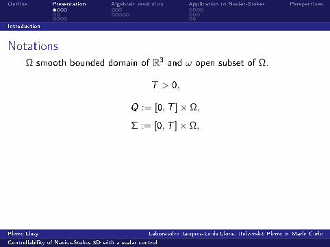
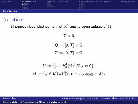
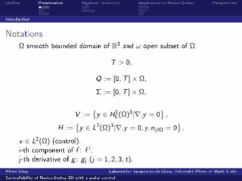
NotationsΩ smooth bounded domain of R3 and ω open subset of Ω.
T > 0,
Q := [0,T ]× Ω,
Σ := [0,T ]× Ω,
V :=y ∈ H1
0 (Ω)3|∇.y = 0,
H :=y ∈ L2(Ω)3|∇.y = 0, y .n|∂Ω = 0
.
v ∈ L2(Ω) (control).
i-th component of f : f i .
j-th derivative of g : gj (j = 1, 2, 3, t).
Pierre Lissy Laboratoire Jacques-Louis Lions, Université Pierre et Marie Curie
Controllability of Navier-Stokes 3D with a scalar control
Outline Presentation Algebraic resolution Application to Navier-Stokes Perspectives
Introduction
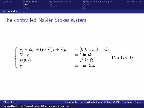
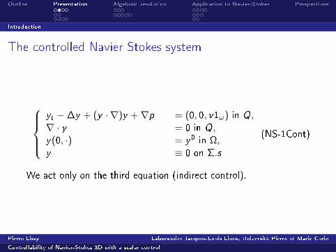
The controlled Navier-Stokes system
yt −∆y + (y · ∇)y +∇p = (0, 0, v1ω) in Q,∇ · y = 0 in Q,y(0, ·) = y0 in Ω,y ≡ 0 on Σ.s
(NS-1Cont)
We act only on the third equation (indirect control).
Pierre Lissy Laboratoire Jacques-Louis Lions, Université Pierre et Marie Curie
Controllability of Navier-Stokes 3D with a scalar control
Outline Presentation Algebraic resolution Application to Navier-Stokes Perspectives
Introduction
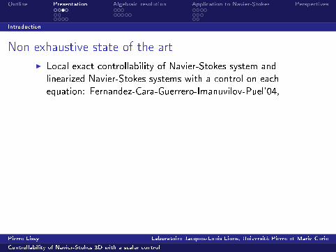
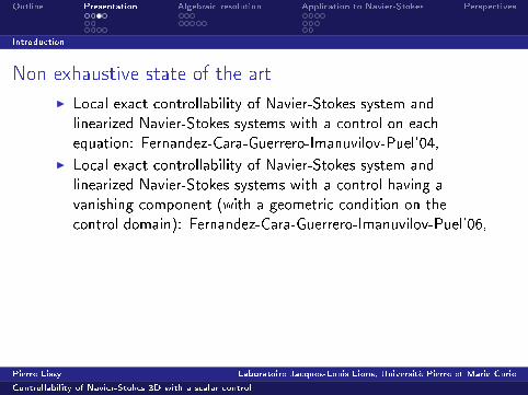
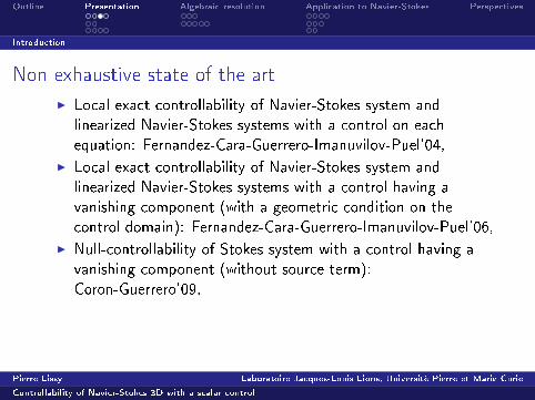
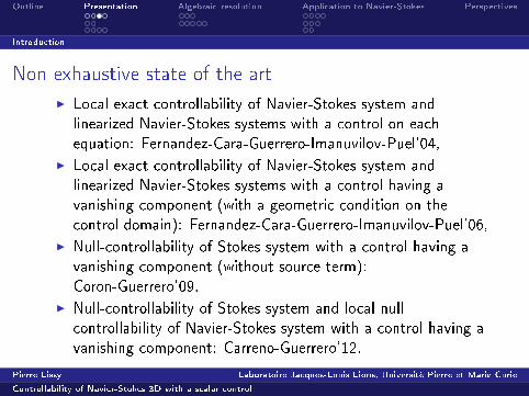
Non-exhaustive state of the art
I Local exact controllability of Navier-Stokes system and
linearized Navier-Stokes systems with a control on each
equation: Fernandez-Cara-Guerrero-Imanuvilov-Puel'04,
I Local exact controllability of Navier-Stokes system and
linearized Navier-Stokes systems with a control having a
vanishing component (with a geometric condition on the
control domain): Fernandez-Cara-Guerrero-Imanuvilov-Puel'06,
I Null-controllability of Stokes system with a control having a
vanishing component (without source term):
Coron-Guerrero'09,
I Null-controllability of Stokes system and local null
controllability of Navier-Stokes system with a control having a
vanishing component: Carreno-Guerrero'12.
Pierre Lissy Laboratoire Jacques-Louis Lions, Université Pierre et Marie Curie
Controllability of Navier-Stokes 3D with a scalar control
Outline Presentation Algebraic resolution Application to Navier-Stokes Perspectives
Introduction
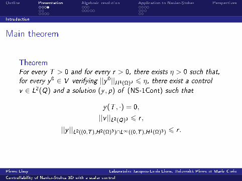
Main theorem
TheoremFor every T > 0 and for every r > 0, there exists η > 0 such that,
for every y0 ∈ V verifying ||y0||H1(Ω)3 6 η, there exist a control
v ∈ L2(Q) and a solution (y , p) of (NS-1Cont) such that
y(T , ·) = 0,
||v ||L2(Q)3 6 r ,
||y ||L2((0,T ),H2(Ω)3)∩L∞((0,T ),H1(Ω)3) 6 r .
Pierre Lissy Laboratoire Jacques-Louis Lions, Université Pierre et Marie Curie
Controllability of Navier-Stokes 3D with a scalar control
Outline Presentation Algebraic resolution Application to Navier-Stokes Perspectives
The linearized system
Presentation of the problem
Introduction
The linearized system
The particular trajectory
Algebraic resolution of dierential systems
Some notations and general ideas
A simple example
Application to the controllability of Navier-Stokes equations
Algebraic solvability and its link with controllability
How to ndMRegular controls of a particular form
PerspectivesPierre Lissy Laboratoire Jacques-Louis Lions, Université Pierre et Marie Curie
Controllability of Navier-Stokes 3D with a scalar control
Outline Presentation Algebraic resolution Application to Navier-Stokes Perspectives
The linearized system
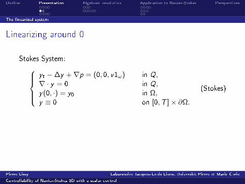
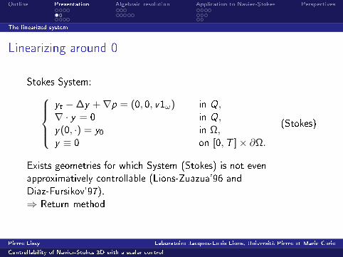
Linearizing around 0
Stokes System:
yt −∆y +∇p = (0, 0, v1ω) in Q,∇ · y = 0 in Q,y(0, ·) = y0 in Ω,y ≡ 0 on [0,T ]× ∂Ω.
(Stokes)
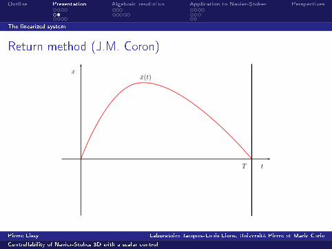
Exists geometries for which System (Stokes) is not even
approximatively controllable (Lions-Zuazua'96 and
Diaz-Fursikov'97).
⇒ Return method
Pierre Lissy Laboratoire Jacques-Louis Lions, Université Pierre et Marie Curie
Controllability of Navier-Stokes 3D with a scalar control
Outline Presentation Algebraic resolution Application to Navier-Stokes Perspectives
The linearized system
Linearizing around 0
Stokes System:yt −∆y +∇p = (0, 0, v1ω) in Q,∇ · y = 0 in Q,y(0, ·) = y0 in Ω,y ≡ 0 on [0,T ]× ∂Ω.
(Stokes)
Exists geometries for which System (Stokes) is not even
approximatively controllable (Lions-Zuazua'96 and
Diaz-Fursikov'97).
⇒ Return method
Pierre Lissy Laboratoire Jacques-Louis Lions, Université Pierre et Marie Curie
Controllability of Navier-Stokes 3D with a scalar control

Outline Presentation Algebraic resolution Application to Navier-Stokes Perspectives
The linearized system
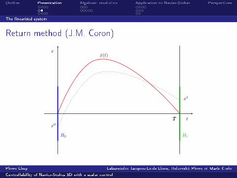
Return method (J.M. Coron)
T
x
t
2
Pierre Lissy Laboratoire Jacques-Louis Lions, Université Pierre et Marie Curie
Controllability of Navier-Stokes 3D with a scalar control
Outline Presentation Algebraic resolution Application to Navier-Stokes Perspectives
The linearized system
Return method (J.M. Coron)
T
x
t
x(t)
3
Pierre Lissy Laboratoire Jacques-Louis Lions, Université Pierre et Marie Curie
Controllability of Navier-Stokes 3D with a scalar control
Outline Presentation Algebraic resolution Application to Navier-Stokes Perspectives
The linearized system
Return method (J.M. Coron)
T
x
tT
x0
x1
B0 B1
x(t)
4
Pierre Lissy Laboratoire Jacques-Louis Lions, Université Pierre et Marie Curie
Controllability of Navier-Stokes 3D with a scalar control
Outline Presentation Algebraic resolution Application to Navier-Stokes Perspectives
The linearized system
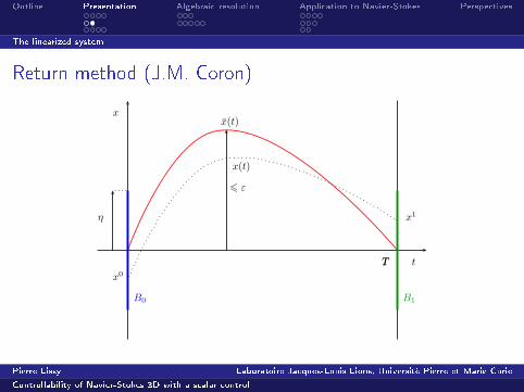
Return method (J.M. Coron)
T
x
tT
η
6 ε
x(t)
x(t)
x0
x1
B0 B1
5
Pierre Lissy Laboratoire Jacques-Louis Lions, Université Pierre et Marie Curie
Controllability of Navier-Stokes 3D with a scalar control
Outline Presentation Algebraic resolution Application to Navier-Stokes Perspectives
The particular trajectory
Presentation of the problem
Introduction
The linearized system
The particular trajectory
Algebraic resolution of dierential systems
Some notations and general ideas
A simple example
Application to the controllability of Navier-Stokes equations
Algebraic solvability and its link with controllability
How to ndMRegular controls of a particular form
PerspectivesPierre Lissy Laboratoire Jacques-Louis Lions, Université Pierre et Marie Curie
Controllability of Navier-Stokes 3D with a scalar control

Outline Presentation Algebraic resolution Application to Navier-Stokes Perspectives
The particular trajectory
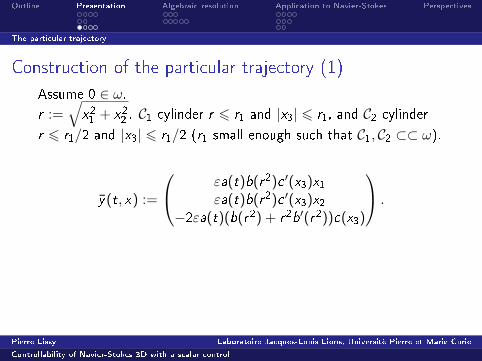
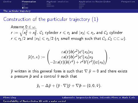
Construction of the particular trajectory (1)
Assume 0 ∈ ω.r :=
√x21 + x22 . C1 cylinder r 6 r1 and |x3| 6 r1, and C2 cylinder
r 6 r1/2 and |x3| 6 r1/2 (r1 small enough such that C1, C2 ⊂⊂ ω).
y(t, x) :=
εa(t)b(r2)c ′(x3)x1εa(t)b(r2)c ′(x3)x2
−2εa(t)(b(r2) + r2b′(r2))c(x3)
.
y written in this general form is such that ∇.y = 0 and there exists
a pressure p and a control v such that
yt −∆y + (y · ∇)y +∇p = (0, 0, v).
Pierre Lissy Laboratoire Jacques-Louis Lions, Université Pierre et Marie Curie
Controllability of Navier-Stokes 3D with a scalar control
Outline Presentation Algebraic resolution Application to Navier-Stokes Perspectives
The particular trajectory
Construction of the particular trajectory (2)
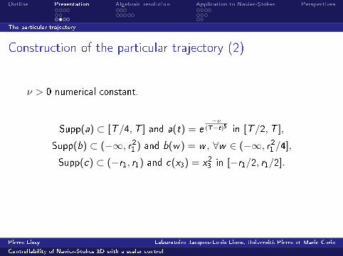
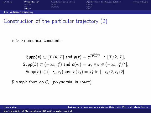
ν > 0 numerical constant.
Supp(a) ⊂ [T/4,T ] and a(t) = e−ν
(T−t)5 in [T/2,T ],
Supp(b) ⊂ (−∞, r21 ) and b(w) = w , ∀w ∈ (−∞, r21 /4],
Supp(c) ⊂ (−r1, r1) and c(x3) = x23 in [−r1/2, r1/2].
y simple form on C2 (polynomial in space).
Pierre Lissy Laboratoire Jacques-Louis Lions, Université Pierre et Marie Curie
Controllability of Navier-Stokes 3D with a scalar control
Outline Presentation Algebraic resolution Application to Navier-Stokes Perspectives
The particular trajectory
Construction of the particular trajectory (2)
ν > 0 numerical constant.
Supp(a) ⊂ [T/4,T ] and a(t) = e−ν
(T−t)5 in [T/2,T ],
Supp(b) ⊂ (−∞, r21 ) and b(w) = w , ∀w ∈ (−∞, r21 /4],
Supp(c) ⊂ (−r1, r1) and c(x3) = x23 in [−r1/2, r1/2].
y simple form on C2 (polynomial in space).
Pierre Lissy Laboratoire Jacques-Louis Lions, Université Pierre et Marie Curie
Controllability of Navier-Stokes 3D with a scalar control
Outline Presentation Algebraic resolution Application to Navier-Stokes Perspectives
The particular trajectory
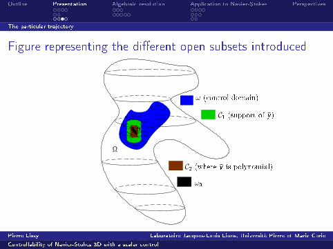
Figure representing the dierent open subsets introduced
0
Ω
C1 (support of y)
C2 (where y is polynomial)
ω (control domain)
ω0
Figure : The open subsets C1, C2, ω0, ω.Pierre Lissy Laboratoire Jacques-Louis Lions, Université Pierre et Marie Curie
Controllability of Navier-Stokes 3D with a scalar control
Outline Presentation Algebraic resolution Application to Navier-Stokes Perspectives
The particular trajectory
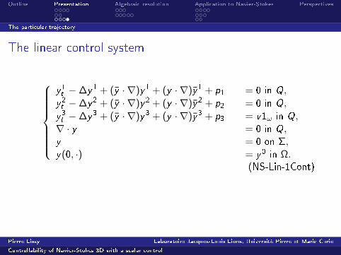
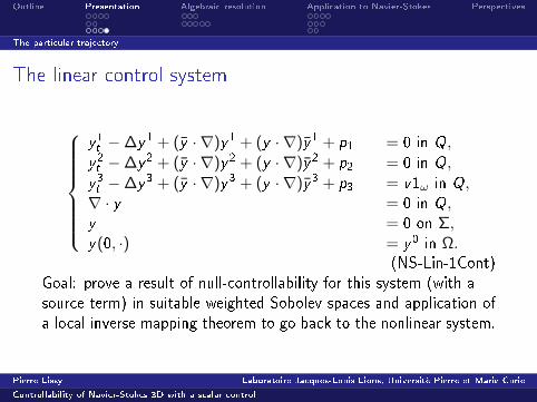
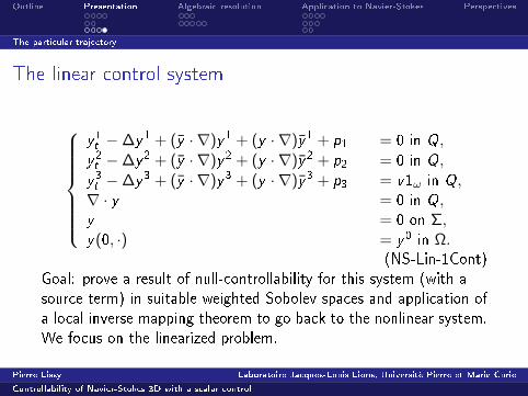
The linear control system
y1t −∆y1 + (y · ∇)y1 + (y · ∇)y1 + p1 = 0 in Q,
y2t −∆y2 + (y · ∇)y2 + (y · ∇)y2 + p2 = 0 in Q,
y3t −∆y3 + (y · ∇)y3 + (y · ∇)y3 + p3 = v1ω in Q,∇ · y = 0 in Q,y = 0 on Σ,y(0, ·) = y0 in Ω.
(NS-Lin-1Cont)
Goal: prove a result of null-controllability for this system (with a
source term) in suitable weighted Sobolev spaces and application of
a local inverse mapping theorem to go back to the nonlinear system.
We focus on the linearized problem.
Pierre Lissy Laboratoire Jacques-Louis Lions, Université Pierre et Marie Curie
Controllability of Navier-Stokes 3D with a scalar control
Outline Presentation Algebraic resolution Application to Navier-Stokes Perspectives
The particular trajectory
The linear control system
y1t −∆y1 + (y · ∇)y1 + (y · ∇)y1 + p1 = 0 in Q,
y2t −∆y2 + (y · ∇)y2 + (y · ∇)y2 + p2 = 0 in Q,
y3t −∆y3 + (y · ∇)y3 + (y · ∇)y3 + p3 = v1ω in Q,∇ · y = 0 in Q,y = 0 on Σ,y(0, ·) = y0 in Ω.
(NS-Lin-1Cont)
Goal: prove a result of null-controllability for this system (with a
source term) in suitable weighted Sobolev spaces and application of
a local inverse mapping theorem to go back to the nonlinear system.
We focus on the linearized problem.
Pierre Lissy Laboratoire Jacques-Louis Lions, Université Pierre et Marie Curie
Controllability of Navier-Stokes 3D with a scalar control
Outline Presentation Algebraic resolution Application to Navier-Stokes Perspectives
Some notations and general ideas
Presentation of the problem
Introduction
The linearized system
The particular trajectory
Algebraic resolution of dierential systems
Some notations and general ideas
A simple example
Application to the controllability of Navier-Stokes equations
Algebraic solvability and its link with controllability
How to ndMRegular controls of a particular form
PerspectivesPierre Lissy Laboratoire Jacques-Louis Lions, Université Pierre et Marie Curie
Controllability of Navier-Stokes 3D with a scalar control
Outline Presentation Algebraic resolution Application to Navier-Stokes Perspectives
Some notations and general ideas
Dierential operators
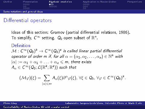
Ideas of this section: Gromov (partial dierential relations, 1986).
To simplify, C∞ setting. Q0 open subset of Rn.
DenitionM : C∞(Q0)k → C∞(Q0)s is called linear partial dierential
operator of order m if, for all α = (α1, α2, . . . , αn) ∈ Nn with
|α| := α1 + α1 + . . .+ αn 6 m, there exists
Aα ∈ C∞(Q0;L(Rk ;Rs)) such that
(Mϕ)(ξ) =∑|α|6m
Aα(ξ)∂αϕ(ξ), ∀ξ ∈ Q0, ∀ϕ ∈ C∞(Q0)k .
Pierre Lissy Laboratoire Jacques-Louis Lions, Université Pierre et Marie Curie
Controllability of Navier-Stokes 3D with a scalar control
Outline Presentation Algebraic resolution Application to Navier-Stokes Perspectives
Some notations and general ideas
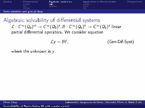
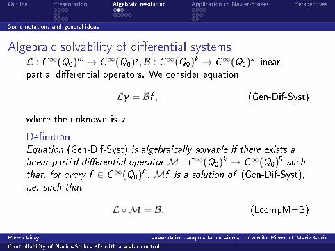
Algebraic solvability of dierential systemsL : C∞(Q0)m → C∞(Q0)s ,B : C∞(Q0)k → C∞(Q0)s linearpartial dierential operators. We consider equation
Ly = Bf , (Gen-Dif-Syst)
where the unknown is y .
DenitionEquation (Gen-Dif-Syst) is algebraically solvable if there exists a
linear partial dierential operatorM : C∞(Q0)k → C∞(Q0)5 such
that, for every f ∈ C∞(Q0)k ,Mf is a solution of (Gen-Dif-Syst),
i.e. such that
L M = B. (LcompM=B)
Pierre Lissy Laboratoire Jacques-Louis Lions, Université Pierre et Marie Curie
Controllability of Navier-Stokes 3D with a scalar control
Outline Presentation Algebraic resolution Application to Navier-Stokes Perspectives
Some notations and general ideas
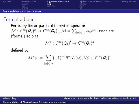
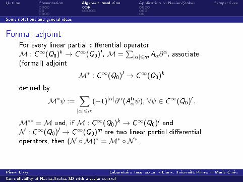
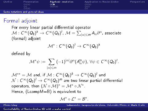
Formal adjointFor every linear partial dierential operator
M : C∞(Q0)k → C∞(Q0)l ,M =∑|α|6m Aα∂
α, associate
(formal) adjoint
M∗ : C∞(Q0)l → C∞(Q0)k
dened by
M∗ψ :=∑|α|6m
(−1)|α|∂α(Atrαψ), ∀ψ ∈ C∞(Q0)l .
M∗∗ =M and, ifM : C∞(Q0)k → C∞(Q0)l andN : C∞(Q0)l → C∞(Q0)m are two linear partial dierential
operators, then (N M)∗ =M∗ N ∗.Hence, (LcompM=B) is equivalent to
M∗ L∗ = B∗.
Pierre Lissy Laboratoire Jacques-Louis Lions, Université Pierre et Marie Curie
Controllability of Navier-Stokes 3D with a scalar control
Outline Presentation Algebraic resolution Application to Navier-Stokes Perspectives
Some notations and general ideas
Formal adjointFor every linear partial dierential operator
M : C∞(Q0)k → C∞(Q0)l ,M =∑|α|6m Aα∂
α, associate
(formal) adjoint
M∗ : C∞(Q0)l → C∞(Q0)k
dened by
M∗ψ :=∑|α|6m
(−1)|α|∂α(Atrαψ), ∀ψ ∈ C∞(Q0)l .
M∗∗ =M and, ifM : C∞(Q0)k → C∞(Q0)l andN : C∞(Q0)l → C∞(Q0)m are two linear partial dierential
operators, then (N M)∗ =M∗ N ∗.
Hence, (LcompM=B) is equivalent to
M∗ L∗ = B∗.
Pierre Lissy Laboratoire Jacques-Louis Lions, Université Pierre et Marie Curie
Controllability of Navier-Stokes 3D with a scalar control
Outline Presentation Algebraic resolution Application to Navier-Stokes Perspectives
Some notations and general ideas
Formal adjointFor every linear partial dierential operator
M : C∞(Q0)k → C∞(Q0)l ,M =∑|α|6m Aα∂
α, associate
(formal) adjoint
M∗ : C∞(Q0)l → C∞(Q0)k
dened by
M∗ψ :=∑|α|6m
(−1)|α|∂α(Atrαψ), ∀ψ ∈ C∞(Q0)l .
M∗∗ =M and, ifM : C∞(Q0)k → C∞(Q0)l andN : C∞(Q0)l → C∞(Q0)m are two linear partial dierential
operators, then (N M)∗ =M∗ N ∗.Hence, (LcompM=B) is equivalent to
M∗ L∗ = B∗.Pierre Lissy Laboratoire Jacques-Louis Lions, Université Pierre et Marie Curie
Controllability of Navier-Stokes 3D with a scalar control
Outline Presentation Algebraic resolution Application to Navier-Stokes Perspectives
A simple example
Presentation of the problem
Introduction
The linearized system
The particular trajectory
Algebraic resolution of dierential systems
Some notations and general ideas
A simple example
Application to the controllability of Navier-Stokes equations
Algebraic solvability and its link with controllability
How to ndMRegular controls of a particular form
PerspectivesPierre Lissy Laboratoire Jacques-Louis Lions, Université Pierre et Marie Curie
Controllability of Navier-Stokes 3D with a scalar control
Outline Presentation Algebraic resolution Application to Navier-Stokes Perspectives
A simple example
A simple case (1)
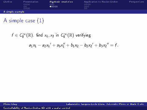
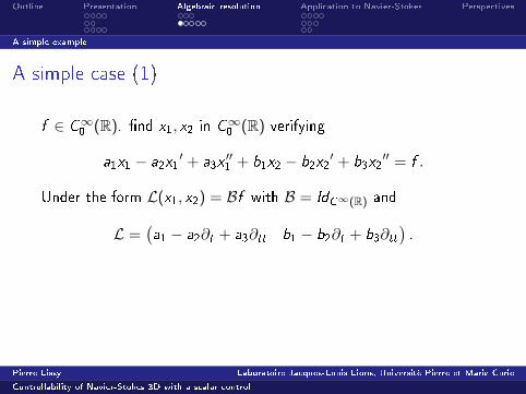
f ∈ C∞0 (R). nd x1, x2 in C∞0 (R) verifying
a1x1 − a2x1′ + a3x
′′1 + b1x2 − b2x2
′ + b3x2′′ = f .
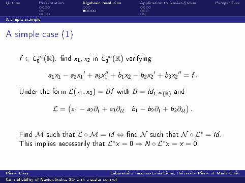
Under the form L(x1, x2) = Bf with B = IdC∞(R) and
L =(a1 − a2∂t + a3∂tt b1 − b2∂t + b3∂tt
).
FindM such that L M = Id ⇔ nd N such that N L∗ = Id .
This implies necessarily that L∗x = 0⇒ N L∗x = x = 0.
Pierre Lissy Laboratoire Jacques-Louis Lions, Université Pierre et Marie Curie
Controllability of Navier-Stokes 3D with a scalar control
Outline Presentation Algebraic resolution Application to Navier-Stokes Perspectives
A simple example
A simple case (1)
f ∈ C∞0 (R). nd x1, x2 in C∞0 (R) verifying
a1x1 − a2x1′ + a3x
′′1 + b1x2 − b2x2
′ + b3x2′′ = f .
Under the form L(x1, x2) = Bf with B = IdC∞(R) and
L =(a1 − a2∂t + a3∂tt b1 − b2∂t + b3∂tt
).
FindM such that L M = Id ⇔ nd N such that N L∗ = Id .
This implies necessarily that L∗x = 0⇒ N L∗x = x = 0.
Pierre Lissy Laboratoire Jacques-Louis Lions, Université Pierre et Marie Curie
Controllability of Navier-Stokes 3D with a scalar control
Outline Presentation Algebraic resolution Application to Navier-Stokes Perspectives
A simple example
A simple case (2)
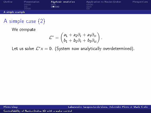
We compute
L∗ =
(a1 + a2∂t + a3∂ttb1 + b2∂t + b3∂tt
).
Let us solve L∗x = 0. (System now analytically overdetermined).
We have to solve a1x + a2x
′ + a3x′′ = 0
b1x + b2x′ + b3x
′′ = 0
We dierentiate. a1x′ + a2x
′′ + a3x′′′ = 0
b1x′ + b2x
′′ + b3x′′′ = 0
Pierre Lissy Laboratoire Jacques-Louis Lions, Université Pierre et Marie Curie
Controllability of Navier-Stokes 3D with a scalar control
Outline Presentation Algebraic resolution Application to Navier-Stokes Perspectives
A simple example
A simple case (2)
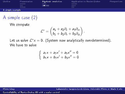
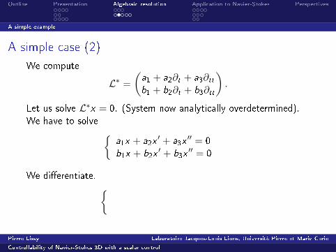
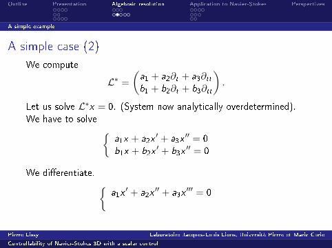
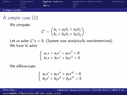
We compute
L∗ =
(a1 + a2∂t + a3∂ttb1 + b2∂t + b3∂tt
).
Let us solve L∗x = 0. (System now analytically overdetermined).
We have to solve a1x + a2x
′ + a3x′′ = 0
b1x + b2x′ + b3x
′′ = 0
We dierentiate.
a1x′ + a2x
′′ + a3x′′′ = 0
b1x′ + b2x
′′ + b3x′′′ = 0
Pierre Lissy Laboratoire Jacques-Louis Lions, Université Pierre et Marie Curie
Controllability of Navier-Stokes 3D with a scalar control
Outline Presentation Algebraic resolution Application to Navier-Stokes Perspectives
A simple example
A simple case (2)
We compute
L∗ =
(a1 + a2∂t + a3∂ttb1 + b2∂t + b3∂tt
).
Let us solve L∗x = 0. (System now analytically overdetermined).
We have to solve a1x + a2x
′ + a3x′′ = 0
b1x + b2x′ + b3x
′′ = 0
We dierentiate. a1x′ + a2x
′′ + a3x′′′ = 0
b1x′ + b2x
′′ + b3x′′′ = 0
Pierre Lissy Laboratoire Jacques-Louis Lions, Université Pierre et Marie Curie
Controllability of Navier-Stokes 3D with a scalar control
Outline Presentation Algebraic resolution Application to Navier-Stokes Perspectives
A simple example
A simple case (2)
We compute
L∗ =
(a1 + a2∂t + a3∂ttb1 + b2∂t + b3∂tt
).
Let us solve L∗x = 0. (System now analytically overdetermined).
We have to solve a1x + a2x
′ + a3x′′ = 0
b1x + b2x′ + b3x
′′ = 0
We dierentiate. a1x′ + a2x
′′ + a3x′′′ = 0
b1x′ + b2x
′′ + b3x′′′ = 0
Pierre Lissy Laboratoire Jacques-Louis Lions, Université Pierre et Marie Curie
Controllability of Navier-Stokes 3D with a scalar control
Outline Presentation Algebraic resolution Application to Navier-Stokes Perspectives
A simple example
A simple case (3)
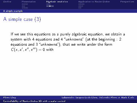
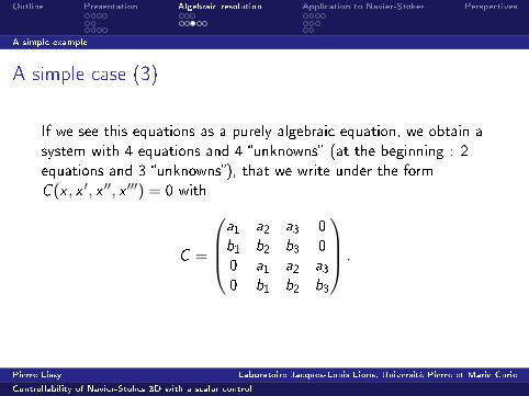
If we see this equations as a purely algebraic equation, we obtain a
system with 4 equations and 4 unknowns (at the beginning : 2
equations and 3 unknowns), that we write under the form
C (x , x ′, x ′′, x ′′′) = 0 with
C =
a1 a2 a3 0
b1 b2 b3 0
0 a1 a2 a30 b1 b2 b3
.
Pierre Lissy Laboratoire Jacques-Louis Lions, Université Pierre et Marie Curie
Controllability of Navier-Stokes 3D with a scalar control
Outline Presentation Algebraic resolution Application to Navier-Stokes Perspectives
A simple example
A simple case (3)
If we see this equations as a purely algebraic equation, we obtain a
system with 4 equations and 4 unknowns (at the beginning : 2
equations and 3 unknowns), that we write under the form
C (x , x ′, x ′′, x ′′′) = 0 with
C =
a1 a2 a3 0
b1 b2 b3 0
0 a1 a2 a30 b1 b2 b3
.
Pierre Lissy Laboratoire Jacques-Louis Lions, Université Pierre et Marie Curie
Controllability of Navier-Stokes 3D with a scalar control
Outline Presentation Algebraic resolution Application to Navier-Stokes Perspectives
A simple example
A simple case (4)
We see that under some conditions on the coecients, necessarily
x ≡ 0. Moreover, one can see C−1 (which acts on x , x ′, x ′′, x ′′′) asa linear partial dierential operator N acting only on x .
Equality C−1C = IdR4 can be written in dierential form
N L∗x = x so thatM = N ∗ gives L M = Id .
Pierre Lissy Laboratoire Jacques-Louis Lions, Université Pierre et Marie Curie
Controllability of Navier-Stokes 3D with a scalar control
Outline Presentation Algebraic resolution Application to Navier-Stokes Perspectives
A simple example
Generalization
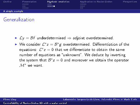
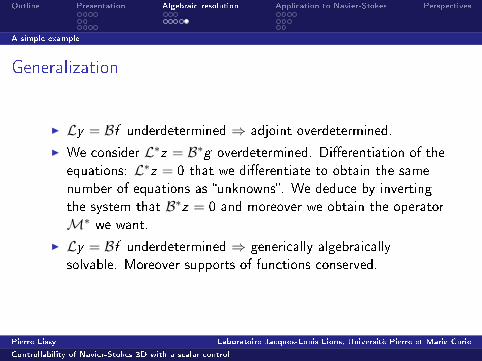
I Ly = Bf underdetermined ⇒ adjoint overdetermined.
I We consider L∗z = B∗g overdetermined. Dierentiation of the
equations: L∗z = 0 that we dierentiate to obtain the same
number of equations as unknowns. We deduce by inverting
the system that B∗z = 0 and moreover we obtain the operator
M∗ we want.
I Ly = Bf underdetermined ⇒ generically algebraically
solvable. Moreover supports of functions conserved.
Pierre Lissy Laboratoire Jacques-Louis Lions, Université Pierre et Marie Curie
Controllability of Navier-Stokes 3D with a scalar control
Outline Presentation Algebraic resolution Application to Navier-Stokes Perspectives
A simple example
Generalization
I Ly = Bf underdetermined ⇒ adjoint overdetermined.
I We consider L∗z = B∗g overdetermined. Dierentiation of the
equations: L∗z = 0 that we dierentiate to obtain the same
number of equations as unknowns. We deduce by inverting
the system that B∗z = 0 and moreover we obtain the operator
M∗ we want.
I Ly = Bf underdetermined ⇒ generically algebraically
solvable. Moreover supports of functions conserved.
Pierre Lissy Laboratoire Jacques-Louis Lions, Université Pierre et Marie Curie
Controllability of Navier-Stokes 3D with a scalar control
Outline Presentation Algebraic resolution Application to Navier-Stokes Perspectives
Algebraic solvability and its link with controllability
Presentation of the problem
Introduction
The linearized system
The particular trajectory
Algebraic resolution of dierential systems
Some notations and general ideas
A simple example
Application to the controllability of Navier-Stokes equations
Algebraic solvability and its link with controllability
How to ndMRegular controls of a particular form
PerspectivesPierre Lissy Laboratoire Jacques-Louis Lions, Université Pierre et Marie Curie
Controllability of Navier-Stokes 3D with a scalar control

Outline Presentation Algebraic resolution Application to Navier-Stokes Perspectives
Algebraic solvability and its link with controllability
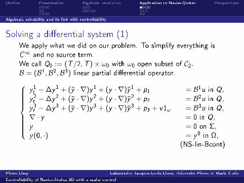
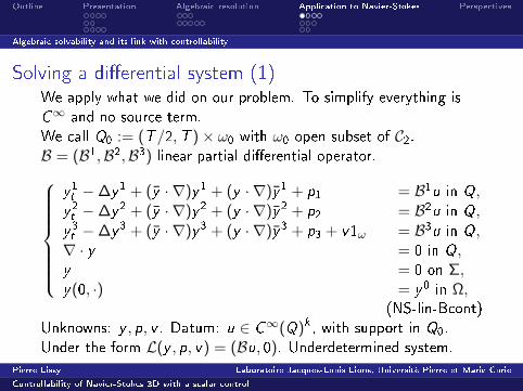
Solving a dierential system (1)We apply what we did on our problem. To simplify everything is
C∞ and no source term.
We call Q0 := (T/2,T )× ω0 with ω0 open subset of C2.B = (B1,B2,B3) linear partial dierential operator.
y1t −∆y1 + (y · ∇)y1 + (y · ∇)y1 + p1 = B1u in Q,
y2t −∆y2 + (y · ∇)y2 + (y · ∇)y2 + p2 = B2u in Q,
y3t −∆y3 + (y · ∇)y3 + (y · ∇)y3 + p3 + v1ω = B3u in Q,∇ · y = 0 in Q,y = 0 on Σ,y(0, ·) = y0 in Ω,
(NS-lin-Bcont)
Unknowns: y , p, v . Datum: u ∈ C∞(Q)k , with support in Q0.
Under the form L(y , p, v) = (Bu, 0). Underdetermined system.
Pierre Lissy Laboratoire Jacques-Louis Lions, Université Pierre et Marie Curie
Controllability of Navier-Stokes 3D with a scalar control
Outline Presentation Algebraic resolution Application to Navier-Stokes Perspectives
Algebraic solvability and its link with controllability
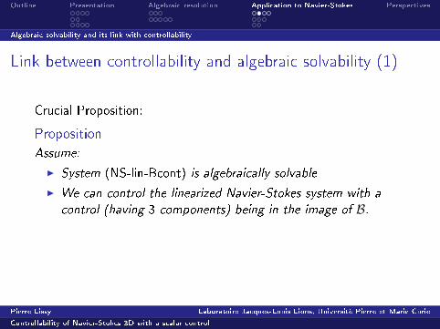
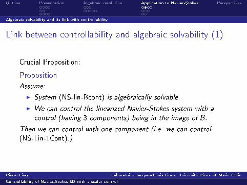
Link between controllability and algebraic solvability (1)
Crucial Proposition:
Proposition
Assume:
I System (NS-lin-Bcont) is algebraically solvable
I We can control the linearized Navier-Stokes system with a
control (having 3 components) being in the image of B.
Then we can control with one component (i.e. we can control
(NS-Lin-1Cont).)
Pierre Lissy Laboratoire Jacques-Louis Lions, Université Pierre et Marie Curie
Controllability of Navier-Stokes 3D with a scalar control
Outline Presentation Algebraic resolution Application to Navier-Stokes Perspectives
Algebraic solvability and its link with controllability
Link between controllability and algebraic solvability (1)
Crucial Proposition:
Proposition
Assume:
I System (NS-lin-Bcont) is algebraically solvable
I We can control the linearized Navier-Stokes system with a
control (having 3 components) being in the image of B.Then we can control with one component (i.e. we can control
(NS-Lin-1Cont).)
Pierre Lissy Laboratoire Jacques-Louis Lions, Université Pierre et Marie Curie
Controllability of Navier-Stokes 3D with a scalar control
Outline Presentation Algebraic resolution Application to Navier-Stokes Perspectives
Algebraic solvability and its link with controllability
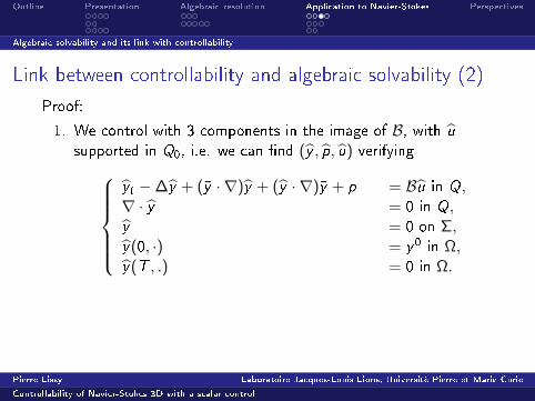
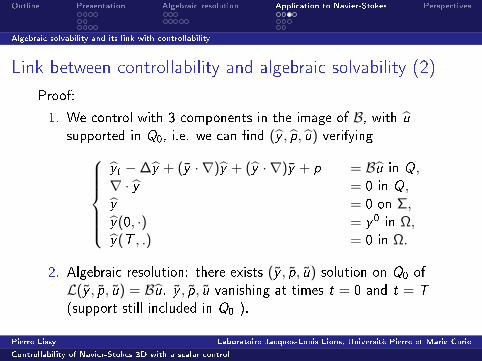
Link between controllability and algebraic solvability (2)
Proof:
1. We control with 3 components in the image of B, with u
supported in Q0, i.e. we can nd (y , p, u) verifyingyt −∆y + (y · ∇)y + (y · ∇)y + p = Bu in Q,∇ · y = 0 in Q,y = 0 on Σ,y(0, ·) = y0 in Ω,y(T , .) = 0 in Ω.
2. Algebraic resolution: there exists (y , p, u) solution on Q0 of
L(y , p, u) = Bu. y , p, u vanishing at times t = 0 and t = T
(support still included in Q0 ).
Pierre Lissy Laboratoire Jacques-Louis Lions, Université Pierre et Marie Curie
Controllability of Navier-Stokes 3D with a scalar control
Outline Presentation Algebraic resolution Application to Navier-Stokes Perspectives
Algebraic solvability and its link with controllability
Link between controllability and algebraic solvability (3)
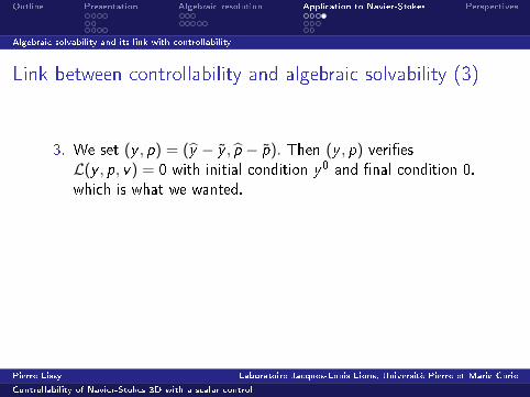
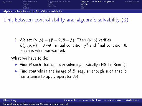
3. We set (y , p) = (y − y , p − p). Then (y , p) veries
L(y , p, v) = 0 with initial condition y0 and nal condition 0,
which is what we wanted.
What we have to do:
I Find B such that one can solve algebraically (NS-lin-Bcont).
I Find controls in the image of B, regular enough such that it
has a sense to apply operatorM.
Pierre Lissy Laboratoire Jacques-Louis Lions, Université Pierre et Marie Curie
Controllability of Navier-Stokes 3D with a scalar control
Outline Presentation Algebraic resolution Application to Navier-Stokes Perspectives
Algebraic solvability and its link with controllability
Link between controllability and algebraic solvability (3)
3. We set (y , p) = (y − y , p − p). Then (y , p) veries
L(y , p, v) = 0 with initial condition y0 and nal condition 0,
which is what we wanted.
What we have to do:
I Find B such that one can solve algebraically (NS-lin-Bcont).
I Find controls in the image of B, regular enough such that it
has a sense to apply operatorM.
Pierre Lissy Laboratoire Jacques-Louis Lions, Université Pierre et Marie Curie
Controllability of Navier-Stokes 3D with a scalar control
Outline Presentation Algebraic resolution Application to Navier-Stokes Perspectives
How to ndM
Presentation of the problem
Introduction
The linearized system
The particular trajectory
Algebraic resolution of dierential systems
Some notations and general ideas
A simple example
Application to the controllability of Navier-Stokes equations
Algebraic solvability and its link with controllability
How to ndMRegular controls of a particular form
PerspectivesPierre Lissy Laboratoire Jacques-Louis Lions, Université Pierre et Marie Curie
Controllability of Navier-Stokes 3D with a scalar control
Outline Presentation Algebraic resolution Application to Navier-Stokes Perspectives
How to ndM
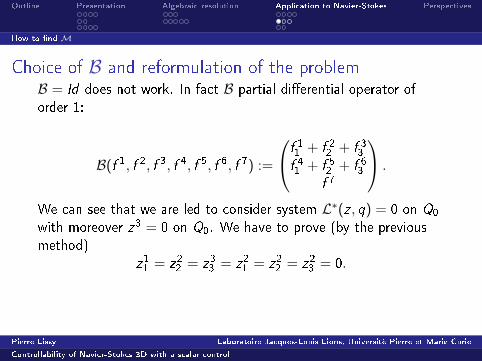
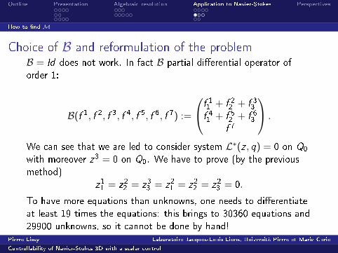
Choice of B and reformulation of the problemB = Id does not work. In fact B partial dierential operator of
order 1:
B(f 1, f 2, f 3, f 4, f 5, f 6, f 7) :=
f 11 + f 22 + f 33f 41 + f 52 + f 63
f 7
.
We can see that we are led to consider system L∗(z , q) = 0 on Q0
with moreover z3 = 0 on Q0. We have to prove (by the previous
method)
z11 = z22 = z33 = z21 = z22 = z23 = 0.
To have more equations than unknowns, one needs to dierentiate
at least 19 times the equations: this brings to 30360 equations and
29900 unknowns, so it cannot be done by hand!
Pierre Lissy Laboratoire Jacques-Louis Lions, Université Pierre et Marie Curie
Controllability of Navier-Stokes 3D with a scalar control
Outline Presentation Algebraic resolution Application to Navier-Stokes Perspectives
How to ndM
Choice of B and reformulation of the problemB = Id does not work. In fact B partial dierential operator of
order 1:
B(f 1, f 2, f 3, f 4, f 5, f 6, f 7) :=
f 11 + f 22 + f 33f 41 + f 52 + f 63
f 7
.
We can see that we are led to consider system L∗(z , q) = 0 on Q0
with moreover z3 = 0 on Q0. We have to prove (by the previous
method)
z11 = z22 = z33 = z21 = z22 = z23 = 0.
To have more equations than unknowns, one needs to dierentiate
at least 19 times the equations: this brings to 30360 equations and
29900 unknowns, so it cannot be done by hand!Pierre Lissy Laboratoire Jacques-Louis Lions, Université Pierre et Marie Curie
Controllability of Navier-Stokes 3D with a scalar control
Outline Presentation Algebraic resolution Application to Navier-Stokes Perspectives
How to ndM
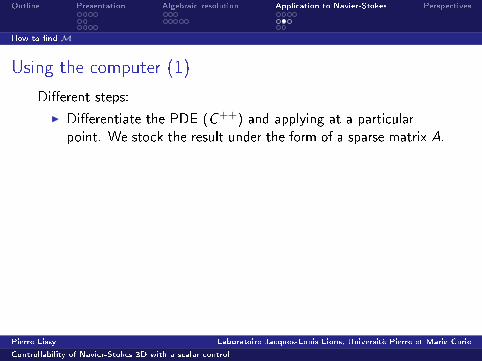
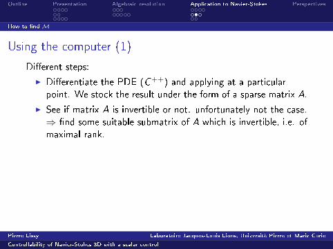
Using the computer (1)
Dierent steps:
I Dierentiate the PDE (C++) and applying at a particular
point. We stock the result under the form of a sparse matrix A.
I See if matrix A is invertible or not. unfortunately not the case.
⇒ nd some suitable submatrix of A which is invertible, i.e. of
maximal rank.
I Rank: a lot of time to compute on a computer. We use
instead the notion of structural rank, which only depend on
the coecients of the matrix that are equal to 0 or not and is
fast to compute. Moreover, there exists an algorithm
(Dulmage-Mendelsohn decomposition) that rearrange the
matrix in a nice way.
Pierre Lissy Laboratoire Jacques-Louis Lions, Université Pierre et Marie Curie
Controllability of Navier-Stokes 3D with a scalar control
Outline Presentation Algebraic resolution Application to Navier-Stokes Perspectives
How to ndM
Using the computer (1)
Dierent steps:
I Dierentiate the PDE (C++) and applying at a particular
point. We stock the result under the form of a sparse matrix A.
I See if matrix A is invertible or not. unfortunately not the case.
⇒ nd some suitable submatrix of A which is invertible, i.e. of
maximal rank.
I Rank: a lot of time to compute on a computer. We use
instead the notion of structural rank, which only depend on
the coecients of the matrix that are equal to 0 or not and is
fast to compute. Moreover, there exists an algorithm
(Dulmage-Mendelsohn decomposition) that rearrange the
matrix in a nice way.
Pierre Lissy Laboratoire Jacques-Louis Lions, Université Pierre et Marie Curie
Controllability of Navier-Stokes 3D with a scalar control
Outline Presentation Algebraic resolution Application to Navier-Stokes Perspectives
How to ndM
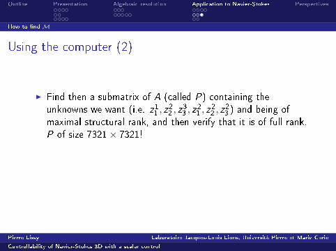
Using the computer (2)
I Find then a submatrix of A (called P) containing the
unknowns we want (i.e. z11 , z22 , z
33 , z
21 , z
22 , z
23 ) and being of
maximal structural rank, and then verify that it is of full rank.
P of size 7321× 7321!
I Use a genericity argument to see that P is invertible
everywhere in Q0 and deduce a dierential operatorM such
that L M = B by inverting P .
Pierre Lissy Laboratoire Jacques-Louis Lions, Université Pierre et Marie Curie
Controllability of Navier-Stokes 3D with a scalar control

Outline Presentation Algebraic resolution Application to Navier-Stokes Perspectives
How to ndM
Using the computer (2)
I Find then a submatrix of A (called P) containing the
unknowns we want (i.e. z11 , z22 , z
33 , z
21 , z
22 , z
23 ) and being of
maximal structural rank, and then verify that it is of full rank.
P of size 7321× 7321!
I Use a genericity argument to see that P is invertible
everywhere in Q0 and deduce a dierential operatorM such
that L M = B by inverting P .
Pierre Lissy Laboratoire Jacques-Louis Lions, Université Pierre et Marie Curie
Controllability of Navier-Stokes 3D with a scalar control
Outline Presentation Algebraic resolution Application to Navier-Stokes Perspectives
Regular controls of a particular form
Presentation of the problem
Introduction
The linearized system
The particular trajectory
Algebraic resolution of dierential systems
Some notations and general ideas
A simple example
Application to the controllability of Navier-Stokes equations
Algebraic solvability and its link with controllability
How to ndMRegular controls of a particular form
PerspectivesPierre Lissy Laboratoire Jacques-Louis Lions, Université Pierre et Marie Curie
Controllability of Navier-Stokes 3D with a scalar control
Outline Presentation Algebraic resolution Application to Navier-Stokes Perspectives
Regular controls of a particular form
Controlling in the image of B (1)
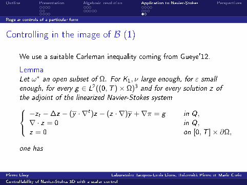
We use a suitable Carleman inequality coming from Gueye'12.
LemmaLet ω∗ an open subset of Ω. For K1, ν large enough, for ε small
enough, for every g ∈ L2((0,T )× Ω)3 and for every solution z of
the adjoint of the linearized Navier-Stokes system−zt −∆z − (y · ∇t)z − (z · ∇)y +∇π = g in Q,∇ · z = 0 in Q,z = 0 on [0,T ]× ∂Ω,
one has
Pierre Lissy Laboratoire Jacques-Louis Lions, Université Pierre et Marie Curie
Controllability of Navier-Stokes 3D with a scalar control

Outline Presentation Algebraic resolution Application to Navier-Stokes Perspectives
Regular controls of a particular form
||e−K1
2r(T−t)5 z ||2L2((T/2,T ),H1(Ω)3) + ||z(T/2, ·)||2L2(Ω)3
6 C
(∫(T/2,T )×Ω
1ω∗e− K1
(T−t)5 |∇ ∧ z |2 +
∫(T/2,T )×Ω
e− K1
(T−t)5 |g |2).
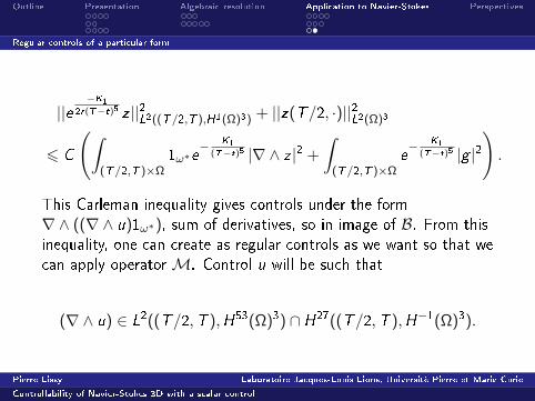
This Carleman inequality gives controls under the form
∇∧ ((∇∧ u)1ω∗), sum of derivatives, so in image of B. From this
inequality, one can create as regular controls as we want so that we
can apply operatorM.
Control u will be such that
(∇∧ u) ∈ L2((T/2,T ),H53(Ω)3) ∩ H27((T/2,T ),H−1(Ω)3).
Pierre Lissy Laboratoire Jacques-Louis Lions, Université Pierre et Marie Curie
Controllability of Navier-Stokes 3D with a scalar control

Outline Presentation Algebraic resolution Application to Navier-Stokes Perspectives
Regular controls of a particular form
||e−K1
2r(T−t)5 z ||2L2((T/2,T ),H1(Ω)3) + ||z(T/2, ·)||2L2(Ω)3
6 C
(∫(T/2,T )×Ω
1ω∗e− K1
(T−t)5 |∇ ∧ z |2 +
∫(T/2,T )×Ω
e− K1
(T−t)5 |g |2).
This Carleman inequality gives controls under the form
∇∧ ((∇∧ u)1ω∗), sum of derivatives, so in image of B. From this
inequality, one can create as regular controls as we want so that we
can apply operatorM. Control u will be such that
(∇∧ u) ∈ L2((T/2,T ),H53(Ω)3) ∩ H27((T/2,T ),H−1(Ω)3).
Pierre Lissy Laboratoire Jacques-Louis Lions, Université Pierre et Marie Curie
Controllability of Navier-Stokes 3D with a scalar control
Outline Presentation Algebraic resolution Application to Navier-Stokes Perspectives
Presentation of the problem
Introduction
The linearized system
The particular trajectory
Algebraic resolution of dierential systems
Some notations and general ideas
A simple example
Application to the controllability of Navier-Stokes equations
Algebraic solvability and its link with controllability
How to ndMRegular controls of a particular form
PerspectivesPierre Lissy Laboratoire Jacques-Louis Lions, Université Pierre et Marie Curie
Controllability of Navier-Stokes 3D with a scalar control
Outline Presentation Algebraic resolution Application to Navier-Stokes Perspectives
Perspectives
I Global controllability around 0,
I Local, global controllability along any trajectory,
I Other coupled systems, for example hyperbolic systems
(non-linear systems of wave equations).
Pierre Lissy Laboratoire Jacques-Louis Lions, Université Pierre et Marie Curie
Controllability of Navier-Stokes 3D with a scalar control
Outline Presentation Algebraic resolution Application to Navier-Stokes Perspectives
Reference
Local null controllability of the three-dimensional Navier-Stokes
system with a distributed control having two vanishing components,
Jean-Michel Coron and Pierre Lissy, submitted.
Thank you for your attention!
Pierre Lissy Laboratoire Jacques-Louis Lions, Université Pierre et Marie Curie
Controllability of Navier-Stokes 3D with a scalar control