Locality Principle Revisited: A Probability-Based Quantitative Approach

Saurabh Gupta, Ping Xiang, Yi Yang, Huiyang Zhou Department of Electrical and Computer Engineering

North Carolina State University Raleigh, USA

sgupta12, pxiang, yyang14, hzhou@ncsu.edu

Abstract—This paper revisits the fundamental concept of the locality of references and proposes to quantify it as a conditional probability: in an address stream, given the condition that an address is accessed, how likely the same address (temporal locality) or an address within its neighborhood (spatial locality) will be accessed in the near future. Based on this definition, spatial locality is a function of two parameters, the neighborhood size and the scope of near future, and can be visualized with a 3D mesh. Temporal locality becomes a special case of spatial locality with the neighborhood size being zero byte. Previous works on locality analysis use stack/reuse distances to compute distance histograms as a measure of temporal locality. For spatial locality, some ad-hoc metrics have been proposed as a quantitative measure. In contrast, our conditional probability-based locality measure has a clear mathematical meaning, offers justification for distance histograms, and provides a theoretically sound and unified way to quantify both temporal and spatial locality.

The proposed locality measure clearly exhibits the inherent application characteristics, from which we can easily derive information such as the sizes of the working data sets and how locality can be exploited. We showcase that our quantified locality visualized in 3D-meshes can be used to evaluate compiler optimizations, to analyze the locality at different levels of memory hierarchy, to optimize the cache architecture to effectively leverage the locality, and to examine the effect of data prefetching mechanisms. A GPU-based parallel algorithm is also presented to accelerate the locality computation for large address traces.

Keywords- locality of references, probability, memory

hierarchy, cache.

I. INTRODUCTION

The locality principle has been widely recognized and leveraged in many disciplines [9]. In computer systems, locality of references is the fundamental principle driving the memory hierarchy design. Specifically, the memory hierarchy relies on two types of locality, temporal and spatial locality. Temporal locality indicates that after an address is referenced, the same datum is likely to be re-referenced in the near future. Spatial locality, on the other hand, indicates that some neighbors of the referenced address are likely to be accessed in the near future. Given the significance of the locality principle, previous works have attempted to quantify the locality to better understand the reference patterns and to guide the compiler and architecture design to enhance/exploit program locality.

Between the two types of locality, the histogram of reuse distances [20] or LRU (least recently used) stack distances [15] computed from an address trace is used as a measure of temporal locality. For spatial locality, however, there is a lack of consensus for such a quantitative measure and several ad-hoc metrics [2][4][11][18] are proposed based on intuitive notions. In this paper, we revisit the concept of locality.

First, we propose to use conditional probabilities as a formal and unified way to quantify both temporal and spatial locality. For any address trace, we define spatial locality as the following conditional probability: for any address, given the condition that it is referenced, how likely an address within its neighborhood will be accessed in the near future. From this definition, we can see that the conditional probability depends on the definition of two parameters, the size of neighborhood and the scope of near future. Therefore, spatial locality is a function of these two parameters and can be visualized with a 3D mesh. Temporal locality is reduced to a special case of spatial locality when the neighborhood size is zero byte.

Second, we examine the relationship between our probability-based temporal locality and the reuse distance histogram, which is used in previous works for quantifying temporal locality. We derive that our proposed temporal locality (using one particular definition of near future) is the cumulative distribution function of the likelihood of reuse in the near future while the reuse histogram is the probability distribution function of the same likelihood, thereby offering theoretical justification for reuse distance histograms. The difference function of our proposed spatial locality over the parameter of the near future window size provides the reuse distance histograms for different neighborhood sizes. In comparison, the difference function of our proposed spatial locality over the parameter of the neighborhood size generates stride histograms for different near future window sizes.

Third, we use the proposed locality to analyze the effect of locality optimizations, sub-blocking/tiling in particular. The quantitative locality presented in 3D meshes visualizes the locality changes for different near future windows and neighborhood sizes, which helps us to evaluate the effectiveness of code optimizations for a wide range of cache configurations.

Fourth, we use the proposed locality to analyze and optimize cache hierarchies. We show that interesting

insights can be revealed from the locality measure of access streams at different levels of memory hierarchy, which can then be used to drive the cache architecture optimization. We also show how the locality correlates to the cache replacement policy. Furthermore, we show that our locality computation can be used to easily evaluate the effect of data prefetchers.

Our proposed locality measure clearly presents the characteristics of a reference stream and helps to reveal interesting insights about the reference patterns. Besides locality analysis, another commonly used way to understand the memory hierarchy performance of an application is through cache simulation. Compared to cache simulation, our proposed measure provides a more complete picture since it provides locality information at various neighborhood sizes and different near future window scopes while one cache simulation only provides one such data point.

The remainder of the paper is organized as follows. Section II defines our probability-based locality, derives the difference functions, and highlights the relationship to reuse distance histograms. Section III focuses on quantitative locality analysis of compiler optimizations for locality enhancement. Section IV discusses locality analysis of cache hierarchies and presents how the visualized locality reveals interesting insights about locality at different levels of cache hierarchy and about data prefetching mechanisms. We also highlight how the locality information helps to drive memory hierarchy optimizations. Section V presents a GPU-based parallel algorithm for our locality computation. Section VI discusses the related work. Finally, Section VII summarizes the key contributions of the paper.

II. QUANTIFYING LOCALITY OF REFERENCE USING

CONDITIONAL PROBABILITES

A. Temporal Locality

Temporal locality captures the characteristics of the same references being reused over time. We propose to quantify it using the following conditional probability: given the condition that an arbitrary address, A, is referenced, the likelihood of the same address to be re-accessed in the near future. Such conditional probability can be expressed as P(Xn = A, ∃n in near future | X0 = A), where X0 is the current reference and Xn is a reference in the near future. Since an address stream usually contains more than one unique address, the temporal locality of an address stream can be expressed as a combined probability, as shown in (1), where M is the number of unique addresses in the stream. , ∃ |

∑ , ∃ | (1) Equation 1 can be further derived using Bayes' theorem,

shown as (2). ∑ , ∃ ∩

(2)

To calculate the joint probabilities, P(Xn = Ai, ∃n in near future ∩ X0 = Ai), we need to formulate a way to define the term ‘near future’. We consider three such definitions and represent temporal locality as TL(N) = P(Xn = A, ∃n < N| X0 = A), where N is the scope of the near future or the future window size. Def. 1 of near future: the next N addresses in the address

stream. Def. 2 of near future: the next N unique addresses in the

address stream. Def. 3 of near future: the next N unique block addresses

in the address stream given a specific cache block size. In other words, we ignore the block offset when we count the next N unique addresses. Based on the definition of the near future, the joint

probability P(X0 = A ∩ Xn = A, ∃n < N) can be computed from an address trace with a moving near future window. In a trace of the length S, for each address (i.e., the event X0 = A), if the same address is also present in the near future window (i.e., the event Xn = A, ∃n < N), we can increment the counter for the joint event (X0 = A ∩ Xn = A, ∃n < N). After scanning the trace, the ratio of this counter over (S – 1) is the probability of P(X0 = A ∩ Xn = A, ∃n < N). The reason for (S – 1) is to account for the fact that there are no more references (or any potential reuse) after the last one in the trace. During the scan through the trace, if def. 1 of near future is used, the moving window has a fixed size while def. 2 and def. 3 require a window of variable sizes. We illustrate the process of calculating temporal locality with an example shown in Figure 1.

(c)

Figure 1. Calculating temporal locality. (a) Reference trace (also showing a moving future window of size 2); (b) Joint probability using Def. 1 of near future; (c) Temporal locality TL(N) using different definitions of near future.

Considering the trace shown in Figure 1, for each address (except the last one), we will examine whether there is a reuse in its near future window. If the near future

Joint probabilities (N = 2) P(X0 = X ∩ Xn = X, ∃n < 2) = 0 P(X0 = Y ∩ Xn = Y, ∃n < 2) = ¼ P(X0 = Z ∩ Xn = Z, ∃n < 2) = 0 So, TL(2) = 0 + ¼ + 0 = ¼

Trace:

(b) (a)

X, Y, Y, X, Z

window size is 2 and we use Def. 1 of near future, we will use a window of size 2 to scan through the trace as shown in Figure 1a. Based on the joint probabilities, the temporal locality, TL(2), is ¼ as shown in Figure 1b. If we follow Def. 2 of near future, the temporal locality, TL(2), is 2/4 since each near future window will contain 2 unique addresses. If we use Def. 3 of near future and assume that X, Y, and Z are in the same block, the temporal locality, TL(2), is 1. The temporal locality with various near future window sizes is shown in Figure 1c for these three definitions of near future.

B. Spatial Locality

Spatial locality captures the characteristics of the addresses within a neighborhood being referenced over time. We propose to quantify it as the following probability: given the condition that an arbitrary address, A, is referenced, the likelihood of an address in its neighborhood to be accessed in the near future. Such conditional probability can be expressed as P(Xn in A’s neighborhood, ∃n < N | X0 = A), where X0 is the current reference and Xn is a reference in the near future. Similar to temporal locality, the spatial locality of an address stream can be computed as the combined probability of all the unique addresses in the trace and it can be expressed as (3), where M is the number of unique addresses in the stream.

, ∃ | ∑ , ∃ | 01

0 ∑ , ∃ ∩ 0 1

(3) To compute the joint probabilities,

, ∃ ∩ , we need to define the meaning of the term ‘neighborhood’ in addition to near future. We consider two definitions for neighborhood and represent spatial locality as SL(N, K), where N is the near future window size and K is a parameter defining the neighborhood size. Def. 1 of neighborhood: an address X is within the

neighborhood of Y if |X – Y| < K, where 2*(K – 1) is the size of the neighborhood. The reason for 2*(K – 1) rather than (K – 1) is to account for the absolute function of (X – Y).

Def. 2 of neighborhood: two addresses X and Y are in the same cache block given the cache block size as K. In other words, X is within the neighborhood of Y if X – (X mod K) = Y – (Y mod K).

Based on the definition of neighborhood, the spatial locality of a reference trace can be computed by moving a near future window through the trace, similar to temporal locality calculation. The difference is that for temporal locality, we require reuses of the same addresses while for spatial locality, the addresses in the window are inspected to see whether there exists a reference Xn , n < N, falling in the neighborhood of X0. If we change the definition of neighborhood size to zero (i.e., K = 1), spatial locality is reduced to temporal locality.

From (3), we can see that spatial locality is a function of two parameters, the neighborhood size, K, and the near future window size, N. As such, we can visualize the spatial locality of an address stream with a 3D mesh or a 2D heat-map for different neighborhood and near future window sizes. Figure 2 shows the spatial locality, using the def. 2 of near future and def. 1 of neighborhood, of the benchmarks SPEC2006 mcf and SPEC2000 bzip2 (see the experimental methodology in Section IV-A). Temporal locality is the curve where the neighborhood size is zero.

Locality visualized in 3D meshes or heat-maps clearly shows the characteristics of reference streams. First, a contour in the 3D mesh/heat-map at a certain locality score (e.g., 0.9) can be used to figure out the sizes of an application’s working data sets. Comparing Figures 2b to 2d, it is evident that bzip2 has a much smaller working data set than mcf. We can also see that the size of the working set varies for different neighborhood sizes. For example, SL(8192, 32) of mcf is close to 0.9, indicating the working set size is slightly bigger than 2*32B*8192 = 512kB when the neighborhood size is 64 (= 2*32) bytes. On the other hand, SL(65536, 16) of mcf is little less than 0.9, showing that the working set is greater than (2*16B*65536) = 2 MB when the neighborhood size is 32(=2*16) bytes.

Second, the quantified locality shows how it can be exploited. From Figure 2a, we can see that for mcf the reuse of the same data at the byte/word granularity (i.e., temporal locality) is limited even with a large near-future window. In contrast, there exists significant spatial locality that can be exploited with a moderate near future window, which also explains why the working set sizes vary significantly for different neighborhood sizes. Bzip2, on the other hand, shows much better temporal and spatial locality, which can be captured effectively with a relatively small neighborhood size. Note that the function SL(N, K) is monotonous along either the N or K direction since our conditional probability definitions are accumulative. In other words, a reuse within a small neighborhood (or close future) is also a reuse for a larger neighborhood (or not-so-close future).

Third, our proposed locality can be used to reveal interesting insights which are typically not present through cache simulations because one cache simulation only provides one data point in this 3D mesh. As one example, the benchmark, hmmer, shows steps in the locality scores (Figure 5a) when the near future size is at 32 and 8192, which implies that there is a good amount of data locality that we cannot leverage until we can explore the reuse distance of 8192. Such observations from the 3D mesh enable us to understand why and whether a particular cache configuration performs much better than the other ones.

Between heat maps and 3D meshes, locality presented in heat-maps better reveals the working set information. On the other hand, 3D-meshes are more useful in showing how the locality changes along either the neighborhood size or the near future window size, which indicates how the locality can be exploited.

Different definitions of ‘near future’ lead to different near future window sizes as illustrated in Figure 1. Such differences, however, turn out to have little impact when we compute locality for most SPEC CPU benchmarks. Between the two definitions of neighborhood, although def. 2 models the cache behavior more accurately, it fails to capture spatial locality across the block boundary. For example, for a perfect stride pattern, 1, 2, 3, 4, 5, …, the spatial locality using neighborhood def. 1 will be 1 for any neighborhood size and any future window size greater than 0. If we use def. 2 of neighborhood, the spatial locality will be dependent upon the neighborhood (or cache block) size. If the neighborhood/block size is 2 bytes, the spatial locality is 0.5

for any future window size. If the neighborhood/block size is B bytes, the spatial locality becomes (B – 1)/B for any future window size greater than or equal to B. In Figure 3, we show the spatial locality for the benchmark sphinx with neighborhood def. 1 (Figure 3a) and def. 2 (Figure 3b). From the figure, we can observe the similar behavior, i.e., increasing locality values for larger neighborhood sizes in Figure 3b. In contrast, Figure 3a shows a stepwise increase in locality values. Based on these observations, we choose to use def. 2 of near future and def. 1 of neighborhood for locality analysis. Whenever the objective is to estimate the cache performance, def. 3 of near future and def. 2 of neighborhood can be used instead.

(a) (b)

Figure 3. Spatial locality of the benchmark sphinx for neighborhood definitions. (a) definition 1 (b) definition 2.

(c) bzip2 (SPEC2000) 3D-mesh

(a) mcf (SPEC2006) 3D-mesh

(d) bzip2 (SPEC2000) heat-map

Figure 2. The spatial locality plots of the benchmarks, mcf (SPEC2006) and bzip2 (SPEC2000). Temporal locality is a special case of spatial locality with nighborhood size as 0.

(b) mcf (SPEC2006) heat-map

C. The Relationship between Spatial and Temporal Locality

Based on our probability-based definitions of spatial and temporal locality, temporal locality can be viewed as a special case of spatial locality. Beyond this observation, there also exist some intriguing subtleties between the two types of locality. In particular, we can change the neighborhood definition in spatial locality so that the exact same addresses are excluded from the neighborhood. In other words, the neighborhood definition becomes 0 < |X – Y| < K. In this case, an interesting question is: for any address trace, is the sum of its spatial locality and its temporal locality always less than or equal to 1?

An apparent answer is yes since the reuses from the same addresses are excluded from the neighborhood definition. This is also our initial understanding until our locality computation results show otherwise. After a detailed analysis, it is found that the events for temporal and spatial locality are not always disjoint and therefore the sum can be larger than 1. To elaborate, we use def. 1 of near future and def. 1 of neighborhood with the modification that same addresses being excluded. Other definitions of the two terms can be applied similarly. Following (1) and (3), temporal and spatial locality can be expressed as the following two conditional probabilities: P(Xn = A, ∃ | X0 = A) and P(0 < |Xn – A| < K, ∃ | X0 = A), respectively. Both probabilities can be computed using the sum of the joint probabilities ∑ (Xn = Ai, ∃ ∩ X0 = Ai) and ∑ (0 < |Xn – Ai| < K, ∃ ∩ X0 = Ai). Since each Ai is unique, the events X0 = Ai are disjoint for different Ai. So, we can focus on one such address, e.g., A1. We can use the Venn diagram to capture the relationship among the events: X0 = A1, X1 = A1 + ∆, and X2 = A1, as shown in Figure 4. From Figure 4, we can see that (X0 = A1 ∩ X2 = A1) and (X0 = A1 ∩ X 1 = A1 + ∆) are not disjoint. An intuitive explanation is that for an address sequence such as A1, A1+1, A1, the third reference (A1) contributes to both temporal locality of the first reference and spatial locality of the second reference. Therefore, the events for temporal and spatial locality are not disjoint although the references to same addresses are excluded from the neighborhood definition.

D. Difference Functions of Locality Measures and the Relationship to Reuse Distance Histograms

Next, we derive the relationship of our probability-based temporal locality to reuse distance histograms, which are commonly used in previous works to quantify temporal locality. In sequential execution, reuse distance is the number of distinct data elements accessed between two consecutive references to the same element. The criterion to determine the ‘same’ element is based on the cache-block granularity, i.e., the block offsets are omitted when determining reuses. The reuse distance provides a capacity requirement for fully associative LRU caches to fully exploit the reuses. The histogram of reuse distances is used as the quantitative locality signature of a trace since it captures all the reuses at different distances. Based on our probability-based measure, temporal locality TL(N) represents the probability P(Xn = A, ∃n < N| X0 = A). As this probability is a discrete function of N, we can take a difference function of temporal locality ∆TL(N) = TL(N) – TL(N – 1) = P(XN-1 = A | X0 = A). This function represents the frequency of reuses at the exact reuse distance of (N – 1). If we use def. 3 of the term near future, the difference function becomes: ∆TL(N) = P(XN-1 = block_addr(A) | X0 = A) where block_addr(A) = A – (A mod block_size) and it is essentially the same as the reuse distance histogram. Therefore, we conclude that the reuse histogram is the probability distribution function of the event (XN-1 = A | X0 = A) and our proposed temporal locality is the accumulative distribution function of the same event.

As spatial locality, SL(N, K), is a function of two parameters, the near future window size N and the neighborhood size K, we can compute the difference function of SL(N, K) over either parameter and both difference functions reveal interesting insights of the access patterns.

Similar to temporal locality, the difference function of spatial locality over N, SL(N, K) – SL(N – 1, K) = P( (XN-1 – XN-1 mod K) = (A – A mod K) | X0 = A), shows the reuse distance histograms with different block sizes, K, if we follow def. 2 of neighborhood.

The difference function over the neighborhood size parameter, K, can be derived as follows: SL(N, K) – SL(N, K – 1) = P(|Xn – A| = K – 1, ∃n < N | X0 = A). This probability function represents that in an address trace how often a stride pattern with a stride of (K – 1) happens in a near future window of size N. For different N and K, this function essentially provides a histogram of different strides for any given near future window size. In the context of processor caches, this difference function helps to reason about the relationship among the cache sizes, which determine the maximum reuse distance or near future window size, the block sizes, which determine the neighborhood sizes, and the performance potential of stride prefetchers.

X0 = A1

X2 = A1

X1 = A1+∆

Figure 4. The Venn diagram showing the relationship among events X0 = A1, X1 = A1 + ∆, and X2 = A1.

In Figure 5, we present the spatial locality information (Figure 5a) of the benchmark, hmmer, and its two difference functions (Figures 5b and 5c). From the Figure 5b, we can see how the reuse distance histograms vary for different block sizes. For small block sizes, many reuses can only be captured with long reuse distances. For large block sizes, the reuse distance becomes much smaller. This clearly indicates that one reuse histogram is not sufficient to understand the reuse patterns. Based on Figure 5c, we can see that for small near future windows, there are limited stride accesses. When the near future window size increases (larger than 32), the stride access pattern (stride of 8 bytes) is discovered. It implies that although the application has strong spatial locality in the forms of stride access patterns, in order to exploit such spatial locality, the cache size and set associativity need to be large enough to prevent a cache block from being replaced before it is re-accessed. In addition, the single dominant stride suggests that a stride prefetcher can be an effective way to improve the performance for this benchmark.

E. Sub-trace Locality

The locality defined in (1) and (3) includes reuses of all

the addresses in a reference stream. Therefore, it can be viewed as ‘whole-trace’ locality. We can add constraints to focus on certain reuses of interest, e.g., the locality of one memory access instruction or accesses to one data structure, within the address trace. We refer such locality to as sub-trace locality as not all the reuses in the trace will be considered. Note that sub-trace locality is usually not the same as the locality computed from the filtered trace, e.g., the addresses generated by one instruction, because the filtered trace will miss the constructive cross-references from other instructions. Instead, sub-trace locality is computed from the ‘whole’ trace. Mathematically, sub-trace spatial locality (STSL) can be defined and derived as the sum of the joint probabilities as shown in (4). Sub-trace temporal locality (STTL) can be derived similarly.

, ∃ , ∈ 0 , 0∈

∑ , ∃ ∩∩ ∈ ∩ ∈ (4)

From (4), it can be seen that compared to whole trace locality, sub-trace locality is modeled with the additional joint events, ∈ ∩ ∈ , in the joint probability computation. The definition of SetX and SetY determines the event of interest. For example, to compute the locality of one particular memory access instruction, we can define SetX as the addresses generated by the instruction of interest and define SetY as the whole sample space Ω or addresses generated by all instructions, meaning that for all the addresses (i.e., ( ∩ ∈

), we need to check whether there is a spatial reuse in the near future by the instruction of interest

, ∃ ∩ ∈.If we change SetY to SetX, the equation calculates

the locality of the address trace generated by the instruction of interest (i.e., the filtered trace).

We can make a slight change to (4) so that it can be (a)

(b) (c)

Figure 5. Locality and the difference functions for the benchmark hmmer. (a) Spatial Locality (b) Difference function over the near future window size N, which is the same as reuse distance histograms (c) Difference function over neighborhood size K, which shows a histogram of stride access patterns.

computed more efficiently. Instead of looking for reuses in a near future window, we can use a near past window, as shown in (5). This way, we can compute the locality of an instruction of interest as follows, for each address generated by the instruction (i.e., the event: ∩ ∈ , we search in a near past window for spatial reuse (i.e., the event:

, ∃ , 0 ∩ ∈ .)

∑ , ∃ , 0 ∩ ∩ ∈ ∩ ∈ (5)

Another use of sub-trace locality is to analyze the effectiveness of data prefetching. For example, consider the following address trace containing both demand requests (underlined addresses) and prefetch requests: A, A+32, A+64, A+96, A+128, A+64, A+128, A+160, A+192. In this case, we can define SetX = demand requests and SetY = combined demand and prefetch requests. Then, sub-trace locality provides the information that for a demand request, how likely there are prefetch requests (or demand requests) for the same address in a near past window. The locality of either the demand request trace or the combined demand and prefetch request trace does not provide such information.

III. LOCALITY ANALYSIS FOR CODE OPTMIZATIONS

In this section, we use sub-blocking / tiling to show how our proposed measure can be used to analyze and visualize the locality improvement of code optimizations.

To analyze the locality improvement of the sub-blocking/tiling optimization, we choose to use the matrix multiplication kernel C = A x B and we use the pin tool [14] to instrument the binaries to generate the memory access traces for our locality computation. We used def. 1 of near future and def. 1 of neighborhood in our locality computation. Figure 6 shows the locality information collected for different versions of the kernel, including un-tiled, tiled with the tile size of 32x32, and the tiled with the size 64x16. The matrix size is 256x256.

In the un-tiled matrix multiplication kernel, the matrix A is accessed along each row in the sequence. Therefore, it exhibits spatial locality when the neighborhood size ≥ 4 bytes, which is the size of each data element. Since the accesses to the matrices A and B are interleaved and B is accessed column-wise (i.e., no spatial locality at this

neighborhood size), such spatial locality shows up when the near future window size ≥ 2 and the locality score is 0.5. The kernel keeps using the same row from A until it is done with all the columns of matrix B. Consequently, after every 256 accesses along the row from A, the same elements are re-accessed. Again, due to the interleaved accesses of A and B as well as the accesses to the production matrix C, the reused distance actually is more than 512 (256 from matrix A + 256 from matrix B + 1 from matrix C) and hence the temporal locality appears at near future window size of 1024 in Figure 6a. Accesses to the matrix B do not repeat until 256x256x2 = 128k accesses, which is why temporal locality for the maximum near future value in Figure 6a is still around 50%. Since the matrix B is accessed column-wise, with the near future window size of 1024 and neighborhood size of 4, accesses to the matrix B start to enjoy spatial locality (i.e., B[i][j] and B[i][j+1] show in the same window) and the locality becomes very close to 1 as shown in Figure 6a.

With the loop tiling optimization, both matrices A and B are divided into tiles/sub-blocks. This reduces the reuse distance of the data elements as we can see from Figures 6b and 6c. For a tile size of 32x32, the inner loops perform matrix multiplication of two 32x32 matrices. As a result, the sub-blocks of A get reused when the near future window is larger than 64 and the sub-blocks of B get reused when the near future window is 2048 (= 32x32x2). The sub-blocks of matrix A are accessed row-wise and show 0.5 spatial locality when the neighborhood size is 4 bytes and near future window is smaller than 64. The sub-blocks of the matrix B show spatial locality when the near future window is larger than 64, which makes B[ii][jj] and B[ii][jj+1] show up in the same window. The 3D locality mesh shown in Figure 6b visualizes these changes in both temporal and spatial locality and confirms the observations. When the tile size is 64x16, the locality information, shown in Figure 6c, is the same as matrix multiplication of a 64x16 matrix with a 16x64 matrix.

Based on the locality information shown in Figure 6, we can easily see how much and where the locality improvement has been achieved with code optimizations. Furthermore, if we use def. 3 of near future and def. 2 of

(a) (b) (c)

Figure 6. Locality for different matrix multiplication kernels (a) Untiled (b) 32x32 tile (c) 64x16 tile.

neighborhood, we can also use our locality function to infer how much locality a specific cache can capture. For example, an 8kB cache with a 16-byte block size will be able to explore the future window up to 512 (8kB/16 bytes) and neighborhood range of 16 bytes. Therefore, SL(512, 16) will show the hit rate of this cache if it is fully associative. Mathematical models proposed in [6][13][17] can also be used to estimate miss rates for set-associative caches from the fully associative ones.

IV. LOCALITY ANALYSIS FOR MEMORY HIERARCHY

OPTMIZATIONS

Our proposed locality measure provides quantitative locality information at different neighborhood sizes and near future scopes. In this section, we show that it reveals interesting insights to drive memory hierarchy optimizations.

A. Experimental Methodology

In this section, we use an in-house execution driven simulator developed based on SimpleScalar [5] for our study, except stated otherwise in Section IV-E. In our simulator, we model a 4-way issue superscalar processor. The memory hierarchy contains a 32kB 4-way set-associative L1 data cache with the block size of 64 bytes (3 cycle hit latency), a 32kB 2-way set associative L1 instruction cache, and a unified 8-way set associative 1MB L2 cache with the block size of 64 bytes (30 cycle hit latency). The main memory latency is set as 200 cycles (224 cycles) to get a 64-byte (128-byte) L2 block. The memory bus runs at 800MHz while the processor core runs at 2GHz.

We include all the SPEC 2000 and SPEC 2006 benchmarks that we were able to compile and run for SimpleScalar ISA (PISA), 16 from SPEC 2000 and 8 from

SPEC 2006. Benchmarks mcf and bzip2 from SPEC2006 are abbreviated as mcf-2006 and bzip2-2006. For each benchmark, we use a representative 100M Simpoint [12] for our trace collection and simulations. In our locality computation, we use the def. 2 of near future and def. 1 of neighborhood.

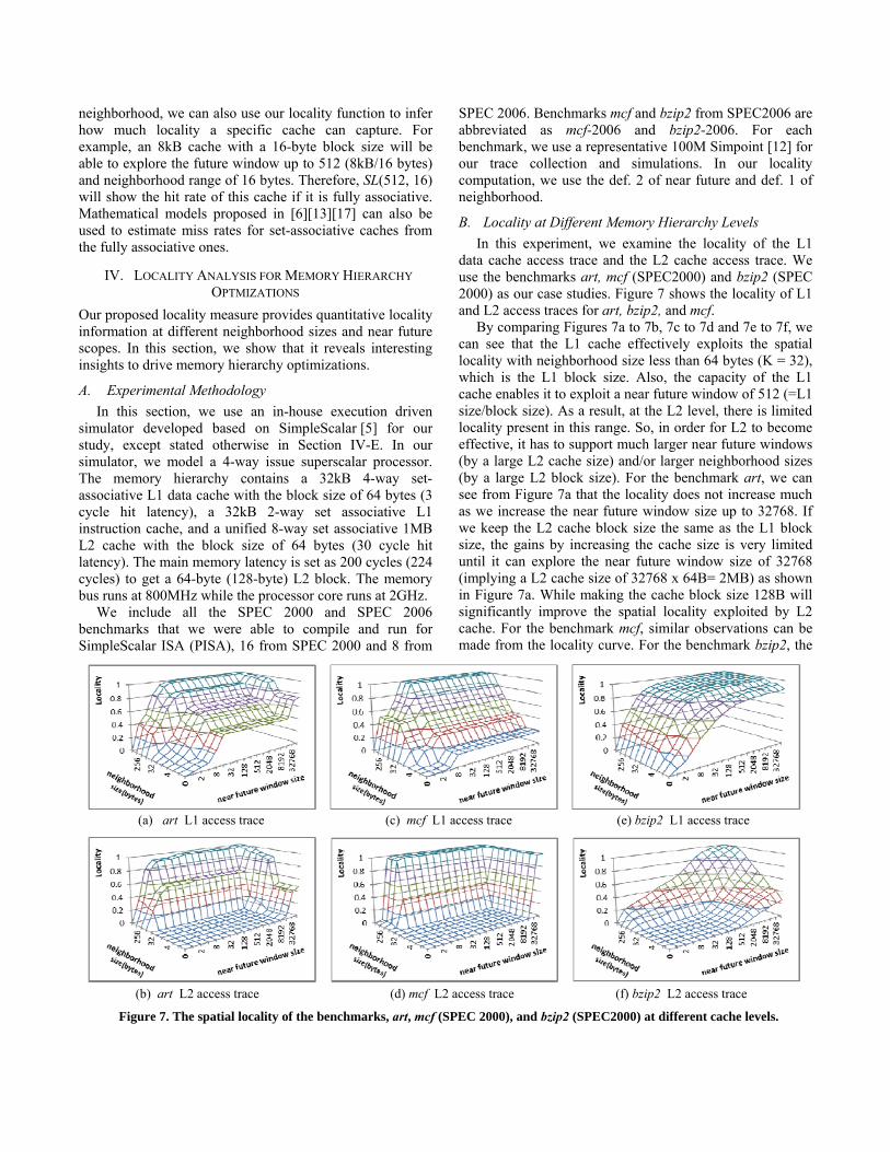
B. Locality at Different Memory Hierarchy Levels In this experiment, we examine the locality of the L1

data cache access trace and the L2 cache access trace. We use the benchmarks art, mcf (SPEC2000) and bzip2 (SPEC 2000) as our case studies. Figure 7 shows the locality of L1 and L2 access traces for art, bzip2, and mcf.

By comparing Figures 7a to 7b, 7c to 7d and 7e to 7f, we can see that the L1 cache effectively exploits the spatial locality with neighborhood size less than 64 bytes (K = 32), which is the L1 block size. Also, the capacity of the L1 cache enables it to exploit a near future window of 512 (=L1 size/block size). As a result, at the L2 level, there is limited locality present in this range. So, in order for L2 to become effective, it has to support much larger near future windows (by a large L2 cache size) and/or larger neighborhood sizes (by a large L2 block size). For the benchmark art, we can see from Figure 7a that the locality does not increase much as we increase the near future window size up to 32768. If we keep the L2 cache block size the same as the L1 block size, the gains by increasing the cache size is very limited until it can explore the near future window size of 32768 (implying a L2 cache size of 32768 x 64B= 2MB) as shown in Figure 7a. While making the cache block size 128B will significantly improve the spatial locality exploited by L2 cache. For the benchmark mcf, similar observations can be made from the locality curve. For the benchmark bzip2, the

(a) art L1 access trace (c) mcf L1 access trace (e) bzip2 L1 access trace

(b) art L2 access trace (d) mcf L2 access trace (f) bzip2 L2 access trace

Figure 7. The spatial locality of the benchmarks, art, mcf (SPEC 2000), and bzip2 (SPEC2000) at different cache levels.

spatial locality of the L2 accesses is lower than the other two benchmarks in Figure 7.

C. Understanding the Replacement Policy

It has been well understood that some applications work well with the least recently used (LRU) replacement policy while others do not. We examine this question using our probability-based locality. We first focus on L1 cache access streams. Figure 7e (or Figure 2b) shows that with block size larger than 4 bytes, bzip2 features a high amount of locality within small near future windows. For larger windows, the locality improvement is pretty much saturated. This implies that the L1 access stream of bzip2 is LRU friendly as most of the data or their neighbors will be used in a ‘short/small’ near future window. In comparison, if we look at the locality of the L1 accesses for mcf (SPEC2006), shown in Figure 2a, the locality is very gradual when the block size is less than 4 bytes and there is no “knee” behavior along the X axis (the near future window size) as has been observed in bzip2. This shows that in mcf, many data reuses require long reuse distance, which is not LRU friendly as they are likely to become least recently used before they are re-accessed. Interestingly, if we look at the other dimension of the 3D mesh for mcf, we can see that it becomes more LRU friendly for as neighborhood size goes up (i.e., when the cache block sizes ≥ 4 bytes).

Next, we examine the L2 access streams. As discussed in Section IV-B, the L1 cache effectively exploits the locality in small near future windows and the L2 cache has to explore a larger near future window to capture the remaining locality. From Figure 7f, we can see that for bzip2, with the neighborhood size being 64 bytes (K = 32), once the window becomes reasonably large (e.g., 16384, corresponding to a 1MB =16384*64 B cache), there exists significant locality. Therefore, it is still LRU friendly. In contrast, the locality is not present for small near future windows for benchmarks art or mcf (SPEC 2000) (Figure 7b and 7d). This suggests that for art or mcf, there are many reuses at the L2 level requiring very long reuse distances. For an L2 cache with limited capacity (less than 2MB), the LRU replacement policy does not work well since the cache is not able to sustain such large reuse distances and exhibits thrashing behavior. For such access patterns, thrash resistant replacement policies such as DIP [16] can be a better choice. The locality plot also reveals that it gets more reuse (or becomes more LRU friendly) if the cache block size is larger than 64 bytes.

D. Memory Hierarchy Optimizations

1) Optimizing Last-Level Caches (LLC):

In order to improve the performance of the last-level cache, the L2 cache in our simulator, we examine the locality information of the L2 access stream. The L2 access locality of art and mcf is shown in Figures 7b and 7d. In Figure 8, we report the locality information of L2 access streams of the SPEC benchmarks, sphinx, wupwise, ammp,

milc, mesa, gcc, equake, vortex and swim. Two important observations can be made from the locality results. First, a common theme of all the locality information is that there exists strong spatial locality when the neighborhood size is larger than 32 bytes, corresponding to a cache block size of 64 bytes given our neighborhood definition 1. The behavior is expected as the L1 cache block size is 64 bytes. However, in many current commercial processors, the same cache block size (e.g., 64 bytes in Intel Core i7) is used for different level of caches to simplify the cache coherence management. From the locality information shown in Figure 8, we can see that many benchmarks require much larger neighborhood sizes to take advantage the spatial locality. Among these benchmarks, wupwise, milc, mesa, equake, vortex and gcc would need the neighborhood size of 64 bytes (i.e., 128-byte cache block) while sphinx, mcf and art exhibit additional spatial locality for increasing neighborhood sizes. The benchmark, ammp, requires a neighborhood size of 2048 bytes due to its streaming access pattern with a stride of more than 1024 bytes.

Second, for all these benchmarks, the spatial locality can be exploited within a small near future window (or reuse distance) when a large block is used. This indicates that a small cache with relatively large block sizes can be more effective than a large cache with small block sizes. For example, for benchmark gcc, SL(4,64) = 0.97 (corresponding to a 4x128 = 512 byte cache with the 128-byte block size) is higher than SL(8192,32) = 0.008 (corresponding to a 8192 * 64 = 512KB cache with a 64-byte block size) and is very close to SL(16384, 32) = 0.99 (corresponding to a 16384*64 = 1MB cache with a 64-byte block size). Since most of the locality can be captured within a small near future window, it also means that the LRU replacement policy will work well for caches with large blocks as discussed in Section IV-C, thereby eliminating the need for more advanced replacement policies. Furthermore, the limited near future window indicates that the required set associativity is small as well.

Different approaches can be used to achieve the effect of large-block caches. The first method is to directly increase the cache block size. The advantage is that it can reduce the required cache size as discussed above. The downside is that it may not work for all applications because different applications prefer different block sizes. The second method is to emulate the big block size by augmenting the cache with next-n-line / previous-n-line prefetching. The way to determine the value ‘n’ in next/previous-n-line prefetching is based on our locality measure. With the current block size of 64 bytes, if there is high spatial locality at block size of 128 bytes, e.g., gcc, next/previous line prefetch is used (i.e., n=1). If the spatial locality shows up at a much larger block size, e.g., 2kB for ammp, n is set as 2kB/64B = 32. In other words, our locality measure can be used a profiling tool to control the next/previous-n-line prefetching. The advantage of this approach is that it can emulate different cache block sizes without changing the cache configurations (i.e., cache

size, set associativity, and block size). The third way is to use a stream buffer to detect stride patterns and prefetch data blocks into caches.

Next, we evaluate the effectiveness using our locality measure with a case study on the benchmark wupwise. Here we use the locality measure of the L2 demand miss stream as it shows the locality that the L2 cache fails to exploit. In Figures 9a, 9b, and 9c, we show the L2 miss locality measure for wupwise when the L2 cache uses a 64-byte block size, a 128-byte block size, and a stream- buffer. The next/previous line prefetch has very similar results to the cache with the 128-byte block size. From Figure 9a, we can see that the L2 cache with a 64-byte block size fails to exploit the spatial locality at large neighborhood sizes. In contrast, Figure 9b shows that the 128-byte block cache with the same size exploits the spatial locality effectively. The stream prefetcher does not work as well for wupwise as the stride access patterns are not common in this benchmark. Our timing simulation also confirms the similar trend in performance improvement for wupwise: an execution-time reduction of 5% using the stream buffer while the 128-byte

block size and next line prefetching achieve the execution-time reduction of 11% to 14%, respectively.

Figure 10 shows IPC speedup results for large block sizes, next/previous-n-line prefetching, and stream buffer prefetcher. Among the benchmarks, equake, gap, hmmer, mcf(SPEC2000), mcf (SPEC2006), milc, parser, perl, and wupwise favor large block sizes (or previous/next-n-line prefetching). On average, 4.7% (6.6%) IPC improvement is achieved on average across all the benchmarks using large block sizes (previous/next-n-line prefetching). Benchmark swim experiences a slowdown when bigger block size or next/previous-n-line prefetching is used. The results can be explained with the locality of its L2 access trace (Figure 8i). From the figure, we can see that the difference in locality score, when the block size is changed from 64 bytes to 128 bytes, is very small for swim. Therefore, the increased latency to get a larger data block results in a slowdown. Benchmarks ammp, art, gap and lbm have stride beyond 64 bytes, therefore 128 byte block size is not much helpful for these benchmarks. We determine the more suitable ‘n’ value to be used in next/previous nth-line prefetcher from the

Figure 8. The spatial locality of L2 access traces for various benchmarks.

(a) sphinx (b) wupwise (c) ammp

(d) milc (e) mesa (f) gcc

(g) equake (h) vortex (i) swim

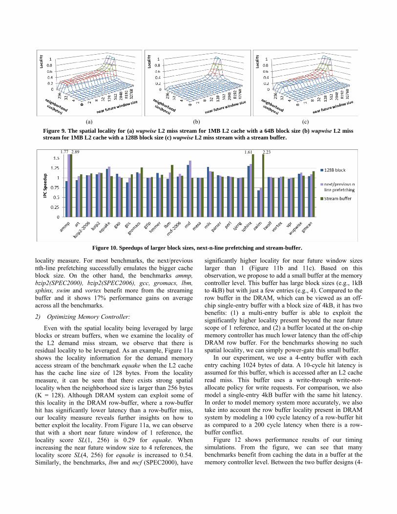
locality measure. For most benchmarks, the next/previous nth-line prefetching successfully emulates the bigger cache block size. On the other hand, the benchmarks ammp, bzip2(SPEC2000), bzip2(SPEC2006), gcc, gromacs, lbm, sphinx, swim and vortex benefit more from the streaming buffer and it shows 17% performance gains on average across all the benchmarks.

2) Optimizing Memory Controller:

Even with the spatial locality being leveraged by large blocks or stream buffers, when we examine the locality of the L2 demand miss stream, we observe that there is residual locality to be leveraged. As an example, Figure 11a shows the locality information for the demand memory access stream of the benchmark equake when the L2 cache has the cache line size of 128 bytes. From the locality measure, it can be seen that there exists strong spatial locality when the neighborhood size is larger than 256 bytes (K = 128). Although DRAM system can exploit some of this locality in the DRAM row-buffer, where a row-buffer hit has significantly lower latency than a row-buffer miss, our locality measure reveals further insights on how to better exploit the locality. From Figure 11a, we can observe that with a short near future window of 1 reference, the locality score SL(1, 256) is 0.29 for equake. When increasing the near future window size to 4 references, the locality score SL(4, 256) for equake is increased to 0.54. Similarly, the benchmarks, lbm and mcf (SPEC2000), have

significantly higher locality for near future window sizes larger than 1 (Figure 11b and 11c). Based on this observation, we propose to add a small buffer at the memory controller level. This buffer has large block sizes (e.g., 1kB to 4kB) but with just a few entries (e.g., 4). Compared to the row buffer in the DRAM, which can be viewed as an off-chip single-entry buffer with a block size of 4kB, it has two benefits: (1) a multi-entry buffer is able to exploit the significantly higher locality present beyond the near future scope of 1 reference, and (2) a buffer located at the on-chip memory controller has much lower latency than the off-chip DRAM row buffer. For the benchmarks showing no such spatial locality, we can simply power-gate this small buffer.

In our experiment, we use a 4-entry buffer with each entry caching 1024 bytes of data. A 10-cycle hit latency is assumed for this buffer, which is accessed after an L2 cache read miss. This buffer uses a write-through write-not-allocate policy for write requests. For comparison, we also model a single-entry 4kB buffer with the same hit latency. In order to model memory system more accurately, we also take into account the row buffer locality present in DRAM system by modeling a 100 cycle latency of a row-buffer hit as compared to a 200 cycle latency when there is a row-buffer conflict.

Figure 12 shows performance results of our timing simulations. From the figure, we can see that many benchmarks benefit from caching the data in a buffer at the memory controller level. Between the two buffer designs (4-

Figure 9. The spatial locality for (a) wupwise L2 miss stream for 1MB L2 cache with a 64B block size (b) wupwise L2 miss stream for 1MB L2 cache with a 128B block size (c) wupwise L2 miss stream with a stream buffer.

(a) (b) (c)

Figure 10. Speedups of larger block sizes, next-n-line prefetching and stream-buffer.

2.231.77 2.89

1.61

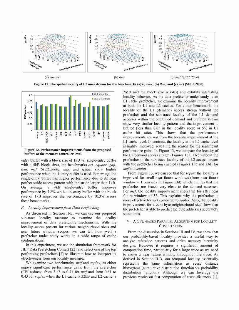
entry buffer with a block size of 1kB vs. single-entry buffer with a 4kB block size), the benchmarks art, equake, gap, lbm, mcf (SPEC2000), milc and sphinx show higher performance when the 4-entry buffer is used. For ammp, the single-entry buffer has higher performance due to its near perfect stride access pattern with the stride larger than 1kB. On average, a 4kB single-entry buffer improves performance by 7.8% while a 4-entry buffer with the block size of 1kB improves the performance by 10.3% across these benchmarks.

E. Locality Improvement from Data Prefetching

As discussed in Section II-E, we can use our proposed sub-trace locality measure to examine the locality improvement of data prefetching mechanisms. With the locality scores present for various neighborhood sizes and near future window scopes, we can tell how well a prefetcher under study works in a wide range of cache configurations.

In this experiment, we use the simulation framework for JILP Data Prefetching Contest [22] and select one of the top performing prefetchers [7] to illustrate how to interpret its effectiveness from our locality measure.

We examine two benchmarks, mcf and soplex, as either enjoys significant performance gains from the prefetcher (CPI reduced from 3.17 to 0.71 for mcf and from 0.61 to 0.43 for soplex when the L1 cache is 32kB and L2 cache is

2MB and the block size is 64B) and exhibits interesting locality behavior. As the data prefetcher under study is an L1 cache prefetcher, we examine the locality improvement at both the L1 and L2 caches. For either benchmark, the locality of the L1 (demand) access stream without the prefetcher and the sub-trace locality of the L1 demand accesses within the combined demand and prefetch stream show very similar locality pattern and the improvement is limited (less than 0.05 in the locality score or 5% in L1 cache hit rate). This shows that the performance improvements are not from the locality improvement at the L1 cache level. In contrast, the locality at the L2 cache level is highly improved, revealing the reason for the significant performance gains. In Figure 13, we compare the locality of the L2 demand access stream (Figures 13a, 13c) without the prefetcher to the sub-trace locality of the L2 access stream with the prefetcher being enabled (Figures 13b and 13d) for mcf and soplex.

From Figure 13, we can see that for soplex the locality is improved for small near future windows (from near future window = 1 onwards in Figure 13d) which implies that the prefetches are issued very close to the demand accesses. For mcf, the locality improvement shows up for after near future window of 32. This explains why the prefetcher is more effective for mcf compared to soplex. Also, the locality improvements for a zero byte neighborhood size show that the prefetcher is able to predict the byte addresses accurately sometimes.

V. A GPU-BASED PARALLEL ALGORITHM FOR LOCALITY

COMPUTATION

From the discussion in Sections III and IV, we show that our probability-based locality provides a useful way to analyze reference patterns and drive memory hierarchy designs. However it requires a significant amount of computation time, particularly for a large trace as we need to move a near future window throughout the trace. As derived in Section II-D, our temporal locality essentially represents the same information as reuse distance histograms (cumulative distribution function vs. probability distribution function). Although we can leverage the previous works on fast computation of reuse distances [1],

Figure 12. Performance improvements from the proposed buffers at the memory controller level.

Figure 11. The spatial locality of L2 miss stream for the benchmarks (a) equake; (b) lbm; and (c) mcf (SPEC2000).

(a) equake (b) lbm (c) mcf (SPEC2000)

we aim to reduce the computation time by an order of magnitude to make it practical for compiler or runtime profile analysis. Based on the inherent data-level parallelism of our locality computation, we resort to parallel computation on graphics processing units (GPUs).

Our parallel algorithm for locality computation of an address trace A[0 : S-1] is outlined as follows.

1. Each thread will be responsible to the locality information of A[thread id]. More specifically, it calculates the joint probability

, ∃ ∩ for a specific neighborhood size K. It does so by comparing A[thread id] with A[thread id + 1], A[thread id + 2], A[thread id + 3], etc., until it exceeds the maximal near future window size or finds an address meeting the requirement of neighborhood. We keep W counters in each thread for W different near future window sizes. When an address in its neighborhood is found, the distance to A[thread id] is determined. If the distance is smaller than a near future window size, the corresponding counter is incremented.

2. After we obtain the locality information of each address, we need to combine them to generate the locality information of the trace. Since we have W counters in each thread, we will perform W reductions across all threads to accumulate them. After reduction, those accumulated counters are divided by S to generate the data points of the locality function, i.e., SL(1, K), SL(2, K), SL(4, K), …, SL(2W, K).

3. Repeat steps 1 and 2 for a different neighborhood size K.

We implement this algorithm using CUDA [21]. In our implementation, both steps 1 and 2 are optimized by utilizing GPU’s on-chip shared memory. We run our GPU algorithm on a NVIDIA GTX480 GPU and compare with our CPU implementation on an Intel Core i7 920 processor. We compute locality with the near future window size ranging from 1 to 216 addresses (exponential scale) and we vary the neighborhood size from 0 to 512 bytes (exponential scale). For address traces with the length of 1 million to 16 million addresses, our GPU implementation takes less than 4 seconds and achieves 30X to 33X speedups over our CPU implementation.

(a)

(c)

(b)

Figure 13. The locality improvement of mcf and soplex at the L2 cache level (a) the locality of the L2 demand accesses of mcf without the prefetcher, (b) the sub-trace locality of the L2 demand trace of mcf with the prefetcher, (c) the locality of the L2 demand accesses of soplex without the prefetcher, (d) the sub-trace locality of the L2 demand trace of soplex with the prefetcher.

(d)

VI. RELATED WORK

Given its importance, the principle of locality has been extensively studied. However, most previous works on quantifying locality, spatial locality in particular, are based on intuitive notions or heuristics and there is a lack for formal quantitative definition of locality.

For temporal locality, reuse distances or LRU stack distances [15] are used to determine how far in the future a temporal reuse is going to happen. The histogram of reuse distances is used as a signature to quantify the temporal locality of a trace [20]. StatCache [3] provides an efficient way to estimate reuse distance histograms through sampling. Section II-D derives the relationship between our probability-based measures and reuse histograms and provides a theoretical justification for reuse histograms. Based on this relationship, previous works on reuse distances such as component-based locality analysis [8][19] can also be adapted to our proposed measure. In [10], mass-count disparity is used to show that most reuses are from accessing a small number of addresses.

For spatial locality, Bunt et al. [4] assume that the references can be fit to a Brad-Zipf distribution and the parameters of such a distribution are used to generate a spatial locality score. Weinberg et al. [18] propose to compute a histogram of different strides within a window of previously accessed addresses and then combine the histogram with strides into a single score for spatial locality. Berg et al. [2] and Gu et al. [11] propose to quantify the spatial locality effect using the changes in the miss rates or the reuse histograms when the block size is increased or doubled.

Using a 3D surface to visualize locality is proposed in [23] and it is recognized that the temporal locality is a special case of spatial locality. The locality measure in [23] is based on an averaged probability that the next access is within a stride of the current location within a near future window, which is fundamentally different from our proposed conditional probability.

Compared to previous attempts on quantifying temporal or spatial locality, the advantages of our proposed approach include: (1) it provides a numeric measure with a clear mathematical meaning (i.e., conditional probability); (2) it offers a unified quantification for both temporal and spatial locality; and (3) it does not only present a single locality score for a specific cache configuration but also shows the trend of how locality vary when we change the near future window and neighborhood size so that we can better understand the nature of the program locality.

VII. CONCLUSIONS

The locality principle describes the phenomenon that after a reference to a datum, the same datum or its neighbors are likely to be referenced in near future. This paper addresses the question ‘how likely’. The key contribution of the paper includes (a) a formal definition of locality as a

conditional probability and derivation of how it can be computed using joint probabilities, which can in turn be computed from address traces, (b) the derivation of difference functions of the locality function and the justification for reuse histograms as a quantitative measure of temporal locality, (c) the formal definition of sub-trace locality to focus on certain reuses of interest, and (d) various locality analysis using our proposed measure, revealing the following insights (1) how locality can be exploited at different levels of memory hierarchy and how the locality curves drive various memory optimizations; (2) the information of the working set: instead of the common way of using the knee of the miss rate curve over cache sizes, the working set is represented as a contour in a 3D surface showing the same conditional probability can be exploited using different neighborhood sizes and near future scopes; (3) an evaluation of memory optimizations such as data prefetcher over a wide range of cache configurations.

ACKNOWLEDGMENT

We would like to thank the anonymous reviewers for their insightful comments to improve our paper. This research is supported by an NSF grant CNS-0905223, an NSF CAREER award CCF-0968667 and a research fund from Intel Corporation.

REFERENCES [1] G. Almasi et al., “Calculating stack distances efficiently”, In

MSP, 2002. [2] E. Berg and E. Hagersten, “Fast Data-Locality Profiling of

Native Execution”, In SIGMETRICS’05, 2005. [3] E. Berg and E. Hagersten, “Statcache: A probabilistic

approach to efficient and accurate data locality analysis.” In IEEE ISPASS, 2004

[4] R. Bunt and J. Murphy, “The Measurement of Locality and the Behavior of Programs”, The Computer Journal, 1984.

[5] D. Burger and T. M. Austin, “The Simplescalar Tool Set Version 2.0”, Technical Report, Computer Science Department, University of Wisconsin-Madison, 1997

[6] C. Caşcaval and D. Padua, “Estimating Cache Misses and Locality Using Stack Distances”, In ICS, 2003.

[7] M. Dimitrov et al., “Combining Local and Global History for High Performance Data Prefetching”. In the JILP Data Prefetching Championship, 2009.

[8] C. Ding and Y. Zhong, “Predicting whole-program locality with reuse distance analysis”, In PLDI, 2003.

[9] P. Denning, “The Locality Principle”, Communications of ACM, 2005.

[10] Y. Etsion and D. G. Feitelson, “L1 cache filtering through random selection of memory references”. In PACT-16, 2007.

[11] X. Gu, et al., “A Component Model of Spatial Locality”, In ISMM’09, 2009.

[12] G. Hamerly, E. Perelman, J. Lau, and B. Calder. “SimPoint 3.0: Faster and More Flexible Program Analysis.” In MoBS, 2005.

[13] M. Hill and A. J. Smith, “Evaluating Associativity in CPU caches”, In IEEE TC, 1989.

[14] C. Luk, et al., “Pin: building customized program analysis tools with dynamic instrumentation”, In PLDI, 2005.

[15] R. Mattson et al., “Evaluation Techniques for Storage Hierarchies”, IBM System Journal, 1970.

[16] M. Qureshi, et al., “Adaptive Insertion Policies for High Performance Caching”, In ISCA-34, 2007.

[17] J. Smith, “A Comparative Study of Set Associative Memory Mapping Algorithms and Their Use for Cache and Main Memory”, IEEE TSE, 1978.

[18] J. Weinberg, et al., “Quantifying Locality In the Memory Access Patterns of HPC Applications”, In SC’05, 2005.

[19] Y. Zhong et al., “Miss Rate Prediction across Program Inputs and Cache Configurations”, IEEE TC, 2007.

[20] Y. Zhong, et al., “Program Locality Analysis Using Reuse Distance”, ACM TOPLAS, 2009.

[21] NVIDIA CUDA Programming Guide, Version 2.2, 2009. [22] The 1st JILP Data Prefetching Championship (DPC-1)

(http://www.jilp.org/dpc), 2009. [23] K. Grimsrud and J. Archibald, “Locality As a Visualization

Tool”, IEEE Trans. on Computers, Vol. 45, No. 11, 1996.