Localization in geometry and physics

Vasily PestunInstitut des Hautes Études Scientifiques

06 February 2019, Foundations of Geometric Structures of Information

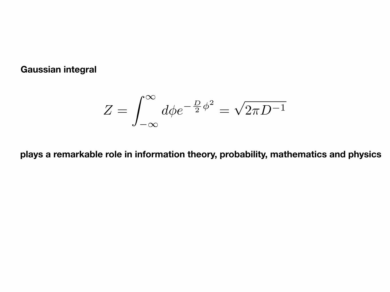
Gaussian integral

plays a remarkable role in information theory, probability, mathematics and physics

Z =

Z 1

�1d�e�

D2 �2

=p2⇡D�1

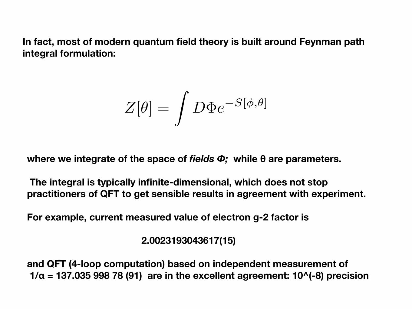
In fact, most of modern quantum field theory is built around Feynman path integral formulation:

Z[✓] =

ZD�e�S[�,✓]

where we integrate of the space of fields Ф; while θ are parameters.

The integral is typically infinite-dimensional, which does not stop practitioners of QFT to get sensible results in agreement with experiment.

For example, current measured value of electron g-2 factor is 2.0023193043617(15)

and QFT (4-loop computation) based on independent measurement of 1/α = 137.035 998 78 (91) are in the excellent agreement: 10^(-8) precision

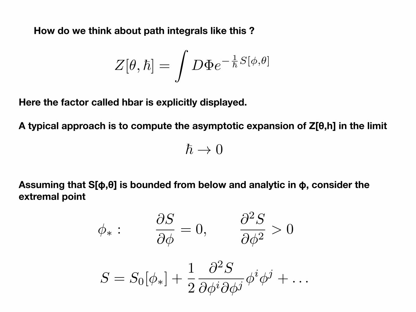
How do we think about path integrals like this ?

Z[✓, ~] =Z

D�e�1~S[�,✓]

Here the factor called hbar is explicitly displayed.

A typical approach is to compute the asymptotic expansion of Z[θ,h] in the limit

~ ! 0

Assuming that S[φ,θ] is bounded from below and analytic in φ, consider the extremal point

�⇤ :@S

@�= 0,

@2S

@�2> 0

S = S0[�⇤] +1

2

@2S

@�i@�j�i�j + . . .

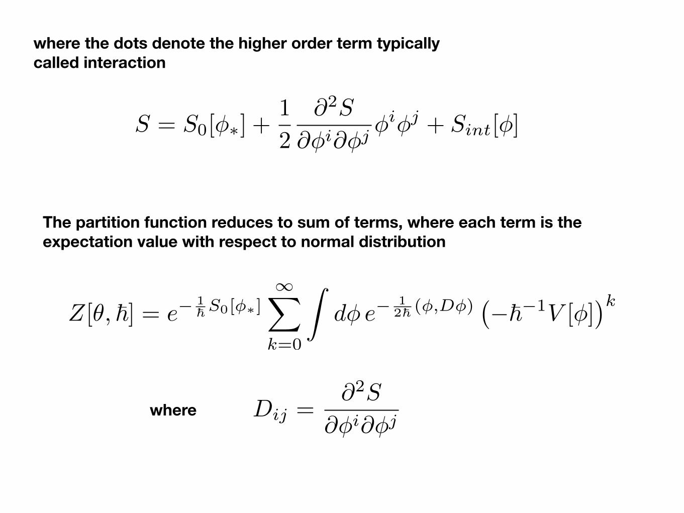
where the dots denote the higher order term typically called interaction

S = S0[�⇤] +1

2

@2S

@�i@�j�i�j + Sint[�]

The partition function reduces to sum of terms, where each term is the expectation value with respect to normal distribution

Z[✓, ~] = e�1~S0[�⇤]

1X

k=0

Zd� e�

12~ (�,D�)

��~�1V [�]

�k

Dij =@2S

@�i@�jwhere

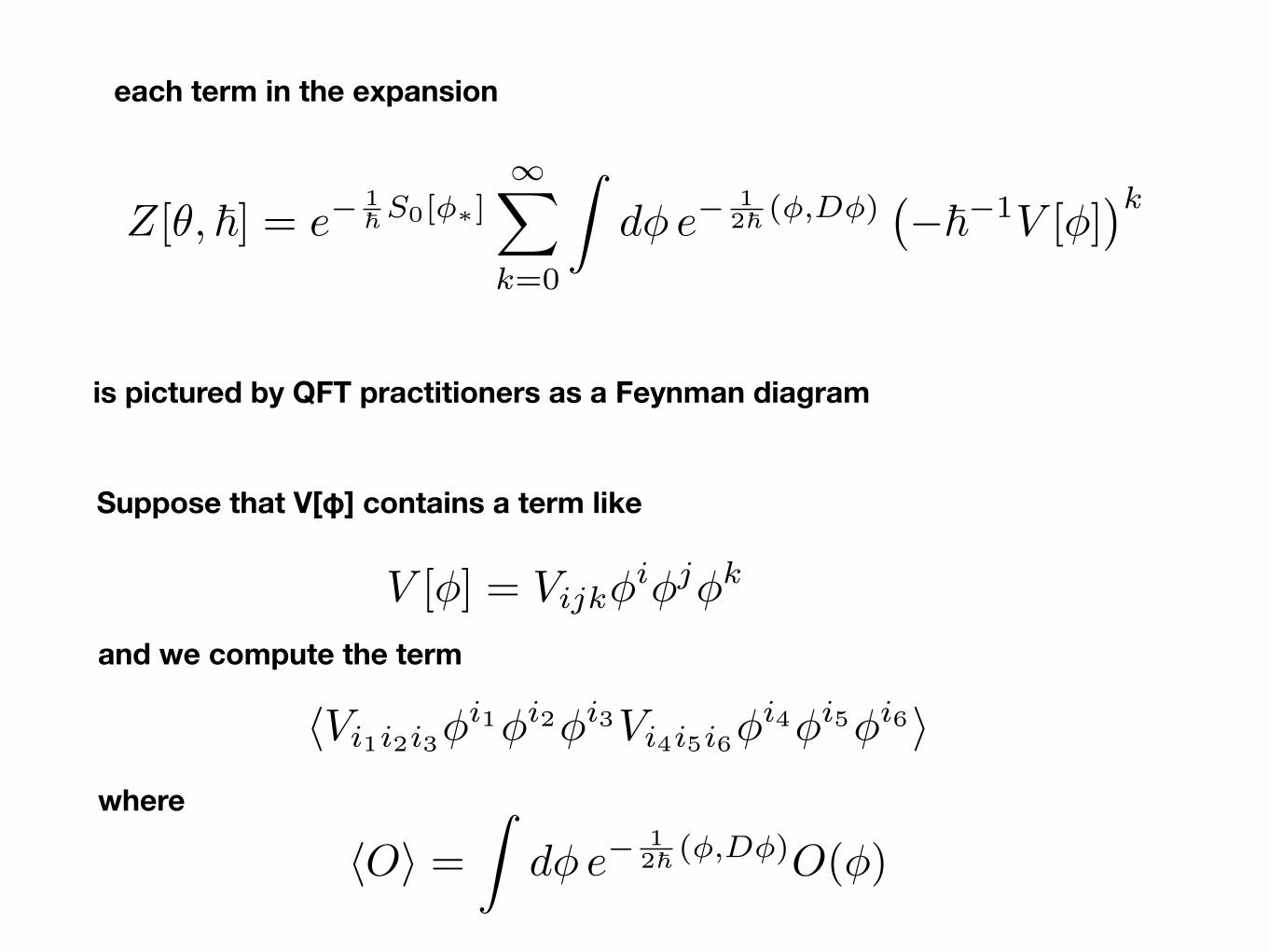
Z[✓, ~] = e�1~S0[�⇤]

1X

k=0

Zd� e�

12~ (�,D�)

��~�1V [�]

�k

each term in the expansion

is pictured by QFT practitioners as a Feynman diagram

Suppose that V[φ] contains a term like

V [�] = Vijk�i�j�k

and we compute the term

hVi1i2i3�i1�i2�i3Vi4i5i6�

i4�i5�i6i

hOi =Z

d� e� 1

2~ (�,D�)O(�)

where

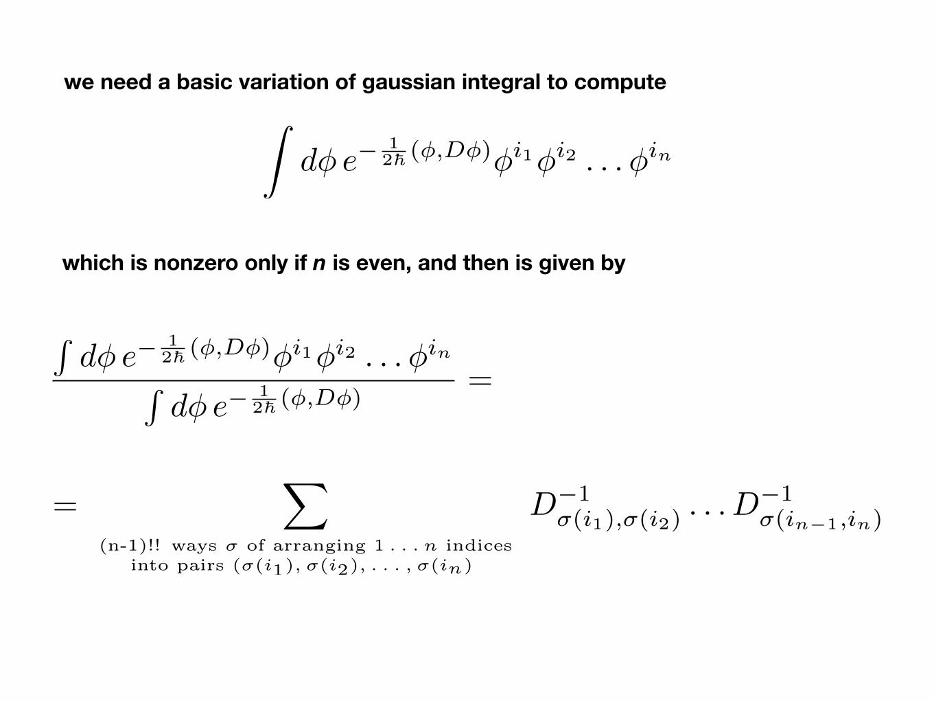
we need a basic variation of gaussian integral to computeZ

d� e�12~ (�,D�)�i1�i2 . . .�in

which is nonzero only if n is even, and then is given by

Rd� e�

12~ (�,D�)�i1�i2 . . .�in

Rd� e�

12~ (�,D�)

=

=X

(n-1)!! ways � of arranging 1 . . . n indicesinto pairs (�(i1), �(i2), . . . , �(in)

D�1�(i1),�(i2)

. . . D�1�(in�1,in)

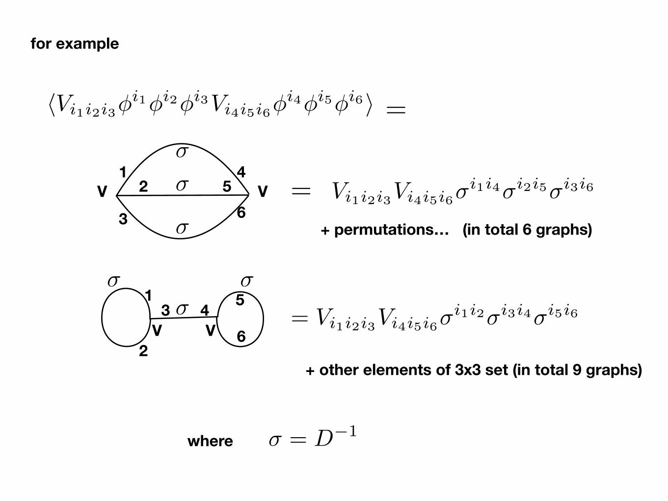
for example

hVi1i2i3�i1�i2�i3Vi4i5i6�

i4�i5�i6i

Vi1i2i3Vi4i5i6�i1i4�i2i5�i3i6

=

V V

V V

�

�

�

� ��

=

= Vi1i2i3Vi4i5i6�i1i2�i3i4�i5i6

+ permutations… (in total 6 graphs)

+ other elements of 3x3 set (in total 9 graphs)

12

3

45

6

1

2

3 4 5

6

� = D�1where

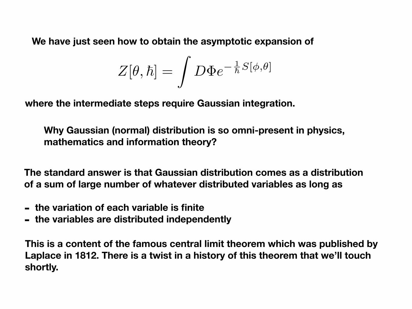
We have just seen how to obtain the asymptotic expansion of

Z[✓, ~] =Z

D�e�1~S[�,✓]

where the intermediate steps require Gaussian integration.

Why Gaussian (normal) distribution is so omni-present in physics, mathematics and information theory?

The standard answer is that Gaussian distribution comes as a distribution of a sum of large number of whatever distributed variables as long as

- the variation of each variable is finite - the variables are distributed independently

This is a content of the famous central limit theorem which was published by Laplace in 1812. There is a twist in a history of this theorem that we’ll touch shortly.

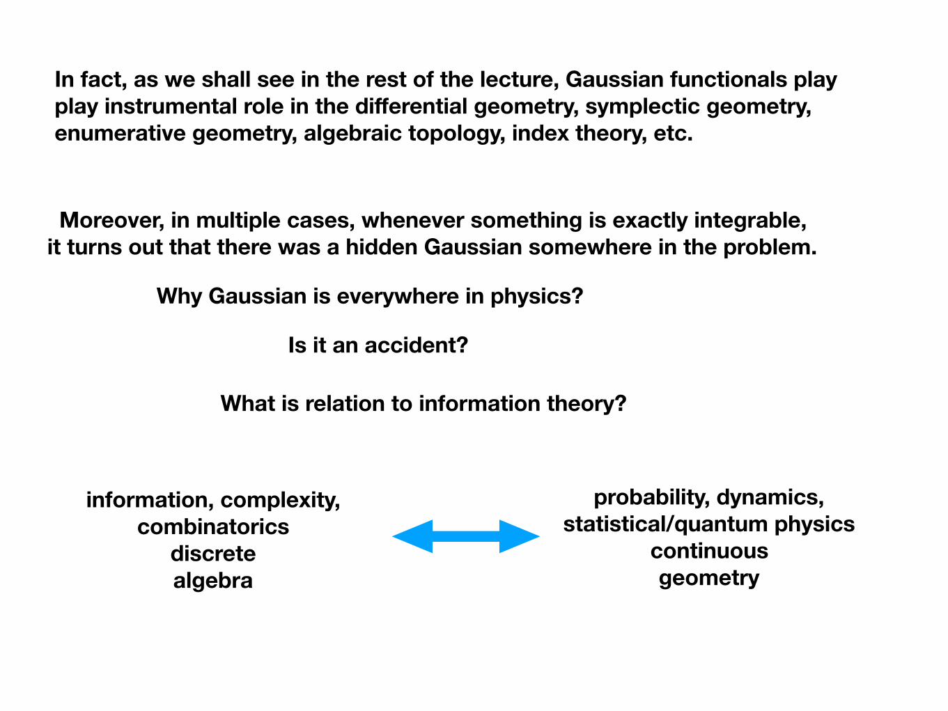
In fact, as we shall see in the rest of the lecture, Gaussian functionals play play instrumental role in the differential geometry, symplectic geometry, enumerative geometry, algebraic topology, index theory, etc.

Why Gaussian is everywhere in physics?

Moreover, in multiple cases, whenever something is exactly integrable, it turns out that there was a hidden Gaussian somewhere in the problem.

Is it an accident?

What is relation to information theory?

information, complexity, combinatorics

discrete algebra

probability, dynamics, statistical/quantum physics

continuous geometry

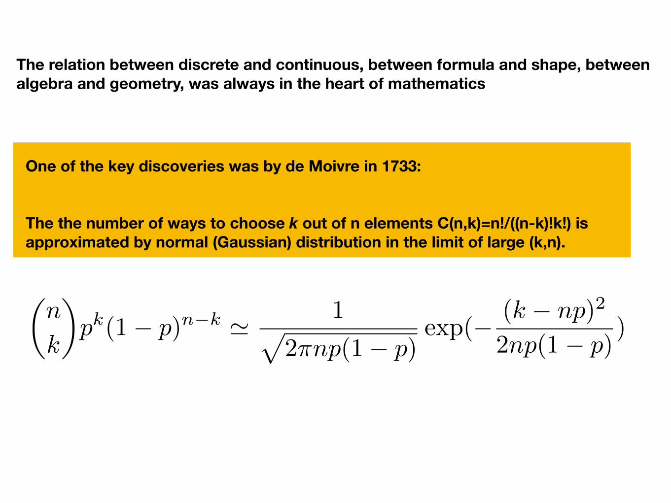
The relation between discrete and continuous, between formula and shape, between algebra and geometry, was always in the heart of mathematics

One of the key discoveries was by de Moivre in 1733:

The the number of ways to choose k out of n elements C(n,k)=n!/((n-k)!k!) is approximated by normal (Gaussian) distribution in the limit of large (k,n).

✓n

k

◆pk(1� p)n�k ' 1p

2⇡np(1� p)exp(� (k � np)2

2np(1� p))

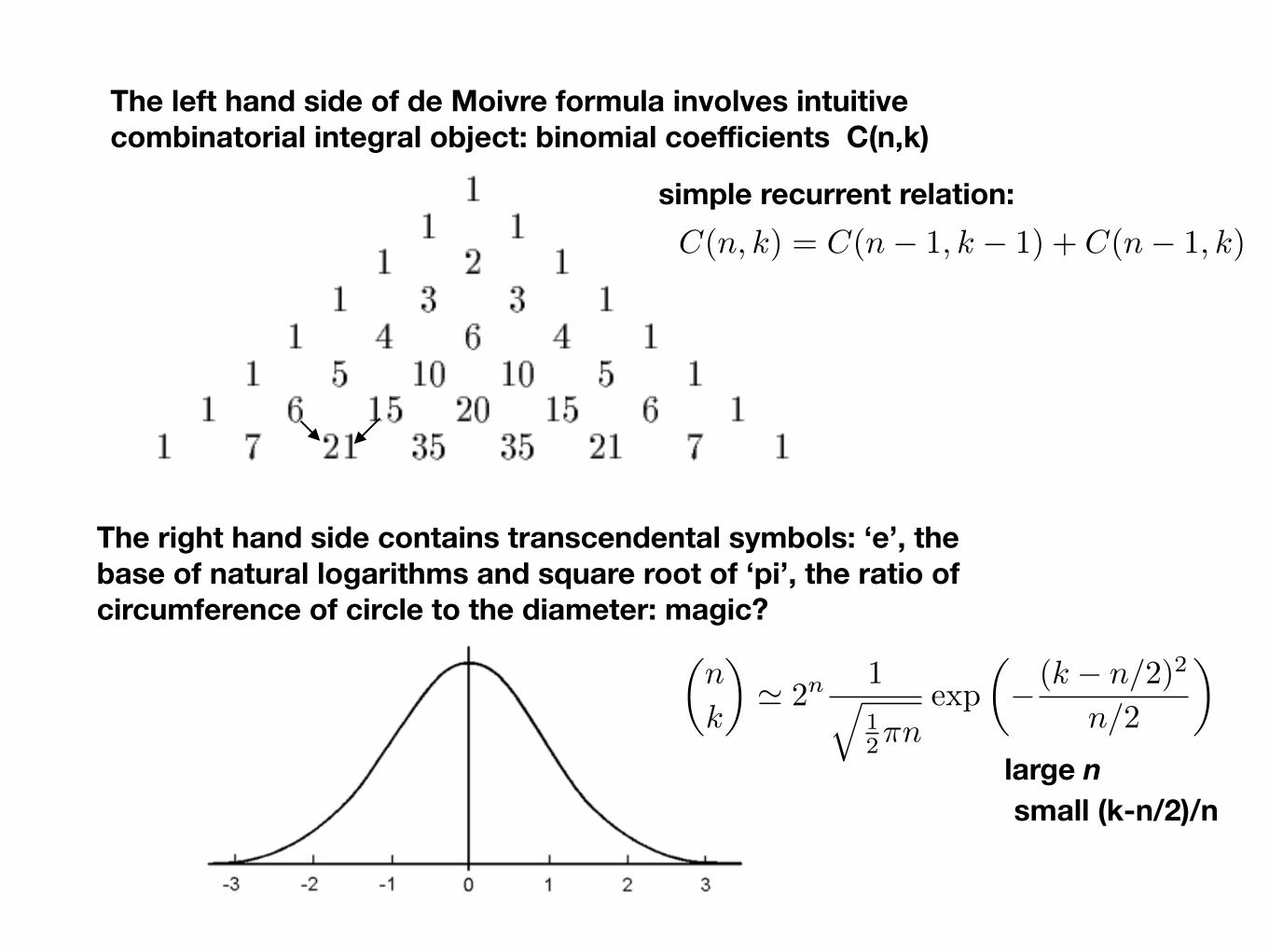
The left hand side of de Moivre formula involves intuitive combinatorial integral object: binomial coefficients C(n,k)

The right hand side contains transcendental symbols: ‘e’, the base of natural logarithms and square root of ‘pi’, the ratio of circumference of circle to the diameter: magic?

✓n

k

◆' 2n

1q12⇡n

exp

✓� (k � n/2)2

n/2

◆

C(n, k) = C(n� 1, k � 1) + C(n� 1, k)

simple recurrent relation:

large n small (k-n/2)/n

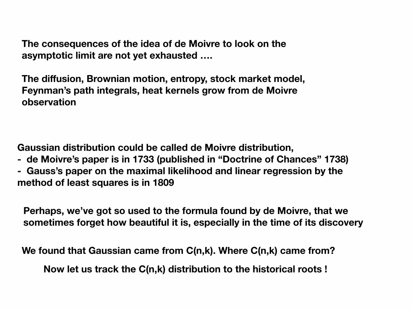
Perhaps, we’ve got so used to the formula found by de Moivre, that we sometimes forget how beautiful it is, especially in the time of its discovery

The consequences of the idea of de Moivre to look on the asymptotic limit are not yet exhausted ….

The diffusion, Brownian motion, entropy, stock market model, Feynman’s path integrals, heat kernels grow from de Moivre observation

Gaussian distribution could be called de Moivre distribution, - de Moivre’s paper is in 1733 (published in “Doctrine of Chances” 1738) - Gauss’s paper on the maximal likelihood and linear regression by the method of least squares is in 1809

Now let us track the C(n,k) distribution to the historical roots !

We found that Gaussian came from C(n,k). Where C(n,k) came from?

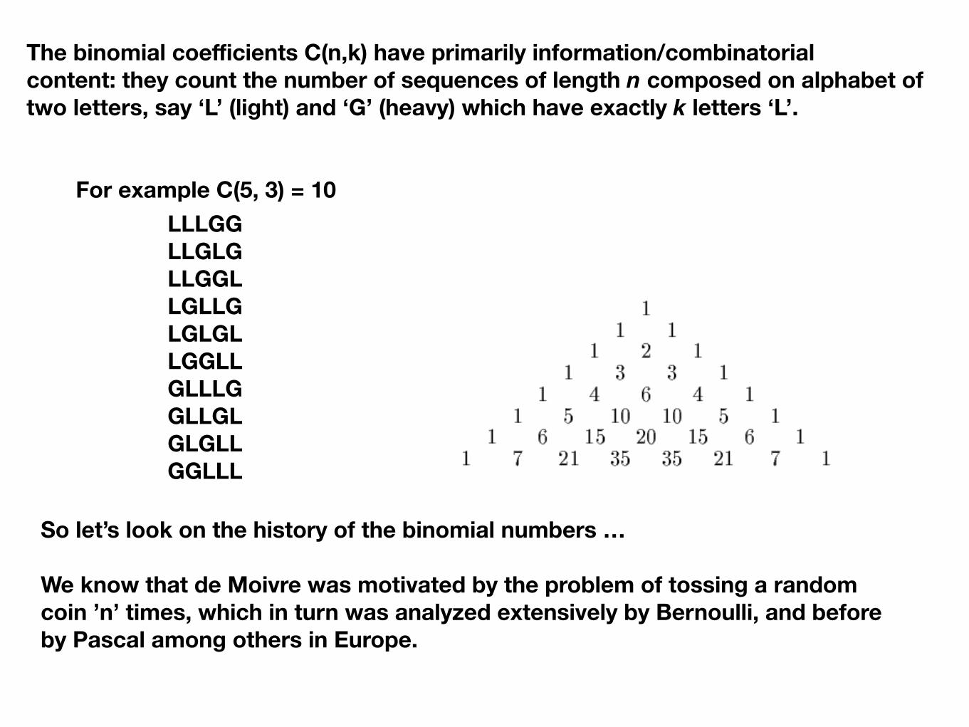
The binomial coefficients C(n,k) have primarily information/combinatorial content: they count the number of sequences of length n composed on alphabet of two letters, say ‘L’ (light) and ‘G’ (heavy) which have exactly k letters ‘L’.

For example C(5, 3) = 10LLLGG LLGLG LLGGL LGLLG LGLGL LGGLL GLLLG GLLGL GLGLL GGLLL

So let’s look on the history of the binomial numbers …

We know that de Moivre was motivated by the problem of tossing a random coin ’n’ times, which in turn was analyzed extensively by Bernoulli, and before by Pascal among others in Europe.

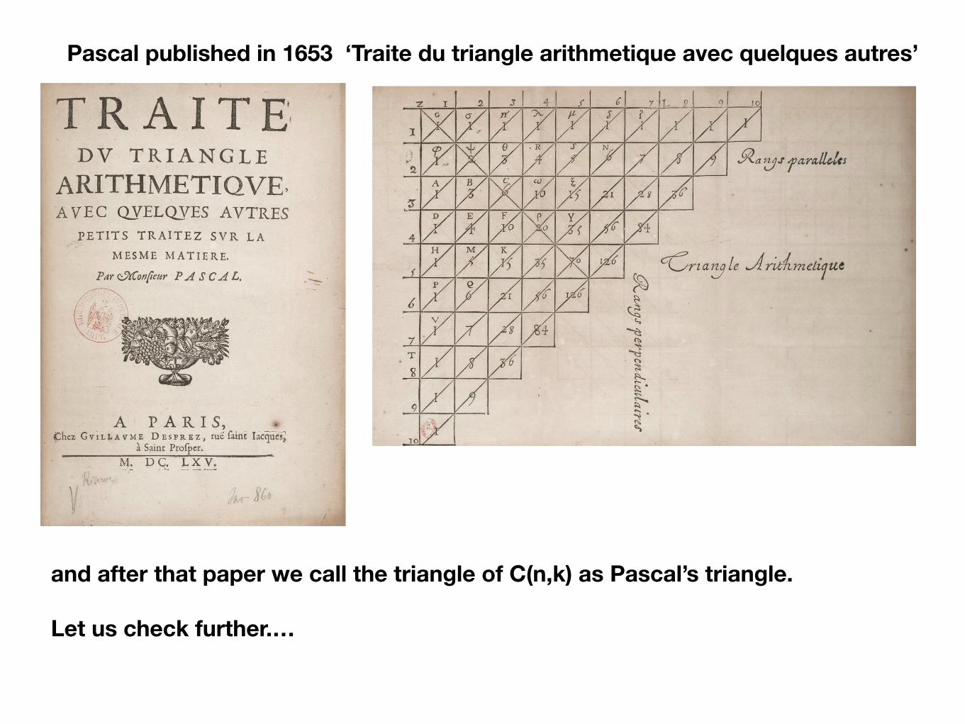
Pascal published in 1653 ‘Traite du triangle arithmetique avec quelques autres’

TRAITEDU TRIANGLE

ARITHMETIQUEAVEC QUELQUES AUTRESPETITS TRAITEZ SUR LA

MESME MATIERE.Monsieur PASCAL.

A PARIS,Chez GUILLAUME DESPREZ, rue saint Jacques,

M. DC. LXV.

and after that paper we call the triangle of C(n,k) as Pascal’s triangle.

Let us check further.…

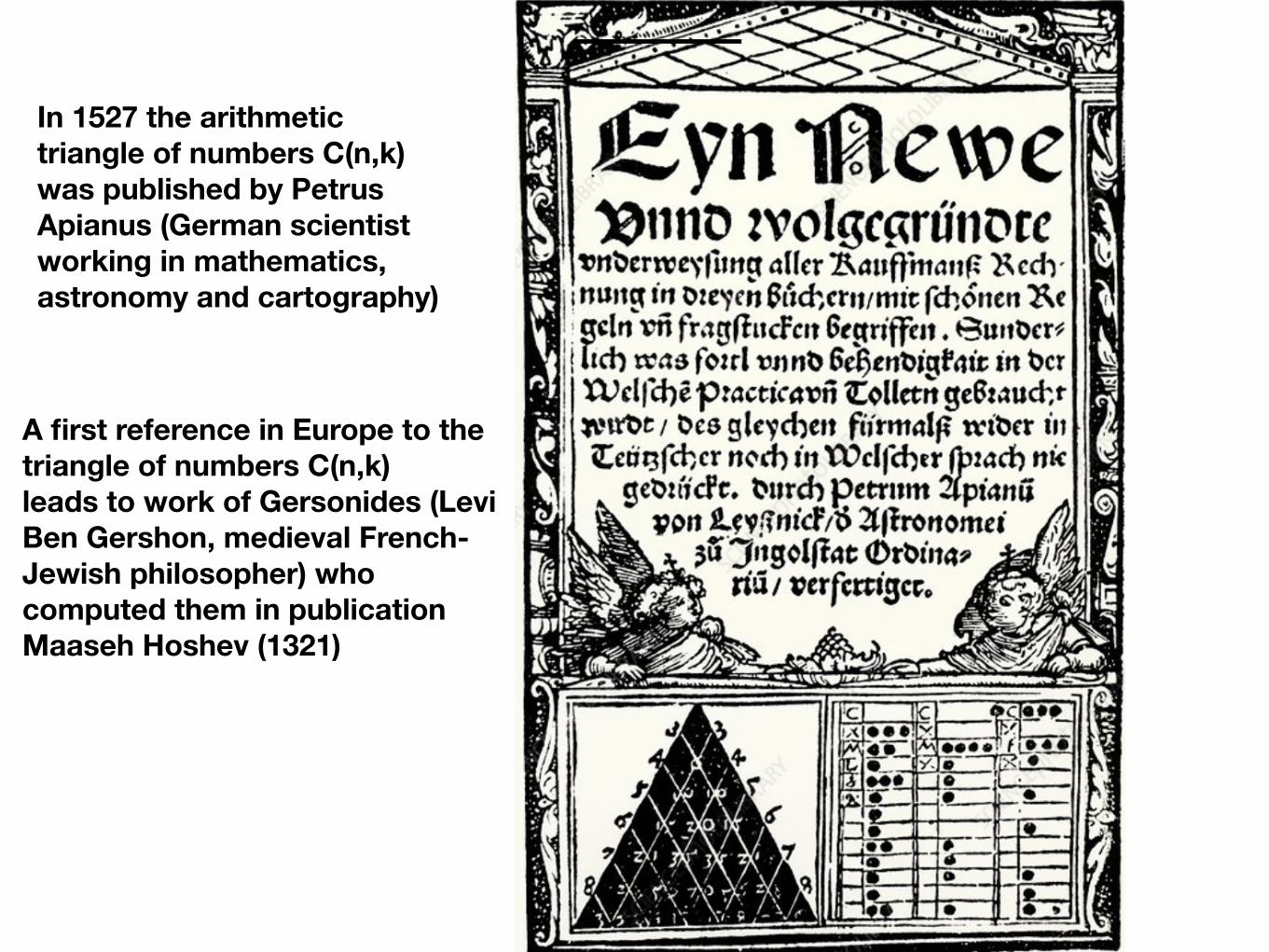
In 1527 the arithmetic triangle of numbers C(n,k) was published by Petrus Apianus (German scientist working in mathematics, astronomy and cartography)

A first reference in Europe to the triangle of numbers C(n,k) leads to work of Gersonides (Levi Ben Gershon, medieval French-Jewish philosopher) who computed them in publication Maaseh Hoshev (1321)

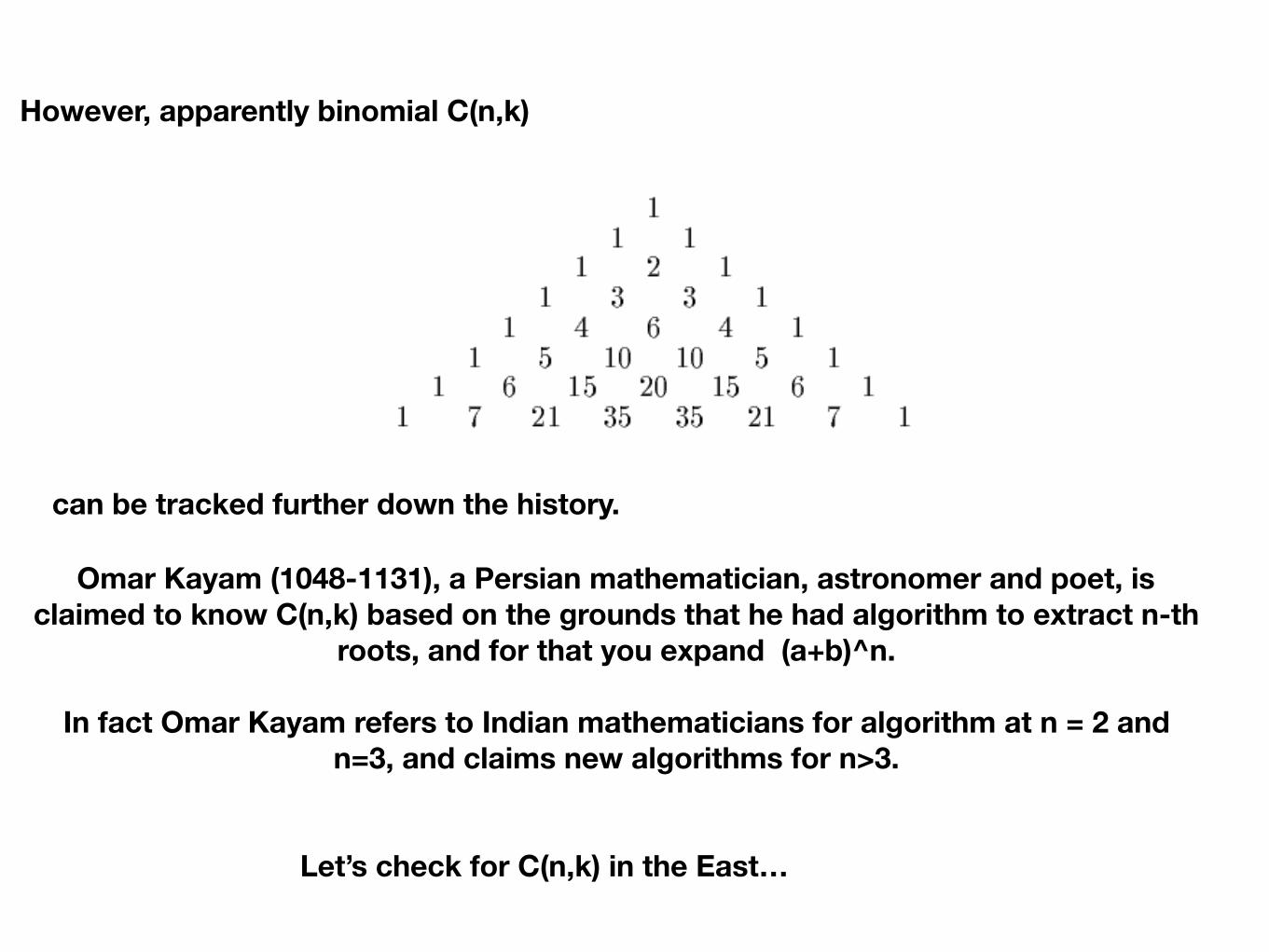
However, apparently binomial C(n,k)

can be tracked further down the history.

Omar Kayam (1048-1131), a Persian mathematician, astronomer and poet, is claimed to know C(n,k) based on the grounds that he had algorithm to extract n-th

roots, and for that you expand (a+b)^n.

In fact Omar Kayam refers to Indian mathematicians for algorithm at n = 2 and n=3, and claims new algorithms for n>3.

Let’s check for C(n,k) in the East…

In China the arithmetic triangle of C(n,k) is attributed to Jai Xian (1010-1070)

paper “Rújī Shìsuǒ” by mathematician Yang Hui (1238-1298) in his paper “Xiangjie Jiuzhang Suanfa” (1261).

The motivation of Yang Hui and Jai Xian seems to be the same as of Omar Kayam: give algorithms to extract n-th roots using binomial expansion of (a+b)^n

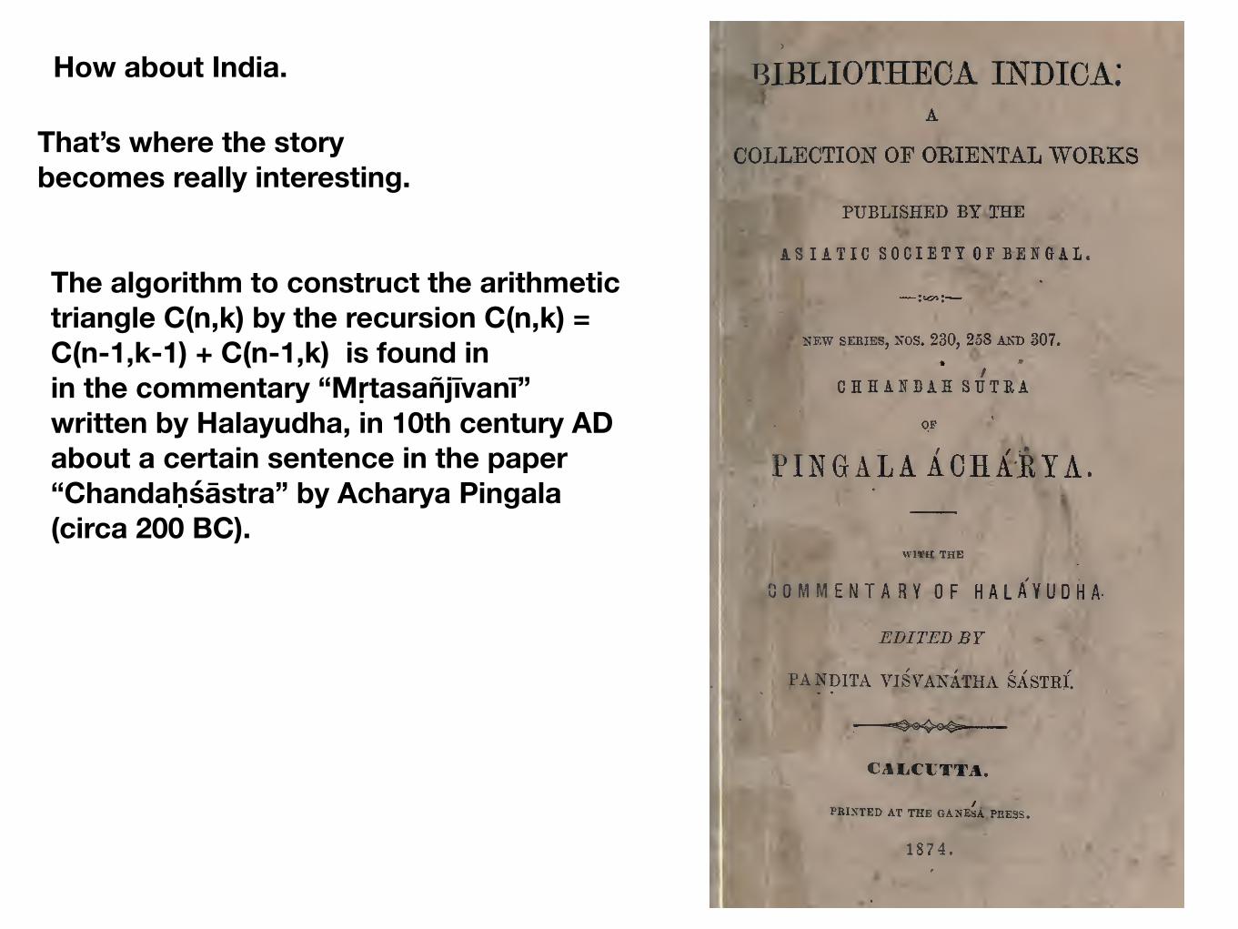
How about India.

That’s where the story becomes really interesting.

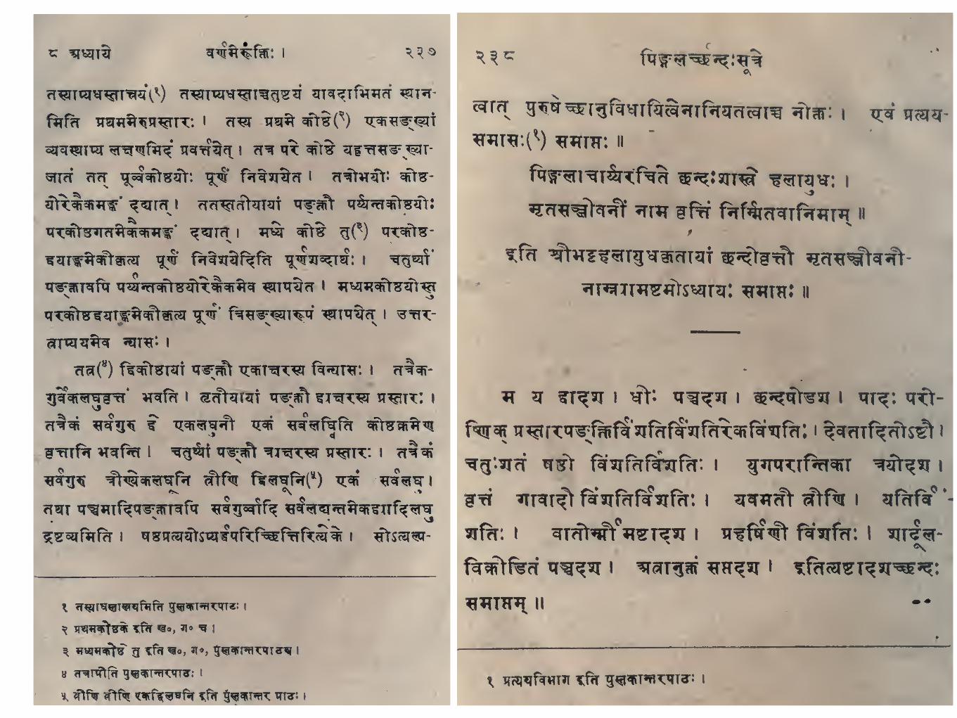
The algorithm to construct the arithmetic triangle C(n,k) by the recursion C(n,k) = C(n-1,k-1) + C(n-1,k) is found in in the commentary “Mṛtasañjīvanī” written by Halayudha, in 10th century AD about a certain sentence in the paper “Chandaḥśāstra” by Acharya Pingala (circa 200 BC).

BIBLIOTHEOA INDICA:A

COLLECTION OF OEIENTAL WORKS

PUBLISHED BY THE

ASIATIC SOCIETY OF BENGAL.

—:vc«:

—

NEW SEKIES, NOS. 230, 258 AKD 307.

CHHANDAH SUTRA

OF

PINGALAAOHlETA.

WIIH THE

OMMENTARY OF HALAYUDHA-

EDITED BY

PANDITA VISVANATHA SASTRI.

CAE.CUTTA.

PRINTED AT THE GANEsA PRESS.

1874,

So who is Pingala in 1st-2nd century BC in India and what was the problem he was trying to solve ?

In the modern language Pingala was information theorist worked on the coding theory.

The language of the time was Sanskrit, and substantial portion of the literature was the poetry. Almost all of Sanskrit poetry is based on following of the certain meter or arrangement of syllables. Prosody is the study of meter.

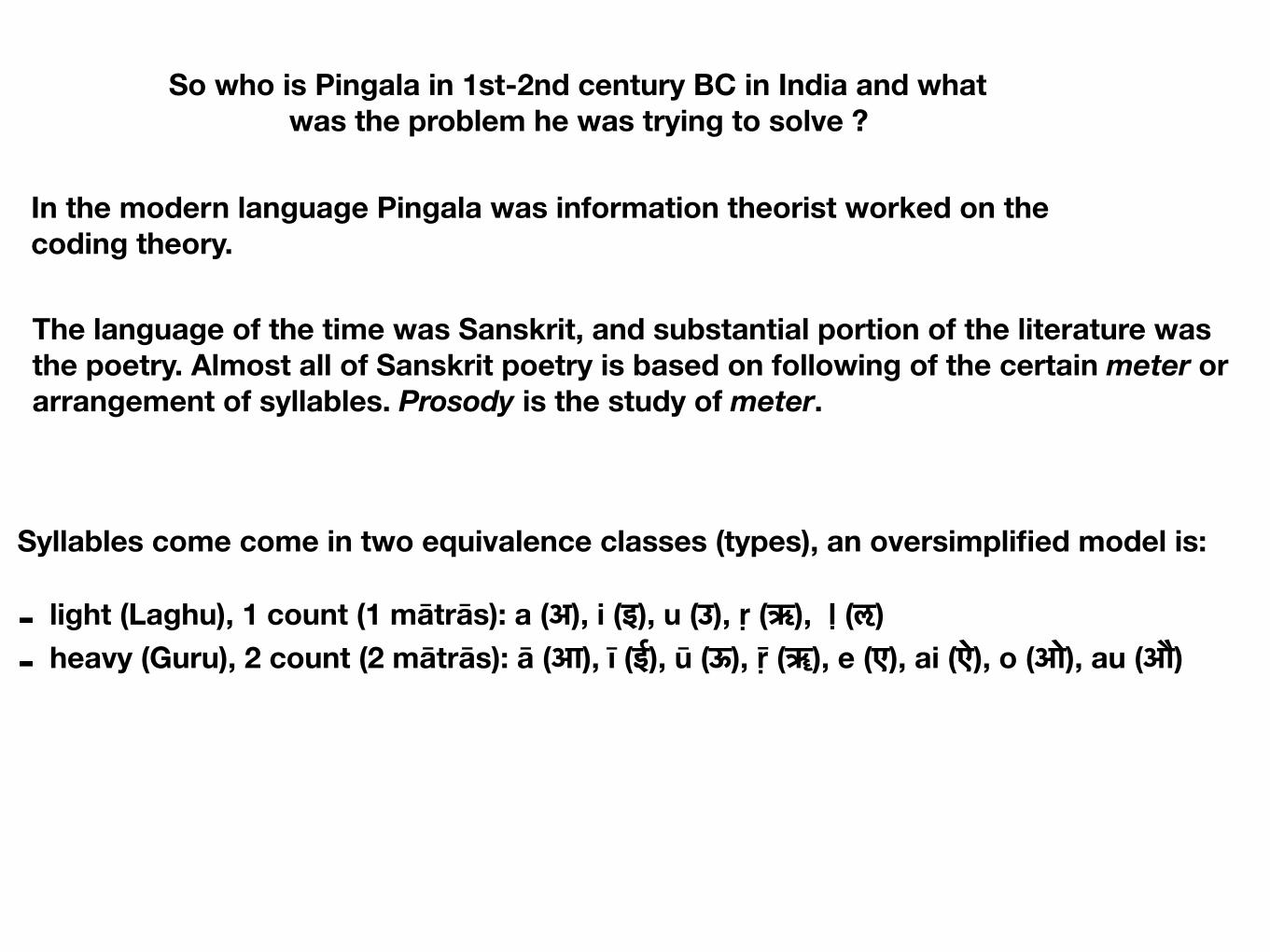
Syllables come come in two equivalence classes (types), an oversimplified model is:

- light (Laghu), 1 count (1 mātrās): a (अ), i (इ), u (उ), ṛ (ऋ), ḷ (ऌ) - heavy (Guru), 2 count (2 mātrās): ā (आ), ī (ई), ū (ऊ), ṝ (ॠ), e (ए), ai (ऐ), o (ओ), au (औ)

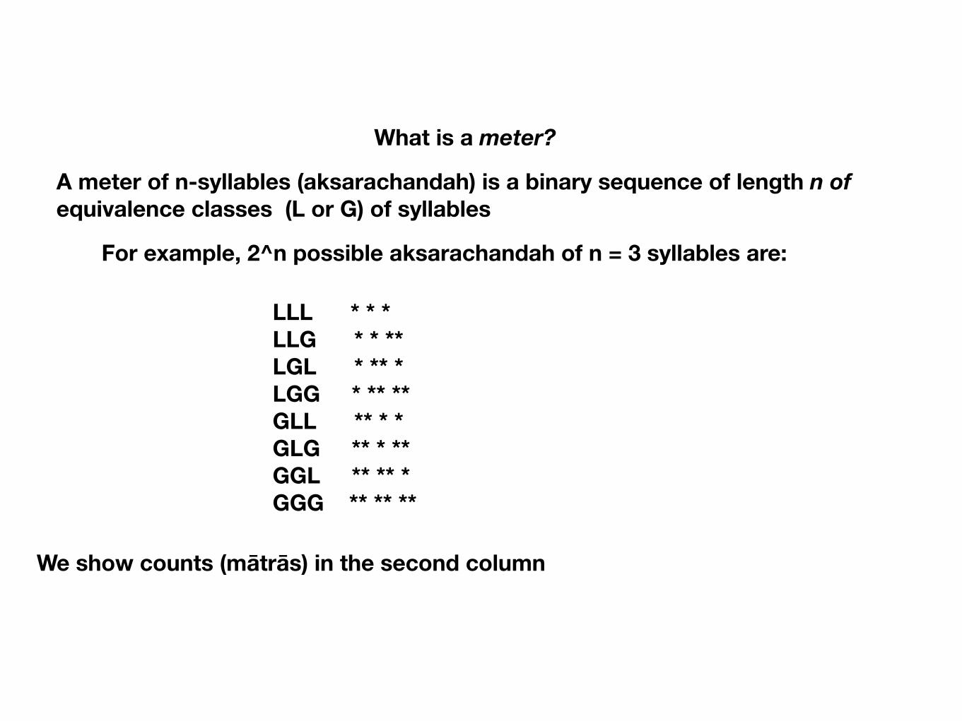
What is a meter?

A meter of n-syllables (aksarachandah) is a binary sequence of length n of equivalence classes (L or G) of syllables

For example, 2^n possible aksarachandah of n = 3 syllables are:

LLL * * * LLG * * ** LGL * ** * LGG * ** ** GLL ** * * GLG ** * ** GGL ** ** * GGG ** ** **

We show counts (mātrās) in the second column

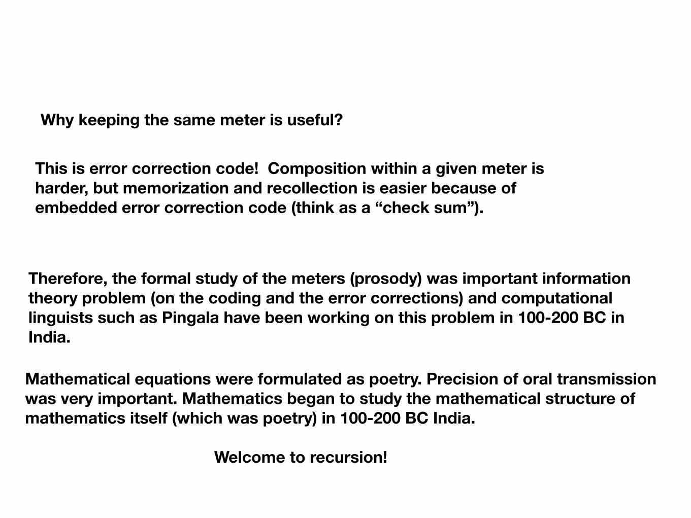
Why keeping the same meter is useful?

This is error correction code! Composition within a given meter is harder, but memorization and recollection is easier because of embedded error correction code (think as a “check sum”).

Therefore, the formal study of the meters (prosody) was important information theory problem (on the coding and the error corrections) and computational linguists such as Pingala have been working on this problem in 100-200 BC in India.

Mathematical equations were formulated as poetry. Precision of oral transmission was very important. Mathematics began to study the mathematical structure of mathematics itself (which was poetry) in 100-200 BC India.

Welcome to recursion!

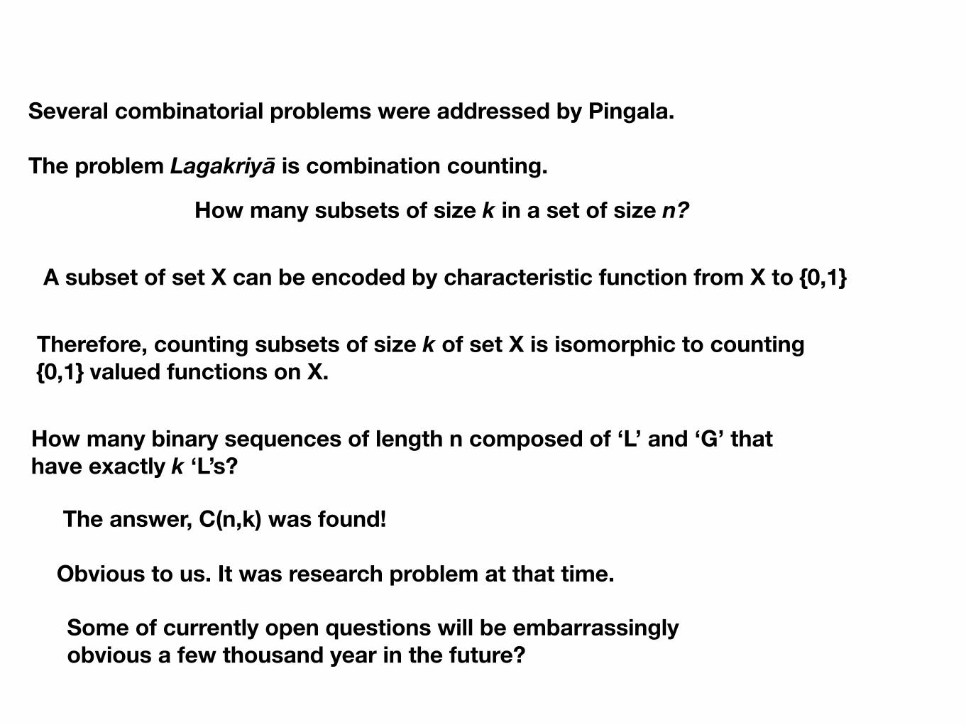
Several combinatorial problems were addressed by Pingala.

The problem Lagakriyā is combination counting.

How many binary sequences of length n composed of ‘L’ and ‘G’ that have exactly k ‘L’s?

How many subsets of size k in a set of size n?

A subset of set X can be encoded by characteristic function from X to {0,1}

Therefore, counting subsets of size k of set X is isomorphic to counting {0,1} valued functions on X.

The answer, C(n,k) was found!

Obvious to us. It was research problem at that time.

Some of currently open questions will be embarrassingly obvious a few thousand year in the future?

«\

(^"'^

) fl[^^^'fI^'flT5!W, II^J^ II

O q^^ T^m II ^^ II

ft^f^rf ^T^ W^"^ iTfT^t ^^^^T ^^fh I rl^^T I

'^g'.^f^^^^ ^^iTTT^t ^^<55T(^) ^^f^m ^?rt

C^'^) q^ qtofiifrT II ^o II

8 ^^^f^ffj ^', •g^'^T'fiTtn^^ 1

«\

(^"'^

) fl[^^^'fI^'flT5!W, II^J^ II

O q^^ T^m II ^^ II

ft^f^rf ^T^ W^"^ iTfT^t ^^^^T ^^fh I rl^^T I

'^g'.^f^^^^ ^^iTTT^t ^^<55T(^) ^^f^m ^?rt

C^'^) q^ qtofiifrT II ^o II

8 ^^^f^ffj ^', •g^'^T'fiTtn^^ 1

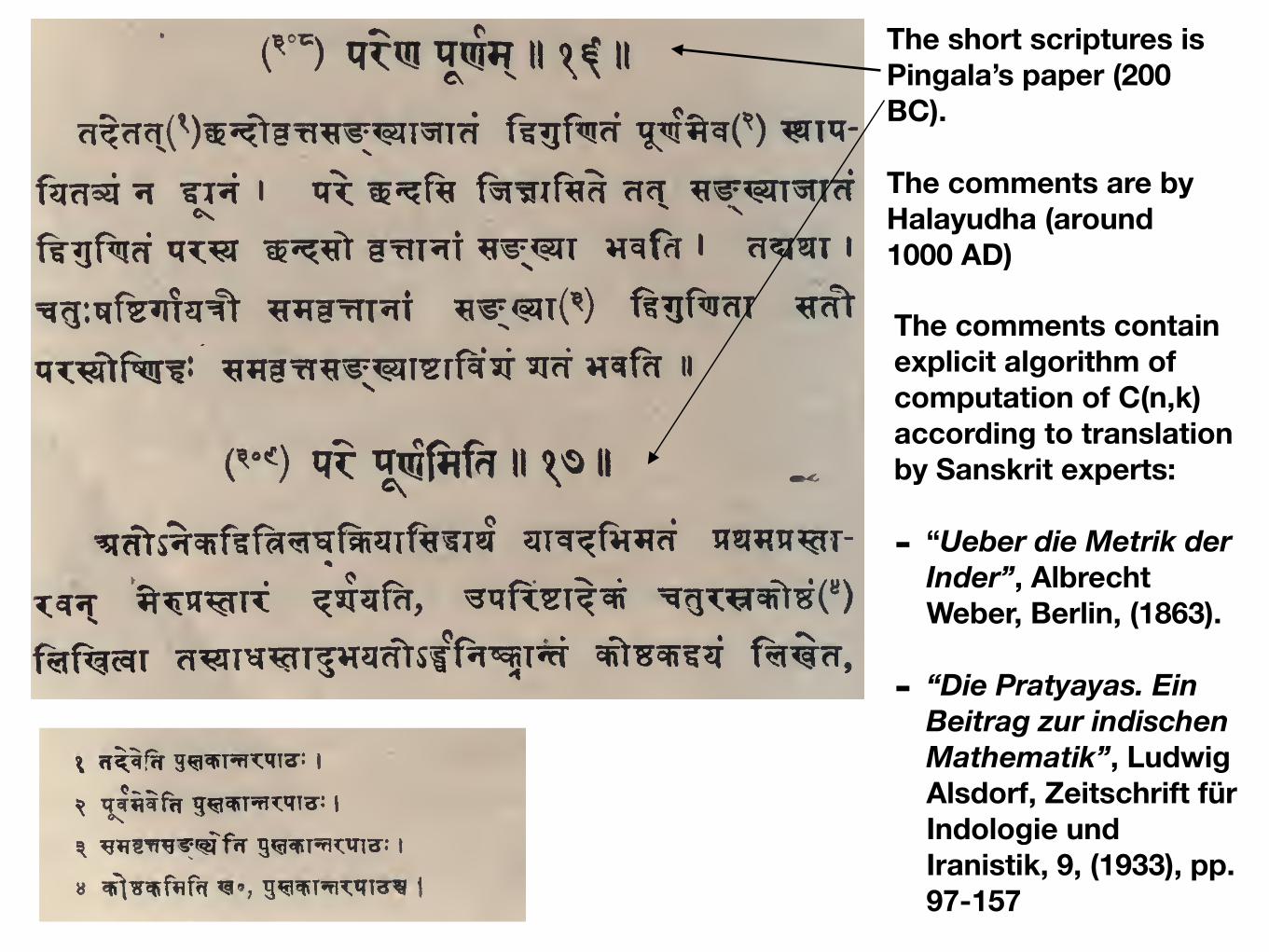
The short scriptures is Pingala’s paper (200 BC).

The comments are by Halayudha (around 1000 AD)

The comments contain explicit algorithm of computation of C(n,k) according to translation by Sanskrit experts:

- “Ueber die Metrik der Inder”, Albrecht Weber, Berlin, (1863).

- “Die Pratyayas. Ein Beitrag zur indischen Mathematik”, Ludwig Alsdorf, Zeitschrift für Indologie und Iranistik, 9, (1933), pp. 97-157

I

sji^^Txir ^rg'nf^^* Ti^^tcT I fi^ ^T ^r§ ^itt^^^^t-

^T€t^7T<T%^T^mif* ^^mi ^ ^i ^0) ^T^^-

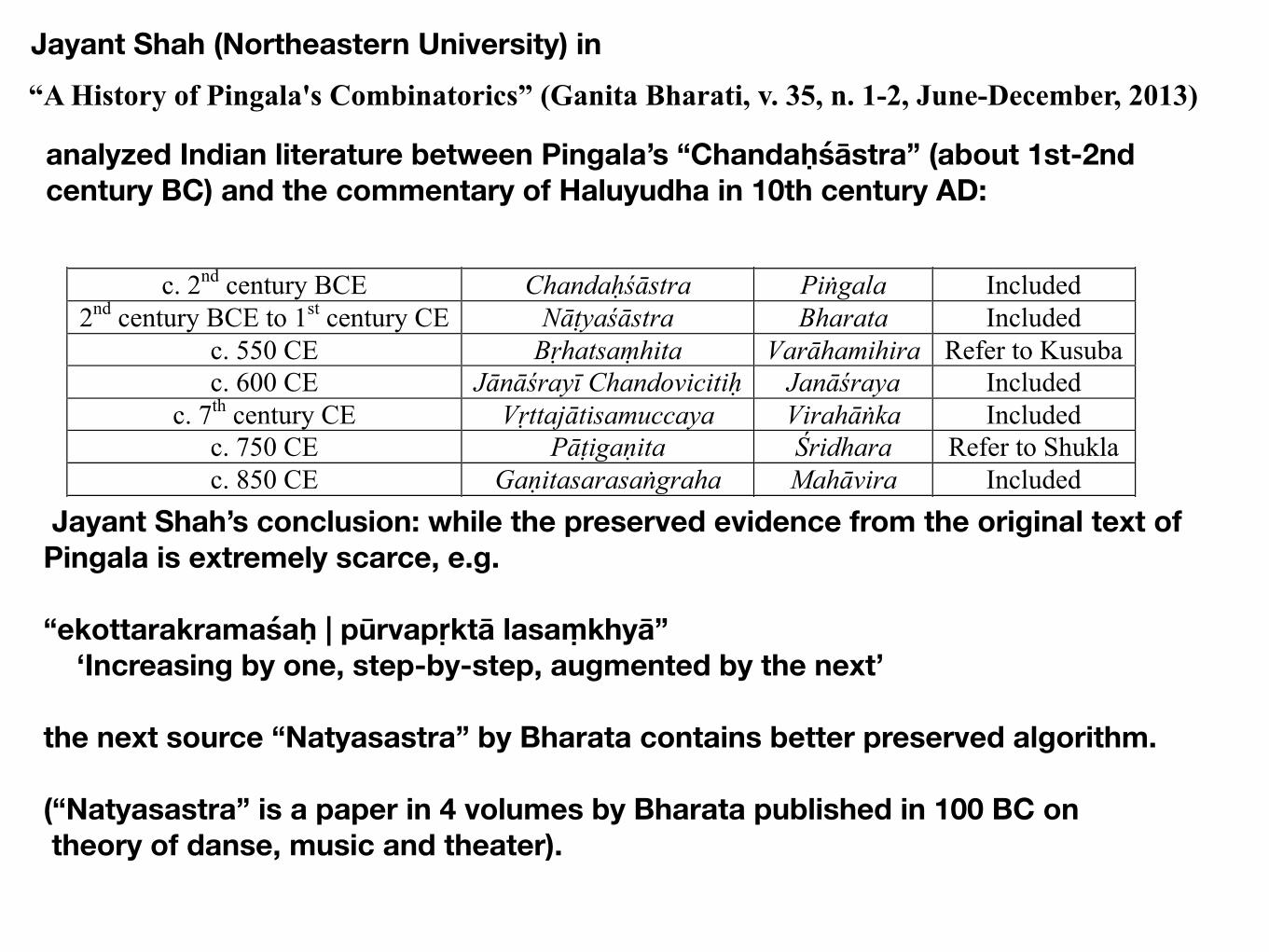
“A History of Pingala's Combinatorics” (Ganita Bharati, v. 35, n. 1-2, June-December, 2013)

Jayant Shah (Northeastern University) in

analyzed Indian literature between Pingala’s “Chandaḥśāstra” (about 1st-2nd century BC) and the commentary of Haluyudha in 10th century AD:

! 3!

masters and the construction must go back to Piṅgala. None of the prosodists following Piṅgala acknowledges Bharata, but they do acknowledge Piṅgala. This paper systematically traces Piṅgala’s algorithms through the Indian mathematical literature over the course of one and a half millennia. It finds no evidence to support Halāyudha’s interpretation of Piṅgala’s last sūtra, but still traces the computation of the binomial coefficients to Piṅgala. Especially relevant are the compositions of Bharata and Janāśraya which are chronologically closest to Piṅgala. The section on Sanskrit meters in Bharata’s Nāṭyaśāstra (composed sometime between 2nd century BCE and 1st century CE) still has not been translated. Words are corrupted here and there and some of verses appear out of order. Regnaud4 in his monograph on Bharata’s exposition on prosody concedes that a literal translation is not possible and skips many verses without attempting even a loose interpretation. In his 1933 paper on combinatorics in Hemacandra’s Chandonuśasanam, Alsdorf establishes a loose correspondence between Bharata and Hemacandra without translating Nāṭyaśāstra. The Sanskrit commentary of Abhinavagupta (c. 1000 CE) on Nāṭyaśāstra is spotty and frequently substitutes equivalent algorithms from later sources instead of explaining the actual verse. Jānāśrayi of Janāśraya (c. 6th century CE) is absent from the literature on Piṅgala’s combinatorics. Even in his otherwise excellent summary of Indian combinatorics before Nārāyaṇa, Kusuba barely mentions Bharata and does not mention Janāśraya. In this paper, we give translations of both works. Even in places where the literal text is unclear, its mathematical content is unambiguous. We also give translations of Vṛttajātisamuccaya of Virahāṅka, Jayadevacchandaḥ of Jayadeva, Chandonuśasanaṃ of Jayakīrti and Vṛttaratnākara of Kedāra which have not yet been translated into a western language. In the case of Vṛttajātisamuccaya, which was composed by Virahāṅka in Prākṛta, only its Sanskrit version rendered by his commentator is given. The survey in this paper is based on the following primary sources:

Date Title Author Translation c. 2nd century BCE Chandaḥśāstra Piṅgala Included

2nd century BCE to 1st century CE Nāṭyaśāstra Bharata Included c. 550 CE Bṛhatsaṃhita Varāhamihira Refer to Kusuba c. 600 CE Jānāśrayī Chandovicitiḥ Janāśraya Included

c. 7th century CE Vṛttajātisamuccaya Virahāṅka Included c. 750 CE Pāṭigaṇita Śridhara Refer to Shukla c. 850 CE Gaṇitasarasaṅgraha Mahāvira Included

before 900 CE Jayadevacchandaḥ Jayadeva Included c. 950 CE Mṛtasañjīvanī Halāyudha Refer to Weber c. 1000 CE Chandonuśasanaṃ Jayakīrti Included c. 1100 CE Vṛttaratnākara Kedāra Included c. 1150 CE Chandonuśasanam Hemacandra Included 1356 CE Gaṇitakaumudi Nārāyaṇa Refer to Kusuba Unknown Ratnamañjūṣa Unknown Refer to Kusuba

!!!!!!!!!!!!!!!!!!!!!!!!!!!!!!!!!!!!!!!!!!!!!!!!!!!!!!!!!!!!!

4!“La Métrique de Bharata”, Paul Regnaud, Extrait des annals du musée guimet, v. 2, Paris, (1880).

Jayant Shah’s conclusion: while the preserved evidence from the original text of Pingala is extremely scarce, e.g.

“ekottarakramaśaḥ | pūrvapṛktā lasaṃkhyā” ‘Increasing by one, step-by-step, augmented by the next’

the next source “Natyasastra” by Bharata contains better preserved algorithm.

(“Natyasastra” is a paper in 4 volumes by Bharata published in 100 BC on theory of danse, music and theater).

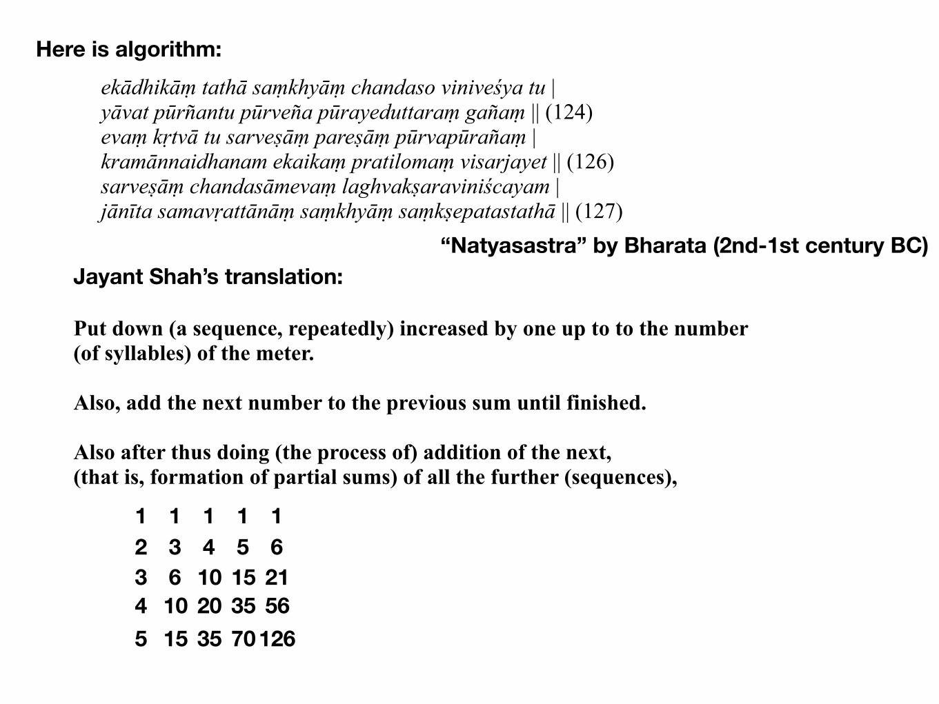
ekādhikāṃ tathā saṃkhyāṃ chandaso viniveśya tu | yāvat pūrñantu pūrveña pūrayeduttaraṃ gañaṃ || (124) evaṃ kṛtvā tu sarveṣāṃ pareṣāṃ pūrvapūrañaṃ | kramānnaidhanam ekaikaṃ pratilomaṃ visarjayet || (126) sarveṣāṃ chandasāmevaṃ laghvakṣaraviniścayam | jānīta samavṛattānāṃ saṃkhyāṃ saṃkṣepatastathā || (127)

Jayant Shah’s translation:

Put down (a sequence, repeatedly) increased by one up to to the number (of syllables) of the meter.

Also, add the next number to the previous sum until finished.

Also after thus doing (the process of) addition of the next, (that is, formation of partial sums) of all the further (sequences),

12345

1361015

14102035

15153570

162156

126

“Natyasastra” by Bharata (2nd-1st century BC)

Here is algorithm:

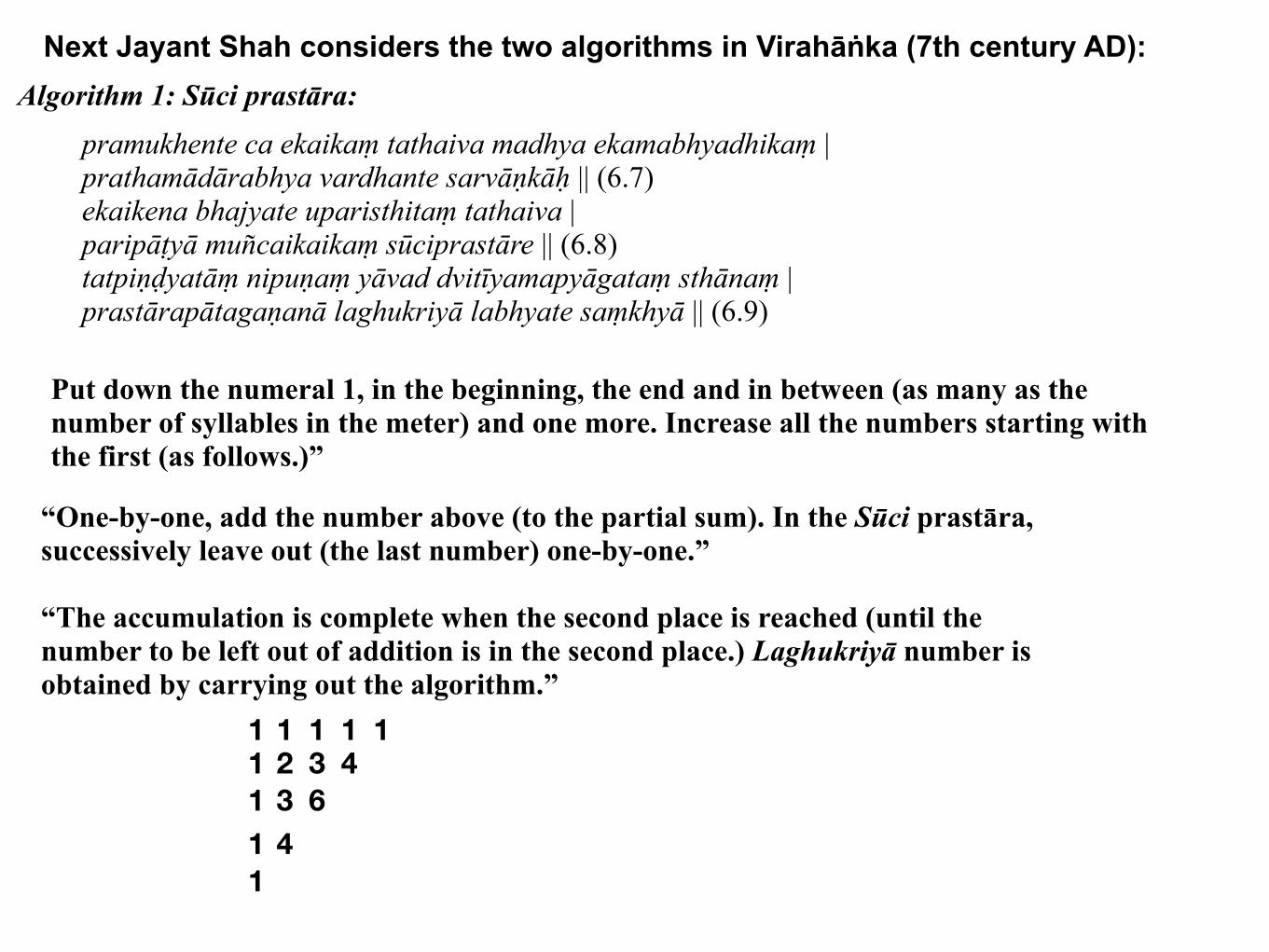
Next Jayant Shah considers the two algorithms in Virahāṅka (7th century AD):

pramukhente ca ekaikaṃ tathaiva madhya ekamabhyadhikaṃ | prathamādārabhya vardhante sarvāṇkāḥ || (6.7) ekaikena bhajyate uparisthitaṃ tathaiva | paripāṭyā muñcaikaikaṃ sūciprastāre || (6.8) tatpiṇḍyatāṃ nipuṇaṃ yāvad dvitīyamapyāgataṃ sthānaṃ | prastārapātagaṇanā laghukriyā labhyate saṃkhyā || (6.9)

Put down the numeral 1, in the beginning, the end and in between (as many as the number of syllables in the meter) and one more. Increase all the numbers starting with the first (as follows.)”

“One-by-one, add the number above (to the partial sum). In the Sūci prastāra, successively leave out (the last number) one-by-one.”

“The accumulation is complete when the second place is reached (until the number to be left out of addition is in the second place.) Laghukriyā number is obtained by carrying out the algorithm.”

11111

1234

136

14

1

Algorithm 1: Sūci prastāra:

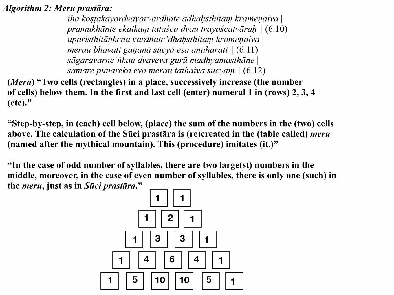
(Meru) “Two cells (rectangles) in a place, successively increase (the number of cells) below them. In the first and last cell (enter) numeral 1 in (rows) 2, 3, 4 (etc).”

“Step-by-step, in (each) cell below, (place) the sum of the numbers in the (two) cells above. The calculation of the Sūci prastāra is (re)created in the (table called) meru (named after the mythical mountain). This (procedure) imitates (it.)”

“In the case of odd number of syllables, there are two large(st) numbers in the middle, moreover, in the case of even number of syllables, there is only one (such) in the meru, just as in Sūci prastāra.”

Algorithm 2: Meru prastāra:iha koṣṭakayordvayorvardhate adhaḥsthitaṃ krameṇaiva | pramukhānte ekaikaṃ tataśca dvau trayaścatvāraḥ || (6.10) uparisthitāṅkena vardhate’dhaḥsthitaṃ krameṇaiva | merau bhavati gaṇanā sūcyā eṣa anuharati || (6.11) sāgaravarṇe’ṅkau dvaveva gurū madhyamasthāne | samare punareka eva merau tathaiva sūcyāṃ || (6.12)

1 1

1 1

1 1

1 1

1 1

2

3 3

4 6 4

5 10 10 5

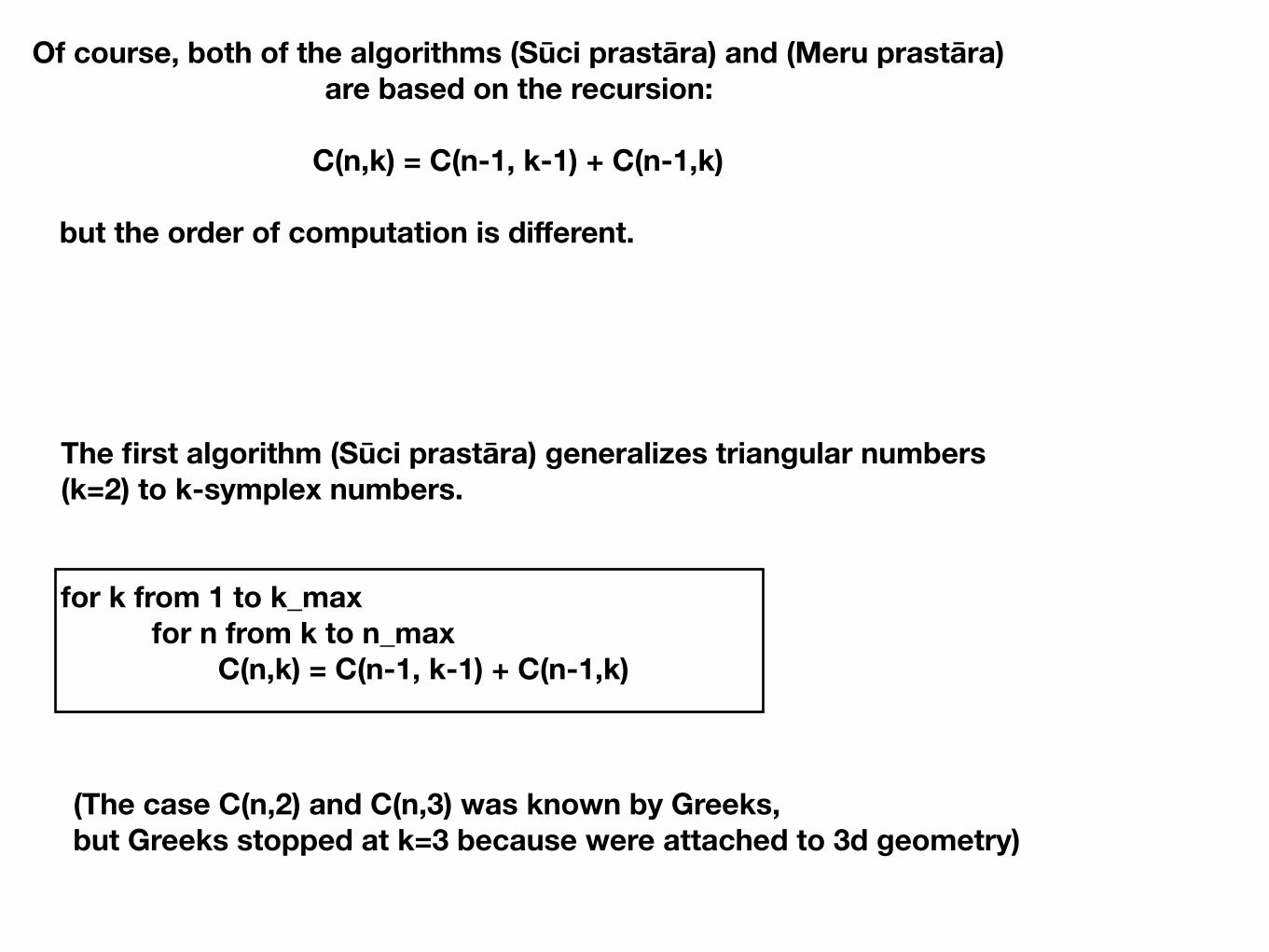
Of course, both of the algorithms (Sūci prastāra) and (Meru prastāra) are based on the recursion:

C(n,k) = C(n-1, k-1) + C(n-1,k)

but the order of computation is different.

The first algorithm (Sūci prastāra) generalizes triangular numbers (k=2) to k-symplex numbers.

for k from 1 to k_max for n from k to n_max C(n,k) = C(n-1, k-1) + C(n-1,k)

(The case C(n,2) and C(n,3) was known by Greeks, but Greeks stopped at k=3 because were attached to 3d geometry)

The second algorithm (Meru prastara) is what actually leads to random walk, Gaussian distribution, central limit theorem, Markov processes, heat kernel and finally to the path integral of quantum field theory.

for n from 1 to n_max for k from 1 to n-1

C(n,k) = C(n-1, k-1) + C(n-1,k)

The recursionC(n,k) = C(n-1, k-1) + C(n-1,k)

is a discrete (difference) version of the heat (diffusion) equation, whose solution is the heat kernel in time ’n’ and space ‘k’. This is one of ways to derive Gaussian from Meru prastaara C(n,k) taking large n.

In continuous limit, if time ’n’ is further multiplied by square root of -1 (Wick rotation) we get Schröedinger equation on 1d particle moving on line ‘k’ and Feynman’s formulation of quantum mechanics.

It is wonderful that the first work of information theorists (poets) in India from 200 BC to 700 AD names

C(n,k) / discrete Gaussian / heat kernel as Meru-prastaara “Mount Meru” which was considered to be the center of

all physical, metaphysical and spiritual universes.

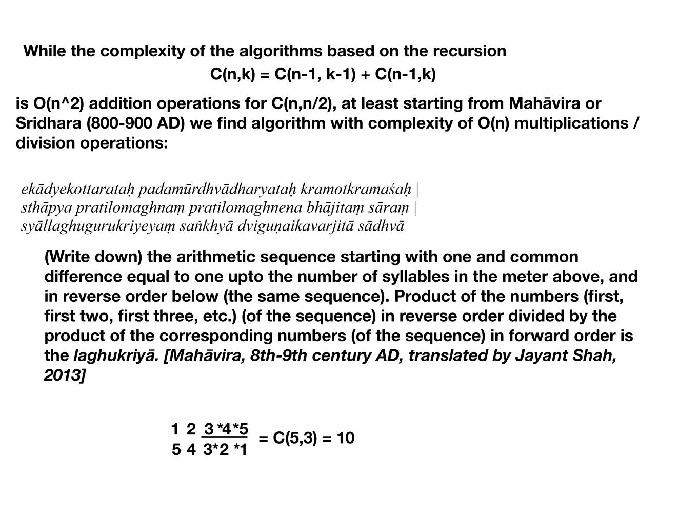
While the complexity of the algorithms based on the recursion C(n,k) = C(n-1, k-1) + C(n-1,k)

is O(n^2) addition operations for C(n,n/2), at least starting from Mahāvira or Sridhara (800-900 AD) we find algorithm with complexity of O(n) multiplications / division operations: ekādyekottarataḥ padamūrdhvādharyataḥ kramotkramaśaḥ | sthāpya pratilomaghnaṃ pratilomaghnena bhājitaṃ sāraṃ | syāllaghugurukriyeyaṃ saṅkhyā dviguṇaikavarjitā sādhvā

(Write down) the arithmetic sequence starting with one and common difference equal to one upto the number of syllables in the meter above, and in reverse order below (the same sequence). Product of the numbers (first, first two, first three, etc.) (of the sequence) in reverse order divided by the product of the corresponding numbers (of the sequence) in forward order is the laghukriyā. [Mahāvira, 8th-9th century AD, translated by Jayant Shah, 2013]

1 2 3 4 5 12345**** = C(5,3) = 10

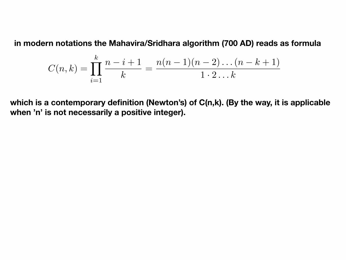
C(n, k) =kY

i=1

n� i+ 1

k=

n(n� 1)(n� 2) . . . (n� k + 1)

1 · 2 . . . k

in modern notations the Mahavira/Sridhara algorithm (700 AD) reads as formula

which is a contemporary definition (Newton’s) of C(n,k). (By the way, it is applicable when ’n’ is not necessarily a positive integer).

C(n, k) =

✓n

k

◆=

n!

k!(n� k)!

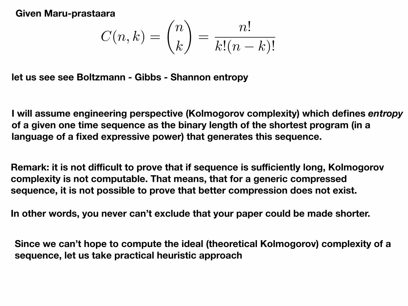
let us see see Boltzmann - Gibbs - Shannon entropy

I will assume engineering perspective (Kolmogorov complexity) which defines entropy of a given one time sequence as the binary length of the shortest program (in a language of a fixed expressive power) that generates this sequence.

Remark: it is not difficult to prove that if sequence is sufficiently long, Kolmogorov complexity is not computable. That means, that for a generic compressed sequence, it is not possible to prove that better compression does not exist.

In other words, you never can’t exclude that your paper could be made shorter.

Since we can’t hope to compute the ideal (theoretical Kolmogorov) complexity of a sequence, let us take practical heuristic approach

Given Maru-prastaara

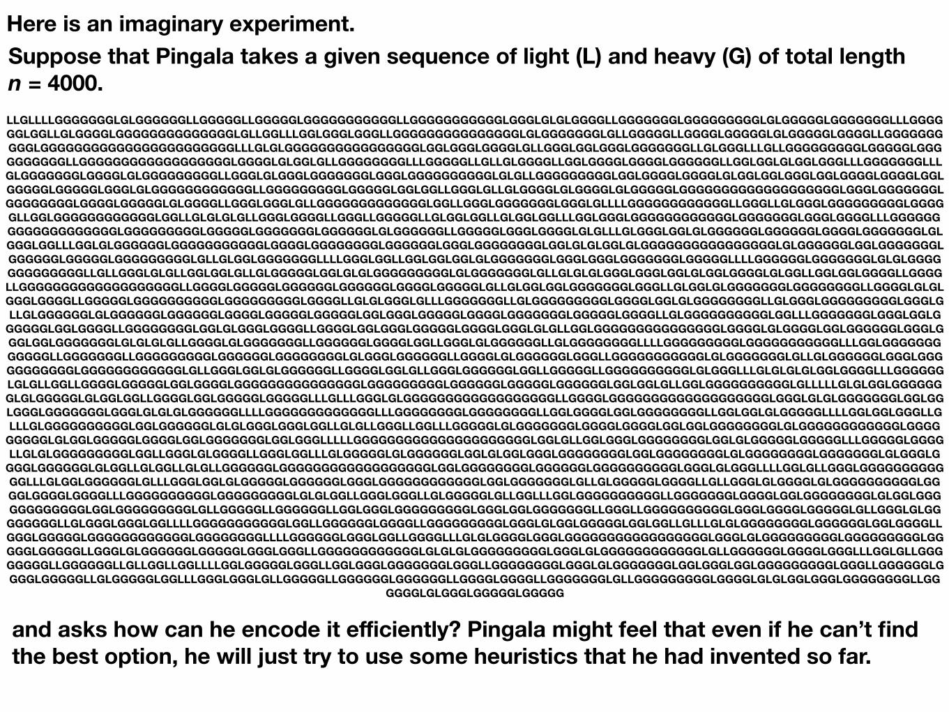
Suppose that Pingala takes a given sequence of light (L) and heavy (G) of total length n = 4000.LLGLLLLGGGGGGGLGLGGGGGGLLGGGGGLLGGGGGLGGGGGGGGGGGLLGGGGGGGGGGGLGGGLGLGLGGGGLLGGGGGGGLGGGGGGGGGLGLGGGGGLGGGGGGGLLLGGGGGGLGGLLGLGGGGLGGGGGGGGGGGGGGLGLLGGLLLGGLGGGLGGGLLGGGGGGGGGGGGGGGLGLGGGGGGGLGLLGGGGGLLGGGGLGGGGGLGLGGGGGLGGGGLLGGGGGGGGGGLGGGGGGGGGGGGGGGGGGGGGGGLLLGLGLGGGGGGGGGGGGGGGGLGGLGGGLGGGGLGLLGGGLGGLGGGLGGGGGGGLLGLGGGLLLGLLGGGGGGGGGLGGGGGLGGGGGGGGGGLLGGGGGGGGGGGGGGGGGGLGGGGLGLGGLGLLGGGGGGGGLLLGGGGGLLGLLGLGGGGLLGGLGGGGLGGGGLGGGGGGLLGGLGGLGLGGLGGGLLLGGGGGGGLLLGLGGGGGGGLGGGGLGLGGGGGGGGGLLGGGLGLGGGLGGGGGGGLGGGLGGGGGGGGGGLGLGLLGGGGGGGGGLGGLGGGGLGGGGLGLGGLGGLGGGLGGLGGGGLGGGGLGGLGGGGGLGGGGGLGGGLGLGGGGGGGGGGGGLLGGGGGGGGGLGGGGGLGGLGGLLGGGLGLLGLGGGGLGLGGGGLGLGGGGGLGGGGGGGGGGGGGGGGGGGLGGGLGGGGGGGLGGGGGGGGLGGGGLGGGGGLGLGGGGLLGGGLGGGLGLLGGGGGGGGGGGGGLGGLLGGGLGGGGGGGLGGGLGLLLLGGGGGGGGGGGGLLGGGLLGLGGGLGGGGGGGGGLGGGGGLLGGLGGGGGGGGGGGGLGGLLGLGLGLGLLGGGLGGGGLLGGGLLGGGGGLLGLGGLGGLLGLGGLGGLLLGGLGGGLGGGGGGGGGGGGLGGGGGGGLGGGLGGGGLLLGGGGGGGGGGGGGGGGGGGLGGGGGGGGGLGGGGGLGGGGGGGLGGGGGGLGLGGGGGGLLGGGGGLGGGLGGGGLGLGLLLGLGGGLGGLGLGGGGGGLGGGGGGLGGGGLGGGGGGGLGLGGGLGGLLLGGLGLGGGGGGLGGGGGGGGGGGLGGGGLGGGGGGGGLGGGGGGLGGGLGGGGGGGGLGGLGLGLGGLGLGGGGGGGGGGGGGGGGLGLGGGGGGLGGLGGGGGGGLGGGGGGLGGGGGLGGGGGGGGGLGLLGLGGLGGGGGGGLLLLGGGLGGLLGGLGGLGGLGLGGGGGGGLGGGLGGGLGGGGGGGLGGGGGLLLLGGGGGGLGGGGGGGLGLGLGGGGGGGGGGGGGLLGLLGGGLGLGLLGGLGGLGLLGLGGGGGLGGLGLGLGGGGGGGGGLGLGGGGGGGLGLLGLGLGLGGGLGGGLGGLGLGGLGGGGLGLGGLLGGLGGLGGGGLLGGGGLLGGGGGGGGGGGGGGGGGGGLLGGGGLGGGGGLGGGGGGLGGGGGGLGGGGLGGGGGLGLLGLGGLGGLGGGGGGGLGGGLLGLGGLGLGGGGGGGLGGGGGGGGLLGGGGLGLGLGGGLGGGGLLGGGGGLGGGGGGGGGGLGGGGGGGGGLGGGGLLGLGLGGGLGLLLGGGGGGGLLGLGGGGGGGGGLGGGGLGGLGLGGGGGGGGLLGLGGGLGGGGGGGGGLGGGLGLLGLGGGGGGLGLGGGGGGLGGGGGGLGGGGLGGGGGLGGGGGLGGLGGGLGGGGGLGGGGLGGGGGGGLGGGGGLGGGGLLGLGGGGGGGGGGLGGLLLGGGGGGGLGGGLGGLG

GGGGGLGGLGGGGLLGGGGGGGGLGGLGLGGGLGGGGLLGGGGLGGLGGGLGGGGGLGGGGLGGGLGLGLLGGLGGGGGGGGGGGGGGGLGGGGLGLGGGGLGGLGGGGGGLGGGLGGGLGGLGGGGGGGLGLGLGLGLLGGGGLGLGGGGGGGLLGGGGGGLGGGGLGGLLGGGLGLGGGGGGLLGLGGGGGGGGLLLLGGGGGGGGGLGGGGGGGGGGGLLLGGLGGGGGGGGGGGGLLGGGGGGGLLGGGGGGGGGLGGGGGGLGGGGGGGGLGLGGGLGGGGGGLLGGGGLGLGGGGGGLGGGLLGGGGGGGGGGGLGLGGGGGGGLGLLGLGGGGGGLGGGLGGGGGGGGGGGLGGGGGGGGGGGGLGLLGGGLGGLGLGGGGGGLLGGGGLGGLGLLGGGLGGGGGGLGGLLGGGGGLLGGGGGGGGGGLGLGGGLLLGLGLGLGLGGLGGGGLLLGGGGGGLGLGLLGGLLGGGGLGGGGGLGGLGGGGLGGGGGGGGGGGGGGGLGGGGGGGGGLGGGGGGLGGGGGLGGGGGGLGGLGGLGLLGGLGGGGGGGGGGLGLLLLLGLGLGGLGGGGGGGLGLGGGGGLGLGGLGGLLGGGGLGGLGGGGGLGGGGGLLLGLLLGGGLGLGGGGGGGGGGGGGGGGGGLLGGGGLGGGGGGGGGGGGGGGGGGGLGGGLGLGLGGGGGGGLGGLGGLGGGLGGGGGGGLGGGLGLGLGLGGGGGGLLLLGGGGGGGGGGGGGLLLGGGGGGGGLGGGGGGGGLLGGLGGGGLGGLGGGGGGGGLLGGLGGLGLGGGGGLLLLGGLGGLGGGLLGLLLGLGGGGGGGGGGLGGLGGGGGGLGLGLGGGLGGGLGGLLGLGLLGGGLLGGLLLGGGGGLGLGGGGGGGLGGGGLGGGGLGGLGGLGGGGGGGGLGLGGGGGGGGGGGGLGGGG

GGGGGLGLGGLGGGGGLGGGGLGGLGGGGGGGLGGLGGGLLLLLGGGGGGGGGGGGGGGGGGGGGLGGLGLLGGLGGGLGGGGGGGGLGGLGLGGGGGLGGGGGLLLGGGGGLGGGGLLGLGLGGGGGGGGGLGGLLGGGLGLGGGGLLGGGLGGLLLGLGGGGGLGLGGGGGGLGGLGLGGLGGGLGGGGGGGGLGGLGGGGGGGGLGLGGGGGGGGLGGGGGGGLGLGGGLG

GGGLGGGGGGLGLGGLLGLGGLLGLGLLGGGGGGLGGGGGGGGGGGGGGGGGGLGGLGGGGGGGGLGGGGGGLGGGGGGGGGGLGGGLGLGGGLLLLGGLGLLGGGLGGGGGGGGGGGGLLLGLGGLGGGGGGLGLLLGGGLGGLGLGGGGGLGGGGGGLGGGLGGGGGGGGGGGGLGGLGGGGGGGLGLLGLGGGGGLGGGGLLGLLGGGLGLGGGGLGLGGGGGGGGGGLGGGGLGGGGLGGGGLLLGGGGGGGGGGLGGGGGGGGGLGLGLGGLLGGGLGGGLLGLGGGGGLGLLGGLLLGGLGGGGGGGGGGLLGGGGGGGLGGGGLGGLGGGGGGGGLGLGGLGGGGGGGGGGGGLGGLGGGGGGGGGLGLLGGGGGLLGGGGGGLLGGLGGGLGGGGGGGGGLGGGLGGLGGGGGGGLLGGGLLGGGGGGGGGGLGGGLGGGGLGGGGGLGLLGGGLGLGGGGGGGGLLGLGGGLGGGLGGLLLLGGGGGGGGGGGLGGLLGGGGGGLGGGGLLGGGGGGGGGLGGGLGLGGLGGGGGLGGLGGLLGLLLGLGLGGGGGGGGLGGGGGGLGGLGGGGLLGGGLGGGGGLGGGGGGGGGGGGLGGGGGGGGLLLLGGGGGGLGGGLGGLLGGGGLLLGLGLGGGGLGGGLGGGGGGGGGGGGGGGGGLGGGLGLGGGGGGGGGLGGGGGGGGGLGGGGGLGGGGGLLGGGLGLGGGGGGLGGGGGLGGGLGGGLLGGGGGGGGGGGGLGLGLGLGGGGGGGGGLGGGLGLGGGGGGGGGGGGLGLLGGGGGGLGGGGLGGGLLLGGLGLLGGGGGGGGLLGGGGGGLLGLLGGLLGGLLLLGGLGGGGGLGGGLLGGLGGGLGGGGGGGLGGGLLGGGGGGGGLGGGLGLGGGGGGGLGGLGGGLGGLGGGGGGGGGLGGGLLGGGGGGLGGGGLGGGGGLLGLGGGGGLGGLLLGGGLGGGLGLLGGGGGLLGGGGGGLGGGGGGLLGGGGLGGGGLLGGGGGGGLGLLGGGGGGGGGLGGGGLGLGLGGLGGGLGGGGGGGGLLGG

GGGGLGLGGGLGGGGGLGGGGG

and asks how can he encode it efficiently? Pingala might feel that even if he can’t find the best option, he will just try to use some heuristics that he had invented so far.

Here is an imaginary experiment.

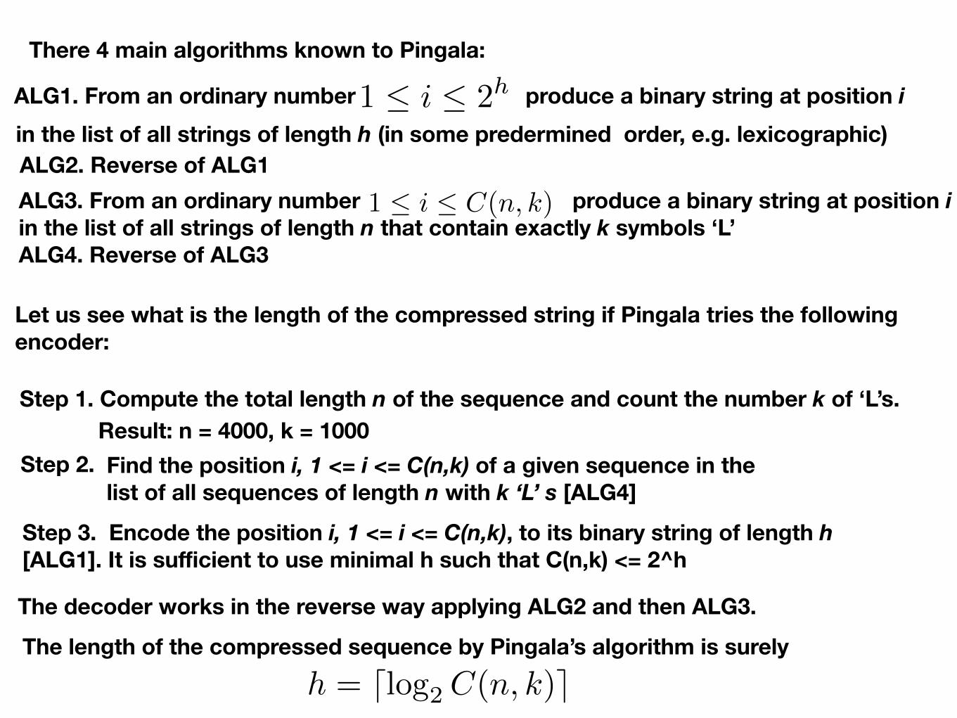
There 4 main algorithms known to Pingala:

ALG1. From an ordinary number produce a binary string at position iin the list of all strings of length h (in some predermined order, e.g. lexicographic)ALG2. Reverse of ALG1ALG3. From an ordinary number produce a binary string at position i in the list of all strings of length n that contain exactly k symbols ‘L’ ALG4. Reverse of ALG3

1 i C(n, k)

Let us see what is the length of the compressed string if Pingala tries the following encoder:

Step 1. Compute the total length n of the sequence and count the number k of ‘L’s.

Step 2. Result: n = 4000, k = 1000Find the position i, 1 <= i <= C(n,k) of a given sequence in the list of all sequences of length n with k ‘L’ s [ALG4]

Step 3. Encode the position i, 1 <= i <= C(n,k), to its binary string of length h [ALG1]. It is sufficient to use minimal h such that C(n,k) <= 2^h

1 i 2h

The decoder works in the reverse way applying ALG2 and then ALG3.

The length of the compressed sequence by Pingala’s algorithm is surelyh = dlog2 C(n, k)e

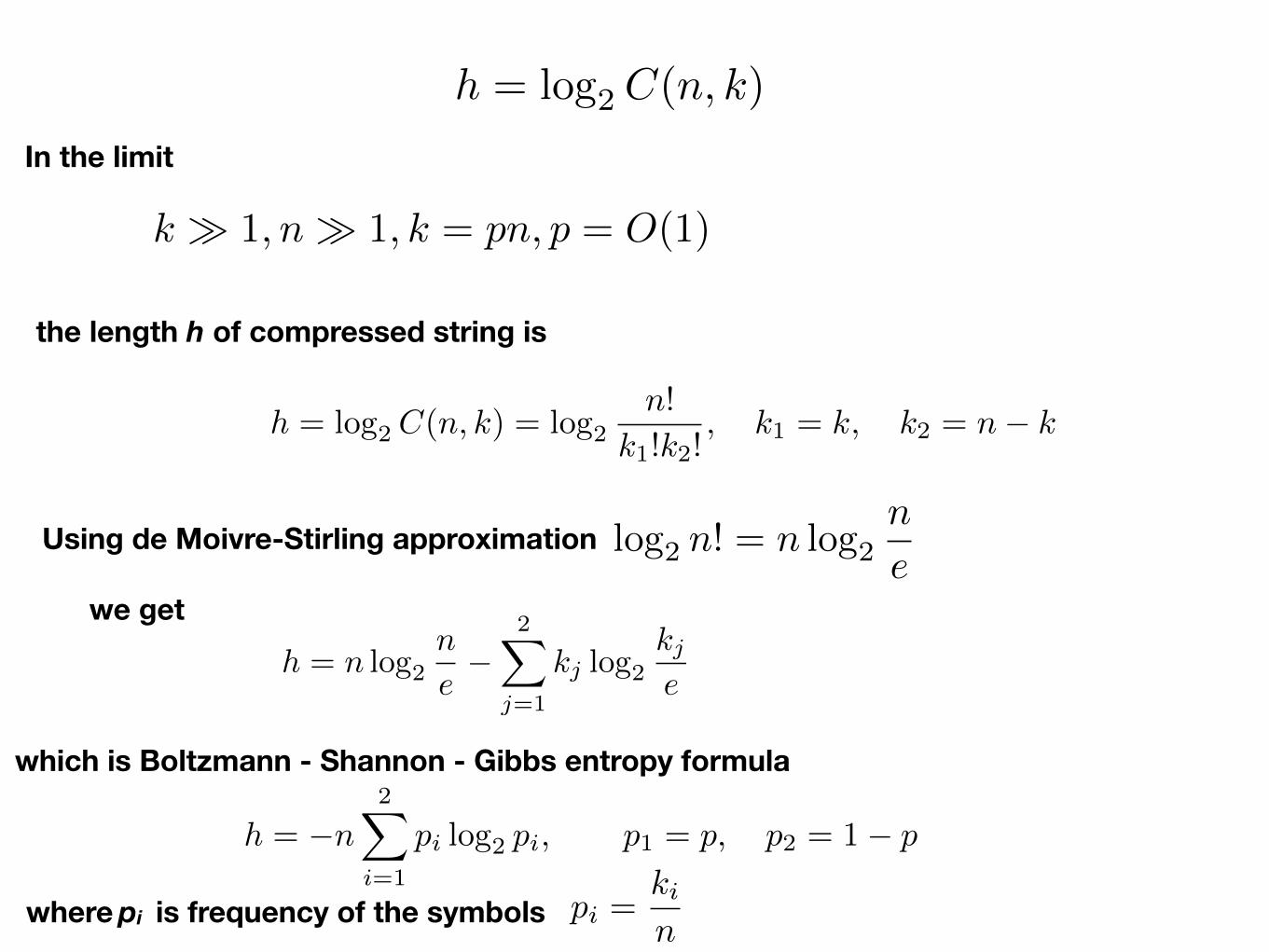
k � 1, n � 1, k = pn, p = O(1)

h = log2 C(n, k)

In the limit

the length h of compressed string is

Using de Moivre-Stirling approximation log2 n! = n log2n

ewe get

h = log2 C(n, k) = log2n!

k1!k2!, k1 = k, k2 = n� k

h = n log2n

e�

2X

j=1

kj log2kje

which is Boltzmann - Shannon - Gibbs entropy formula

h = �n2X

i=1

pi log2 pi, p1 = p, p2 = 1� p

where pi is frequency of the symbols pi =kin

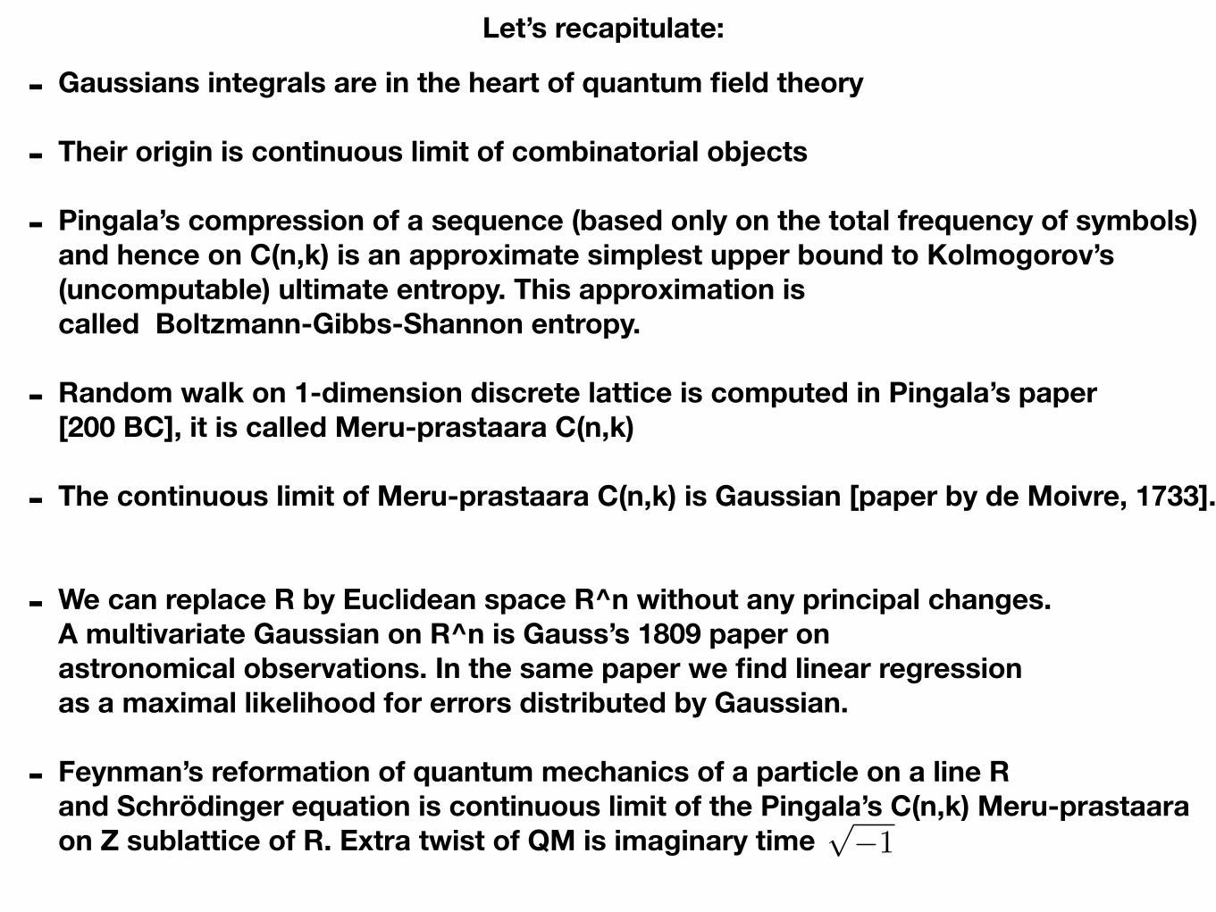
Let’s recapitulate:

- Gaussians integrals are in the heart of quantum field theory

- Their origin is continuous limit of combinatorial objects

- Pingala’s compression of a sequence (based only on the total frequency of symbols) and hence on C(n,k) is an approximate simplest upper bound to Kolmogorov’s (uncomputable) ultimate entropy. This approximation is called Boltzmann-Gibbs-Shannon entropy.

- Random walk on 1-dimension discrete lattice is computed in Pingala’s paper [200 BC], it is called Meru-prastaara C(n,k)

- The continuous limit of Meru-prastaara C(n,k) is Gaussian [paper by de Moivre, 1733].

- We can replace R by Euclidean space R^n without any principal changes. A multivariate Gaussian on R^n is Gauss’s 1809 paper on astronomical observations. In the same paper we find linear regression as a maximal likelihood for errors distributed by Gaussian.

- Feynman’s reformation of quantum mechanics of a particle on a line R and Schrödinger equation is continuous limit of the Pingala’s C(n,k) Meru-prastaaraon Z sublattice of R. Extra twist of QM is imaginary time

p�1

What is next?

The summary was essentially the state of the art circa 1810 about information geometry.

Except that imaginary time came later with quantum mechanics.

The essentially new ideas that appeared after 1810 and continued to the modern mathematics are:

- look on intrinsically non-flat spaces in geometry - look non-commutative structures in algebra

In geometry, in 1828 Gauss understood 2d surfaces as a 2-dimensional manifold, and in about 1850 Riemann proposed a version of non-flat n-dimensional spaces.

In algebra, in 1820-1830 Galois and Abel started the theory of groups in which multiplication operation was no more necessary commutative.

So what if we combine these new ideas of non-commutative multiplication and non-flat geometry with the random-walk process on the 1-dimensional line obtained by de Moivre from the Pingala’s combinatorics of binary sequences?

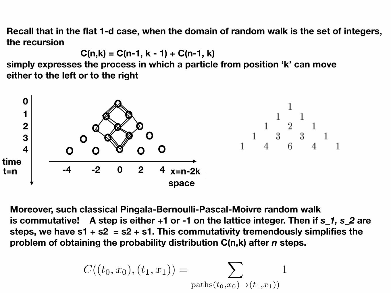
Moreover, such classical Pingala-Bernoulli-Pascal-Moivre random walk is commutative! A step is either +1 or -1 on the lattice integer. Then if s_1, s_2 are steps, we have s1 + s2 = s2 + s1. This commutativity tremendously simplifies the problem of obtaining the probability distribution C(n,k) after n steps.

Recall that in the flat 1-d case, when the domain of random walk is the set of integers, the recursion C(n,k) = C(n-1, k - 1) + C(n-1, k) simply expresses the process in which a particle from position ‘k’ can move either to the left or to the right

t=n 0 2 4-2-4

01234

time

spacex=n-2k

C((t0, x0), (t1, x1)) =X

paths(t0,x0)!(t1,x1))

1

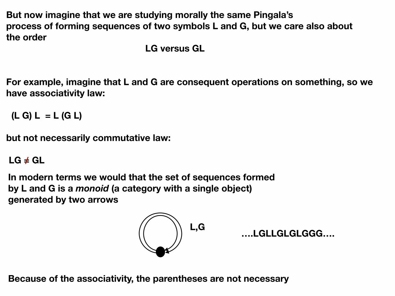
But now imagine that we are studying morally the same Pingala’s process of forming sequences of two symbols L and G, but we care also about the order LG versus GL

For example, imagine that L and G are consequent operations on something, so we have associativity law:

(L G) L = L (G L)

but not necessarily commutative law:

LG = GL

In modern terms we would that the set of sequences formed by L and G is a monoid (a category with a single object) generated by two arrows

/

L,G ….LGLLGLGLGGG….

Because of the associativity, the parentheses are not necessary

So, instead of Pingala’s (100-200 BC) random walk generated by L = -1 and G=+1 on the flat line where the composition operation is abelian, starting from 19th century we will consider random walks on curved spaces where the order of steps does matter!

A

B

path Φ

In physics this brought non-abelian gauge theory (Yang-Mills theory) and Einstein’s general relativity

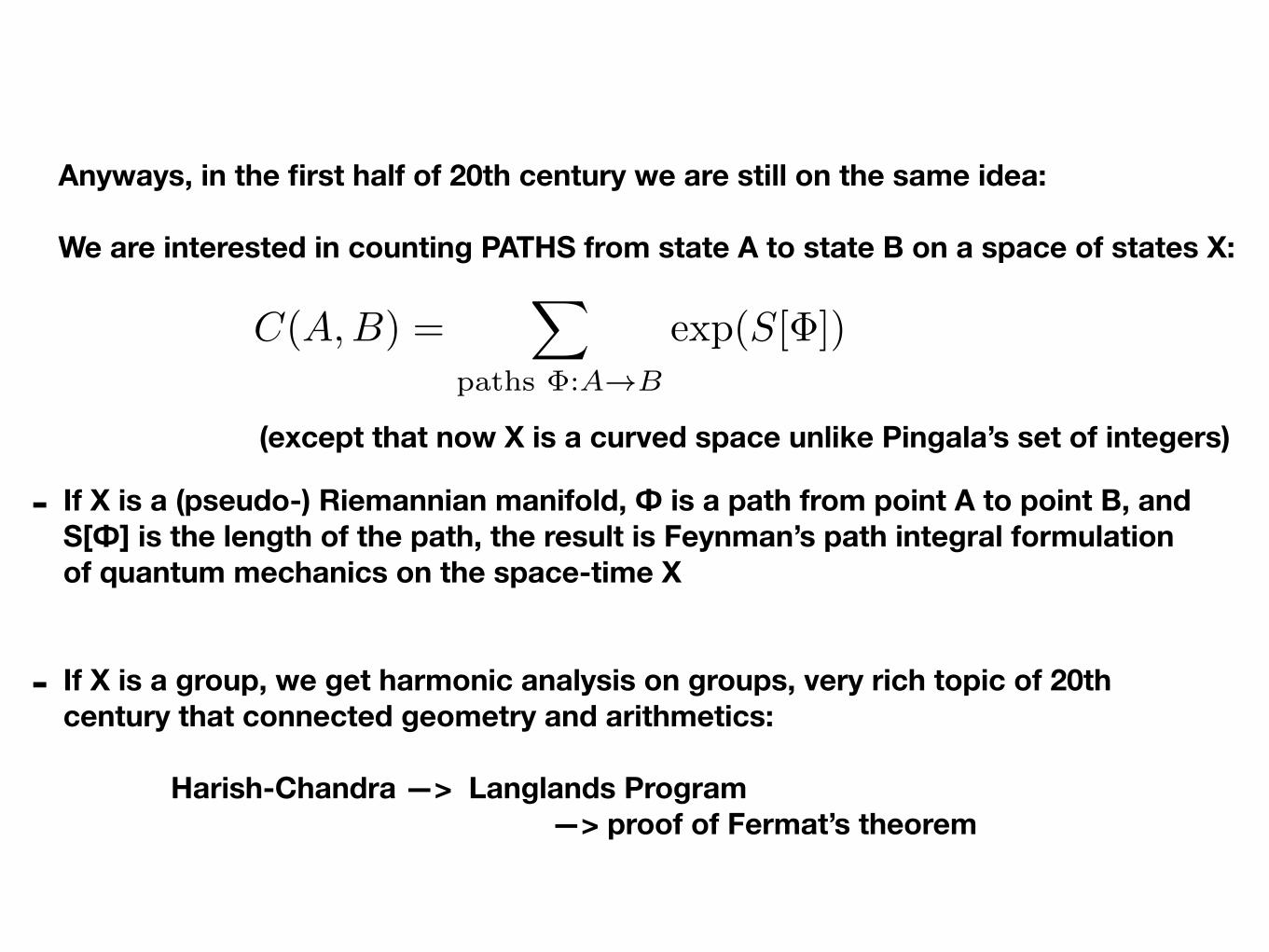
Anyways, in the first half of 20th century we are still on the same idea:

We are interested in counting PATHS from state A to state B on a space of states X:

C(A,B) =X

paths �:A!B

exp(S[�])

- If X is a (pseudo-) Riemannian manifold, Ф is a path from point A to point B, and S[Ф] is the length of the path, the result is Feynman’s path integral formulation of quantum mechanics on the space-time X

- If X is a group, we get harmonic analysis on groups, very rich topic of 20th century that connected geometry and arithmetics: Harish-Chandra —> Langlands Program —> proof of Fermat’s theorem

(except that now X is a curved space unlike Pingala’s set of integers)

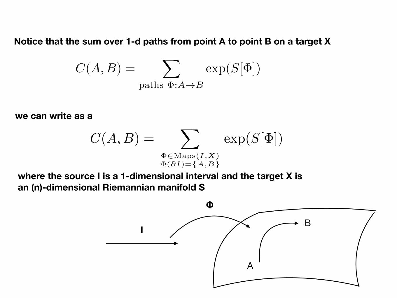
where the source I is a 1-dimensional interval and the target X is an (n)-dimensional Riemannian manifold S

Notice that the sum over 1-d paths from point A to point B on a target X

C(A,B) =X

paths �:A!B

exp(S[�])

we can write as a

I

A

B

Φ

C(A,B) =X

�2Maps(I,X)�(@I)={A,B}

exp(S[�])

So in the first half of 20th century the follow-ups on Pingala’s paper counted Maps(I,X)

where the source I is 1-dimensional, and the target X is a classical geometrical space (the dimension of X is not as important for complexity)

- quantum mechanics, harmonic analysis, stochastic processes, Markov chains, probabilistic automata……

What is next?

This gives

What gradually happened in the course of the second half of 20th century (and keeps going in the 21st) is the upgrade of the dimension of the source I

now we take the source I to be an n-dimensional manifold!

C(A,B) =X

�2Maps(I,X)�(@I)={A,B}

exp(S[�])

However, keeping the same idea

Remark: Maps(I,X) = XI

It is much more difficult to increase the dimension of the source I .if we discretize I and X to size N in every direction, then

|XI | = (NdX )NdI

= NdXNdI= exp(dXNdI logN)

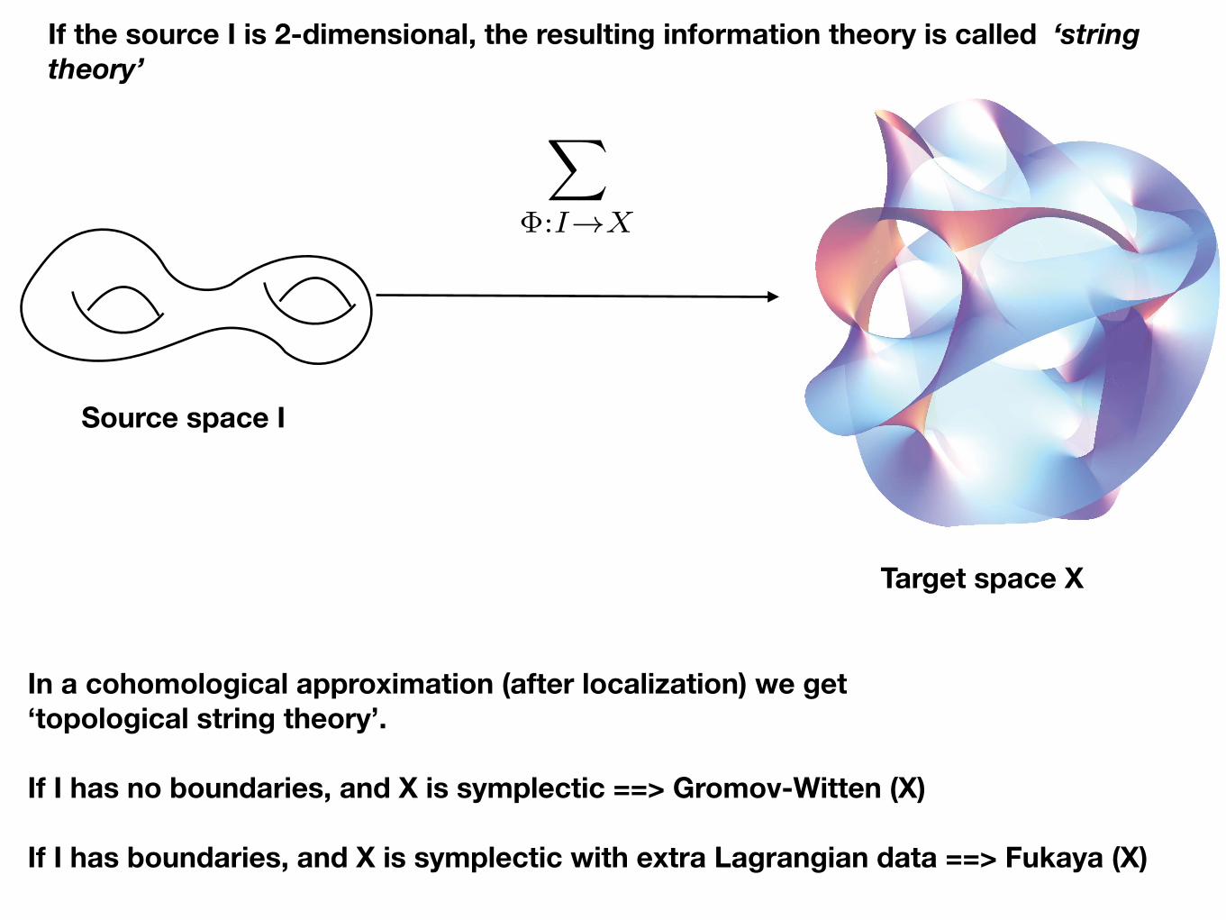
If the source I is 2-dimensional, the resulting information theory is called ‘string theory’

Source space I

Target space X

X

�:I!X

In a cohomological approximation (after localization) we get ‘topological string theory’.

If I has no boundaries, and X is symplectic ==> Gromov-Witten (X)

If I has boundaries, and X is symplectic with extra Lagrangian data ==> Fukaya (X)

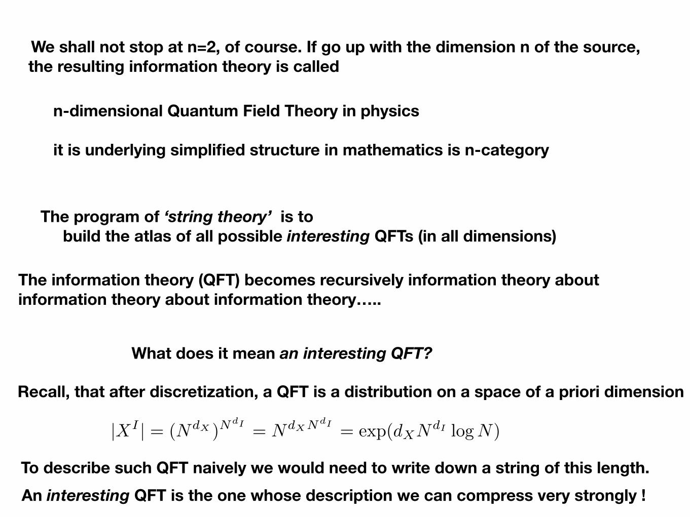
n-dimensional Quantum Field Theory in physics

it is underlying simplified structure in mathematics is n-category

We shall not stop at n=2, of course. If go up with the dimension n of the source, the resulting information theory is called

The program of ‘string theory’ is to build the atlas of all possible interesting QFTs (in all dimensions)

What does it mean an interesting QFT?

Recall, that after discretization, a QFT is a distribution on a space of a priori dimension

|XI | = (NdX )NdI

= NdXNdI= exp(dXNdI logN)

To describe such QFT naively we would need to write down a string of this length.An interesting QFT is the one whose description we can compress very strongly !

The information theory (QFT) becomes recursively information theory about information theory about information theory…..

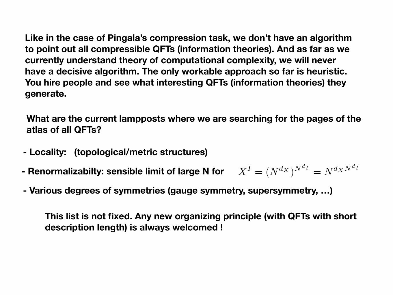
Like in the case of Pingala’s compression task, we don’t have an algorithm to point out all compressible QFTs (information theories). And as far as we currently understand theory of computational complexity, we will never have a decisive algorithm. The only workable approach so far is heuristic. You hire people and see what interesting QFTs (information theories) they generate.

What are the current lampposts where we are searching for the pages of the atlas of all QFTs?

- Renormalizabilty: sensible limit of large N for

- Locality: (topological/metric structures)

- Various degrees of symmetries (gauge symmetry, supersymmetry, …)

This list is not fixed. Any new organizing principle (with QFTs with short description length) is always welcomed !

XI = (NdX )NdI

= NdXNdI

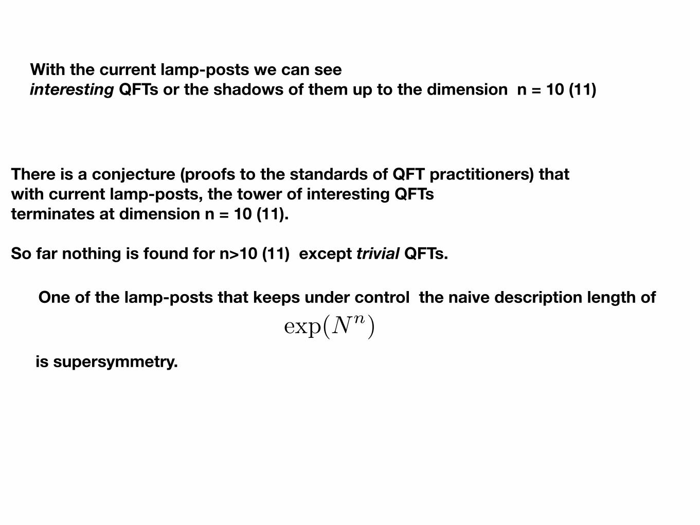
With the current lamp-posts we can see interesting QFTs or the shadows of them up to the dimension n = 10 (11)

There is a conjecture (proofs to the standards of QFT practitioners) that with current lamp-posts, the tower of interesting QFTs terminates at dimension n = 10 (11).

So far nothing is found for n>10 (11) except trivial QFTs.

One of the lamp-posts that keeps under control the naive description length of

is supersymmetry.

exp(Nn)

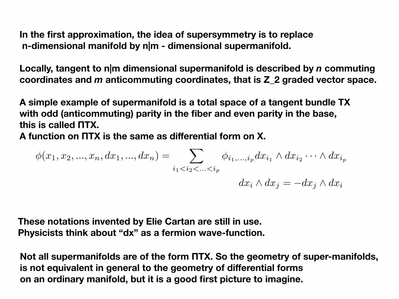
In the first approximation, the idea of supersymmetry is to replace n-dimensional manifold by n|m - dimensional supermanifold.

Locally, tangent to n|m dimensional supermanifold is described by n commuting coordinates and m anticommuting coordinates, that is Z_2 graded vector space.

A simple example of supermanifold is a total space of a tangent bundle TX with odd (anticommuting) parity in the fiber and even parity in the base, this is called ПTX. A function on ПTX is the same as differential form on X.

These notations invented by Elie Cartan are still in use. Physicists think about “dx” as a fermion wave-function.

�(x1, x2, ..., xn, dx1, ..., dxn) =X

i1<i2<...<ip

�i1,...,ipdxi1 ^ dxi2 · · · ^ dxip

dxi ^ dxj = �dxj ^ dxi

Not all supermanifolds are of the form ПТX. So the geometry of super-manifolds, is not equivalent in general to the geometry of differential forms on an ordinary manifold, but it is a good first picture to imagine.

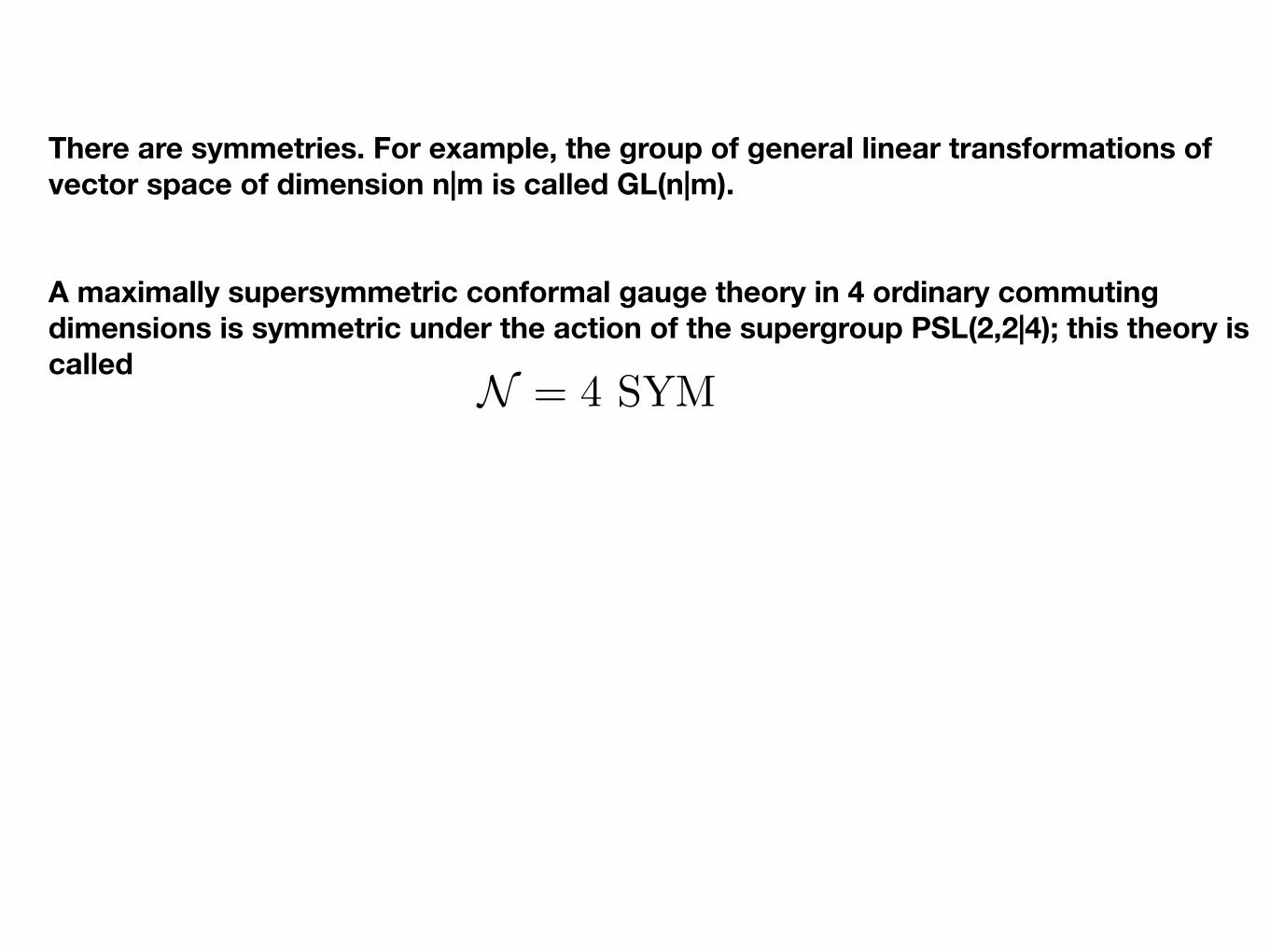
There are symmetries. For example, the group of general linear transformations of vector space of dimension n|m is called GL(n|m).

A maximally supersymmetric conformal gauge theory in 4 ordinary commuting dimensions is symmetric under the action of the supergroup PSL(2,2|4); this theory is called

N = 4 SYM

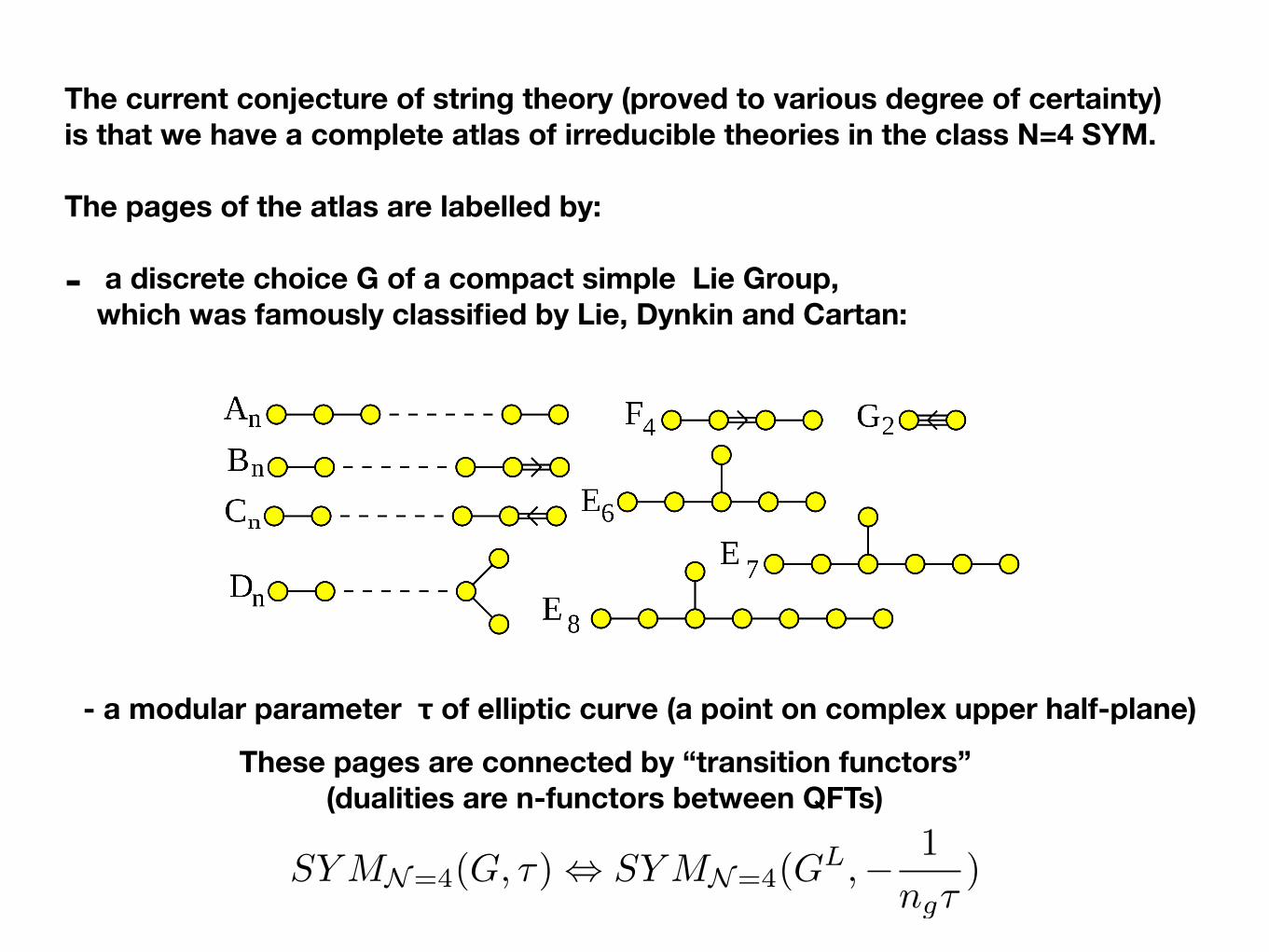
The current conjecture of string theory (proved to various degree of certainty) is that we have a complete atlas of irreducible theories in the class N=4 SYM.

The pages of the atlas are labelled by:

- a discrete choice G of a compact simple Lie Group, which was famously classified by Lie, Dynkin and Cartan:

- a modular parameter τ of elliptic curve (a point on complex upper half-plane)

These pages are connected by “transition functors” (dualities are n-functors between QFTs)

SYMN=4(G, ⌧) , SYMN=4(GL,� 1

ng⌧)

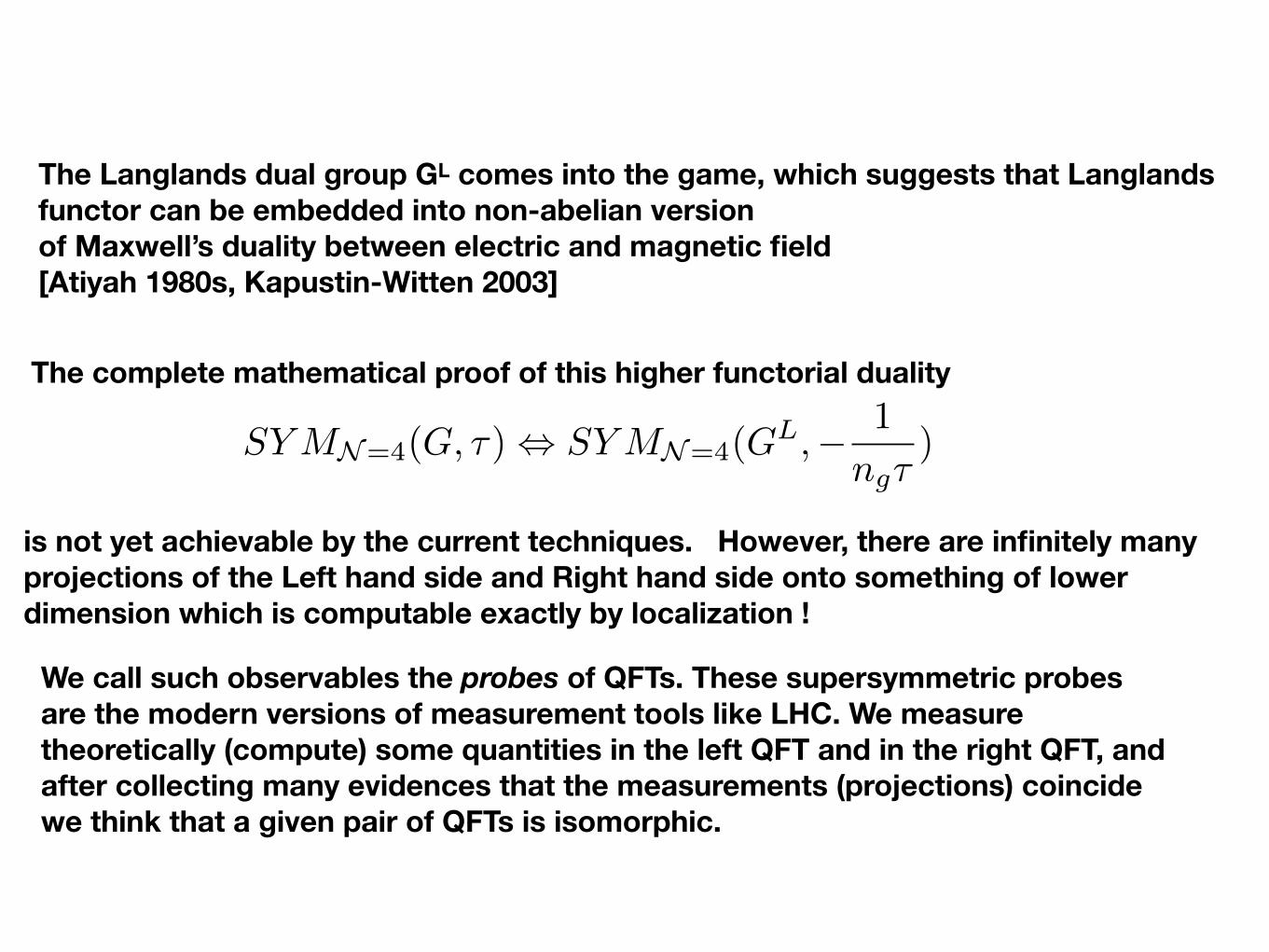
The Langlands dual group GL comes into the game, which suggests that Langlands functor can be embedded into non-abelian version of Maxwell’s duality between electric and magnetic field [Atiyah 1980s, Kapustin-Witten 2003]

SYMN=4(G, ⌧) , SYMN=4(GL,� 1

ng⌧)

The complete mathematical proof of this higher functorial duality

is not yet achievable by the current techniques. However, there are infinitely many projections of the Left hand side and Right hand side onto something of lower dimension which is computable exactly by localization !

We call such observables the probes of QFTs. These supersymmetric probes are the modern versions of measurement tools like LHC. We measure theoretically (compute) some quantities in the left QFT and in the right QFT, and after collecting many evidences that the measurements (projections) coincide we think that a given pair of QFTs is isomorphic.

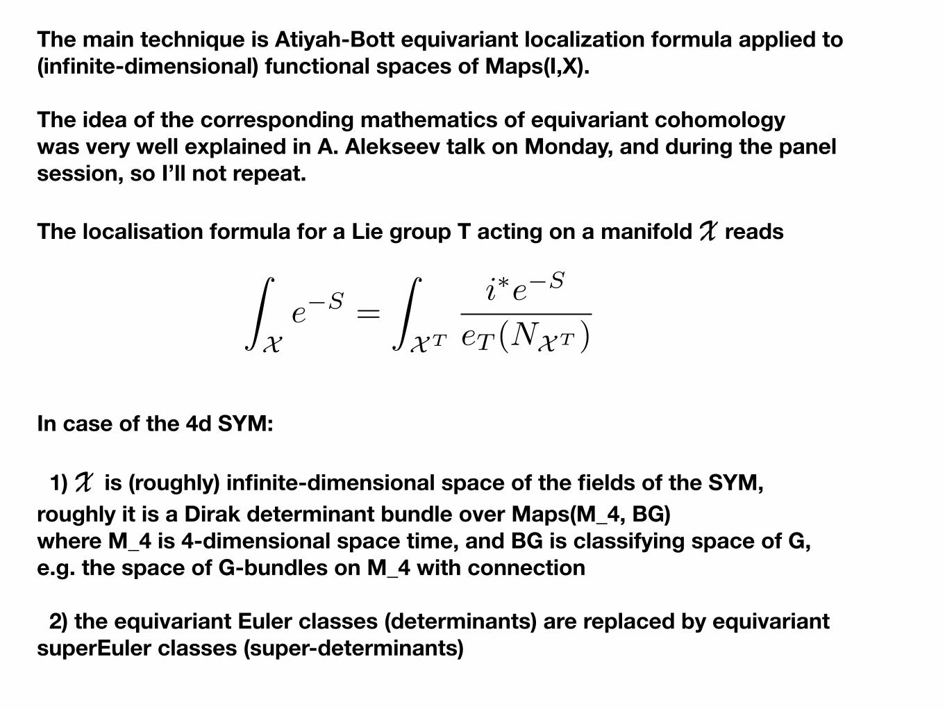
The main technique is Atiyah-Bott equivariant localization formula applied to (infinite-dimensional) functional spaces of Maps(I,X).

The idea of the corresponding mathematics of equivariant cohomology was very well explained in A. Alekseev talk on Monday, and during the panel session, so I’ll not repeat.

The localisation formula for a Lie group T acting on a manifold X reads

In case of the 4d SYM:

1) X is (roughly) infinite-dimensional space of the fields of the SYM, roughly it is a Dirak determinant bundle over Maps(M_4, BG) where M_4 is 4-dimensional space time, and BG is classifying space of G, e.g. the space of G-bundles on M_4 with connection

2) the equivariant Euler classes (determinants) are replaced by equivariant superEuler classes (super-determinants)

Z

Xe�S =

Z

XT

i⇤e�S

eT (NXT )

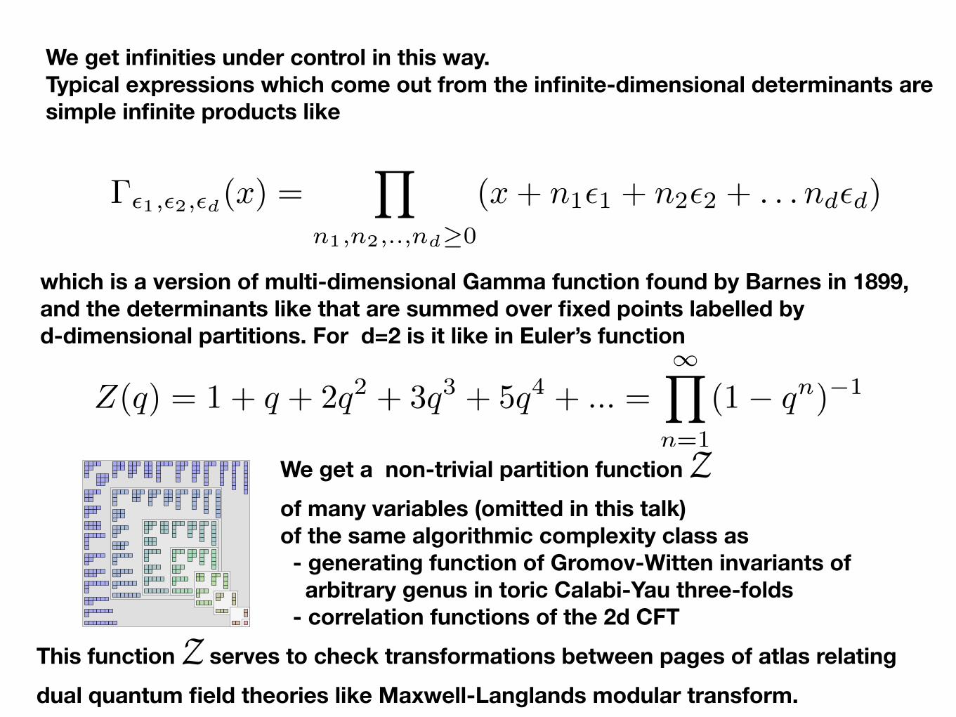
We get infinities under control in this way. Typical expressions which come out from the infinite-dimensional determinants are simple infinite products like

�✏1,✏2,✏d(x) =Y

n1,n2,..,nd�0

(x+ n1✏1 + n2✏2 + . . . nd✏d)

which is a version of multi-dimensional Gamma function found by Barnes in 1899, and the determinants like that are summed over fixed points labelled by d-dimensional partitions. For d=2 is it like in Euler’s function

Z(q) = 1 + q + 2q2 + 3q3 + 5q4 + ... =1Y

n=1

(1� qn)�1

6/23/2016 Ferrer_partitioning_diagrams.svg

file:///Users/pestun/Dropbox/travel/2016-06-Brazil/Ferrer_partitioning_diagrams.svg 1/1

We get a non-trivial partition function Zof many variables (omitted in this talk) of the same algorithmic complexity class as - generating function of Gromov-Witten invariants of arbitrary genus in toric Calabi-Yau three-folds - correlation functions of the 2d CFT

This function Z serves to check transformations between pages of atlas relating dual quantum field theories like Maxwell-Langlands modular transform.

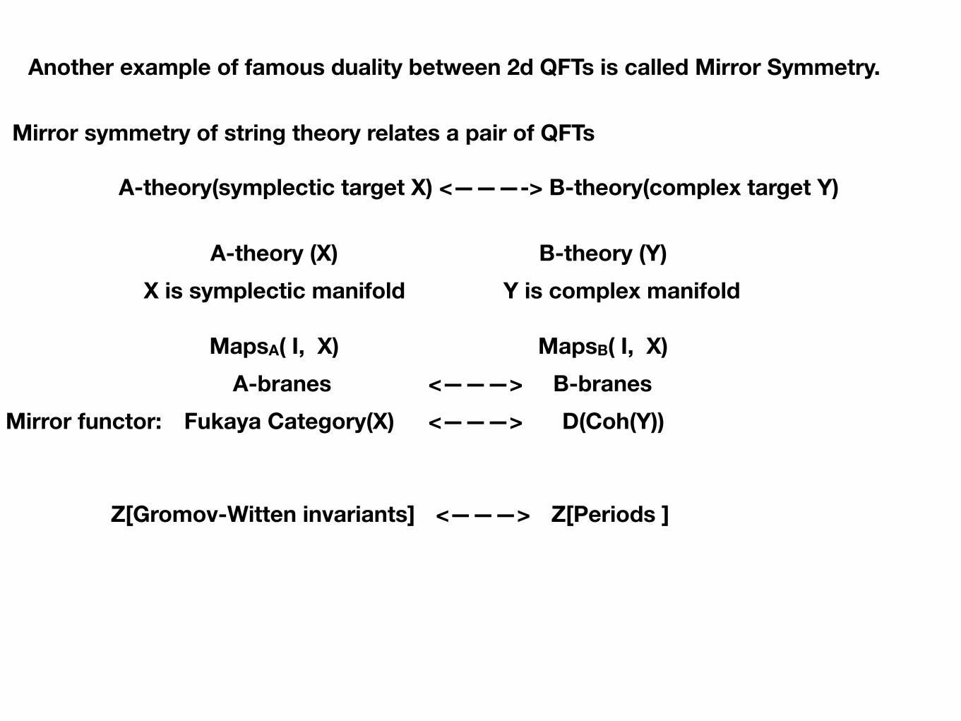
Another example of famous duality between 2d QFTs is called Mirror Symmetry.

Mirror symmetry of string theory relates a pair of QFTs

A-theory(symplectic target X) <———-> B-theory(complex target Y)

A-theory (X) B-theory (Y)

MapsA( I, X) MapsB( I, X)

X is symplectic manifold Y is complex manifold

Fukaya Category(X) D(Coh(Y)) <———>Mirror functor:

Z[Gromov-Witten invariants] Z[Periods ]

A-branes B-branes

<———>

<———>

60 P. Candelas et at / Calabi-Yau manifolds

TABLE 4 The numbers of rational curves of degree k for 1 ~< k ~< 10

k nk

1 2875 2 609250 3 3172 06375 4 24 2467530000 5 22930 58888 87625 6 248 24974 21180 22000 7 2 95091 05057 08456 59250 8 3756 3216093747 66035 50000 9 50 38405 10416 98524 36451 06250

I0 70428 81649 78454 68611 34882 49750

number of conics [28] (rational curves of degree two). Clemens has shown [30] that n~ ~: 0 for infinitely many k and has conjectured that n k ~: 0 for all k, but it seems that the direct calculation of these numbers becomes difficult beyond k = 2 (see also ref. [28]). It is however straightforward to develop the series (5.12) to more terms and to find the n~ by comparison with (5.13). We present the first few n k in table 4. These numbers provide compelling evidence that our assumption about the form of the prefactor is in fact correct. The evidence is not so much that we obtain in this way the correct values for n~ and n 2, but rather that the coefficients in eq. (5.12) have remarkable divisibility properties. For example asserting that the second coefficient 4,876,875 is of the form 23n2 + n I requires that the result of subtracting n~ from the coefficient yields an integer that is divisible by 2 3.

Similarly, the result of subtracting n~ from the third coefficient must yield an integer divisible by 3 3. These conditions become increasingly intricate for large k. It is therefore remarkable that the n k calculated in this way turn out to be integers.

The values for the nk shown in the table are particular to P4(5), however we can abstract from eq. (5.13) a form for the mirror map which we conjecture to be of general validity,

e2rri.2,'[w] = . ~ 3 (5 .14) 7~v ~e'w + .2'~t¢~] 1 - e 2~'i-2'[w1

where we regard the complex structure of 7 f as being parametrized by the complex K~ihler form w = B + / J of ~#, and

Nuclear Physics B359 (1991) 21-74 North-Holland

A PAIR OF CALABI-YAU MANIFOLDS AS AN EXACTLY SOLUBLE SUPERCONFORMAL THEORY*

Philip CANDELAS l, Xenia C. DE LA OSSA l-**, Paul S. G R E E N 2 and Linda PARKES t

I Theory Group, Department of Physics, The Unicersity of Texas, Austin, IX 78746, USA 2Depanmo~t of Mathematics, University of Maryland, College Park, MD 20742, USA

Received 31 October 1990 (Revised 1 February 1991)

We compute the prepotentials and the geometry of the moduli spaces for a Calabi-Yau manifold and its mirror. In this way we obtain all the sigma model corrections to the Yukawa couplings and moduli space metric for the original manifold. The moduli space is found to be subject to the action of a modular group which, among other operations, exchanges large and small values of the radius, though the action on the radius is not as simple as R ~ 1 /R. It is a - ~ shown that the quantum corrections to the coupling decompose into a sum over instanton contributions and moreover that this sum converges. In particular there are no "'sub-instanton'" corrections. This sum over instantons points to a deep connection between the modular group and the rational curves of the Calabi-Yau manifold. The burden of the present work is that a mirror pair of Calabi-Yau manifolds is an exactly soluble superconformai theory, at least as far as the massless sector is concerned. Mirror pairs are also more general than exactly soluble models that have hitherto been discussed since we solve the theory for all points of the moduli space.

1. Introduction

The discovery of mirror symmetry [1-3] among pairs of Calabi-Yau manifolds goes a long way towards resolving a long standing puzzle. A Calabi-Yau mani- fold .,~/possesses a certain number of parameters. These are parameters associ- ated with the structure of ¢~' as a complex manifold and parameters corresponding to the deformations of the K/ihler metric of f / . These parameters, which are related to the cohomology of /~ ' , give rise to families and antifamilies of particles in the effective low-ener~ theory that results from compactification of the string. The parameters corresponding to deformations of the complex structure are related to the cohomology group H 21 of (2, 1)-forms while the parameters corre-

* Supported in part by the Robert A. Welch Foundation and NSF grants PHY-880637 and PHY- 8605978.

** Present address: Escuela de Fisica, Universidad de Costa Rica, San Pedro de Monies de Oca, Costa Rica.

0550-3213/91/$03.50 © 1991 - Elsevier Science Publishers B.V. (North-Holland)

https://arxiv.org/abs/alg-geom/9301006v2

arX

iv:a

lg-g

eom

/930

1006

v2 1

Feb

199

3

OSU-M-92-3

Rational curves on Calabi-Yau manifolds: verifyingpredictions of Mirror Symmetry

Sheldon KatzDepartment of MathematicsOklahoma State University

Stillwater, OK 74078email: katz@math.okstate.edu

Recently, mirror symmetry, a phenomenon in superstring theory, has beenused to give tentative calculations of several numbers in algebraic geometry 1.This yields predictions for the number of rational curves of any degree d ongeneral Calabi-Yau hypersurfaces in P4 [2], P(2, 14), P(4, 14), and P(5, 2, 13)[4, 9, 11]. The techniques used in the calculation rely on manipulationsof path integrals which have not yet been put on a rigorous mathematicalfooting. On the other hand, there is currently no prospect of calculatingmost of these numbers by algebraic geometry.

Until this point, three of these numbers have been verified, all for thequintic hypersurface in P4: the number of lines (2875) was known classically,the number of conics (609250) was calculated in [7], and the number oftwisted cubics (317206375) was found recently by Ellingsrud and Strømme[3].

Even more recently [6], higher dimensional mirror symmetry has beenused to predict the number of rational curves on Calabi-Yau hypersurfacesin higher dimensional projective spaces which meet 3 linear subspaces ofcertain dimensions. Again, there is no known way to calculate these usingalgebraic geometry.

The purpose of this paper is to verify some of these numbers in lowdegree, giving more evidence for the validity of mirror symmetry. In §1,the number of weighted lines in a weighted sextic in P(2, 14) is calculated,

1See the papers in [14] for general background on mirror symmetry.

1

Number of rational curves of degree k in quintic Calabi-Yau (degree 5) three-dimensional hypersurface in P4

string theory localization 1990 “conventional” algebraic geometry 1993

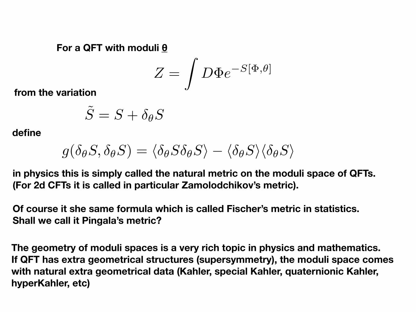
S = S + �✓S

Z =

ZD�e�S[�,✓]

For a QFT with moduli θ

from the variation

g(�✓S, �✓S) = h�✓S�✓Si � h�✓Sih�✓Siin physics this is simply called the natural metric on the moduli space of QFTs. (For 2d CFTs it is called in particular Zamolodchikov’s metric).

Of course it she same formula which is called Fischer’s metric in statistics. Shall we call it Pingala’s metric?

The geometry of moduli spaces is a very rich topic in physics and mathematics. If QFT has extra geometrical structures (supersymmetry), the moduli space comes with natural extra geometrical data (Kahler, special Kahler, quaternionic Kahler, hyperKahler, etc)

define

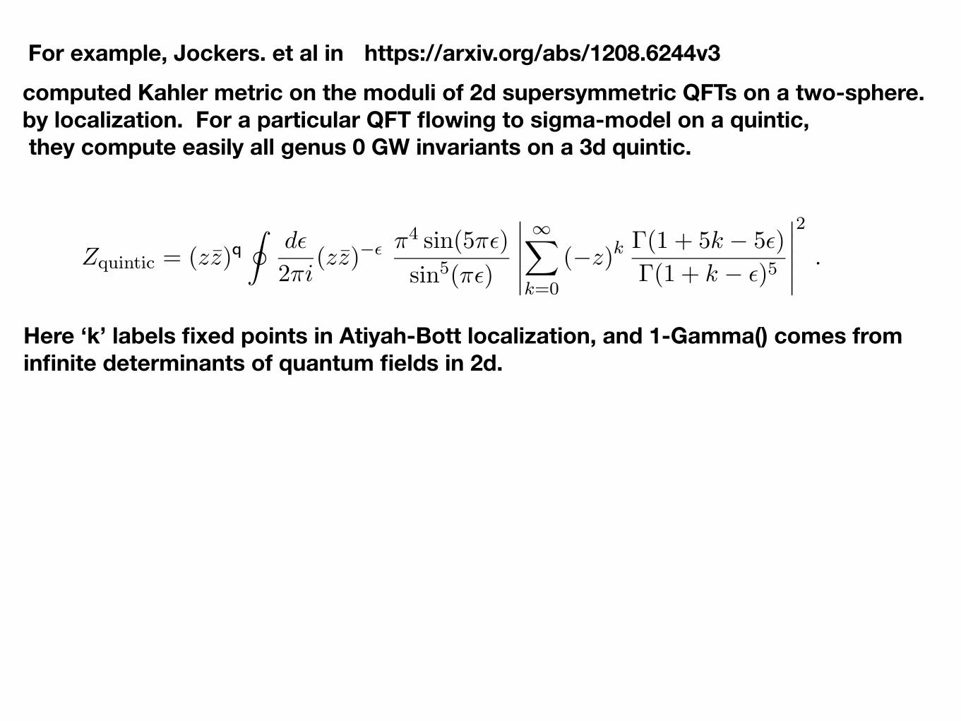
https://arxiv.org/abs/1208.6244v3For example, Jockers. et al in computed Kahler metric on the moduli of 2d supersymmetric QFTs on a two-sphere. by localization. For a particular QFT flowing to sigma-model on a quintic, they compute easily all genus 0 GW invariants on a 3d quintic.

gation does not act on ϵ, and where z := exp(−2πr + iθ). For the quintic (n = 5), we have

Zquintic = (zz)q∮

dϵ

2πi(zz)−ϵ π4 sin(5πϵ)

sin5(πϵ)

∣∣∣∣∣

∞∑

k=0

(−z)kΓ(1 + 5k − 5ϵ)

Γ(1 + k − ϵ)5

∣∣∣∣∣

2

. (4.6)

Having required 0 < q < 15 , notice that the remaining dependence on q is only through an overall

multiplicative factor that can be removed by a Kahler transformation. In what follows, we will

disregard the pre-factor (zz)q by taking q → 15−

(this is the natural choice of R-charge here

since this model has a Landau-Ginzburg phase where P obtains a vev, but for models without

Landau-Ginzburg phases it is less clear from the UV theory how one should choose q).

We now demonstrate that the Gromov–Witten invariants, as determined by the procedure of

Section 3.3, agree with those computed in [6]. First we extract the coefficient of ζ(3) in (4.6),

which determines the Kahler transformation X0(z) to be performed. After performing the Kahler

transformation, the Kahler potential becomes

e−K ′

= −1

8π3

Zquintic

X0(z)X0(z), (4.7)

where

X0(z) =∞∑

k=0

Γ(1 + 5k)

Γ(1 + k)5(−z)k . (4.8)

It is interesting to observe that X0(z) is precisely the “fundamental period” of the quintic as

determined by mirror symmetry (z is rescaled by a factor of −55 relative to the formulas in [6]).

This suggests that our methods are closely related to toric mirror symmetry [63,64], in which the

periods are known [65] to be generalized hypergeometric functions [66].

Next, we determine the mirror map through the coefficient of the log2 z term, which yields

t = t(0) +1

2πi

(log z − 770 z + 717 825 z2 + . . .

). (4.9)

Inverting the mirror map, we find that the leading instanton correction is exactly −2875e−2πit(0) ,

fixing the undetermined constant t(0) ∈ [0, 1) to be t(0) =12 . With this choice, the integral genus

zero Gromov–Witten invariants are

2 875 , 609 250 , 317 206 375 , 242 467 530 000 , . . . , (4.10)

and agree with the numbers in the literature [6].

4.2 Rødland’s Pfaffian Calabi–Yau threefold

In this section, we analyze the partition function of a Calabi–Yau subvariety of P6 defined by

the rank 4 locus of a 7 × 7 antisymmetric matrix whose entries are linear in the homogeneous

coordinates of P6. Rødland conjectured that this Calabi–Yau threefold is in the same Kahler

moduli space as a complete intersection of seven hyperplanes in the Grassmannian G(2, 7) [61],

13

Here ‘k’ labels fixed points in Atiyah-Bott localization, and 1-Gamma() comes from infinite determinants of quantum fields in 2d.

63

Vasily Pestun, Maxim Zabzine, Francesco Benini, Tudor Dimofte,

Thomas T. Dumitrescu, Kazuo Hosomichi, Seok Kim,

Kimyeong Lee, Bruno Le Floch, Marcos Marino, Joseph A. Minahan, David R. Morrison, Sara Pasquetti,

Jian Qiu, Leonardo Rastelli, Shlomo S. Razamat, Silvu S. Pufu,

Yuji Tachikawa, Brian Willett, Konstantin Zarembo

Localization techniques in quantum field theories

review collection arXiv:1608.02952

For all fancy details of other localization use in QFT see 700 pages review :

to be continued…

Thank you all