Localized Algorithm for Precise BoundaryDetection in 3D Wireless Networks

Hongyu Zhou, Su Xia, Miao Jin, and Hongyi WuThe Center for Advanced Computer Studies

University of Louisiana at Lafayette

Lafayette, LA, USA

E-mail: {hxz6029,sxx1110,mjin,wu}@cacs.louisiana.edu

Abstract—This research focuses on distributed and localizedalgorithms for precise boundary detection in 3D wirelessnetworks. Our objectives are in two folds. First, we aim toidentify the nodes on the boundaries of a 3D network, whichserve as a key attribute that characterizes the network, especiallyin such geographic exploration tasks as terrain and underwaterreconnaissance. Second, we construct locally planarized 2-manifold surfaces for inner and outer boundaries, in order toenable available graph theory tools to be applied on 3D surfaces,such as embedding, localization, partition, and greedy routingamong many others. To achieve the first objective, we proposea Unit Ball Fitting (UBF) algorithm that discovers a set ofpotential boundary nodes, followed by a refinement algorithm,named Isolated Fragment Filtering (IFF), which removesisolated nodes that are misinterpreted as boundary nodes byUBF. Based on the identified boundary nodes, we developan algorithm that constructs a locally planarized triangularmesh surface for each 3D boundary. Our proposed scheme islocalized, requiring information within one-hop neighborhoodonly. Our simulation results demonstrate that the proposedalgorithms can effectively identify boundary nodes and surfaces,even under high measurement errors. As far as we know, this isthe first work for discovering boundary nodes and constructingboundary surfaces in 3D wireless networks.

Index Terms—3D; boundary detection; triangulation; wirelesssensor networks.

I. INTRODUCTION

Many wireless networks exhibit substantial randomness,due to the lack of precise nodal deployment and the non-deterministic failures and channel dynamics. Therefore, the fi-nal formation of a wireless network heavily depends on its un-derlying environment. Consequently, there is a primary interestto discover the unknown geometry and topology of a wirelessnetwork formation (or a subnetwork formation), which providesalient information for understanding its environment and forefficient operation of the network itself. In particular, boundaryis one of the key attributes that characterize the network intwo or three-dimensional space, especially in such geographicexploration tasks as terrain and underwater reconnaissance.

A. Related Work

The quest for efficient boundary detection in wireless net-works has led to two research thrusts outlined below:

Detection of Event Boundary

The investigation on boundary detection started from theestimation and localization of events in sensor networks. Thespatially distributed sensors usually report different measure-ments in respond to an event. For example, upon a fire,the sensors located in the fire are likely destroyed (and thusresulting a void area of failed nodes), while the sensors close tothe fire region measure higher temperature and smoke densitythan the faraway sensors do. Boundary detection is to delineatethe regions of distinct behavior in a sensor network [1].

Achieving accurate detection of event boundary is chal-lenging, because the sampling density is limited, the sensorreadings are noisy, the delivery of sensor data is unreliable,and the computation power of individual sensors is extremelylow [1], [2]. To this end, a series of studies have been carriedout to explore efficient information processing and modelingtechniques to analyze sensor data, in order to estimate theboundary of events [1]–[5].

Due to inevitable errors in raw sensor data, these approachesdo not yield precise boundary. Instead, they aim at a closeenough estimation that correctly identifies the events frontier,based on either global or local data collected from a set ofsensors.

Detection of Network Boundary

Besides the researches discussed above that are mainly fromthe data processing perspective, interests are also developedto precisely locate the boundary of the network based ongeometric or topology information of a wireless network.Noise in sensor data is no longer a concern here, becausesuch boundary detection is not based on sensor measurement.However, new challenges arise due to the required accuracy ofthe identified boundary, especially in networks with complexinner boundary (i.e., “holes”) or in high dimensional space.

Most proposed network boundary detection algorithms arebased on 2D graphic tools. For example, Voronoi diagramsare employed in [6], [7] to discover coverage holes in sensornetworks. Delaunay triangulation is adopted in [8] to iden-tify communication voids. In contrast to [6]–[8] that exploitsensor positions, two distributed algorithms are proposed in[9] by utilizing distance and/or angle information betweennodes to discover coverage boundary. In [10], an algebraictopological invariant called homology is computed to detect

(a) A 3D Network. (b) Boundary nodes. (c) Landmarks.

1074

1809

622

1138

69

1728

1547

649

79

854

1286

1862

861

1259

1127

348

965

658

1269

529

1942

1254

1614

505

1480

1921

907

2033

455

1833

24

72

6

1696

1951

1087

37

20041774

522

632

1085

1710

1695

1623

1666

764

577

1386

570

(d) CDG.

1074

1809

622

1138

69

1728

1547

649

79

854

1286

1862

861

1259

1127

348

965

658

1269

529

1942

1254

1614

505

1480

1921

907

2033

455

1833

24

72

6

1696

1951

1087

37

20041774

522

632

1085

1710

1695

1623

1666

764

577

1386

570

(e) CDM. (f) Triangular mesh.

0

500

1000

1500

2000

2500

0% 10% 20% 30% 40% 50% 60% 70% 80% 90% 100%

Num

ber o

f Bou

ndar

y N

odes

Distances Measurement Error

FoundCorrect

MistakenMissing

(g) Algorithm efficiency.

0%

20%

40%

60%

80%

100%

0% 10% 20% 30% 40% 50% 60% 70% 80% 90% 100%

Dis

tribu

tion

of M

ista

ken

Boun

dary

Nod

es

Distances Measurement Error

1 hop2 hop3 hop

(h) Mistaken distribution.

0%

20%

40%

60%

80%

100%

0% 10% 20% 30% 40% 50% 60% 70% 80% 90% 100%

Dis

tribu

tion

of M

issi

ng B

ound

ary

Nod

es

Distances Measurement Error

1 hop2 hop3 hop

(i) Missing distribution.

(j) 20% distance measurement errors. (k) 30% distance measurement errors. (l) 40% distance measurement errors.

Fig. 1. Illustration of the proposed boundary detection algorithm (based on a 3D wireless network of 4210 nodes with an average nodal degree of 18.8).

holes. The algorithm is generally applicable to networks in anydimensional space. However, it is a centralized approach andthere is significant challenge to decentralize its computation[10]. In [11], the isosets (each of which consists of nodeswith the same hop distance to a beacon node) are identified.The disconnection in an isoset indicates the boundary nodesof holes. Multiple beacons can be employed to locate theboundary nodes at different directions of a hole. This approachdoes not guarantee to discover the complete boundary of every

hole. Higher accuracy can be achieved if more beacons areemployed or when the network is denser. [12] introduces a de-terministic algorithm for boundary detection. It searches for aspecial subgraph structure, called m-flower, which is boundedby a circle. Once a m-flower is identified, the algorithm cansubsequently find the boundary nodes through a number ofiterations of augmentation of the circle. But not every graphhas an m-flower structure. Therefore, the algorithm may failespecially when the nodal density is low. In [13], a shortest

path tree is built to find the shortest circle, which is thenrefined to discover the tight boundaries of the inner holes.

All of the network boundary detection approaches discussedabove are developed for networks in 2D space. Except [10]which is centralized, none of them can be readily appliedto 3D networks since higher dimension space introducessignificant complexity in searching for boundaries and manytopological and geometrical tools cannot be extended from2D to 3D. In addition, while boundary extraction has beenextensively studied in 3D imaging, the algorithms developedtherein always assume grid-like 3D pixels as inputs, whichare in sharp contrast to network settings where nodes are ran-domly distributed, and thus are not applicable in 3D wirelessnetworks.

B. Our Contribution

There are increasing interests in 3D wireless networks,with several areas such as routing [14]–[19], localization [20],nodal placement [21], [22], physical layer investigation [23]and applications [23], [24], being explored recently. Thisresearch aims to develop distributed and localized algorithmsfor precise boundary detection in 3D wireless networks. Ourobjectives are in two folds:

(1) First, we aim to identify the nodes on the boundaries ofa 3D network (see Fig. 1(b) for example).

(2) Second, we construct locally planarized 2-manifold sur-faces for inner and outer boundaries (as shown inFig. 1(f)).

To achieve the first objective, we propose a Unit Ball Fitting(UBF) algorithm that discovers a set of potential boundarynodes, followed by a refinement algorithm, named IsolatedFragment Filtering (IFF), which removes isolated nodes thatare misinterpreted as boundary nodes by UBF. Our proposedscheme is localized, requiring information within one-hopneighborhood only.

The boundary nodes are discrete. They serve as samplepoints that depict the network boundaries. However, many ap-plications desire not only such discrete points, but also closedboundary surfaces, especially locally planarized 2-manifold inorder to apply available graph theory tools on 3D surfaces,such as embedding, localization, partition, and greedy routingamong many others. In this research we develop an algorithmthat constructs locally planarized triangular meshes on theidentified 3D boundaries. We adopt the method proposed in[25] that produces a planar subgraph in 2D, and extend it to 3Dsurfaces to achieve complete triangulation without degeneratededges. The algorithm is localized and based on connectivityonly.

As far as we know, this is the first work for discoveringboundary nodes and constructing boundary surfaces in 3Dwireless networks. The rest of this paper is organized asfollows: Secs. II and III introduce our proposed algorithms forboundary node identification and boundary surface construc-tion, respectively. Sec. IV presents simulation results. Finally,Sec. V concludes the paper.

II. BOUNDARY NODE IDENTIFICATION

The proposed boundary node identification algorithm in-volves two phases. The first phase is the Unit Ball Fitting(UBF), which aims to discover most, if not all, boundarynodes. The second phase is Isolated Fragment Filtering (IFF),which removes isolated nodes that are misinterpreted asboundary nodes in Phases 1.

A. Phase 1: Unit Ball Fitting (UBF)

We present the Unit Ball Fitting (UBF) algorithm in thissubsection. The related definitions, theories, and algorithmdescription are elaborated sequentially.

1) Definitions: To facilitate our exposition, we first intro-duce several basic definitions.

Definition 1: Without loss of generality, we consider anarbitrary radio transmission model with a maximum radiotransmission range of 1.

Definition 2: The nodal density, denoted by !, is the aver-age number of nodes in a unit volume.

Definition 3: We consider well connected networks only.A well connected network implies: (1) no nodes are isolated;and (2) there are no degenerated line segments. In other words,given a line segment between two nodes, e.g., Nodes i and j,there must be at least one node whose distances to Nodes i

and j are less than Max(1,di j), where di j denotes the distancebetween Nodes i and j.

Definition 4: A unit ball is a ball with a radius of r = 1+",where " is an arbitrarily small constant.

Definition 5: An empty unit ball is a unit ball with nonodes located inside.

Definition 6: We say a unit ball touches a node if the nodeis on the surface of the ball.

Definition 7: A hole is an empty space that is greater than aunit ball. The space outside the network is treated as a specialhole.

With the above definitions, we next discuss the motivationsto develop the UBF algorithm and the theories that prove itscorrectness and computing complexity. Subsequently, we givethe formal algorithm description.

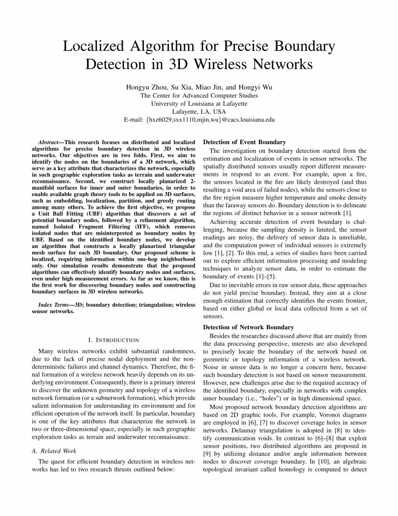
2) Motivations and Theoretic Insights: The proposed UBFalgorithm is motivated by the fact that a hole can alwayscontain an empty unit ball. For example, the smallest holeis defined as a void space that can be filled by adding a nodeto connect with nearby nodes. Therefore, we can search forempty unit balls in order to identify holes and boundary nodes.More specifically, a node can test if it is on a boundary byconstructing a unit ball with itself on the ball’s surface. If atleast one such ball can be found that no nodes are locatedinside, a hole is identified and the node is a boundary node(see Node A in Fig. 2(a) for example).

The above process is called unit ball fitting. It can beapplied to identify both inner and outer boundaries. However,it is obviously infeasible for a node to perform a completetest of unit ball fitting via brute-force search, because thereare infinite possible orientations to place the unit ball. Next,we will show that a localized algorithm with a polynomial

A

r

(a) An empty unit ball touching Node A.

AB

C

(b) Ball rotation.

Fig. 2. Principles for Unit Ball Fitting (UBF).

computing complexity can be employed to test if such anempty unit ball exists.

Lemma 1: Node A can construct an empty unit ball thattouches itself if and only if there exists an empty unit balltouching Node A and two neighbors of Node A (within 2r).

Proof: We first show the sufficient condition, which isstraightforward. If a unit ball touched by Node A and twoneighbors of Node A is empty, i.e., there is an empty unitball with Node A and two neighbors of Node A on its surface,Node A has constructed such an empty unit ball touching itself.Consequently, a hole is identified and Node A is a boundarynode.

Now, we prove the necessary condition. If there exists anempty unit ball with Node A on its surface, we can alwaysfix Node A and rotate the ball until it touches another nodewithin 2r, denoted by Node B (see Fig. 2(b)). Note thatif Node B does not exist, Node A must be isolated, whichconflicts with our assumption of well connected networks (seeDefinition 3). Then we can further rotate the ball with LineAB as an axis, until it touches another node, denoted by NodeC. Similarly, Node C must exist, because otherwise Line AB isdegenerated and thus against Definition 3. Therefore, if NodeA can construct an empty unit ball that touches itself, we canalways find an empty unit ball with Node A and two neighborsof Node A on its surface.

Based on the sufficient condition and the necessary condi-tion discussed above, the lemma is thus proven.

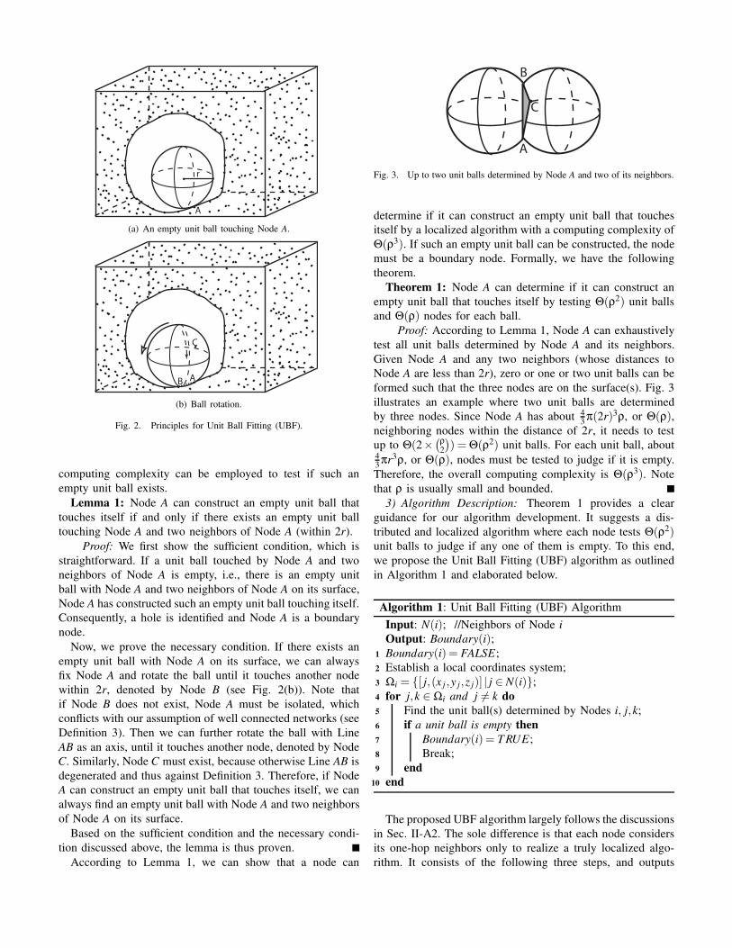
According to Lemma 1, we can show that a node can

A

B

C

Fig. 3. Up to two unit balls determined by Node A and two of its neighbors.

determine if it can construct an empty unit ball that touchesitself by a localized algorithm with a computing complexity of#(!3). If such an empty unit ball can be constructed, the nodemust be a boundary node. Formally, we have the followingtheorem.

Theorem 1: Node A can determine if it can construct anempty unit ball that touches itself by testing #(!2) unit ballsand #(!) nodes for each ball.

Proof: According to Lemma 1, Node A can exhaustivelytest all unit balls determined by Node A and its neighbors.Given Node A and any two neighbors (whose distances toNode A are less than 2r), zero or one or two unit balls can beformed such that the three nodes are on the surface(s). Fig. 3illustrates an example where two unit balls are determinedby three nodes. Since Node A has about 4

3 $(2r)3!, or #(!),neighboring nodes within the distance of 2r, it needs to testup to #(2!

!!2

"

) = #(!2) unit balls. For each unit ball, about43 $r3!, or #(!), nodes must be tested to judge if it is empty.

Therefore, the overall computing complexity is #(!3). Notethat ! is usually small and bounded.

3) Algorithm Description: Theorem 1 provides a clearguidance for our algorithm development. It suggests a dis-tributed and localized algorithm where each node tests #(!2)unit balls to judge if any one of them is empty. To this end,we propose the Unit Ball Fitting (UBF) algorithm as outlinedin Algorithm 1 and elaborated below.

Algorithm 1: Unit Ball Fitting (UBF) Algorithm

Input: N(i); //Neighbors of Node iOutput: Boundary(i);Boundary(i) = FALSE;1

Establish a local coordinates system;2

%i = {[ j,(x j,y j,z j)] | j " N(i)};3

for j,k " %i and j #= k do4

Find the unit ball(s) determined by Nodes i, j,k;5

if a unit ball is empty then6

Boundary(i) = T RUE;7

Break;8

end9

end10

The proposed UBF algorithm largely follows the discussionsin Sec. II-A2. The sole difference is that each node considersits one-hop neighbors only to realize a truly localized algo-rithm. It consists of the following three steps, and outputs

a boolean value Boundary(i) indicating if Node i is on aboundary or not.

(I) Local coordinates establishment (Lines 2-3): If all nodeshave known their coordinates, this step can be skipped.Otherwise each node employs a 3D embedding algorithmto establish a local coordinates system. More specifically,Node i collects the distances between all pairs of nodeswithin one hop. The distance between two nodes can beestimated by such ranging techniques as received signalstrength indicator (RSSI) or time difference of arrival(TDOA) [26]. The measured distances are inaccurate ingeneral and the errors will be discussed in Sec. IV. Basedon the pair-wise distances, multiple schemes [27]–[31]are available to create a local coordinates system forNode i and its neighbors. Among them, [31] is adoptedin our implementation. Once the coordinates system isestablished, Node i keeps a set of neighboring nodesand their coordinates, i.e., %i = {[ j,(x j,y j,z j)] | j "N(i)},where N(i) denotes the set of nodes that include Node iitself and its one-hop neighbors.

(II) Unit ball identification (Lines 4-5): For every two dis-tinct nodes, e.g., j and k " %i, calculate the center(s) ofthe unit ball(s) determined by Nodes i, j and k. This isdone by solving a set of standard equations as follows,where (x,y,z) are the coordinates of the center.

#

$

%

(x$ xi)2 +(y$ yi)2 +(z$ zi)2 = r2,

(x$ x j)2 +(y$ y j)2 +(z$ z j)2 = r2,

(x$ xk)2 +(y$ yk)2 +(z$ zk)2 = r2.

(1)

Depending on the coordinates of Nodes i, j and k, Eq. (1)may yield no solution, or one solution, or two solutionsfor (x,y,z).

(III) Empty unit ball check (Lines 6-9): For each center point(x,y,z) identified above, check if any node in %i islocated inside the corresponding unit ball, i.e., if it isan empty unit ball. If an empty unit ball is found, Nodei declares that it is on a boundary.

Steps (II) and (III) check all unit balls determined by Node i

and its neighbors. If no empty unit ball is found, Node i reportsthat it is not a boundary node. As revealed by Theorem 1, only#(!2) unit balls need to be examined by each node. Moreover,it requires local information only, i.e., merely the coordinatesof the neighboring nodes are needed, and a local coordinatessystem (without global alignment) is sufficient.

In addition, the size of holes to be detected is adjustable byvarying r (or "). By default, one can set r close to 1, in orderto identify the holes of any size. However, if one is interestedin the boundary nodes of large holes only, a larger r can bechosen. As a result, a node on the boundary of a small holecannot find an empty unit ball that can fit in according toAlgorithm 1 and thus deems itself a non-boundary node.

B. Phase 2: Isolated Fragment Filtering (IFF)

A small number of interior nodes may be interpreted byUBF as boundary nodes due to inaccurate nodal coordinates

or unexpected low nodal density areas randomly distributedin the network, resulting in some isolated fragments thatshould be filtered out. Generally, the nodes on a boundaryform a well connected closed surface. Therefore, we can seta threshold &. Any fragment that consists of less than & nodesis not considered as a boundary. To this end, each boundarynode simply initiates a local flooding packet with a TTL ofT , which will be forwarded by other boundary nodes butnot non-boundary nodes. By counting the number of suchflooding packets received, a boundary node learns the sizeof its fragment. If less than & flooding packets are received,the node deems itself a non-boundary node. Appropriate & andT are chosen according to the minimum size of the holes tobe detected. For example, given the default value of r (i.e.,r = 1+" for an arbitrary small "), a minimum hole will haveat least 20 nodes on its surface, forming an icosahedron, wherethe maximum hop distance between two boundary nodes is 3.Thus we set & = 20 and T = 3. Since IFF is based on a simplelocal flooding, it has a complexity of O(1).

In addition, the boundary nodes can be easily grouped,when there are multiple boundaries. Note that, the nodeson a boundary are connected via boundary nodes. In otherwords, there must exist a path between two nodes on thesame boundary, which involves boundary nodes only. For twonodes on different boundaries, such path does not exist, andtheir connection must go through at least one non-boundarynode. Therefore a straightforward scheme (similar to the localflooding approach discussed above) can be employed to groupthe boundary nodes.

C. Summary of Boundary Node Identification

By following the two phases elaborated above, a nodedetermines whether it is on the boundary based on localinformation only. Its performance depends on the accuracyin distance measurement, which is used to establish localcoordinates. As to be discussed in Sec. IV, our simulationsdemonstrate that the proposed algorithms are effective, able toidentify almost all boundary nodes with low miss and mistakenrate, when the distance measurement errors are moderate (asshown Fig. 1(g)). Under high distance measurement errors,the mistaken and missing rates naturally increase. But themistakenly identified boundary nodes are all close to the trueboundary, mostly within one or two hops (see Fig. 1(h)). At thesame time, the missed boundary nodes are uniformly scattered.

A

C

B

!1

(a) Non-boundary node.

A

C

B

>1

(b) Missed boundary node.

Fig. 4. Illustration of a missed boundary node. (a) Node A is not a boundarynode. (b) Node A is a boundary node but cannot be identified by UBF.

Over 95% of such missed boundary nodes can always find atleast one correctly identified boundary node within its onehop neighborhood (as illustrated in Fig. 1(i)). Therefore, theidentified boundary nodes can well represent the networkboundaries. More discussion will be presented in Sec. IV.

III. TRIANGULAR BOUNDARY SURFACE CONSTRUCTION

The boundary nodes identified so far are discrete. Theylargely depict the network boundaries. However, many applica-tions require not only discrete boundary nodes, but also closedboundary surfaces. Moreover, it is highly desirable that suchsurfaces are locally planarized 2-manifold in order to applyavailable 2D graphic tools on 3D surfaces.

In this research we implement an algorithm that constructslocally planarized triangular meshes on the identified 3Dboundaries. We adopt the method proposed in [25] that canproduce a planar subgraph in a 2D network, and extendit to 3D surfaces to achieve complete triangulation withoutdegenerated edges. The algorithm is localized and based onconnectivity only. It consists the following five steps.

(I) Landmark Selection: The boundary nodes employ adistributed algorithm (e.g., [32]) to elect a subset ofnodes as “landmarks”. Any two landmarks must be k-hops apart. k determines the fineness of the mesh. It isusually set between 3 to 5 in our implementation. A non-landmark boundary node is associated with the closestlandmark. If it has the same distance (in hop counts) tomultiple landmarks, it chooses the one with the smallestID as a tiebreaker. This step creates a set of approximateVoronoi cells on each boundary (as shown in Fig. 1(c)).

(II) Construction of Combinatorial Delaunay Graph (CDG):

Each non-landmark boundary node checks if it has aneighboring boundary node that is associated with adifferent landmark. If it has, a message is sent to bothlandmarks to indicate that they are neighboring land-marks. If we simply connect all neighboring landmarks,we arrive at a Combinatorial Delaunay Graph (CDG)as illustrated in Fig 1(d), which is the respective dualof the Voronoi cells on a boundary found in Step I.However, such a CDG is not planar (see the crossingedges highlighted in Fig 1(d)).

(III) Construction of Combinatorial Delaunay Map (CDM):

Each landmark node decides whether it connects to aneighboring landmark as follows. It sends a packet to aneighboring landmark through the shortest path (basedon the identified boundary nodes only). The packetrecords the nodes along the path. The two landmarksare said to be connected if and only if the followingtwo conditions are satisfied. First, all of nodes visitedby the packet are associated to these two landmarksonly. Second, assume the packet is sent from Landmarki to Landmark j. Then the packet must visit the nodesassociated with Landmark i first, and then followed bythe nodes associated with Landmark j, without interleav-ing. If the above two conditions are satisfied, Landmark

A

B

C E

D

(a) Before edge flip.

A

B

C E

D

(b) After edge flip.

Fig. 5. Illustration of edge flip. Edge AB has three faces before edge flip. Itis removed and replaced by Edges CD and DE .

j sends an ACK to Landmark i and a virtual edge isadded between them. The boundary nodes that receivesuch ACK records that they are on the shortest pathbetween two connected landmarks. This step yields aCombinatorial Delaunay Map (CDM). It is proven thatCDM is a planar graph [25].

(IV) Construction of Triangular Mesh: The CDM obtained sofar is planar, but not always a triangular mesh. Polygonswith more than three edges may exist (see the polygonhighlighted in Fig 1(e)). To achieve complete triangula-tion, appropriate edges should be added between someneighboring landmarks. If a landmark, e.g., Landmark i,has a non-connected neighboring landmark (e.g., Land-mark j), it sends a connection packet to the latter (viathe shortest path based on the identified boundary nodes).The packet will be dropped if it reaches an intermediatenode that is already on the shortest path between twoconnected landmarks, in order to avoid crossing edges.If the connection packet arrives at Landmark j, a virtualedge can be safely added and an ACK is sent back toLandmark i. Similarly, the boundary nodes that receivethe ACK records that they are on the shortest pathbetween two connected landmarks. This step adds allpossible virtual edges to divide polygons into triangles.

(V) Edge Flip: To ensure the mesh to be a 2-manifold, eachvirtual edge must be associated with two triangles. Afterthe above step, there still possibly exist edges (like EdgeAB in Fig. 5(a)) with three triangular faces, formed withthree corresponding nodes (i.e., C, D, and E). Such edgescan be detected by trivial local signaling. For each suchedge, a transformation is done as follows. First, EdgeAB is removed. Second, two shortest edges are addedbetween the corresponding nodes, i.e., Nodes C, D, andE . For example, assume CE is longer than CD and DE .Then two virtual edges CD and DE are added, resultingin Fig. 5(b), where no edge has more than two faces.Note that the polygon ACBE is not a face on the surface.Till now, we arrive at a planar triangular mesh for each3D boundary surface, as illustrated in Fig. 1(f).

The above algorithm is able to form a closed triangular meshsurface for each boundary. The established triangular mesh is alocally planarized 2-manifold, although the whole 3D surface

is not planar. A virtual edge on a mesh surface has exactly twotriangular faces. Such salient properties enable application ofmany useful graph theory tools on 3D boundary surfaces, in-cluding embedding, localization, partition, and greedy routingamong many others.

Note that since the triangular mesh is established basedon landmarks only, a small number of nodes (that are onor close to the boundaries) may be located outside the meshsurfaces. The number of such nodes is determined by k andthe curvature of the boundary. The larger the k, the coarserthe mesh surfaces, resulting in more nodes left outside. Anappropriate k can be chosen according to the needs of specificapplications. For example, Fig. 1(f) shows the results withk = 3.

In addition, we observed that the triangular mesh is notseriously deformed under distance measurement errors. Asdiscussed in the previous subsection, the mistakenly identifiedboundary nodes are close to the true boundary and the miss-ing boundary nodes are uniformly distributed. Therefore, theidentified boundary nodes can still well represent the networkboundaries, even under distance measurement errors. This isverified by our simulations. For example, Figs. 1(j)-1(l) showresults under 20%, 30% and 40% distance measurement errors,respectively. They exhibit similar triangular meshs as Fig. 1(j),which is free of distance measurement errors.

IV. SIMULATIONS

To evaluate the effectiveness of our proposed boundary de-tection algorithms, we have carried out extensive simulationsunder various 3D wireless networks and studied the impact ofa wide range of distance measurement errors. In this section,we will first introduce our simulation setup. Then we presentthe simulation results and discuss our observations.

A. Simulation Setup

The 3D networks used in our simulations are constructedby using a set of 3D graphic tools (including TetGen [33]).First, a 3D model is developed to represent a given networkscenario (e.g., an underwater network, a 3D network in space,and general 3D networks with arbitrary shapes of our interest).A set of nodes are randomly uniformly distributed on thesurface of the 3D model. They are marked as boundarynodes, serving as ground truth to evaluate our algorithm.A cloud of nodes are then deployed inside the 3D model.Again the nodes are randomly uniformly distributed. Oncethe nodes are determined, an appropriate radio transmissionrange is chosen according to nodal density, such that thenetwork is connected. Each node connects to its neighborswithin its radio transmission range. In our simulated networks,nodal degree ranges from 5 to 45, with an average of 18.5.A node also estimates its distance to each neighbor. Whileour simulations do not involve physical layer modeling, weintroduce a wide range of random errors, from 0 to 100% ofthe radio transmission radius, in the distance measurement.

Till now, we have the input for our algorithm. For eachsimulated network, the input includes a set of the nodes (both

interior and boundary nodes), the local 1-hop connectivity ofeach node, and the distance measurement (with various errors)within 1-hop neighborhood.

B. Simulation Results

We run our proposed distributed and localized algorithmsfor boundary node detection and surface construction. First,each node establishes a local coordinates system by using dis-tributed multi-dimensional scaling [31] based on local distancemeasurement. Then boundary node identification is performed,followed by the triangular mesh algorithm.

Several examples of our simulated networks are given inFigs. 6-10. Fig. 6 illustrates an underwater network, wherenodes are distributed from the surface to the bottom of theocean. As shown in Figs. 6(b) and 6(c), our algorithmseffectively identify the boundaries of both smooth watersurface and the bumpy bottom. Figs. 7 and 8 depicts a 3Dnetwork deployed in the space (e.g., for chemical dispersionsampling in 3D space). They have one and two internal holes,respectively, due to uncontrolled drift of sensor nodes. Theseexamples demonstrate that our algorithm works for not onlyouter boundary but also the boundaries of interior holes.Figs. 9 and 10 show 3D networks deployed in a bended pipeand a sphere, respectively. As can be seen, boundary nodesare accurately identified and the triangular mesh surfaces arewell constructed in the both networks.

Fig. 11 illustrates the performance statistics obtained fromour simulations. The results are based on over 10,000 sampleboundary nodes. As can be seen in Fig. 11(a), our algorithmperforms almost perfectly to identify boundary nodes whenthe distance measurement error is less than 30%. With moreerrors introduced in distance measurement, noticeable errorsare yielded in local coordinates establishment, which naturallylead to missing and mistaken boundary nodes. More specif-ically, when the coordinates errors exceed certain level, anoriginal boundary node may become an interior node inside thenetwork under the established coordinates and thus is missedby our boundary detection algorithm. At the same time, anoriginal interior node may appear on the boundary due tothe deformation of the coordinates of the node itself and itsneighbors, leading to a mistakenly identified boundary node.However, as we have demonstrated in Fig. 1 and discussedin Sec. II, such missing and mistaken boundary nodes do notseriously affect our boundary identification, because they arewell distributed. For example, Fig. 11(b) illustrates the distri-bution of mistaken boundary nodes. Specifically, we measurethe shortest distance (in hops) from a mistaken boundary nodeto a correctly identified boundary node. As can be seen inFig. 11(b), such distance is always less than 3 hops, witha majority of them in one (over 60%) and two hops (over30%). These results clearly show that the mistakenly identifiednodes are very close to the true boundary. Therefore, thetriangular mesh surface does not deviate significantly from thetrue boundary surface. Similarly, the distribution of missingboundary nodes is given in Fig. 11(c). It is observed that al-most 100% of the missing boundary nodes are within one-hop

(a) Network model. (b) Boundary nodes. (c) Triangular mesh.

Fig. 6. An example of under water network. (In contrast to Figs. 7-10 where the network model, i.e., subfigure (a), shows a set of wireless nodes deployed,the network model in this figure gives the actual 3D model for better visualization.)

(a) Network model. (b) Boundary nodes. (c) Triangular mesh.

Fig. 7. An example of a 3D space network with an internal hole.

(a) Network model. (b) Boundary nodes. (c) Triangular mesh.

Fig. 8. An example of a 3D space network with two internal holes.

(a) Network model. (b) Boundary nodes. (c) Triangular mesh.

Fig. 9. An example of a 3D network in a bended pipe.

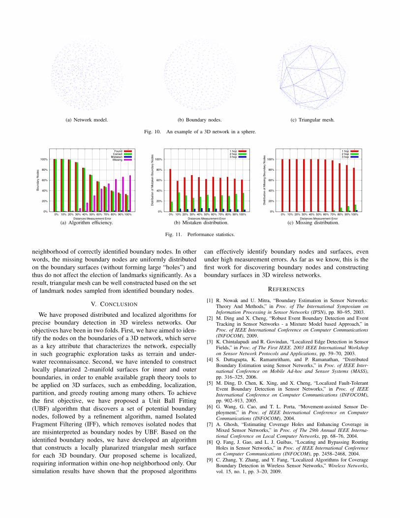
(a) Network model. (b) Boundary nodes. (c) Triangular mesh.

Fig. 10. An example of a 3D network in a sphere.

0%

20%

40%

60%

80%

100%

0% 10% 20% 30% 40% 50% 60% 70% 80% 90% 100%

Boun

dary

Nod

es

Distances Measurement Error

FoundCorrect

MistakenMissing

(a) Algorithm efficiency.

0%

20%

40%

60%

80%

100%

0% 10% 20% 30% 40% 50% 60% 70% 80% 90% 100%

Dis

tribu

tion

of M

ista

ken

Boun

dary

Nod

es

Distances Measurement Error

1 hop2 hop3 hop

(b) Mistaken distribution.

0%

20%

40%

60%

80%

100%

0% 10% 20% 30% 40% 50% 60% 70% 80% 90% 100%

Dis

tribu

tion

of M

issi

ng B

ound

ary

Nod

es

Distances Measurement Error

1 hop2 hop3 hop

(c) Missing distribution.

Fig. 11. Performance statistics.

neighborhood of correctly identified boundary nodes. In otherwords, the missing boundary nodes are uniformly distributedon the boundary surfaces (without forming large “holes”) andthus do not affect the election of landmarks significantly. As aresult, triangular mesh can be well constructed based on the setof landmark nodes sampled from identified boundary nodes.

V. CONCLUSION

We have proposed distributed and localized algorithms forprecise boundary detection in 3D wireless networks. Ourobjectives have been in two folds. First, we have aimed to iden-tify the nodes on the boundaries of a 3D network, which serveas a key attribute that characterizes the network, especiallyin such geographic exploration tasks as terrain and under-water reconnaissance. Second, we have intended to constructlocally planarized 2-manifold surfaces for inner and outerboundaries, in order to enable available graph theory tools tobe applied on 3D surfaces, such as embedding, localization,partition, and greedy routing among many others. To achievethe first objective, we have proposed a Unit Ball Fitting(UBF) algorithm that discovers a set of potential boundarynodes, followed by a refinement algorithm, named IsolatedFragment Filtering (IFF), which removes isolated nodes thatare misinterpreted as boundary nodes by UBF. Based on theidentified boundary nodes, we have developed an algorithmthat constructs a locally planarized triangular mesh surfacefor each 3D boundary. Our proposed scheme is localized,requiring information within one-hop neighborhood only. Oursimulation results have shown that the proposed algorithms

can effectively identify boundary nodes and surfaces, evenunder high measurement errors. As far as we know, this is thefirst work for discovering boundary nodes and constructingboundary surfaces in 3D wireless networks.

REFERENCES

[1] R. Nowak and U. Mitra, “Boundary Estimation in Sensor Networks:Theory And Methods,” in Proc. of The International Symposium onInformation Processing in Sensor Networks (IPSN), pp. 80–95, 2003.

[2] M. Ding and X. Cheng, “Robust Event Boundary Detection and EventTracking in Sensor Networks - a Mixture Model based Approach,” inProc. of IEEE International Conference on Computer Communications(INFOCOM), 2009.

[3] K. Chintalapudi and R. Govindan, “Localized Edge Detection in SensorFields,” in Proc. of The First IEEE. 2003 IEEE International Workshopon Sensor Network Protocols and Applications, pp. 59–70, 2003.

[4] S. Duttagupta, K. Ramamritham, and P. Ramanathan, “DistributedBoundary Estimation using Sensor Networks,” in Proc. of IEEE Inter-national Conference on Mobile Ad-hoc and Sensor Systems (MASS),pp. 316–325, 2006.

[5] M. Ding, D. Chen, K. Xing, and X. Cheng, “Localized Fault-TolerantEvent Boundary Detection in Sensor Networks,” in Proc. of IEEEInternational Conference on Computer Communications (INFOCOM),pp. 902–913, 2005.

[6] G. Wang, G. Cao, and T. L. Porta, “Movement-assisted Sensor De-ployment,” in Proc. of IEEE International Conference on ComputerCommunications (INFOCOM), 2004.

[7] A. Ghosh, “Estimating Coverage Holes and Enhancing Coverage inMixed Sensor Networks,” in Proc. of The 29th Annual IEEE Interna-tional Conference on Local Computer Networks, pp. 68–76, 2004.

[8] Q. Fang, J. Gao, and L. J. Guibas, “Locating and Bypassing RoutingHoles in Sensor Networks,” in Proc. of IEEE International Conferenceon Computer Communications (INFOCOM), pp. 2458–2468, 2004.

[9] C. Zhang, Y. Zhang, and Y. Fang, “Localized Algorithms for CoverageBoundary Detection in Wireless Sensor Networks,” Wireless Networks,vol. 15, no. 1, pp. 3–20, 2009.

[10] R. Ghrist and A. Muhammad, “Coverage and Hole-Detection in SensorNetworks Via Homology,” in Proc. of The International Symposium onInformation Processing in Sensor Networks (IPSN), pp. 254–260, 2005.

[11] S. Funke, “Topological Hole Detection in Wireless Sensor Networks andIts Applications,” in Proc. of Joint Workshop on Foundations of MobileComputing (DIALM-POMC), pp. 44–53, 2005.

[12] A. Kroller, S. P. Fekete, D. Pfisterer, and S. Fischer, “DeterministicBoundary Recognition and Topology Extraction for Large Sensor Net-works,” in Proc. of ACM-SIAM Symposium on Discrete Algorithms(SODA), pp. 1000–1009, 2006.

[13] Y. Wang, J. Gao, and J. S. B. Mitchell, “Boundary Recognition in SensorNetworks by Topological Methods,” in Proc. of The ACM/IEEE Inter-national Conference on Mobile Computing and Networking (MobiCom),pp. 122–133, 2006.

[14] C. Liu and J. Wu, “Efficient Geometric Routing in Three DimensionalAd Hoc Networks,” in Proc. of IEEE International Conference onComputer Communications (INFOCOM), 2009.

[15] T. F. G. Kao and J. Opatmy, “Position-Based Routing on 3D GeometricGraphs in Mobile Ad Hoc Networks,” in Proc. of The 17th CanadianConference on Computational Geometry, pp. 88–91, 2005.

[16] J. Opatrny, A. Abdallah, and T. Fevens, “Randomized 3D Position-basedRouting Algorithms for Ad-hoc Networks,” in Proc. of Third AnnualInternational Conference onMobile and Ubiquitous Systems: Networking& Services, pp. 1–8, 2006.

[17] R. Flury and R. Wattenhofer, “Randomized 3D Geographic Routing,” inProc. of IEEE International Conference on Computer Communications(INFOCOM), pp. 834–842, 2008.

[18] F. Li, S. Chen, Y. Wang, and J. Chen, “Load Balancing Routing inThree Dimensional Wireless Networks,” in Proc. of IEEE InternationalConference on Communications (ICC), pp. 3073–3077, 2008.

[19] D. Pompili, T. Melodia, and I. F. Akyildiz, “Routing Algorithmsfor Delay-insensitive and Delay-sensitive Applications in UnderwaterSensor Networks,” in Proc. of The ACM/IEEE International Conferenceon Mobile Computing and Networking (MobiCom), pp. 298–309, 2006.

[20] W. Cheng, A. Y. Teymorian, L. Ma, X. Cheng, X. Lu, and Z. Lu,“Underwater localization in sparse 3d acoustic sensor networks,” inProc. of IEEE International Conference on Computer Communications(INFOCOM), pp. 798–806, 2008.

[21] X. Bai, C. Zhang, D. Xuan, J. Teng, and W. Jia, “Low-Connectivityand Full-Coverage Three Dimensional Networks,” in Proc. of ACMInternational Symposium on Mobile Ad hoc Networking and Computing(MobiHOC), pp. 145–154, 2009.

[22] X. Bai, C. Zhang, D. Xuan, and W. Jia, “Full-Coverage and K-Connectivity (K=14, 6) Three Dimensional Networks,” in Proc. of IEEEInt’l Conference on Computer Communications (INFOCOM), 2009.

[23] J. Allred, A. B. Hasan, S. Panichsakul, W. Pisano, P. Gray, J. Huang,R. Han, D. Lawrence, and K. Mohseni, “SensorFlock: An AirborneWireless Sensor Network of Micro-Air Vehicles,” in Proc. of The Inter-national Conference on Embedded Networked Sensor Systems (SenSys),pp. 117–129, 2007.

[24] J.-H. Cui, J. Kong, M. Gerla, and S. Zhou, “Challenges: BuildingScalable Mobile Underwater Wireless Sensor Networks for Aquatic Ap-plications,” IEEE Network, Special Issue on Wireless Sensor Networking,vol. 20, no. 3, pp. 12–18, 2006.

[25] S. Funke and N. Milosavljevi, “How Much Geometry Hides in Con-nectivity? - Part II,” in Proc. of ACM-SIAM Symposium on DiscreteAlgorithms (SODA), pp. 958–967, 2007.

[26] Z. Zhong and T. He, “MSP: Multi-Sequence Positioning of WirelessSensor Nodes,” in Proc. of The International Conference on EmbeddedNetworked Sensor Systems (SenSys), pp. 15–28, 2007.

[27] H. Wu, C. Wang, and N.-F. Tzeng, “Novel Self-Configurable PositioningTechnique for Multi-hop Wireless Networks,” IEEE/ACM Transactionson Networking, vol. 13, no. 3, pp. 609–621, 2005.

[28] G. Giorgetti, S. Gupta, and G. Manes, “Wireless Localization UsingSelf-Organizing Maps,” in Proc. of The International Symposium onInformation Processing in Sensor Networks (IPSN), pp. 293 – 302, 2007.

[29] L. Li and T. Kunz, “Localization Applying An Efficient Neural NetworkMapping,” in Proc. of The 1st International Conference on AutonomicComputing and Communication Systems, pp. 1–9, 2007.

[30] Y. Shang, W. Ruml, Y. Zhang, and M. P. J. Fromherz, “Localizationfrom Mere Connectivity,” in Proc. of ACM Int’l Symposium on MobileAd hoc Networking and Computing (MobiHOC), pp. 201–212, 2003.

[31] Y. Shang and W. Ruml, “Improved MDS-based Localization,” in Proc.

of IEEE International Conference on Computer Communications (IN-FOCOM), pp. 2640–2651, 2004.

[32] Q. Fang, J. Gao, L. J. Guibas, V. Silva, and L. Zhang, “GLIDER:Gradient Landmark-based Distributed Routing for Sensor Networks,” inProc. of IEEE International Conference on Computer Communications(INFOCOM), pp. 339–350, 2005.

[33] http://tetgen.berlios.de/.