locally adaptive metrics for clustering high dimensional data

Locally Adaptive Metrics for Clustering High

Dimensional Data

Carlotta DomeniconiGeorge Mason University

Dimitrios GunopulosUC Riverside

Sheng MaIBM T.J. Watson Research Center

Dimitris PapadopoulosUC Riverside

Bojun YanGeorge Mason University

Abstract. Clustering suffers from the curse of dimensionality, and similarity func-tions that use all input features with equal relevance may not be effective. Weintroduce an algorithm that discovers clusters in subspaces spanned by differentcombinations of dimensions via local weightings of features. This approach avoids therisk of loss of information encountered in global dimensionality reduction techniques,and does not assume any data distribution model. Our method associates to eachcluster a weight vector, whose values capture the relevance of features within thecorresponding cluster. We experimentally demonstrate the gain in perfomance ourmethod achieves with respect to competitive methods, using both synthetic and realdatasets. In particular, our results show the feasibility of the proposed technique toperform simultaneous clustering of genes and conditions in gene expression data,and clustering of very high dimensional data such as text data.

Keywords: subspace clustering, dimensionality reduction, local feature relevance,gene expression data, text data.

1. Introduction

The clustering problem concerns the discovery of homogeneous groupsof data according to a certain similarity measure. It has been studiedextensively in statistics (Arabie and Hubert, 1996), machine learning(Cheeseman and Stutz, 1996; Michalski and Stepp, 1996), and databasecommunities (Ng and Han, 1994; Ester et al., 1995; Zhang et al., 1996).

Given a set of multivariate data, (partitional) clustering finds a par-tition of the points into clusters such that the points within a clusterare more similar to each other than to points in different clusters. Thepopular K-means or K-medoids methods compute one representativepoint per cluster, and assign each object to the cluster with the closest

2 Carlotta Domeniconi et al.

representative, so that the sum of the squared differences between theobjects and their representatives is minimized. Finding a set of repre-sentative vectors for clouds of multi-dimensional data is an importantissue in data compression, signal coding, pattern classification, andfunction approximation tasks.

Clustering suffers from the curse of dimensionality problem in highdimensional spaces. In high dimensional spaces, it is highly likely that,for any given pair of points within the same cluster, there exist at leasta few dimensions on which the points are far apart from each other.As a consequence, distance functions that equally use all input featuresmay not be effective.

Furthermore, several clusters may exist in different subspaces,comprised of different combinations of features. In many real worldproblems, in fact, some points are correlated with respect to a givenset of dimensions, and others are correlated with respect to differentdimensions. Each dimension could be relevant to at least one of theclusters.

The problem of high dimensionality could be addressed by requiringthe user to specify a subspace (i.e., subset of dimensions) for clusteranalysis. However, the identification of subspaces by the user is an error-prone process. More importantly, correlations that identify clusters inthe data are likely not to be known by the user. Indeed, we desire suchcorrelations, and induced subspaces, to be part of the findings of theclustering process itself.

An alternative solution to high dimensional settings consists inreducing the dimensionality of the input space. Traditional featureselection algorithms select certain dimensions in advance. Methods suchas Principal Component Analysis (PCA) (or Karhunen-Loeve transfor-mation) (Duda and Hart, 1973; Fukunaga, 1990) transform the originalinput space into a lower dimensional space by constructing dimensionsthat are linear combinations of the given features, and are orderedby nonincreasing variance. While PCA may succeed in reducing thedimensionality, it has major drawbacks. The new dimensions can bedifficult to interpret, making it hard to understand clusters in relationto the original space. Furthermore, all global dimensionality reductiontechniques (like PCA) are not effective in identifying clusters that mayexist in different subspaces. In this situation, in fact, since data acrossclusters manifest different correlations with features, it may not alwaysbe feasible to prune off too many dimensions without incurring a loss ofcrucial information. This is because each dimension could be relevantto at least one of the clusters.

These limitations of global dimensionality reduction techniques sug-gest that, to capture the local correlations of data, a proper feature

Locally Adaptive Metrics for Clustering High Dimensional Data 3

selection procedure should operate locally in input space. Local featureselection allows to embed different distance measures in different re-gions of the input space; such distance metrics reflect local correlationsof data. In this paper we propose a soft feature selection procedurethat assigns (local) weights to features according to the local corre-lations of data along each dimension. Dimensions along which dataare loosely correlated receive a small weight, that has the effect ofelongating distances along that dimension. Features along which dataare strongly correlated receive a large weight, that has the effect ofconstricting distances along that dimension. Figure 1 gives a simpleexample. The left plot depicts two clusters of data elongated alongthe x and y dimensions. The right plot shows the same clusters, wherewithin-cluster distances between points are computed using the respec-tive local weights generated by our algorithm. The weight values reflectlocal correlations of data, and reshape each cluster as a dense sphericalcloud. This directional local reshaping of distances better separatesclusters, and allows for the discovery of different patterns in differentsubspaces of the original input space.

-10-9-8-7-6-5-4-3-2-10123456789

10

-3 -2 -1 0 1 2 3 4 5 6 7 8 9 10 11 12 13 14 15 16 17 18 19 20

y

x

Cluster0 in original input spaceCluster1 in original input space

-10-9-8-7-6-5-4-3-2-10123456789

10

-3 -2 -1 0 1 2 3 4 5 6 7 8 9 10 11 12 13 14 15 16 17 18 19 20

y

x

Cluster0 transformed by local weightsCluster1 transformed by local weights

Figure 1. (Left) Clusters in original input space. (Right) Clusters transformed bylocal weights.

1.1. Our Contribution

An earlier version of this work appeared in (Domeniconi et al., 2004).However, this paper is a substantial extension, which includes (as newmaterial) a new derivation and motivation of the proposed algorithm,a proof of convergence of our approach, a variety of experiments, com-parisons, and analysis using high-dimensional text and gene expressiondata. Specifically, the contributions of this paper are as follows:

1. We formalize the problem of finding different clusters in differentsubspaces. Our algorithm (Locally Adaptive Clustering, or LAC)discovers clusters in subspaces spanned by different combinationsof dimensions via local weightings of features. This approach avoids


the risk of loss of information encountered in global dimensionalityreduction techniques.

2. The output of our algorithm is twofold. It provides a partition ofthe data, so that the points in each set of the partition constitutea cluster. In addition, each set is associated with a weight vector,whose values give information of the degree of relevance of featuresfor each partition.

3. We formally prove that our algorithm converges to a local minimumof the associated error function, and experimentally demonstratethe gain in perfomance we achieve with our method. In particular,our results show the feasibility of the proposed technique to performsimultaneous clustering of genes and conditions in gene expressiondata, and clustering of very high dimensional data such as textdata.

2. Related Work

Local dimensionality reduction approaches for the purpose of efficientlyindexing high dimensional spaces have been recently discussed in thedatabase literature (Keogh et al., 2001; Chakrabarti and Mehrotra,2000; Thomasian et al., 1998). Applying global dimensionality re-duction techniques when data are not globally correlated can causesignificant loss of distance information, resulting in a large numberof false positives and hence a high query cost. The general approachadopted by the authors is to find local correlations in the data, andperform dimensionality reduction on the locally correlated clustersindividually. For example, in (Chakrabarti and Mehrotra, 2000), theauthors first construct spacial clusters in the original input space usinga simple tecnique that resembles K-means. Principal component analy-sis is then performed on each spatial cluster individually to obtain theprincipal components.

In general, the efficacy of these methods depends on how the clus-tering problem is addressed in the first place in the original featurespace. A potential serious problem with such techniques is the lack ofdata to locally perform PCA on each cluster to derive the principalcomponents. Moreover, for clustering purposes, the new dimensionsmay be difficult to interpret, making it hard to understand clusters inrelation to the original space.

The problem of finding different clusters in different subspaces of theoriginal input space has been addressed in (Agrawal et al., 1998). The


authors use a density based approach to identify clusters. The algorithm(CLIQUE) proceeds from lower to higher dimensionality subspaces anddiscovers dense regions in each subspace. To approximate the densityof the points, the input space is partitioned into cells by dividing eachdimension into the same number ξ of equal length intervals. For agiven set of dimensions, the cross product of the corresponding intervals(one for each dimension in the set) is called a unit in the respectivesubspace. A unit is dense if the number of points it contains is abovea given threshold τ . Both ξ and τ are parameters defined by the user.The algorithm finds all dense units in each k-dimensional subspace bybuilding from the dense units of (k−1)-dimensional subspaces, and thenconnects them to describe the clusters as union of maximal rectangles.

While the work in (Agrawal et al., 1998) successfully introduces amethodology for looking at different subspaces for different clusters, itdoes not compute a partitioning of the data into disjoint groups. Thereported dense regions largely overlap, since for a given dense region allits projections on lower dimensionality subspaces are also dense, andthey all get reported. On the other hand, for many applications suchas customer segmentation and trend analysis, a partition of the data isdesirable since it provides a clear interpretability of the results.

Recently (Procopiuc et al., 2002), another density-based projectiveclustering algorithm (DOC/FastDOC) has been proposed. This ap-proach requires the maximum distance between attribute values (i.e.maximum width of the bounding hypercubes) as parameter in input,and pursues an optimality criterion defined in terms of density of eachcluster in its corresponding subspace. A Monte Carlo procedure is thendeveloped to approximate with high probability an optimal projectivecluster. In practice it may be difficult to set the parameters of DOC,as each relevant attribute can have a different local variance.

(Dy and Brodley, 2000) also addresses the problem of feature se-lection to find clusters hidden in high dimensional data. The authorssearch through feature subset spaces, evaluating each subset by firstclustering in the corresponding subspace, and then evaluating the re-sulting clusters and feature subset using the chosen feature selectioncriterion. The two feature selection criteria investigated are the scat-ter separability used in discriminant analysis (Fukunaga, 1990), anda maximum likelihood criterion. A sequential forward greedy strategy(Fukunaga, 1990) is employed to search through possible feature sub-sets. We observe that dimensionality reduction is performed globallyin this case. Therefore, the technique in (Dy and Brodley, 2000) isexpected to be effective when a dataset contains some relevant featuresand some irrelevant (noisy) ones, across all clusters.


The problem of finding different clusters in different subspaces is alsoaddressed in (Aggarwal et al., 1999). The proposed algorithm (PRO-jected CLUStering) seeks subsets of dimensions such that the pointsare closely clustered in the corresponding spanned subspaces. Both thenumber of clusters and the average number of dimensions per clusterare user-defined parameters. PROCLUS starts with choosing a randomset of medoids, and then progressively improves the quality of medoidsby performing an iterative hill climbing procedure that discards the’bad’ medoids from the current set. In order to find the set of dimen-sions that matter the most for each cluster, the algorithm selects thedimensions along which the points have the smallest average distancefrom the current medoid. ORCLUS (Aggarwal and Yu, 2000) modifiesthe PROCLUS algorithm by adding a merging process of clusters, andselecting for each cluster principal components instead of attributes.

In contrast to the PROCLUS algorithm, our method does not re-quire to specify the average number of dimensions to be kept per cluster.For each cluster, in fact, all features are taken into consideration, butproperly weighted. The PROCLUS algorithm is more prone to loss ofinformation if the number of dimensions is not properly chosen. Forexample, if data of two clusters in two dimensions are distributed asin Figure 1 (Left), PROCLUS may find that feature x is the mostimportant for cluster 0, and feature y is the most important for cluster1. But projecting cluster 1 along the y dimension doesn’t allow toproperly separate points of the two clusters. We avoid this problemby keeping both dimensions for both clusters, and properly weightingdistances along each feature within each cluster.

The problem of feature weighting in K-means clustering has beenaddressed in (Modha and Spangler, 2003). Each data point is repre-sented as a collection of vectors, with “homogeneous” features withineach measurement space. The objective is to determine one (global)weight value for each feature space. The optimality criterion pursuedis the minimization of the (Fisher) ratio between the average within-cluster distortion and the average between-cluster distortion. However,the proposed method does not learn optimal weights from the data.Instead, different weight value combinations are ran through a K-means-like algorithm, and the combination that results in the lowestFisher ratio is chosen. We also observe that the weights as defined in(Modha and Spangler, 2003) are global, in constrast to ours which arelocal to each cluster.

Recently (Dhillon et al., 2003), a theoretical formulation of sub-space clustering based on information theory has been introduced. Thedata contingency matrix (e.g., document-word co-occurrence matrix) isseen as an empirical joint probability distribution of two discrete ran-


dom variables. Subspace clustering is then formulated as a constrainedoptimization problem where the objective is to maximize the mutualinformation between the clustered random variables.

Generative approaches have also been developed for local dimen-sionality reduction and clustering. The approach in (Ghahramani andHinton, 1996) makes use of maximum likelihood factor analysis tomodel local correlations between features. The resulting generativemodel obeys the distribution of a mixture of factor analyzers. Anexpectation-maximization algorithm is presented for fitting the param-eters of the mixture of factor analyzers. The choice of the number offactor analyzers, and the number of factors in each analyzer (that drivesthe dimensionality reduction) remain an important open issue for theapproach in (Ghahramani and Hinton, 1996).

(Tipping and Bishop, 1999) extends the single PCA model to amixture of local linear sub-models to capture nonlinear structure inthe data. A mixture of principal component analyzers model is derivedas a solution to a maximum-likelihood problem. An EM algorithm isformulated to estimate the parameters.

While the methods in (Ghahramani and Hinton, 1996; Tipping andBishop, 1999), as well as the standard mixture of Gaussians technique,are generative and parametric, our approach can be seen as an attemptto directly estimate from the data local correlations between features.Furthermore, both mixture models in (Ghahramani and Hinton, 1996;Tipping and Bishop, 1999) inherit the soft clustering component of theEM update equations. On the contrary, LAC computes a partitioningof the data into disjoint groups. As previously mentioned, for manydata mining applications a partition of the data is desirable since itprovides a clear interpretability of the results. We finally observe that,while mixture of Gaussians models, with arbitrary covariance matrices,could in principle capture local correlations along any directions, lackof data to locally estimate full covariance matrices in high dimensionalspaces is a serious problem in practice.

2.1. Biclustering of Gene Expression Data

Microarray technology is one of the latest breakthroughs in experi-mental molecular biology. Gene expression data are generated by DNAchips and other microarray techniques, and they are often presented asmatrices of expression levels of genes under different conditions (e.g.,environment, individuals, tissues). Each row corresponds to a gene, andeach column represents a condition under which the gene is developed.

Biologists are interested in finding set of genes showing strikinglysimilar up-regulation and down-regulation under a set of conditions.


To this extent, recently the concept of bicluster has been introduced(Cheng and Church, 2000). A bicluster is a subset of genes and a sub-set of conditions with a high similarity score. A particular score thatapplies to expression data is the mean squared residue score (Chengand Church, 2000). Let I and J be subsets of genes and experimentsrespectively. The pair (I, J) specifies a submatrix AIJ with a meansquared residue score defined as follows:

H(I, J) =1

|I||J |∑

i∈I,j∈J

(aij − aiJ − aIj + aIJ)2, (1)

where aiJ = 1|J |

∑j∈J aij , aIj = 1

|I|∑

i∈I aij, and aIJ =1

|I||J |∑

i∈I,j∈J aij . They represent the row and column means, and themean of the submatrix, respectively. The lowest score H(I, J) = 0indicates that the gene expression levels fluctuate in unison. The aimis then to find biclusters with low mean squared residue score (below acertain threshold).

We observe that the mean squared residue score is minimized whensubsets of genes and experiments (or dimensions) are chosen so that thegene vectors (i.e., rows of the resulting bicluster) are close to each otherwith respect to the Euclidean distance. As a result, the LAC algorithm,and other subspace clustering algorithms, are well suited to performsimultaneous clustering of both genes and conditions in a microarraydata matrix. (Wang et al., 2002) introduces an algorithm (pCluster) forclustering similar patterns, that has been applied to DNA microarraydata of a type of yeast. The pCluster model optimizes a criterion that isdifferent from the mean squared residue score, as it looks for coherentpatterns on a subset of dimensions (e.g., in an identified subspace,objects reveal larger values for the second dimension than for the first).

3. Locally Adaptive Metrics for Clustering

We define what we call weighted cluster. Consider a set of points insome space of dimensionality N . A weighted cluster C is a subset ofdata points, together with a vector of weights w = (w1, . . . , wN ), suchthat the points in C are closely clustered according to the L2 normdistance weighted using w. The component wj measures the degree ofcorrelation of points in C along feature j. The problem becomes nowhow to estimate the weight vector w for each cluster in the dataset.

In this setting, the concept of cluster is not based only on points, butalso involves a weighted distance metric, i.e., clusters are discovered inspaces transformed by w. Each cluster is associated with its own w,


that reflects the correlation of points in the cluster itself. The effect ofw is to transform distances so that the associated cluster is reshapedinto a dense hypersphere of points separated from other data.

In traditional clustering, the partition of a set of points is inducedby a set of representative vectors, also called centroids or centers. Thepartition induced by discovering weighted clusters is formally definedas follows.Definition: Given a set S of D points x in the N -dimensional Eu-clidean space, a set of k centers {c1, . . . , ck}, cj ∈ �N , j = 1, . . . , k,coupled with a set of corresponding weight vectors {w1, . . . ,wk},wj ∈ �N , j = 1, . . . , k, partition S into k sets {S1, . . . , Sk}:

Sj = {x|(N∑

i=1

wji(xi − cji)2)1/2 < (N∑

i=1

wli(xi − cli)2)1/2,∀l �= j}, (2)

where wji and cji represent the ith components of vectors wj and cj

respectively (ties are broken randomly).The set of centers and weights is optimal with respect to the

Euclidean norm, if they minimize the error measure:

E1(C,W ) =k∑

j=1

N∑

i=1

(wji1

|Sj|∑

x∈Sj

(cji − xi)2) (3)

subject to the constraints∑

i wji = 1 ∀j. C and W are (N×k) matriceswhose column vectors are cj and wj respectively, i.e. C = [c1 . . . ck] andW = [w1 . . .wk]. For shortness of notation, we set

Xji =1

|Sj|∑

x∈Sj

(cji − xi)2,

where |Sj| is the cardinality of set Sj . Xji represents the average dis-tance from the centroid cj of points in cluster j along dimension i. Thesolution

(C∗,W ∗) = argmin(C,W )E1(C,W )

will discover one dimensional clusters: it will put maximal (i.e., unit)weight on the feature with smallest dispersion Xji within each clusterj, and zero weight on all other features. Our objective, instead, is tofind weighted multidimensional clusters, where the unit weight getsdistributed among all features according to the respective dispersionof data within each cluster. One way to achieve this goal is to addthe regularization term

∑Ni=1 wjilogwji

1, which represents the nega-tive entropy of the weight distribution for each cluster (Friedman and

1 Different regularization terms lead to different weighting schemes.


Meulman, 2002). It penalizes solutions with maximal (unit) weight onthe single feature with smallest dispersion within each cluster. Theresulting error function is

E2(C,W ) =k∑

j=1

N∑

i=1

(wjiXji + hwjilogwji) (4)

subject to the same constraints∑

i wji = 1 ∀j. The coefficient h ≥ 0 is aparameter of the procedure; it controls the relative differences betweenfeature weights. In other words, h controls how much the distribution ofweight values will deviate from the uniform distribution. We can solvethis constrained optimization problem by introducing the Lagrangemultipliers λj (one for each constraint), and minimizing the resulting(unconstrained now) error function

E(C,W ) =k∑

j=1

N∑

i=1

(wjiXji + hwjilogwji) +k∑

j=1

λj(1 −N∑

i=1

wji) (5)

For a fixed partition P and fixed cji, we compute the optimal w∗ji by

setting ∂E∂wji

= 0 and ∂E∂λj

= 0. We obtain:

∂E

∂wji= Xji + hlogwji + h − λj = 0 (6)

∂E

∂λj= 1 −

N∑

i=1

wji = 0 (7)

Solving equation (6) with respect to wji we obtain hlogwji = −Xji +λj − h. Thus:

wji = exp(−Xji/h + (λj/h) − 1) = exp(−Xji/h)exp((λj/h) − 1)

=exp(−Xji/h)exp(1 − λj/h)

.

Substituting this expression in equation (7):

∂E

∂λj= 1−

N∑

i=1

exp(−Xji/h)exp(1 − λj/h)

= 1− 1exp(−λj/h)

N∑

i=1

exp((−Xji/h) − 1) = 0.

Solving with respect to λj we obtain

λj = −hlogN∑

i=1

exp((−Xji/h) − 1).


Thus, the optimal w∗ji is

w∗ji =

exp(−Xji/h)exp(1 + log(

∑Ni=1 exp((−Xji/h) − 1)))

=exp(−Xji/h)

∑Ni=1 exp(−Xji/h)

(8)

For a fixed partition P and fixed wji, we compute the optimal c∗ji bysetting ∂E

∂cji= 0. We obtain:

∂E

∂cji= wji

1|Sj |2

∑

x∈Sj

(cji − xi) =2wji

|Sj | (|Sj |cji −∑

x∈Sj

xi) = 0.

Solving with respect to cji gives

c∗ji =1

|Sj |∑

x∈Sj

xi. (9)

Solution (8) puts increased weight on features along which the disper-sion Xji is smaller, within each cluster. The degree of this increaseis controlled by the value h. Setting h = 0, places all weight on thefeature i with smallest Xji, whereas setting h = ∞ forces all fea-tures to be given equal weight for each cluster j. By setting E0(C) =1N

∑kj=1

∑Ni=1 Xji, we can formulate this result as follows.

Proposition: When h = 0, the error function E2 (4) reduces to E1

(3); when h = ∞, the error function E2 reduces to E0.

4. Locally Adaptive Clustering Algorithm

We need to provide a search strategy to find a partition P that identifiesthe solution clusters. Our approach progressively improves the qualityof initial centroids and weights, by investigating the space near thecenters to estimate the dimensions that matter the most. Specifically,we proceed as follows.

We start with well-scattered points in S as the k centroids: wechoose the first centroid at random, and select the others so that theyare far from one another, and from the first chosen center. We initiallyset all weights to 1/N . Given the initial centroids cj , for j = 1, . . . , k,we compute the corresponding sets Sj as given in the definition above.We then compute the average distance Xji along each dimension fromthe points in Sj to cj . The smaller Xji is, the larger is the correlationof points along dimension i. We use the value Xji in an exponential


weighting scheme to credit weights to features (and to clusters), asgiven in equation (8). The exponential weighting is more sensitiveto changes in local feature relevance (Bottou and Vapnik, 1992) andgives rise to better performance improvement. Note that the techniqueis centroid-based because weightings depend on the centroid. Thecomputed weights are used to update the sets Sj, and therefore thecentroids’ coordinates as given in equation (9). The procedure isiterated until convergence is reached. The resulting algorithm, that wecall LAC (Locally Adaptive Clustering), is summarized in the following.

Input: D points x ∈ RN , k, and h.

1. Start with k initial centroids c1, c2, . . . , ck;

2. Set wji = 1/N , for each centroid cj , j = 1, . . . , k and each featurei = 1, . . . , N ;

3. For each centroid cj , and for each point x:

− Set Sj = {x|j = arg minl Lw(cl,x)},where Lw(cl,x) = (

∑Ni=1 wli(cli − xi)2)1/2;

4. Compute new weights.For each centroid cj , and for each feature i:

− Set Xji =∑

x∈Sj(cji − xi)2/|Sj |;

Set wji = exp(−Xji/h)∑N

l=1exp(−Xjl/h)

;

5. For each centroid cj , and for each point x:

− Recompute Sj = {x|j = arg minl Lw(cl,x)};6. Compute new centroids.

Set cj =∑

xx1Sj

(x)∑x

1Sj(x)

, for each j = 1, . . . , k, where 1S(.) is the

indicator function of set S;

7. Iterate 3,4,5,6 until convergence.

The sequential structure of the LAC algorithm is analogous to themathematics of the EM algorithm (Dempster et al., 1977; Wu, 1983).The hidden variables are the assignments of the points to the centroids.Step 3 constitutes the E step: it finds the values of the hidden variablesSj given the previous values of the parameters wji and cji. The followingstep (M step) consists in finding new matrices of weights and centroidsthat minimize the error function with respect to the current estimation


of hidden variables. It can be shown that the LAC algorithm convergesto a local minimum of the error function (5). The running time of oneiteration is O(kDN).

We point out that the LAC algorithm can identify a degeneratesolution, i.e. a partition with empty clusters, during any iteration. Al-though we didn’t encounter this problem in our experiments, strategiesdeveloped in the literature, such as the insertion strategy (Mladenovicand Brimberg, 1996), can be easily incorporated in our algorithm. Inparticular, we can proceed as follows: if the number of non-empty clus-ters in the current iteration of LAC is l < k, we can identify the l pointswith the leargest (weighted) distance to their cluster’s centroid, andform l new clusters with a single point in each of them. The resultingnon-degenerate solution is clearly better than the degenerate one sincethe selected l points give the largest contributions to the cost function,but it could possibly be improved. Therefore, the LAC iterations cancontinue until convergence to a non-degenerate solution.

5. Convergence of the LAC Algorithm

In light of the remark made above on the analogy of LAC with EM(Wu, 1983), here we prove that our algorithm converges to a solutionthat is a local minimum of the error function (5). To obtain this resultwe need to show that the error function decreases at each iteration ofthe algorithm. By derivation of equations (8) and (9), Step 4 and Step6 of the LAC algorithm perform a gradient descent over the surface ofthe error function (5). We make use of this observation to show thateach iteration of the algorithm decreases the error function. We provethe following theorem.Theorem. The LAC algorithm converges to a local minimum of theerror function (5).Proof. For a fixed partition P and fixed cji, the optimal w′

ji obtainedby setting ∂E

∂wji= 0 and ∂E

∂λj= 0 is:

w′ji =

exp(−Xji/h)∑N

l=1 exp(−Xjl/h)(10)

as in Step 4 of the LAC algorithm.For a fixed partition P and fixed wji, the optimal c′ji obtained by

setting ∂E∂cji

= 0 is:

c′ji =1

|Sj |∑

x∈Sj

xi (11)


as in Step 6 of the LAC algorithm.The algorithm consists in repeatedly replacing wji and cji with w′

jiand c′ji using equations (10) and (11), respectively. The value of theerror function E at completion of each iteration is EP1(C

′,W ′), wherewe explicit the dependence of E on the partition of points P1 computedin Step 5 of the algorithm. C ′ and W ′ are the matrices of the newlycomputed centroids and weights. Since the new partition P ′ computedin Step 3 of the successive iteration is by definition the best assignmentof points x to the centroids c′ji according to the weighted Euclideandistance with weights w′

ji, we have the following inequality:

EP ′(C ′,W ′) − EP1(C′,W ′) ≤ 0 (12)

Using this result, and the identities E(C ′,W ′) = EP ′(C ′,W ′) andE(C,W ) = EP (C,W ), we can derive the following inequality:

E(C ′,W ′) − E(C,W ) = EP ′(C ′,W ′) − EP1(C′,W ′)

+ EP1(C′,W ′) − EP (C,W )

≤ EP1(C′,W ′) − EP (C,W ) ≤ 0

where the last inequality is derived by using the definitions of w′ji and

c′ji.Thus, each iteration of the algorithm decreases the lower bounded

error function E (5) until the error reaches a fixed point where condi-tions w∗′

j = w∗j , c∗′j = c∗j ∀j are verified. The fixed points w∗

j and c∗jgive a local minimum of the error function E.

6. Experimental Evaluation

In our experiments we have designed five different simulated datasets tocompare the competitive algorithms under different conditions. Clus-ters are distributed according to multivariate gaussians with differentmean and standard deviation vectors. We have tested problems withtwo and three clusters up to 50 dimensions. For each problem, wehave generated five or ten training datasets, and for each of them anindependent test set. In the following we report accuracy and perfor-mance results obtained via 5(10)-fold cross-validation comparing LAC,PROCLUS, DOC, K-means, and EM (Dempster et al., 1977) (mixtureof Gaussians with diagonal - EM(d) - and full - EM(f) - covariancematrices). Among the subspace clustering techniques available in theliterature, we chose PROCLUS (Aggarwal et al., 1999) and DOC (Pro-copiuc et al., 2002) since, as the LAC algorithm, they also compute apartition of the data. On the contrary, the CLIQUE technique (Agrawal


et al., 1998) allows overlapping between clusters, and thus its resultsare not directly comparable with ours.

Error rates are computed according to the confusion matrices thatare also reported. For LAC we tested the integer values from 1 to 11for the parameter 1/h, and report the best error rates achieved. Thek centroids are initialized by choosing well-scattered points among thegiven data. The mean vectors and covariance matrices provided byK-means are used to initialize the parameters of EM.

6.1. Simulated Data

1. Example1. The dataset consists of N = 2 input features and k = 3clusters. All three clusters are distributed according to multivariategaussians. Mean vector and standard deviations for one cluster are(2, 0) and (4, 1) respectively. For the second cluster the vectors are(10, 0) and (1, 4), and for the third are (18, 0) and (4, 1). Table I showsthe results for this problem. We generated 60000 data points, andperformed 10-fold cross-validation with 30000 training data and 30000testing data.2. Example2. This dataset consists of N = 30 input features andk = 2 clusters. Both clusters are distributed according to multivariategaussians. Mean vector and standard deviations for one cluster are(1, . . . , 1) and (10, 5, 10, 5, . . . , 10, 5), respectively. For the other clusterthe vectors are (2, 1, . . . , 1) and (5, 10, 5, 10, . . . , 5, 10). Table I showsthe results for this problem. We generated 10000 data points, andperformed 10-fold cross-validation with 5000 training and 5000 testingdata.3. Example3. This dataset consists of N = 50 input features andk = 2 clusters. Both clusters are distributed according to multivari-ate gaussians. Mean vector and standard deviations for one clusterare (1, . . . , 1) and (20, 10, 20, 10, . . . , 20, 10), respectively. For the othercluster the vectors are (2, 1, . . . , 1) and (10, 20, 10, 20, . . . , 10, 20). TableI shows the results for this problem. We generated 10000 data points,and performed 10-fold cross-validation with 5000 training data and5000 testing data.4. Example4. This dataset consists of off-axis oriented clusters, withN = 2 and k = 2. Figure 3 shows the distribution of the points for thisdataset. We generated 20000 data points, and performed 5-fold-cross-validation with 10000 training data and 10000 testing data. Table Ishows the results.5. Example5. This dataset consists again of off-axis oriented two di-mensional clusters. This dataset contains three clusters, as Figure 4


depicts. We generated 30000 data points, and performed 5-fold-cross-validation with 15000 training data and 15000 testing data. Table Ishows the results.

6.2. Real Data

We used ten real datasets. The OQ-letter, Wisconsin breast cancer,Pima Indians Diabete, and Sonar data are taken from the UCI Ma-chine Learning Repository. The Image data set is obtained from theMIT Media Lab. We used three high dimensional text datasets: Clas-sic3, Spam2000, and Spam5996. The documents in each dataset werepreprocessed by eliminating stop words (based on a stop words list),and stemming words to their root source. We use as feature valuesfor the vector space model the frequency of the terms in the corre-sponding document. The Classic3 dataset is a collection of abstractsfrom three categories: MEDLINE (abstracts from medical journals),CISI (abstracts from IR papers), CRANFIELD (abstracts from aero-dynamics papers). The Spam data belong to the Email-1431 dataset.This dataset consists of emails falling into three categories: conference(370), jobs (272), and spam (786). We run two different experimentswith this dataset. In one case we reduce the dimensionality to 2000terms (Spam2000), in the second case to 5996 (Spam5996). In bothcases we consider two clusters by merging the conference and jobs mailsinto one group (non-spam). The characteristics of these eight datasetsare as follows. OQ: D = 1536, N = 16, k = 2; Breast: D = 683,N = 9, k = 2; Pima: D = 768, N = 8, k = 2; Image: D = 640, N = 16,k = 15; Sonar: D = 208, N = 60, k = 2; Classic3: D = 3893, N = 3302,k = 3; Spam2000: D = 1428, N = 2000, k = 2; Spam5996: D = 1428,N = 5996, k = 2. To study whether our projected clustering algorithmis applicable to gene expression profiles, we used two datasets: the B-cell lymphoma (Alizadeh et al., 2000) and the DNA microarray of geneexpression profiles in hereditary breast cancer (Hedenfalk et al., 2001).The lymphoma dataset contains 96 samples, each with 4026 expressionvalues. We clustered the samples with the expression values of thegenes as attributes (4026 dimensions). The samples are categorizedinto 9 classes according to the category of mRNA sample studied. Weused the class labels to compute error rates, according to the confusionmatrices. We also experiment our algorithm with a DNA microarraydataset (Hedenfalk et al., 2001). The microarray contains expressionlevels of 3226 genes under 22 conditions. We clustered the genes withthe expression values of the samples as attributes (22 dimensions). Thedataset is presented as a matrix: each row corresponds to a gene, andeach column represents a condition under which the gene is developed.


Table I. Average error rates for simulated data.

LAC PROCLUS K-means DOC EM (d) EM (f)

Ex1 11.4±0.3 13.8±0.7 24.2±0.5 35.2± 2.2 5.1 ± 0.4 5.1 ± 0.4

Ex2 0.5±0.4 27.9±9.8 48.4±1.1 no clusters 0.6 ±0.3 0.8 ±0.3

Ex3 0.08±0.1 21.6±5.3 48.1±1.1 no clusters 0.0 ±0.1 25.5 ±0.2

Ex4 4.8±0.4 7.1±0.7 7.7±0.7 22.7± 5.9 4.8 ± 0.2 2.3 ± 0.2

Ex5 7.7±0.3 7.0±2.0 18.7±2.7 16.5± 3.9 6.0 ± 0.2 2.3 ± 0.2

Average 4.9 15.5 29.4 24.8 3.3 7.2

Biologists are interested in finding set of genes showing strikinglysimilar up-regulation and down-regulation under a set of conditions.Since class labels are not available for this dataset, we utilize the meansquared residue score as defined in (1) to assess the quality of theclusters detected by LAC and PROCLUS algorithms. The lowest scorevalue 0 indicates that the gene expression levels fluctuate in unison.The aim is to find biclusters with low mean squared residue score (ingeneral, below a certain threshold).

Table II. Average number of iterations.

LAC PROCLUS K-means EM(d)

Ex1 7.2 6.7 16.8 22.4

Ex2 3.2 2.0 16.1 6.3

Ex3 3.0 4.4 19.4 6.0

Ex4 7.0 6.4 8.0 5.6

Ex5 7.8 9.8 15.2 27.6

Average 5.6 5.9 15.1 13.6

6.3. Results on Simulated Data

The performance results reported in Table I clearly demonstrate thelarge gain in performance obtained by the LAC algorithm with respectto PROCLUS and K-means with high dimensional data. The goodperformance of LAC on Examples 4 and 5 shows that our algorithm isable to detect clusters folded in subspaces not necessarily aligned withthe input axes. Figures 5 and 6 illustrate the results obtained with


Table III. Dimensions selected by PROCLUS.

C0 C1 C2

Ex1 2,1 2,1 2,1

Ex2 8,30 19,15,21,1,27,23 -

Ex3 50,16 50,16,17,18,21,22,23,19,11,3 -

Ex4 1,2 2,1 -

Ex5 1,2 2,1 1,2

2526272829303132333435363738394041424344454647484950

1 2 3 4 5 6 7 8 9 10 11 12 13 14 15 16

Err

or R

ate

Average Number of Dimensions

Figure 2. Example2: Error rate of PROCLUS versus Average number of dimensions.

Table IV. Confusion matrices for Example1.

LAC C0 (input) C1 (input) C2 (input)

C0 (output) 8315 0 15

C1 (output) 1676 10000 1712

C2 (output) 9 0 8273

PROCLUS C0 (input) C1 (input) C2 (input)

C0 (output) 7938 0 7

C1 (output) 2057 10000 2066

C2 (output) 5 0 7927

K-means C0 (input) C1 (input) C2 (input)

C0 (output) 9440 4686 400

C1 (output) 411 3953 266

C2 (output) 149 1361 9334


Table V. LAC: Weight values for Ex-ample1.

Cluster Std1 Std2 w1 w2

C0 4 1 0.46 0.54

C1 1 4 0.99 0.01

C2 4 1 0.45 0.55

LAC and K-means, respectively, on Example 5. The large error ratesof K-means for the 30 and 50 dimensional datasets (Examples 2 and3) show how ineffective a distance function that equally use all inputfeatures can be in high dimensional spaces. Example 1, 2, and 3 offeroptimal conditions for EM(d); Example 4 and 5 are optimal for EM(f).As a consequence, EM(d) and EM(f) provide best error rates in suchrespective cases. Nevertheless, LAC gives error rates similar to EM(d)under conditions which are optimal for the latter, especially in higherdimensions. The large error rate of EM(f) for Example 3 shows thedifficulty of estimating full covariance matrices in higher dimensions.

PROCLUS requires the average number of dimensions per clusteras parameter in input; its value has to be at least two. We have cross-validated this parameter and report the best error rates obtained inTable I. PROCLUS is able to select highly relevant features for datasetsin low dimensions, but fails to do so in higher dimensions, as the largeerror rates for Examples 2 and 3 show. Table III shows the dimensionsselected by PROCLUS for each dataset and each cluster. Figure 2 plotsthe error rate as a function of the average number of dimensions percluster, obtained by running PROCLUS on Example 2. The best errorrate (27.9%) is achieved in correspondence of the value four. The errorrate worsens for larger values of the average number of dimensions.Figure 2 shows that the performance of PROCLUS is highly sensi-tive to the value of its input parameter. If the average number ofdimensions is erroneously estimated, the performance of PROCLUSsignificantly worsens. This can be a serious problem with real data,when the required parameter value is most likely unknown.

We set the parameters of DOC as suggested in (Procopiuc et al.,2002). DOC failed to find any clusters in the high dimensional examples.It is particularly hard to set the input parameters of DOC, as localvariances of features are unknown in practice.

Table II shows the average number of iterations performed by LAC,K-means, and EM(d) to achieve convergence, and by PROCLUS toachieve the termination criterion. For each problem, the rate of con-


vergence of LAC is superior to the rate of K-means: on Examples 1through 5 the speed-ups are 2.3, 5.0, 6.5, 1.1, and 1.9 respectively. Thenumber of iterations performed by LAC and PROCLUS is close foreach problem, and the running time of an iteration of both algorithmsis O(kDN) (where k is the number of clusters, D is the number of datapoints, and N the number of dimensions). The faster rate of conver-gence achieved by the LAC algorithm with respect to K-means (andEM(d)) is motivated by the exponential weighting scheme provided byequation (8), which gives the optimal weight values w∗

ji. Variations ofthe within-cluster dispersions Xji (along each dimension i) are expo-nentially reflected into the corresponding weight values wji. Thus the(exponential) weights are more sensitive (than quadratic or linear ones,for example) to changes in local feature relevance. As a consequence, aminimum value of the error function (5) can be reached in less iterationsthan the corresponding unweighted cost function minimized by theK-means algorithm.

To further test the accuracy of the algorithms, for each problemwe have computed the confusion matrices. The entry (i, j) in eachconfusion matrix is equal to the number of points assigned to outputcluster i, that were generated as part of input cluster j. We also reportthe average weight values per cluster obtained over the runs conductedin our experiments. Results are reported in Tables IV-XI.

Tables V, IX, and XI show that there is a perfect correspondencebetween the weight values of each cluster and the correlation patternsof data within the same cluster. This is of great importance for ap-plications that require not only a good partitioning of data, but alsoinformation to what features are relevant for each partition.

As expected, the resulting weight values for one cluster depends onthe configurations of other clusters as well. If clusters have the samestandard deviation along one dimension i, they receive almost identicalweights for measuring distances along that feature. This is informativeof the fact that feature i is equally relevant for both partitions. On theother hand, weight values are largely differentiated when two clustershave different standard deviation values along the same dimension i,implying different degree of relevance of feature i for the two partitions(see for example Table V).

6.4. Results on Real Data

Table XII reports the error rates obtained on the nine real datasetswith class labels. For LAC we fixed the value of the parameter 1/hto 9 (this value gave in general good results with the simulated data).We ran PROCLUS with input parameter values from 2 to N for each


dataset, and report the best error rate obtained in each case. For theLymphoma (4026 dimensions), Classic3 (3302 dimensions), Spam2000(2000 dimensions), and Spam5996 (5996 dimensions) we tested severalinput parameter values of PROCLUS, and found the best result at3500, 350, 170, and 300 respectively. LAC gives the best error ratein seven out of the nine datasets. LAC outperforms PROCLUS andEM(d) in each dataset. EM does not perform well in general, andparticularly in higher dimensions. This is likely due to the non-Gaussiandistributions of real data. EM(f) (Netlab library for Matlab) failed torun to completion on the very high dimensional data due to memoryproblems. In three cases (Breast, Pima, Image), LAC and K-meanshave very similar error rates. For these sets, LAC did not find localstructures in the data, and credited approximately equal weights tofeatures. K-means performs poorly on the OQ and Sonar data. Theenhanced performance given by the subspace clustering techniques inthese two cases suggest that data are likely to be locally correlated.This seems to be true also for the Lymphoma data. The LAC algorithmdid extremely well on the three high dimensional text data (Classic3,Spam2000, and Spam5996), which demostrate the capability of LACin finding meaningful local structure in high dimensional spaces. Thisresult suggests that an analysis of the weights credited to terms canguide the automatic identification of class-specific keywords, and thusthe process of label assignment to clusters.

The DOC algorithm performed poorly, and failed to find any clusterson the very high dimensional data (Lymphoma, Classic3, Spam2000,and Spam5996). We did extensive testing for different parameter values,and report the best error rates in Table XII. For the OQ data, we testedwidth values from 0.1 to 3.4 (at steps of 0.1). (The two actual clustersin this dataset have standard deviation values along input features inthe ranges (0.7, 3.2) and (0.95, 3.2).) The best result obtained reportedone cluster only, and 63.0% error rate. We also tried a larger widthvalue (6), and obtained one cluster again, and error rate 54.0%. Forthe Sonar data we obtained the best result reporting two clusters fora width value of 0.5. Though, the error rate is still very high (65%).We tested several other values (larger and smaller), but they all failedto finding any cluster in the data. (The two actual clusters in thisdataset have standard deviation values along input features in theranges (0.005, 0.266) and (0.0036, 0.28).) These results clearly show thedifficulty of using the DOC algorithm in practice.

We capture robustness of a technique by computing the ratio bm

of its error rate em and the smallest error rate over all methods beingcompared in a particular example: bm = em/min1≤k≤4 ek. Thus, thebest method m∗ for an example has bm∗ = 1, and all other methods


have larger values bm ≥ 1, for m �= m∗. The larger the value of bm, theworse the performance of method m is in relation to the best one forthat example, among the methods being compared. The distributionof the bm values for each method m over all the examples, therefore,seems to be a good indicator concerning its robustness. For example, if aparticular method has an error rate close to the best in every problem,its bm values should be densely distributed around the value 1. Anymethod whose b value distribution deviates from this ideal distributionreflect its lack of robustness. Figure 10 plots the distribution of bm

for each method over the six real datasets OQ, Breast, Pima, Image,Sonar and Lymphoma. For scaling issues, we plot the distribution ofbm for each method over the three text data separately in Figure 11.For each method (LAC, PROCLUS, K-means, EM(d)) we stack the sixbm values. (We did not consider DOC since it failed to find reasonablepatterns in most cases.) LAC is the most robust technique among themethods compared. In particular, Figure 11 graphically depicts thestrikingly superior performance of LAC over the text data with respectto the competitive techniques.

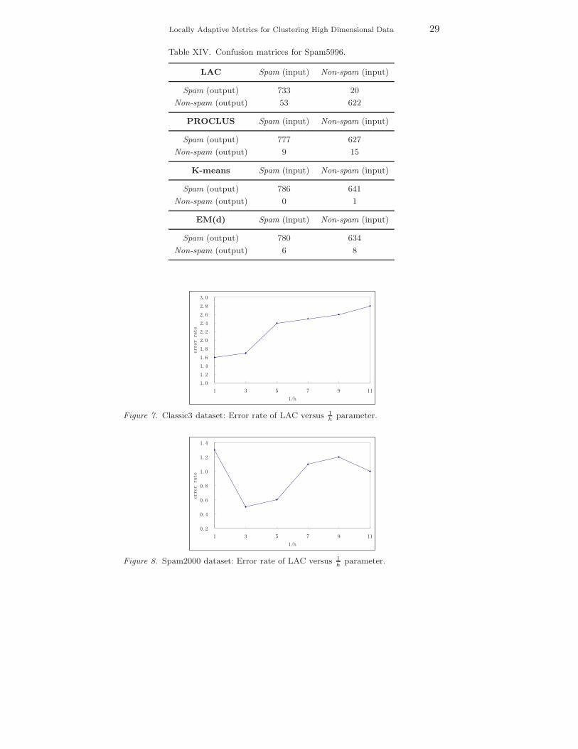
To investigate the false positive and false negative rates on the spamdata we show the corresponding confusion matrices in Tables XIII andXIV. In both cases, LAC has low false positive (FP ) and low falsenegative (FN) rates. On Spam2000: FP = 0.26%, FN = 2.3% OnSpam5996: FP = 2.66%, FN = 7.85%. PROCLUS discovers, to someextent, the structure of the two groups for Spam2000 (FP = 18.8%,FN = 35.1%), but fails completely for Spam5996. This result confirmsour findings with the simulated data, i.e., PROCLUS fails to selectrelevant features in high dimensions. In both cases, K-means and EM(d)are unable to discover the two groups in the data: almost all emails areclustered in a single group. In Figures 7-9 we plot the error rate of LACas a function of the input parameter h for the three text datasets usedin our experiments. As expected, the accuracy of the LAC algorithmis sensitive to the value of h; nevertheless, a good performance wasachieved across the range of values tested ( 1

h = 1, 3, 5, 7, 9, 11).We run the LAC and PROCLUS algorithms using the microarray

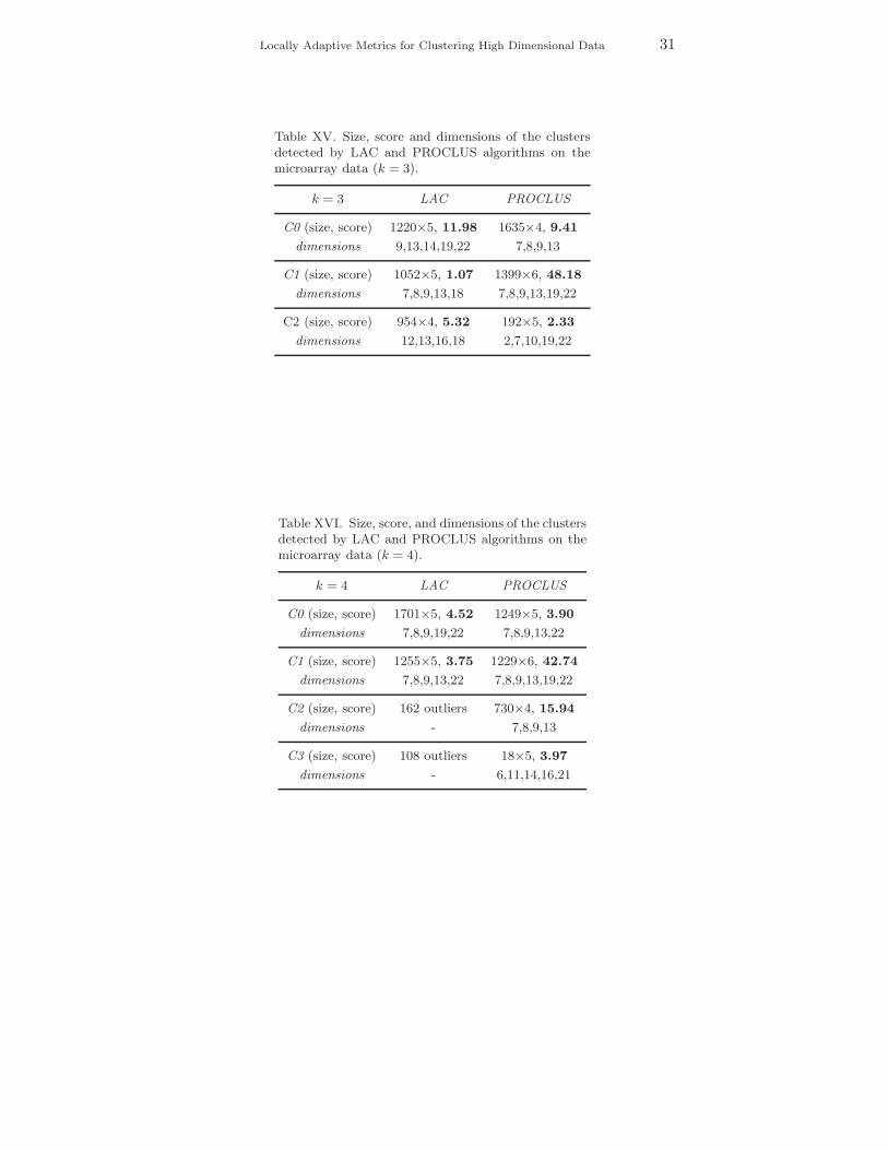
data and small values of k (k = 3 and k = 4). Tables XV and XVI showsizes, scores, and dimensions of the biclusters detected by LAC andPROCLUS. For this dataset, DOC was not able to find any clusters. ForLAC we have selected the dimensions with the largest weights (1/h isfixed to 9). For k = 3, within each cluster four or five conditions receivedsignificant larger weight than the remaining ones. Hence, we selectedthose dimensions. By taking into consideration this result, we run PRO-CLUS with five as value of its input parameter. For k = 4, within twoclusters five conditions receive again considerably larger weight than


the others. The remaining two clusters contain fewer genes, and allconditions receive equal weights. Since no correlation was found amongthe conditions in these two cases, we have “labeled” the correspondingtuples as outliers.

Different combinations of conditions are selected for different biclus-ters, as also expected from a biological perspective. Some conditions areoften selected, by both LAC and PROCLUS (e.g., conditions 7,8, and9). The mean squared residue scores of the biclusters produced by LACare consistently low, as desired. On the contrary, PROCLUS providessome clusters with higher scores (C1 in both Tables XV and XVI).

In general, the weighting of dimensions provides a convenient schemeto properly tune the results. That is: by ranking the dimensions accord-ing to their weight, we can keep adding to a cluster the dimension thatminimizes the increase in score. Thus, given an upper bound on thescore, we can obtain the largest set of dimensions that satisfies thegiven bound.

To assess the biological significance of generated clusters we used abiological data mart (developed by our collaborator biologists), thatemploys an agent framework to maintain knowledge from externaldatabases. Significant themes were observed in some of these groups.For example, one cluster (shown in Table XVII) contains a number ofcell cycle genes. The terms for cell cycle regulation all score high. Aswith all cancers, BRCA1- and BRCA2-related tumors involve the lossof control over cell growth and proliferation, thus the presence of strongcell-cycle components in the clustering is expected.

7. Conclusions and Future Work

We have formalized the problem of finding different clusters in differentsubspaces. Our algorithm discovers clusters in subspaces spanned bydifferent combinations of dimensions via local weightings of features.This approach avoids the risk of loss of information encountered inglobal dimensionality reduction techniques.

The output of our algorithm is twofold. It provides a partition ofthe data, so that the points in each set of the partition constitute acluster. In addition, each set is associated with a weight vector, whosevalues give information of the degree of relevance of features for eachpartition. Our experiments show that there is a perfect correspondencebetween the weight values of each cluster and local correlations of data.

We have formally proved that our algorithm converges to a localminimum of the associated error function, and experimentally demon-strated the gain in perfomance we achieve with our method in high


dimensional spaces with clusters folded in subspaces spanned by differ-ent combinations of features. In addition, we have shown the feasibilityof our technique to discover “good” biclusters in microarray geneexpression data.

The LAC algorithm performed extremely well on the three highdimensional text data (Classic3, Spam2000, and Spam5996). In ourfuture work we will further investigate the use of LAC for keywordidentification of unlabeled documents. An analysis of the weights cred-ited to terms can guide the automatic identification of class-specifickeywords, and thus the process of label assignment to clusters. Thesefindings can have a relevant impact for the retrieval of information incontent-based indexed documents.

The LAC algorithm requires as input parameter the value of h,which controls the strength of the incentive for clustering on more fea-tures. To generate robust and stable solutions, new consensus subspaceclustering methods are under investigation by the authors. The majordifficulty is to find a consensus partition from the output partitions ofthe contributing clusterings, so that an “improved” overall clustering ofthe data is achieved. Since we are dealing with weighted clusters, properconsensus functions that make use of the weight vectors associated withthe clusters will be investigated.

Table VI. Confusion matrices for Exam-ple2.

LAC C0 (input) C1 (input)

C0 (output) 2486 13

C1 (output) 14 2487

PROCLUS C0 (input) C1 (input)

C0 (output) 1755 648

C1 (output) 745 1852

K-means C0 (input) C1 (input)

C0 (output) 1355 1273

C1 (output) 1145 1227


Table VII. Confusion matrices for Exam-ple3.


C0 (output) 2497 1

C1 (output) 3 2499


C0 (output) 2098 676

C1 (output) 402 1824


C0 (output) 1267 1171

C1 (output) 1233 1329

1

2

3

4

5

6

7

8

1 2 3 4 5 6 7 8

y

x

Cluster0Cluster1

Figure 3. Example4: Two Gaussian clusters non-axis oriented in two dimensions.

1

2

3

4

5

6

7

8

1 2 3 4 5 6 7 8

y

x

Cluster0Cluster2Cluster1

Figure 4. Example5: Three Gaussian clusters non-axis oriented in two dimensions.


1

2

3

4

5

6

7

8

1 2 3 4 5 6 7 8y

x


Figure 5. Example5: Clustering results of the LAC algorithm.

1

2

3

4

5

6

7

8

1 2 3 4 5 6 7 8

y

x


Figure 6. Example5: Clustering results of K-means.

Table VIII. Confusion matrices for Exam-ple4.


C0 (output) 4998 473

C1 (output) 2 4527


C0 (output) 5000 714

C1 (output) 0 4286


C0 (output) 4956 724

C1 (output) 44 4276


Table IX. LAC: Weightvalues for Example4.

Cluster w1 w2

C0 0.99 0.01

C1 0.09 0.91

Table X. Confusion matrices for Example5.

LAC C0 (input) C1 (input) C2 (input)

C0 (output) 5000 622 0

C1 (output) 0 3844 0

C2 (output) 0 534 5000

PROCLUS C0 (input) C1 (input) C2 (input)

C0 (output) 5000 712 0

C1 (output) 0 4072 117

C2 (output) 0 216 4883

K-means C0 (input) C1 (input) C2 (input)

C0 (output) 4816 1018 0

C1 (output) 140 3982 1607

C2 (output) 44 0 3393

Table XI. LAC: Weightvalues for Example5.

Cluster w1 w2

C0 0.92 0.08

C1 0.44 0.56

C2 0.94 0.06


Table XII. Average error rates for real data.

LAC PROCLUS K-means DOC EM (d) EM (f)

OQ 30.9 31.6 47.1 54.0 40.0 43.8Breast 4.5 5.7 4.5 32.9 5.3 5.4Pima 29.6 33.1 28.9 42.7 33.7 34.9Image 39.1 42.5 38.3 45.8 39.8 34.6Sonar 38.5 39.9 46.6 65.0 44.5 44.3

Lymphoma 32.3 33.3 39.6 – 47.4 –Classic3 2.6 48.2 62.4 – 59.2 –

Spam2000 1.2 28.0 44.7 – 36.6 –Spam5996 5.1 44.5 44.9 – 44.8 –

Average 20.4 34.1 39.7 48.1 39.0 32.6

Table XIII. Confusion matrices for Spam2000.

LAC Spam (input) Non-spam (input)

Spam (output) 771 2

Non-spam (output) 15 640

PROCLUS Spam (input) Non-spam (input)

Spam (output) 502 116


K-means Spam (input) Non-spam (input)



EM(d) Spam (input) Non-spam (input)




Table XIV. Confusion matrices for Spam5996.

LAC Spam (input) Non-spam (input)



PROCLUS Spam (input) Non-spam (input)



K-means Spam (input) Non-spam (input)



EM(d) Spam (input) Non-spam (input)



Figure 7. Classic3 dataset: Error rate of LAC versus 1h

parameter.

Figure 8. Spam2000 dataset: Error rate of LAC versus 1h

parameter.


Figure 9. Spam5996 dataset: Error rate of LAC versus 1h

parameter.

Figure 10. Performance distributions over real datasets.

Figure 11. Performance distributions over text data.


Table XV. Size, score and dimensions of the clustersdetected by LAC and PROCLUS algorithms on themicroarray data (k = 3).

k = 3 LAC PROCLUS

C0 (size, score) 1220×5, 11.98 1635×4, 9.41

dimensions 9,13,14,19,22 7,8,9,13

C1 (size, score) 1052×5, 1.07 1399×6, 48.18

dimensions 7,8,9,13,18 7,8,9,13,19,22

C2 (size, score) 954×4, 5.32 192×5, 2.33

dimensions 12,13,16,18 2,7,10,19,22

Table XVI. Size, score, and dimensions of the clustersdetected by LAC and PROCLUS algorithms on themicroarray data (k = 4).

k = 4 LAC PROCLUS

C0 (size, score) 1701×5, 4.52 1249×5, 3.90

dimensions 7,8,9,19,22 7,8,9,13,22

C1 (size, score) 1255×5, 3.75 1229×6, 42.74

dimensions 7,8,9,13,22 7,8,9,13,19,22

C2 (size, score) 162 outliers 730×4, 15.94

dimensions - 7,8,9,13

C3 (size, score) 108 outliers 18×5, 3.97

dimensions - 6,11,14,16,21


Table XVII. Biological processes annotated in one cluster generated by the LAC algorithm.

Biological process z-score Biological process z-score

DNA damage checkpoint 7.4 purine nucleotide biosynthesis 4.1

nucleocytoplasmic transport 7.4 mRNA splicing 4.1

meiotic recombination 7.4 cell cycle 3.5

asymmetric cytokinesis 7.4 negative regulation of cell proliferation 3.4

purine base biosynthesis 7.4 induction of apoptosis by intracellular signals 2.8

GMP biosynthesis 5.1 oncogenesis 2.6

rRNA processing 5.1 G1/S transition of mitotic cell cycle 2.5

glutamine metabolism 5.1 protein kinase cascade 2.5

establishment and/or 5.1 central nervous system 4.4maintenance of cell polarity development

gametogenesis 5.1 regulation of cell cycle 2.1

DNA replication 4.6 cell cycle arrest 4.4

glycogen metabolism 2.3


References

Aggarwal, C., Procopiuc, C., Wolf, J. L., Yu, P. S., and Park, J. S. Fast Algo-rithms for Projected Clustering. Proceedings of the ACM SIGMOD InternationalConference on Management of Data, 1999.

Aggarwal, and Yu, P. S. Finding generalized projected clusters in high dimen-sional spaces. Proceedings of the ACM SIGMOD International Conference onManagement of Data, 2000.

Agrawal, R., Gehrke, J., Gunopulos, D., and Raghavan, P. Automatic SubspaceClustering of High Dimensional Data for Data Mining Applications. Proceedingsof the ACM SIGMOD International Conference on Management of Data, 1998.

Alizadeh, A., et al. Distinct types of diffuse large b-cell lymphoma identified by geneexpression profiling. Nature, 403(6769):503–511, 2000.

Arabie, P., and Hubert, L. J. An overview of combinatorial data analysis. Clusteringand Classification. World Scientific Pub., pages 5–63, 1996.

Bottou, L., and Vapnik, V. Local learning algorithms. Neural computation, 4(6):888–900, 1992.

Chakrabarti, K., and Mehrotra, S. Local dimensionality reduction: a new approachto indexing high dimensional spaces. Proceedings of VLDB, 2000.

Cheng, Y., and Church, G. M. Biclustering of expression data. Proceedings of theeighth international conference on intelligent systems for molecular biology, 2000.

Cheeseman, P., and Stutz, J. Bayesian classification (autoclass): theory and results.Advances in Knowledge Discovery and Data Mining, Chapter 6, pages 153–180,AAAI/MIT Press, 1996.

Dempster, A. P., Laird, N. M., and Rubin, D. B. Maximum Likelihood from In-complete Data via the EM Algorithm. Journal of the Royal Statistical Society,39(1):1–38, 1977.

Dhillon, I. S., Mallela, S., and Modha, D. S. Information-theoretic co-clustering.Proceedings of the ACM SIGMOD International Conference on Management ofData, 2003.

Domeniconi, C., Papadopoulos, D., Gunopulos, D., and Ma, S. Subspace Clusteringof High Dimensional Data. Proceedings of the SIAM International Conferenceon Data Mining, 2004.

Duda, R. O., and Hart, P. E. Pattern Classification and Scene Analysis. John Wileyand Sons, 1973.

Dy, J. G., and Brodley, C. E. Feature Subset Selection and Order Identification forUnsupervised Learning. Proceedings of the International Conference on MachineLearning, 2000.

Ester, M., Kriegel, H. P., and Xu, X. A database interface for clustering in large spa-tial databases. Proceedings of the 1st Int’l Conference on Knowledge Discoveryin Databases and Data Mining, 1995.

Friedman, J., and Meulman, J. Clustering Objects on Subsets of Attributes.Technical Report, Stanford University, September 2002.

Fukunaga, K. Introduction to Statistical Pattern Recognition. Academic Press,1990.

Ghahramani, Z., and Hinton, G. E. The EM Algorithm for Mixtures of FactorAnalyzers. Technical Report CRG-TR-96-1, Department of Computer Science,University of Toronto, 1996.

Hedenfalk, I., Duggan, D., Chen, Y., Radmacher, M., Bittner, M., Simon, R.,Meltzer, P., Gusterson, B., Esteller, M., Kallioniemi, O. P., Wilfond, B., Borg,


A., and Trent, J. Gene expression profiles in hereditary breast cancer. N Engl JMed, 344:539–548, 2001.

Keogh, E., Chakrabarti, K., Mehrotra, S., and Pazzani, M. Locally adaptive dimen-sionality reduction for indexing large time series databases. Proceedings of theACM SIGMOD Conference on Management of Data, 2001.

Michalski, R. S., and Stepp, R. E. Learning from observation: Conceptual clustering.Machine Learning: An Artificial Intelligence Approach, in R. S. Michalski, J. G.Carbonell, and T. M. Mitchell editors, 1996.

Mladenovic, N., and Brimberg, J. A degeneracy property in continuous location-allocation problems. Les Cahiers du GERAD, G-96-37, Montreal, Canada, 1996.

Modha, D., and Spangler, S. Feature Weighting in K-Means Clustering. MachineLearning, 52(3):217–237, 2003.

Ng, R. T., and Han, J. Efficient and effective clustering methods for spatial datamining. Proceedings of the VLDB conference, 1994.

Procopiuc, C. M., Jones, M., Agarwal, P. K., and Murali, T. M. A Monte Carloalgorithm for fast projective clustering. Proceedings of the ACM SIGMODConference on Management of Data, 2002.

Tipping, M. E., and Bishop, C. M. Mixtures of Principal Component Analyzers.Neural Computation, 1(2):443–482, 1999.

Thomasian, A., Castelli, V., and Li, C. S. Clustering and singular value decomposi-tion for approximate indexing in high dimensional spaces. Proceedings of CIKM,1998.

Wang, H., Wang, W., Yang, J., and Yu, P. S. Clustering by pattern similarity inlarge data sets. Proceedings of the ACM SIGMOD Conference on Managementof Data, 2002.

Wu, C. F. J. On the convergence properties of the EM algorithm. Annals ofStatistics, 11(1):95–103, 1983.

Zhang, T., Ramakrishnan, R., and Livny, M. BIRCH: An efficient data clusteringmethod for very large databases. Proceedings of the ACM SIGMOD Conferenceon Management of Data, 1996.

locally adaptive metrics for clustering high dimensional data

Documents