location in ad hoc networks

Location in Ad Hoc Networks 619

Location in Ad Hoc Networks

Israel Martin-Escalona, Marc Ciurana and Francisco Barcelo-Arroyo

X

Location in Ad Hoc Networks

Israel Martin-Escalona, Marc Ciurana and Francisco Barcelo-Arroyo Universitat Politecnica de Catalunya (UPC)

Spain

1. Introduction

An ad hoc1 network is defined as a decentralised wireless network that is set up on-the-fly for a specific purpose. These networks were proposed years ago for military use, with the purpose of communicating devices in a highly constrained scenario. Under such a network, devices join and leave the network dynamically; thus, it cannot be expected to have any kind of network infrastructure. This wish for decentralised on-the-fly networks has subsequently expanded to cover several fields besides the military. Today, there are several mobile services requiring the self-organising capabilities that ad hoc networks offer. Examples include packet tracking, online-gaming, and measuring systems, among others. Ad hoc networks have obvious benefits for mobile services, but they also introduce new issues that regular network protocols cannot cope with, including optimum routing, network fragmentation, reduced calculation power, energy-constrained terminals, etc. In ad hoc networks, positioning takes a significant role, mainly due to the on-the-fly condition. In fact, several services require nodes to know the position of the customers in order to perform their duty properly. Wireless sensor networks concentrate most of the services that need positioning to perform their duty. Such networks constitute a subset of ad hoc networks involving dense topologies operating in an ad hoc fashion, and they are composed of small, energy and computation constrained terminals. In ad hoc networks, and especially in wireless sensor networks, nodes are spread over a certain area without a precise knowledge about the topology. In fact, this topology is variable. Accordingly, there are several unknowns (e.g., node density and coverage, network’s energy map, the presence of shadowed zones, nodes’ placement in the network coverage area) that are likely to constrain the performance of ad hoc services. Knowledge of the terminals’ locations can substantially improve the service performance. Positioning is not only important for the service provisioning; it is also crucial in the ad hoc protocol stack development. Due to the changes in the topology and the lack of communication infrastructure, ad hoc protocols have to address several issues not present in regular cellular networks. Routing is one of the best examples of the dependence of ad hoc networks on positioning. Studies such as (Stojmenovic, 2002) demonstrate that only position-based routing protocols are scalable, i.e., able to cope with a higher density of

1 "Ad hoc" is actually a Latin phrase that means "to this (thing, purpose, end, etc.)"

31

www.intechopen.com

Radio Communications620

nodes in the network. The same seems to apply to other management and operation tasks in ad hoc networks.

1.1 The Location problem in ad hoc networks Nodes in an ad hoc network can be grouped into three categories according to the positioning capabilities: beacon nodes, settled nodes, and unknown nodes. Beacon nodes, also known as anchors or landmarks, are those able to compute their position on their own, i.e., without using an ad hoc location algorithm. Accordingly, they implement at least one location technique (e.g., GPS, map matching), which can be used as standalone. Beacon nodes usually constitute the reference frame necessary to set up a location algorithm. Unknown nodes are those nodes that do not know their position yet. When an ad hoc network is set up, all nodes except the beacon nodes are unknown. Settled nodes are unknown nodes that are able to compute their position from the information that they exchange with beacon nodes and/or other settled nodes. The purpose of the ad hoc location system is thus to position as many nodes as possible, turning them from unknown to settled nodes (Bourkerche et al., 2007). Location systems in ad hoc networks function in two steps: local positioning and positioning algorithm. The former is responsible for computing the position of an unknown node from the metrics gathered. The second step consists of the positioning algorithm, which indicates how the position information is managed in order to maximise the number of nodes being settled. 1.2 Measuring the performance of location solutions Performance of location solutions in ad hoc networks can be computed according to several parameters. The main ones are presented below.

1.2.1 Accuracy Ad hoc positioning requires good accuracy since most of the networks in ad hoc mode are deployed in constrained scenarios, often indoors. In such environments, accuracy is especially relevant, since a few meters of error in the position may cause the node to be identified in another room, floor, or even building. Furthermore, nodes are expected to be very close (e.g., in medical applications), and inaccurate positions could hinder operation and maintenance tasks or even prevent location-based applications from performing their duty. Thus, location algorithms for ad hoc networks must produce positions for settled nodes of the highest possible accuracy.

1.2.2 Latency The location solutions must be able to converge, i.e., to produce as many settled nodes as possible in the shortest time. Ideally, the location solutions for ad hoc networks should turn all the unknown nodes into settled nodes in a defined time. However, optimality in terms of accuracy (and many other factors) may collide with latency, which means that the convergence (and hence the latency) of the location solution depends on the accuracy requested, among many other factors. Latency is also modulated by the mobility of the nodes in the network. The faster the nodes move, the shorter the convergence period needs to be. It must be noted that, in the case that convergence is not achieved, estimated positions would not involve the actual location of nodes, and this lack of accuracy would be spread by

www.intechopen.com


the network according to the location algorithm used. Hence, it would degrade the accuracy of the location solution.

1.2.3 Form factor of terminals Ad hoc devices tend to be small, especially in the case of wireless sensor networks. The requirement of small form constrains the capabilities of these devices, which prevents sophisticated (and usually more complex) algorithms from being used. This, in turn, prevents the best QoS from being reached. 1.2.4 Energy-efficient design Due to restrictions on their size, ad hoc devices tend to include very-limited batteries. Accordingly, location solutions must avoid using complex algorithms or sensing multiple metrics in order to compute the position, since these would limit the lifetime of nodes and hence of the entire network. 1.2.5 Self-organising design Ad hoc devices are likely to move. Algorithms developed for positioning in such networks should account for the overhead generated by the changes in the topology of the ad hoc network. Changes in the topology are produced by nodes moving around the network area or being added to and removed from the ad hoc network.

1.2.6 Random nature of the ad hoc network Ad hoc devices can be added and removed from the network during its life cycle. Depending on the scenario, these changes in the topology of the network can be noticeably intense. Location solutions in ad hoc networks should be insensitive to the structure of the network.

1.2.7 Scalability The algorithm should minimise the impact of adding a new terminal to the network. This means that the amount of resources consumed by the network due to the addition of the new node should be as low as possible. Scalability does not necessarily involve the use of simple algorithms. However, it should allow as many ad hoc devices as possible to be positioned with the same amount of resources.

1.2.8 Node density In actual deployments of ad hoc networks, devices are not likely to be homogeneously distributed along the layout. The density of terminals is variable in space and time, and hence location algorithms should not assume isotropic conditions. 1.2.9 Beacon percentage Beacons tend to be fixed nodes often plugged to wired power sources, which make them more durable. Beacons are set up by the network operator, and, consequently, they collide with the ad hoc philosophy. Moreover, it is difficult to ensure that the percentage of beacons visible for an unknown node remains uniform. Accordingly, location algorithms should be as insensitive to beacon percentage and beacon placement as possible.

www.intechopen.com


2. Location metrics

There are several metrics than can be used as input for location techniques. Those metrics are usually known as observables, since they refer to what can be observed and subsequently measured. Timestamps, angles, and signal strength are metrics commonly used by location techniques to compute the position of the nodes. The former usually involves timestamps for the sending and receiving moments associated with one or several signals. Precision of timestamps directly depends on the clock present in the ad hoc devices. These clocks are usually low-profiled, mainly due to the small form-factor and the cost of devices. Consequently, this impacts the accuracy of the time-based observables and ultimately the positions fixed by the location solution. Furthermore, accessing the hardware clock is rather difficult in most of the current devices and technologies. The same does not apply to signal strength, which is usually available in most of the ad hoc technologies. Consequently, there are several location techniques that use this metric for positioning. Furthermore, this metric provides accurate observables, even though it does not mean that positions computed from these observables achieve the same degree of accuracy. Finally, angular information is proposed for positioning in several solutions. This metric consists of measuring the angle or direction of arrival (AoA / DoA) of signals coming from several nodes to the target one, or vice versa. Fig. 1 illustrates this metric, where the red-coloured angles (i.e., ε1 and ε2) stand for the error produced in the angle-of-arrival estimate.

Fig. 1. Positioning according to the angle/direction of arrival

www.intechopen.com


According to Fig. 1, the angles of arrival can be computed as

jki

jkik xx

yy1tan , (1)

where (xi, yi) is the position (in two dimensions) of the node to be positioned and (xjk, yjk) is the position (in two dimensions) of the landmark k. The use of this metric involves using arrays of antennas in order to capture the angle in which the signal is being received. Furthermore, the positioning error derived from the angle-estimation error depends on the distance between the pair of entities involved in the angle estimation. Consequently, this metric is rarely used; the hardware is costly, the error is range-dependent, and this metric often involves the customisation of network equipment.

3. Location techniques

Ad hoc networks use a subset of the location techniques proposed for other cellular technologies (e.g., UMTS, IEEE 802.11, etc.). These techniques can be classified into two main groups: ranging-based and angle-based. The following sections describe the techniques in detail.

3.1 Ranging based on signal strength Ranging-based techniques are based on computing the distance between two nodes (i.e., ranging) and then computing the position of the unknown node by using a multilateration algorithm. Range estimations can be computed from several metrics, but two are preferably used: signal strength and timestamp. Techniques based on the former estimate the range between two nodes according to the received and transmitted power. Radio path models depend on the distance according to a certain power, known as path-loss slope. This means that distance can be computed from transmitted and received signal strength, which is information easily accessible in the network. According to general knowledge on radio propagation, received power can be expressed as dPPP mtxrx log101 , (2) where Prx and Ptx are, respectively, the received and transmitted power in dB(m), P1m stands for the losses at 1 meter from the transmitter location, d is the distance in meters between the transmitter and receiver placements (i.e., the ranging), and α is the path-loss gradient (or slope). Modelling the radio path losses, such as those in Equation (2), is a difficult task. Obstacles in the propagation path affect the signal in several ways, namely, reflection, diffraction, and absorption. The consequence is that signals reach the receiver following more than a single path (a phenomenon known as multi-path), and, consequently, the received signal strength suffers random variations. Accordingly, different radio path models are proposed depending on the scenario in which the network is going to be deployed. However, the propagation conditions are likely to change (even dramatically) with time as new obstacles appear. Hence, such models would need to be recalibrated periodically (constantly in the

www.intechopen.com


worst case). Indoors is one of the most constrained scenarios, and, consequently, most of the location solutions based on signal strength ranging are proposed for such an environment. An example of a radio propagation model used in location is proposed in (Seidel & Rapport, 1992), where the free space model was adapted to indoor environments by adding several parameters, such as the number of floors in the path or the number of walls. However, it is demonstrated not to be a satisfactory approach since the number of obstacles is not known a priori. Other approaches tried to improve radio signal propagation models for indoors (Wang et al., 2003; Lassabe et al., 2005), but accurate distance estimates are not yet available. Despite all these issues, several proposals are available for signal ranging. One of the first approaches was presented in (Bahl & Padmanabhan, 2000), where several models specifically addressed to ranging-based location solutions were proposed and tested experimentally. Due to the randomness of the received signal, poor results were obtained with all models, if compared with other location techniques based on signal fingerprinting. Better results are reported in (Kotanen et al., 2003), where the authors propose processing the signal-strength observables prior to position computation. This previous stage aims to reduce the noise of the measurements so that more accurate positions can be fixed. Furthermore, an extended Kalman filter is used to compute the position, which minimises the variance of the distance estimation. This solution provides accuracy figures of less than three metres, even though worse results are expected under arbitrary propagation conditions.

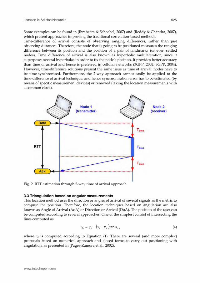
3.2 Ranging based on time measurements Considering the number of solutions currently proposed, time-based ranging seems to be a more appealing technology than solutions based on signal strength. This is because, compared to signal strength, time measurements tend to be more stable and less sensitive to environmental conditions. Time-based ranging solutions can be classified into two groups according to the number of signals/paths under consideration: time of arrival and time-difference of arrival. The former is based on estimating the distance between two nodes. It is achieved by marking transmission (ttx) and reception (trx) times and then applying txrx ttcd · (3) to compute the distance, where c stands for the propagation time (usually the speed of light). Equation (3) can only be applied if timestamps are taken under the same time line, i.e., when all nodes in the network are time-synchronised. However, this is not the normal case. Thus, the 2-way time-of-arrival approach was proposed to overcome this issue. This approach computes the propagation time under a round-trip-time approach, i.e., measuring the time spent by the signal in travelling the forward (Node 1 to Node 2) and backward (Node 2 to Node 1) paths. Fig. 2 illustrates this procedure, which is explained in detail in (Ciurana et al., 2007). Since all timestamps are taken using the same clock (in Node 1), propagation time (Tprop) can be computed as half the time measured for both paths (RTT), as long as processing time (Tproc) is negligible (or calibrated). The position of the target node (i.e., the one to be located) can be computed by multilateration once enough measurements are achieved (e.g., 3 or more for 2D positioning). The accuracy of time of arrival directly depends on the precision of the time estimations. Accordingly, there are several works addressing improvements in the accuracy of time of arrival observables.

www.intechopen.com


Some examples can be found in (Ibraheem & Schoebel, 2007) and (Reddy & Chandra, 2007), which present approaches improving the traditional correlation-based methods. Time-difference of arrival consists of observing ranging differences, rather than just observing distances. Therefore, the node that is going to be positioned measures the ranging difference between its position and the position of a pair of landmarks (or even settled nodes). Time difference of arrival is also known as hyperbolic multilateration, since it superposes several hyperbolas in order to fix the node’s position. It provides better accuracy than time of arrival and hence is preferred in cellular networks (3GPP, 2002; 3GPP, 2004). However, time-difference solutions present the same issue as time of arrival: nodes have to be time-synchronised. Furthermore, the 2-way approach cannot easily be applied to the time-difference of arrival technique, and hence synchronisation error has to be estimated (by means of specific measurement devices) or removed (taking the location measurements with a common clock).

Fig. 2. RTT estimation through 2-way time of arrival approach

3.3 Triangulation based on angular measurements This location method uses the direction or angles of arrival of several signals as the metric to compute the position. Therefore, the location techniques based on angulation are also known as Angle of Arrival (AoA) or Direction or Arrival (DoA). The position of the user can be computed according to several approaches. One of the simplest consist of intersecting the lines computed as

kjkijki xxyy tan , (4)

where αk is computed according to Equation (1). There are several (and more complex) proposals based on numerical approach and closed forms to carry out positioning with angulation, as presented in (Pages-Zamora et al., 2002).

www.intechopen.com


4. Location algorithms

Local positioning has been widely addressed for cellular networks, and the main methods and procedures remain valid for ad hoc networks. Hence, positioning algorithms draw the greatest amount of interest from the research community for location in ad hoc networks. 4.1 Taxonomy of location algorithms in ad hoc networks

4.1.1 Centralised vs. Distributed Centralised algorithms rely on a network entity (e.g., location server) that gathers the location information from all the unknown nodes and then computes their position. The main advantage is that global optimisation can be performed, as the information of all nodes is available in the location server. Centralised systems are often used in cellular networks such as public land mobile networks (PLMNs), but they collide with the random nature of ad hoc networks. The location server has to be significantly more powerful than regular nodes. Moreover, the data gathered by the server must be synchronised: all measurements must be performed at specific times. If synchronisation is not assured, optimality cannot be reached, and the system may be degraded. Additionally, topology in such systems can be displayed as a tree, with the root at the location server. Therefore, nodes near the server quickly run out their batteries, since they concentrate most of the location traffic coming from unknown nodes; this reduces the ad hoc network lifetime. In distributed location algorithms, some or all nodes are able to compute their position (and the position of other nodes depending on the specific algorithm). Thus, distributed location is more robust to node failures. Distributed algorithms also converge faster than centric solutions after topology changes and are usually insensitive to data synchronisation requirements, since only local or regional data are accounted for. There are several degrees of distributed algorithms. The most common are the localised or pure distributed algorithms, where all unknown nodes are able to compute their position once the necessary local metrics are available. 4.1.2 Incremental vs. concurrent Incremental positioning algorithms start with only a few beacon nodes. Then, in each step, the position of a reduced amount of unknown nodes is computed using the information provided by settled and beacon nodes. The positions of such nodes are used in subsequent iterations to compute the location of other unknown nodes. The advantage of iterative algorithms is their simplicity. However, they tend to propagate their positioning error, since they use metrics obtained from settled nodes for subsequent local positioning. Furthermore, the convergence of incremental location algorithms is not always guaranteed. In concurrent algorithms, all nodes are able to compute their position normally using local information. Accordingly, they are more complex than iterative algorithms, but they can avoid error propagation and hence achieve better accuracy results. 4.1.3 One hop vs. multi-hop Location involves exchanging information to measure the metrics used to compute the node’s position. One hop algorithms use only information (i.e., metrics) local to the unknown nodes (e.g., ranging to the node’s neighbours). On the other hand, multi-hop algorithms use

www.intechopen.com


information of all nodes that can be reached from the node in a certain number of hops, usually two. Muti-hop techniques allow more accurate positions to be computed and fewer beacon nodes to be deployed in the system (Savvides et al., 2001). The main drawbacks are the overhead generated by the multi-hop estimation and the subsequent use of additional resources in the nodes to store such data. 4.1.4 Beacon-Based, Mobile Beacon-Based and Beacon-Less Ad hoc location algorithms can be classified according to the presence of beacon nodes in three categories: localisation with beacons, localisation with moving beacons, and localisation without beacons (Sun et al., 2005). Localisation-with-beacons algorithms are those in which a percentage of nodes are fixed beacons, i.e., beacons that do not change their location. The major challenge of algorithms that rely on beacons is to maximise the accuracy and coverage while at the same time minimising the number of landmarks in the network. Localisation with moving beacons algorithms are similar to algorithms based on beacons, but here the beacons are no longer fixed and move through the network. A moving beacon is perceived by unknown nodes as different beacons (i.e., one per message exchanged, from different positions of the mobile beacon). Fewer landmarks are necessary, and more accurate positions can be achieved since beacon density is perceived as higher than it actually is. The main drawback with mobile beacon algorithms is that mobile beacons have to cover the entire ad hoc network and ensure that unknown nodes see the mobile beacons with a suitable frequency, which is often difficult to achieve. The last category, known as beacon-free location, involves those algorithms in which no node is aware of its position (i.e., all nodes are unknown). Thus, all nodes work together to compute their position using only their local information. This kind of algorithm usually works with a local coordinate system, which may require translation of the achieved positions into a global coordinate system so that they can be used by a location-based service or protocol. 4.1.5 Range-free vs. range-based In range-based algorithms, the local position is computed according to ranging measurements (i.e., distance or angle estimates). Accordingly, they involve multilateration techniques, which are usually hardware-demanding and therefore energy-consuming. Accordingly, range-based algorithms are suitable for ad hoc networks with powerful terminals (e.g., in technologies such as IEEE 802.11). On the other hand, technologies with more constrained terminals, such as those present in wireless sensor networks, favour the use of range-free algorithms for positioning. Range-free algorithms do not rely on ranging to compute the position of unknown nodes; rather, they consist of simpler approaches based on proximity. 4.2 State of the art The first location solutions proposed for ad hoc networks used centralised algorithms similar to techniques proposed for mobile networks. In (Doherty et al., 2001), the authors propose to manage the location as a convex-optimisation problem: a mobile server is defined to gather all the location data (e.g., distances, angles of arrival, etc.) from unknown nodes in order to compute their positions. The advantage is the simplicity and optimality of the positions computed. However, it involves delivering a significant amount of data to a location server that must be powerful enough to handle complex data structures. Moreover, the cost of the algorithm proposed for this technique is cubic in the number of connections,

www.intechopen.com


which seriously constrains the scalability of the approach. In order to overcome those drawbacks, distributed algorithms are present in many solutions. The centroid algorithm (Bulusu et al., 2000) is a one-hop pure-distributed positioning algorithm in which few beacons are spread in the ad hoc network forming a grid. Unknown nodes compute their position by estimating their range to the three closest beacons and a trilateration algorithm. The main benefit is that it is insensitive to the node density and does not add significant overhead in the network. The main drawback of this method is a larger error in the positioning. Another interesting example of a one-hop algorithm is proposed in the Lighthouse project (Römer, 2003), in which a single base station sees all sensors in the network. This full coverage is achieved by means of a beam that rotates at known speed. Stations are able to compute their position knowing the rotation speed, the width of the beam, and the signal time-of-flight. Although the accuracy might not be suitable for many applications in ad hoc networks (it provides a bias up to 14 metres), it represents an improvement in scalability. Recent proposals emphasise distributed behaviour. The Ad hoc Localisation System (AhLOS) presented in (Savvides et al., 2001) is an example of this trend. AhLOS is a one-hop pure-distributed algorithm that uses three trilateration algorithms: atomic, iterative, and collaborative. Atomic trilateration involves a one-hop scenario, where the nodes have three or more beacons in sight so that they can compute their positions directly. The main drawback of this approach is that it relies on a high density of beacons. Iterative trilateration relaxes this assumption, considering all the nodes that compute their position by means of atomic trilateration (i.e., settled nodes) as new beacons. It allows fewer beacons at the cost of less accuracy. Despite covering most of the situations, these two trilateration approaches are not sufficient to position all the nodes in the ad hoc network, since unknown nodes with only one neighbour cannot be positioned. The authors of AhLOS followed a collaborative multilateration approach to overcome this situation, consisting of identifying those unknown nodes that cannot be handled by atomic and iterative algorithms and creating groups that collaborate in order to compute the position of those nodes. This may involve solving large nonlinear systems depending on the size of the groups created. The Ad hoc Positioning System (APS) presented in (Niculescu & Nath, 2003) combines two concepts: beacon-based positioning and ad hoc propagation (i.e., multi-hop). The algorithm proposed in APS consists of four stages. Firstly, some beacon nodes are spread by the network. Secondly, nodes with some landmarks in sight measure their distance to the beacon nodes in terms of some metric, such as propagation time, number of hops, etc. Then, the information gathered by nodes in the neighbourhood of landmarks is propagated (and updated) using a proper algorithm. Finally, once a node has the ranging information of three or more beacons, it computes its position using a multilateration approach. The algorithms for propagating the ranging information in the ad hoc network are the main contribution of (Niculescu & Nath, 2003): DV-Hop, DV-distance, Euclidean, and DV-Coordinate. In the first, all nodes build ranging tables containing the position coordinates and the distance in hops to the landmarks. These data are flooded in the network in a controlled way, so that all nodes know how far they are from landmarks. On the other hand, landmarks use such data to compute the average distance of one hop, according to the hops and the distance between them. This is achieved by:

ij j

ij jiji

i h

yyxxc

22

, (5)

www.intechopen.com


where ci indicates the hop distance calculated by the landmark i, (x,y,z) are the coordinates of a landmark and hj stands for the amount of hops from landmark i to j. This average (i.e., ci) is then flooded in the network using a singleton approach: once a node receives an announcement packet from a landmark containing the average value computed by such a landmark, it discards any other further announcement packet. The average distance is then stored in the nodes, which then use it to turn distances in hops into real ranges. Finally, nodes compute their position using a multilateration approach. The advantage of this approach is that it is insensitive to the ranging error, since ranging is based on hop counting. However, it introduces more overhead than other algorithms. Moreover, accuracy is degraded in non-dense networks. The DV-distance approach is similar to DV-Hop but exchanges real distances instead of distances in hops. Multi-hop distances are computed as the sum of the distances between nodes involved in the path. Thus, this approach becomes more sensitive to ranging error. Normally, the denser the ad hoc network is, the better the accuracy. On the other hand, it improves the consistency of the DV-Hop approach, working similarly in isotropic and non-isotropic networks. The Euclidean approach involves a multi-hop algorithm, which gathers ranging information up to 2 hops. Thus, the algorithm generates quadrilaterals involving one unknown node, two neighbours, and a landmark, and it infers the distance from the node to the landmark using trigonometric formulation. The advantage of this approach is that the ranging error can be estimated, stored, and subsequently flooded together with the distance; this allows distance-weighted approaches to be used and hence more accurate positions to be achieved. The main drawback is that a 2-hop approach involves additional traffic in the network (even more than in DV-Hop and DV-Distance algorithms) as well as more resources needed in the node to store the additional information, resulting in more quickly depleting node batteries running. The last approach presented in (Niculescu & Nath, 2003) is the so-called DV-Coordinate, which is similar to the solution proposed in (Capkun et al., 2001). DV-Coordinate is based on each node computing the position of its neighbourhood according to a local coordinate-system. Then in a second step, called the registration stage, nodes exchange information to build the transformation matrices, which allow coordinates of local systems to be transformed from one local system to another. A global transformation matrix is necessary to achieve global coherence. DV-Coordinate performs almost the same as Euclidean. However, this approach impacts the scalability of the location system, since it depends on the square of the nodes in the network and involves sending two pieces of data instead of just a distance. In (Niculescu & Nath, 2003/2), the authors extend DV-Coordinate and presented the Local Positioning System (LPS), which uses ranging and angle of arrival information to compute the position of unknown nodes, in a fashion similar to the DV-Coordinate. However, the LPS reduces the overhead of the DV-Coordinate systems, thus improving the scalability and updating only a reduced number of nodes each time, not the whole network. The Amorphous Localisation algorithm (Nagpal et al., 2003) is similar to APS. It consists of computing the distance from nodes to beacons in terms of hops. However, the hop-distance is calculated offline according to the node density expected in the network. Then, a multilateration approach is followed to compute the position. The main drawback of this

www.intechopen.com


algorithm is the offline stage, which seriously constrains the scalability of the algorithm in dynamic ad hoc networks. A one-hop range-based concurrent pure-distributed algorithm is proposed in (Fu et al., 2006) for networks based on DSSS, such as those based on IEEE 802.11. This algorithm is based on propagating the clock from node to node so that the nodes involved in the positioning work in a synchronised fashion. Then the ranging to neighbour nodes is estimated, and a multilateration algorithm is applied. The synchronisation is achieved by means of the pseudo-noise code used in the DSSS, and, consequently, the time-resolution achieved matches with the code duration. Accordingly, the algorithm only works if times-of-flight are much longer than the code duration, which is expected to be the usual case. The Approximation of the Point-In-Triangulation Test (APIT) is presented in (He et al., 2003) as another example of a one-hop range-based location algorithm. It is based on generating as many triangles as possible involving three beacons. Then, the APIT algorithm evaluates whether the unknown node is inside each triangle. Finally, it overlaps all the triangles, reducing the final positioning error. The authors evaluate the algorithm through simulation and conclude that this approach outperforms the centroid algorithm. Furthermore, this approach achieves accuracy figures similar to those obtained in the APS and Amorphous Localisation algorithms but requiring a lower node density and introducing less overhead. On the other hand, it requires beacons with a radio range longer than that of regular nodes. All these approaches to the ad hoc location rely on active multilateration; i.e., positioning an unknown node involves a certain amount of location traffic in order to estimate the distances to landmarks. Active location constrains the scalability of location algorithms in ad hoc networks, in which topology and mobility are inherent to the network definition. The next sections introduce a passive algorithm for location in collaborative networks (e.g., ad hoc, wireless sensor networks, etc.), which aims to boost the scalability on positioning systems.

5. Passive positioning

Recent advances in indoor positioning have led to proposals that time-of-arrival (TOA) techniques for locating users are preferable to other techniques, such as fingerprinting. Time-of-arrival solutions achieve accuracy figures that are similar to those obtained by other techniques, but they do not require additional assistance for setup and maintenance. Conversely, time-of-arrival techniques need to calculate a client’s range from at least three receivers at known positions in order to obtain a 2D position. In addition, all the signal transmitters involved in the TOA positioning system must be synchronised. Two-way TOA techniques, such as those presented in (Ciurana et al., 2007) and (Yang et al., 2008), cope with this issue by computing the range from the client (i.e., unknown node) to the base station (i.e., landmark) using a round-trip-time (RTT) procedure. Since only the client's clock is used to calculate the range, synchronisation between base stations is no longer necessary. The drawback is that more traffic is generated on the network, thus reducing the available throughput. A recent proposal on ad hoc location presented in (Martin-Escalona & Barcelo-Arroyo, 2008) extends the capabilities of time-of-arrival location techniques, allowing unknown nodes in a network to position themselves in a passive fashion, i.e., without injecting traffic into the network. The following sections explain this technique, named passive TDOA, in detail.

www.intechopen.com


5.1 Description of assisted passive-TDOA algorithm The passive-TDOA algorithm listens to the access medium for messages that can be used to compute time-difference of arrival (TDOA) figures. The only assumption of the algorithm is that the nodes operate in a collaborative network. Note that this is the case for most of the wireless local area networks, especially those based on ad hoc protocols. In this text, one more assumption is taken only for explanatory purposes: the messages used to compute TDOAs are generated by unknown nodes running a 2-way TOA technique.

Fig. 3. Operation of the passive-TDOA algorithm The performance of the positioning algorithm is described in Fig. 3, which shows a network with three anchors or landmarks (i.e., Anchor1 to Anchor3) and two regular nodes with positioning capabilities (i.e., Node1 and Node2). At a given time, Node1 begins a TOA positioning process to locate itself. Thus, Node1 sends data message (Data1) to Anchor1 at t1, which replies with an acknowledgement (Ack1), which reaches Node1 at t2. The corresponding RTT is hence calculated as t2 – t1. Note, however, that other nodes in the network also listen to all these messages, since it is a diffusion network. Thus, Node2 hears the Data1 message at t3 and the reply to that message, i.e., Ack1, at t4. Therefore, a TDOA measurement is generated as t4 – t3. The same process is followed by Node1 to range with Anchor2 and Anchor3. Based on the assumption that Node2 is only covered at Anchor1 and Anchor2, Node2 is able to calculate two TDOAs: t4 – t3 and t7 – t6. These two measurements are enough to position Node2 using a multilateration TDOA algorithm. Note that the TDOA position calculated at Node2 involves hearing just two access points, which makes it possible

www.intechopen.com


for positioning to take place where TOA techniques would be ineffective. The only datum needed by MS2 in addition to the TDOA measurements is the position of Node1. This information can be supplied by the unknown node once it becomes settled (e.g., by broadcasting), or it can be estimated in the passive-TDOA node. Simulation analysis demonstrates that, under line-of-sight (i.e., visibility between nodes), the positioning error achieved by this algorithm is often below 1.4 times the error achieved by the 2-way TOA. Better results are achieved if the technique is deployed under non-line-of-sight conditions, providing figures similar to those achieved by the 2-way TOA technique (Martin-Escalona & Barcelo-Arroyo, 2008). This behaviour is especially relevant for location since non-line-of-sight is the usual condition for location-system operation; hence, the best performance is desired in such scenarios.

5.2 Autonomous passive TDOA: TOA position estimated One of the most constraining requirements of the passive-TDOA algorithm is the position of the 2-way TOA node. Supplying this information in location procedures where position has been requested by a third party should not involve additional changes in the 2-way TOA algorithm and could be considered the final step for the passive-TDOA algorithm. However, the same does not apply to services in which the user requests his or her own position. Although the impact of supplying the 2-way TOA positions on the capacity of the network is expected to be small, it does become necessary to define a protocol that guarantees the supply of TOA positions once they have been computed, so that passive-TDOA nodes can figure out their own locations. This protocol could involve some modifications in the 2-way TOA algorithm, which is not a desirable fact. OMA SUPL (OMA, 2008) can be used for such purposes, but security issues need to be addressed before its implementation (e.g., positions should not identify users). The algorithm initially proposed for passive-TDOA has been modified to cope with TOA position supplying. Accordingly, two operational modes have been defined: assisted and autonomous. The former consists of the algorithm as defined in the previous sections. The autonomous operational mode allows positions of TOA and passive-TDOA nodes to be jointly-computed in the passive-TDOA node, in a passive fashion. There are several benefits to computing the TOA and passive-TDOA positions jointly. The first one is that the passive-TDOA algorithm does not depend on supplying the TOA position. Accordingly, any 2-way TOA algorithm could be used together with the passive-TDOA algorithm with only slight changes. Furthermore, the passive-TDOA nodes will compute their own position and the position of the 2-way TOA nodes, which gives way to approaches for improving accuracy. The autonomous passive-TDOA algorithm becomes especially interesting in scenarios in which an application needs to locate all the users in the network. Nodes report their positions, as well as the positions of 2-way TOA nodes estimated in the passive-TDOA nodes, and then the application can use the redundancy of positions to improve the accuracy of the 2-way TOA nodes. The Autonomous mode of the passive-TDOA algorithm is based on a usual feature of 2-way TOA algorithms: the redundancy on RTTs. These algorithms tend to measure several RTTs involving the same landmark in order to reduce errors caused by the measurement system and radio channel, hence improving the accuracy. Autonomous mode uses two consecutive RTTs on the same landmark to estimate two TDOAs (as defined in the case of the normal operational mode), as well as the RTT being measured at the TOA node. As expected, the

www.intechopen.com


RTT estimate in the passive-TDOA node will be noisier than the ones made in the TOA node, but it is expected to be accurate enough to allow the passive-TDOA algorithm to compute its own position. Fig. 4 shows the procedure that constitutes the autonomous operational mode of the passive-TDOA algorithm. The explanation is based on the scenario proposed in Fig. 3, but reduced to one 2-way TOA node (i.e., Node1), a landmark (i.e., Landmark), and a passive-TDOA node (i.e., Node2). As explained for the case of the assisted operational mode, Node1 starts a ping-fashion procedure to compute the range between the landmark and itself. As a result, the RTT1 (i.e., t2 – t1) is measured. Consequently, TDOA1 is deducted from the ping procedure as t4 – t3. Until this point, the procedure is exactly the same as that presented in the case of assisted mode.

Fig. 4. Flow diagram for the autonomous operational mode of passive-TDOA algorithm Then, it is assumed that Node1 starts a new 2-way TOA procedure involving the same entities (i.e., Landmark and Node2) after a predefined time (τ), which is known by all nodes in the network. This new procedure provides new estimates for Node1 and Node2, i.e., RTT2 and TDOA2, respectively. Furthermore, autonomous mode benefits from this redundancy in the measurements by using it to estimate the ranging between Landmark and Node1 in Node2. This can be done by simply measuring a new time-difference in Node2: TDOA’. This time-difference corresponds to the difference between the arrival time to Node2 of the first TOA response and the second TOA request messages, subtracting the time elapsed between the two ping processes (i.e., t7 – t4 – τ in Fig. 4), which is assumed to be known by all nodes in the network. This information, together with the TDOA1 and TDOA2 measurements, allows the

www.intechopen.com


network to deduce the ranging information concerning Node2 and the Landmark. The formulation starts from kiRkjRjiRjiT ,,,, , (6) which computes the TDOA from the ranging information. R in Equation (6) computes the distance between two nodes, T stands for the distance-difference, and subscripts i, j, k stand for the TOA node, the landmark, and the passive-TDOA node, respectively (as in the rest of the document). According to Equation (6) and the scenario presented in Fig. 4, two TDOAs are computed as 1111 ,,,, kiRkjRjiRjiT (7) and 2222 ,,,, kiRkjRjiRjiT , (8) where the superscript indicates the ping procedure involved in the measurement. These two TDOAs (in distance) are then averaged (under the assumption of providing the same QoS) as

22 ,,21, jiTjiTjiT . (9)

According to its definition, TDOA’ is computed as 121 ,,,,' kjRkiRjiRijTTDOA . (10) Under the assumption of noiseless measurements, TOA ranging can be estimated in the passive-TDOA node as

ijTjiTjiR ,,21, . (11)

Finally, once R<i,j> is estimated, the same algorithm as used in the assisted mode is used to compute the position of the passive-TDOA node. Simulation results indicate that estimating the ranging of the 2-way TOA node results in less accurate positions, as expected. However, under non-line-of-sight conditions, which are the usual case, passive-TDOA provides positions with only 20% more error than the 2-way TOA, with the benefit of no traffic injection. This is especially relevant for group location, i.e., those applications that involve more than a single location process.

5.3 Applications of the passive-TDOA algorithm The passive-TDOA algorithm has multiple applications in the field of location. The main one has been discussed above and consists of allowing an unknown node to be positioned without injecting traffic into the network. Therefore, the load due to positioning is reduced, and the network throughput remains available for other services. This feature is essential for location algorithms since it improves scalability, which is especially essential for the location platform in the ad hoc environment.

www.intechopen.com


Another application of passive TDOA is the capability of the algorithm to position unknown nodes in environments where TOA techniques cannot. For instance, Fig. 3 shows how passive-TDOA is able to position a customer who only has two access points in sight. Under the same conditions, the TOA technique is not able to provide a location, since this technique requires at least three transmitters (even more depending on the algorithm) to perform a 2D trilateration. The passive-TDOA algorithm would be able to go further in positioning under constrained scenarios. In fact, this technique would be able to compute the position of a station with just one access point in sight, whenever enough settled nodes are in sight and their positions are known. This makes the passive-TDOA algorithm a very interesting solution for positioning under extreme conditions (e.g., scenarios in which there is interference), eventually mitigating the impact of some access points being down (e.g., due to maintenance, fire damage, etc.). Since passive-TDOA can work with fewer landmarks, it helps the system continue to offer location-based services in those circumstances where TOA is not able to provide some positions. Passive-TDOA can also be used to improve the accuracy of TOA positions. The passive-TDOA node is able to estimate its position and the positions of other TOA nodes involved as long as enough measurements are available. Subsequently, these positions can be coupled to reduce the noise and improve the final accuracy. Furthermore, this operational mode can be used to locate unknown nodes with no location capabilities at all, as explained in more detail previously in this document. All these applications of the passive-TDOA algorithm give rise to dramatic improvements in the scalability of the system, since more customers can be located while only a few TOA positioning processes are running. Note, however, that all the applications of the passive-TOA algorithm depend on their expected accuracy, since a large error in the positions computed by passive-TDOA will make these positions useless, and, therefore, system scalability will not increase at all. This work analyses the accuracy expected from passive-TDOA under several conditions and compares it with the positioning error achieved by a regular 2-way TOA algorithm. It must be noted that, even though the algorithms are addressed to ad hoc networks, they can be implemented in other networks based on infrastructure, such as those operating under the standard IEEE 802.11. In these networks, the anchors would be the access points, and the terminal nodes would be the 802.11 clients. This demonstrates the capabilities of the algorithm presented and the wide range of applications for which it can be used.

6. Conclusion

This chapter presents the positioning problem in the ad hoc context. According to the current literature, ad hoc algorithms are predominantly focused on this topic, since location techniques used for other cellular technologies remain valid in the ad hoc environment. The main algorithms proposed for ad hoc positioning are presented, giving special attention to the passive-TDOA. This algorithm is proposed to improve the scalability of 2-way TOA solutions and while at the same time providing good accuracy figures. Two operational modes are explained in detail, and the main applications for this algorithm are discussed.

www.intechopen.com


7. References

Stojmenovic, I. (2002). Position-based routing in ad hoc networks, IEEE Communications Magazine, vol. 40, July 2002, pp. 128-134, ISSN: 0163-6804.

Bourkerche, A.; Oliveira, H.; Nakamura, E. & Loureiro, A. (2007). Localization Systems for Wireless Sensor Networks, IEEE Wireless Communications, Vol. 14, December 2007, pp. 6-12, ISSN: 1536-1284.

Seidel, S.Y. & Rapport, T.S. (1992). 914 MHz path loss prediction Model for Indoor Wireless Communications in Multi-floored buildings. IEEE Trans. on Antennas & Propagation, vol. 40, no. 2, February 1992, pp. 207-217, ISSN: 0018-926X.

Wang, Y.; Jia, X. & Lee, H.K. (2003). An Indoors Wireless Positioning System Based on Wireless Local Area Network Infrastructure, Proceedings of the 6th International Symposium on Satellite Navigation, pp. 1-13, University of New South Wales, Melbourne (Australia), July 2003.

Lassabe, F.; Canalda, P.; Chatonnay, P. & Spies, F. (2005). A Friis-based calibrated model for WiFi terminals positioning, Proceedings of 6th IEEE International Symposium on a World of Wireless Mobile and Multimedia Networks (WOWMOM), pp. 382-387, ISBN: 0-7695-2342-0, Giardini Naxos, Messina (Italy), June 2005.

Bahl, P. & Padmanabhan, V. (2000). Radar: An In-Building RF-based User Location and Tracking System, Proceedings of the 19th IEEE Conference on Computer Communications (INFOCOM), vol. 2, pp. 775-784, ISBN: 0-7803-5880-5, Tel Aviv (Israel), March 2000.

Kotanen, A.; Hannikainen, M.; Leppakoski, H. & Hamalainen, T.D. (2003). Positioning with IEEE 802.11b wireless LAN. Proceedings of the 14th IEEE International Sympossium on Personal, Indoor and Mobile Radio Communications (PIMRC), vol. 3, pp. 2218-2222, ISBN: 0-7803-7822-9, Beijing (China), September 2003.

Ciurana, M.; Barcelo-Arroyo F. & Izquierdo, F. (2007). A ranging system with IEEE 802.11 data frames, Proceedings of the 1st IEEE Radio and Wireless Symposium, pp. 133-136, ISBN: 1-4244-0445-2, Long Beach, California (USA), January 2007.

Ibraheem, A. & Schoebel, J. (2007). Time of Arrival Prediction for WLAN Systems Using Prony Algorithm, Proceedings of the 4th Workshop on Positioning, Navigation and Communication (WPNC), pp. 29-32, ISBN: 1-4244-0871-7, Hannover (Germany), March 2007.

Reddy, H. & Chandra, G. (2007). An improved Time-of-Arrival estimation for WLAN-based local positioning, Proceedings of the 2nd International Conference on Communication Systems software and middleware (COMSWARE), pp. 1-5, ISBN: 1-4244-0613-7, Bangalore (India), January 2007.

3GPP. (2004). Functional stage 2 description of LCS; Technical Specification Group Services and System Aspects, 3GPP TS 23.271, version 6.8.0, June 2004.

3GPP. (2002). Location Services (LCS); Functional description; Stage 2, 3GPP TS 03.71, version 8.7.0, September 2002.

Pages-Zamora, A., Vidal, J. & Brooks, D.H. (2002). Closed-form solution for positioning based on angle of arrival measurements. Proceedings of the 13th IEEE International Symposium on Personal, Indoor and Mobile Radio Communications (PIMRC), vol. 4, pp. 1522-1526, ISBN: 0-7803-7589-0, Pavilhão Atlântico, Lisbon (Portugal), September 2002.

Savvides, A.; Han, C.C. & Srivastava, M.B. (2001). Dynamic Fine-Grained Localization in Ad-Hoc Wireless Sensor Networks. Proceedings of the 7th ACM International Conference on Mobile Computing and Networking, pp. 166-179, ISBN: 1-58113-422-3, Rome (Italy), July 2001.

www.intechopen.com


Sun, G.; Chen, J.; Guo, W. & Ray-Liu, K.J. (2005). Signal processing techniques in network-aided positioning: a survey of state-of-the-art positioning designs, IEEE Signal Processing Magazine, vol. 22, no. 4, July 2005, pp. 12-23, ISSN: 1053-5888.

Doherty, L.; Ghaoui, L.E. & Pister, K.S.J. (2001). Convex Positioning Estimation in Wireless Sensor Networks. Proceedings of the 20th IEEE Conference on Computer Communications (INFOCOM). vol. 3, pp. 1655-1663, ISBN: 0-7803-7016-3, Anchorage, AK (USA), April 2001.

Bulusu, N.; Heidemann, J. & Estrin, D. (2000). GPS-less low cost outdoor localization for very small devices, IEEE Personal Communications, vol. 7, October 2000, pp. 28-34, ISSN: 1070-9916.

Römer, K. (2003). The Lighthouse Location System for Smart Dust, Proceedings of the 1st ACM/USENIX international conference on Mobile systems, applications and services, pp. 15-30, San Francisco, California (USA), May 2003.

Niculescu, D. & Nath, B. (2003). DV based positioning in ad hoc networks. Springer Journal of Telecommunication Systems, vol. 22, no. 1-4, January 2003, pp. 267-280, ISSN: 1018-4864.

Capkun, S.; Hamdi, M. & Hubaux, J. (2001). GPS-free positioning in mobile ad-hoc networks. Proceedings of the Hawaii International Conference on Systems Sciences (HICSS), pp. 1-10, ISBN: 0-7695-0981-9, Maui, Hawaii (USA), January 2001.

Niculescu, D. & Nath, B. (2003). Localized Positioning in Ad Hoc Networks. Elsevier Ad Hoc Networks, vol. 1, no. 2-3, September 2003, pp. 247-259.

Nagpal, R.; Shrobe, H. & Bachrach, J. (2003). Organizing a Global Coordinate System from Local Information on an Ad Hoc Sensor Network. International Workshop on Information Processing in Sensor Networks (IPSN). Published as Lecture Notes in Computer Science, LNCS 2634, pp. 333-348. ISSN 0302-9743.

Fu, Y.; Liu, H.; Qin, J. & Xing, T. (2006). The localization of wireless sensor networks nodes based on DSSS. Proceedings of the IEEE International Conference on Electro/Information Technology. pp. 465-469. ISBN: 0-7803-9592-1, East Lansing, MI (USA), May 2006.

He, T.; Huang, C.; Blum, B.; Stankovic, J. & Abdelzaher, T. (2003). Range-Free Location Schemes for Large Scale Sensor Networks, Proceedings of the 9th annual international conference on Mobile computing and networking (MOBICOM), pp. 81-95, ISBN: 1-58113-753-2, San Diego, CA (USA), September 2003.

Yang, S; Kang, D.; Namgoong, Y.; Choi, S. & Shin, Y. (2008). A simple asynchronous UWB position location algorithm based on single round-trip transmission. IEICE Transactions on Fundamentals of Electronics, Communications and Computer Sciences. vol. E91-A, no. 1, January 2008, pp. 430-432, ISSN:0916-8508.

Martin-Escalona, I. & Barcelo-Arroyo, F. (2008). A New Time-Based Algorithm for Positioning Mobile Terminals in Wireless Networks, EURASIP Journal on Advances in Signal Processing, Hindawi Publishing Corporation, vol. 2008, pp. 1-10. ISSN: 1687-6172.

OMA (2008), Secure User Plane Location Architecture (SUPL), Open Mobile Alliance, [Online], http://www.openmobilealliance.org.

www.intechopen.com


www.intechopen.com

Radio CommunicationsEdited by Alessandro Bazzi

ISBN 978-953-307-091-9Hard cover, 712 pagesPublisher InTechPublished online 01, April, 2010Published in print edition April, 2010

InTech EuropeUniversity Campus STeP Ri Slavka Krautzeka 83/A 51000 Rijeka, Croatia Phone: +385 (51) 770 447 Fax: +385 (51) 686 166www.intechopen.com

InTech ChinaUnit 405, Office Block, Hotel Equatorial Shanghai No.65, Yan An Road (West), Shanghai, 200040, China

Phone: +86-21-62489820 Fax: +86-21-62489821

In the last decades the restless evolution of information and communication technologies (ICT) brought to adeep transformation of our habits. The growth of the Internet and the advances in hardware and softwareimplementations modified our way to communicate and to share information. In this book, an overview of themajor issues faced today by researchers in the field of radio communications is given through 35 high qualitychapters written by specialists working in universities and research centers all over the world. Various aspectswill be deeply discussed: channel modeling, beamforming, multiple antennas, cooperative networks,opportunistic scheduling, advanced admission control, handover management, systems performanceassessment, routing issues in mobility conditions, localization, web security. Advanced techniques for the radioresource management will be discussed both in single and multiple radio technologies; either in infrastructure,mesh or ad hoc networks.

How to referenceIn order to correctly reference this scholarly work, feel free to copy and paste the following:

Israel Martin-Escalona, Marc Ciurana and Francisco Barcelo-Arroyo (2010). Location in Ad Hoc Networks,Radio Communications, Alessandro Bazzi (Ed.), ISBN: 978-953-307-091-9, InTech, Available from:http://www.intechopen.com/books/radio-communications/location-in-ad-hoc-networks

© 2010 The Author(s). Licensee IntechOpen. This chapter is distributedunder the terms of the Creative Commons Attribution-NonCommercial-ShareAlike-3.0 License, which permits use, distribution and reproduction fornon-commercial purposes, provided the original is properly cited andderivative works building on this content are distributed under the samelicense.

https://creativecommons.org/licenses/by-nc-sa/3.0/

location in ad hoc networks

Documents