Logic and Computation

Brigitte Pientka

School of Computer ScienceMcGill UniversityMontreal, Canada

These course notes have been developed by Prof. B. Pientka for COMP527:Logic and Computation.Part of the material is based on course notes by Prof. F. Pfenning (Carnegie Mellon University). DONOT DISTRIBUTE OUTSIDE THIS CLASS WITHOUT EXPLICIT PERMISSION. Instructor generatedcourse materials (e.g., handouts, notes, summaries, homeworks, exam questions, etc.) are pro-tected by law and may not be copied or distributed in any form or in any medium without explicitpermission of the instructor. Note that infringements of copyright can be subject to follow up bythe University under the Code of Student Conduct and Disciplinary Procedures.

Copyright 2014 Brigitte Pientka

Contents

1 Introduction 5

2 Natural Deduction 72.1 Propositions . . . . . . . . . . . . . . . . . . . . . . . . . . . . . . . . . 82.2 Judgements and Meaning . . . . . . . . . . . . . . . . . . . . . . . . . 82.3 Hypothetical judgements and derivations . . . . . . . . . . . . . . . . . 102.4 Local soundness and completeness . . . . . . . . . . . . . . . . . . . . 15

2.4.1 Conjunction . . . . . . . . . . . . . . . . . . . . . . . . . . . . . 152.4.2 Implications . . . . . . . . . . . . . . . . . . . . . . . . . . . . . 162.4.3 Disjunction . . . . . . . . . . . . . . . . . . . . . . . . . . . . . 172.4.4 Negation . . . . . . . . . . . . . . . . . . . . . . . . . . . . . . 18

2.5 First-order Logic . . . . . . . . . . . . . . . . . . . . . . . . . . . . . . 192.5.1 Universal and Existential Quantification . . . . . . . . . . . . . 20

2.6 Localizing Hypothesis . . . . . . . . . . . . . . . . . . . . . . . . . . . 252.7 Proofs by structural induction . . . . . . . . . . . . . . . . . . . . . . . 272.8 Exercises . . . . . . . . . . . . . . . . . . . . . . . . . . . . . . . . . . . 28

3 Proof terms 313.1 Propositions as Types . . . . . . . . . . . . . . . . . . . . . . . . . . . . 313.2 Proving = Programming . . . . . . . . . . . . . . . . . . . . . . . . . . 383.3 Proof terms for first-order logic . . . . . . . . . . . . . . . . . . . . . . 383.4 Meta-theoretic properties . . . . . . . . . . . . . . . . . . . . . . . . . 39

3.4.1 Subject reduction . . . . . . . . . . . . . . . . . . . . . . . . . . 413.4.2 Type Uniqueness . . . . . . . . . . . . . . . . . . . . . . . . . . 41

4 Induction 434.1 Domain: natural numbers . . . . . . . . . . . . . . . . . . . . . . . . . 43

4.1.1 Defining for natural numbers . . . . . . . . . . . . . . . . . . . 444.1.2 Reasoning about natural numbers . . . . . . . . . . . . . . . . . 44

3

4.1.3 Proof terms . . . . . . . . . . . . . . . . . . . . . . . . . . . . . 454.2 Domain: Lists . . . . . . . . . . . . . . . . . . . . . . . . . . . . . . . . 484.3 Extending the induction principle to reasoning about indexed lists and

other predicates . . . . . . . . . . . . . . . . . . . . . . . . . . . . . . . 494.4 First-order Logic with Domain-specific Induction . . . . . . . . . . . . 54

5 Sequent Calculus 555.1 Normal Natural Deductions . . . . . . . . . . . . . . . . . . . . . . . . 56

5.1.1 Sequent calculus . . . . . . . . . . . . . . . . . . . . . . . . . . 625.1.2 Theoretical properties of sequent calculus . . . . . . . . . . . . 645.1.3 Cut-elimination . . . . . . . . . . . . . . . . . . . . . . . . . . . 69

5.2 Consequences of Cut Elimination . . . . . . . . . . . . . . . . . . . . . 735.3 Towards a focused sequent calculus . . . . . . . . . . . . . . . . . . . . 74

6 Normalization 816.1 General idea . . . . . . . . . . . . . . . . . . . . . . . . . . . . . . . . 826.2 Defining strongly normalizing terms . . . . . . . . . . . . . . . . . . . 826.3 Reducibility Candidates . . . . . . . . . . . . . . . . . . . . . . . . . . 856.4 Proving strong normalization . . . . . . . . . . . . . . . . . . . . . . . 866.5 Extension: Disjoint sums . . . . . . . . . . . . . . . . . . . . . . . . . . 88

6.5.1 Semantic type [[A+ B]] is a reducibility candidate . . . . . . . . 896.5.2 Revisiting the fundamental lemma . . . . . . . . . . . . . . . . 90

6.6 Extension: Recursion . . . . . . . . . . . . . . . . . . . . . . . . . . . . 916.7 Extension: Natural numbers . . . . . . . . . . . . . . . . . . . . . . . . 92

6.7.1 Semantic type [[nat]] . . . . . . . . . . . . . . . . . . . . . . . . 936.7.2 Semantic type [[nat]] is a reducibility candidate . . . . . . . . . . 936.7.3 Revisiting the fundamental lemma . . . . . . . . . . . . . . . . 94

Chapter 1

Introduction

Logic provides computer science with both a unifying foundational framework and atool for modelling. In fact, logic has been called ”the calculus of computer science”,playing a crucial role in diverse areas such as artificial intelligence, computationalcomplexity, distributed computing, database systems, hardware design, program-ming languages, and software engineering

These notes are designed to provide to give a thorough introduction to modernconstructive logic, its numerous applications in computer science, and its mathemati-cal properties. In particular, we provide an introduction to its proof-theoretic founda-tions and roots. Following Gentzen’s approach we define the meaning of propositionsby introduction rules, which assert a given proposition and explain how to concludea given proposition, and elimination rules, which justify how we can use a givenproposition and what consequences we can derive from it. In proof-theory, we areinterested in studying the structure of proofs which are constructed according to ax-ioms and inference rules of the logical system. This is in contrast to model theory,which is semantic in nature.

From a programming languages point of view, understanding the proof-theoreticfoundations is particularly fascinating because of the intimate deep connection be-tween propositions and proofs and types and programs which is often referred to asthe Curry-Howard isomorphism and establishes that proofs are isomorphic to pro-grams. This correspondence has wide-ranging consequences in programming lan-guages: it provides insights into compiler and program transformations; it forms thebasis of modern type theory and directly is exploited in modern proof assistants suchas Coq or Agda or Beluga where propositions are types and proofs correspond towell-typed programs; meta-theoretic proof techniques which have been developedfor studying proof systems are often used to establish properties and provide new in-sights about programs and programming languages (for example, type preservation

5

or normalization).These lecture notes provide an introduction to Gentzen’s natural deduction sys-

tem and its correspondance to the lambda-calculus. We will also study meta-theoreticproperties of both the natural deduction system and the well-typed lambda-calculusand highlight the symmetry behind introduction and elimination rules in logic andprogramming languages. Starting from intuitionistic propositional logic, we extendthese ideas to first-order logic and discuss how to add induction over a given domain.This gives rise to a simple dependently typed language (i.e. indexed types) over agiven domain. Finally, we will study consistency of our logic. There are two dualapproaches: the first, pursued by Gentzen, concentrates on studying the structure ofproofs; we establish consistency of the natural deduction system by translating it toa sequent calculus using cut-rule; subsequently we prove that the cut-rule is admis-sible. As a consequence, every natural deduction proof also has a cut-free proof (i.e.normal proof). However, the sequent calculus is interesting in its own since we canfurther study the structure of proofs and gain insights into how to eliminate furtherredundancy in proofs leading to focused sequent calculi which have been for exampleused to provide a type-theoretic foundation for pattern matching and different eval-uation strategies. The second approach show consistency concentrates on studyingthe structure of programs and we prove that every program normalizes using logicalrelations following Tait. This is a more direct proof than the syntactic cut-eliminationproof which relies on proof translations.

Chapter 2

Natural Deduction

“Ich wollte nun zunachst einmal einen Formalismus aufstellen, der demwirklichen Schließen moglichst nahe kommt. So ergab sich ein “Kalkuldes naturliche Schließens”.

Untersuchungen uber das logische Schließen [Gentzen(1935)]

In this chapter, we explore the fundamental principles of defining logics by revis-iting Gentzen’s system NJ [Gentzen(1935)], the calculus of natural deduction. Thecalculus was designed and developed by Gentzen to capture mathematical reasoningpractice; his calculus stands in contrast to the common systems of logic at that timeproposed by Frege, Russel, and Hilbert all of which have few reasoning reasoningprinciples, namely modus ponens, and several axioms. In Gentzen’s system on theother hand we do not in general start from axioms to derive eventually our proposi-tion; instead, we reason from assumptions. The meaning of each logical connectiveis given by rules which introduce it into the discourse together with rules which elim-inate it, i.e. rules which tell us how to use the information described by a logicalconnective in the discourse. To put it differently, the meaning of a proposition is itsuse. An important aspect of Gentzen’s system is that the meaning (i.e. the introduc-tion and elimination rules) is defined without reference to any other connective. Thisallows for modular definition and extension of the logic, but more importantly thismodularity extends to meta-theoretic study of natural deduction and greatly simpli-fies and systematically structures proofs about the logical system. We will exploit thismodularity of logics often throughout this course as we consider many fragments andextension.

Gentzen’s work was a milestone in the development of logic and it has had wideranging influence today. In particular, it has influenced how we define programminglanguages and type systems based on the observation that proofs in natural deduc-tion are isomorphic to terms in the λ-calculus. The relationship between proofs and

7

programs was first observed by Curry for Hilbert’s system of logic; Howard subse-quently observed that proofs in natural deduction directly correspond to functionalprograms. This relationship between proofs and programs is often referred as theCurry-Howard isomorphism. In this course we will explore the intimate connectionbetween propositions and proofs on the one hand and types and programs on theother.

2.1 Propositions

There are two important ingredients in defining a logic: what are the valid propo-sitions and what is their meaning. To define valid propositions, the simplest mostfamiliar way is to define their grammar using Backus-Naur form (BNF). To beginwith we define our propositions consisting of true (>), conjunction (∧), implication(⊃), and disjunction (∨).

Propositions A,B,C ::= > | A∧ B | A ⊃ B | A∨ B

We will use A, B, C to range over propositions. The grammar only defines whenpropositions are well-formed. To define the meaning of a proposition we use a judge-ment “A true”. There are many other judgements one might think of defining: A false(to define when a proposition A is false), A possible (to define when a proposition ispossible typical in modal logics), or simply A prop (to define when a proposition A iswell-formed giving us an alternative to BNF grammars).

2.2 Judgements and Meaning

We are here concerned with defining the meaning of a proposition A by definingwhen it is true. To express the meaning of a given proposition we use inferencerules. The general form of an inference rule is

J1 . . . JnJ

name

where J1, . . . , Jn are called the premises and J is called the conclusion. We can readthe inference rule as follows: Given the premises J1, . . . , Jn, we can conclude J. Aninference rule with no premises is called an axiom. We now define the meaning ofeach connective in turn.

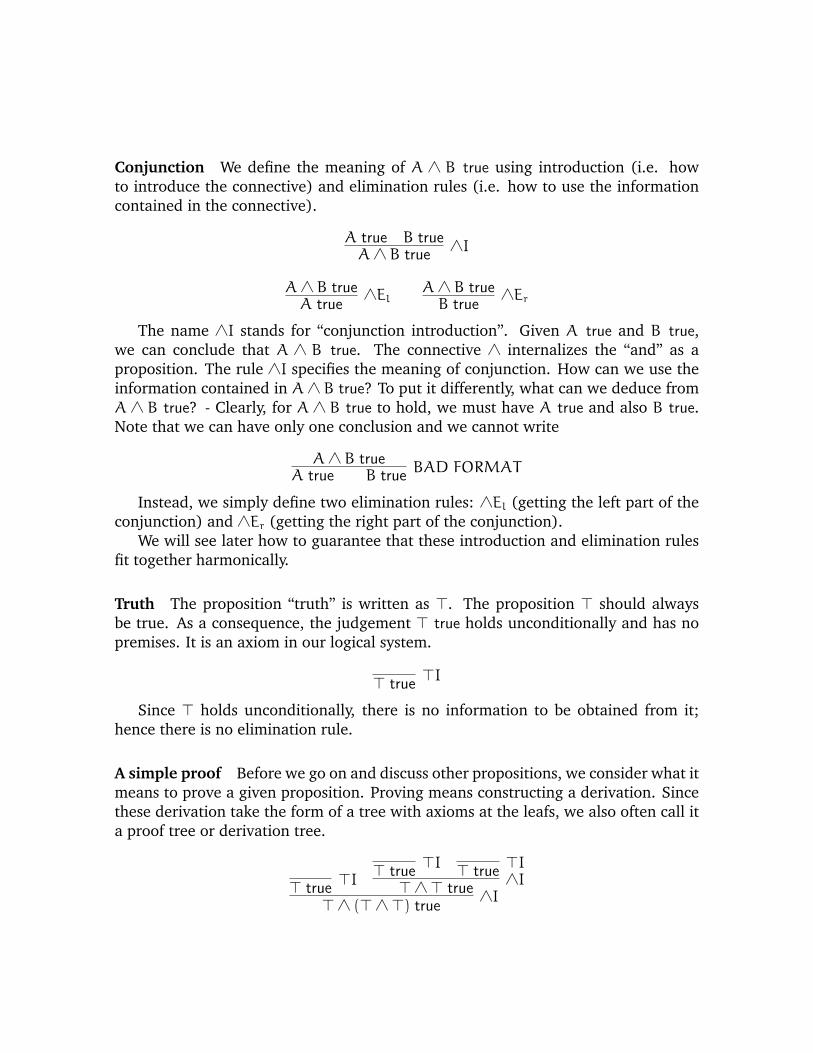
Conjunction We define the meaning of A ∧ B true using introduction (i.e. howto introduce the connective) and elimination rules (i.e. how to use the informationcontained in the connective).

A true B trueA∧ B true

∧I

A∧ B trueA true

∧ElA∧ B trueB true

∧Er

The name ∧I stands for “conjunction introduction”. Given A true and B true,we can conclude that A ∧ B true. The connective ∧ internalizes the “and” as aproposition. The rule ∧I specifies the meaning of conjunction. How can we use theinformation contained in A∧ B true? To put it differently, what can we deduce fromA ∧ B true? - Clearly, for A ∧ B true to hold, we must have A true and also B true.Note that we can have only one conclusion and we cannot write

A∧ B trueA true B true

BAD FORMAT

Instead, we simply define two elimination rules: ∧El (getting the left part of theconjunction) and ∧Er (getting the right part of the conjunction).

We will see later how to guarantee that these introduction and elimination rulesfit together harmonically.

Truth The proposition “truth” is written as >. The proposition > should alwaysbe true. As a consequence, the judgement > true holds unconditionally and has nopremises. It is an axiom in our logical system.

> true>I

Since > holds unconditionally, there is no information to be obtained from it;hence there is no elimination rule.

A simple proof Before we go on and discuss other propositions, we consider what itmeans to prove a given proposition. Proving means constructing a derivation. Sincethese derivation take the form of a tree with axioms at the leafs, we also often call ita proof tree or derivation tree.

> true>I > true

>I > true>I

>∧> true∧I

>∧ (>∧>) true∧I

Derivations convince us of the truth of a proposition. As we will see, we distin-guish between proof and derivation following philosophical ideas by Martin Lofs. Aproof, in contrast to a derivation, contains all the data necessary for computational(i.e. mechanical) verification of a proposition.

2.3 Hypothetical judgements and derivations

So far, we cannot prove interesting statements. In particular, we cannot accept as avalid derivation

A∧ (B∧ C) true

B∧ C true∧r

B true∧l

While the use of the rule ∧l and ∧r is correct, A ∧ (B ∧ C) true is unjustified.It is certainly not true unconditionally. However, we might want to say that we canderive B true, given the assumption A ∧ (B ∧ C) true. This leads us to the importantnotion of a hypothetical derivation and hypothetical judgement. In general, we mayhave more than one assumption, so a hypothetical derivation has the form

J1 . . . Jn...J

We can derive J given the assumptions J1, . . ., Jn. Note, that we make no claims asto whether we can in fact prove J1, . . ., Jn; they are unproven assumptions. However,if we do have derivations establishing that Ji is true, then we can replace the use ofthe assumption Ji with the corresponding derivation tree and eliminate the use ofthis assumption. This is called the substitution principle for hypothesis.

Implications Using a hypothetical judgement, we can now explain the meaning ofA ⊃ B (i.e. A implies B) which internalizes hypothetical reasoning on the level ofpropositions.

We introduce A ⊃ B true, if we have established A true under the assumptionB true.

A trueu

...B true

A ⊃ B true⊃ Iu

The label u indicates the assumption A true; using the label as part of the name⊃ Iu makes it clear that the assumption u can only be used to establish B true, but it isdischarged in the conclusion A ⊃ B true; we internalized it as part of the propositionA ⊃ B and the assumption A true is no longer available. Hence, assumptions existonly within a certain scope.

Many mistakes in building proofs are made by violating the scope, i.e. usingassumptions where they are not available. Let us illustrate using the rule ⊃ I in aconcrete example.

A trueu

B truev

A∧ B true∧I

B ⊃ (A∧ B) true⊃ Iv

A ⊃ B ⊃ (A∧ B) true⊃ Iu

Note implications are right associative and we do not write parenthesis aroundB ⊃ (A ∧ B). Also observe how we discharge all assumptions. It is critical that alllabels denoting assumptions are distinct, even if they denote the “same” assumption.Consider for example the following proof below.

A trueu

A truev

A∧A true∧I

A ⊃ (A∧A) true⊃ Iv

A ⊃ A ⊃ (A∧A) true⊃ Iu

We introduce A true twice giving each assumption a distinct label. There are infact many proofs we could have given for A ⊃ A ⊃ (A∧A). Some variations we givebelow.

A trueu

A truev

A∧A true∧I

A ⊃ (A∧A) true⊃ Iv

A ⊃ A ⊃ (A∧A) true⊃ Iu

A trueu

A trueu

A∧A true∧I

A ⊃ (A∧A) true⊃ Iv

A ⊃ A ⊃ (A∧A) true⊃ Iu

A truevA true

v

A∧A true∧I

A ⊃ (A∧A) true⊃ Iv

A ⊃ A ⊃ (A∧A) true⊃ Iu

The rightmost derivation does not use the assumption u while the middle deriva-tion does not use the assumption v. This is fine; assumptions do not have to be used

and additional assumptions do not alter the truth of a given statement. Moreover, wenote that both trees use an assumption more than once; this is also fine. Assumptionscan be use as often as we want to. Finally, we note that the order in which assump-tions are introduced does not enforce order of use, i.e. just because we introducethe assumption u before v, we are not required to first use u and then use v. Theorder of assumptions is irrelevant. We will make these structural properties aboutassumptions more precise when we study the meta-theoretic properties of our logicalsystem.

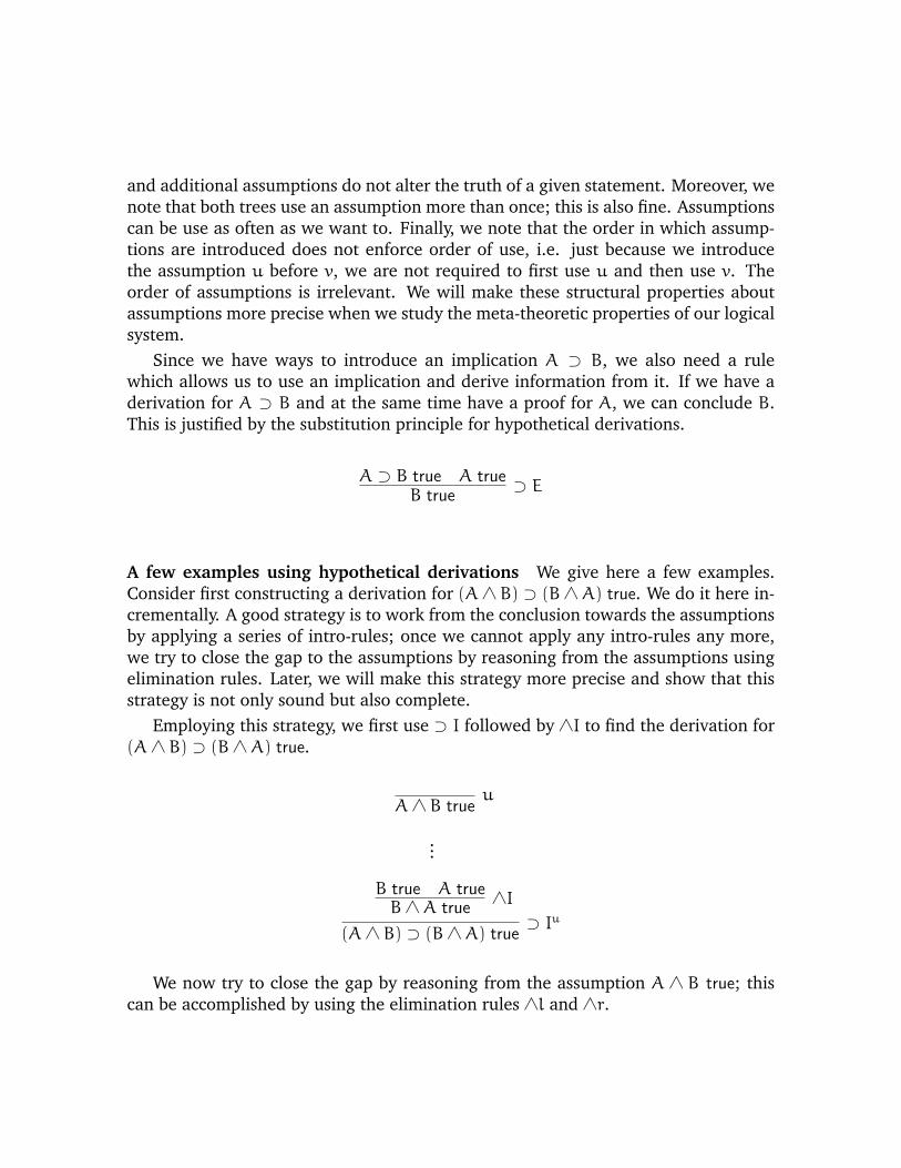
Since we have ways to introduce an implication A ⊃ B, we also need a rulewhich allows us to use an implication and derive information from it. If we have aderivation for A ⊃ B and at the same time have a proof for A, we can conclude B.This is justified by the substitution principle for hypothetical derivations.

A ⊃ B true A trueB true

⊃ E

A few examples using hypothetical derivations We give here a few examples.Consider first constructing a derivation for (A∧ B) ⊃ (B∧A) true. We do it here in-crementally. A good strategy is to work from the conclusion towards the assumptionsby applying a series of intro-rules; once we cannot apply any intro-rules any more,we try to close the gap to the assumptions by reasoning from the assumptions usingelimination rules. Later, we will make this strategy more precise and show that thisstrategy is not only sound but also complete.

Employing this strategy, we first use ⊃ I followed by ∧I to find the derivation for(A∧ B) ⊃ (B∧A) true.

A∧ B trueu

...

B true A trueB∧A true

∧I

(A∧ B) ⊃ (B∧A) true⊃ Iu

We now try to close the gap by reasoning from the assumption A ∧ B true; thiscan be accomplished by using the elimination rules ∧l and ∧r.

A∧ B trueu

B true∧Er

A∧ B trueu

A true∧El

B∧A true∧I

(A∧ B) ⊃ (B∧A) true⊃ Iu

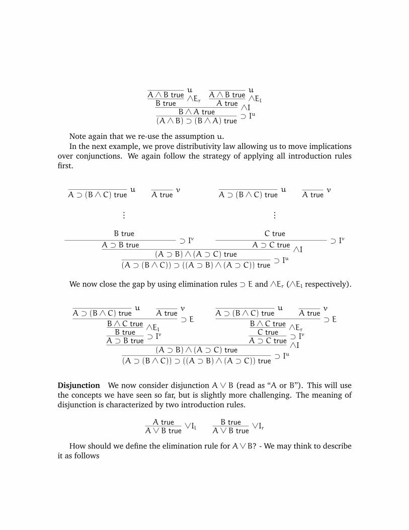
Note again that we re-use the assumption u.In the next example, we prove distributivity law allowing us to move implications

over conjunctions. We again follow the strategy of applying all introduction rulesfirst.

A ⊃ (B∧ C) trueu

A truev

...

B true

A ⊃ B true⊃ Iv

A ⊃ (B∧ C) trueu

A truev

...

C true

A ⊃ C true⊃ Iv

(A ⊃ B)∧ (A ⊃ C) true∧I

(A ⊃ (B∧ C)) ⊃ ((A ⊃ B)∧ (A ⊃ C)) true⊃ Iu

We now close the gap by using elimination rules ⊃ E and ∧Er (∧El respectively).

A ⊃ (B∧ C) trueu

A truev

B∧ C true⊃ E

B true∧El

A ⊃ B true⊃ Iv

A ⊃ (B∧ C) trueu

A truev

B∧ C true⊃ E

C true∧Er

A ⊃ C true⊃ Iv

(A ⊃ B)∧ (A ⊃ C) true∧I

(A ⊃ (B∧ C)) ⊃ ((A ⊃ B)∧ (A ⊃ C)) true⊃ Iu

Disjunction We now consider disjunction A ∨ B (read as “A or B”). This will usethe concepts we have seen so far, but is slightly more challenging. The meaning ofdisjunction is characterized by two introduction rules.

A trueA∨ B true

∨IlB true

A∨ B true∨Ir

How should we define the elimination rule for A∨B? - We may think to describeit as follows

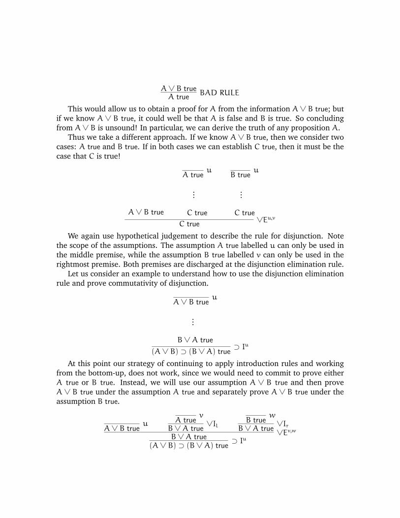
A∨ B trueA true

BAD RULE

This would allow us to obtain a proof for A from the information A∨ B true; butif we know A ∨ B true, it could well be that A is false and B is true. So concludingfrom A∨ B is unsound! In particular, we can derive the truth of any proposition A.

Thus we take a different approach. If we know A∨ B true, then we consider twocases: A true and B true. If in both cases we can establish C true, then it must be thecase that C is true!

A∨ B true

A trueu

...

C true

B trueu

...

C true

C true∨Eu,v

We again use hypothetical judgement to describe the rule for disjunction. Notethe scope of the assumptions. The assumption A true labelled u can only be used inthe middle premise, while the assumption B true labelled v can only be used in therightmost premise. Both premises are discharged at the disjunction elimination rule.

Let us consider an example to understand how to use the disjunction eliminationrule and prove commutativity of disjunction.

A∨ B trueu

...

B∨A true

(A∨ B) ⊃ (B∨A) true⊃ Iu

At this point our strategy of continuing to apply introduction rules and workingfrom the bottom-up, does not work, since we would need to commit to prove eitherA true or B true. Instead, we will use our assumption A ∨ B true and then proveA ∨ B true under the assumption A true and separately prove A ∨ B true under theassumption B true.

A∨ B trueu A true

v

B∨A true∨Il

B truew

B∨A true∨Ir

B∨A true∨Ev,w

(A∨ B) ⊃ (B∨A) true⊃ Iu

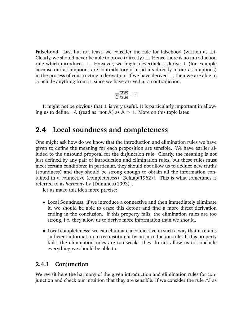
Falsehood Last but not least, we consider the rule for falsehood (written as ⊥).Clearly, we should never be able to prove (directly) ⊥. Hence there is no introductionrule which introduces ⊥. However, we might nevertheless derive ⊥ (for examplebecause our assumptions are contradictory or it occurs directly in our assumptions)in the process of constructing a derivation. If we have derived ⊥, then we are able toconclude anything from it, since we have arrived at a contradiction.

⊥ trueC true

⊥E

It might not be obvious that ⊥ is very useful. It is particularly important in allow-ing us to define ¬A (read as “not A) as A ⊃ ⊥. More on this topic later.

2.4 Local soundness and completeness

One might ask how do we know that the introduction and elimination rules we havegiven to define the meaning for each proposition are sensible. We have earlier al-luded to the unsound proposal for the disjunction rule. Clearly, the meaning is notjust defined by any pair of introduction and elimination rules, but these rules mustmeet certain conditions; in particular, they should not allow us to deduce new truths(soundness) and they should be strong enough to obtain all the information con-tained in a connective (completeness) [Belnap(1962)]. This is what sometimes isreferred to as harmony by [Dummett(1993)].

let us make this idea more precise:

• Local Soundness: if we introduce a connective and then immediately eliminateit, we should be able to erase this detour and find a more direct derivationending in the conclusion. If this property fails, the elimination rules are toostrong, i.e. they allow us to derive more information than we should.

• Local completeness: we can eliminate a connective in such a way that it retainssufficient information to reconstitute it by an introduction rule. If this propertyfails, the elimination rules are too weak: they do not allow us to concludeeverything we should be able to.

2.4.1 Conjunction

We revisit here the harmony of the given introduction and elimination rules for con-junction and check our intuition that they are sensible. If we consider the rule ∧I as

a complete definition for A ∧ B true, we should be able to recover both A true andB true.

Local soundnessD1

A trueD2B true

∧IA∧ B true

∧ElA true =⇒ D1

A true

and symmetrically

D1A true

D2B true

∧IA∧ B true

∧ElA true =⇒ D2

B true

Clearly, it is unnecessary to first introduce a conjunction and then immediatelyeliminate it, since there is a more direct proof already. These detours are what makesproof search infeasible in practice in the natural deduction calculus. It also meansthat there are many different proofs for a give proposition many of which can collapseto the more direct proof which does not use the given detour. This process is callednormalization - or trying to find a normal form of a proof.

Local completeness We need to show that A∧B true contains enough informationto rebuild a proof for A∧ B true.

DA∧ B true

=⇒

DA∧ B true

∧ElA true

DA∧ B true

∧ErB true

∧IA∧ B true

2.4.2 Implications

Next, we revisit the given introduction and elimination rules for implications. Again,we first verify that we can introduceA ⊃ B followed by eliminating it without gainingadditional information.

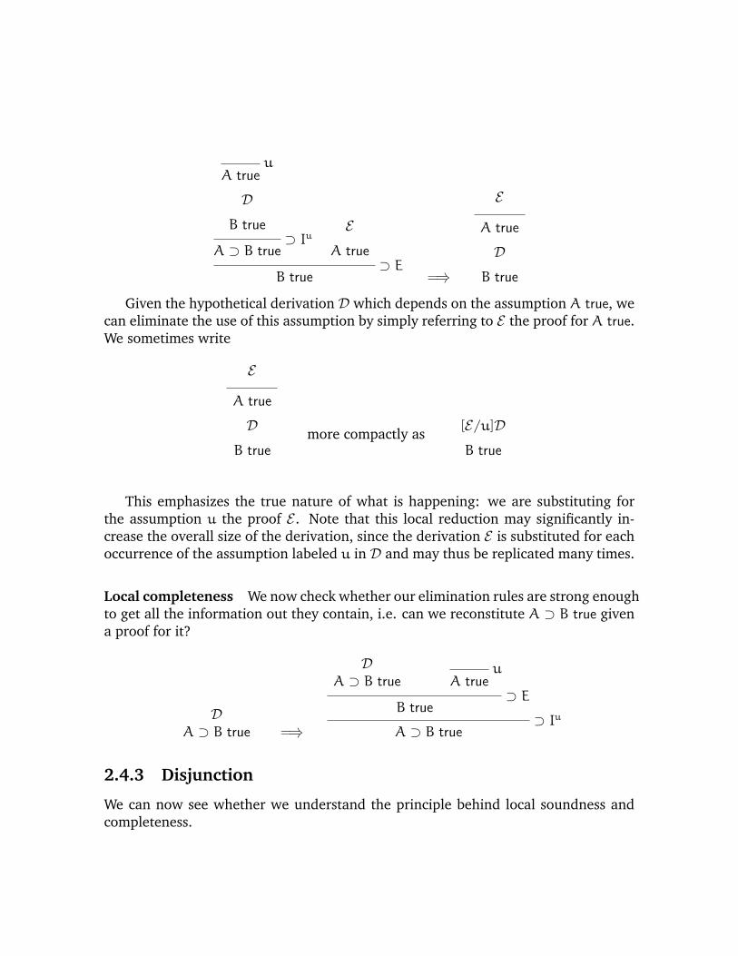
uA true

D

B true⊃ Iu

A ⊃ B true

E

A true⊃ E

B true =⇒

E

A true

D

B true

Given the hypothetical derivation D which depends on the assumption A true, wecan eliminate the use of this assumption by simply referring to E the proof for A true.We sometimes write

E

A true

D

B truemore compactly as [E/u]D

B true

This emphasizes the true nature of what is happening: we are substituting forthe assumption u the proof E . Note that this local reduction may significantly in-crease the overall size of the derivation, since the derivation E is substituted for eachoccurrence of the assumption labeled u in D and may thus be replicated many times.

Local completeness We now check whether our elimination rules are strong enoughto get all the information out they contain, i.e. can we reconstitute A ⊃ B true givena proof for it?

DA ⊃ B true =⇒

DA ⊃ B true

uA true

⊃ EB true

⊃ IuA ⊃ B true

2.4.3 Disjunction

We can now see whether we understand the principle behind local soundness andcompleteness.

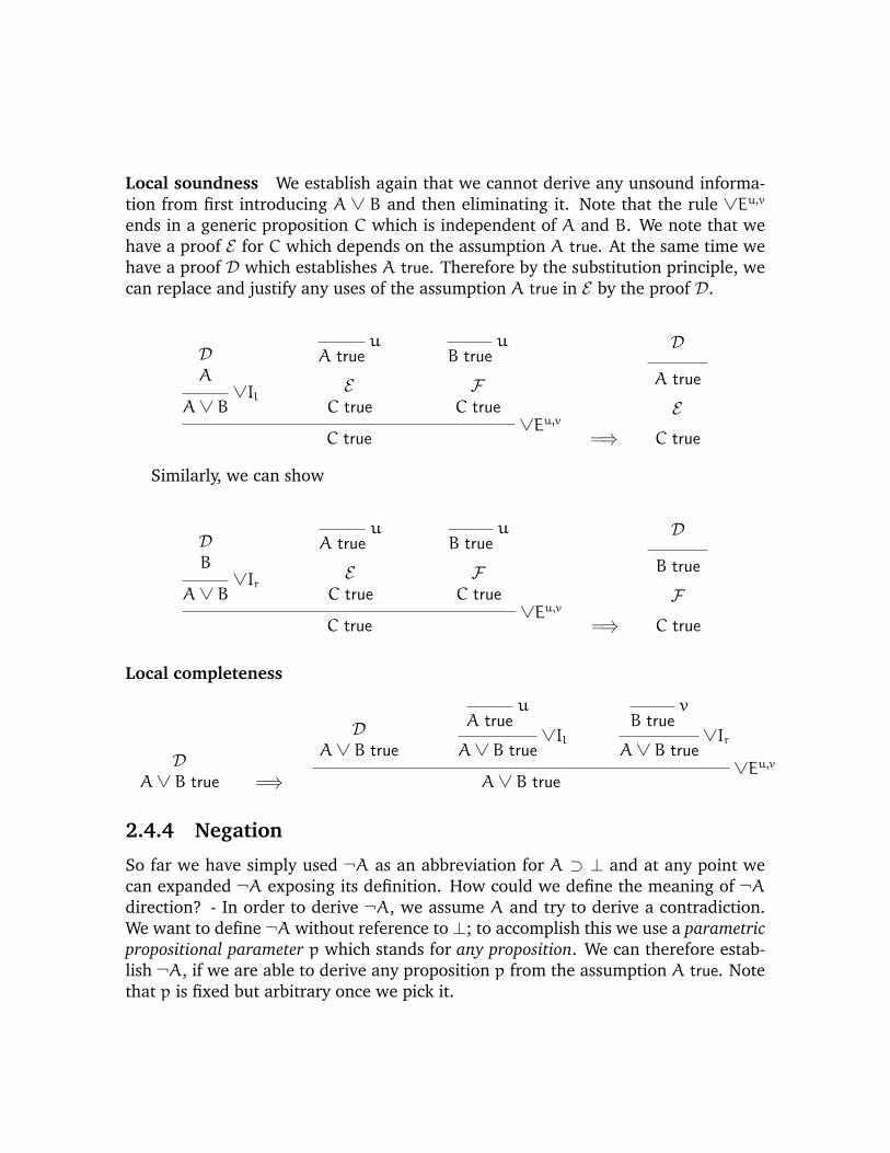
Local soundness We establish again that we cannot derive any unsound informa-tion from first introducing A ∨ B and then eliminating it. Note that the rule ∨Eu,v

ends in a generic proposition C which is independent of A and B. We note that wehave a proof E for C which depends on the assumption A true. At the same time wehave a proof D which establishes A true. Therefore by the substitution principle, wecan replace and justify any uses of the assumption A true in E by the proof D.

DA

∨IlA∨ B

uA true

EC true

uB true

FC true

∨Eu,vC true =⇒

D

A true

E

C true

Similarly, we can show

DB

∨IrA∨ B

uA true

EC true

uB true

FC true

∨Eu,vC true =⇒

D

B true

F

C true

Local completeness

DA∨ B true =⇒

DA∨ B true

uA true

∨IlA∨ B true

vB true

∨IrA∨ B true

∨Eu,vA∨ B true

2.4.4 Negation

So far we have simply used ¬A as an abbreviation for A ⊃ ⊥ and at any point wecan expanded ¬A exposing its definition. How could we define the meaning of ¬Adirection? - In order to derive ¬A, we assume A and try to derive a contradiction.We want to define ¬A without reference to ⊥; to accomplish this we use a parametricpropositional parameter p which stands for any proposition. We can therefore estab-lish ¬A, if we are able to derive any proposition p from the assumption A true. Notethat p is fixed but arbitrary once we pick it.

uA true

...p true

¬Ip,u¬A true

¬A true A true¬E

C true

We can check again local soundness: if we introduce ¬A and then eliminate it,we have not gained any information.

uA true

D

p true¬Ipu

¬A true

E

A true¬E

C true =⇒

E

A true

[C/p]D

C true

Since p denotes any proposition and D is parametric in p, we can replace p withC; moreover, since we have a proof E for A, we can also eliminate the assumption uby replacing any reference to u with the actual proof E .

The local expansion is similar to the case for implications.

D¬A true =⇒

D¬A true

uA true

⊃ Ep true

⊃ Ipu¬A true

It is important to understand the use of parameters here. Parameters allow us toprove a given judgment generically without committing to a particular proposition.As a rule of thumb, if one rule introduces a parameter and describes a derivationwhich holds generically, the other must is a derivation for a concrete instance.

2.5 First-order Logic

So far, we have considered propositional logic and the programming language arisingfrom it is very basic. It does not allow us to reason about data-types such as naturalnumbers or booleans for example.

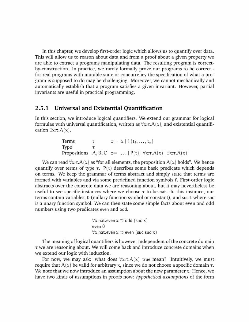
In this chapter, we develop first-order logic which allows us to quantify over data.This will allow us to reason about data and from a proof about a given property weare able to extract a programs manipulating data. The resulting program is correct-by-construction. In practice, we rarely formally prove our programs to be correct -for real programs with mutable state or concurrency the specification of what a pro-gram is supposed to do may be challenging. Moreover, we cannot mechanically andautomatically establish that a program satisfies a given invariant. However, partialinvariants are useful in practical programming.

2.5.1 Universal and Existential Quantification

In this section, we introduce logical quantifiers. We extend our grammar for logicalformulae with universal quantification, written as ∀x:τ.A(x), and existential quantifi-cation ∃x:τ.A(x).

Terms t ::= x | f (t1, . . . , tn)Type τ

Propositions A,B,C ::= . . . | P(t) | ∀x:τ.A(x) | ∃x:τ.A(x)

We can read ∀x:τ.A(x) as “for all elements, the proposition A(x) holds”. We hencequantify over terms of type τ. P(t) describes some basic predicate which dependson terms. We keep the grammar of terms abstract and simply state that terms areformed with variables and via some predefined function symbols f. First-order logicabstracts over the concrete data we are reasoning about, but it may nevertheless beuseful to see specific instances where we choose τ to be nat. In this instance, ourterms contain variables, 0 (nullary function symbol or constant), and suc t where sucis a unary function symbol. We can then state some simple facts about even and oddnumbers using two predicates even and odd.

∀x:nat.even x ⊃ odd (suc x)even 0∀x:nat.even x ⊃ even (suc suc x)

The meaning of logical quantifiers is however independent of the concrete domainτ we are reasoning about. We will come back and introduce concrete domains whenwe extend our logic with induction.

For now, we may ask: what does ∀x:τ.A(x) true mean? Intuitively, we mustrequire that A(x) be valid for arbitrary x, since we do not choose a specific domain τ.We note that we now introduce an assumption about the new parameter x. Hence, wehave two kinds of assumptions in proofs now: hypothetical assumptions of the form

A true as for example introduced by the rules ⊃ I or ∨E and parametric assumptionsof the form x:τ.

a:τ...

A(a) true∀Ia

∀x:τ.A(x) true

∀x:τ.A(x) true t:τ∀E

A(t) true

If our domain τ is finite, we might hope to check for each element ti in τ thatA(ti) true. However, our domain may be infinite which makes this approach infea-sible. Instead, we make no commitment as to what shape or property the elementmight have and pick one representative a. Note that a is arbitrary and fresh, i.e.it cannot have been used before in the same derivation. If we are able to establishA(a) true then it is indeed the case that ∀x:τ.A(x) true, because we have proven Agenerically for an arbitrary a.

If we have a proof of ∀x:τ.A(x) true, then we know that A(x) is true for arbitraryx. Hence, we should be able to obtain specific instances by instantiating x with aconcrete term of type τ. In the rule ∀E, we explicitly establish the fact that t hastype τ using the judgment t:τ. We keep the definition of t:τ abstract at this point, butkeep in mind for every concrete domain τ we can define terms belonging to it. Forexample, for the domain nat, we might define

N00 : nat

t : natNsuc

suc t : nat

We return to other domains shortly.We can now prove some simple statements which are true for any domain τ such

as the following:

u∀x:τ.P(x)∧Q(x) true a : τ

∀EP(a)∧Q(a) true

∧ElP(a) true

∀Ia∀x:τ.P(x) true

u∀x:τ.P(x)∧Q(x) true b : τ

∀EP(b)∧Q(b) true

∧ErQ(b) true

∀Ib∀x:τ.Q(x) true

∧I(∀x:τ.P(x))∧ (∀x:τ.Q(x)) true

⊃ Iu(∀x:τ.P(x)∧Q(x)) ⊃ (∀x:τ.P(x))∧ (∀x:τ.Q(x)) true

We note that the parameter a in the left branch is different from the parameterb in the right branch; we chose different names for clarity, however note since theirscope is different, choosing the same name in both branches would still be fine andthey would still refer be distinct.

To check that our introduction and elimination rules are harmonic, we give localsoundness and completeness proofs.

x:τ

D

A(x) true∀Iu

∀x:τ.A(x) true

E

t:τ∀E

A(t) true =⇒

E

t : τ

[t/x]D

A(t) true

Since the derivation D is parametric in x, we can simply replace all instances of xwith concrete terms t of the same type.

We now check whether our elimination rules are strong enough to get all theinformation out they contain, i.e. can we reconstitute ∀x:τ.A(x) true given a prooffor it?

D∀x:τ.A true =⇒

D∀x:τ.A(x) true x : τ

∀EA(x) true

∀Ix∀x:τ.A(x) true

Let us now define the meaning of existential quantification. (Finite) universalquantification corresponds to conjunction; dually, (finite) existential quantificationcorresponds to disjunction. To prove ∃x:τ.A(x), we pick a term t from τ and showA(t) true. Note that we require that t actually exists. This is an important distinctionin reasoning constructively. It means we require that the type τ is in fact inhabited,i.e. elements exist and it is not empty. Classically, we are not required to provide anelement explicitly. As a consequence, one might argue that constructive reasoningallows us to make more fine-grained distinction between when a domain is emptyand when it is not. In fact, constructively, we can interpret the empty type as falsewhich is often exploited in practice.

Our existential introduction rule is similar to disjunction in that we need to picka t belonging to τ. It involves a choice.

A(t) true t : τ∃I

∃x:τ.A(x) true

∃x:τ.A(x)

a:τu

A(a) true...

C true∃Ea,u

C true

What can we deduce given a proof for ∃x:τ.A(x)? - Although we know that thereexists some element a in τ such that A(a) true, we don’t know which one. Recallagain the elimination rule for disjunction where we had a similar dilemma. Althoughwe have A ∨ B true, we do not know whether A true or B true. We therefore splitthe proof into two cases: Assuming A true we can prove C true and assuming B truewe can prove C true. We will define existential elimination similarly; if the domainτ were finite, we would have n cases to consider: assuming A(ti) true we proveC true for all 1 ≤ i ≤ n. However, we do not make any assumptions about ourdomain. Hence, we hence pick a fresh arbitrary parameter a and assuming A(a) truewe establish C true. Since a was arbitrary and we have a proof for ∃x:τ.A(x), wehave established C true.

Let us consider an example to see how we prove statements involving existentialquantification.

(∃x:τ.P(x)∨Q(x)) ⊃ (∃x:τ.P(x))∨ (∃x:τ.Q(x)) true

We show the proof in two stages, since its proof tree is quite large.

u∃x:τ.P(x)∨Q(x) true

vP(a)∨Q(a) true a:τ

Davu(∃x:τ.P(x))∨ (∃x:τ.Q(x)) true

∃Eav(∃x:τ.P(x))∨ (∃x:τ.Q(x)) true

⊃ Iu(∃x:τ.P(x)∨Q(x)) ⊃ (∃x:τ.P(x))∨ (∃x:τ.Q(x)) true

We now give the derivation Dauv; we write the assumptions available as a super-script.

vP(a)∨Q(a) true

w1P(a) true a:τ

∃I∃x:τ.P(x) true

∨Ir(∃x:τ.P(x))∨ (∃x:τ.Q(x)) true . . .

∨Ew1w2

(∃x:τ.P(x))∨ (∃x:τ.Q(x)) true

To understand better the interaction between universal and existential quantifi-cation, let’s consider the following statement.

∃x:τ.¬A(x) ⊃ ¬∀x:τ.A(x) true

u∃x:τ.¬A(x) true

u∀x:τ.A(x) true a:τ

∀EA(a) true

v¬A(a) true

⊃ E⊥ true

∃Eav⊥ true

⊃ Iw¬∀x:τ.A(x) true

⊃ Iu∃x:τ.¬A(x) ⊃ ¬∀x:τ.A(x) true

Let’s consider the converse;

(¬∀x:τ.A(x)) ⊃ ∃x:τ.¬A(x) true

After using implication introduction, we are in the following situation:

u¬∀x:τ.A(x) true

...∃x:τ.¬A(x) true

⊃ Iu(¬∀x:τ.A(x)) ⊃ ∃x:τ.¬A(x) true

But now we are stuck; to use the rule ∃I we need a concrete witness for x, whichwe do not have, since we know nothing about the domain τ. We also cannot doanything with the assumption ¬∀x:τ.A(x) which is equivalent to ∀x:τ.A(x) ⊃ ⊥. Toeliminate it, we would need a proof of ∀x:τ.A(x).

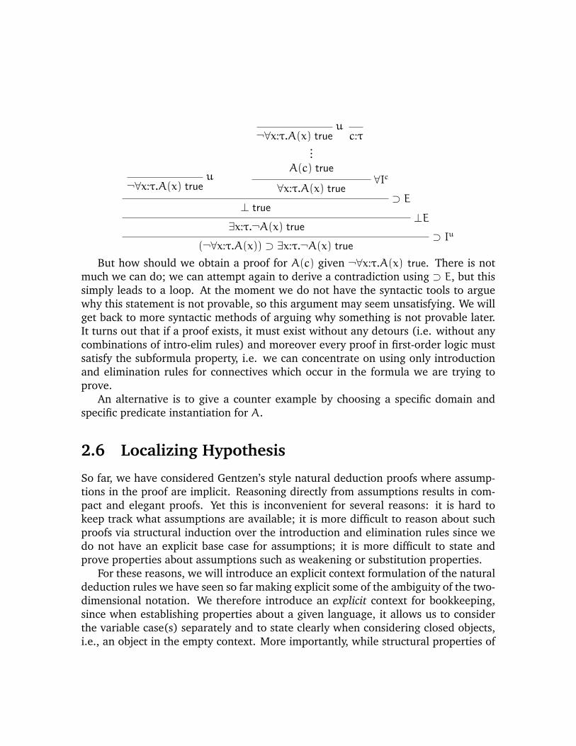
u¬∀x:τ.A(x) true

u¬∀x:τ.A(x) true c:τ

...A(c) true

∀Ic∀x:τ.A(x) true

⊃ E⊥ true

⊥E∃x:τ.¬A(x) true

⊃ Iu(¬∀x:τ.A(x)) ⊃ ∃x:τ.¬A(x) true

But how should we obtain a proof for A(c) given ¬∀x:τ.A(x) true. There is notmuch we can do; we can attempt again to derive a contradiction using ⊃ E, but thissimply leads to a loop. At the moment we do not have the syntactic tools to arguewhy this statement is not provable, so this argument may seem unsatisfying. We willget back to more syntactic methods of arguing why something is not provable later.It turns out that if a proof exists, it must exist without any detours (i.e. without anycombinations of intro-elim rules) and moreover every proof in first-order logic mustsatisfy the subformula property, i.e. we can concentrate on using only introductionand elimination rules for connectives which occur in the formula we are trying toprove.

An alternative is to give a counter example by choosing a specific domain andspecific predicate instantiation for A.

2.6 Localizing Hypothesis

So far, we have considered Gentzen’s style natural deduction proofs where assump-tions in the proof are implicit. Reasoning directly from assumptions results in com-pact and elegant proofs. Yet this is inconvenient for several reasons: it is hard tokeep track what assumptions are available; it is more difficult to reason about suchproofs via structural induction over the introduction and elimination rules since wedo not have an explicit base case for assumptions; it is more difficult to state andprove properties about assumptions such as weakening or substitution properties.

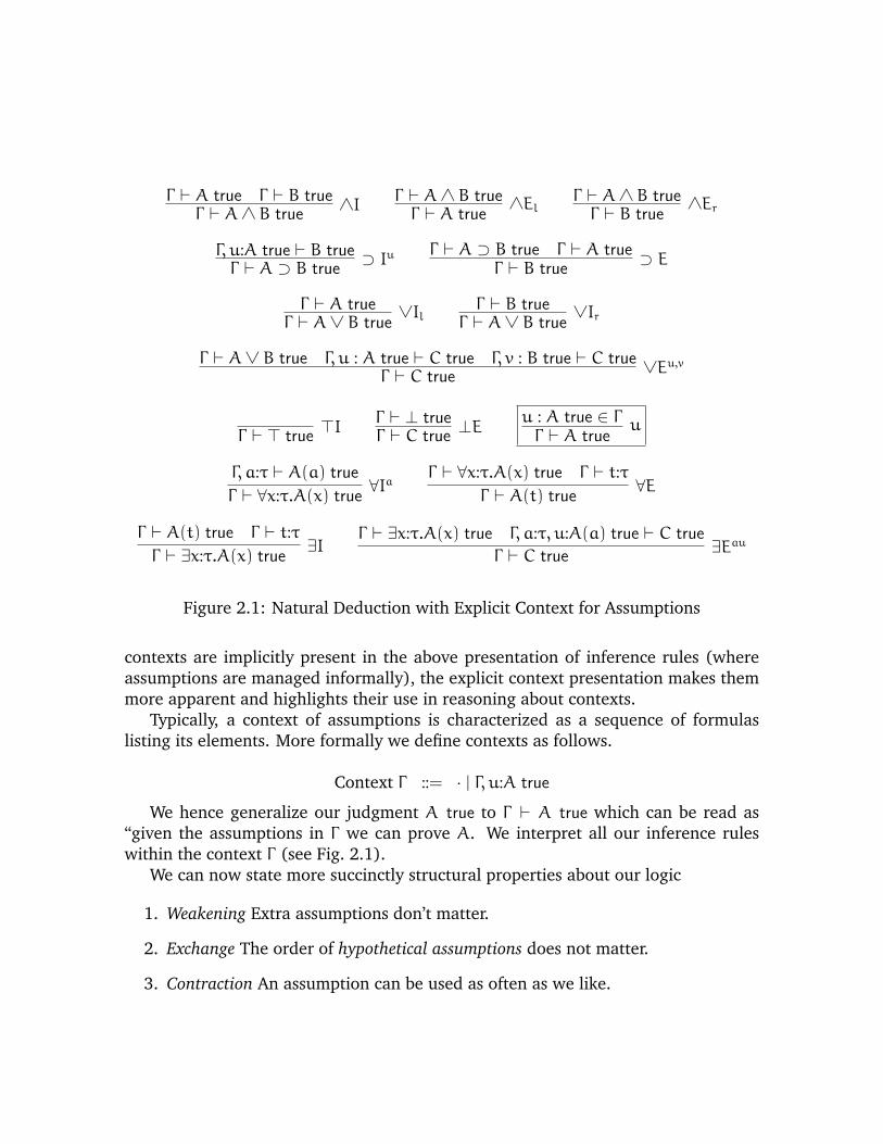
For these reasons, we will introduce an explicit context formulation of the naturaldeduction rules we have seen so far making explicit some of the ambiguity of the two-dimensional notation. We therefore introduce an explicit context for bookkeeping,since when establishing properties about a given language, it allows us to considerthe variable case(s) separately and to state clearly when considering closed objects,i.e., an object in the empty context. More importantly, while structural properties of

Γ ` A true Γ ` B trueΓ ` A∧ B true

∧IΓ ` A∧ B trueΓ ` A true

∧ElΓ ` A∧ B trueΓ ` B true

∧Er

Γ, u:A true ` B trueΓ ` A ⊃ B true

⊃ Iu Γ ` A ⊃ B true Γ ` A trueΓ ` B true

⊃ E

Γ ` A trueΓ ` A∨ B true

∨IlΓ ` B true

Γ ` A∨ B true∨Ir

Γ ` A∨ B true Γ, u : A true ` C true Γ, v : B true ` C trueΓ ` C true

∨Eu,v

Γ ` > true>I Γ ` ⊥ true

Γ ` C true⊥E u : A true ∈ Γ

Γ ` A trueu

Γ, a:τ ` A(a) true

Γ ` ∀x:τ.A(x) true∀Ia

Γ ` ∀x:τ.A(x) true Γ ` t:τΓ ` A(t) true

∀E

Γ ` A(t) true Γ ` t:τΓ ` ∃x:τ.A(x) true

∃IΓ ` ∃x:τ.A(x) true Γ, a:τ, u:A(a) true ` C true

Γ ` C true∃Eau

Figure 2.1: Natural Deduction with Explicit Context for Assumptions

contexts are implicitly present in the above presentation of inference rules (whereassumptions are managed informally), the explicit context presentation makes themmore apparent and highlights their use in reasoning about contexts.

Typically, a context of assumptions is characterized as a sequence of formulaslisting its elements. More formally we define contexts as follows.

Context Γ ::= · | Γ, u:A true

We hence generalize our judgment A true to Γ ` A true which can be read as“given the assumptions in Γ we can prove A. We interpret all our inference ruleswithin the context Γ (see Fig. 2.1).

We can now state more succinctly structural properties about our logic

1. Weakening Extra assumptions don’t matter.

2. Exchange The order of hypothetical assumptions does not matter.

3. Contraction An assumption can be used as often as we like.

as actual theorems which can be proven by structural induction.

Theorem 2.6.1.

1. Weakening. If Γ, Γ ′ ` A true then Γ, u : B true, Γ ′ ` A true.

2. Exchange If Γ, x : B1 true, y : B2 true, Γ ′ ` A truethen Γ, y : B2 true, x : B1 true, Γ ′ ` A true.

3. Contraction If Γ, x : B true, y : B true, Γ ′ ` A true then Γ, x : B true, Γ ′ ` A true.

In addition to these structural properties, we can now also state succinctly thesubstitution property.

Theorem 2.6.2 (Substitution).If Γ, x : A true, Γ ′ ` B true and Γ ` A true then Γ, Γ ′ ` B true.

2.7 Proofs by structural induction

We will here review how to prove properties about a given formal system; this is incontrast to reasoning within a given formal system. It is also referred to as “meta-reasoning”.

One of the most common meta-reasoning techniques is “proof by structural in-duction on a given proof tree or derivation”. One can always reduce this structuralinduction argument to a mathematical induction purely based on the height of theproof tree. We illustrate this proof technique by proving the substitution property.

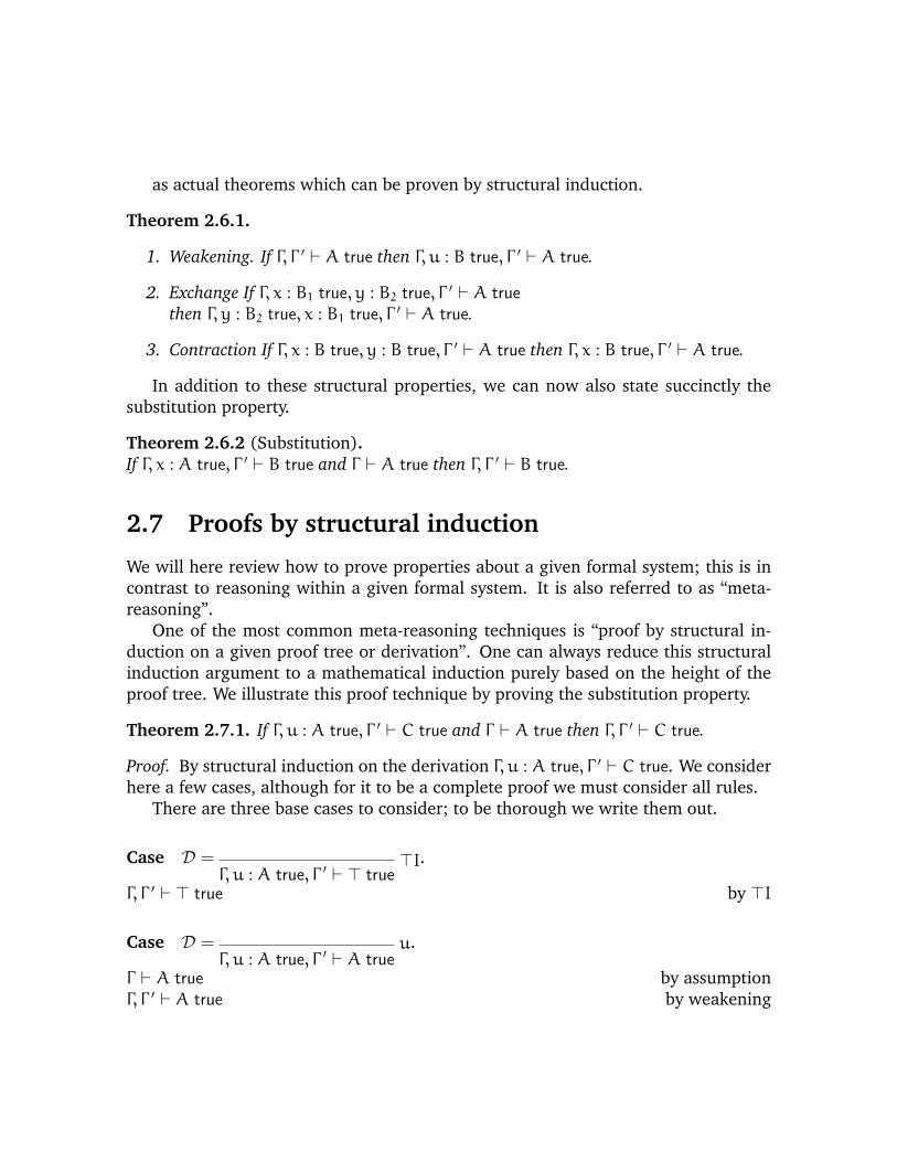
Theorem 2.7.1. If Γ, u : A true, Γ ′ ` C true and Γ ` A true then Γ, Γ ′ ` C true.

Proof. By structural induction on the derivation Γ, u : A true, Γ ′ ` C true. We considerhere a few cases, although for it to be a complete proof we must consider all rules.

There are three base cases to consider; to be thorough we write them out.

Case D = >IΓ, u : A true, Γ ′ ` > true

.

Γ, Γ ′ ` > true by >I

Case D = uΓ, u : A true, Γ ′ ` A true

.

Γ ` A true by assumptionΓ, Γ ′ ` A true by weakening

Case D =v : C true ∈ (Γ, Γ ′)

vΓ, u : A true, Γ ′ ` C true

Γ, Γ ′ ` C true by rule v

We now consider some of the step cases. The induction hypothesis allos us to assumethe substitution property holds for smaller derivations.

Case D =

F

Γ, u : A true, Γ ′ ` C true

E

Γ, u : A true, Γ ′ ` B true∧I

Γ, u : A true, Γ ′ ` C∧ B true

Γ ` A true by assumptionΓ, Γ ′ ` C true by i.h. using F and assumptionΓ, Γ ′ ` B true by i.h. using E and assumptionΓ, Γ ′ ` C∧ B true by rule ∧I

The other cases for ∧El, ∧Er, ⊃ E, ∨Il, ∨Ir, or ⊥E follow a similar schema. Abit more interesting are those cases where we introduce new assumptions and thecontext of assumptions grows.

Case D =

E

Γ, u : A true, Γ ′, v:B true ` C true⊃ Iv

Γ, u : A true, Γ ′ ` B ⊃ C true

Γ ` A true by assumptionΓ, Γ ′, v : B true ` C true by i.h. using EΓ, Γ ′ ` B ⊃ C true by rule ⊃ Iv.

Note that the appeal to the induction hypothesis is valid, because the height ofthe derivation E is smaller than the height of the derivation D. Our justification isindependent of the fact that the context in fact grew.

2.8 Exercises

Exercise 2.8.1. Assume someone defines conjunction with the following two rules:

A∧ B

uA

vB

...C

∧Eu,vC

A B∧I

A∧ B

Are these rules sound and complete? – Show local soundness and completeness.

Exercise 2.8.2. Give a direct definition of “A iff B”, which means “A implies B andB implies A”.

1. Give introduction and elimination rules for iff without recourse to any otherlogical connectives.

2. Display the local reductions that show the local soundness of the eliminationrules.

3. Display the local expansion that show the local completeness of the eliminationrules.

Exercise 2.8.3. A∧B is usually defined as ¬(A∧ B). In this problem we explore thedefinition of nand using introduction and elimination rules.

1. Give introduction and elimination rules for nand without recourse to any otherlogical connectives.

2. Display the local reductions that show the local soundness of the eliminationrules.

3. Display the local expansion that show the local completeness of the eliminationrules.

Exercise 2.8.4. Extend the proof of the substitution lemma for the elimination rulesfor conjunction (∧Ei) and disjunction (∨E).

Chapter 3

Proof terms

“For my money, Gentzens natural deduction and Churchs lambda calcu-lus are on a par with Einsteins relativity and Diracs quantum physics forelegance and insight. And the maths are a lot simpler. “

Proofs as Programs: 19th Century Logic and 21 Century Computing, P.Wadler [?]

In this chapter, we describe the relationship between propositions and proofs on theone hand and types and programs on the other. On the propositional fragment oflogic this is referred to as the Curry-Howard isomorphism. Martin Lof developed thisintimate relationship of propositions and types further leading to what we call typetheory. More precisely, we will establish the relationship between natural deductionproofs and programs written in Church’s lambda-calculus.

3.1 Propositions as Types

In order to highlight the relationship between proofs and programs, we introduce anew judgement M : A which reads as “M is a proof term for proposition A”. Ourintention is to capture the structure of the proof using M. As we will see there arealso other interpretations of this judgement:

M : AM is a proof term for proposition AM is a program of type A

These dual interpretations are at the heart of the Curry-Howard isomorphism. Wecan think ofM as the term that represents the proof of A true or we think of A as thetype of the program M.

Our intention is that

31

M : A iff A true

However, we want in fact that that the derivation for M : A has the identicalstructure as the derivation for A true. This is stronger than simply whenever M : Athen A true and vice versa. We will revisit our natural deduction rules and annotatethem with proof terms. The isomorphism betweenM : A andA true will then becomeobvious.

Conjunction Constructively, we can think of A ∧ B true as a pair of proofs: theproof M for A true and the proof N for B true.

M : A N : B∧I

〈M, N〉 : A∧ B

The elimination rules correspond to the projections from a pair to its first andsecond element.

M : A∧ B∧El

fst M : A

M : A∧ B∧Er

snd M : B

In other words, conjunction A∧ B corresponds to the cross product type A× B.We can also annotate the local soundness rule:

D1M : A

D2N : B

∧I〈M, N〉 : A∧ B

∧Elfst 〈M, N〉 : A =⇒ D1

M : A

and dually

D1M : A

D2N : B

∧I〈M, N〉 : A∧ B

∧Elsnd 〈M, N〉 : A =⇒ D2

N : B

The local soundness proofs for ∧ give rise to two reduction rule:

fst 〈M, N〉 =⇒ M

snd 〈M, N〉 =⇒ N

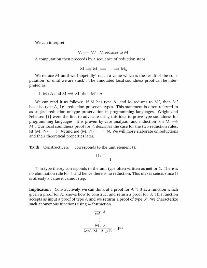
We can interpret

M =⇒M ′ M reduces to M ′

A computation then proceeds by a sequence of reduction steps:

M =⇒M1 =⇒ . . . =⇒Mn

We reduce M until we (hopefully) reach a value which is the result of the com-putation (or until we are stuck). The annotated local soundness proof can be inter-preted as:

If M : A and M =⇒M ′ then M ′ : A

We can read it as follows: If M has type A, and M reduces to M ′, then M ′

has also type A, i.e. reduction preserves types. This statement is often referred toas subject reduction or type preservation in programming languages. Wright andFelleisen [?] were the first to advocate using this idea to prove type soundness forprogramming languages. It is proven by case analysis (and induction) on M =⇒M ′. Our local soundness proof for ∧ describes the case for the two reduction rules:fst 〈M, N〉 =⇒ M and snd 〈M, N〉 =⇒ N. We will more elaborate on reductionsand their theoretical properties later.

Truth Constructively, > corresponds to the unit element ().

() : >>I

> in type theory corresponds to the unit type often written as unit or 1. There isno elimination rule for > and hence there is no reduction. This makes sense, since ()is already a value it cannot step.

Implication Constructively, we can think of a proof for A ⊃ B as a function whichgiven a proof for A, knows how to construct and return a proof for B. This functionaccepts as input a proof of type A and we returns a proof of type B”. We characterizesuch anonymous functions using λ-abstraction.

x:Au

...M : B

λx:A.M : A ⊃ B ⊃ Ix,u

We distinguish here in the derivation between the variable x corresponding to Aand the assumption which states x has type A. Here x is a proof term, while u thename of the assumption x : A. Consider the trivial proof for (A∧A) ⊃ A true.

ux : A

∧Elfst x : A

⊃x,uλx:(A∧A).fst x : (A∧A) ⊃ A

A different proof where we extract the rightA fromA∧A, can results in a differentproof term.

ux : A

∧Ersnd x : A

⊃x,uλx:(A∧A).snd x : (A∧A) ⊃ A

The probably simplest proof for A ⊃ A can be described by the identity functionλx:A.x.

The elimination rule for ⊃ E corresponds to function application. Given the proofterm M for proposition (type) A ⊃ B and a proof term N for proposition (type) A,characterize the proof term for B using the application MN.

M : A ⊃ B N : A⊃ E

M N : B

An implications A ⊃ B can be interpreted as a function type A→ B.The introduc-tion rule corresponds to the typing rule for function abstractions and the eliminationrule corresponds to the typing rule for function application.

Note that we continue to recover the natural deduction rules by simply erasingthe proof terms. This will continue to be the case and highlights the isomorphicstructure of proof trees and typing derivations.

As a second example, let us consider the proposition (A ∧ B) ⊃ (B ∧ A) whoseproof we’ve seen earlier as

∧ErA∧ B

B true

∧ElA∧ B

A true∧I

B∧A) true⊃ Iu

(A∧ B) ⊃ (B∧A) true

We now annotate the derivation with proof terms.

u∧Er

x : A∧ B

snd x : B

u∧El

x : A∧ B

fst x : A∧I

〈snd x, fst x〉 : B∧A)⊃ Iu

λx:A∧ B.〈snd x, fst x〉 : (A∧ B) ⊃ (B∧A)

Let us revisit the local soundness proof for ⊃ to highlight the interaction betweenfunction abstraction and function application.

ux : AD

M : B⊃ Ix,u

λx:A.B : A ⊃ BE

N : A⊃ E

(λx:A.M) N : B=⇒

Eu

N : A

[N/x]D

[N/x]M : B

This gives rise to the reduction rule for function applications:

(λx:A.M) N =⇒ [N/x]M

The annotated soundness proof above corresponds to the case in proving that thereduction rule preserves types. It also highlights the distinction between x whichdescribes a term of type A and u which describes the assumption that x has type A.In the proof, we appeal in fact to two substitution lemmas:

1. Substitution lemma on terms: Replace any occurrence of x with N

2. Substitution lemma on judgements: Replace the assumption N : A with a proofE which establishes N : A.

Disjunction Constructively, a proof ofA∨B says that we have either a proof ofA ora proof of B. All possible proofs of A∨ B can be described as a set containing proofsof A and proofs of B. We can tag the elements in this set depending on whether theyprove A or B. Since A occurs in the left position of ∨, we tag elements denotinga proof M of A with inlA M; dually B occurs in the right position of ∨ and we tag

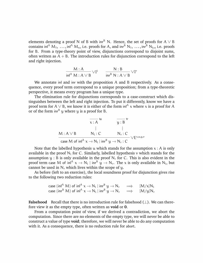
elements denoting a proof N of B with inrB N. Hence, the set of proofs for A ∨ B

contains inlA M1, . . . , inlA Mn, i.e. proofs for A, and inrB N1, . . . , inrB Nk,, i.e. proofsfor B. From a type-theory point of view, disjunctions correspond to disjoint sums,often written as A + B. The introduction rules for disjunction correspond to the leftand right injection.

M : A∨Il

inlA M : A∨ B

N : B∨Ir

inrB N : A∨ B

We annotate inl and inr with the proposition A and B respectively. As a conse-quence, every proof term correspond to a unique proposition; from a type-theoreticperspective, it means every program has a unique type.

The elimination rule for disjunctions corresponds to a case-construct which dis-tinguishes between the left and right injection. To put it differently, know we have aproof term for A∨ B, we know it is either of the form inlA x where x is a proof for Aor of the form inrB y where y is a proof for B.

M : A∨ B

ux : A

...Nl : C

vy : B

...Nr : C

∨Ex,u,y,v

case M of inlA x→ Nl | inrB y→ Nr : C

Note that the labelled hypothesis u which stands for the assumption x : A is onlyavailable in the proof Nl for C. Similarly, labelled hypothesis v which stands for theassumption y : B is only available in the proof Nr for C. This is also evident in theproof term case M of inlA x → Nl | inrB y → Nr. The x is only available in Nl, butcannot be used in Nr which lives within the scope of y.

As before (left to an exercise), the local soundness proof for disjunction gives riseto the following two reduction rules:

case (inlA M) of inlA x→ Nl | inrB y→ Nr =⇒ [M/x]Nl

case (inrB M) of inlA x→ Nl | inrB y→ Nr =⇒ [M/y]Nr

Falsehood Recall that there is no introduction rule for falsehood (⊥). We can there-fore view it as the empty type, often written as void or 0.

From a computation point of view, if we derived a contradiction, we abort thecomputation. Since there are no elements of the empty type, we will never be able toconstruct a value of type void; therefore, we will never be able to do any computationwith it. As a consequence, there is no reduction rule for abort.

M : ⊥ ⊥EabortC M : C

To guarantee that abortC M has a unique type, we annotate it with the propositionC.

Summary The previous discussion completes the proofs as programs interpretationfor propositional logic.

Propositions Types> () or 0 Unit typeA∧ B A× B Product typeA ⊃ B A→ B Function typeA∨ B A+ B Disjoint sum type⊥ void or 1 Empty type

The proof terms we introduced corresponds to the simply-typed lambda-calculuswith products, disjoint sums, unit and the empty type.

Terms M,N ::= x

| 〈M, N〉 | fst M | snd M| λx:A.M |MN

| inlA M | inrB N | case M of inlA x→ Nl | inrB y→ Nr

| abortA M | ()

Remarkably, this relationship between propositions and types can be extended toricher logics. As we will see, first-order logic gives rise to dependent types; second-order logic gives rise to polymorphism and what is generally known as the calculusSystem F. Adding fix-points to the logic corresponds to recursive data-types in pro-gramming languages. Moving on to non-classical logics such as temporal logics theircomputational interpretation provides a justification for and guarantees about re-active programming; modal logics which distinguish between truths in our currentworld and universal truths give rise to programming languages for mobile comput-ing and staged computation. The deep connection between logic, propositions andproofs on the one hand and type theory, types, and programs on the other providesa rich and fascinating framework for understanding programming languages, reduc-tion strategies, and how we reason in general.

3.2 Proving = Programming

One important consequence of the relationship between a proof and a well-typedprogram, is that instead of constructing a derivation for a proposition A, we simplywrite a program of type A. By the Curry-Howard isomorphism, this program will becorrect by construction!

As computer scientists, we are familiar with writing programs, maybe more thanwriting proof derivations. It is often also a lot more compact and less time consuming,to directly write the program corresponding to a given type A. We can then simplycheck that the program has type A, which boils down to constructing the proof treewhich establishes that A is true. The good news is that such proof checking can beeasily implemented by a small trusted type checker, a program of a few lines. In fact,Tutch gives you the option of either writing a proof for a proposition A, writing anannotated proof of a proposition A, or simply writing a term whose type is A.

We’ve already seen some simple programs, such as the identity function, or thefunction which given a pair returns the first or second projection of it. Let’s practicesome more.

Function composition The proposition ((A ⊃ B)∧ (B ⊃ C)) ⊃ A ⊃ C can be readcomputationally as function composition. Given a pair of functions, where the firstelement is a function f : A ⊃ B and the second element is a function g : B ⊃ C, wecan construct a function of type A ⊃ C, by assuming x:A, and then first feeding it tof, and passing the result of fx to g, i.e. returning a function λx:A.g (f x).

Since our language does not use pattern matching to access the first and secondelement of a pair, we write fst u instead of f and snd u instead of g, where u denotesthe assumption (A ⊃ B)∧ (B ⊃ C).

Given this reasoning, we can write function composition as

λu:(A ⊃ B)∧ (B ⊃ C).λx:A.snd u ((fst u) x)

3.3 Proof terms for first-order logic

Similar to proof terms for propositional logic, we can introduce proof terms for quan-tifiers. The proof term for introducing an existential quantifier, encapsulates the wit-ness t together with the actual proof M. It is hence similar to a pair and we writeit as 〈M, t〉 overloading the pair notation. The elimination rule for existentials ismodeled by let 〈u, a, =〉M in N where M is the proof for ∃x:τ.A(x) and N is theproof depending on the assumption u : A(a) and a : τ.

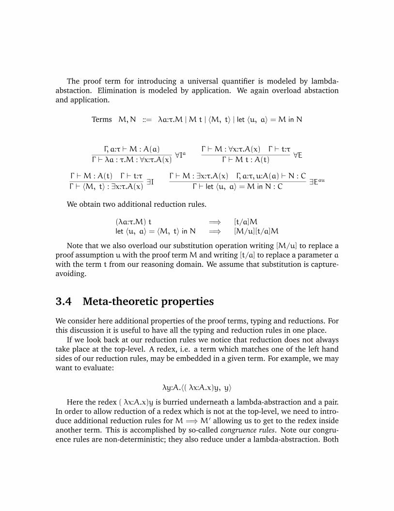
The proof term for introducing a universal quantifier is modeled by lambda-abstaction. Elimination is modeled by application. We again overload abstactionand application.

Terms M,N ::= λa:τ.M |M t | 〈M, t〉 | let 〈u, a〉 =M in N

Γ, a:τ `M : A(a)

Γ ` λa : τ.M : ∀x:τ.A(x) ∀Ia

Γ `M : ∀x:τ.A(x) Γ ` t:τΓ `M t : A(t)

∀E

Γ `M : A(t) Γ ` t:τΓ ` 〈M, t〉 : ∃x:τ.A(x) ∃I

Γ `M : ∃x:τ.A(x) Γ, a:τ, u:A(a) ` N : C

Γ ` let 〈u, a〉 =M in N : C∃Eau

We obtain two additional reduction rules.

(λa:τ.M) t =⇒ [t/a]Mlet 〈u, a〉 = 〈M, t〉 in N =⇒ [M/u][t/a]M

Note that we also overload our substitution operation writing [M/u] to replace aproof assumption u with the proof termM and writing [t/a] to replace a parameter awith the term t from our reasoning domain. We assume that substitution is capture-avoiding.

3.4 Meta-theoretic properties

We consider here additional properties of the proof terms, typing and reductions. Forthis discussion it is useful to have all the typing and reduction rules in one place.

If we look back at our reduction rules we notice that reduction does not alwaystake place at the top-level. A redex, i.e. a term which matches one of the left handsides of our reduction rules, may be embedded in a given term. For example, we maywant to evaluate:

λy:A.〈( λx:A.x)y, y〉

Here the redex ( λx:A.x)y is burried underneath a lambda-abstraction and a pair.In order to allow reduction of a redex which is not at the top-level, we need to intro-duce additional reduction rules for M =⇒M ′ allowing us to get to the redex insideanother term. This is accomplished by so-called congruence rules. Note our congru-ence rules are non-deterministic; they also reduce under a lambda-abstraction. Both

Γ `M : A Γ ` N : BΓ ` 〈M, N〉 : A∧ B

∧IΓ ` fst M : A∧ B

Γ `M : A∧El

Γ ` snd M : A∧ BΓ `M : B

∧Er

Γ, u:A `M : BΓ ` λu:A.M : A ⊃ B ⊃ I

u Γ `M : A ⊃ B Γ ` N : AΓ `MN : B

⊃ E

Γ ` N : A

Γ ` inlB N : A∨ B∨Il

Γ ` N : BΓ ` inrA N : A∨ B

∨Ir

Γ `M : A∨ B Γ, u : A ` Nl : C Γ, v : B ` Nr : C

Γ ` case M of inlu B→ Nl | inrv A→ Nr : C∨Eu,v

Γ ` () : > >IΓ ` abortC M : ⊥Γ `M : C

⊥E u : A ∈ ΓΓ ` u : A

u

Γ, a:τ `M : A(a)

Γ ` λa : τ.M : ∀x:τ.A(x) ∀Ia

Γ `M : ∀x:τ.A(x) Γ ` t:τΓ `M t : A(t)

∀E

Γ `M : A(t) Γ ` t:τΓ ` 〈M, t〉 : ∃x:τ.A(x) ∃I

Γ `M : ∃x:τ.A(x) Γ, a:τ, u:A(a) ` N : C

Γ ` let 〈u, a〉 =M in N : C∃Eau

Figure 3.1: Summary of typing rules

of these characteristics may not be wanted if we are to define a determinstic call-by-value evaluation strategy. However, at this point, we retain as much flexibility aspossible.

Exercise 3.4.1.

Define corresponding congruence rules for universal and existentials.

3.4.1 Subject reduction

We prove here a key property: Subject reduction.

Theorem 3.4.1. If M =⇒M ′ and Γ `M : C then Γ `M ′ : C.

Proof. By structural induction on M =⇒M ′.The reduction rules for each redex form the base cases in the proof. We consider

here the rule for reducing (λx:A.M) N one as an example.

Case D = (λx:A.M) N =⇒ [N/x]MΓ ` (λx:A.M) N : C by assumptionΓ ` λx:A.M : A ′ ⊃ CΓ ` N : A ′ by rule ⊃ EΓ, x : A `M : C and A = A ′ by rule ⊃ IxΓ ` [N/x]M : C by substitution lemma

We next consider a representative from the step cases which arise due to thecongruence rules.

Case D =

D ′

M =⇒M ′

λx:A.M =⇒ λx:A.M ′

Γ ` λx:A.M : C by assumptionΓ, x : A `M : B and C = A ⊃ B by rule ⊃ IxΓ, x : A `M ′ : B by i.h. on D ′Γ ` λx:A.M ′ : A ⊃ B by rule ⊃ Ix

3.4.2 Type Uniqueness

Reduction rules for redexes

fst 〈M, N〉 =⇒ M

snd 〈M, N〉 =⇒ N

(λx:A.M) N =⇒ [N/x]M

case (inlA M) of inlA x→ Nl | inrB y→ Nr =⇒ [M/x]Nl

case (inrB M) of inlA x→ Nl | inrB y→ Nr =⇒ [M/y]Nr

(λa:τ.M) t =⇒ [t/a]Mlet 〈u, a〉 = 〈M, t〉 in N =⇒ [M/u][t/a]M

Congruence rules

M =⇒M ′

〈M, N〉 =⇒ 〈M ′, N〉N =⇒ N ′

〈M, N〉 =⇒ 〈M, N ′〉 M =⇒M ′

fst M =⇒ fst M ′M =⇒M ′

snd M =⇒ snd M ′

M =⇒M ′

λx:A.M =⇒ λx:A.M ′M =⇒M ′

MN =⇒M ′ N

N =⇒ N ′

MN =⇒MN ′

M =⇒M ′

inlB M =⇒ inlB M ′

M =⇒M ′

inrA M =⇒ inrA M ′

M =⇒M ′

case M of inlB u→ Nl | inrA v→ Nr =⇒ case M ′ of inlB u→ Nl | inrA v→ Nr

Nl =⇒ N ′l

case M of inlB u→ Nl | inrA v→ Nr =⇒ case M of inlB u→ N ′l | inrA v→ Nr

Nr =⇒ N ′r

case M of inlB u→ Nl | inrA v→ Nr =⇒ case M of inlB u→ N ′l | inrA v→ N ′r

Figure 3.2: Summary of reduction rules

Chapter 4

Induction

So far, we have seen first-order logic together with its corresponding proof-terms.First-order logic corresponds to the dependently typed lambda-calculus. However, ifwe are to write meaningful programs we need two more ingredients: 1) we needto reason about specific domains such as natural numbers, lists, etc 2) we needto be able to write recursive programs about elements in a given domain. Proof-theoretically, we would like to add the power of induction which as it turns outcorresponds to being able to write total well-founded recursive programs.

4.1 Domain: natural numbers

First-order logic is independent of a given domain and the reasoning principles wedefined hold for any domain. Nevertheless, it is useful to consider specific domains.There are several approaches to incorporating domain types or index types into ourlanguage: One is to add a general definition mechanism for recursive types or induc-tive types. We do not consider this option here, but we return to this idea later. An-other one is to use the constructs we already have to define data. This was Church’soriginal approach; he encoded numerals, booleans as well as operations such as ad-dition, multiplication, if-statements, etc. as lambda-terms using a Church encoding.We will not discuss this idea in these notes. A third approach is to specify each typedirectly by giving rules defining how to construct elements of a given type (introduc-tion rule) and how to reason with elements of a given type (elimination rule). Thisis the approach we will be pursuing here.

We begin by defining concretely the judgement

t : τ Term t has type τ

43

which we have left more or less abstract for now for concrete instances of τ.

4.1.1 Defining for natural numbers

We define elements belonging to natural numbers via two constructors z and suc .They allow us to introduce natural numbers. We can view these two rules as intro-duction rules for natural numbers.

natIzz : nat

t : natnatIsuc

suc t : nat

4.1.2 Reasoning about natural numbers

To prove inductively a property A(t) true, we establish three things:

1. t is a natural number and hence we know how to split it into different cases.

2. Base case: A(z) trueEstablish the given property for the number z

3. Step case: For any n : nat, assume A(n) true (I.H) and prove A(sucn) true.We assume the property holds for smaller numbers, i.e. for n, and we establishthe property for sucn.

More formally, the inference rule capturing this idea is given below:

t : nat A(z) true

n : nati.h

A(n) true...

A(sucn) truenatEn,ih

A(t) true

Restating the rule using explicit contexts to localize all assumptions:

Γ ` t : nat Γ ` A(z) true Γ, n:nat, ih:A(n) true ` A(sucn) truenatEn,ih

Γ ` A(t) true

Let us prove a simple property inductively, to see how we use the rule.Note the rule natEn,ih has implicitly a generalization built-in. If we want to estab-

lish a property A(42) true, we may choose to prove it more generally for any number

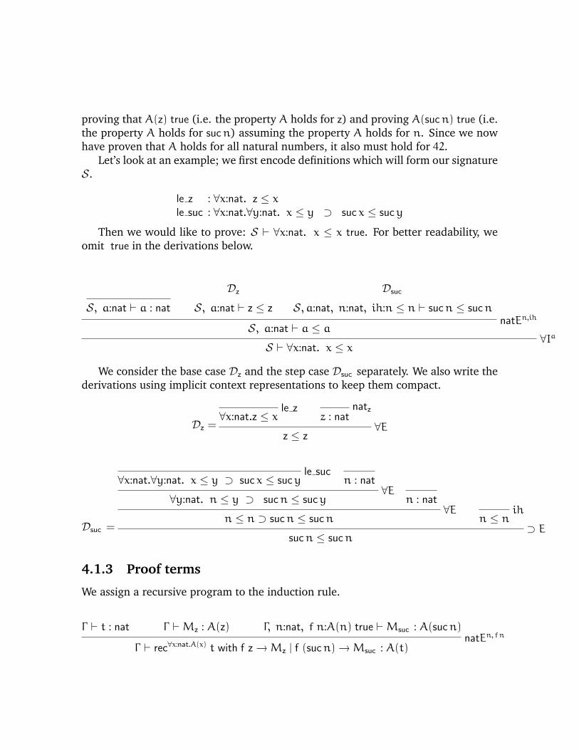
proving that A(z) true (i.e. the property A holds for z) and proving A(sucn) true (i.e.the property A holds for sucn) assuming the property A holds for n. Since we nowhave proven that A holds for all natural numbers, it also must hold for 42.

Let’s look at an example; we first encode definitions which will form our signatureS.

le z : ∀x:nat. z ≤ xle suc : ∀x:nat.∀y:nat. x ≤ y ⊃ suc x ≤ sucy

Then we would like to prove: S ` ∀x:nat. x ≤ x true. For better readability, weomit true in the derivations below.

S, a:nat ` a : nat

Dz

S, a:nat ` z ≤ z

Dsuc

S, a:nat, n:nat, ih:n ≤ n ` sucn ≤ sucnnatEn,ih

S, a:nat ` a ≤ a∀Ia

S ` ∀x:nat. x ≤ x

We consider the base case Dz and the step case Dsuc separately. We also write thederivations using implicit context representations to keep them compact.

Dz =

le z∀x:nat.z ≤ x

natzz : nat

∀Ez ≤ z

Dsuc =

le suc∀x:nat.∀y:nat. x ≤ y ⊃ suc x ≤ sucy n : nat

∀E∀y:nat. n ≤ y ⊃ sucn ≤ sucy n : nat

∀En ≤ n ⊃ sucn ≤ sucn

ihn ≤ n

⊃ Esucn ≤ sucn

4.1.3 Proof terms

We assign a recursive program to the induction rule.

Γ ` t : nat Γ `Mz : A(z) Γ, n:nat, f n:A(n) true `Msuc : A(sucn)natEn, f n

Γ ` rec∀x:nat.A(x) t with f z →Mz | f (sucn) →Msuc : A(t)

The proof term uses the variable f to denote the function we are defining; in somesense, this definition is similar to programs allowing defining functions by equationsusing simultaneous pattern as in Haskell.

From the proof above for S ` ∀x:nat. x ≤ x we can synthesize the followingprogram:

λa:nat. rec∀x:nat. x≤x a with| f z ⇒ le z z| f (sucn) ⇒ le suc nn (f n)

How to extend our notion of computation? We will have two reduction ruleswhich allow us to reduce a recursive program:

recA z with f z →Mz | f (sucn) →Msuc =⇒ Mz

recA (suc t) with f z →Mz | f (sucn) →Msuc =⇒ [t/n][r/f n]Msuc

where r = recA t with f z →Mz | f (sucn) →Msuc

Note that we unroll the recursion by replacing the reference to the recursive callf n with the actual recursive program recA t with f z →Mz | f (sucn) →Msuc .

We might ask, how to extend our congruence rules. In our setting, were reduc-tions can happen at any given sub-term, we will have two additional congruencerules. Note that we do not have a rule which evaluates t, the term we are recursingover; at the moment, the only possible terms we can have are those formed by z andsuc or variables. We have no computational power on for terms t of our domain.

Congruence rules

Nz =⇒ N ′z

recA t with f z → Nz | f (sucn) → Nsuc =⇒ recA t with f z → N ′z | f (sucn) → Nsuc

Nsuc =⇒ N ′suc

recA t with f z → Nz | f (sucn) → Nsuc =⇒ recA t with f z → Nz | f (sucn) → N ′suc

Proving subject reduction We also revisit subject reduction, showing that the ad-ditional rules for recursion preserve types. This is a good check that we didn’t screwup.

Theorem 4.1.1. If M =⇒M ′ and Γ `M : C then Γ `M ′ : C.

Proof. By structural induction on M =⇒M ′.

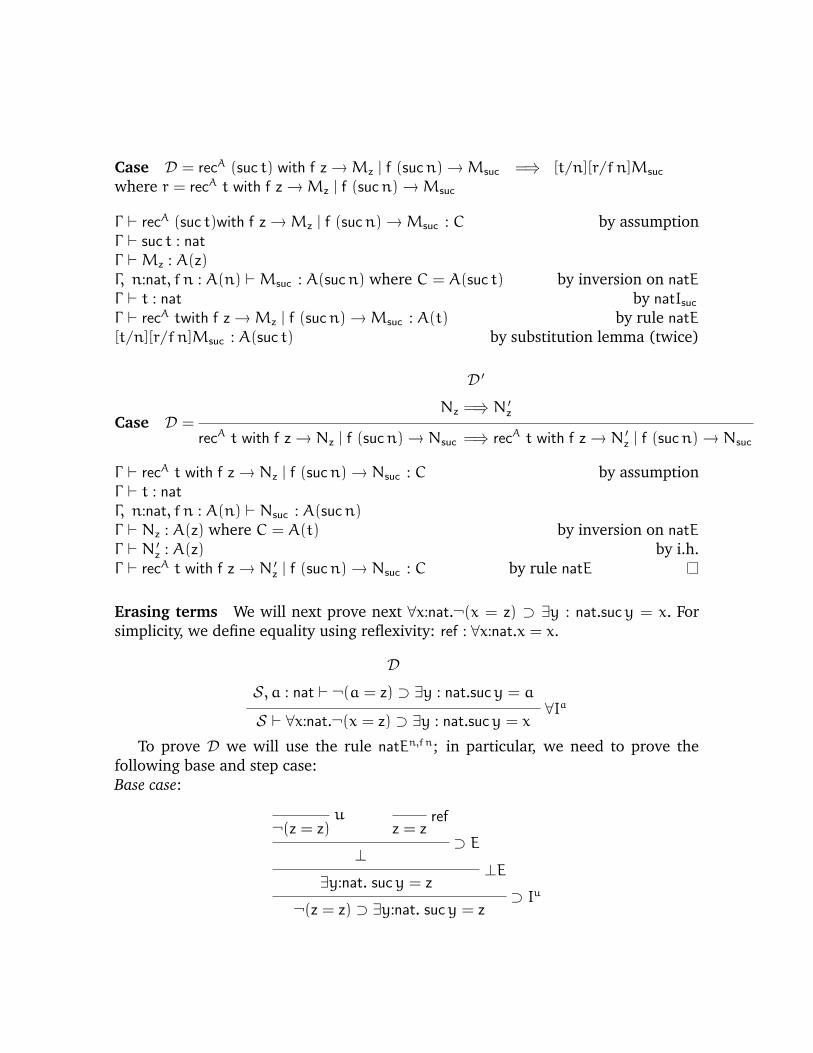
Case D = recA (suc t) with f z →Mz | f (sucn) →Msuc =⇒ [t/n][r/f n]Msuc

where r = recA t with f z →Mz | f (sucn) →Msuc

Γ ` recA (suc t)with f z →Mz | f (sucn) →Msuc : C by assumptionΓ ` suc t : natΓ `Mz : A(z)Γ, n:nat, f n : A(n) `Msuc : A(sucn) where C = A(suc t) by inversion on natEΓ ` t : nat by natIsucΓ ` recA twith f z →Mz | f (sucn) →Msuc : A(t) by rule natE[t/n][r/f n]Msuc : A(suc t) by substitution lemma (twice)

Case D =

D ′

Nz =⇒ N ′z

recA t with f z → Nz | f (sucn) → Nsuc =⇒ recA t with f z → N ′z | f (sucn) → Nsuc

Γ ` recA t with f z → Nz | f (sucn) → Nsuc : C by assumptionΓ ` t : natΓ, n:nat, f n : A(n) ` Nsuc : A(sucn)Γ ` Nz : A(z) where C = A(t) by inversion on natEΓ ` N ′z : A(z) by i.h.Γ ` recA t with f z → N ′z | f (sucn) → Nsuc : C by rule natE

Erasing terms We will next prove next ∀x:nat.¬(x = z) ⊃ ∃y : nat.sucy = x. Forsimplicity, we define equality using reflexivity: ref : ∀x:nat.x = x.

D

S, a : nat ` ¬(a = z) ⊃ ∃y : nat.sucy = a∀Ia

S ` ∀x:nat.¬(x = z) ⊃ ∃y : nat.sucy = x

To prove D we will use the rule natEn,f n; in particular, we need to prove thefollowing base and step case:Base case:

u¬(z = z)

refz = z

⊃ E⊥

⊥E∃y:nat. sucy = z

⊃ Iu¬(z = z) ⊃ ∃y:nat. sucy = z

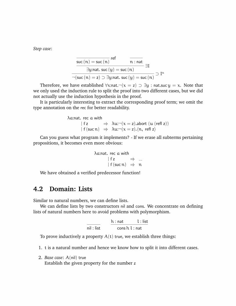
Step case:

refsuc (n) = suc (n) n : nat

∃I∃y:nat. suc (y) = suc (n)

⊃ Iu¬(suc (n) = z) ⊃ ∃y:nat. suc (y) = suc (n)

Therefore, we have established ∀x:nat.¬(x = z) ⊃ ∃y : nat.sucy = x. Note thatwe only used the induction rule to split the proof into two different cases, but we didnot actually use the induction hypothesis in the proof.

It is particularly interesting to extract the corresponding proof term; we omit thetype annotation on the rec for better readability.

λa:nat. rec a with| f z ⇒ λu:¬(x = z).abort (u (refl z))| f (sucn) ⇒ λu:¬(x = z).〈n, refl z〉

Can you guess what program it implements? - If we erase all subterms pertainingpropositions, it becomes even more obvious:

λa:nat. rec a with| f z ⇒| f (sucn) ⇒ n

We have obtained a verified predecessor function!

4.2 Domain: Lists

Similar to natural numbers, we can define lists.We can define lists by two constructors nil and cons. We concentrate on defining

lists of natural numbers here to avoid problems with polymorphism.

nil : list

h : nat l : list

consh l : nat

To prove inductively a property A(t) true, we establish three things:

1. t is a natural number and hence we know how to split it into different cases.

2. Base case: A(nil) trueEstablish the given property for the number z

3. Step case: For any h : nat, t : list, assumeA(t) true (I.H) and proveA(consh t) true.We assume the property holds for smaller lists, i.e. for t, and we establish theproperty for cons h t.

More formally the induction rule then takes on the following form:

Γ ` s : list Γ ` A(nil) Γ, n : nat, t : list, ih : A(t) ` A(cons n t)listEn,t,ih

Γ ` A(s)

The corresponding annotated rule takes on the form below giving us the abilityto write recursive functions about lists.

Γ ` s : list Γ `Mnil : A(nil) Γ, h:nat, t:list, f t:A(t) true `Mcons : A(cons h t)listEn, f n

Γ ` rec∀x:list.A(x) s with f nil →Mnil | f (cons h t) →Mcons : A(s)

recA nil with f nil →Mnil | f (cons h t) →Mcons =⇒ Mnil

recA (cons h ′ t ′) with f nil →Mnil | f (cons h t) →Mcons =⇒ [h ′/h][t ′/t][r/f t]Mcons

where r = recA t ′ with f nil →Mnil | f (cons h t) →Mcons

Let’s practice writing recursive functions. How would we write the function whichgiven a list reverses it. Its type is: T = list ⊃ list. We will write it in a tail-recursivemanner and write first a helper function of type S = list ⊃ list ⊃ list.

Λl : list.recS l with f nil → Λr : list.r | f (cons h t) → Λr : list.f t (cons h r)

4.3 Extending the induction principle to reasoning aboutindexed lists and other predicates

Often when we want to program with lists, we want more guarantees than simplythat given a list, we return a list. In the previous example, we might want to say thatgiven a list l1 of length n1 and an accumulator l2 of length n2, we return a list l3 ofn3 where n3 = n1 + n2.

First, how can we define lists which keep track of their length?

nil : list z

h : nat l : list n

cons {n} h l : list sucn

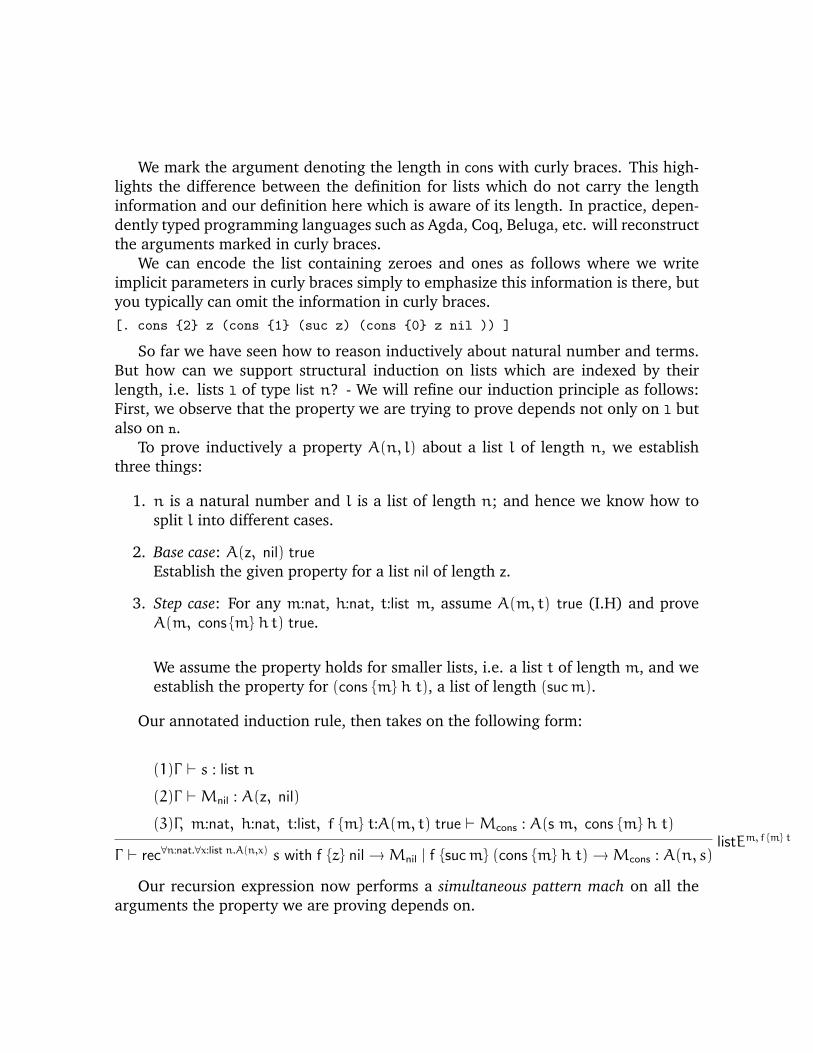
We mark the argument denoting the length in cons with curly braces. This high-lights the difference between the definition for lists which do not carry the lengthinformation and our definition here which is aware of its length. In practice, depen-dently typed programming languages such as Agda, Coq, Beluga, etc. will reconstructthe arguments marked in curly braces.

We can encode the list containing zeroes and ones as follows where we writeimplicit parameters in curly braces simply to emphasize this information is there, butyou typically can omit the information in curly braces.[. cons {2} z (cons {1} (suc z) (cons {0} z nil )) ]

So far we have seen how to reason inductively about natural number and terms.But how can we support structural induction on lists which are indexed by theirlength, i.e. lists l of type list n? - We will refine our induction principle as follows:First, we observe that the property we are trying to prove depends not only on l butalso on n.

To prove inductively a property A(n, l) about a list l of length n, we establishthree things:

1. n is a natural number and l is a list of length n; and hence we know how tosplit l into different cases.

2. Base case: A(z, nil) trueEstablish the given property for a list nil of length z.

3. Step case: For any m:nat, h:nat, t:list m, assume A(m, t) true (I.H) and proveA(m, cons {m} h t) true.

We assume the property holds for smaller lists, i.e. a list t of length m, and weestablish the property for (cons {m} h t), a list of length (sucm).

Our annotated induction rule, then takes on the following form:

(1)Γ ` s : list n

(2)Γ `Mnil : A(z, nil)

(3)Γ, m:nat, h:nat, t:list, f {m} t:A(m, t) true `Mcons : A(s m, cons {m} h t)listEm, f {m} t

Γ ` rec∀n:nat.∀x:list n.A(n,x) s with f {z} nil →Mnil | f {sucm} (cons {m} h t) →Mcons : A(n, s)

Our recursion expression now performs a simultaneous pattern mach on all thearguments the property we are proving depends on.

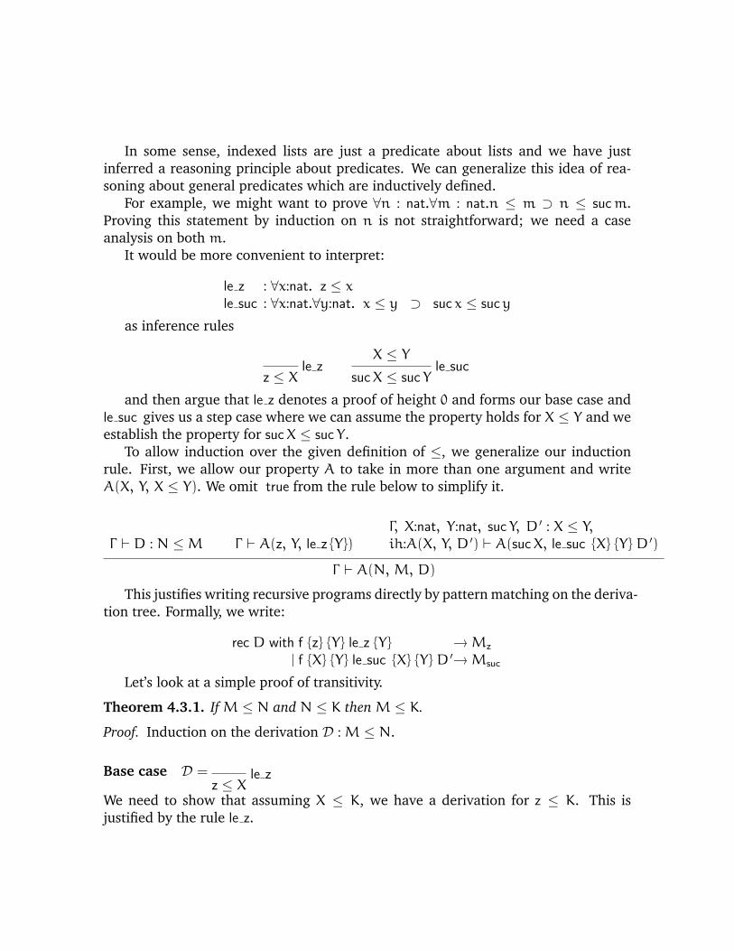
In some sense, indexed lists are just a predicate about lists and we have justinferred a reasoning principle about predicates. We can generalize this idea of rea-soning about general predicates which are inductively defined.

For example, we might want to prove ∀n : nat.∀m : nat.n ≤ m ⊃ n ≤ sucm.Proving this statement by induction on n is not straightforward; we need a caseanalysis on both m.

It would be more convenient to interpret:

le z : ∀x:nat. z ≤ xle suc : ∀x:nat.∀y:nat. x ≤ y ⊃ suc x ≤ sucy

as inference rules

le zz ≤ X

X ≤ Yle suc

sucX ≤ suc Y

and then argue that le z denotes a proof of height 0 and forms our base case andle suc gives us a step case where we can assume the property holds for X ≤ Y and weestablish the property for sucX ≤ suc Y.

To allow induction over the given definition of ≤, we generalize our inductionrule. First, we allow our property A to take in more than one argument and writeA(X, Y, X ≤ Y). We omit true from the rule below to simplify it.

Γ, X:nat, Y:nat, suc Y, D ′ : X ≤ Y,Γ ` D : N ≤M Γ ` A(z, Y, le z {Y}) ih:A(X, Y, D ′) ` A(sucX, le suc {X} {Y} D ′)

Γ ` A(N, M, D)

This justifies writing recursive programs directly by pattern matching on the deriva-tion tree. Formally, we write:

rec D with f {z} {Y} le z {Y} →Mz

| f {X} {Y} le suc {X} {Y} D ′→Msuc

Let’s look at a simple proof of transitivity.

Theorem 4.3.1. If M ≤ N and N ≤ K then M ≤ K.

Proof. Induction on the derivation D :M ≤ N.

Base case D = le zz ≤ X

We need to show that assuming X ≤ K, we have a derivation for z ≤ K. This isjustified by the rule le z.

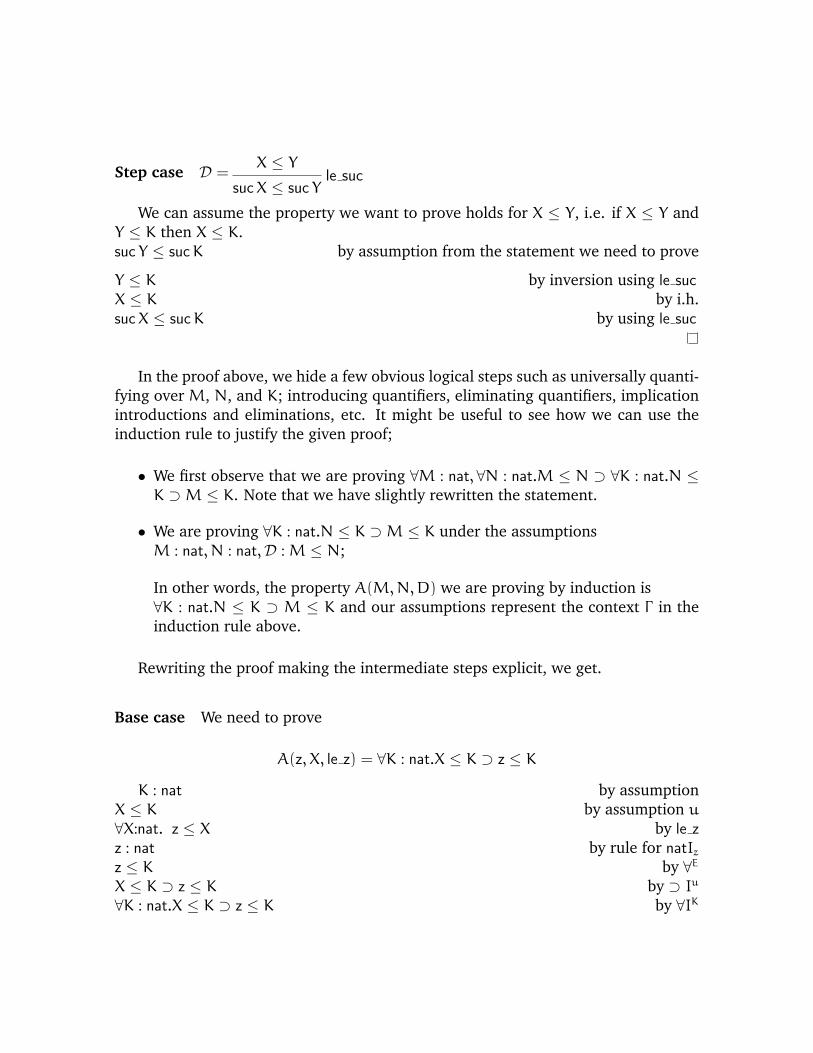
Step case D =X ≤ Y

le sucsucX ≤ suc Y

We can assume the property we want to prove holds for X ≤ Y, i.e. if X ≤ Y andY ≤ K then X ≤ K.suc Y ≤ sucK by assumption from the statement we need to prove

Y ≤ K by inversion using le sucX ≤ K by i.h.sucX ≤ sucK by using le suc

In the proof above, we hide a few obvious logical steps such as universally quanti-fying over M, N, and K; introducing quantifiers, eliminating quantifiers, implicationintroductions and eliminations, etc. It might be useful to see how we can use theinduction rule to justify the given proof;

• We first observe that we are proving ∀M : nat, ∀N : nat.M ≤ N ⊃ ∀K : nat.N ≤K ⊃M ≤ K. Note that we have slightly rewritten the statement.

• We are proving ∀K : nat.N ≤ K ⊃M ≤ K under the assumptionsM : nat, N : nat,D :M ≤ N;

In other words, the property A(M,N,D) we are proving by induction is∀K : nat.N ≤ K ⊃ M ≤ K and our assumptions represent the context Γ in theinduction rule above.

Rewriting the proof making the intermediate steps explicit, we get.

Base case We need to prove

A(z, X, le z) = ∀K : nat.X ≤ K ⊃ z ≤ K

K : nat by assumptionX ≤ K by assumption u∀X:nat. z ≤ X by le zz : nat by rule for natIzz ≤ K by ∀EX ≤ K ⊃ z ≤ K by ⊃ Iu∀K : nat.X ≤ K ⊃ z ≤ K by ∀IK

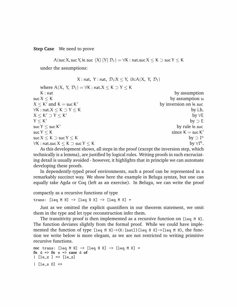
Step Case We need to prove

A(sucX, suc Y, le suc {X} {Y} D1) = ∀K : nat.sucX ≤ K ⊃ suc Y ≤ K

under the assumptions:

X : nat, Y : nat, D1:X ≤ Y, ih:A(X, Y, D1)

where A(X, Y, D1) = ∀K : nat.X ≤ K ⊃ Y ≤ KK : nat by assumption

sucX ≤ K by assumption uX ≤ K ′ and K = sucK ′ by inversion on le suc∀K : nat.X ≤ K ⊃ Y ≤ K by i.h.X ≤ K ′ ⊃ Y ≤ K ′ by ∀EY ≤ K ′ by ⊃ Esuc Y ≤ sucK ′ by rule le sucsuc Y ≤ K since K = sucK ′

sucX ≤ K ⊃ suc Y ≤ K by ⊃ Iu∀K : nat.sucX ≤ K ⊃ suc Y ≤ K by ∀IK.

As this development shows, all steps in the proof (except the inversion step, whichtechnically is a lemma), are justified by logical rules. Writing proofs in such excruciat-ing detail is usually avoided - however, it highlights that in principle we can automatedeveloping these proofs.

In dependently-typed proof environments, such a proof can be represented in aremarkably succinct way. We show here the example in Beluga syntax, but one canequally take Agda or Coq (left as an exercise). In Beluga, we can write the proof

compactly as a recursive functions of typetrans: [leq M N] -> [leq N K] -> [leq M K] =

Just as we omitted the explicit quantifiers in our theorem statement, we omitthem in the type and let type reconstruction infer them.

The transitivity proof is then implemented as a recursive function on [leq M N].The function deviates slightly from the formal proof. While we could have imple-mented the function of type [leq M N]->{K:[nat]}[leq N K]->[leq M N}, the func-tion we write below is more elegant, as we are not restricted to writing primitiverecursive functions.rec trans: [leq M N] -> [leq N K] -> [leq M K] =fn d => fn e => case d of| [le_z ] => [le_z]

| [le_s D] =>

let [le_s E] = e inlet [F] = trans [D] [E] in[le_s F]

;

We observe that every step in the proof corresponds exactly to one step in ourinformal proof; Beluga let’s you hide “logical” details (i.e. universal introduction andeliminations) which polluted our detailed formal proof above, but we concentrate onthe essential steps in the proof. Avoiding such clutter is essential in making writingrealistic proofs feasible!

To summarize:

On paper In BelugaCase analysis Case analysis

Appeal to induction hypothesis Recursive call

Inversion Case analysis with one caseusually using a let-expression

4.4 First-order Logic with Domain-specific Induction

More generally, we can extend our first-order logic with specific domains which wecall U. We embed predicates belonging to the domain U into first-order formulasusing the necessity modality, written as [U]. This is related to Moggi’s monadic lan-guage. Here we separate domain-specific definitions/knowledge from our genericfirst-order logic.

To support inductive reasoning about a domain U we need the domain to havecertain properties: for example it must be decidable when two objects of the domainU are equal. We also must have a way of splitting an object into different cases andhave a measure according to which an object of the domain is considered smallerthan another object. These ingredients are essential to generate induction principlesfor the given domain.

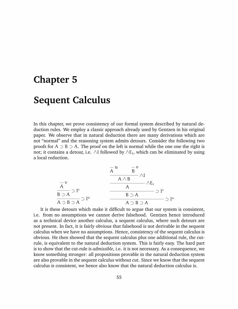
Chapter 5

Sequent Calculus

In this chapter, we prove consistency of our formal system described by natural de-duction rules. We employ a classic approach already used by Gentzen in his originalpaper. We observe that in natural deduction there are many derivations which arenot “normal” and the reasoning system admits detours. Consider the following twoproofs for A ⊃ B ⊃ A. The proof on the left is normal while the one one the right isnot; it contains a detour, i.e. ∧I followed by ∧El, which can be eliminated by usinga local reduction.

vA

⊃ IvB ⊃ A

⊃ IuA ⊃ B ⊃ A

uA

vB

∧IA∧ B

∧ElA

⊃ IvB ⊃ A

⊃ IuA ⊃ B ⊃ A

It is these detours which make it difficult to argue that our system is consistent,i.e. from no assumptions we cannot derive falsehood. Gentzen hence introducedas a technical device another calculus, a sequent calculus, where such detours arenot present. In fact, it is fairly obvious that falsehood is not derivable in the sequentcalculus when we have no assumptions. Hence, consistency of the sequent calculus isobvious. He then showed that the sequent calculus plus one additional rule, the cut-rule, is equivalent to the natural deduction system. This is fairly easy. The hard partis to show that the cut-rule is admissible, i.e. it is not necessary. As a consequence, weknow something stronger: all propositions provable in the natural deduction systemare also provable in the sequent calculus without cut. Since we know that the sequentcalculus is consistent, we hence also know that the natural deduction calculus is.

55

The sequent calculus is not only of interest because it is a convenient technicaldevice for establishing consistency of natural deduction. It also gives rise to proofsearch procedures. In fact, we can study its proof-theoretic properties further andarrive at proof systems where proof search is feasible and amendable to efficientimplementations.

5.1 Normal Natural Deductions

As a technical device, we introduce a natural deduction calculus where we restrictderivations to normal derivations, i.e. derivations which do not admit detours. Aswe have seen when we considered proof terms for the natural deduction system, adetour meant we had a redex in our proof term, i.e. a subterm which can be reduced;our proof term is in normal form. In fact, it might be helpful to consider the subset ofterms consisting of lambda-terms, applications, pairs and projections to characterizenormal forms more precisely. We will subsequently add the other proof terms as well.

Normal Terms M,N ::= λx:A.M | 〈M, N〉 | () | RNeutral Terms R ::= x | fst R | snd R | R N

As we can see, a term λx:A.(λy:A.y) x is not valid normal term, because we havea redex (λy:A.y) x which reduces to x. According to our grammar of normal andneutral terms (λy:A.y) x is ill-formed.

The normal natural deduction calculus, the proof calculus which only admits nor-mal terms, captures also a very intuitive simple strategy which we already used in-formally when constructing proofs. When proving a proposition, we use introductionrules reasoning bottom-up (from the proposed theorem towards the hypothesis) andelimination rules top-down (from the assumptions towards the proposed theorem)meeting the result of the intro-rules.

We will introduce two new judgements to describe this proof strategy:

M : A ↑ Proposition A has a normal deduction described by the normal term M

R : A ↓ Proposition A is extracted from a hypothesis described the the neutral term R

We immediately give the judgements annotated with proof terms; this highlightsthat we are only constructing normal terms. However, we will often simply writeA ↑ and A ↓ , if the proof term itself is not of interest to us.

All assumptions will be written as x : A ↓ , and hence the localized form, i.e. theform where explicitly list our assumptions, can be described as

u1:A1 ↓ , . . . , un:An ↓ ` M : A ↑u1:A1 ↓ , . . . , un:An ↓ ` R : A ↓

We write Γ ↓ for a context u1:A1 ↓ , . . . , un:An ↓ .Let us know revisit the natural deduction rules.

Hypothesis The general hypothesis rule simply reflects the fact that from a list ofassumptions, we can extract one.

uΓ ↓1 , u:A ↓ , Γ ↓2 ` u : A ↓

Coercion The introduction and elimination rules must be able to meet and we needto be able to switch to extracting information from the assumptions. From the proofterm point of view, every neutral term is also a normal term. This is achieved by acoercion.

Γ ↓ ` R : A ↓ ↓ ↑Γ ↓ ` R : A ↑

Note that the opposite direction is not allowed; not all normal terms are neutralterms. It would also contradict our intended strategy.

Conjunction The rules for conjunction are straightforward.

Γ ↓ `M : A ↑ Γ ↓ ` N : B ↑∧I

Γ ↓ ` 〈M, N〉 : A∧ B ↑Γ ↓ ` R : A∧ B ↓

∧ElΓ ↓ ` fst R : A ↓ Γ ↓ ` R : A∧ B ↓

∧ErΓ ↓ ` snd M : B ↓

Truth The rule for truth, is also straightforward. As it is an introduction rule, itconstructs a normal derivation.

>IΓ ↓ ` () : > ↑

Implication The rule for implication follows a similar recipe as before. In the in-troduction rule, we add a new assumption labelled as neutral. In the eliminationrule, we extract from the assumptions in Γ ↓ a proof R for A ⊃ B; we now can verifythat A has a normal derivation described by M and are able to extract a proof for Bdescribed by the neutral term R M.

Γ ↓, u:A ↓`M : B ↑⊃ Iu

Γ ↓ ` λx:A.M : A ⊃ B ↑ Γ ↓ ` R : A ⊃ B ↓ Γ ↓ `M : A ↑⊃ E

Γ ↓ ` R M : B ↓Disjunction The introduction rules can easily be annotated with norm. For theelimination rule we again extract the premise A∨B, hence annotating it with ↓ . Wechoose to identify the main conclusion C with a normal term annotating it with ↑ .

Γ ↓ `M : A ↑∨Il

Γ ↓ ` inlA M : A∨ B ↑ Γ ↓ ` N : B ↑∨Ir

Γ ↓ ` inrB N : A∨ B ↑Γ ↓ ` R : A∨ B ↓ Γ ↓, x:A ↓`Ml : C ↑ Γ ↓, y:B ↓`Mr : C ↑

∨Ex,y

Γ ↓ ` case R of inlA x→Ml | inrB y→Mr : C ↑It would also be consistent to allow the derivations of C to be extractions, but it is

not necessary to obtain a complete search procedure and complicates the relation tothe sequent calculus. It also complicates our computational reading of the disjunc-tion rule, since it would mean we extract a proposition Cl in the first branch and a(possibly another) proposition Cr in the second branch, and we then need to checkthat they are the same.

Falsehood If we can synthesize a contradiction, then we have constructed a prooffor C. It would not make sense to have C being synthesized, i.e. being annotatedwith ↓ , since it would be completely unrestricted.

Γ ↓ ` R : ⊥ ↓⊥E

abortC M : C ↑Exercise 5.1.1.

Annotate the rules for universal and existential quantifiers

Exercise 5.1.2.

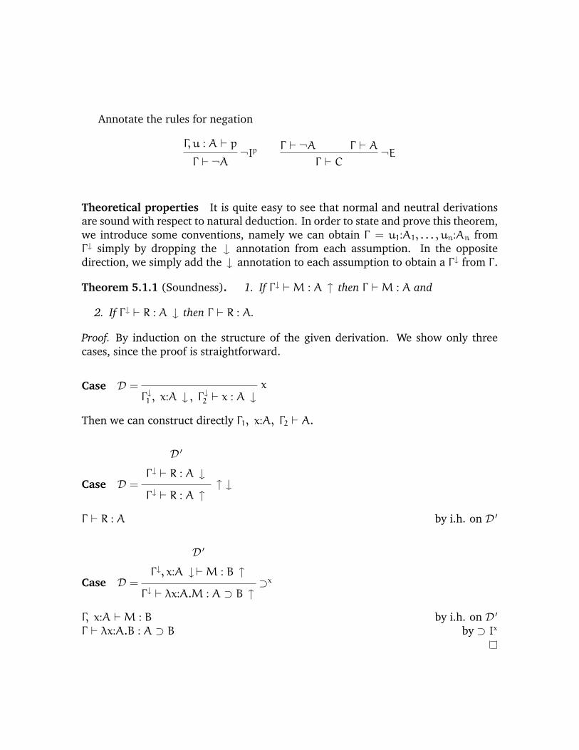
Annotate the rules for negation

Γ, u : A ` p¬Ip

Γ ` ¬A

Γ ` ¬A Γ ` A¬E

Γ ` C

Theoretical properties It is quite easy to see that normal and neutral derivationsare sound with respect to natural deduction. In order to state and prove this theorem,we introduce some conventions, namely we can obtain Γ = u1:A1, . . . , un:An fromΓ ↓ simply by dropping the ↓ annotation from each assumption. In the oppositedirection, we simply add the ↓ annotation to each assumption to obtain a Γ ↓ from Γ .

Theorem 5.1.1 (Soundness). 1. If Γ ↓ `M : A ↑ then Γ `M : A and

2. If Γ ↓ ` R : A ↓ then Γ ` R : A.

Proof. By induction on the structure of the given derivation. We show only threecases, since the proof is straightforward.

Case D = xΓ ↓1 , x:A ↓ , Γ ↓2 ` x : A ↓

Then we can construct directly Γ1, x:A, Γ2 ` A.

Case D =

D ′

Γ ↓ ` R : A ↓ ↑ ↓Γ ↓ ` R : A ↑

Γ ` R : A by i.h. on D ′

Case D =

D ′

Γ ↓, x:A ↓`M : B ↑⊃x

Γ ↓ ` λx:A.M : A ⊃ B ↑Γ, x:A `M : B by i.h. on D ′Γ ` λx:A.B : A ⊃ B by ⊃ Ix

However, we note that we restricted what derivations we allow; so clearly, it isnot obvious that we can translate every natural deduction derivation into a normalnatural deduction proof. For example, the derivation we have given at the beginningof the chapter cannot be annotated with our rules.

uA ↓ v

B ↓??

A∧ B ↑ ↓A ↓

∧ElA ↑

⊃ IvB ⊃ A ↑

⊃ IuA ⊃ B ⊃ A ↑

The problem is that while from A∧B ↓ we can extract A ↓ , we cannot constructA∧B ↓ . Given our assumptions A ↓ we can turn it into A ↑ ; similarly, we can turnB ↓ into B ↑ , and conclude A ∧ B ↑ . But there is not way to go from A ∧ B ↑ toA∧ B ↓ - only the opposite direction is allowed!

To resurrect completeness, we temporarily allow the conversion

Γ ↓ `M : A ↑ ↓ ↑Γ ↓ ` (M:A) : A ↓

Computationally, we can read this rule as follows: we can synthesize a type A forthe expression M : A, if M checks against A. We keep the proposition we check Magainst as part of the proof term we construct as evidence in the conclusion. Hence,this rule allows explicit type annotations where we transition.

With this rule ↓ ↑ we can now of course translate also the non-normal derivationabove. We will distinguish between the bi-directional natural deduction system with↓ ↑ rule, written as Γ ↓ `+ J, and the bi-direction natural deduction system without↓ ↑ , written as Γ ↓ ` J. In other words Γ ↓ `+ J contains all the bi-directional rulesfrom Γ ↓ ` J, but in addition we can mark and identify the transitions where ourderivation is not normal. These places are justified by the ↓ ↑ rule.

Γ ↓ ` M : A ↑Γ ↓ ` R : A ↓ Characterize only normal derivations

Γ ↓ `+ M : A ↑Γ ↓ `+ R : A ↓ Characterize all normal derivations and identify non-

normal derivations via the rule ↓ ↑ .

It is easy to show that the extended bi-directional natural deduction system issound and complete with respect to the original natural natural deduction system.

Theorem 5.1.2 (Soundness).

1. If Γ ↓ `+ M : A ↑ then Γ `M : A.

2. If Γ ↓ `+ R : A ↓ then Γ ` R : A.

Proof. By simultaneous structural induction over the structure of the given deriva-tions.

Since adding proof terms complicates the completeness theorem and the proofslightly, we omit the proof terms in the statement and proof below. In essence, theproof terms we have in the original system are not exactly the same as the ones inthe bi-directional system, because we have type annotations at normal terms whichare embedded within neutral terms.

Theorem 5.1.3 (Completeness of annotated natural deduction).

1. If Γ ` A then Γ ↓ `+ A ↑ and Γ ↓ `+ A ↓ .

Proof. By induction over the structure of the given derivation. We show only twocases. We often refer to Γ ↓ `+ A ↑ as (1) and Γ ↓ `+ A ↓ as (2).

Case D =

D1Γ ` A ⊃ B

D2Γ ` A

⊃ EΓ ` B

Γ ↓ ` A ⊃ B ↓ by i.h. (2)Γ ↓ ` A ↑ by i.h. (1)Γ ↓ ` B ↓ by ⊃ E proving (2)Γ ↓ ` B ↑ by ↑ ↓ , proving (1)

Case D =

D1Γ, x:A ` B

⊃ IxΓ ` A ⊃ B

Γ ↓, x:A ↓` B ↑ by i.h. (1)Γ ↓ ` A ⊃ B ↑ by ⊃ Ix proving (1)Γ ↓ ` A ⊃ B ↓ by ↓ ↑ proving (2)

Note that although natural deduction and bi-directional natural deduction ex-tended with ↓ ↑ rule are very similar, they are not in a bijective correspondence.In the bi-directional natural deduction system we can simply alternate the two co-ercions an arbitrary number of times and they are identified explicitly, while in thenatural deduction system they are invisible.

Finally, we state some substitution properties for normal natural deductions. Theytake the following form.

Lemma 5.1.4 (Substitution property for normal natural deductions).

1. If Γ ↓1 , u:A ↓ , Γ ↓2 ` C ↑ and Γ ↓1 ` A ↓ then Γ ↓1 , Γ ↓2 ` C ↑ .

2. IF Γ ↓1 , u:A ↓ , Γ ↓2 ` C ↓ and Γ ↓1 ` A ↓ then Γ ↓1 , Γ ↓2 ` C ↓ .

Proof. By induction on the structure of the given derivation of C ↑ and C ↓ usingweakening.

5.1.1 Sequent calculus

In this section, we develop a closely related calculus to the bi-directional naturaldeduction system, called the sequent calculus. Studying meta-theoretical propertiessuch as consistency is easier in this system; moreover, it provides a good calculus forproof search.

In the bi-directional natural deduction calculus, we keep the context Γ ↓ for book-keeping, but all the action happens on the right hand side of `+ (or `). In particular,we switch from reasoning bottom-up via introduction rules to reasoning top-downvia elimination rules; this switch is identified by the ↑ ↓ rule.

In the sequent calculus, we only reason from the bottom-up by turning elimina-tion rules into left rules that directly manipulate our assumptions in the context Γ .The judgement for a sequent is written as:

u1:A1, . . . , un:An =⇒ C

Note that the proposition C on the right directly corresponds to the propositionwhose truth is established by a natural deduction. The propositions on the left how-ever do not directly correspond to hypothesis in natural deduction, since in generalthey include hypothesis and propositions derived from assumptions by eliminationrules. It is important to keep this difference in mind when we relate sequent proofsto natural deduction derivations.

Since the order of the propositions on the left is irrelevant, we write Γ, u:A insteadof the more pedantic Γ, u:A, Γ ′.

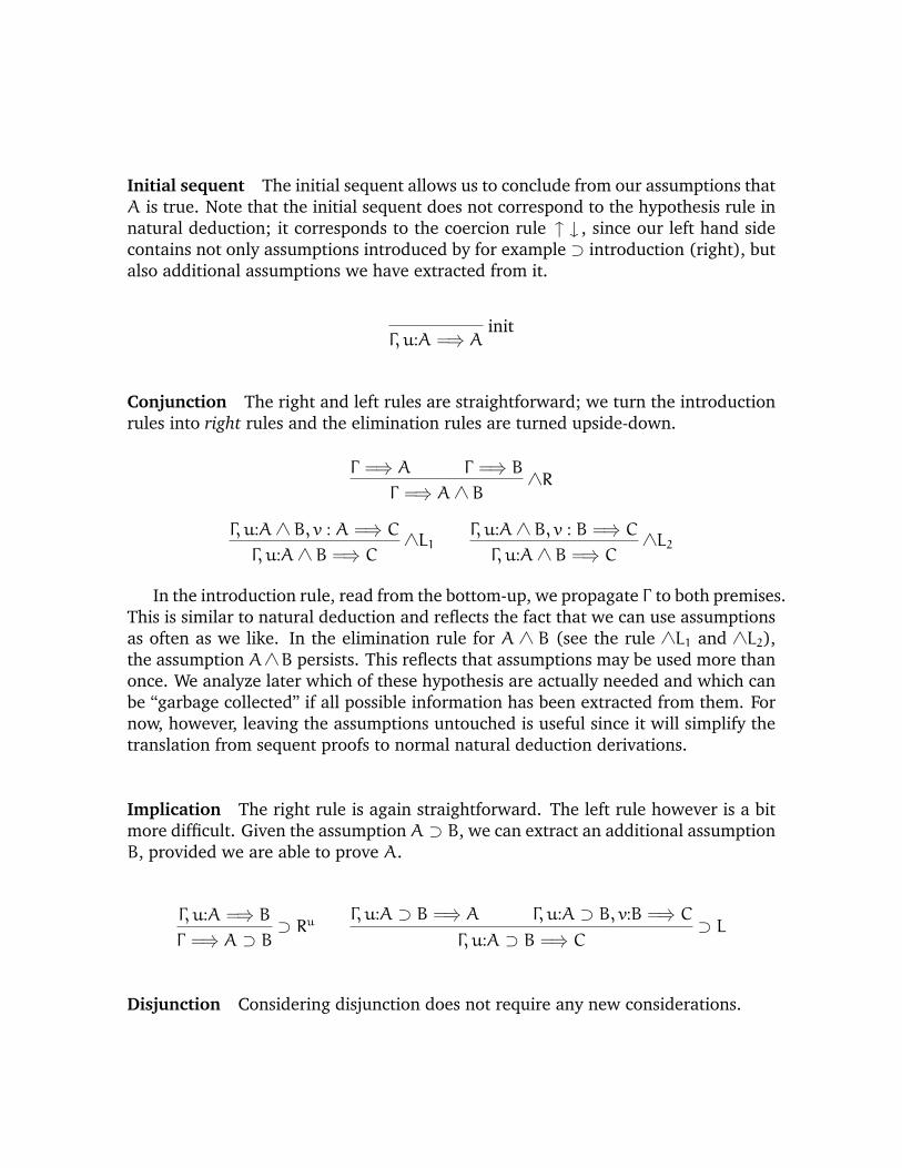
Initial sequent The initial sequent allows us to conclude from our assumptions thatA is true. Note that the initial sequent does not correspond to the hypothesis rule innatural deduction; it corresponds to the coercion rule ↑ ↓ , since our left hand sidecontains not only assumptions introduced by for example ⊃ introduction (right), butalso additional assumptions we have extracted from it.

initΓ, u:A =⇒ A

Conjunction The right and left rules are straightforward; we turn the introductionrules into right rules and the elimination rules are turned upside-down.

Γ =⇒ A Γ =⇒ B∧R

Γ =⇒ A∧ B

Γ, u:A∧ B, v : A =⇒ C∧L1

Γ, u:A∧ B =⇒ C

Γ, u:A∧ B, v : B =⇒ C∧L2

Γ, u:A∧ B =⇒ C

In the introduction rule, read from the bottom-up, we propagate Γ to both premises.This is similar to natural deduction and reflects the fact that we can use assumptionsas often as we like. In the elimination rule for A ∧ B (see the rule ∧L1 and ∧L2),the assumption A∧B persists. This reflects that assumptions may be used more thanonce. We analyze later which of these hypothesis are actually needed and which canbe “garbage collected” if all possible information has been extracted from them. Fornow, however, leaving the assumptions untouched is useful since it will simplify thetranslation from sequent proofs to normal natural deduction derivations.

Implication The right rule is again straightforward. The left rule however is a bitmore difficult. Given the assumptionA ⊃ B, we can extract an additional assumptionB, provided we are able to prove A.

Γ, u:A =⇒ B ⊃ RuΓ =⇒ A ⊃ B

Γ, u:A ⊃ B =⇒ A Γ, u:A ⊃ B, v:B =⇒ C⊃ L

Γ, u:A ⊃ B =⇒ C

Disjunction Considering disjunction does not require any new considerations.

Γ =⇒ A∨R1

Γ =⇒ A∨ B

Γ =⇒ B∨R2

Γ =⇒ A∨ B

Γ, u:A∨ B, v:A =⇒ C Γ, u:A∨ B,w:B =⇒ C∨Lv,w

Γ, u:A∨ B =⇒ C

Truth Since there is no elimination rule for >, we only have to consider the intro-duction rule which directly translates to a right rule in the sequent calculus.

>RΓ =⇒ >

Falsehood Since there is no introduction rule for ⊥, we only consider the elimina-tion rule which turns into a left rule.

⊥LΓ, u:⊥ =⇒ C

Note that the left rule has no premise.

Exercise 5.1.3.

Derive the rules for universal and existential quantifiers in the sequent calculus.

Exercise 5.1.4.

Derive the rules for negation in the sequent calculus form.

5.1.2 Theoretical properties of sequent calculus

We first begin by stating and revisiting some of the structural properties.

Lemma 5.1.5 (Structural properties of sequents).

1. (Weakening) If Γ =⇒ C then Γ, u:A =⇒ C.

2. (Contraction) If Γ, u:A, v:A =⇒ C then Γ, u:A =⇒ C.

Proof. By structural induction on the first derivation.

Next, we prove that our sequent calculus indeed characterizes normal naturaldeductions.

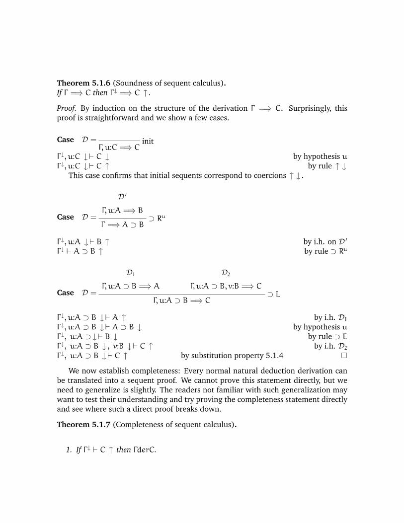
Theorem 5.1.6 (Soundness of sequent calculus).If Γ =⇒ C then Γ ↓ =⇒ C ↑ .

Proof. By induction on the structure of the derivation Γ =⇒ C. Surprisingly, thisproof is straightforward and we show a few cases.

Case D = initΓ, u:C =⇒ C

Γ ↓, u:C ↓` C ↓ by hypothesis uΓ ↓, u:C ↓` C ↑ by rule ↑ ↓

This case confirms that initial sequents correspond to coercions ↑ ↓ .

Case D =

D ′

Γ, u:A =⇒ B⊃ Ru

Γ =⇒ A ⊃ B

Γ ↓, u:A ↓` B ↑ by i.h. on D ′Γ ↓ ` A ⊃ B ↑ by rule ⊃ Ru

Case D =

D1Γ, u:A ⊃ B =⇒ A

D2Γ, u:A ⊃ B, v:B =⇒ C

⊃ LΓ, u:A ⊃ B =⇒ C

Γ ↓, u:A ⊃ B ↓` A ↑ by i.h. D1Γ ↓, u:A ⊃ B ↓` A ⊃ B ↓ by hypothesis uΓ ↓, u:A ⊃ ↓` B ↓ by rule ⊃ EΓ ↓, u:A ⊃ B ↓ , v:B ↓` C ↑ by i.h. D2Γ ↓, u:A ⊃ B ↓` C ↑ by substitution property 5.1.4

We now establish completeness: Every normal natural deduction derivation canbe translated into a sequent proof. We cannot prove this statement directly, but weneed to generalize is slightly. The readers not familiar with such generalization maywant to test their understanding and try proving the completeness statement directlyand see where such a direct proof breaks down.

Theorem 5.1.7 (Completeness of sequent calculus).

1. If Γ ↓ ` C ↑ then ΓderC.

2. If Γ ↓ ` A ↓ and Γ, u:A =⇒ C then Γ =⇒ C.

Proof. By structural induction on the structure of the given derivation Γ ↓ ` C ↑ andΓ ↓ ` A ↓ respectively.

Case D = uΓ ↓1 , u:A ↓ , Γ ↓2 ` A ↓

Γ1, u:A, Γ2, v:A =⇒ C by assumptionΓ1, u:A, Γ2 =⇒ C by contraction (Lemma 5.1.5)

Case D =

D ′

Γ ↓ ` C ↓ ↑ ↓Γ ↓ ` C ↑

Γ, u:C =⇒ C by initΓ =⇒ C by i.h. D ′

Case D =

D ′

Γ ↓, u:A ↓` B ↑⊃ Iu

Γ ↓ ` A ⊃ B ↑Γ, u:A =⇒ B by i.h. D ′Γ =⇒ A ⊃ B by ⊃ Ru

Case D =

D1Γ ↓ ` A ⊃ B ↓ D2

Γ ↓ ` A ↑⊃ E

Γ ↓ ` B ↓Γ, u:B =⇒ C by assumptionΓ,w:A ⊃ B, u:B =⇒ C by weakening (Lemma 5.1.5)Γ =⇒ A by i.h. D2Γ,w:A ⊃ B =⇒ C by ⊃ LΓ =⇒ C by i.h. D1

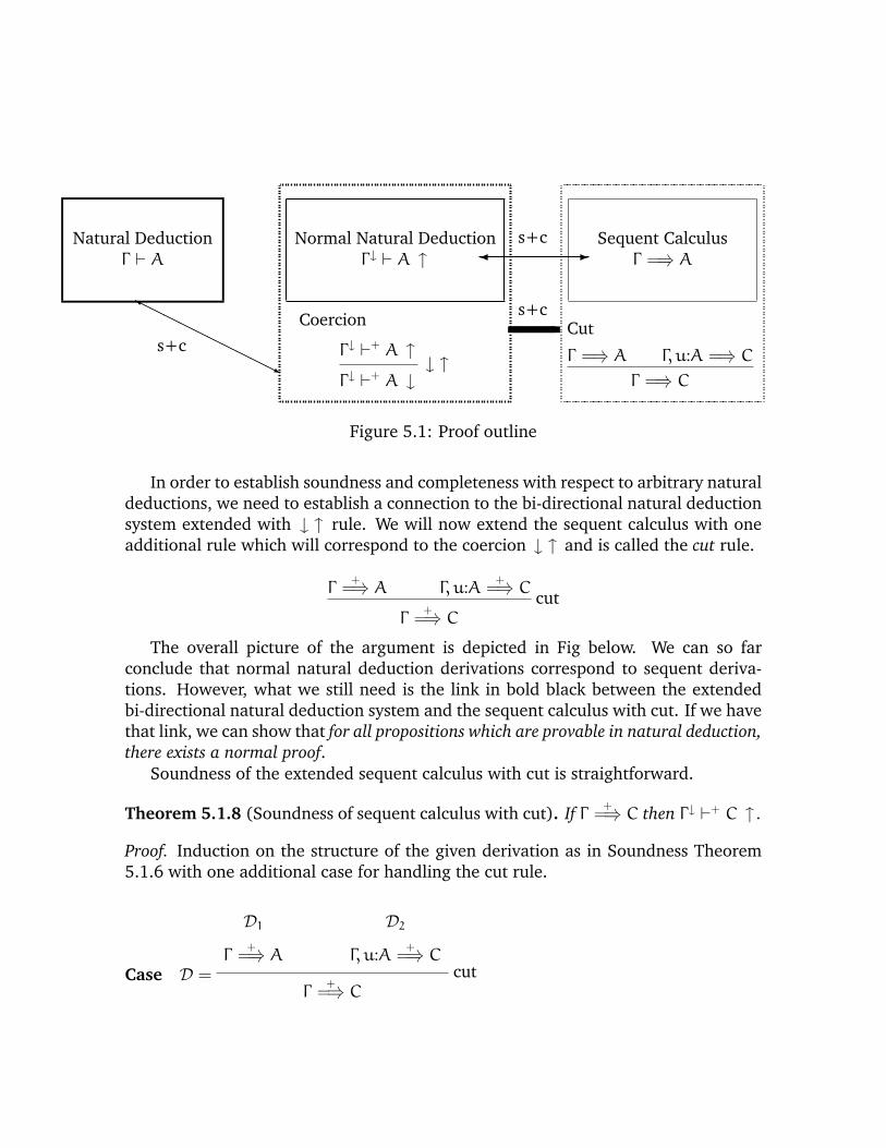
Natural DeductionΓ ` A

HHHHH

HHHHHYHHHHH

HHHHHj

s+cCoercion

Γ ↓ `+ A ↑ ↓ ↑Γ ↓ `+ A ↓

-�s+cNormal Natural Deduction

Γ ↓ ` A ↑Cut

Γ =⇒ A Γ, u:A =⇒ C

Γ =⇒ C

-�s+c

Sequent CalculusΓ =⇒ A

Figure 5.1: Proof outline

In order to establish soundness and completeness with respect to arbitrary naturaldeductions, we need to establish a connection to the bi-directional natural deductionsystem extended with ↓ ↑ rule. We will now extend the sequent calculus with oneadditional rule which will correspond to the coercion ↓ ↑ and is called the cut rule.

Γ+

=⇒ A Γ, u:A+

=⇒ Ccut

Γ+

=⇒ C

The overall picture of the argument is depicted in Fig below. We can so farconclude that normal natural deduction derivations correspond to sequent deriva-tions. However, what we still need is the link in bold black between the extendedbi-directional natural deduction system and the sequent calculus with cut. If we havethat link, we can show that for all propositions which are provable in natural deduction,there exists a normal proof.

Soundness of the extended sequent calculus with cut is straightforward.

Theorem 5.1.8 (Soundness of sequent calculus with cut). If Γ +=⇒ C then Γ ↓ `+ C ↑ .

Proof. Induction on the structure of the given derivation as in Soundness Theorem5.1.6 with one additional case for handling the cut rule.

Case D =

D1

Γ+

=⇒ A

D2

Γ, u:A+

=⇒ Ccut

Γ+

=⇒ C

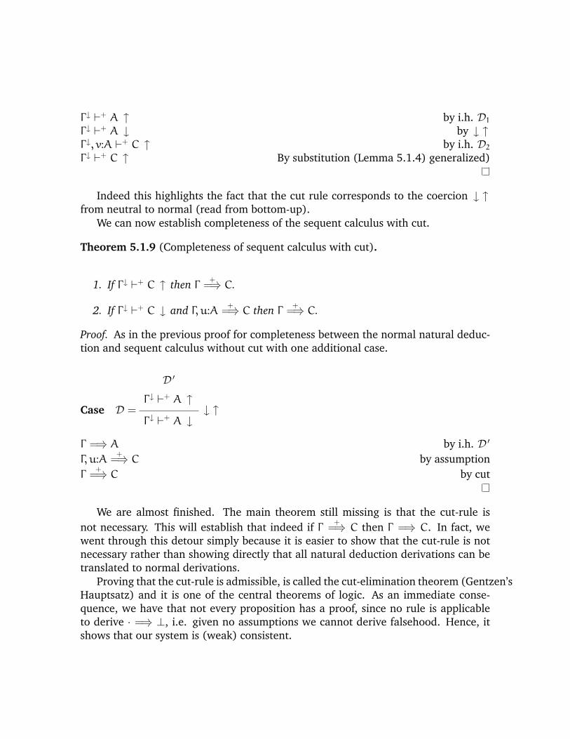
Γ ↓ `+ A ↑ by i.h. D1Γ ↓ `+ A ↓ by ↓ ↑Γ ↓, v:A `+ C ↑ by i.h. D2Γ ↓ `+ C ↑ By substitution (Lemma 5.1.4) generalized)

Indeed this highlights the fact that the cut rule corresponds to the coercion ↓ ↑from neutral to normal (read from bottom-up).

We can now establish completeness of the sequent calculus with cut.

Theorem 5.1.9 (Completeness of sequent calculus with cut).

1. If Γ ↓ `+ C ↑ then Γ +=⇒ C.

2. If Γ ↓ `+ C ↓ and Γ, u:A +=⇒ C then Γ +

=⇒ C.

Proof. As in the previous proof for completeness between the normal natural deduc-tion and sequent calculus without cut with one additional case.

Case D =

D ′

Γ ↓ `+ A ↑ ↓ ↑Γ ↓ `+ A ↓

Γ =⇒ A by i.h. D ′

Γ, u:A+

=⇒ C by assumptionΓ

+=⇒ C by cut

We are almost finished. The main theorem still missing is that the cut-rule isnot necessary. This will establish that indeed if Γ +

=⇒ C then Γ =⇒ C. In fact, wewent through this detour simply because it is easier to show that the cut-rule is notnecessary rather than showing directly that all natural deduction derivations can betranslated to normal derivations.

Proving that the cut-rule is admissible, is called the cut-elimination theorem (Gentzen’sHauptsatz) and it is one of the central theorems of logic. As an immediate conse-quence, we have that not every proposition has a proof, since no rule is applicableto derive · =⇒ ⊥, i.e. given no assumptions we cannot derive falsehood. Hence, itshows that our system is (weak) consistent.

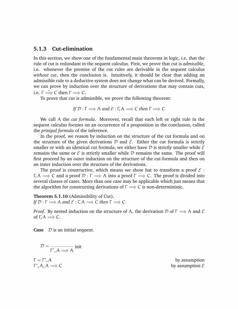
5.1.3 Cut-elimination

In this section, we show one of the fundamental main theorems in logic, i.e. that therule of cut is redundant in the sequent calculus. First, we prove that cut is admissible,i.e. whenever the premise of the cut rules are derivable in the sequent calculuswithout cut, then the conclusion is. Intuitively, it should be clear that adding anadmissible rule to a deductive system does not change what can be derived. Formally,we can prove by induction over the structure of derivations that may contain cuts,i.e. Γ +

=⇒ C then Γ =⇒ C.To prove that cut is admissible, we prove the following theorem:

If D : Γ =⇒ A and E : Γ,A =⇒ C then Γ =⇒ C

We call A the cut formula. Moreover, recall that each left or right rule in thesequent calculus focuses on an occurrence of a proposition in the conclusion, calledthe prinipal formula of the inference.

In the proof, we reason by induction on the structure of the cut formula and onthe structure of the given derivations D and E . Either the cut formula is strictlysmaller or with an identical cut formula, we either have D is strictly smaller while Eremains the same or E is strictly smaller while D remains the same. The proof willfirst proceed by an outer induction on the structure of the cut-formula and then onan inner induction over the structure of the derivations.

The proof is constructive, which means we show hat to transform a proof E :Γ,A =⇒ C and a proof D : Γ =⇒ A into a proof Γ =⇒ C. The proof is divided intoseveral classes of cases. More than one case may be applicable which just means thatthe algorithm for constructing derivations of Γ =⇒ C is non-deterministic.

Theorem 5.1.10 (Admissibility of Cut).If D : Γ =⇒ A and E : Γ,A =⇒ C then Γ =⇒ C.

Proof. By nested induction on the structure of A, the derivation D of Γ =⇒ A and Eof Γ,A =⇒ C.

Case D is an initial sequent.

D = initΓ ′, A =⇒ A

Γ = Γ ′, A by assumptionΓ ′, A,A =⇒ C by assumption E

Γ ′, A =⇒ C by contractionΓ =⇒ C

Case E is an initial sequent and uses the cut formula

E = initΓ,A =⇒ A

C = A by assumptionΓ =⇒ A by derivation D

Case E is an initial sequent and does not use the cut formula

E = initΓ ′, C,A =⇒ C

Γ = Γ ′, C by assumptionΓ ′, C =⇒ C by rule initΓ =⇒ C by using the fact that Γ = Γ ′, C

Case A is the principal formula of the final inference in both D and E . We showhere some of the cases.

Subcase A = A1 ∧A2.

D =

D1Γ =⇒ A1

D2Γ =⇒ A2

∧RΓ =⇒ A1 ∧A2

and E =

E1Γ,A1 ∧A2, A1 =⇒ C

∧L1Γ,A1 ∧A2 =⇒ C

D ′ : Γ,A1 =⇒ A1 ∧A2 by weakeningF1 : Γ,A1 =⇒ C by i.h. A1 ∧A2, D ′ and E1F : Γ =⇒ C by i.h. A1, D1 and F1

We note that weakening D to D ′ does not alter the size of the derivation. Hence,the appeal to the induction hypothesis using D ′ and E1 is valid, because E1 is smallerthan E . We will not be explicit about such weakening steps subsequently.

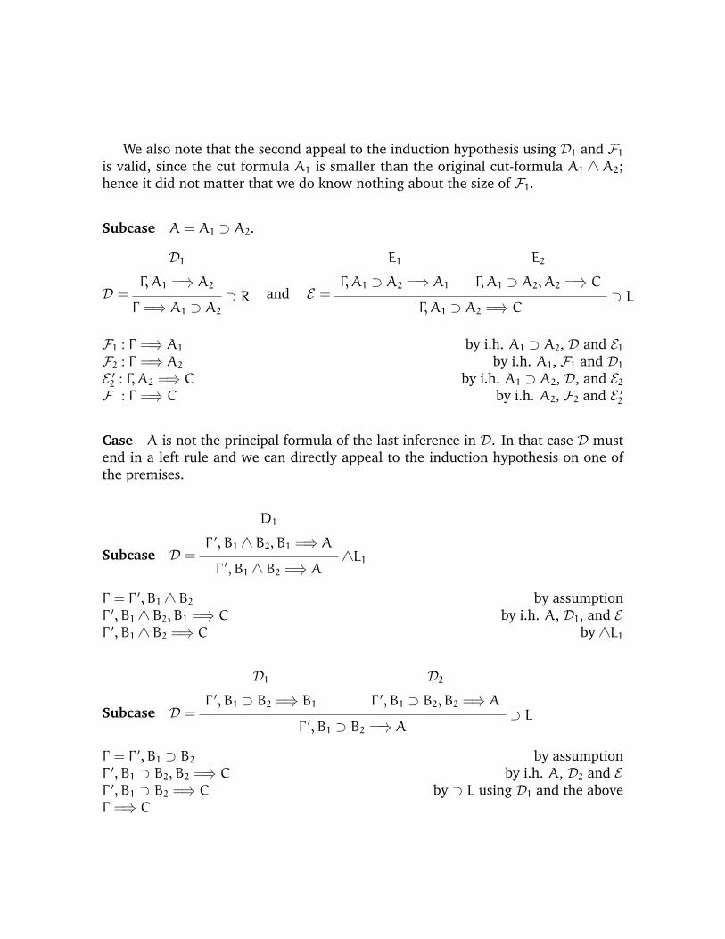
We also note that the second appeal to the induction hypothesis using D1 and F1is valid, since the cut formula A1 is smaller than the original cut-formula A1 ∧ A2;hence it did not matter that we do know nothing about the size of F1.

Subcase A = A1 ⊃ A2.

D =

D1Γ,A1 =⇒ A2

⊃ RΓ =⇒ A1 ⊃ A2

and E =

E1

Γ,A1 ⊃ A2 =⇒ A1

E2

Γ,A1 ⊃ A2, A2 =⇒ C⊃ L

Γ,A1 ⊃ A2 =⇒ C

F1 : Γ =⇒ A1 by i.h. A1 ⊃ A2, D and E1F2 : Γ =⇒ A2 by i.h. A1, F1 and D1E ′2 : Γ,A2 =⇒ C by i.h. A1 ⊃ A2, D, and E2F : Γ =⇒ C by i.h. A2, F2 and E ′2

Case A is not the principal formula of the last inference in D. In that case D mustend in a left rule and we can directly appeal to the induction hypothesis on one ofthe premises.

Subcase D =

D1

Γ ′, B1 ∧ B2, B1 =⇒ A∧L1

Γ ′, B1 ∧ B2 =⇒ A

Γ = Γ ′, B1 ∧ B2 by assumptionΓ ′, B1 ∧ B2, B1 =⇒ C by i.h. A, D1, and EΓ ′, B1 ∧ B2 =⇒ C by ∧L1

Subcase D =

D1Γ ′, B1 ⊃ B2 =⇒ B1

D2Γ ′, B1 ⊃ B2, B2 =⇒ A

⊃ LΓ ′, B1 ⊃ B2 =⇒ A

Γ = Γ ′, B1 ⊃ B2 by assumptionΓ ′, B1 ⊃ B2, B2 =⇒ C by i.h. A, D2 and EΓ ′, B1 ⊃ B2 =⇒ C by ⊃ L using D1 and the aboveΓ =⇒ C

Case A is not the principal formula of the last inference in E .

Subcase E =

E1Γ,A =⇒ C1

E2Γ,A =⇒ C2

∧RΓ,A =⇒ C1 ∧ C2

C = C1 ∧ C2 by assumptionΓ =⇒ C1 by i.h. A, D, and E1Γ =⇒ C2 by i.h. A, D, and E2ΓderC1 ∧ C2 by ∧R on the above

Subcase E =

E1Γ ′, B1 ∧ B2, B1, A =⇒ C

∧L1Γ ′, B1 ∧ B2, A =⇒ C

Γ = Γ ′, B1 ∧ B2 by assumptionΓ ′, B1 ∧ B2, B1 =⇒ C by i.h. A, D, E1Γ ′, B1 ∧ B2 =⇒ C by ∧L1Γ =⇒ C by Γ = Γ ′, B1 ∧ B2

As mentioned above, adding an admissible rule does not change the judgementswhich are derivable.

Theorem 5.1.11 (Cut Elimination).If Γ +

=⇒ C then Γ =⇒ C

Proof. By structural induction on the given derivation Γ +=⇒ C. The proof is straight-

forward, and we only write out the case for cut.

Case D+ =

D+1

Γ+

=⇒ A

D+2

Γ,A+

=⇒ ccut

Γ+

=⇒ C

Γ =⇒ A by i.h. on D+ + 1

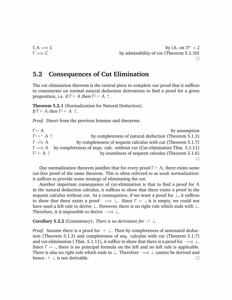
Γ,A =⇒ C by i.h. on D+ + 2Γ =⇒ C by admissibility of cut (Theorem 5.1.10)

5.2 Consequences of Cut Elimination

The cut elimination theorem is the central piece to complete our proof that it sufficesto concentrate on normal natural deduction derivations to find a proof for a givenproposition, i.e. if Γ ` A then Γ ↓ ` A ↑ .

Theorem 5.2.1 (Normalization for Natural Deduction).If Γ ` A then Γ ↓ ` A ↑ .

Proof. Direct from the previous lemmas and theorems.

Γ ` A by assumptionΓ ↓ `+ A ↑ by completeness of natural deduction (Theorem 5.1.3)Γ

+=⇒ A by completeness of sequent calculus with cut (Theorem 5.1.7)

Γ =⇒ A by completeness of sequ. calc. without cut (Cut-elimination Thm. 5.1.11)Γ ↓ ` A ↑ by soundness of sequent calculus (Theorem 5.1.6)

Our normalization theorem justifies that for every proof Γ ` A, there exists somecut-free proof of the same theorem. This is often referred to as weak normalization:it suffices to provide some strategy of eliminating the cut.

Another important consequence of cut-elimination is that to find a proof for Ain the natural deduction calculus, it suffices to show that there exists a proof in thesequent calculus without cut. As a consequence, if we want a proof for ⊥, it sufficesto show that there exists a proof · =⇒ ⊥. Since Γ = ·, it is empty, we could nothave used a left rule to derive ⊥. However, there is no right rule which ends with ⊥.Therefore, it is impossible to derive · =⇒ ⊥.

Corollary 5.2.2 (Consistency). There is no derivation for · ` ⊥.

Proof. Assume there is a proof for · ` ⊥. Then by completeness of annotated deduc-tion (Theorem 5.1.3) and completeness of seq. calculus with cut (Theorem 5.1.7)and cut-elimination ( Thm. 5.1.11), it suffice to show that there is a proof for · =⇒ ⊥.Since Γ = ·, there is no principal formula on the left and no left rule is applicable.There is also no right rule which ends in ⊥. Therefore · =⇒ ⊥ cannot be derived andhence · ` ⊥ is not derivable.

Another consequence, is that we can show that the excluded middle A ∨ ¬A isnot derivable. We also say that A∨ ¬A is independent for arbitrary A.

Corollary 5.2.3 (Independence of Excluded Middle).There is no deduction of ` A∨ ¬A for arbitrary A.

Proof. Assume there is a derivation ` A ∨ ¬A. By the completeness results and cut-elimination, it suffices to show · =⇒ A ∨ ¬A. By inversion, we must have either· =⇒ A or · =⇒ ¬A. The former judgement · =⇒ A has no derivation. The latterjudgement can only be inferred fromA =⇒ ⊥. But there is no right rule with the con-clusion ⊥ and we cannot prove given an arbitrary A we can derive a contradiction.Hence, there cannot be a deduction of ` A∨ ¬A.

Cut-elimination justifies that we can concentrate on finding a normal proof for aproposition A. We can also observe that proofs in the sequent calculus without cutare already much more restricted. Hence they are more amendable to proof search.The sequent calculus is hence an excellent foundation for proof search strategies.However, some non-determinism is still present. Should we apply a right rules or aleft rule? And if we choose to apply a left rule, which formula from Γ should we pickas our principal formula?

Without techniques to restrict some of these choices, proof search is still infea-sible. However, the sequent calculus lends itself to study these choices by consider-ing two important properties: inversion properties allow us apply rules eagerly, i.e.their order does not matter (don’t care non-determinism), and focusing propertiesallow us to chain rules which involve a choice and order does matter (do-care non-determinism), i.e. we make a choice we might as well continue to make choices andnot postpone them.

5.3 Towards a focused sequent calculus

The simplest way to avoid non-determinism is to consider those propositions on theleft or right for which a unique way to apply a rule. The following property essen-tially justifies that if we have the conclusion, then we must have had a proof of thepremises. For example, to prove A∧B, we can immediately apply the right rule with-out loosing completeness. On the other hand, to prove A∨B, we cannot immediatelyapply the right rule. As a counter example, consider B ∨ A =⇒ A ∨ B; we need toapply first the left rule for splitting the derivation and then apply the right rule.

Inversion property:The premises of an inference rule are derivable, if and only if the conclusion.

Given a sequent, a number of invertible rules may be applicable. However, theorder of this choice, i.e. when to apply an invertible rule, does not matter. In otherwords, we are replacing don’t know non-determinism by don’t care non-determinism.

For controlling and restricting the search space, we can refine the inversion prop-erty as stated above further. In particular, in left rules, the principal formula is stillpresent in the premises which means we can continue to apply the same left rule overand over again leading to non-termination. So we require in addition that the princi-pal formula of a left rule is no longer needed, thereby guaranteeing the terminationof the inversion phase.

Theorem 5.3.1 (Inversion).

1. If Γ =⇒ A∧ B then Γ =⇒ A and Γ =⇒ B

2. If Γ =⇒ A ⊃ B then Γ,A =⇒ B.

3. If Γ,A∧ B =⇒ C then Γ,A, B =⇒ C.

4. If Γ,A∨ B =⇒ C then Γ,A =⇒ C and Γ, B =⇒ C.

Proof. Proof by structural induction on the given derivation; or, simply taking advan-tage of cut.Γ =⇒ A∧ B by assumption

Γ,A∧ B,A =⇒ A by initΓ,A∧ B =⇒ A by ∧L1Γ =⇒ A by cut

We observe that >R and ⊥L are special; they can be applied eagerly, but theyhave no premises and therefore do not admit an inversion theorem.

There is a remarkable symmetry between the rules which are invertible and whichare not. This picture is slightly spoiled by the left rule for conjunction. This can becorrected in moving to linear logic which we will not pursue here.

Chaining all invertible rules together, already gives us a good proof search strat-egy. However, it still leaves us with many possible choices once we have applied allinvertible rules. How should one proceed to handle such choices? For example, if wepick a rule ∨R1 for (A∨ B)∨ C, we now need to prove A∨ B again facing a choice.Shall we stick to our committed choice and further split A ∨ B or shall we revisitother possible choices we have? - It turns out that focusing properties justify that wecan stick to a choice we have made and continue to make further choices.

Focusing properties are dual to inversion properties; while inversion propertiesallow us to chain together invertible rules, focusing properties allow us to chaintogether non-invertible rules committing to a choice.

The focusing property and the duality between invertible / non-invertible ruleswas first observed by Andreoli in linear logic which did not show the anomaly forconjunction. Following Andreoli, we can classify formulas into positive and negativepropositions where positive propositions are non-invertible on the right, but invertibleon the left and negative propositions are non-invertible on the left, but invertible onthe right.

Formula A,B ::= R | L

Positive R ::= P+ | A1 ∨A2 | ∃x:τ.A(x) | ⊥ | A1 ∧A2Negative L ::= P− | A1 ⊃ A2 | ∀x:τ.A(x) | A1 ∧A2Stable Context ∆ ::= · | ∆, L

Moreover, we will describe a stable context ∆ which only consists of negativeformulas. Intuitively, we will first consider first a formulaA and apply invertible ruleson the right until we obtain a positive proposition; at this point, we shift our attentionto the context of assumptions and apply invertible left rules until our context is stable,i.e. it contains only negative propositions. At this point we have to make a choice.This phase is called the asynchronous phase.

From the asynchronous phase, we transition to the synchronous phase. We eithercommit to work on the right hand side of the sequent (∆ > R) or we commit to workon the left hand side choosing an assumption from ∆, i.e. ∆ > L =⇒ R. Let ussummarize the four judgements:

∆; Γ =⇒ [L] Asynchronous phase (right)∆; [Γ ] =⇒ R Asynchronous phase (left)∆ > R Synchronous phase (right)∆ > L =⇒ R Synchronous phase (left)

The notation ∆ > R and ∆ > L =⇒ R is chosen to draw attention to the partwe focus on via >; the left hand side of > describes the narrowing the focus of ourattention.

Synchronous phase (left)

∆ > A ∆ > B =⇒ R

∆ > A ⊃ B =⇒ R

∆ > A(t) =⇒ R

∆ > ∀x.A(x) =⇒ R

∆ > Ai =⇒ R

∆ > A1 ∧A2 =⇒ R

Asynchronous phase (right)

∆; Γ,A =⇒ [ B ]

∆; Γ =⇒ [ A ⊃ B ]

∆; Γ =⇒ [ A(a) ]

∆; Γ =⇒ [ ∀x.A(x) ]

∆; Γ =⇒ [ A ] ∆; Γ =⇒ [ B ]

∆; Γ =⇒ [ A∧ B ]

Asynchronous phase (left)

∆; [ Γ,A(a) ] =⇒ R

∆; [ Γ,∃x.A(x) ] =⇒ R

∆; [ Γ,A ] =⇒ R ∆; [ Γ, B ] =⇒ R

∆; [ Γ,A∨ B ] =⇒ R

∆; [ Γ,A, B ] =⇒ R

∆; [ Γ,A∧ B ] =⇒ R

Synchronous phase (right)

∆ > A(t)

∆ > ∃x.A(x)

∆ > Ai

∆ > A1 ∨A2

∆ > A1 ∆ > A2

∆ > A1 ∧A2

Identity (positive) Identity (negative)

∆, P > P+ ∆ > P =⇒ P−

Transition rules

L ∈ ∆ ∆ > L =⇒ RchoiceL

∆; [ · ] =⇒ R

∆ > RchoiceR

∆; [ · ] =⇒ R

∆; · =⇒ [ L ]BlurR

∆ > L

∆; [ R ] =⇒ R ′

BlurL∆ > R =⇒ R ′

∆, L; [ Γ ] =⇒ RMove-to-stable-context

∆; [ Γ, L ] =⇒ R

∆; [ Γ ] =⇒ RTransition-to-left

∆; Γ =⇒ [ R ]

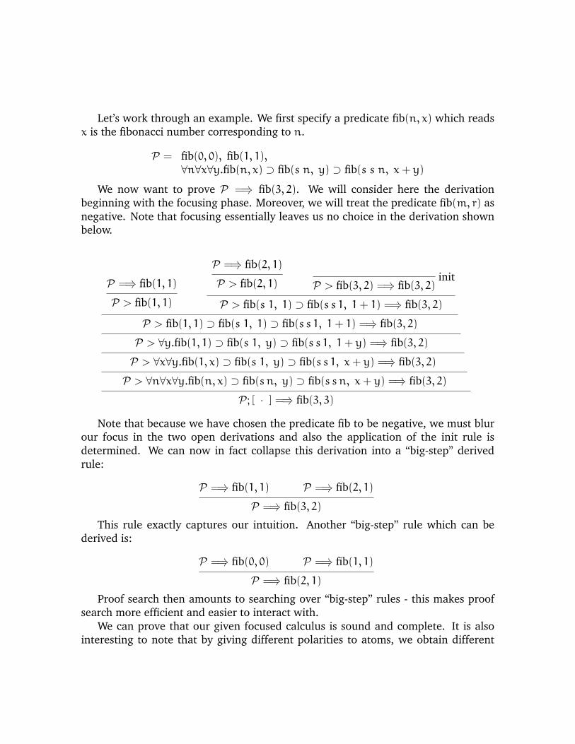
Let’s work through an example. We first specify a predicate fib(n, x) which readsx is the fibonacci number corresponding to n.

P = fib(0, 0), fib(1, 1),∀n∀x∀y.fib(n, x) ⊃ fib(s n, y) ⊃ fib(s s n, x+ y)

We now want to prove P =⇒ fib(3, 2). We will consider here the derivationbeginning with the focusing phase. Moreover, we will treat the predicate fib(m, r) asnegative. Note that focusing essentially leaves us no choice in the derivation shownbelow.

P =⇒ fib(1, 1)

P > fib(1, 1)

P =⇒ fib(2, 1)

P > fib(2, 1) initP > fib(3, 2) =⇒ fib(3, 2)

P > fib(s 1, 1) ⊃ fib(s s 1, 1+ 1) =⇒ fib(3, 2)

P > fib(1, 1) ⊃ fib(s 1, 1) ⊃ fib(s s 1, 1+ 1) =⇒ fib(3, 2)

P > ∀y.fib(1, 1) ⊃ fib(s 1, y) ⊃ fib(s s 1, 1+ y) =⇒ fib(3, 2)

P > ∀x∀y.fib(1, x) ⊃ fib(s 1, y) ⊃ fib(s s 1, x+ y) =⇒ fib(3, 2)

P > ∀n∀x∀y.fib(n, x) ⊃ fib(sn, y) ⊃ fib(s sn, x+ y) =⇒ fib(3, 2)

P ; [ · ] =⇒ fib(3, 3)

Note that because we have chosen the predicate fib to be negative, we must blurour focus in the two open derivations and also the application of the init rule isdetermined. We can now in fact collapse this derivation into a “big-step” derivedrule:

P =⇒ fib(1, 1) P =⇒ fib(2, 1)

P =⇒ fib(3, 2)

This rule exactly captures our intuition. Another “big-step” rule which can bederived is:

P =⇒ fib(0, 0) P =⇒ fib(1, 1)

P =⇒ fib(2, 1)

Proof search then amounts to searching over “big-step” rules - this makes proofsearch more efficient and easier to interact with.

We can prove that our given focused calculus is sound and complete. It is alsointeresting to note that by giving different polarities to atoms, we obtain different

proof search strategies - assigning negative polarities to atoms allows us to modelbackwards proof search as we have illustrated; assigning positive polarities to atomsin fact leads to forward proof search. Hence the system is general enough to modeldifferent proof search strategies. This was observed by Chaudhuri and Pfenning.

Moreover, it is worth noting that we can give it a computational interpretations;focusing calculi provide a type system for languages supporting pattern matchingand different proof strategies correspond to different evaluation strategies modellingcall-by-value or call-by-name evaluation (see for example work by Noam Zeilberger).

Chapter 6

Normalization

We discuss here an alternative proof method for proving normalization. We will focushere on a semantic proof method using saturated sets. This proof method goes backto Girard (1972) building on some previous ideas by Tait.

The key question is how to prove that give a lambda-term, its evaluation termi-nates, i.e. normalizes. Recall the lambda-calculus together with its reduction rules.

Terms M,N ::= x | λx.M |MN

We consider as the main rule for reduction (or evaluation) applying a term to anabstraction, called β-reduction.

(λx.M) N −→ [N/x]M β-reduction

The β-reduction rule only applies once we have found a redex. However, we alsoneed congruence rules to allow evaluation of arbitrary subterms.

M −→M ′

MN −→M ′NN −→ N ′

MN −→MN ′M −→M ′

λx.M −→ λx.M ′

The question then is, how do we know that reducing a well-typed lambda-termwill halt? - This is equivalent to asking does a well-typed lambda-term normalize, i.e.after some reduction steps we will end up in a normal form where there are no fur-ther reductions possible. Since a normal lambda-term characterizes normal proofs,normalizing a lambda-term corresponds to normalizing proofs and demonstrates thatevery proof in the natural deduction system indeed has a normal proof.

Proving that reduction must terminate is not a simple syntactic argument basedon terms, since the β-reduction rule may yield a term which is bigger than the termwe started with. We hence need to find a different inductive argument. For thesimply-typed lambda-calculus, we can prove that while the expression itself does not

81

get smaller, the type of an expression is. This is a syntactic argument; it however doesnot scale to polymorphic lambda-calculus. We will here instead discuss a semanticproof method where we define the meaning of well-typed terms using the abstractnotion of reducibility candidates.

6.1 General idea

We can define the meaning of a well-typed term M in the context Γ of type A asfollows: for all grounding instantiations σ providing values for the variables declaredin Γ , [σ]M is in the denotation of A. We write for the denotation of A as [[A]] = A.Similarly, the denotation of Γ is written as [[Γ ]] = G.

[[A]] is interpreted as the sets of strongly normalizing terms of type A, i.e. [[A]] ∈SN. We prove that if a term is well-typed, then it is strongly normalizing in two steps:

Step 1 If M ∈ [[A]] then M ∈ SN.

Step 2 If Γ `M : A and σ ∈ [[Γ ]] then [σ]M ∈ [[A]].

Therefore, we can conclude that if a term M has type A then M ∈ SN, i.e. M isstrongly normalizing and its reduction is finite, choosing σ to be the identity substi-tution.

We remark first, that all variables are in the denotations of a type A, i.e. Var ⊆ [[A]],and variables are strongly normalizing, i.e. they are already in normal form.

Next, we define the denotations of the base type o and the function type A→ B.

• A term M ∈ [[o]] iff M is strongly normalizing, i.e. M ∈ SN.

• A term M ∈ [[A→ B]] iff M ∈ [[A]] =⇒ [[B]], i.e. for all N ∈ [[A]].M N ∈ [[B]].

We often write these definitions more compactly as follows

Semantic base type [[o]] := SNSemantic function type [[A→ B]] := {M|∀N ∈ [[A]].M N ∈ [[B]]}

6.2 Defining strongly normalizing terms

Intuitively, a term M is strongly normalizing, if there exists no infinite reductionsequence. Constructively, we can define strong normalization as follows:

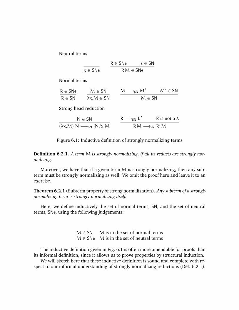
Neutral terms

x ∈ SNe

R ∈ SNe s ∈ SN

RM ∈ SNe

Normal terms

R ∈ SNe

R ∈ SN

M ∈ SN

λx.M ∈ SN

M −→SN M′ M ′ ∈ SN

M ∈ SN

Strong head reduction

N ∈ SN

(λx.M) N −→SN [N/x]M

R −→SN R′ R is not a λ

RM −→SN R′M

Figure 6.1: Inductive definition of strongly normalizing terms

Definition 6.2.1. A term M is strongly normalizing, if all its reducts are strongly nor-malizing.

Moreover, we have that if a given term M is strongly normalizing, then any sub-term must be strongly normalizing as well. We omit the proof here and leave it to anexercise.

Theorem 6.2.1 (Subterm property of strong normalization). Any subterm of a stronglynormalizing term is strongly normalizing itself.

Here, we define inductively the set of normal terms, SN, and the set of neutralterms, SNe, using the following judgements:

M ∈ SN M is in the set of normal termsM ∈ SNe M is in the set of neutral terms

The inductive definition given in Fig. 6.1 is often more amendable for proofs thanits informal definition, since it allows us to prove properties by structural induction.

We will sketch here that these inductive definition is sound and complete with re-spect to our informal understanding of strongly normalizing reductions (Def. 6.2.1).

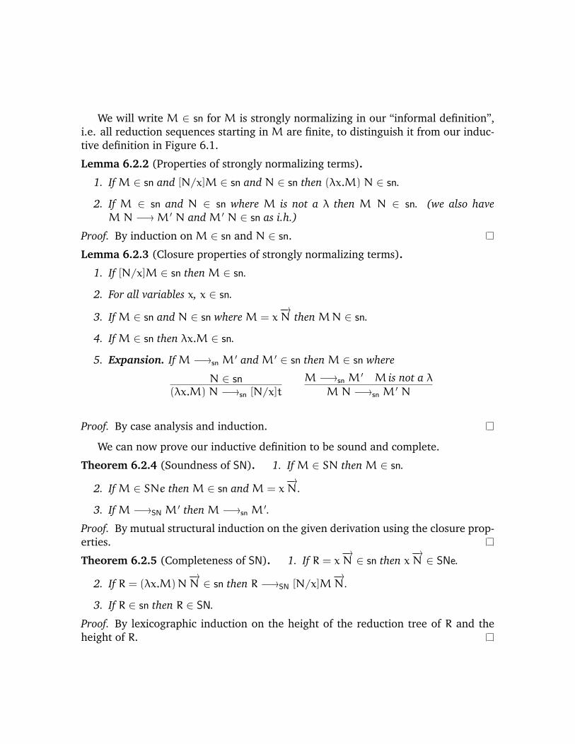
We will write M ∈ sn for M is strongly normalizing in our “informal definition”,i.e. all reduction sequences starting in M are finite, to distinguish it from our induc-tive definition in Figure 6.1.

Lemma 6.2.2 (Properties of strongly normalizing terms).

1. If M ∈ sn and [N/x]M ∈ sn and N ∈ sn then (λx.M) N ∈ sn.

2. If M ∈ sn and N ∈ sn where M is not a λ then M N ∈ sn. (we also haveMN −→M ′ N and M ′ N ∈ sn as i.h.)

Proof. By induction on M ∈ sn and N ∈ sn.

Lemma 6.2.3 (Closure properties of strongly normalizing terms).

1. If [N/x]M ∈ sn then M ∈ sn.

2. For all variables x, x ∈ sn.

3. If M ∈ sn and N ∈ sn where M = x−→N then MN ∈ sn.

4. If M ∈ sn then λx.M ∈ sn.

5. Expansion. If M −→sn M′ and M ′ ∈ sn then M ∈ sn where

N ∈ sn(λx.M) N −→sn [N/x]t

M −→sn M′ M is not a λ

M N −→sn M′ N

Proof. By case analysis and induction.

We can now prove our inductive definition to be sound and complete.

Theorem 6.2.4 (Soundness of SN). 1. If M ∈ SN then M ∈ sn.

2. If M ∈ SNe then M ∈ sn and M = x−→N .

3. If M −→SN M′ then M −→sn M

′.

Proof. By mutual structural induction on the given derivation using the closure prop-erties.

Theorem 6.2.5 (Completeness of SN). 1. If R = x−→N ∈ sn then x

−→N ∈ SNe.

2. If R = (λx.M)N−→N ∈ sn then R −→SN [N/x]M

−→N .

3. If R ∈ sn then R ∈ SN.

Proof. By lexicographic induction on the height of the reduction tree of R and theheight of R.

6.3 Reducibility Candidates

One might ask, what is a good definition of a semantic type? - Rather than attemptingthe proof of the fundamental lemma directly and then trying to extract additionallemmas one might need about the semantic types, we follow Girard’s technique andcharacterize some key properties our semantic types need to satisfy. If a semantictype satisfies these key properties, then our proof of the fundamental lemma will bestraightforward. To put it differently, defining these key properties, will allow for a amodular proof of the fundamental lemma.

Definition 6.3.1 (Reducibility Candidate). A set [[A]] is a reducibility candidate, [[A]] ∈CR if the following conditions hold

• CR1 : If M ∈ [[A]] then M ∈ SN, i.e. [[A]] ⊆ SN.

• CR2 : If M ∈ SNe then M ∈ [[A]], i.e. SNe ⊆ [[A]].

• CR3 :M −→SN M

′ M ′ ∈ [[A]]

M ∈ [[A]], i.e. [[A]] is closed under reduction.

The last property is often also referred to as backward closed. We show that thatall semantic types [[A]] satisfy the conditions above.

Theorem 6.3.1. For all types C, [[C]] ∈ CR.

Proof. By induction on the structure of A. We highlight the cases below.

Case: C = o .

1. Show CR1: By definition, for all M ∈ [[o]], we have that M ∈ SN.

2. Show CR2: By assumption M ∈ SNe. By the definition of SN, we thereforeknow M ∈ SN; by definition of [[o]], M ∈ [[o]].

3. Show CR3: Trivially true, since there is no step we can take with −→SN.

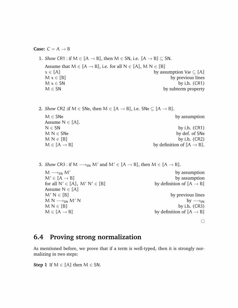
Case: C = A→ B

1. Show CR1 : if M ∈ [[A→ B]], then M ∈ SN, i.e. [[A→ B]] ⊆ SN.

Assume that M ∈ [[A→ B]], i.e. for all N ∈ [[A]], MN ∈ [[B]]x ∈ [[A]] by assumption Var ⊆ [[A]]M x ∈ [[B]] by previous linesM x ∈ SN by i.h. (CR1)M ∈ SN by subterm property

2. Show CR2 :if M ∈ SNe, then M ∈ [[A→ B]], i.e. SNe ⊆ [[A→ B]].

M ∈ SNe by assumptionAssume N ∈ [[A]].N ∈ SN by i.h. (CR1)MN ∈ SNe by def. of SNeMN ∈ [[B]] by i.h. (CR2)M ∈ [[A→ B]] by definition of [[A→ B]].

3. Show CR3 : if M −→SN M′ and M ′ ∈ [[A→ B]], then M ∈ [[A→ B]].

M −→SN M′ by assumption

M ′ ∈ [[A→ B]] by assumptionfor all N ′ ∈ [[A]], M ′ N ′ ∈ [[B]] by definition of [[A→ B]]Assume N ∈ [[A]]M ′ N ∈ [[B]] by previous linesMN −→SN M

′ N by −→SN

MN ∈ [[B]] by i.h. (CR3)M ∈ [[A→ B]] by definition of [[A→ B]]

6.4 Proving strong normalization

As mentioned before, we prove that if a term is well-typed, then it is strongly nor-malizing in two steps:

Step 1 If M ∈ [[A]] then M ∈ SN.

Step 2 If Γ `M : A and σ ∈ [[Γ ]] then [σ]M ∈ [[A]].

The first part described in Step 1, is satisfied by the fact that [[A]] must be areducibility candidate. Hence by CR1 all terms in [[A]] are strongly normalizing. Wenow prove the second step, which is often referred to as the Fundamental Lemma. Itstates that ifM has typeA and we can provide “good” instantiation σ, which providesterms which are themselves normalizing for all the free variables in M, then [σ]M isin [[A]].

Lemma 6.4.1 (Fundamental lemma). If Γ `M : A and σ ∈ [[Γ ]] then [σ]M ∈ [[A]].

Proof. By induction on Γ `M : A.

Case D =Γ(x) = A

Γ ` x : A

σ ∈ [[Γ ]] by assumption[σ]x ∈ [[Γ(x)]] = [[A]] by definition

Case D = Γ `M : A→ B Γ ` N : A

Γ `MN : Bσ ∈ [[Γ ]] by assumption[σ]M ∈ [[A→ B]] by i.h.for all N ′ ∈ [[A]]. ([σ]M) N ′ ∈ [[B]] by definition of [[A→ B]][σ]N ∈ [[A]] by i.h.[σ]M [σ]N ∈ [[B]] by previous lines[σ](MN) ∈ [[B]] by subst. definition

Case D = Γ, x : A `M : B

Γ ` λx.M : A→ Bσ ∈ [[Γ ]] by assumptionAssume N ∈ [[A]](σ,N/x) ∈ [[Γ, x : A]] by definition[σ,N/x]M ∈ [[B]] by i.h.(λx.[σ, x/x]M) N −→SN [σ,N/x]M by reduction −→SN

(λx.[σ, x/x]M) = [σ](λx.M) by subst. def([σ]λx.M) N ∈ [[B]] by CR3for all N ∈ [[A]]. ([σ]λx.M) N ∈ [[B]] by previous lines[σ](λx.M) ∈ [[A→ B]] by definition of [[A→ B]]

Neutral termsM ∈ SNe N1 ∈ SN N2 ∈ SN

caseM of inl x⇒ N1 | inry⇒ N2 ∈ SNeNormal terms

M ∈ SNinl M ∈ SN

M ∈ SNinr M ∈ SN

Strong head reduction

M ∈ SN N2 ∈ SN

case (inl M) of inl x⇒ N1 | inry⇒ N2 −→SN [M/x]N1

M ∈ SN N1 ∈ SN

case (inr M) of inl x⇒ N1 | inry⇒ N2 −→SN [M/x]N2

M −→SN M′

caseM of inl x⇒ N1 | inry⇒ N2 −→SN caseM ′ of inl x⇒ N1 | inry⇒ N2

Figure 6.2: Inductive definition of strongly normalizing terms - extended for case-expressions and injections

Corollary 6.4.2. If Γ `M : A then M ∈ SN.

Proof. Using the fundamental lemma with the identity substitution id ∈ [[Γ ]], we ob-tain M ∈ [[A]]. By CR1, we know M ∈ SN.

6.5 Extension: Disjoint sums

We will now extend our simply-typed lambda-calculus to disjoint sums.

Types A ::= . . . | A+ BTerms M ::= . . . | inl M | inr M | caseM of inl x⇒ N1 | inry⇒ N2

Let us first extend our definition of SN and SNe (see Fig. 6.2).Next, we extend our definition of semantic type to disjoint sums. A first attempt

might be to define [[A+ B]] as follows

Attempt 1

[[A+ B]] := {inl M |M ∈ [[A]]} ∪ {inr M |M ∈ [[B]]}

However, this definition would not satisfy the key property CR3 and hence wouldfail to be a reducibility candidate. For example, while inl y is in [[A + B]], (λx.inl x) ywould not be in [[A+ B]] despite the fact that (λx.inl x) y −→SN inl y.

Our definition of [[A + B]] is not closed under the reduction relation −→SN. Let Adenote the denotation of [[A]]. We then define the closure of [[A]] = A, written as A,inductively as follows:

M ∈ AM ∈ A

M ∈ SNe

M ∈ A

M ∈ A N −→SN M

N ∈ Aand we define

[[A+ B]] = {inl M |M ∈ [[A]]} ∪ {inr M |M ∈ [[B]]}

6.5.1 Semantic type [[A+ B]] is a reducibility candidate

We first extend our previous theorem which states that all denotations of types mustbe in CR.

Theorem 6.5.1. For all types C, [[C]] ∈ CR.

Proof. By induction on the structure of A. We highlight the case for disjoint sums.

Case C = A+ B.

1. Show CR1. Assume thatM ∈ [[A+B]]. We consider different subcases and proveby an induction on the closure defining [[A+ B]] that M ∈ SN.

Subcase: M ∈ {inl N | N ∈ [[A]]} . Therefore M = inl N. Since N ∈ [[A]] andby i.h. (CR1), N ∈ SN. By definition of SN, we have that inl N ∈ SN.

Subcase: M ∈ {inr N | N ∈ [[B]]} . Therefore M = inr N. Since N ∈ [[B]] andby i.h. (CR1), N ∈ SN. By definition of SN, we have that inr N ∈ SN.

Subcase: M ∈ SNe . By definition of SN, we conclude that M ∈ SN.

Subcase: M ∈ [[A+ B]], if M −→SN M′ and M ′ ∈ [[A+ B]] .

M −→SN M′ and M ′ ∈ [[A+ B]] by assumption

M ′ ∈ SN by inner i.h.M ∈ SN by reduction −→SN

2. Show CR2.if M ∈ SNe, then M ∈ [[A+ B]]By definition of the closure, if M ∈ SNe, we have M ∈ [[A+ B]].

3. Show CR3. if M −→SN M′ and M ′ ∈ [[A+ B]] then M ∈ [[A+ B]].

By definition of the closure, if M −→SN M′ and M ′ ∈ [[A + B]], we have M ∈

[[A+ B]].

6.5.2 Revisiting the fundamental lemma

We can now revisit the fundamental lemma.

Lemma 6.5.2 (Fundamental lemma). If Γ `M : A and σ ∈ [[Γ ]] then [σ]M ∈ [[A]].

Proof. By induction on Γ `M : A.

Case D =Γ `M : A+ B Γ, x:A ` N1 : C Γ, y:B ` N2 : C

Γ ` caseM of inl x⇒ N1 | inry⇒ N2 : C

σ ∈ [[Γ ]] by assumption[σ]M ∈ [[A+ B]] by i.h.

We consider different subcases and prove by induction on the closure defining [[A +B]], that [σ](caseM of inl x⇒M1 | inry⇒M2) ∈ [[C]].

Subcase [σ]M ∈ {inl N | N ∈ [[A]]}

[σ]M = inl N for some N ∈ [[A]] by assumptionN ∈ SN by CR1σ ∈ [[Γ ]] by assumption[σ,N/x] ∈ [[Γ, x : A]] by definition[σ,N/x]M1 ∈ [[C]] by outer i.h.y ∈ [[B]] by definition[σ, y/y] ∈ [[Γ, y : B]] by definition

[σ, y/y]M2 ∈ [[C]] by outer i.h.[σ, y/y]M2 ∈ SN by CR1case (inl N) of inl x⇒ [σ, x/x]M1 | inry⇒ [σ, y/y]M2 −→SN [σ,N/x]M1 by −→SN

case (inl N) of inl x⇒ [σ, x/x]M1 | inry⇒ [σ, y/y]M2

= [σ](caseM of inl x⇒M1 | inry⇒M2) by subst. definition and [σ]M = inl N[σ](caseM of inl x⇒M1 | inry⇒M2) ∈ [[C]] by CR3

Subcase [σ]M ∈ {inr N | N ∈ [[B]]}

similar to the case above.

Subcase: [σ]M ∈ SNe .σ ∈ Γ by assumptionx ∈ [[A]], y ∈ [[B]] by definition[σ, y/y] ∈ [[Γ, y : B]] by definition[σ, x/x] ∈ [[Γ, x : A]] by definition[σ, x/x]M1 ∈ [[C]] by outer i.h.[σ, y/y]M2 ∈ [[C]] by outer i.h.[σ, y/y]M2 ∈ SN by CR1[σ, x/x]M1 ∈ SN by CR1case [σ]M of inl x⇒ [σ, x/x]M1 | inry⇒ [σ, y/y]M2 ∈ SNe by SNe[σ](caseM of inl x⇒M1 | inry⇒M2) ∈ SNe by substitution def.[σ](caseM of inl x⇒M1 | inry⇒M2) ∈ [[C]] by CR2

Subcase: [σ]M ∈ [[A+ B]], if [σ]M −→SN M′ and M ′ ∈ [[A+ B]]

[σ]M −→SN M′ and M ′ ∈ [[A+ B]] by assumption

caseM ′ of inl x⇒ [σ, x/x]M1 | inry⇒ [σ, y/y]M2 ∈ [[C]] by inner i.h.case [σ]M of inl x⇒ [σ, x/x]M1 | inry⇒ [σ, y/y]M2

−→SN caseM ′ of inl x⇒ [σ, x/x]M1 | inry⇒ [σ, y/y]M2 by −→SN

[σ](caseM of inl x⇒M1 | inry⇒M2) ∈ [[C]] by CR3

6.6 Extension: Recursion

We now extend our simply-typed lambda-calculus to include natural numbers definedby z and suc t as well as a primitive recursion operator written as rec M with f z →Mz | f (sucn) → Ms where M is the argument we recurse over, Mz describes thebranch taken if M = z and Ms describes the branch taken when M = sucN where nwill be instantiated with N and f n describes the recursive call.

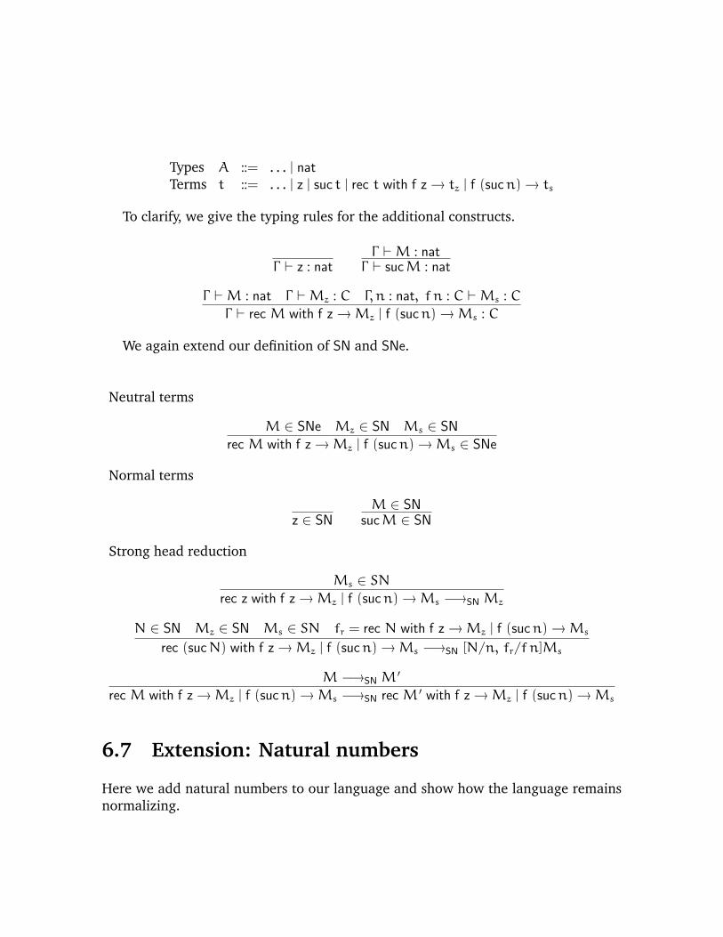
Types A ::= . . . | natTerms t ::= . . . | z | suc t | rec t with f z → tz | f (sucn) → ts

To clarify, we give the typing rules for the additional constructs.

Γ ` z : natΓ `M : natΓ ` sucM : nat

Γ `M : nat Γ `Mz : C Γ, n : nat, f n : C `Ms : C

Γ ` rec M with f z →Mz | f (sucn) →Ms : C

We again extend our definition of SN and SNe.

Neutral terms

M ∈ SNe Mz ∈ SN Ms ∈ SN

rec M with f z →Mz | f (sucn) →Ms ∈ SNe

Normal terms

z ∈ SNM ∈ SN

sucM ∈ SN

Strong head reduction

Ms ∈ SNrec z with f z →Mz | f (sucn) →Ms −→SN Mz

N ∈ SN Mz ∈ SN Ms ∈ SN fr = rec N with f z →Mz | f (sucn) →Ms

rec (sucN) with f z →Mz | f (sucn) →Ms −→SN [N/n, fr/fn]Ms

M −→SN M′

rec M with f z →Mz | f (sucn) →Ms −→SN rec M ′ with f z →Mz | f (sucn) →Ms

6.7 Extension: Natural numbers

Here we add natural numbers to our language and show how the language remainsnormalizing.

6.7.1 Semantic type [[nat]]

We define the denotation of nat as follows:

[[nat]] := {z} ∪ {sucM |M ∈ [[nat]]}

6.7.2 Semantic type [[nat]] is a reducibility candidate

We again extend our previous theorem which states that all denotations of types mustbe in CR.

Theorem 6.7.1. For all types C, [[C]] ∈ CR.

Proof. By induction on the structure of A. We highlight the case for nat.

Case C = nat

1. Show CR1: Assume M ∈ nat. we consider different subcases and prove byinduction on the closure defining nat that M ∈ SN.

Subcase M = z. By definition of SN, z ∈ SN.

Subcase M = sucN where N ∈ [[nat]]. By i.h. (CR1), N ∈ SN. By definitionof SN, sucN ∈ SN.

Subcase M ∈ SNe. By definition of SN, M ∈ SN.

Subcase M ∈ [[nat]], if M −→SN M′ and M ′ ∈ [[nat]].

M −→SN M′ and M ′ ∈ [[nat]] by assumption

M ′ ∈ SN by inner i.h.M ∈ SN by reduction −→SN

Show CR2: By definition of the closure, M ∈ SNe, then M ∈ [[nat]].

Show CR3: M ∈ nat, if M −→SN M′ and M ′ ∈ nat. By definition of the closure, we

have that M ∈ nat.

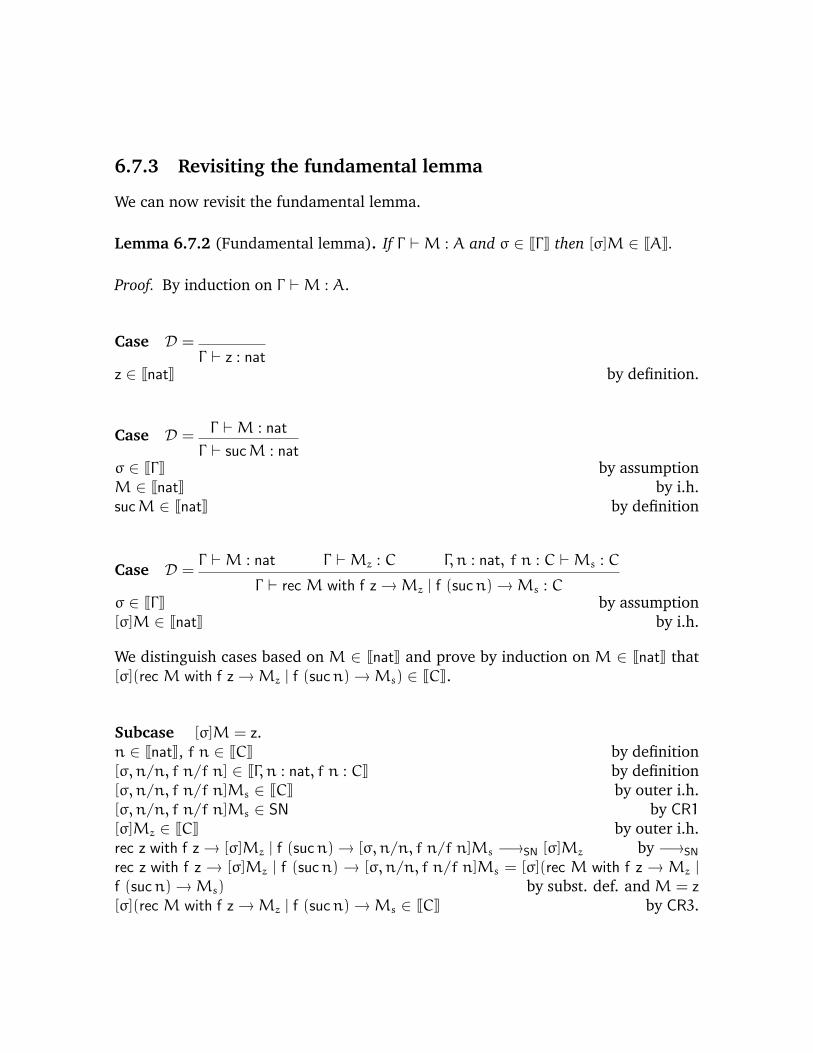
6.7.3 Revisiting the fundamental lemma

We can now revisit the fundamental lemma.

Lemma 6.7.2 (Fundamental lemma). If Γ `M : A and σ ∈ [[Γ ]] then [σ]M ∈ [[A]].

Proof. By induction on Γ `M : A.

Case D =Γ ` z : nat

z ∈ [[nat]] by definition.

Case D = Γ `M : nat

Γ ` sucM : natσ ∈ [[Γ ]] by assumptionM ∈ [[nat]] by i.h.sucM ∈ [[nat]] by definition

Case D =Γ `M : nat Γ `Mz : C Γ, n : nat, f n : C `Ms : C

Γ ` rec M with f z →Mz | f (sucn) →Ms : Cσ ∈ [[Γ ]] by assumption[σ]M ∈ [[nat]] by i.h.

We distinguish cases based on M ∈ [[nat]] and prove by induction on M ∈ [[nat]] that[σ](rec M with f z →Mz | f (sucn) →Ms) ∈ [[C]].

Subcase [σ]M = z.n ∈ [[nat]], f n ∈ [[C]] by definition[σ, n/n, f n/f n] ∈ [[Γ, n : nat, f n : C]] by definition[σ, n/n, f n/f n]Ms ∈ [[C]] by outer i.h.[σ, n/n, f n/f n]Ms ∈ SN by CR1[σ]Mz ∈ [[C]] by outer i.h.rec z with f z → [σ]Mz | f (sucn) → [σ, n/n, f n/f n]Ms −→SN [σ]Mz by −→SN

rec z with f z → [σ]Mz | f (sucn) → [σ, n/n, f n/f n]Ms = [σ](rec M with f z → Mz |

f (sucn) →Ms) by subst. def. and M = z[σ](rec M with f z →Mz | f (sucn) →Ms ∈ [[C]] by CR3.

Subcase [σ]M = sucM ′ where M ′ ∈ [[nat]].M ′ ∈ [[nat]] by assumptionM ′ ∈ SN by CR1[σ]Mz ∈ [[C]] by outer i.h.[σ]Mz ∈ SN by CR1[σ, n/n, f n/f n]Ms ∈ [[C]] by outer i.h.[σ, n/n, f n/f n]Ms ∈ SN by CR1rec M ′ with f z → [σ]Mz | f (sucn) → [σ, n/n, f n/f n]Ms ∈ [[C]] by inner i.h.[σ,M ′/x, rec M ′ with f z → [σ]Mz | f (sucn) → [σ, n/n, f n/f n]Ms/f n] ∈ [[Γ, n :nat, f n : C]] by definition[σ,M ′/x, rec M ′ with f z → [σ]Mz | f (sucn) → [σ, n/n, f n/f n]Ms/f n]Ms ∈ [[C]] byouter i.h.rec (sucM ′) with f z → [σ]Mz | f (sucn) → [σ, n/n, f n/f n]Ms

−→SN [σ,M ′/x, rec M ′ with f z → [σ]Mz | f (sucn) → [σ, n/n, f n/f n]Ms/f n]Ms

by −→SN

[σ](rec M with f z →Mz | f (sucn) →Ms) ∈ [[C]] by CR3.

Subcase [σ]M ∈ SNe.[σ]Mz ∈ [[C]] by outer i.h.[σ]Mz ∈ SN by CR1[σ, n/n, f n/f n]Ms ∈ [[C]] by outer i.h.[σ, n/n, f n/f n]Ms ∈ SN by CR1rec [σ]M with f z → [σ]Mz | f (sucn) → [σ, n/n, f n/f n]Ms ∈ SNe by SNe[σ](rec M with f z →Mz | f (sucn) →Ms) ∈ SNe by subst. def.[σ](rec M with f z →Mz | f (sucn) →Ms) ∈ [[C]] by CR2.

Subcase [σ]M ∈ [[nat]], if [σ]M −→SN M′ and M ′ ∈ [[nat]].

[σ]M −→SN M′ and M ′ ∈ [[nat]] by assumption.

rec M ′ with f z → [σ]Mz | f (sucn) → [σ, n/n, f n/f n]Ms ∈ [[C]] by inner i.h.rec [σ]M with f z → [σ]Mz | f (sucn) → [σ, n/n, f n/f n]Ms

−→SN rec M ′ with f z → [σ]Mz | f (sucn) → [σ, n/n, f n/f n]Ms by −→SN

[σ](rec M with f z →Mz | f (sucn) →Ms) ∈ [[C]] by CR3.

Bibliography

[Belnap(1962)] Nuel D. Belnap. Tonk, plonk, and plink. Analysis, 22(6):130–134,1962.

[Dummett(1993)] Michael Dummett. The Logical Basis of Metaphysics. Harvard Uni-versity Press, Cambridge, Massachusetts, 1993.

[Gentzen(1935)] Gerhard Gentzen. Untersuchungen uber das logische Schließen.Mathematische Zeitschrift, 39:176–210, 1935.

97