Logic Synthesis

• Minimization of Boolean logic– Technology-independent mapping

• Objective: minimize # of implicants, # of literals, etc.

• Not directly related to precise technology (# transistors), but correlated – consistent with objectives for any technology

– Technology-dependent mapping• Linked to precise technology/library

• Technology-independent mapping– Two-level minimization – sum of products (SOP)/product of sums (POS)

• Karnaugh maps – “visual” technique

• Quine-McCluskey method – algorithmic

• Heuristic minimization – fast and “pretty good,” but not exact

– Multi-level minimization

Basic Definitions

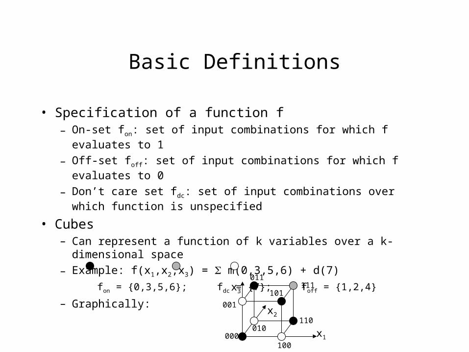
• Specification of a function f– On-set fon: set of input combinations for which f evaluates to 1

– Off-set foff: set of input combinations for which f evaluates to 0

– Don’t care set fdc: set of input combinations over which function is unspecified

• Cubes– Can represent a function of k variables over a k-dimensional space

– Example: f(x1,x2,x3) = m(0,3,5,6) + d(7)

fon = {0,3,5,6}; fdc = {7}; foff = {1,2,4}

– Graphically:

x1

x2

x3

000

110

100

001

101111

011

010

k-cubes

• k-cube: k-dim. subset of fon

– 0-cube = vertex in fon

– k-cube = a pair of (k-1) cubes with a Hamming distance of 1

• Examples– A 0-cube is a vertex

– A 1-cube is an edge

– A 2-cube is a face

– A 3-cube is a 3D cube

– A 4-cube is harder to visualize but can be shown as

More defintions

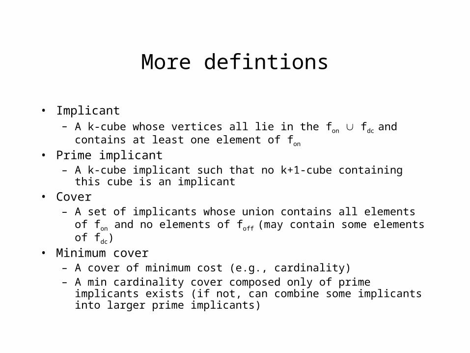
• Implicant– A k-cube whose vertices all lie in the fon fdc and contains at least one

element of fon

• Prime implicant– A k-cube implicant such that no k+1-cube containing this cube is an

implicant

• Cover– A set of implicants whose union contains all elements of fon and no

elements of foff (may contain some elements of fdc)

• Minimum cover– A cover of minimum cost (e.g., cardinality)– A min cardinality cover composed only of prime implicants exists (if not,

can combine some implicants into larger prime implicants)

Quine-McCluskey Method

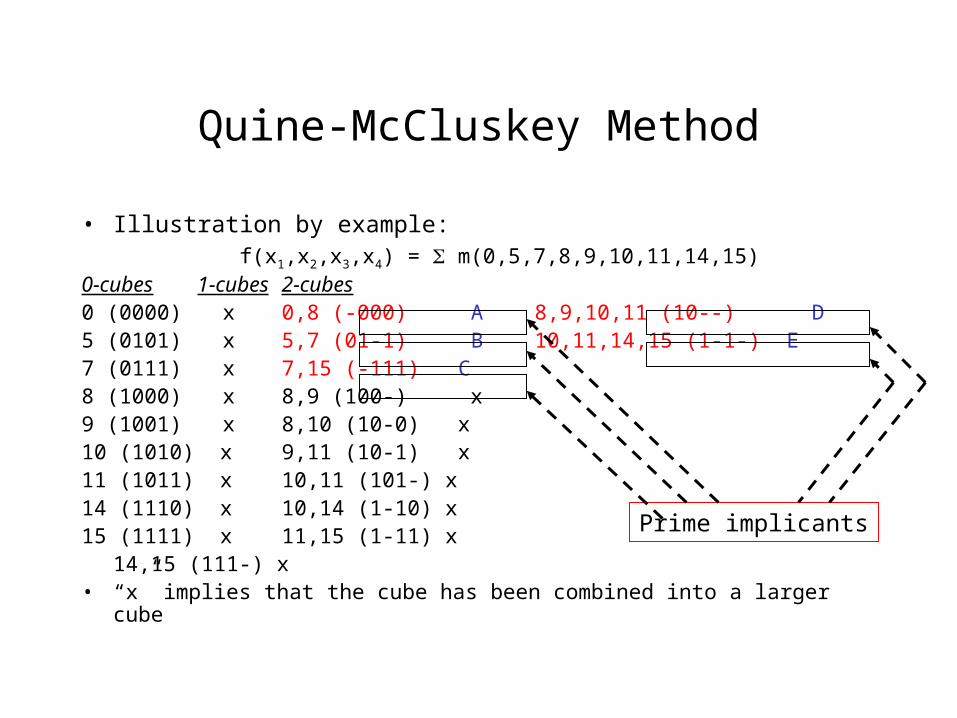
• Illustration by example:f(x1,x2,x3,x4) = m(0,5,7,8,9,10,11,14,15)

0-cubes 1-cubes 2-cubes0 (0000) x 0,8 (-000) A 8,9,10,11 (10--) D5 (0101) x 5,7 (01-1) B 10,11,14,15 (1-1-) E7 (0111) x 7,15 (-111) C8 (1000) x 8,9 (100-) x9 (1001) x 8,10 (10-0) x10 (1010) x 9,11 (10-1) x11 (1011) x 10,11 (101-) x14 (1110) x 10,14 (1-10) x15 (1111) x 11,15 (1-11) x

14,15 (111-) x• “x” implies that the cube has been combined into a larger cube

Prime implicants

Prime implicant table

• Essential Prime Implicant (PIs): – The only PI that covers a minterm (encircled in the table)– Must be included in any cover– Here, essential PIs = A,B,D,E – form a cover!– WARNING: this was luck – in general, essential PIs will not form a cover!

PI’s A

(0,8)

B

(5,7)

C

(7,15)

D

(8,9,10,11)

E

(10,11,14,15)minterms

0 x

5 x

7 x x

8 x x

9 x

10 x x

11 x x

14 x

15 x x

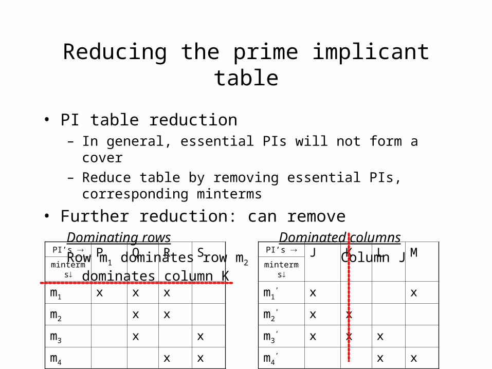
Reducing the prime implicant table

• PI table reduction– In general, essential PIs will not form a cover

– Reduce table by removing essential PIs, corresponding minterms

• Further reduction: can removeDominating rows Dominated columns

Row m1 dominates row m2 Column J dominates column K

PI’s P Q R Sminterms

m1 x x x

m2 x x

m3 x x

m4 x x

PI’s J K L Mminterms

m1’ x x

m2’ x x

m3’ x x x

m4’ x x

Branch-and-bound algorithm

• May still not have a cover– Example: example from

previous slide after removing dominating row m1 and consequently empty column P

• Can enumerate possibilities using a search tree– Binary search tree: include or

exclude PI

PI’s Q R Sminterms

m2 x x

m3 x x

m4 x x

Q

R

excludeinclude

DoneCover = {R,S}

PI’s R Sminterms

m4 x x

include excludeReduced PI table

DoneCover = {Q,S}

DoneCover = {Q,R}

Branch-and-bound algorithm (contd.)

• ESPRESSO-EXACT– Implementation of branching algorithm from previous slide

– Traversal to a leaf node of the tree yields a cover (though possibly not a minimum cost cover)

– ESPRESSO-EXACT adds bounding at any node: • If Costnode + LBsubtree > Best_cost_so_far, do not search the subtree

– Costnode = cost (e.g., number of implicants) chosen so far

– LBsubtree = a lower bound on the cost of a subtree (can be determined by solving a maximal independent set problem)

– Best_cost_so_far = cost of best cover found so far through the traversal of the search tree; initialized to

Heuristic Logic Minimization

• Apply a sequence of logic transformations to reduce a cost function

• Transformations– Expand:

• Input expansion

– Enlarge cube by combining smaller cubes

– Reduces total number of cubes

• Output expansion

– Use cube for one output to cover another

– Reduce: break up cube into sub-cubes • Increases total number of cubes

• Hope to allow overall cost reduction in a later expand operation

– Irredundant• Remove redundant cubes from a cover

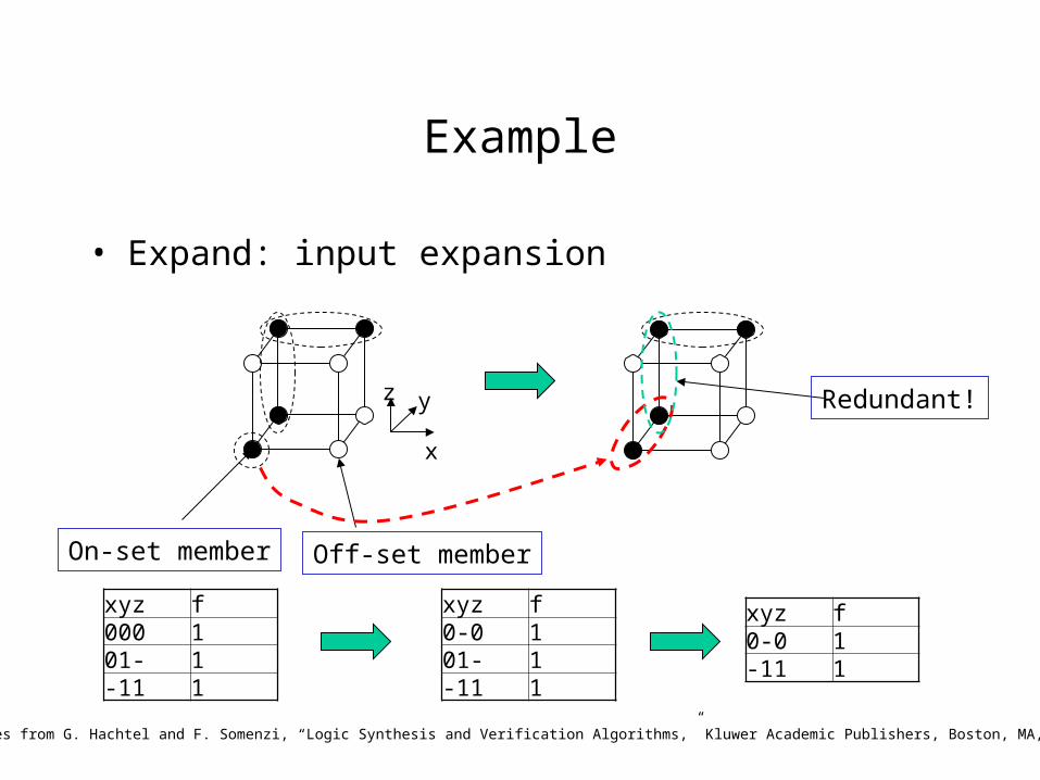
Example

• Expand: input expansion

Examples from G. Hachtel and F. Somenzi, “Logic Synthesis and Verification Algorithms,” Kluwer Academic Publishers, Boston, MA, 1996.

x

yz

Off-set memberOn-set member

xyz f000 101- 1-11 1

xyz f0-0 101- 1-11 1

xyz f0-0 1-11 1

Redundant!

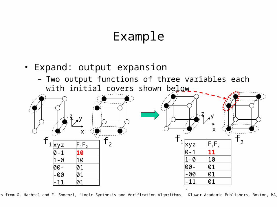
Example

• Expand: output expansion– Two output functions of three variables each with initial covers

shown below

Examples from G. Hachtel and F. Somenzi, “Logic Synthesis and Verification Algorithms,” Kluwer Academic Publishers, Boston, MA, 1996.

x

yz

f1 f2

x

yz

f1 f2xyz F1F2

0-1 101-0 1000- 01-00 01-11 01

xyz F1F2

0-1 111-0 1000- 01-00 01-11 01

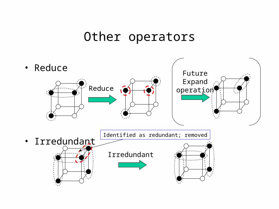
Other operators

• Reduce

• Irredundant

Reduce

FutureExpand

operation

Irredundant

Identified as redundant; removed

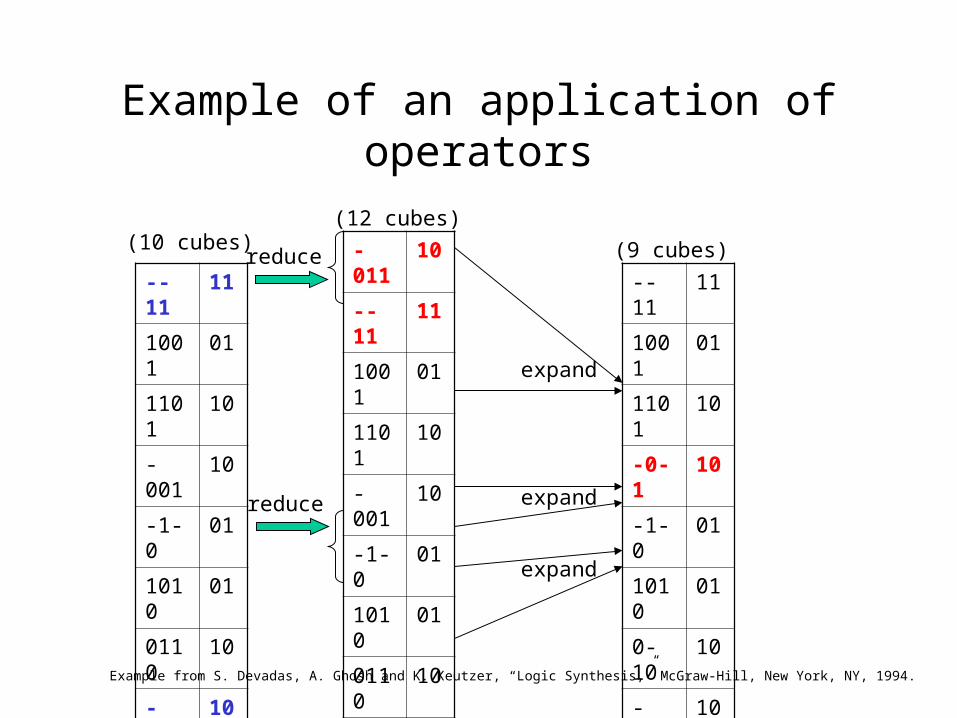
Example of an application of operators

Example from S. Devadas, A. Ghosh and K. Keutzer, “Logic Synthesis,” McGraw-Hill, New York, NY, 1994.

--11 11

1001 01

1101 10

-001 10

-1-0 01

1010 01

0110 10

-010 10

-100 10

1000 10

reduce -011 10

--11 11

1001 01

1101 10

-001 10

-1-0 01

1010 01

0110 10

0010 10

1010 10

-100 10

1000 10

reduce

--11 11

1001 01

1101 10

-0-1 10

-1-0 01

1010 01

0-10 10

-100 10

10-0 10

expand

expand

expand

(10 cubes)(12 cubes)

(9 cubes)

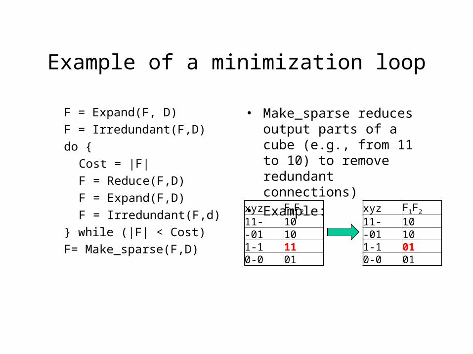
Example of a minimization loop

F = Expand(F, D)

F = Irredundant(F,D)

do {

Cost = |F|

F = Reduce(F,D)

F = Expand(F,D)

F = Irredundant(F,d)

} while (|F| < Cost)

F= Make_sparse(F,D)

• Make_sparse reduces output parts of a cube (e.g., from 11 to 10) to remove redundant connections)

• Example:

xyz F1F2

11- 10-01 101-1 110-0 01

xyz F1F2

11- 10-01 101-1 010-0 01

Implementation of operators

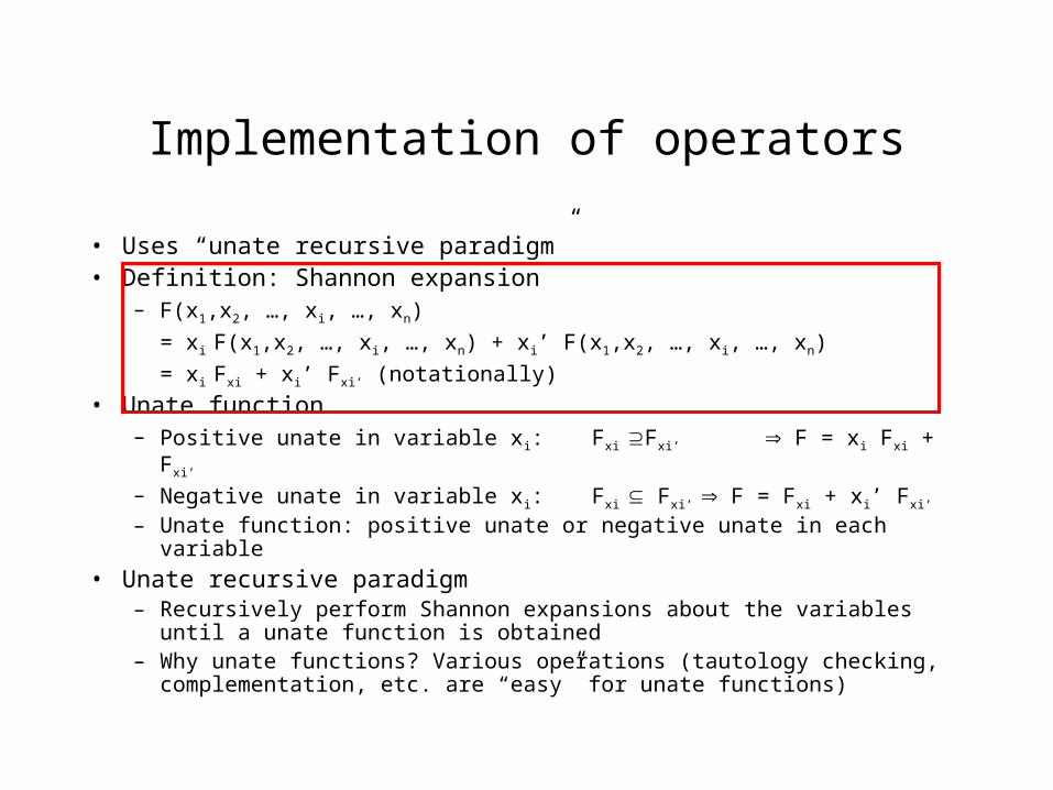
• Uses “unate recursive paradigm”• Definition: Shannon expansion

– F(x1,x2, …, xi, …, xn)

= xi F(x1,x2, …, xi, …, xn) + xi’ F(x1,x2, …, xi, …, xn)

= xi Fxi + xi’ Fxi’ (notationally)

• Unate function– Positive unate in variable xi: Fxi Fxi’ F = xi Fxi + Fxi’

– Negative unate in variable xi: Fxi Fxi’ F = Fxi + xi’ Fxi’

– Unate function: positive unate or negative unate in each variable

• Unate recursive paradigm– Recursively perform Shannon expansions about the variables until a unate

function is obtained– Why unate functions? Various operations (tautology checking,

complementation, etc. are “easy” for unate functions)

Unateness

• Example– Unate cover (not minimum)

• Every column has only 1’s and –’s, or only 0’s and –’s

– Nonunate cover: nonunate in y and z (both 1 and 0 appear in the columns)

w x y z

0 – 1 –

– – 1 –

0 – – 1

w x y z

1 – 1 –

– – 0 1

– 1 1 0

Note on notation:The table at leftrepresents the on set

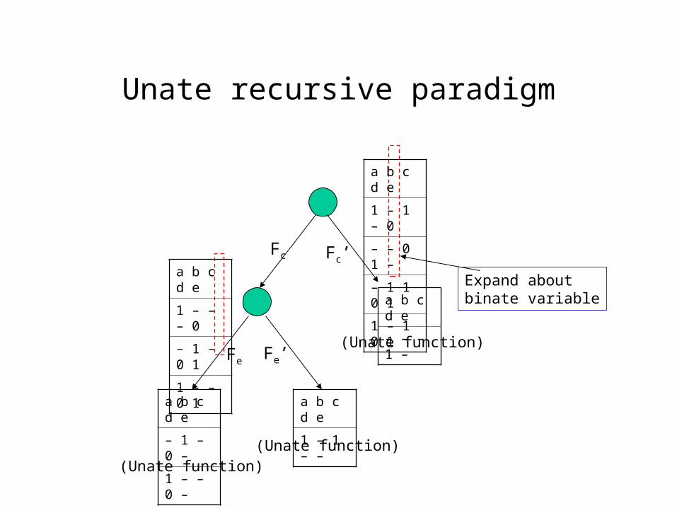
Unate recursive paradigm

a b c d e

1 – 1 – 0

– – 0 1 –

– 1 1 0 1

1 – 1 0 1

Expand aboutbinate variable

Fc Fc’

a b c d e

– – – 1 –

a b c d e

1 – – – 0

– 1 – 0 1

1 – – 0 1 (Unate function)Fe Fe’

a b c d e

– 1 – 0 –

1 – – 0 –

a b c d e

1 – 1 – –

(Unate function)(Unate function)

Example: Unate complementation

• (Example to show that unate operations are “easy”)x y z

1 0 –

1 1 0

0 – 1

x y z

– – 1

x y z

– 0 –

– 1 0

x x’

x y z

– – 0

x y z

– – –

y’y

Complement x y z

– – 1

ComplementEmpty set!

ComplementComplement

Complement

x y z

– – 0x y z

– 1 1

x y z

1 1 1

0 – 0

Basic result:

If F = x Fx + x’ Fx’ then

F’ = x (Fx)’+ x’ (Fx’)’

Proof: Let G = x (Fx)’+ x’ (Fx’)’

Show that F+G = 1 and F.G = 0

Cofactors with respect to sets of cubes

• Can generalize the Shannon expansion to

F = c Fc + c’ Fc’

where c is an set of cubes• Result: c F Fc is a

tautology• Example of finding a cofactor

with respect to a cube:– Cofactor of F =

with respect to c = [1 1 – – ]

• Fc contains elements of Fon that agree with c at all non-don’t care positions (in this example, in variables p and q)

• If so: replace non-don’t cares by “–” and copy the rest of the cube

• Following this prescription, Fc is

p q r s

1 1 0 –

0 1 – 0

1 1 1 1

p q r s

– – 0 –

– – 1 1

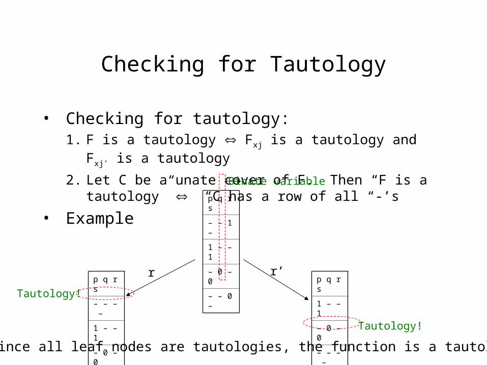
Checking for Tautology

• Checking for tautology:1. F is a tautology Fxj is a tautology and Fxj’ is a tautology

2. Let C be a unate cover of F. Then “F is a tautology” “C has a row of all “-’s

• Example p q r s

– – 1 –

1 – – 1

– 0 – 0

– – 0 –

Binate variable

r r’p q r s

– – – –

1 – – 1

– 0 – 0

p q r s

1 – – 1

– 0 – 0

– – – – Tautology!

Tautology!

Since all leaf nodes are tautologies, the function is a tautology

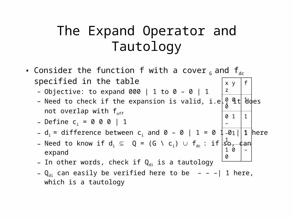
The Expand Operator and Tautology

• Consider the function f with a cover G and fdc specified in the table– Objective: to expand 000 | 1 to 0 – 0 | 1

– Need to check if the expansion is valid, i.e., it does

not overlap with foff

– Define ci = 0 0 0 | 1

– di = difference between ci and 0 – 0 | 1 = 0 1 0 | 1 here

– Need to know if di Q = (G \ ci) fdc : if so, can expand

– In other words, check if Qdi is a tautology

– Qdi can easily be verified here to be – – –| 1 here, which is a tautology

x y z f

0 0 0 1

0 1 – 1

– 1 1 1

1 0 0 –

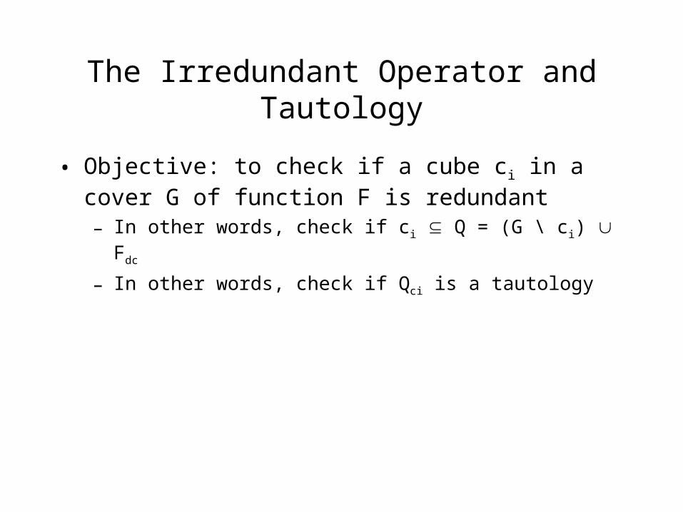
The Irredundant Operator and Tautology

• Objective: to check if a cube ci in a cover G of function F is redundant– In other words, check if ci Q = (G \ ci) Fdc

– In other words, check if Qci is a tautology

Multilevel logic optimization

• Motivation– Two-level optimization (SOP, POS) is too limiting

– Useful for structures like PLA’s, but most circuits are not designed in that way

– May require gates with a large number of inputs

– Restricts “sharing” of logic gates between outputs

– Multilevel optimization permits more than two levels of gates between the inputs and the outputs

– Necessarily heuristic

Reference for this part: G. De Micheli, “Synthesis and Optimization of Digital Circuits,” McGraw-Hill, New York, NY, 1994.

Basic Transformations

• Eliminationr = p + a’; s = r + b’ s = p + a’ + b’

• Decompositionv = a’d + bd + cd + a’e j = a’ + b + c; v = j d + a’e

• Extractionp = ce+de; t = ac+ad+bc+bd+e k = c+d; p = ke; t = ka+kb+e

• Simplificationu = q’c+qc’+qc u = q+c

• Substitutiont = ka+kb+e; q = a+b t = kq+e

• (Others exist; these are the most common)

Transformations

• Apply the transformations heuristically

• Two methods:– Algorithmic: algorithm for each transformation type

– Rule-based: according to a set of rules injected into the system by a human designer

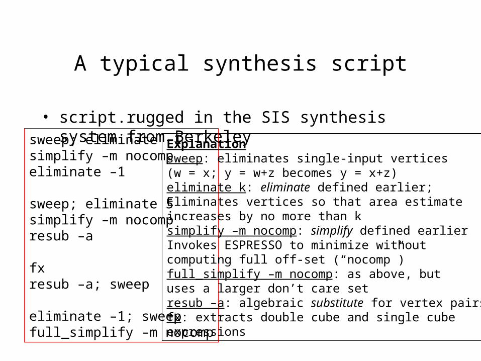
A typical synthesis script

• script.rugged in the SIS synthesis system from Berkeleysweep; eliminate –1simplify –m nocompeliminate –1

sweep; eliminate 5simplify –m nocompresub –a

fxresub –a; sweep

eliminate –1; sweepfull_simplify –m nocomp

Explanationsweep: eliminates single-input vertices(w = x; y = w+z becomes y = x+z)eliminate k: eliminate defined earlier;Eliminates vertices so that area estimateincreases by no more than k simplify –m nocomp: simplify defined earlierInvokes ESPRESSO to minimize withoutcomputing full off-set (“nocomp”)full_simplify –m nocomp: as above, butuses a larger don’t care setresub –a: algebraic substitute for vertex pairsfx: extracts double cube and single cubeexpressions

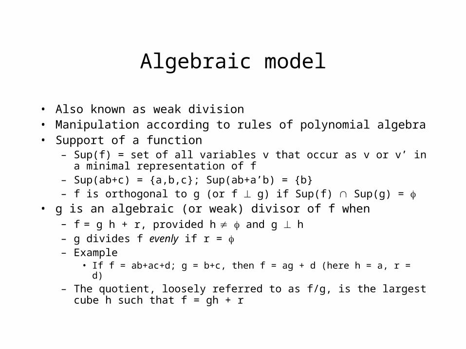
Algebraic model

• Also known as weak division• Manipulation according to rules of polynomial algebra• Support of a function

– Sup(f) = set of all variables v that occur as v or v’ in a minimal representation of f

– Sup(ab+c) = {a,b,c}; Sup(ab+a’b) = {b}– f is orthogonal to g (or f g) if Sup(f) Sup(g) =

• g is an algebraic (or weak) divisor of f when– f = g h + r, provided h and g h– g divides f evenly if r = – Example

• If f = ab+ac+d; g = b+c, then f = ag + d (here h = a, r = d)

– The quotient, loosely referred to as f/g, is the largest cube h such that f = gh + r

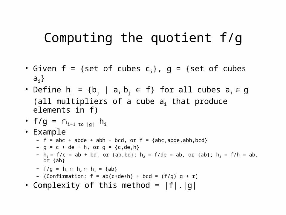
Computing the quotient f/g

• Given f = {set of cubes ci}, g = {set of cubes ai}• Define hi = {bj | ai bj f} for all cubes ai g

(all multipliers of a cube ai that produce elements in f)• f/g = i=1 to |g| hi

• Example– f = abc + abde + abh + bcd, or f = {abc,abde,abh,bcd}– g = c + de + h, or g = {c,de,h}– h1 = f/c = ab + bd, or {ab,bd}; h2 = f/de = ab, or {ab}; h3 = f/h = ab, or {ab}

– f/g = h1 h2 h3 = {ab}– (Confirmation: f = ab(c+de+h) + bcd = (f/g) g + r)

• Complexity of this method = |f|.|g|

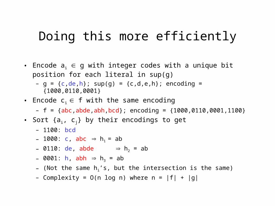
Doing this more efficiently

• Encode ai g with integer codes with a unique bit position for each literal in sup(g)

– g = {c,de,h}; sup(g) = {c,d,e,h}; encoding = {1000,0110,0001}

• Encode ci f with the same encoding

– f = {abc,abde,abh,bcd}; encoding = {1000,0110,0001,1100}

• Sort {ai, cj} by their encodings to get

– 1100: bcd

– 1000: c, abc h1 = ab

– 0110: de, abde h2 = ab

– 0001: h, abh h3 = ab

– (Not the same hi’s, but the intersection is the same)

– Complexity = O(n log n) where n = |f| + |g|

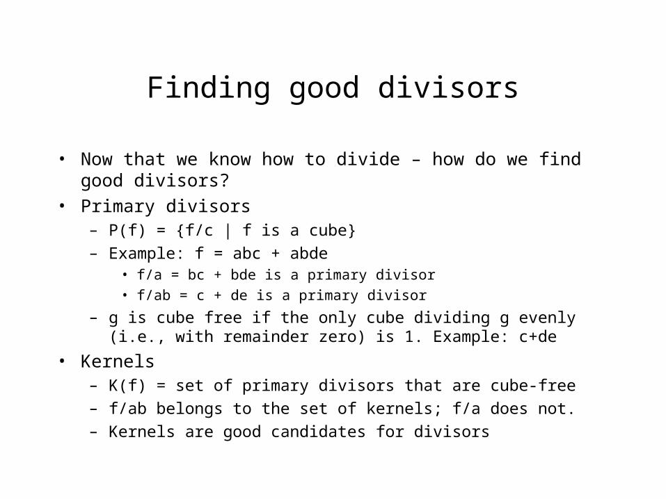
Finding good divisors

• Now that we know how to divide – how do we find good divisors?

• Primary divisors– P(f) = {f/c | f is a cube}

– Example: f = abc + abde• f/a = bc + bde is a primary divisor

• f/ab = c + de is a primary divisor

– g is cube free if the only cube dividing g evenly (i.e., with remainder zero) is 1. Example: c+de

• Kernels– K(f) = set of primary divisors that are cube-free

– f/ab belongs to the set of kernels; f/a does not.

– Kernels are good candidates for divisors

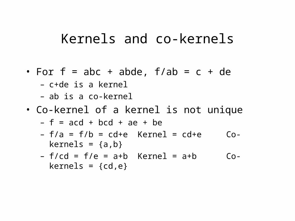
Kernels and co-kernels

• For f = abc + abde, f/ab = c + de– c+de is a kernel

– ab is a co-kernel

• Co-kernel of a kernel is not unique– f = acd + bcd + ae + be

– f/a = f/b = cd+e Kernel = cd+e Co-kernels = {a,b}

– f/cd = f/e = a+b Kernel = a+b Co-kernels = {cd,e}

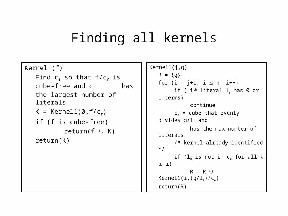
Finding all kernels

Kernel (f)

Find cf so that f/cf is cube-free and cf has the largest number of

literals

K = Kernel1(0,f/cf)

if (f is cube-free)

return(f K)

return(K)

Kernel1(j,g)

R = {g}

for (i = j+1; i n; i++)

if ( ith literal li has 0 or 1 terms)

continue

ce = cube that evenly divides g/li and

has the max number of literals

/* kernel already identified */

if (lk is not in ce for all k i)

R = R Kernel1(i,(g/li)/ce)

return(R)

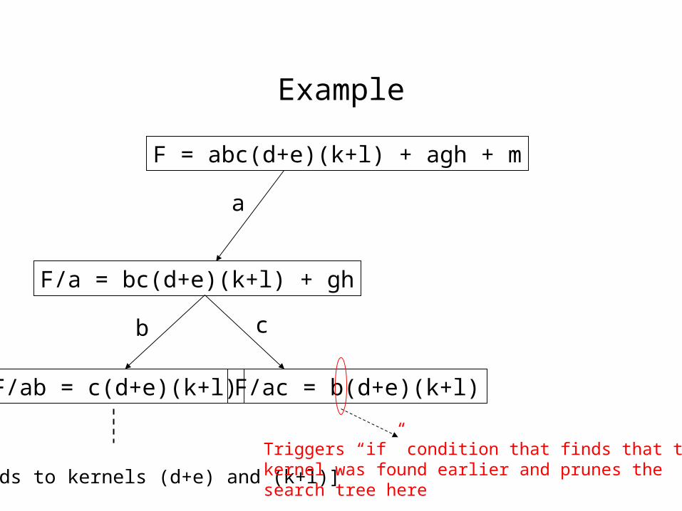
Example

F = abc(d+e)(k+l) + agh + m

F/a = bc(d+e)(k+l) + gh

a

b c

F/ab = c(d+e)(k+l)

[Leads to kernels (d+e) and (k+l)]

F/ac = b(d+e)(k+l)

Triggers “if” condition that finds that thiskernel was found earlier and prunes the search tree here

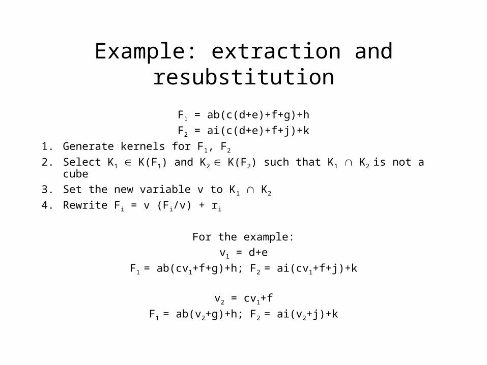
Example: extraction and resubstitution

F1 = ab(c(d+e)+f+g)+h

F2 = ai(c(d+e)+f+j)+k

1. Generate kernels for F1, F2

2. Select K1 K(F1) and K2 K(F2) such that K1 K2 is not a cube

3. Set the new variable v to K1 K2

4. Rewrite Fi = v (Fi/v) + ri

For the example:

v1 = d+e

F1 = ab(cv1+f+g)+h; F2 = ai(cv1+f+j)+k

v2 = cv1+f

F1 = ab(v2+g)+h; F2 = ai(v2+j)+k

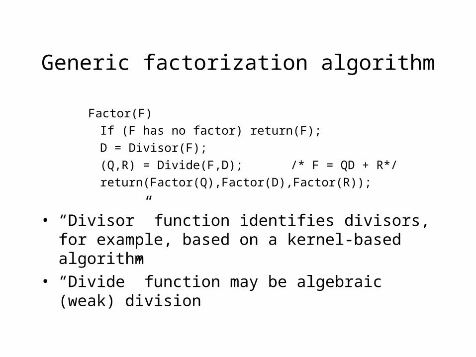
Generic factorization algorithm

Factor(F)

If (F has no factor) return(F);

D = Divisor(F);

(Q,R) = Divide(F,D); /* F = QD + R*/

return(Factor(Q),Factor(D),Factor(R));

• “Divisor” function identifies divisors, for example, based on a kernel-based algorithm

• “Divide” function may be algebraic (weak) division

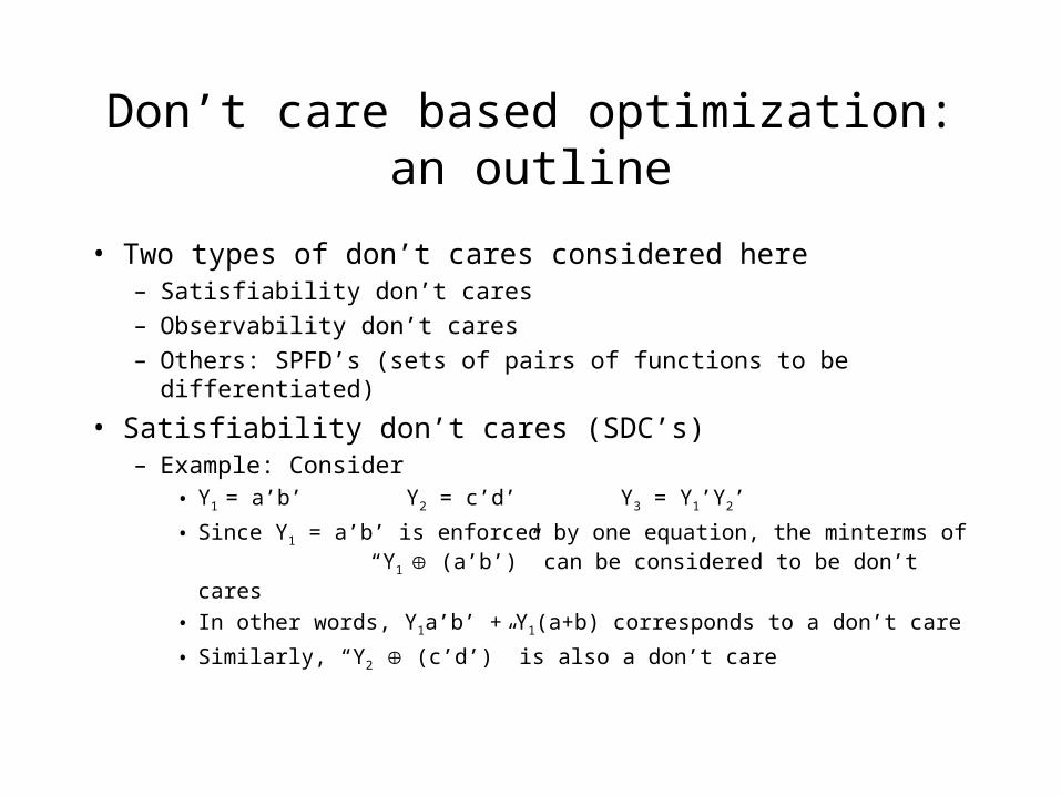
Don’t care based optimization: an outline

• Two types of don’t cares considered here– Satisfiability don’t cares

– Observability don’t cares

– Others: SPFD’s (sets of pairs of functions to be differentiated)

• Satisfiability don’t cares (SDC’s)– Example: Consider

• Y1 = a’b’ Y2 = c’d’ Y3 = Y1’Y2’

• Since Y1 = a’b’ is enforced by one equation, the minterms of “Y1 (a’b’)” can be considered to be don’t cares

• In other words, Y1a’b’ + Y1(a+b) corresponds to a don’t care

• Similarly, “Y2 (c’d’)” is also a don’t care

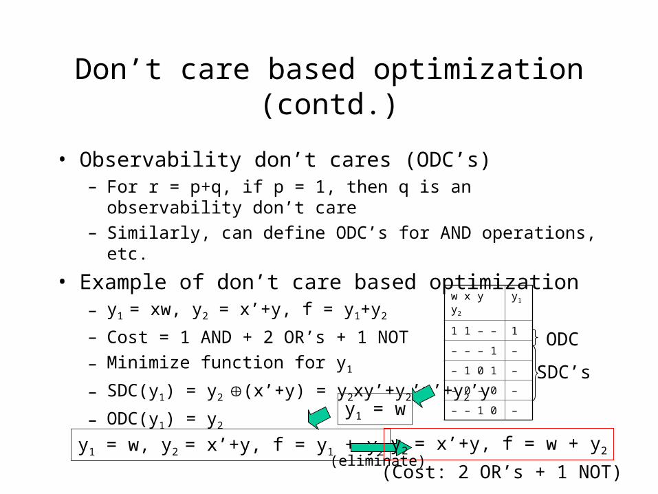
Don’t care based optimization (contd.)

• Observability don’t cares (ODC’s)– For r = p+q, if p = 1, then q is an observability don’t care

– Similarly, can define ODC’s for AND operations, etc.

• Example of don’t care based optimization– y1 = xw, y2 = x’+y, f = y1+y2

– Cost = 1 AND + 2 OR’s + 1 NOT

– Minimize function for y1

– SDC(y1) = y2 (x’+y) = y2xy’+y2’x’+y2’y

– ODC(y1) = y2

w x y y2 y1

1 1 – – 1

– – – 1 –

– 1 0 1 –

– 0 – 0 –

– – 1 0 –y1 = w

ODC

SDC’s

y1 = w, y2 = x’+y, f = y1 + y2 y2 = x’+y, f = w + y2(eliminate)

(Cost: 2 OR’s + 1 NOT)

Acknowledgements

• Hardly anything in these notes is original, and they borrow heavily from sources such as– G. De Micheli, “Synthesis and Optimization of Digital Circuits,”

McGraw-Hill, New York, NY, 1994.– S. Devadas, A. Ghosh and K. Keutzer, “Logic Synthesis,” McGraw-Hill,

New York, NY, 1994– G. Hachtel and F. Somenzi, “Logic Synthesis and Verification

Algorithms,” Kluwer Academic Publishers, Boston, MA, 1996.– Notes from Prof. Brayton's synthesis class at UC Berkeley (http://www-

cad.eecs.berkeley.edu/~brayton/courses/219b/219b.html)– Notes from Prof. Devadas's CAD class at MIT

(http://glenfiddich.lcs.mit.edu/~devadas/6.373/lectures)– Possibly other sources that I may have omitted to acknowledge (my

apologies)