Logistic Regression ILogistic Regression I

HRP 261 2/09/04HRP 261 2/09/04

Related reading: Related reading: chapters 4.1-4.2 and 5.1-5.5 ofchapters 4.1-4.2 and 5.1-5.5 of Agresti Agresti

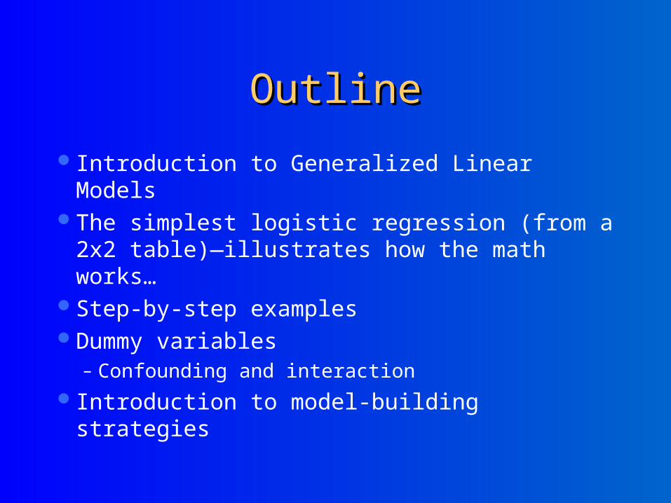
OutlineOutline

Introduction to Generalized Linear ModelsThe simplest logistic regression (from a 2x2

table)—illustrates how the math works…Step-by-step examples Dummy variables

– Confounding and interaction

Introduction to model-building strategies

GeneralGeneralized ized Linear ModelsLinear Models(chapter 4 of (chapter 4 of AgrestiAgresti))

Twice the generality!The generalized linear model is a

generalization of the general linear model

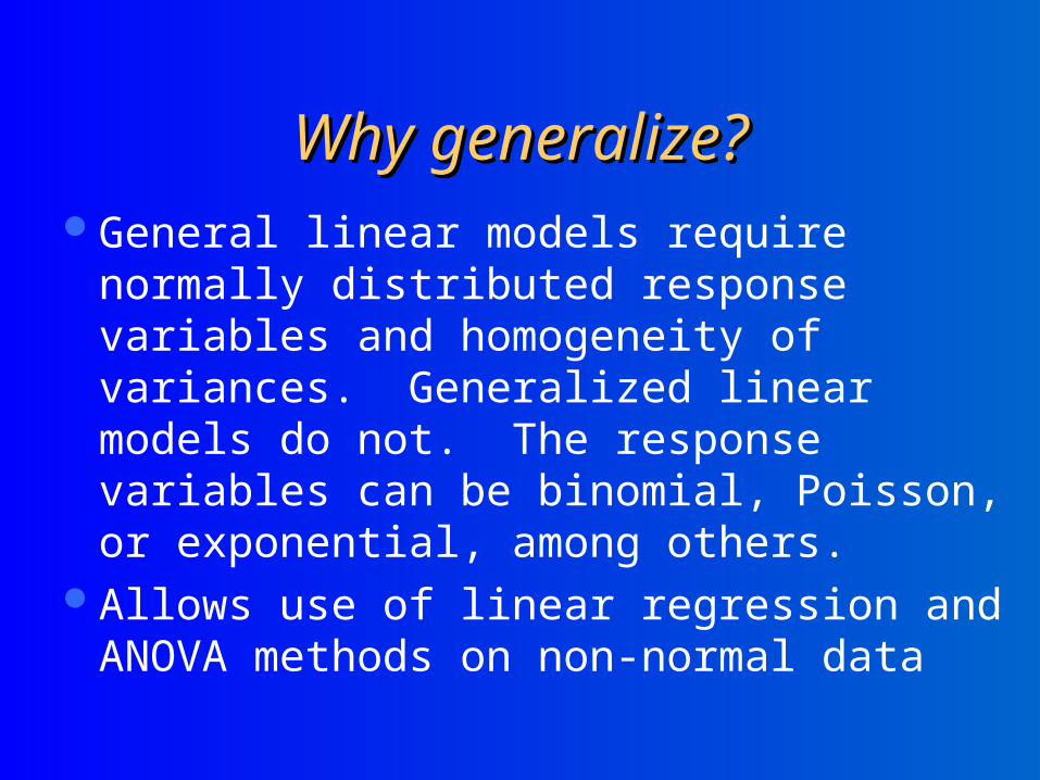
Why generalize?Why generalize?General linear models require normally

distributed response variables and homogeneity of variances. Generalized linear models do not. The response variables can be binomial, Poisson, or exponential, among others.

Allows use of linear regression and ANOVA methods on non-normal data

Why not just transform?Why not just transform?

A traditional way of analyzing non-normal data is to transform the response variable so it is approximately normal, with constant variance. And then apply least squares regression.

E.g.,derivative[(lnYi-(mx+b))2]=0

But then g(Yi) has to be normal, with constant variance.

“Maximum likelihood” is more general than least squares

Example : The Bernouilli (binomial) Example : The Bernouilli (binomial) distributiondistribution

Smoking (cigarettes/day)

Lung cancer; yes/no

y

n

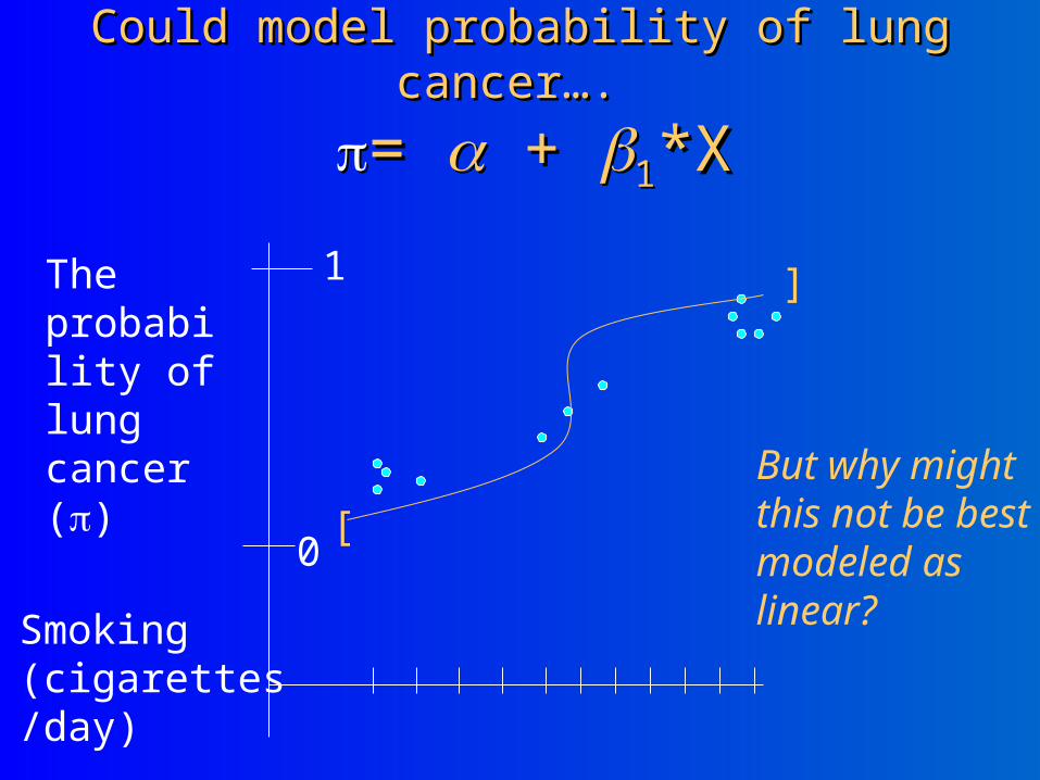
Could model probability of lung Could model probability of lung cancer…. cancer….

= = + + 11*X*X

Smoking (cigarettes/day)

The probability of lung cancer ()

1

0

But why might this not be best modeled as linear?

[

]

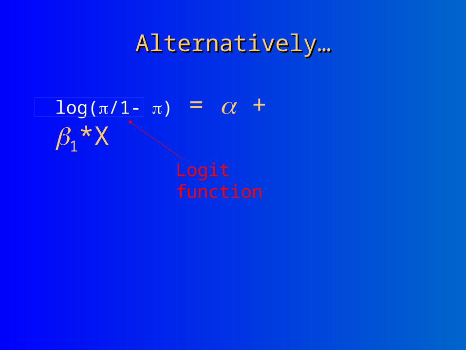
Alternatively…Alternatively…

log(/1- ) = + 1*X

Logit function

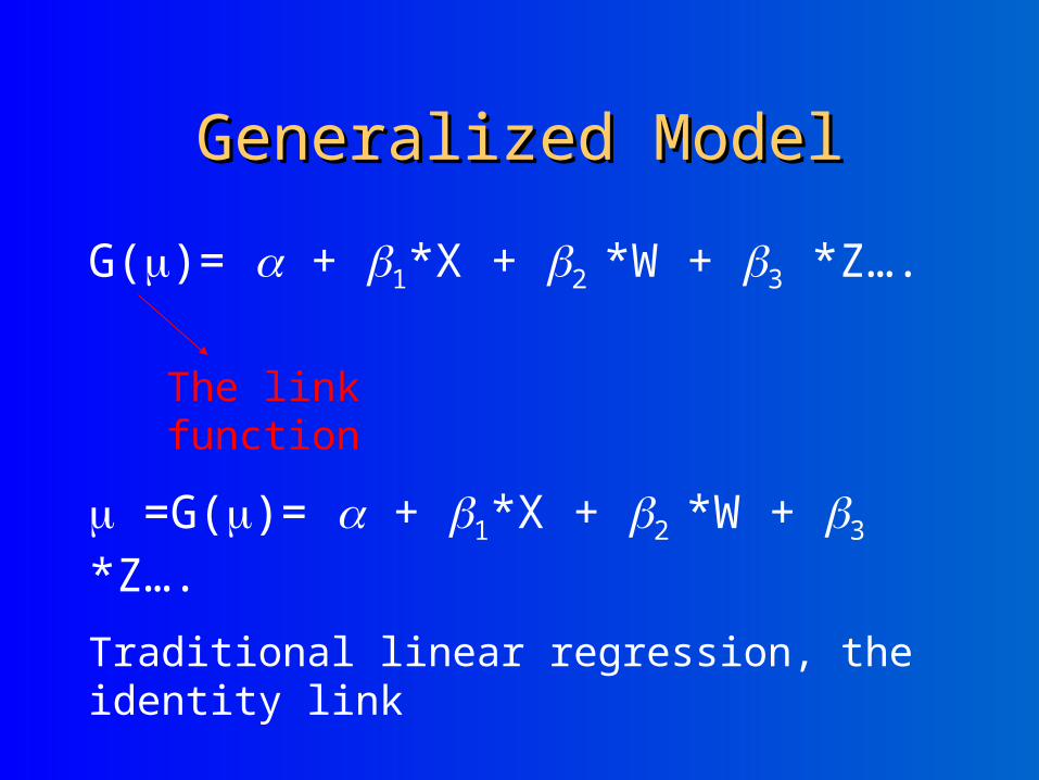
Generalized ModelGeneralized Model

G()= + 1*X + 2 *W + 3 *Z….

The link function

=G()= + 1*X + 2 *W + 3 *Z….

Traditional linear regression, the identity link

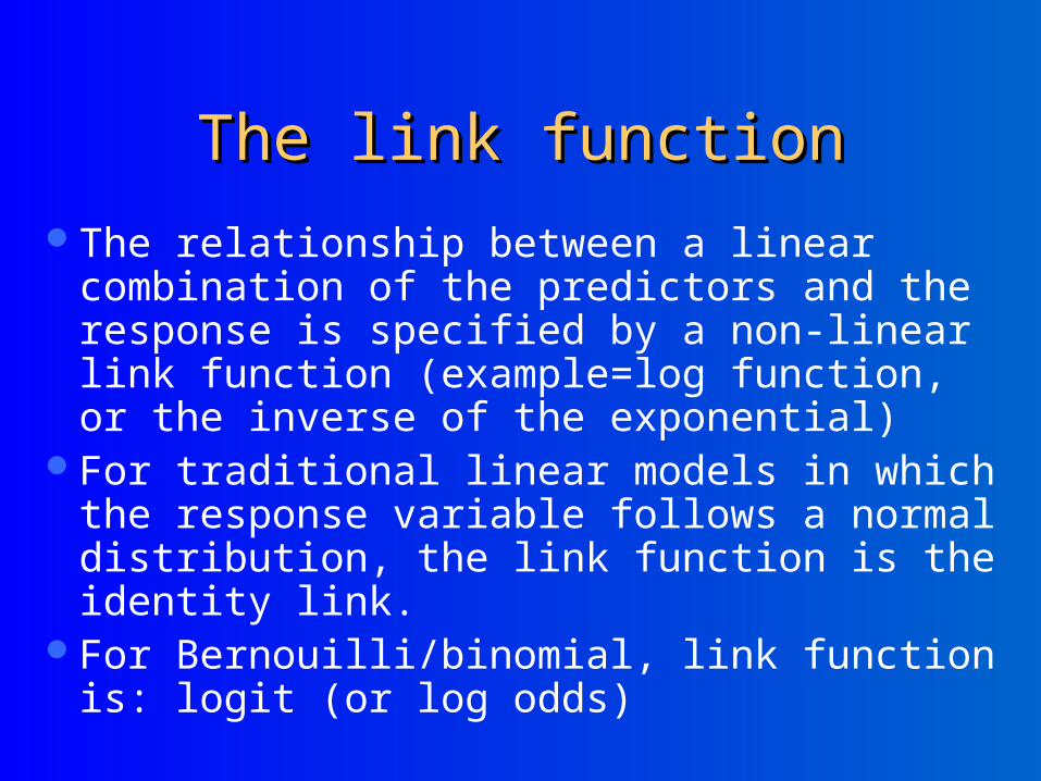
The link functionThe link function

The relationship between a linear combination of the predictors and the response is specified by a non-linear link function (example=log function, or the inverse of the exponential)

For traditional linear models in which the response variable follows a normal distribution, the link function is the identity link.

For Bernouilli/binomial, link function is: logit (or log odds)

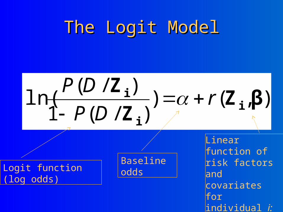
The Logit ModelThe Logit Model

),())/(1

)/(ln( βZ

Z

Zi

i

i rDP

DP

Logit function (log odds)Baseline odds

Linear function of risk factors and covariates for individual i:

1x1 + 2x2 + 3x3 + 4x4

…

Relating odds to probabilitiesRelating odds to probabilities

)(

)(

),(

1)/(

)/(1

)/(

),()()/()/(

),()/(

),()/(

onmanipulati algebraic

βZ

βZ

i

βZ

i

i

i

i

βiZβiZ

iZ

iZ

βiZ

iZ

βiZ

iZ

i

Z

Z

Z

,r

,r

r

e

eDP

eDP

DP

re

,reDPDP

reDP

reDP

odds

algebra

probability

),(),(

),(

),(

),(

1

1

11)/(~

1)/(

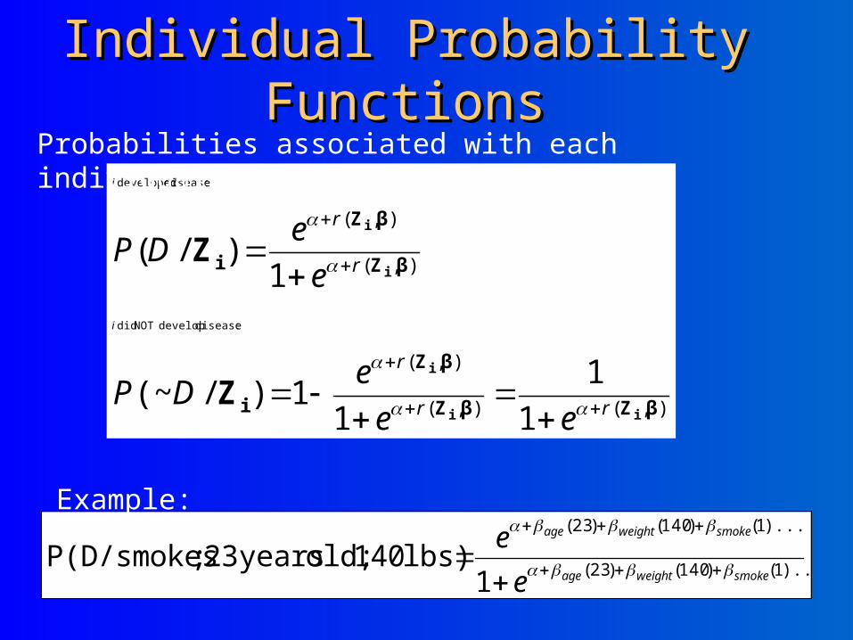
:disease develop NOT did

:disease developed

βZβZ

βZ

i

βZ

βZ

i

ii

i

i

i

Z

Z

rr

r

r

r

ee

eDP

e

eDP

i

i

Probabilities associated with each individual’s outcome:

)...1()140()23(

)...1()140()23(

1 lbs) 140 old; years 23 ;P(D/smokes

smokeweightage

smokeweightage

e

e

Individual Probability FunctionsIndividual Probability Functions

Example:

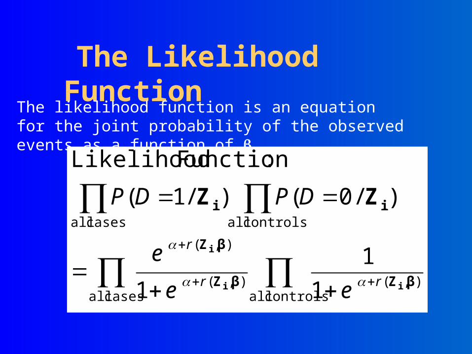
controls all),(

cases all),(

),(

controls allcases all

1

1

1

)/0()/1(

:Function Likelihood

βZβZ

βZ

ii

ii

i

ZZ

rr

r

ee

e

DPDP

The Likelihood Function

The likelihood function is an equation for the joint probability of the observed events as a function of

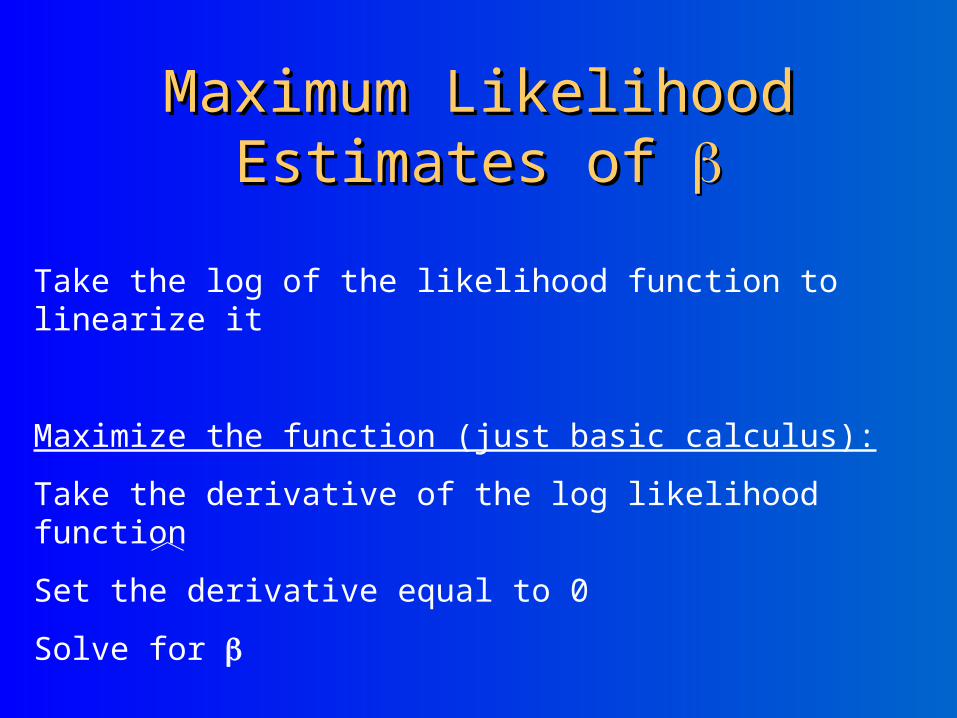
Maximum Likelihood Maximum Likelihood Estimates of Estimates of

Take the log of the likelihood function to linearize it

Maximize the function (just basic calculus):

Take the derivative of the log likelihood function

Set the derivative equal to 0

Solve for

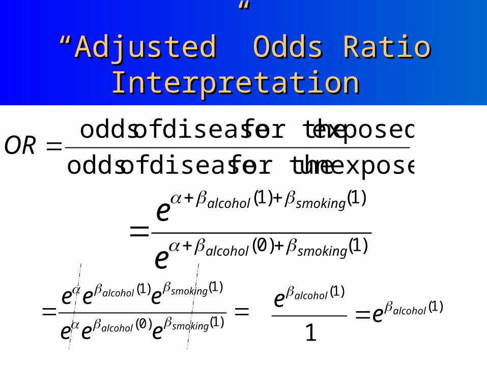
““Adjusted” Odds Ratio Adjusted” Odds Ratio Interpretation Interpretation

unexposed for the disease of odds

exposed for the disease of oddsOR

)1()0(

)1()1(

smokingalcohol

smokingalcohol

e

e

)1()0(

)1()1(

smokingalcohol

smokingalcohol

eee

eee

)1(

)1(

1alcohol

alcohol

ee

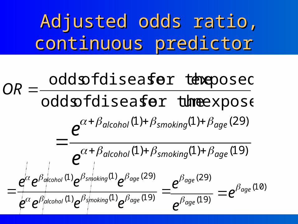
Adjusted odds ratio, Adjusted odds ratio, continuous predictor continuous predictor

unexposed for the disease of odds

exposed for the disease of oddsOR

)19()1()1(

)29()1()1(

agesmokingalcohol

agesmokingalcohol

e

e

)19()1()1(

)29()1()1(

agesmokingalcohol

agesmokingalcohol

eeee

eeee

)10(

)19(

)29(age

age

age

ee

e

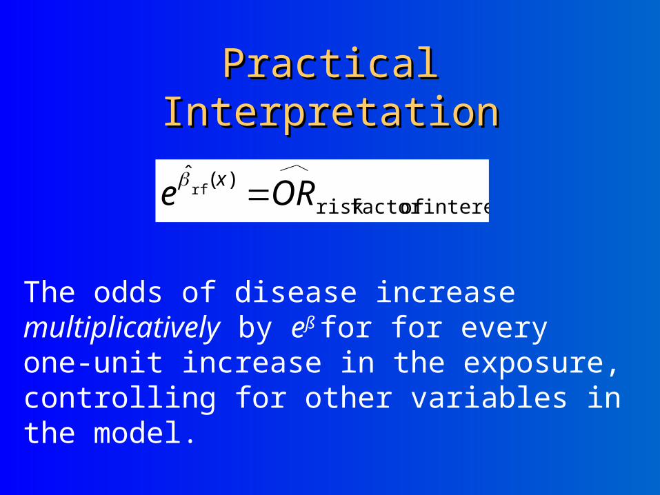
Practical InterpretationPractical Interpretation

interest offactor risk

)(ˆrf ORe

x

The odds of disease increase multiplicatively by eß

for for every one-unit increase in the exposure, controlling for other variables in the model.

Simple Logistic RegressionSimple Logistic Regression

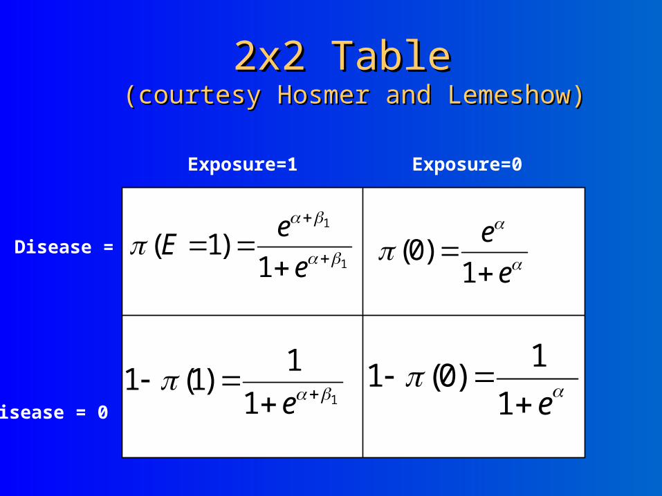
2x2 Table 2x2 Table (courtesy Hosmer and Lemeshow)(courtesy Hosmer and Lemeshow)

 

Exposure=1 Exposure=0

 Disease = 1

Disease = 0 

1

1

1)1(

e

eE

e

e

1)0(

11

1)1(1

e e

1

1)0(1

e

ee

e

ee

OR

11

1

11

1

1

1

1

1

(courtesy Hosmer and Lemeshow)(courtesy Hosmer and Lemeshow)

Odds Ratio for simple 2x2 Table Odds Ratio for simple 2x2 Table

e

e 111 )( ee

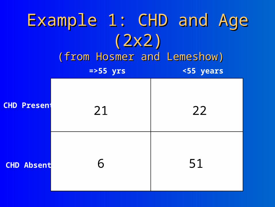
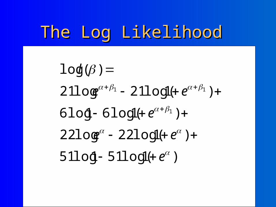
Example 1: CHD and Age Example 1: CHD and Age (2x2)(2x2)

(from Hosmer and Lemeshow) (from Hosmer and Lemeshow)

 

=>55 yrs <55 years

 CHD Present

CHD Absent 

21 22

6 51

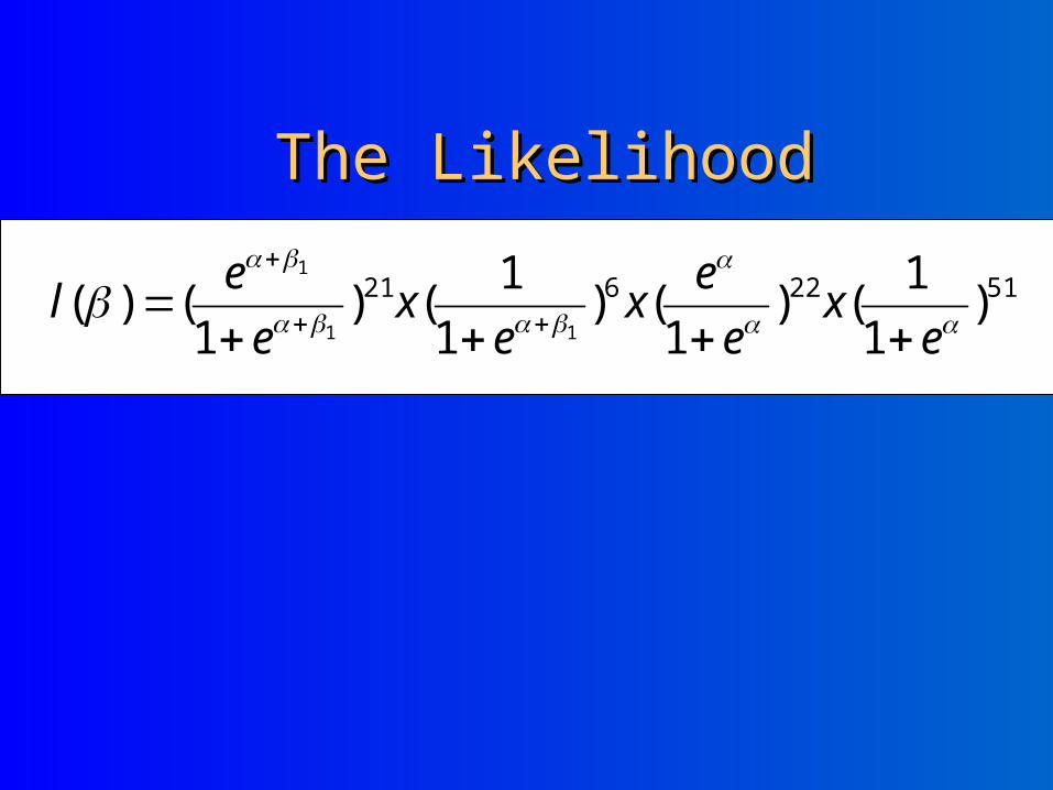
5122621 )1

1()

1()

1

1()

1()(

11

1

e

xe

ex

ex

e

el

The LikelihoodThe Likelihood

)1log(511log51

)1log(22log22

)1log(61log6

)1log(21log21

)(log

1

11

e

ee

e

ee

l

The Log LikelihoodThe Log Likelihood

The Log Likelihood, cont.The Log Likelihood, cont.

)1log(510

)1log(2222

)1log(60

)1log(21)(21

)(log

loglogloglog

1

1

111

1

1

e

e

e

e

l

eeeee

recall

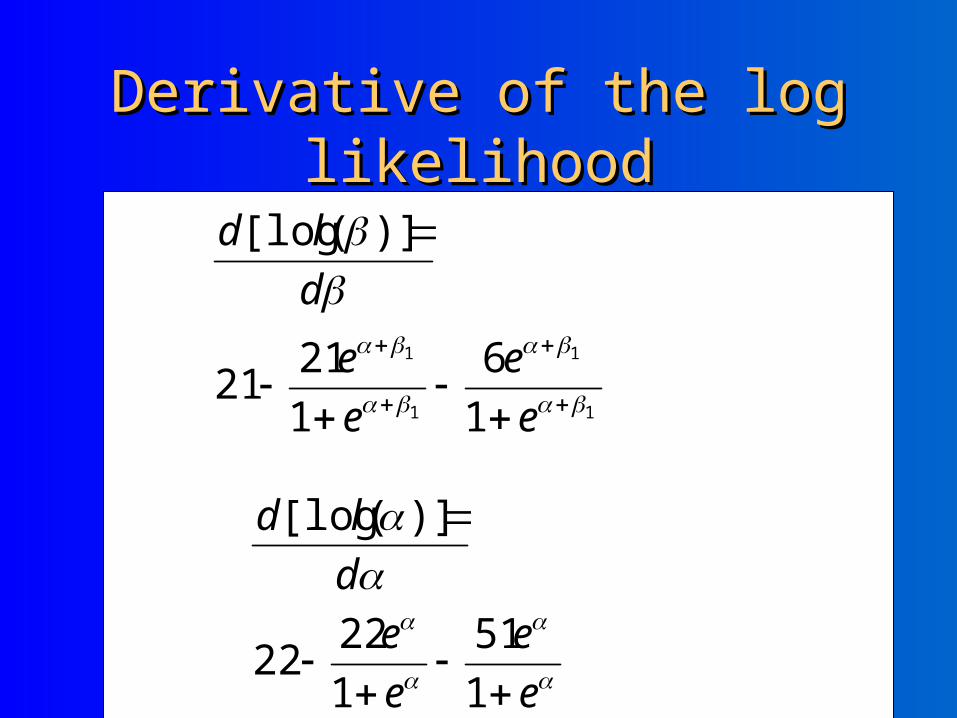
Derivative of the log likelihoodDerivative of the log likelihood

1

1

1

1

1

6

1

2121

)]([log

e

e

e

e

d

ld

e

e

e

e

d

ld

1

51

1

2222

)]([log

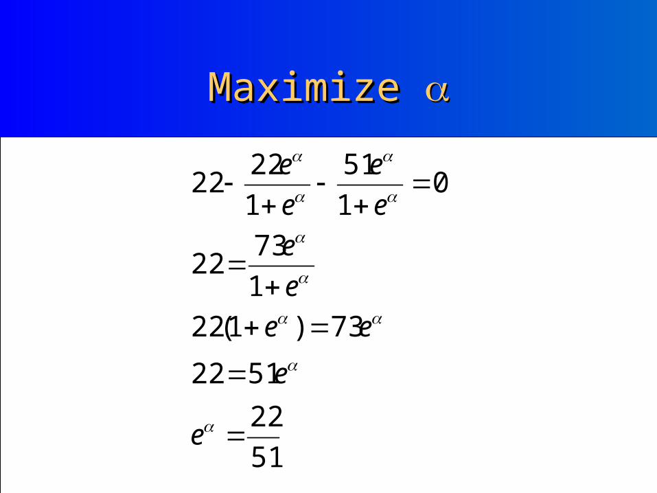
Maximize Maximize

51

22

5122

73)1(22

1

7322

01

51

1

2222

e

e

ee

e

e

e

e

e

e

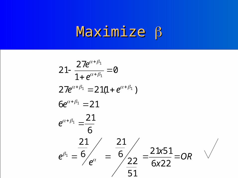
Maximize Maximize

ORx

xe

e

e

e

ee

e

e

226

5121

5122

621

621

6

21

216

)1(2127

01

2721

1

1

1

11

1

1

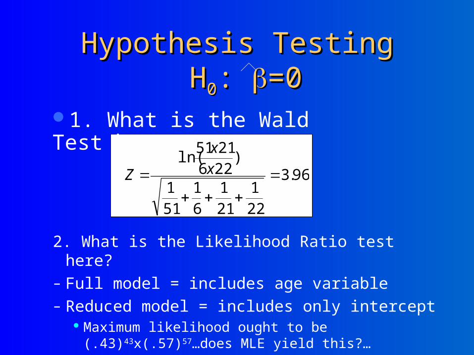
Hypothesis TestingHypothesis Testing H H00: : =0=0

2. The Likelihood Ratio test:

1. The Wald test:

)ˆ(error standard asymptotic

0ˆ

Z

2~))](ln(2[))(ln(2

)(

)(ln2

pfullLreducedL

fullL

reducedL

Reduced=reduced model with k parameters; Full=full model with k+p parameters

3. The Score Test (deferred for later discussion)

Hypothesis TestingHypothesis Testing H H00: : =0=0

2. What is the Likelihood Ratio test here?– Full model = includes age variable– Reduced model = includes only intercept

Maximum likelihood ought to be (.43)43x(.57)57…does MLE yield this?…

96.3

221

211

61

511

)2262151

ln(

x

x

Z

1. What is the Wald Test here?

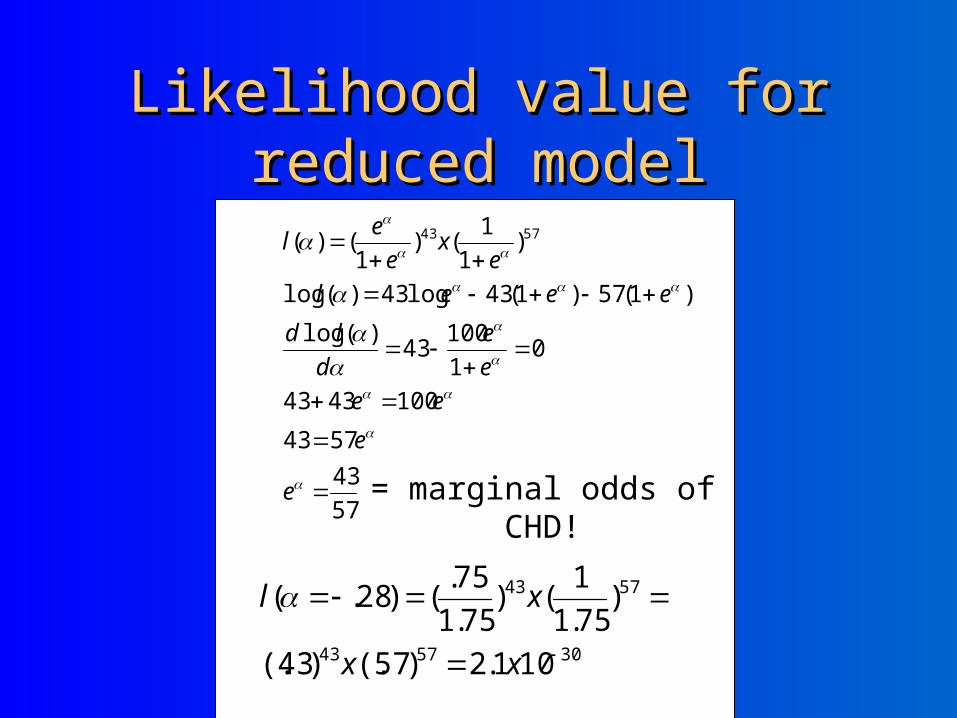
Likelihood value for reduced Likelihood value for reduced modelmodel

57

43

5743

1004343

01

10043

)(log

)1(57)1(43log43)(log

)1

1()

1()( 5743

e

e

ee

e

e

d

ld

eeel

ex

e

el

= marginal odds of CHD!

305743

5743

101.2)57(.)43(.

)75.1

1()

75.1

75.()28.(

xx

xl

Likelihood value of full modelLikelihood value of full model

265122621

5122621

1043.2)43.1

1()

43.1

43.()

5.4

1()

5.4

5.3(

)

5122

1

1()

5122

1

5122

()

621

1

1()

621

1

621

()(

xxxx

xxxl

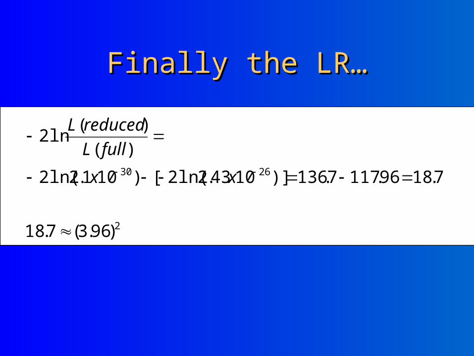
Finally the LR…Finally the LR…

2

2630

)96.3(7.18

7.1896.1177.136)]1043.2ln(2[)101.2ln(2

)(

)(ln2

xx

fullL

reducedL

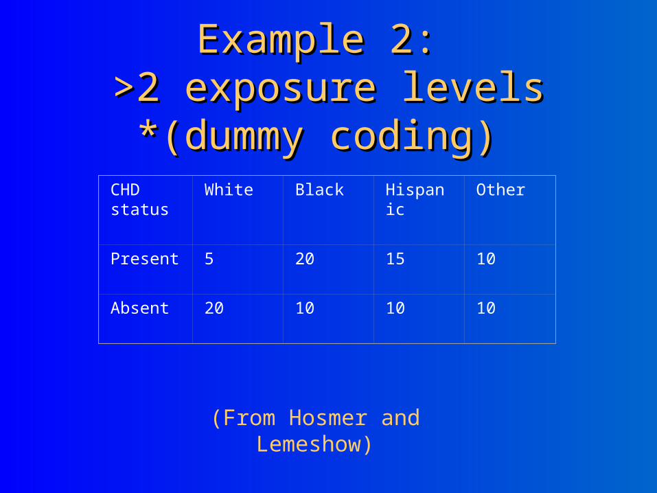
Example 2: Example 2: >2 exposure levels>2 exposure levels*(dummy coding) *(dummy coding)

CHD status

White Black Hispanic Other

Present 5 20 15 10

Absent 20 10 10 10

(From Hosmer and Lemeshow)

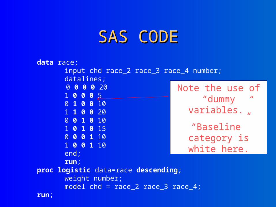
SAS CODESAS CODEdata race;

input chd race_2 race_3 race_4 number;datalines;

0 0 0 0 201 0 0 0 50 1 0 0 101 1 0 0 200 0 1 0 101 0 1 0 150 0 0 1 101 0 0 1 10end;run;

proc logistic data=race descending;weight number;model chd = race_2 race_3 race_4;

run;

Note the use of “dummy variables.”

“Baseline” category is white here.

What’s the likelihood here?What’s the likelihood here?

10101015

1020205

)1

1()

1()

1

1()

1( x

)1

1()

1()

1

1()

1()(

otherwhiteotherwhite

otherwhite

hispwhitehispwhite

hispwhite

blackwhiteblackwhite

blackwhite

whitewhite

white

ex

e

e

ex

e

e

ex

e

ex

ex

e

el

β

SAS OUTPUT – model fitSAS OUTPUT – model fit 

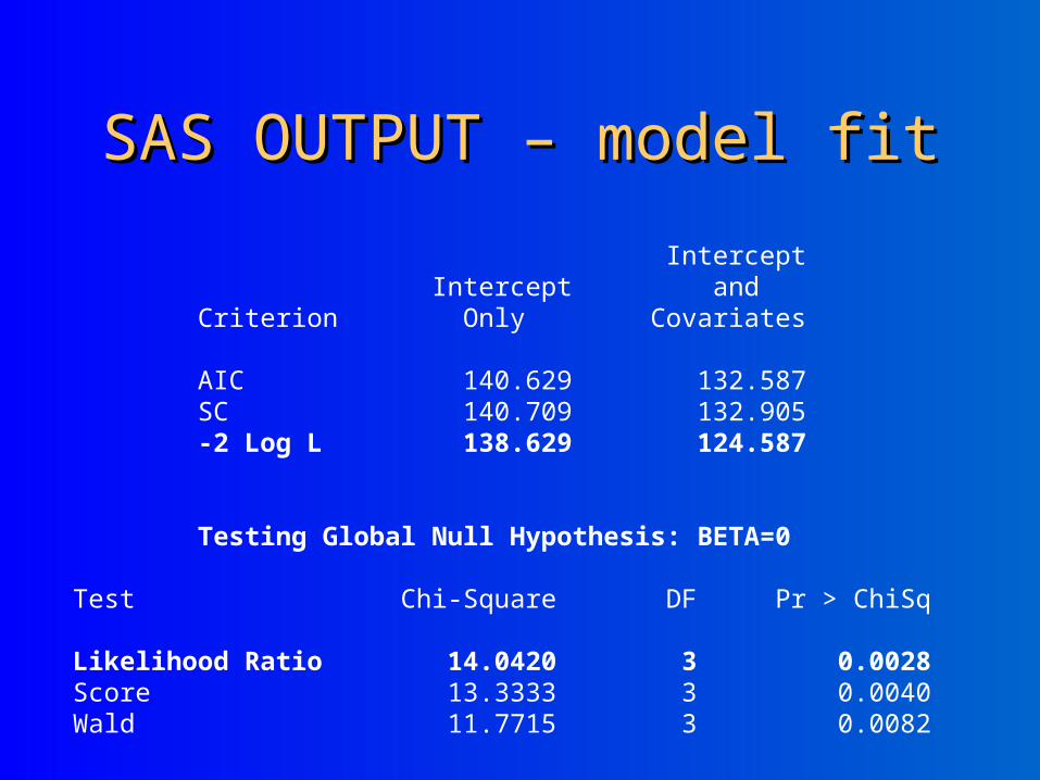
Intercept Intercept and Criterion Only Covariates  AIC 140.629 132.587 SC 140.709 132.905 -2 Log L 138.629 124.587   Testing Global Null Hypothesis: BETA=0  Test Chi-Square DF Pr > ChiSq  Likelihood Ratio 14.0420 3 0.0028 Score 13.3333 3 0.0040 Wald 11.7715 3 0.0082

SAS OUTPUT – regression SAS OUTPUT – regression coefficientscoefficients

Analysis of Maximum Likelihood Estimates  Standard Wald Parameter DF Estimate Error Chi-Square Pr > ChiSq  Intercept 1 -1.3863 0.5000 7.6871 0.0056 race_2 1 2.0794 0.6325 10.8100 0.0010 race_3 1 1.7917 0.6455 7.7048 0.0055 race_4 1 1.3863 0.6708 4.2706 0.0388

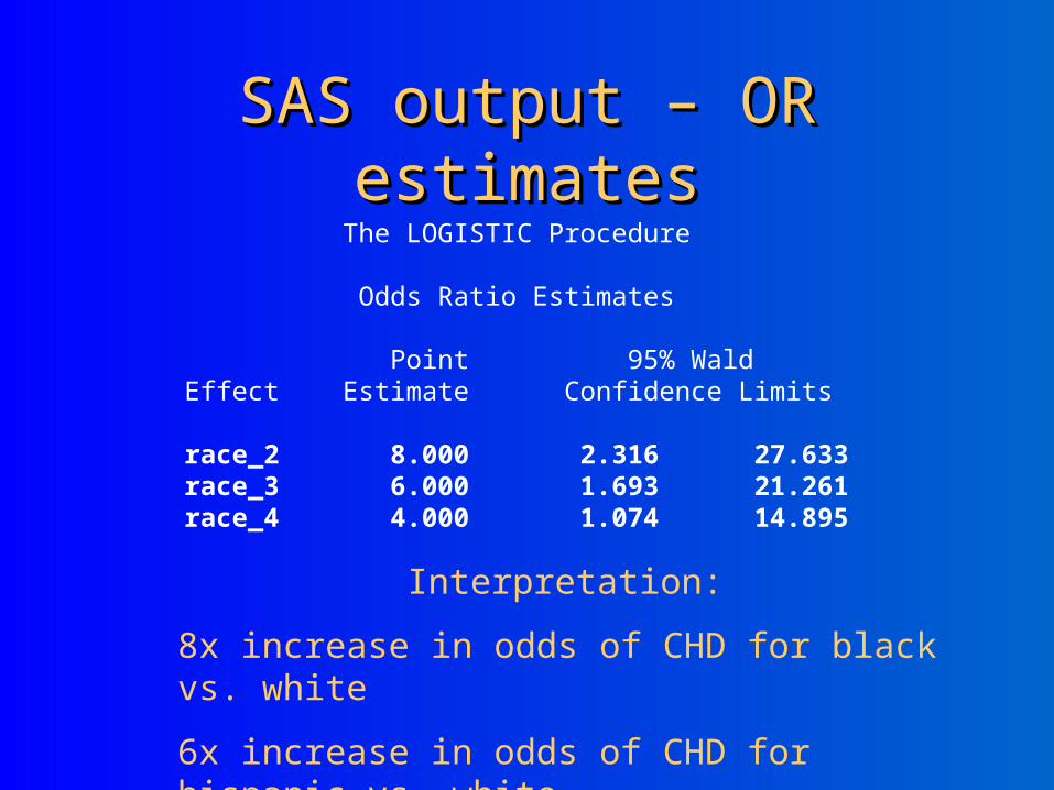
SAS output – OR estimatesSAS output – OR estimates The LOGISTIC Procedure  Odds Ratio Estimates  Point 95% Wald Effect Estimate Confidence Limits  race_2 8.000 2.316 27.633 race_3 6.000 1.693 21.261 race_4 4.000 1.074 14.895

Interpretation:

8x increase in odds of CHD for black vs. white

6x increase in odds of CHD for hispanic vs. white

4x increase in odds of CHD for other vs. white

Example 3: Prostrate Cancer Example 3: Prostrate Cancer StudyStudy

Question: Does PSA level predict tumor penetration into the prostatic capsule (yes/no)?

Is this association confounded by race?

Does race modify this association (interaction)?

1.1. What’s the relationship What’s the relationship between PSA (continuous between PSA (continuous variable) and capsule variable) and capsule penetration (binary)?penetration (binary)?

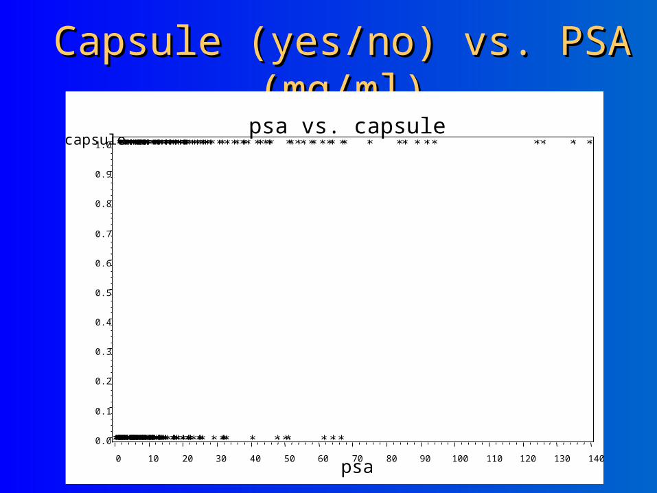
Capsule (yes/no) vs. PSA (mg/ml)Capsule (yes/no) vs. PSA (mg/ml)psa vs. capsule

capsule

0.0

0.1

0.2

0.3

0.4

0.5

0.6

0.7

0.8

0.9

1.0

psa0 10 20 30 40 50 60 70 80 90 100 110 120 130 140

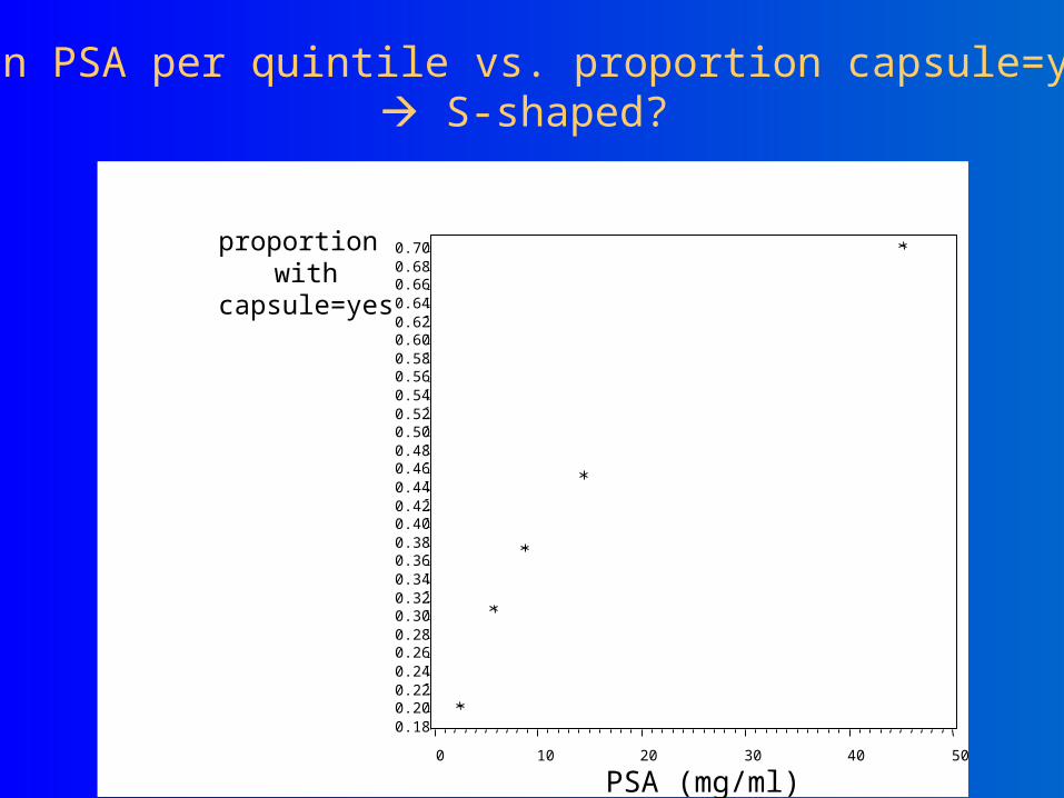
Mean PSA per quintile vs. proportion capsule=yes S-shaped?

proportion with

capsule=yes

0.180.200.220.240.260.280.300.320.340.360.380.400.420.440.460.480.500.520.540.560.580.600.620.640.660.680.70

PSA (mg/ml)0 10 20 30 40 50

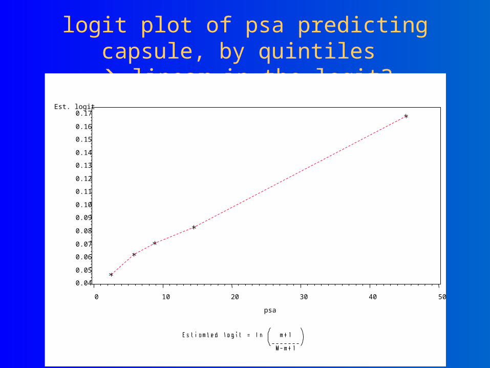
logit plot of psa predicting capsule, by quintiles

linear in the logit?Est. logit

0.04

0.05

0.06

0.07

0.08

0.09

0.10

0.11

0.12

0.13

0.14

0.15

0.16

0.17

psa

0 10 20 30 40 50

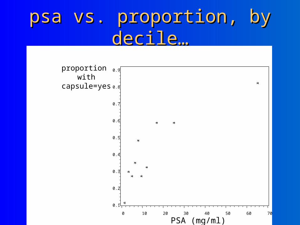
psa vs. proportion, by decile…psa vs. proportion, by decile…

0.1

0.2

0.3

0.4

0.5

0.6

0.7

0.8

0.9

0 10 20 30 40 50 60 70

proportion with

capsule=yes

PSA (mg/ml)

logit vs. psa, by decilelogit vs. psa, by decileEstimated logit plot of psa predicting capsule in the data set kristin.psa

m = numer of events M = number of cases

Est. logit

0.040.060.080.100.120.140.160.180.200.220.240.260.280.300.320.340.360.380.400.420.44

psa

0 10 20 30 40 50 60 70

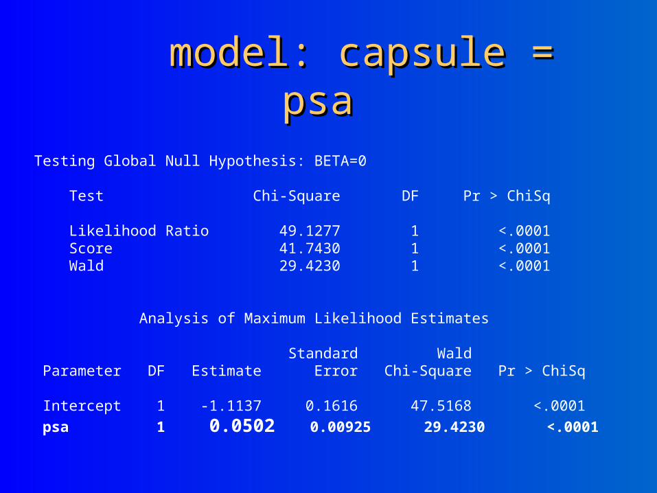
model: capsule = psamodel: capsule = psa  

Testing Global Null Hypothesis: BETA=0  Test Chi-Square DF Pr > ChiSq  Likelihood Ratio 49.1277 1 <.0001 Score 41.7430 1 <.0001 Wald 29.4230 1 <.0001   Analysis of Maximum Likelihood Estimates  Standard Wald Parameter DF Estimate Error Chi-Square Pr > ChiSq  Intercept 1 -1.1137 0.1616 47.5168 <.0001 psa 1 0.0502 0.00925 29.4230 <.0001

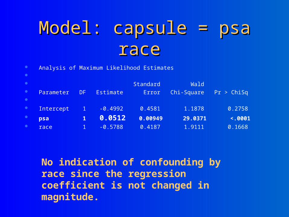
Model: capsule = psa raceModel: capsule = psa race Analysis of Maximum Likelihood Estimates   Standard Wald Parameter DF Estimate Error Chi-Square Pr > ChiSq   Intercept 1 -0.4992 0.4581 1.1878 0.2758 psa 1 0.0512 0.00949 29.0371 <.0001 race 1 -0.5788 0.4187 1.9111 0.1668

No indication of confounding by race since the regression coefficient is not changed in magnitude.

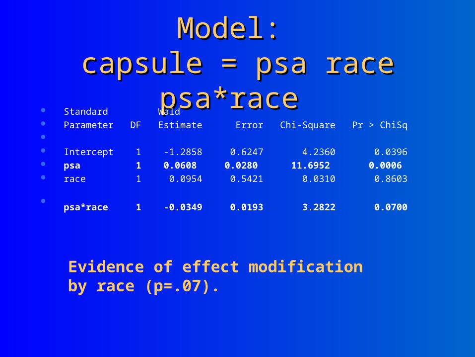
Model: Model: capsule = psa race psa*racecapsule = psa race psa*race

Standard Wald Parameter DF Estimate Error Chi-Square Pr > ChiSq   Intercept 1 -1.2858 0.6247 4.2360 0.0396 psa 1 0.0608 0.0280 11.6952 0.0006 race 1 0.0954 0.5421 0.0310 0.8603

psa*race 1 -0.0349 0.0193 3.2822 0.0700

Evidence of effect modification by race (p=.07).

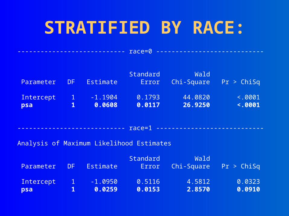
---------------------------- race=0 ---------------------------- 

Standard Wald Parameter DF Estimate Error Chi-Square Pr > ChiSq  Intercept 1 -1.1904 0.1793 44.0820 <.0001 psa 1 0.0608 0.0117 26.9250 <.0001  ---------------------------- race=1 ---------------------------- Analysis of Maximum Likelihood Estimates  Standard Wald Parameter DF Estimate Error Chi-Square Pr > ChiSq  Intercept 1 -1.0950 0.5116 4.5812 0.0323 psa 1 0.0259 0.0153 2.8570 0.0910

STRATIFIED BY RACE:

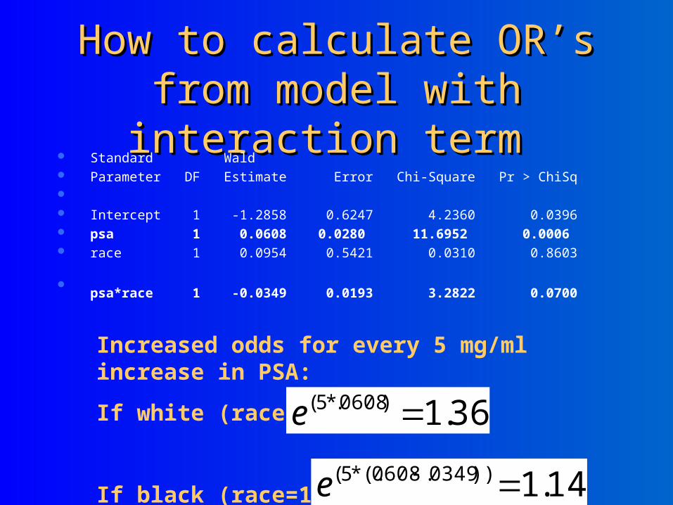
How to calculate OR’s from How to calculate OR’s from model with interaction termmodel with interaction term

Standard Wald Parameter DF Estimate Error Chi-Square Pr > ChiSq   Intercept 1 -1.2858 0.6247 4.2360 0.0396 psa 1 0.0608 0.0280 11.6952 0.0006 race 1 0.0954 0.5421 0.0310 0.8603

psa*race 1 -0.0349 0.0193 3.2822 0.0700

Increased odds for every 5 mg/ml increase in PSA:

If white (race=0):

If black (race=1):

36.1)0608.*5( e

14.1))0349.0608*(.5( e

Example 4: Model buildingExample 4: Model buildingand the prostate cancer studyand the prostate cancer study

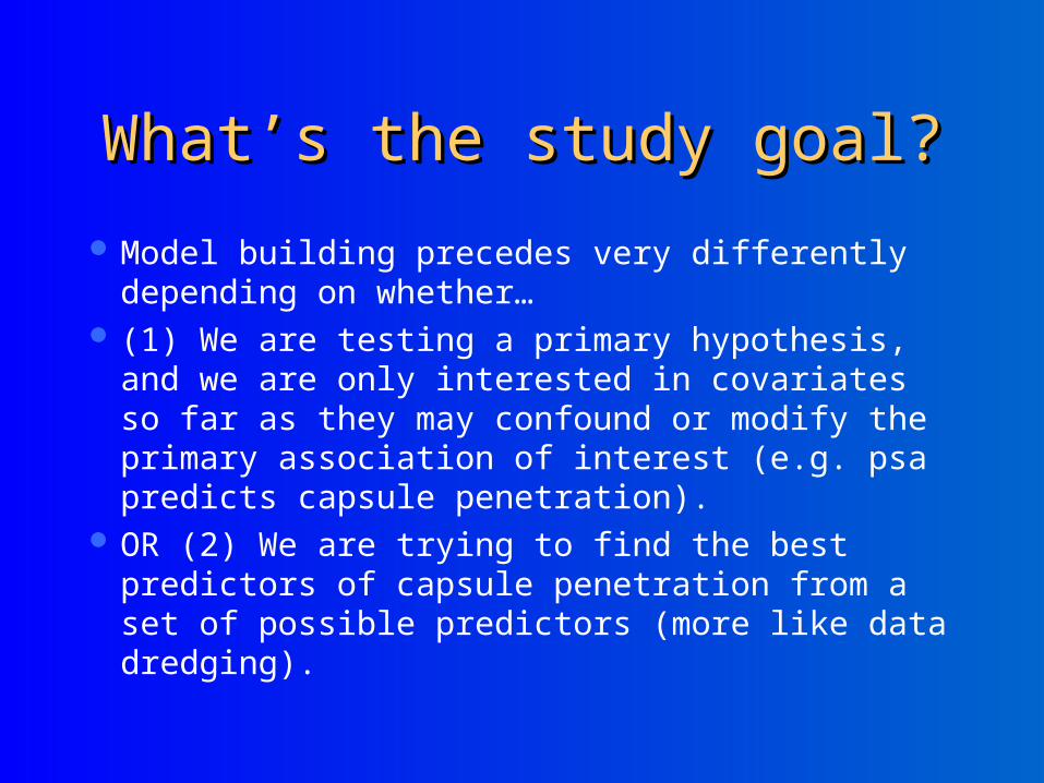
What’s the study goal?What’s the study goal?

Model building precedes very differently depending on whether…

(1) We are testing a primary hypothesis, and we are only interested in covariates so far as they may confound or modify the primary association of interest (e.g. psa predicts capsule penetration).

OR (2) We are trying to find the best predictors of capsule penetration from a set of possible predictors (more like data dredging).

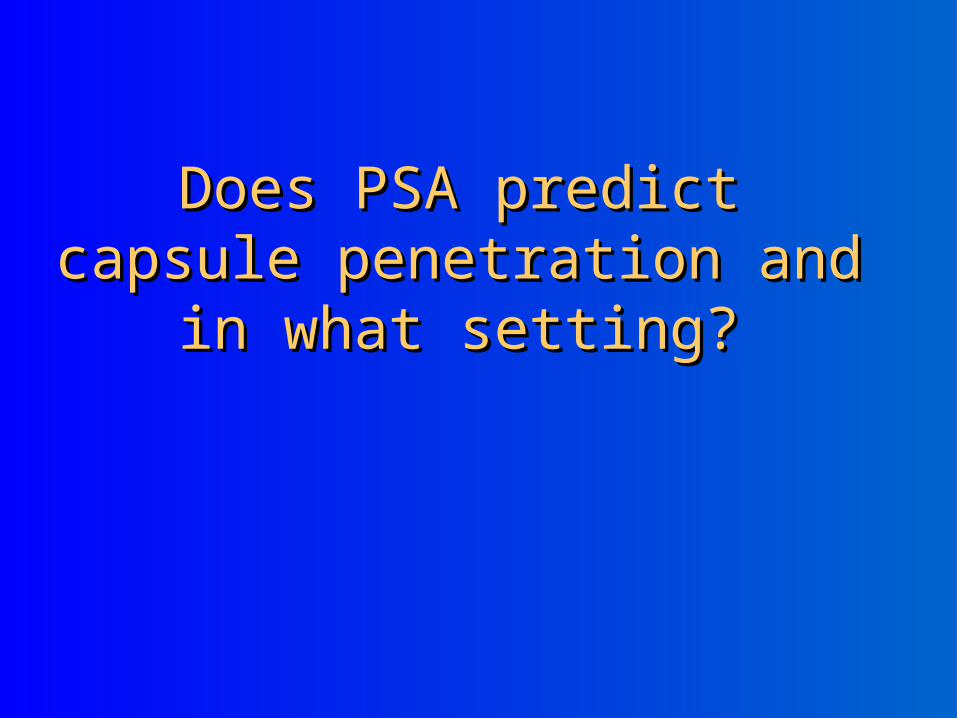
Does PSA predict capsule Does PSA predict capsule penetration and in what setting?penetration and in what setting?

Univariate analysisUnivariate analysis

Other variables in the dataset that we are going to consider today (besides race, psa):

Age Tumor Volume (from ultrasound) Total Gleason Score, 0 - 10

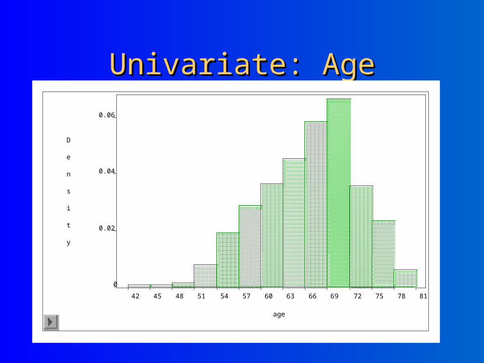
Univariate: AgeUnivariate: Age

42 45 48 51 54 57 60 63 66 69 72 75 78 81

age

0

0.02

0.04

0.06

D

e

n

s

i

t

y

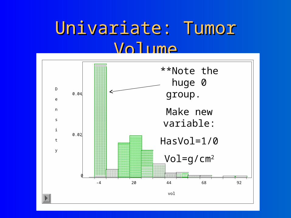
Univariate: Tumor VolumeUnivariate: Tumor Volume

-4 20 44 68 92

vol

0

0.02

0.04D

e

n

s

i

t

y

**Note the huge 0 group.

Make new variable:

HasVol=1/0

Vol=g/cm2

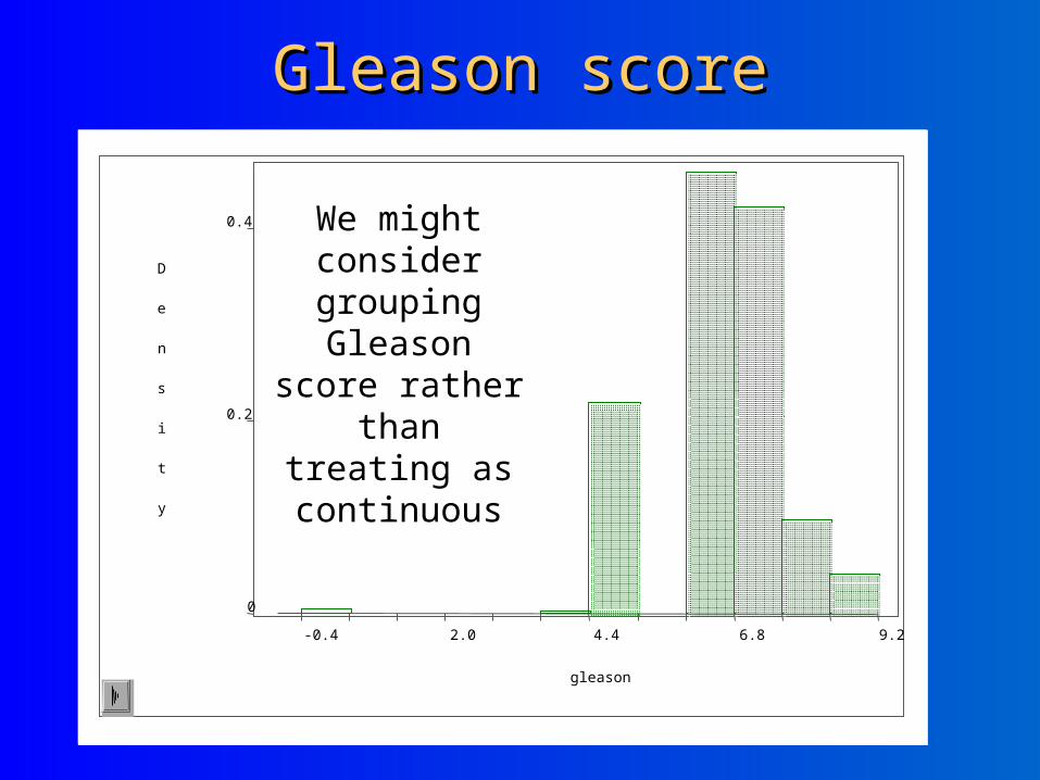
Gleason scoreGleason score

-0.4 2.0 4.4 6.8 9.2

gleason

0

0.2

0.4

D

e

n

s

i

t

y

We might consider grouping

Gleason score rather than treating as continuous

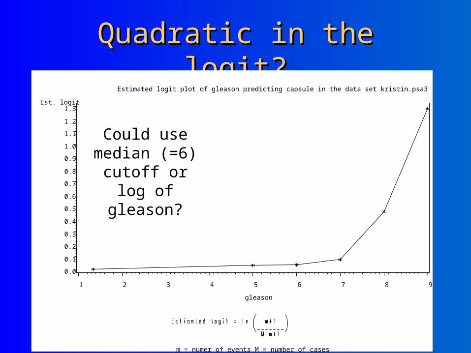
Quadratic in the logit?Quadratic in the logit?Estimated logit plot of gleason predicting capsule in the data set kristin.psa3

m = numer of events M = number of cases

Est. logit

0.0

0.1

0.2

0.3

0.4

0.5

0.6

0.7

0.8

0.9

1.0

1.1

1.2

1.3

gleason

1 2 3 4 5 6 7 8 9

Could use median (=6) cutoff or log

of gleason?

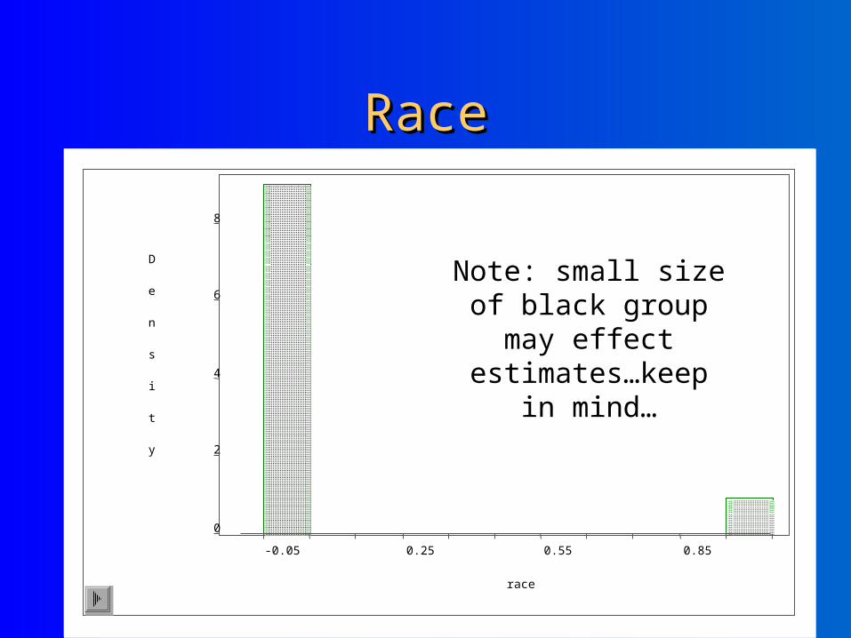
RaceRace

-0.05 0.25 0.55 0.85

race

0

2

4

6

8

D

e

n

s

i

t

y

Note: small size of black group may effect

estimates…keep in mind…

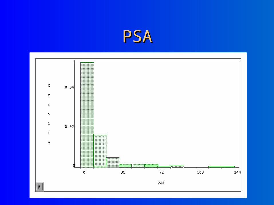
PSAPSA

0 36 72 108 144

psa

0

0.02

0.04D

e

n

s

i

t

y

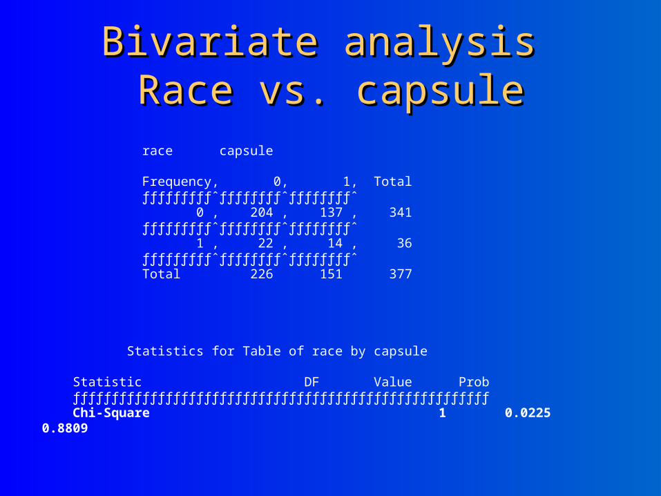
Bivariate analysis Bivariate analysis Race vs. capsuleRace vs. capsule

   race capsule  Frequency‚ 0‚ 1‚ Total ƒƒƒƒƒƒƒƒƒˆƒƒƒƒƒƒƒƒˆƒƒƒƒƒƒƒƒˆ 0 ‚ 204 ‚ 137 ‚ 341 ƒƒƒƒƒƒƒƒƒˆƒƒƒƒƒƒƒƒˆƒƒƒƒƒƒƒƒˆ 1 ‚ 22 ‚ 14 ‚ 36 ƒƒƒƒƒƒƒƒƒˆƒƒƒƒƒƒƒƒˆƒƒƒƒƒƒƒƒˆ Total 226 151 377     Statistics for Table of race by capsule  Statistic DF Value Prob ƒƒƒƒƒƒƒƒƒƒƒƒƒƒƒƒƒƒƒƒƒƒƒƒƒƒƒƒƒƒƒƒƒƒƒƒƒƒƒƒƒƒƒƒƒƒƒƒƒƒƒƒƒƒ Chi-Square 1 0.0225 0.8809

Bivariate analysis Bivariate analysis Age and capsuleAge and capsule

  Analysis of Maximum Likelihood Estimates   Standard Wald Parameter DF Estimate Error Chi-Square Pr > ChiSq   Intercept 1 -0.1491 1.0623 0.0197 0.8884 age 1 0.00824 0.0160 0.2642 0.6073

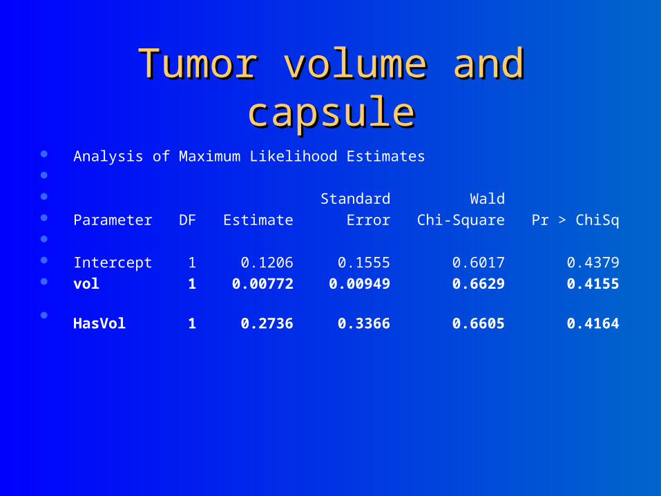
Tumor volume and capsuleTumor volume and capsule

Analysis of Maximum Likelihood Estimates   Standard Wald Parameter DF Estimate Error Chi-Square Pr > ChiSq   Intercept 1 0.1206 0.1555 0.6017 0.4379 vol 1 0.00772 0.00949 0.6629 0.4155

HasVol 1 0.2736 0.3366 0.6605 0.4164

Gleason score and capsuleGleason score and capsule

Analysis of Maximum Likelihood Estimates  Standard Wald Parameter DF Estimate Error Chi-Square Pr > ChiSq  Intercept 1 8.4196 1.0024 70.5458 <.0001 gleason 1 -1.2388 0.1526 65.9389 <.0001

SummarySummary

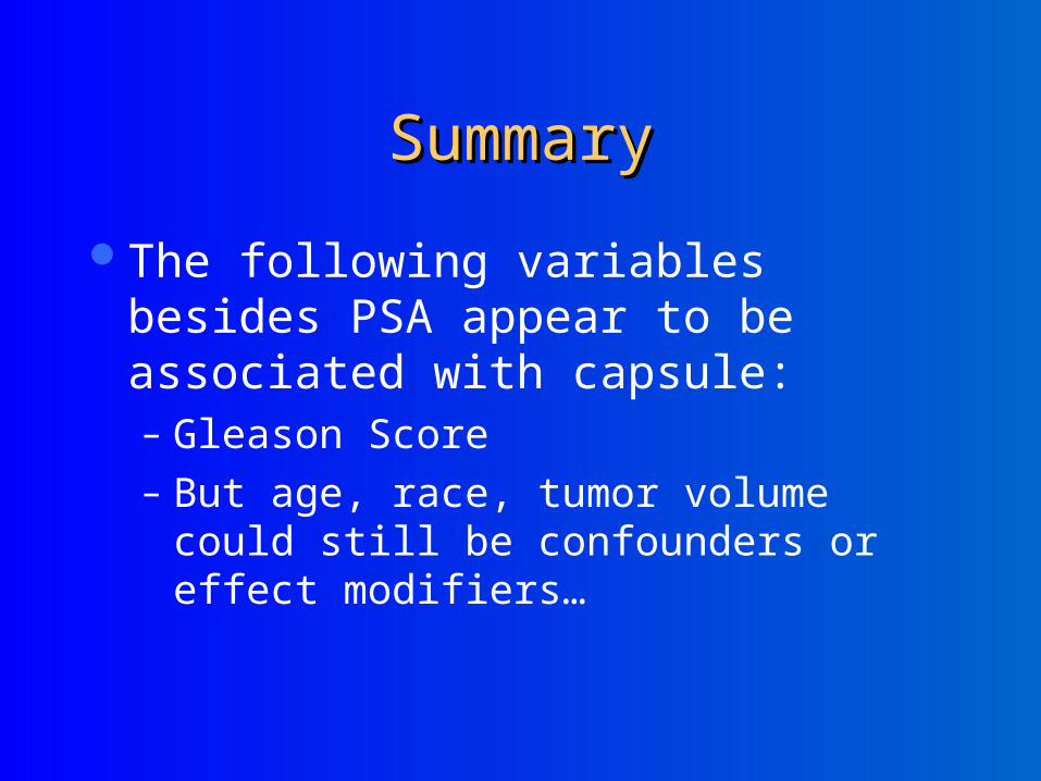
The following variables besides PSA appear to be associated with capsule:– Gleason Score– But age, race, tumor volume could still be

confounders or effect modifiers…

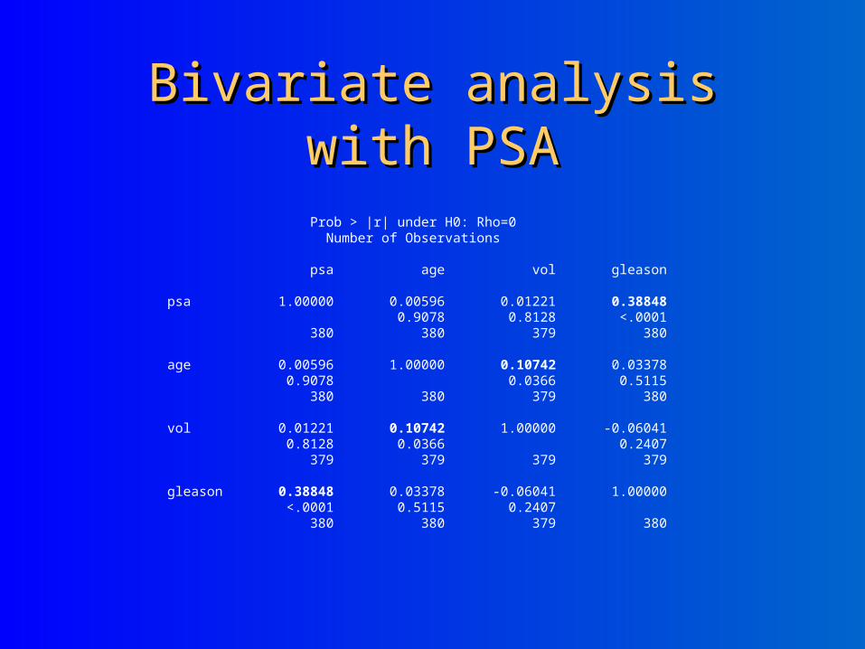
Bivariate analysis with PSABivariate analysis with PSA

Prob > |r| under H0: Rho=0 Number of Observations  psa age vol gleason psa 1.00000 0.00596 0.01221 0.38848 0.9078 0.8128 <.0001 380 380 379 380 age 0.00596 1.00000 0.10742 0.03378 0.9078 0.0366 0.5115 380 380 379 380 vol 0.01221 0.10742 1.00000 -0.06041 0.8128 0.0366 0.2407 379 379 379 379 gleason 0.38848 0.03378 -0.06041 1.00000 <.0001 0.5115 0.2407 380 380 379 380

HasVol vs. PSAHasVol vs. PSA

  Lower CL Upper CL Variable HasVol N Mean Mean Mean  psa Diff (1-2) -2.952 1.1272 5.2062  T-Tests Variable Method Variances DF t Value Pr > |t| psa Pooled Equal 377 0.54 0.5872psa Satterthwaite Unequal 357 0.54 0.5865

Race (white/black) vs. PSARace (white/black) vs. PSA

PSA vs. race Lower CL Upper CL Variable race N Mean Mean Mean  psa Diff (1-2) -17.15 -10.38 -3.603  Variable Method Variances DF t Value Pr > |t| psa Pooled Equal 375 -3.01 0.0028psa Satterthwaite Unequal 38.6 -2.23 0.0313

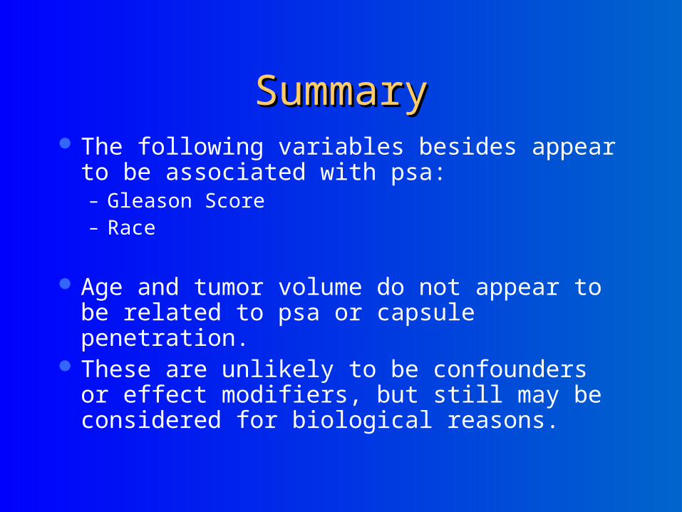
SummarySummary The following variables besides appear to be

associated with psa:– Gleason Score– Race

Age and tumor volume do not appear to be related to psa or capsule penetration.

These are unlikely to be confounders or effect modifiers, but still may be considered for biological reasons.

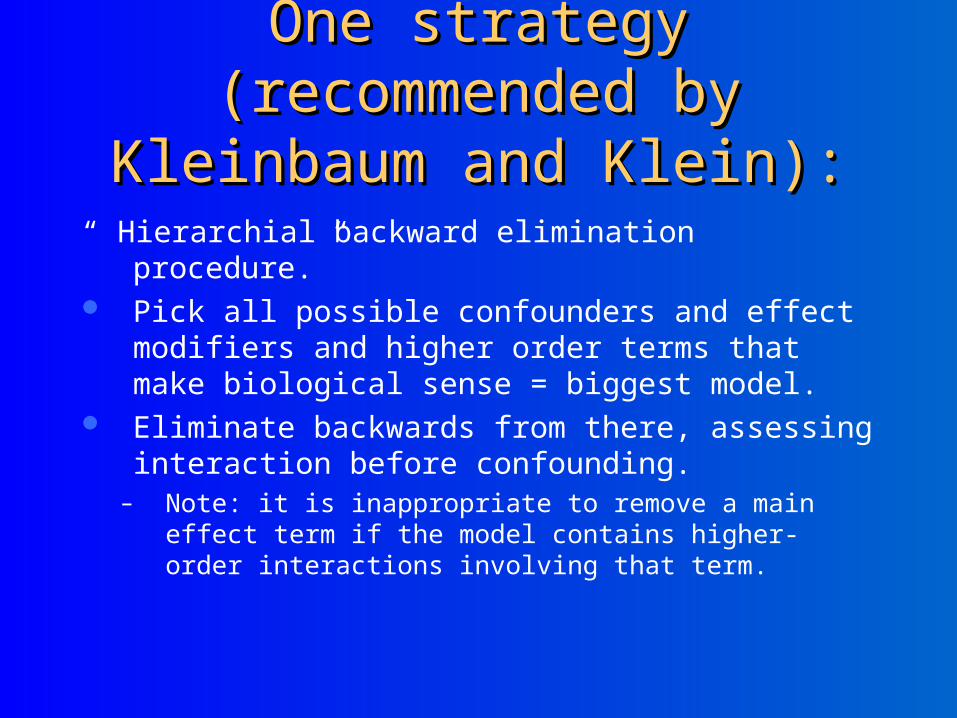
One strategy (recommended One strategy (recommended by Kleinbaum and Klein):by Kleinbaum and Klein):

“ Hierarchial backward elimination procedure.” Pick all possible confounders and effect

modifiers and higher order terms that make biological sense = biggest model.

Eliminate backwards from there, assessing interaction before confounding.

– Note: it is inappropriate to remove a main effect term if the model contains higher-order interactions involving that term.

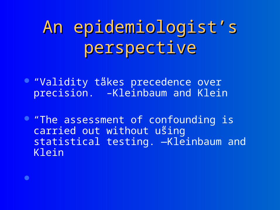
An epidemiologist’s An epidemiologist’s perspectiveperspective

“Validity takes precedence over precision.” –Kleinbaum and Klein

“The assessment of confounding is carried out without using statistical testing.”—Kleinbaum and Klein

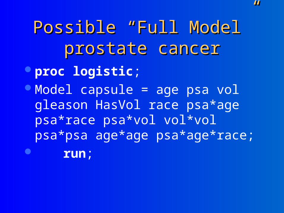
Possible “Full Model” prostate Possible “Full Model” prostate cancercancer

proc logistic;Model capsule = age psa vol gleason

HasVol race psa*age psa*race psa*vol vol*vol psa*psa age*age psa*age*race;

run;

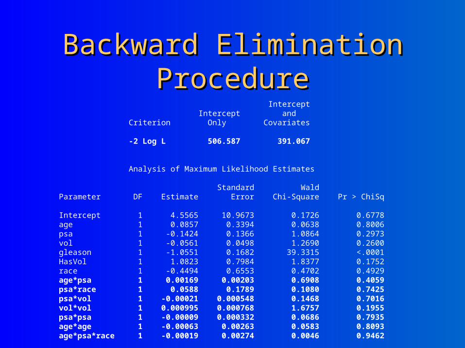
Backward Elimination Backward Elimination ProcedureProcedure

Intercept Intercept and Criterion Only Covariates  -2 Log L 506.587 391.067    Analysis of Maximum Likelihood Estimates  Standard WaldParameter DF Estimate Error Chi-Square Pr > ChiSq Intercept 1 4.5565 10.9673 0.1726 0.6778age 1 0.0857 0.3394 0.0638 0.8006psa 1 -0.1424 0.1366 1.0864 0.2973vol 1 -0.0561 0.0498 1.2690 0.2600gleason 1 -1.0551 0.1682 39.3315 <.0001HasVol 1 1.0823 0.7984 1.8377 0.1752race 1 -0.4494 0.6553 0.4702 0.4929age*psa 1 0.00169 0.00203 0.6908 0.4059psa*race 1 0.0588 0.1789 0.1080 0.7425psa*vol 1 -0.00021 0.000548 0.1468 0.7016vol*vol 1 0.000995 0.000768 1.6757 0.1955psa*psa 1 -0.00009 0.000332 0.0686 0.7935age*age 1 -0.00063 0.00263 0.0583 0.8093age*psa*race 1 -0.00019 0.00274 0.0046 0.9462

subtracting away all the interaction and higher order terms...the model fit is...  Intercept Intercept and Criterion Only Covariates 

-2 Log L 506.587 396.894

LRtest= 396.8 (reduced model) – 391(full model) = 5.8; chi-square of 7 df. NS.What Kleinbaum and Klein call the “Chunk Test.”

Many, many other strategies are possible…eliminate one at a timeas Agresti talks about (highest p-value first)Hosmer and Lemeshow put all main effects in the model and try interaction terms one at a time, keeping only those that are significantI.e., many possible strategies!! No one right answer…I’m choosing the one that saves class time!Less desirable automated computer selection

Model capsule = age psa vol gleason HasVol race

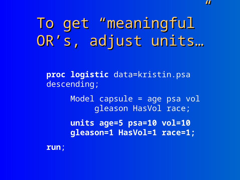
proc logistic data=kristin.psa descending;

Model capsule = age psa vol gleason HasVol race;

units age=5 psa=10 vol=10 gleason=1 HasVol=1 race=1;

run;

To get “meaningful” OR’s, To get “meaningful” OR’s, adjust units…adjust units…

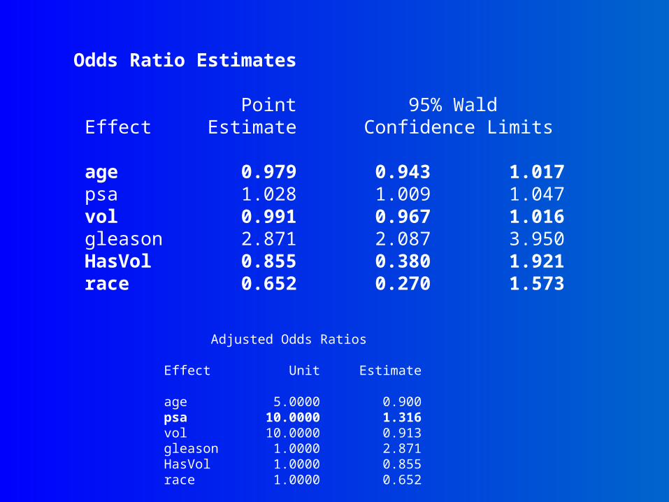
Odds Ratio Estimates  Point 95% Wald Effect Estimate Confidence Limits  age 0.979 0.943 1.017 psa 1.028 1.009 1.047 vol 0.991 0.967 1.016 gleason 2.871 2.087 3.950 HasVol 0.855 0.380 1.921 race 0.652 0.270 1.573

Adjusted Odds Ratios  Effect Unit Estimate  age 5.0000 0.900 psa 10.0000 1.316 vol 10.0000 0.913 gleason 1.0000 2.871 HasVol 1.0000 0.855 race 1.0000 0.652

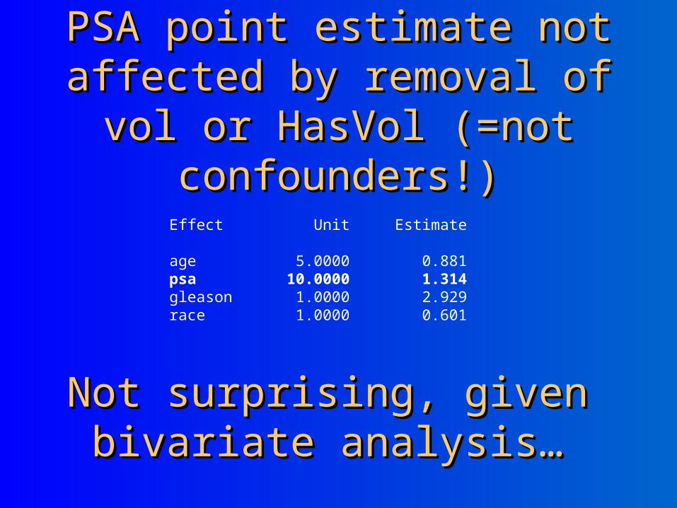
PSA point estimate not PSA point estimate not affected by removal of vol or affected by removal of vol or HasVol (=not confounders!)HasVol (=not confounders!)

  Effect Unit Estimate  age 5.0000 0.881 psa 10.0000 1.314 gleason 1.0000 2.929 race 1.0000 0.601

Not surprising, given bivariate Not surprising, given bivariate analysis…analysis…

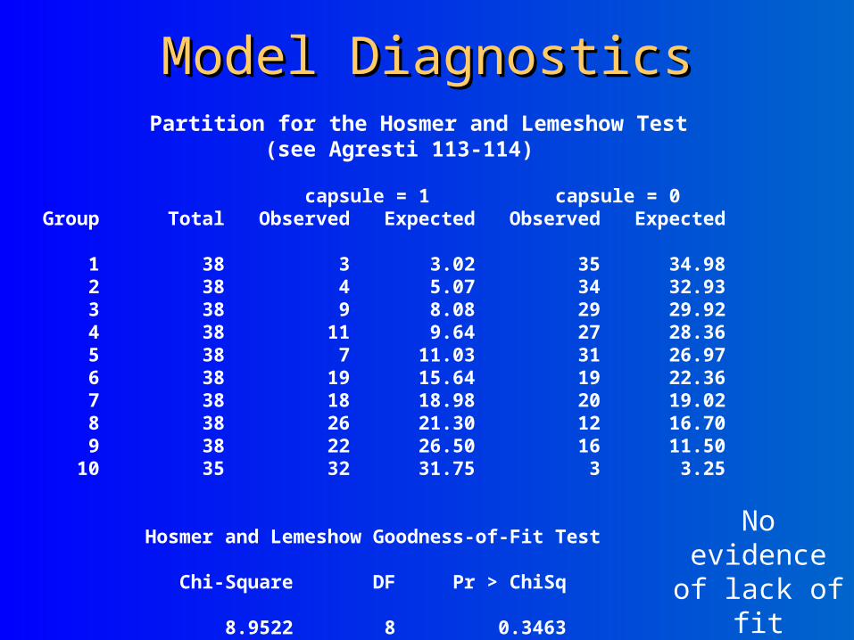
Model DiagnosticsModel Diagnostics Partition for the Hosmer and Lemeshow Test

(see Agresti 113-114)  capsule = 1 capsule = 0 Group Total Observed Expected Observed Expected  1 38 3 3.02 35 34.98 2 38 4 5.07 34 32.93 3 38 9 8.08 29 29.92 4 38 11 9.64 27 28.36 5 38 7 11.03 31 26.97 6 38 19 15.64 19 22.36 7 38 18 18.98 20 19.02 8 38 26 21.30 12 16.70 9 38 22 26.50 16 11.50 10 35 32 31.75 3 3.25   Hosmer and Lemeshow Goodness-of-Fit Test  Chi-Square DF Pr > ChiSq  8.9522 8 0.3463

No evidence of lack of

fit

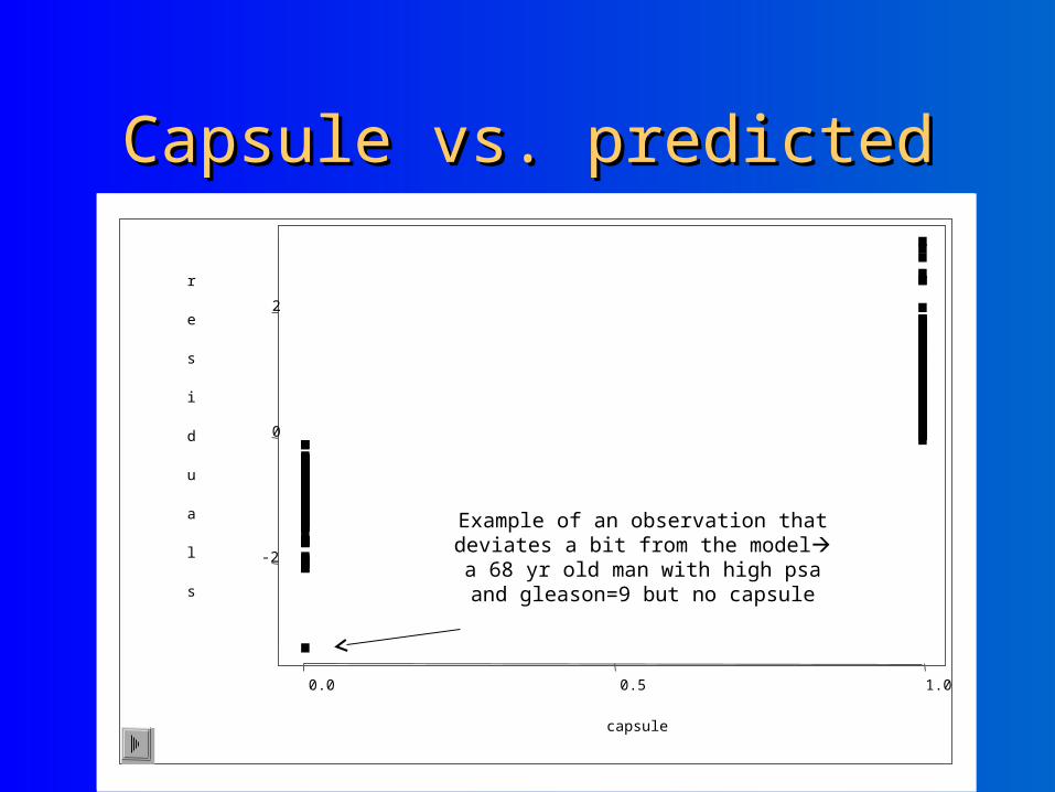
Capsule vs. predictedCapsule vs. predicted

0.0 0.5 1.0

capsule

-2

0

2

r

e

s

i

d

u

a

l

s

Example of an observation that deviates a bit from the model a 68 yr old man with high psa and gleason=9 but no capsule

DiscussionDiscussion

What are some of the merits of the preceding model selection procedure?

What are some problems that you see?– e.g. What happened to race*psa interaction?

Model building is an art!

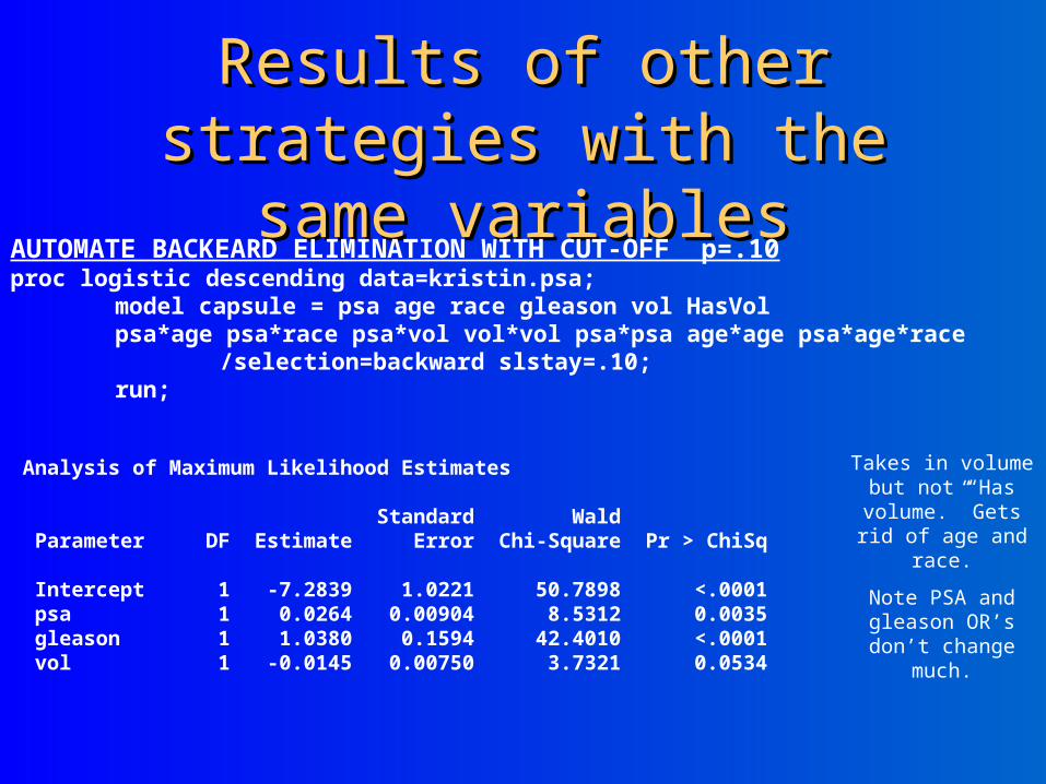
Results of other strategies Results of other strategies with the same variableswith the same variables

AUTOMATE BACKEARD ELIMINATION WITH CUT-OFF p=.10proc logistic descending data=kristin.psa;

model capsule = psa age race gleason vol HasVol psa*age psa*race psa*vol vol*vol psa*psa age*age psa*age*race

/selection=backward slstay=.10;run;

Analysis of Maximum Likelihood Estimates  Standard Wald Parameter DF Estimate Error Chi-Square Pr > ChiSq  Intercept 1 -7.2839 1.0221 50.7898 <.0001 psa 1 0.0264 0.00904 8.5312 0.0035 gleason 1 1.0380 0.1594 42.4010 <.0001 vol 1 -0.0145 0.00750 3.7321 0.0534

Takes in volume but not “Has volume.” Gets rid of age and

race.

Note PSA and gleason OR’s don’t change

much.

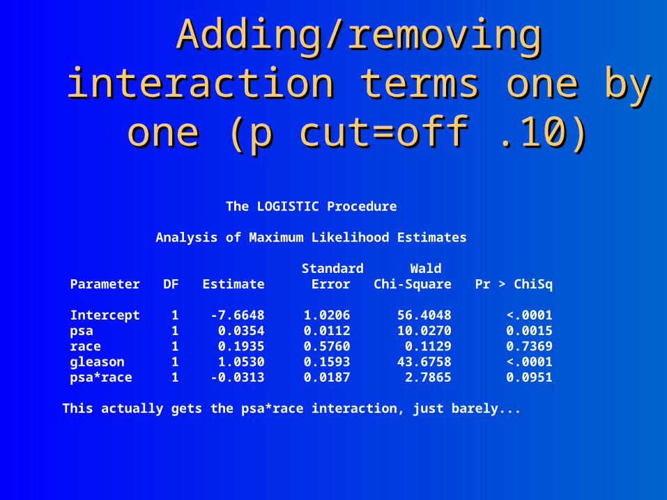
Adding/removing interaction Adding/removing interaction terms one by one (p cut=off .10)terms one by one (p cut=off .10)

The LOGISTIC Procedure  Analysis of Maximum Likelihood Estimates  Standard Wald Parameter DF Estimate Error Chi-Square Pr > ChiSq  Intercept 1 -7.6648 1.0206 56.4048 <.0001 psa 1 0.0354 0.0112 10.0270 0.0015 race 1 0.1935 0.5760 0.1129 0.7369 gleason 1 1.0530 0.1593 43.6758 <.0001 psa*race 1 -0.0313 0.0187 2.7865 0.0951

This actually gets the psa*race interaction, just barely...

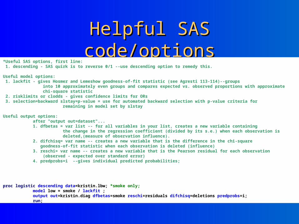
Helpful SAS code/optionsHelpful SAS code/options*Useful SAS options, first line: 1. descending - SAS quirk is to reverse 0/1 --use descending option to remedy this. Useful model options: 1. lackfit - gives Hosmer and Lemeshow goodness-of-fit statistic (see Agresti 113-114)--groups

into 10 approximately even groups and compares expected vs. observed proportions with approximate chi-square statistic

2. risklimits or clodds - gives confidence limits for ORs 3. selection=backward slstay=p-value = use for automated backward selection with p-value criteria for

remaining in model set by slstay Useful output options:

after "output out=dataset"...1. dfbetas = var list -- for all variables in your list, creates a new variable containing

the change in the regression coefficient (divided by its s.e.) when each observation is deleted,(measure of observation influence).

2. difchisq= var name -- creates a new variable that is the difference in the chi-square goodness-of-fit statistic when each observation is deleted (influence)3. reschi= var name -- creates a new variable that is the Pearson residual for each observation (observed - expected over standard error)4. predprobs=i --gives individual predicted probabilities;

EXAMPLE”

proc logistic descending data=kristin.lbw; *smoke only;model low = smoke / lackfit ;output out=kristin.diag dfbetas=smoke reschi=residuals difchisq=deletions predprobs=i;run;