Logistic Regression ILogistic Regression I

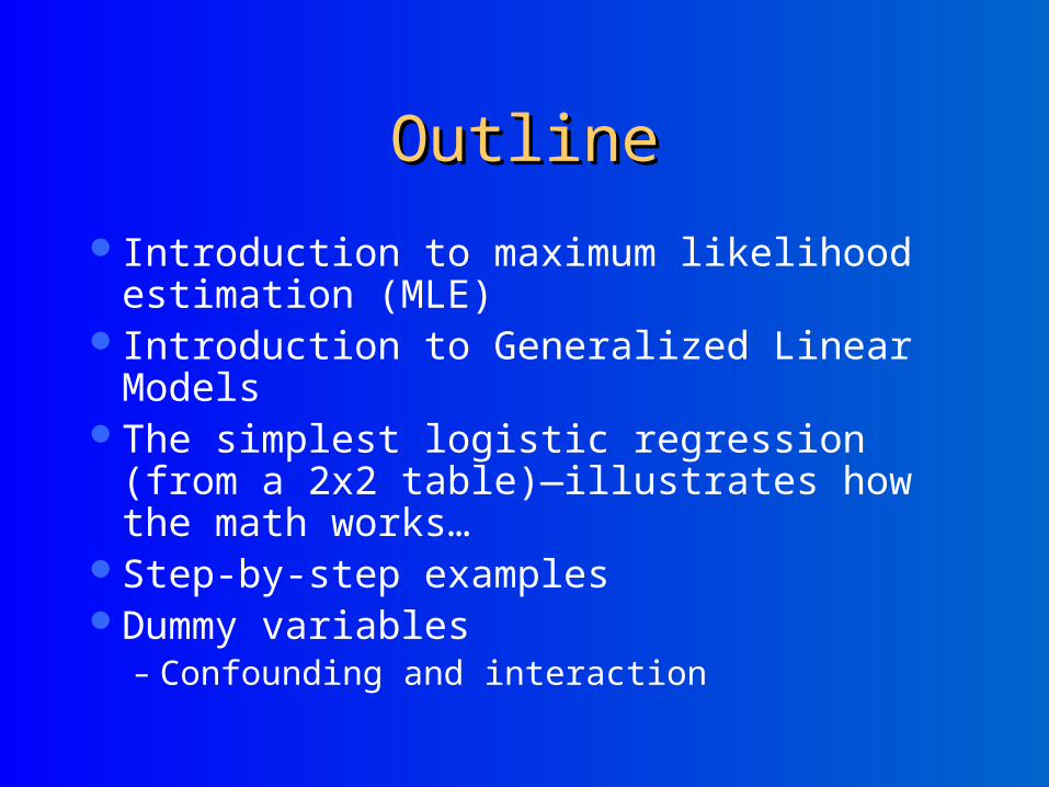
OutlineOutline

Introduction to maximum likelihood estimation (MLE)

Introduction to Generalized Linear ModelsThe simplest logistic regression (from a 2x2

table)—illustrates how the math works…Step-by-step examples Dummy variables

– Confounding and interaction

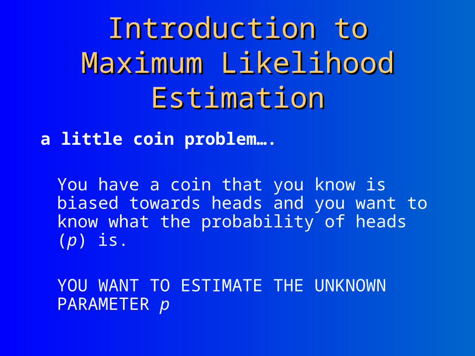
Introduction to Maximum Introduction to Maximum Likelihood EstimationLikelihood Estimation

a little coin problem…. 

You have a coin that you know is biased towards heads and you want to know what the probability of heads (p) is.

YOU WANT TO ESTIMATE THE UNKNOWN PARAMETER p  

DataData

You flip the coin 10 times and the coin comes up heads 7 times. What’s you’re best guess for p?

 

Can we agree that your best guess for is .7 based on the data?

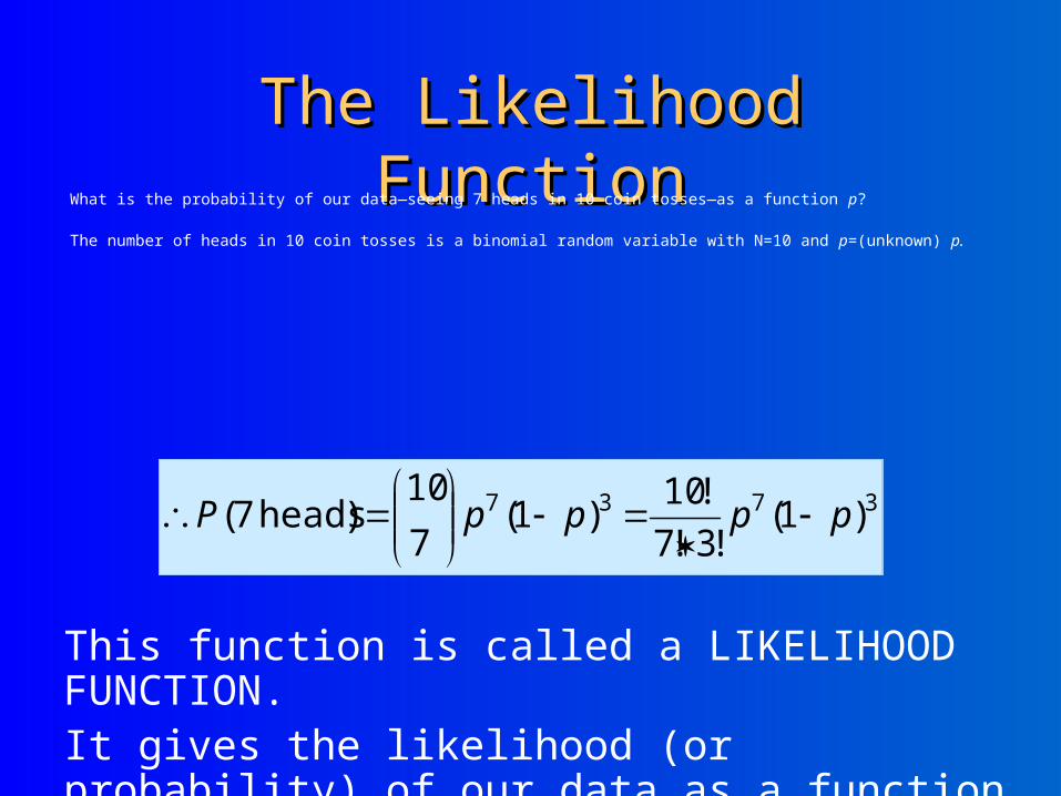
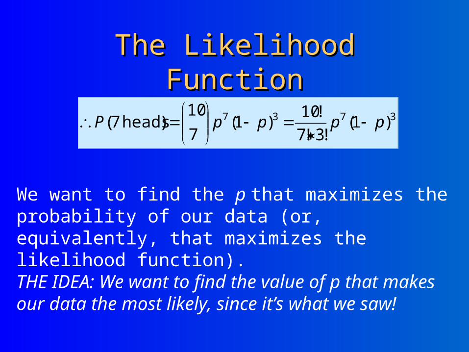
The Likelihood FunctionThe Likelihood FunctionWhat is the probability of our data—seeing 7 heads in 10 coin tosses—as a function p?

The number of heads in 10 coin tosses is a binomial random variable with N=10 and p=(unknown) p.

 

3737 )1(!3!7

!10)1(

7

10)heads 7( ppppP

This function is called a LIKELIHOOD FUNCTION.It gives the likelihood (or probability) of our data as a function of our unknown parameter p.

The Likelihood FunctionThe Likelihood Function

3737 )1(!3!7

!10)1(

7

10)heads 7( ppppP

We want to find the p that maximizes the probability of our data (or, equivalently, that maximizes the likelihood function). THE IDEA: We want to find the value of p that makes our data the most likely, since it’s what we saw!

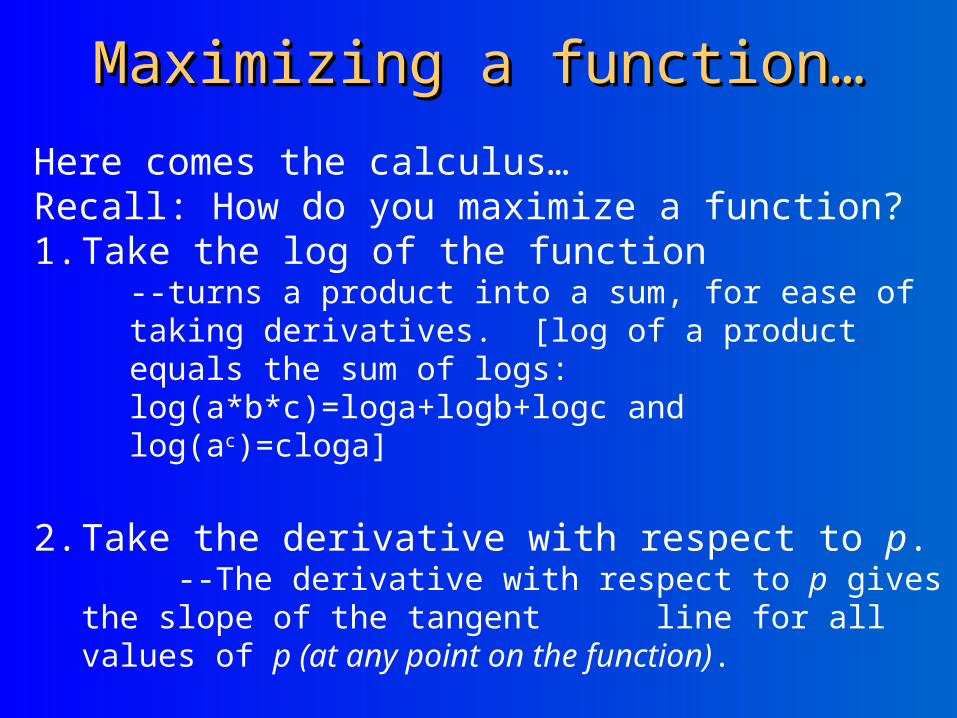
Maximizing a function…Maximizing a function…

Here comes the calculus…Recall: How do you maximize a function? 1. Take the log of the function

--turns a product into a sum, for ease of taking derivatives. [log of a product equals the sum of logs: log(a*b*c)=loga+logb+logc and log(ac)=cloga]

2. Take the derivative with respect to p. --The derivative with respect to p gives the slope of the

tangent line for all values of p (at any point on the function).

3. Set the derivative equal to 0 and solve for p. --Find the value of p where the slope of the tangent line is 0

— this is a horizontal line, so must occur at the peak or the trough.

1. Take the log of the likelihood function.

)1log(3log7!3!7

!10loglog ppLikelihood

3. Set the derivative equal to 0 and solve for p.

2. Take the derivative with respect to p.

ppLikelihood

dp

d

1

370log

10

7

107377

3)1(70)1(

3)1(70

1

37

p

ppp

pppp

pp

pp

Jog your memory

*derivative of a constant is 0

*derivative 7f(x)=7f '(x)

*derivative of log x is 1/x

*chain rule

3737 )1(!3!7

!10)1(

7

10ppppLikelihood

10

7

107

377

3)1(7

0)1(

3)1(7

01

37

1

370log

)1log(3log7!3!7

!10loglog

p

p

pp

pp

pp

pp

pp

ppLikelihood

dp

d

ppLikelihood

267.)3(.)7(.120)3(.)7(.7

10Likelihood theof Value 3737

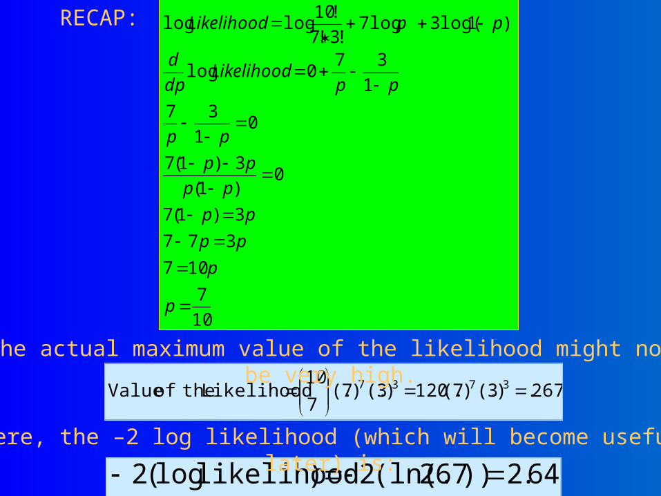
The actual maximum value of the likelihood might not be very high.

RECAP:

64.2))267(ln(.2)likelihood log(2 Here, the –2 log likelihood (which will become useful later) is:

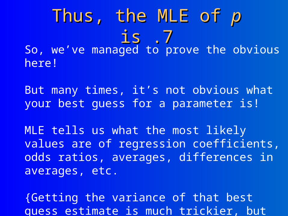
Thus, the MLE of Thus, the MLE of pp is .7 is .7So, we’ve managed to prove the obvious here!

But many times, it’s not obvious what your best guess for a parameter is!

MLE tells us what the most likely values are of regression coefficients, odds ratios, averages, differences in averages, etc.

{Getting the variance of that best guess estimate is much trickier, but it’s based on the second derivative, for another time ;-) }

GeneralGeneralized ized Linear ModelsLinear Models

Twice the generality!The generalized linear model is a

generalization of the general linear modelSAS uses PROC GLM for general linear

models SAS uses PROC GENMOD for generalized

linear models

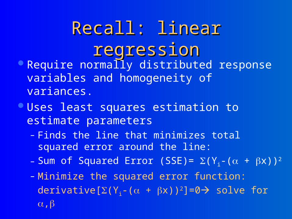
Recall: linear regressionRecall: linear regressionRequire normally distributed response variables

and homogeneity of variances. Uses least squares estimation to estimate

parameters– Finds the line that minimizes total squared error

around the line:

– Sum of Squared Error (SSE)= (Yi-( + x))2

– Minimize the squared error function:

derivative[(Yi-( + x))2]=0 solve for ,

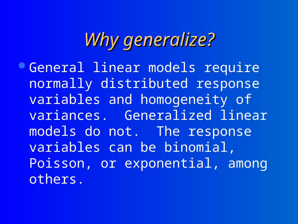
Why generalize?Why generalize?General linear models require normally

distributed response variables and homogeneity of variances. Generalized linear models do not. The response variables can be binomial, Poisson, or exponential, among others.

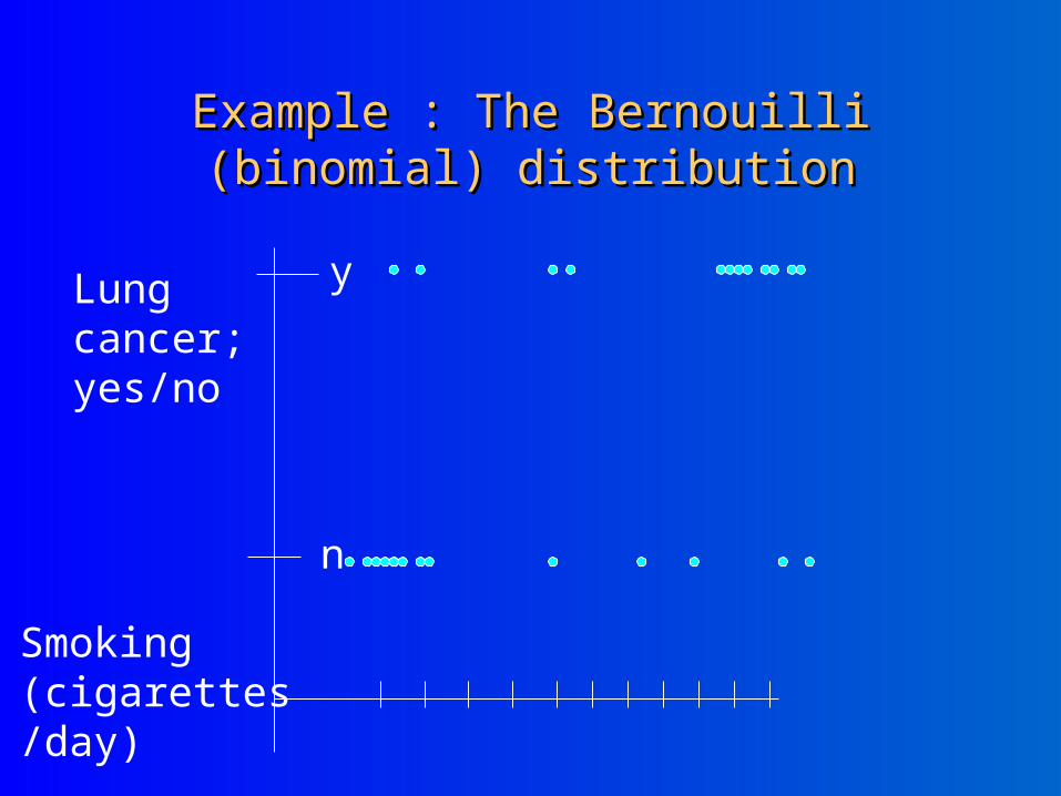
Example : The Bernouilli (binomial) Example : The Bernouilli (binomial) distributiondistribution

Smoking (cigarettes/day)

Lung cancer; yes/no

y

n

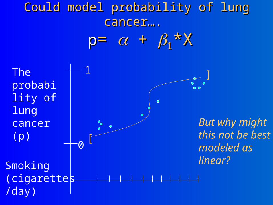
Could model probability of lung Could model probability of lung cancer…. cancer….

pp= = + + 11*X*X

Smoking (cigarettes/day)

The probability of lung cancer (p)

1

0

But why might this not be best modeled as linear?

[

]

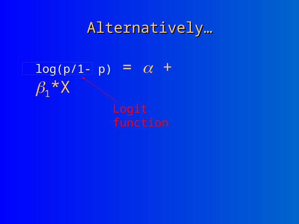
Alternatively…Alternatively…

log(p/1- p) = + 1*X

Logit function

The Logit ModelThe Logit Model

),())/(1

)/(ln( βX

X

Xi

i

i rDP

DP

Logit function (log odds)Baseline odds

Linear function of risk factors and covariates for individual i:

1x1 + 2x2 + 3x3 + 4x4

…

Bolded variables represent vectors

ExampleExample

)1()140()23()lbs) 140 old; years 23 ;P(D/smokes1

lbs) 140 old; years 23 ;P(D/smokesln( smokeweightage

Baseline odds

Linear function of risk factors and covariates for individual i:

1x1 + 2x2 + 3x3 + 4x4

…

Logit function (log odds of disease or outcome)

)1()140()23(

lbs) 140 old; years 23 ;P(D/smokes1

lbs) 140 old; years 23 ;P(D/smokes

smoker... lb,-140 old,year -23for disease of odds

smokeweightagee

Relating odds to probabilitiesRelating odds to probabilities

)(

)(

),(

1)/(

)/(1

)/(

),()()/()/(

),()/(

),()/(

onmanipulati algebraic

βX

βX

i

βX

i

i

i

i

βiXβiX

iXiX

βiX

iXβiX

iX

i

X

X

X

,r

,r

r

e

eDP

eDP

DP

re

,reDPDP

reDP

reDP

odds

algebra

probability

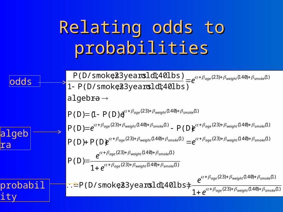
)1()140()23(

)1()140()23(

)1()140()23(

)1()140()23(

)1()140()23()1()140()23(

)1()140()23()1()140()23(

)1()140()23(

)1()140()23(

1lbs) 140 old; years 23 ;P(D/smokes

1P(D)

P(D)P(D)

P(D)P(D)

P(D))1(P(D)

algebra

lbs) 140 old; years 23 ;P(D/smokes1

lbs) 140 old; years 23 ;P(D/smokes

smokeweightage

smokeweightage

smokeweightage

smokeweightage

smokeweightagesmokeweightage

smokeweightagesmokeweightage

smokeweightage

smokeweightage

e

e

e

e

ee

ee

e

e

Relating odds to probabilitiesRelating odds to probabilities

odds

algebra

probability

),(),(

),(

),(

),(

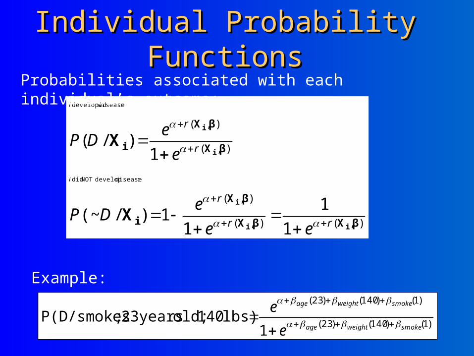
1

1

11)/(~

1)/(

:disease develop NOT did

:disease developed

βXβX

βX

i

βX

βX

i

ii

i

i

i

X

X

rr

r

r

r

ee

eDP

e

eDP

i

i

Probabilities associated with each individual’s outcome:

)1()140()23(

)1()140()23(

1 lbs) 140 old; years 23 ;P(D/smokes

smokeweightage

smokeweightage

e

e

Individual Probability FunctionsIndividual Probability Functions

Example:

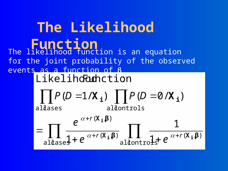
controls all),(

cases all),(

),(

controls allcases all

1

1

1

)/0()/1(

:Function Likelihood

βXβX

βX

ii

ii

i

XX

rr

r

ee

e

DPDP

The Likelihood Function

The likelihood function is an equation for the joint probability of the observed events as a function of

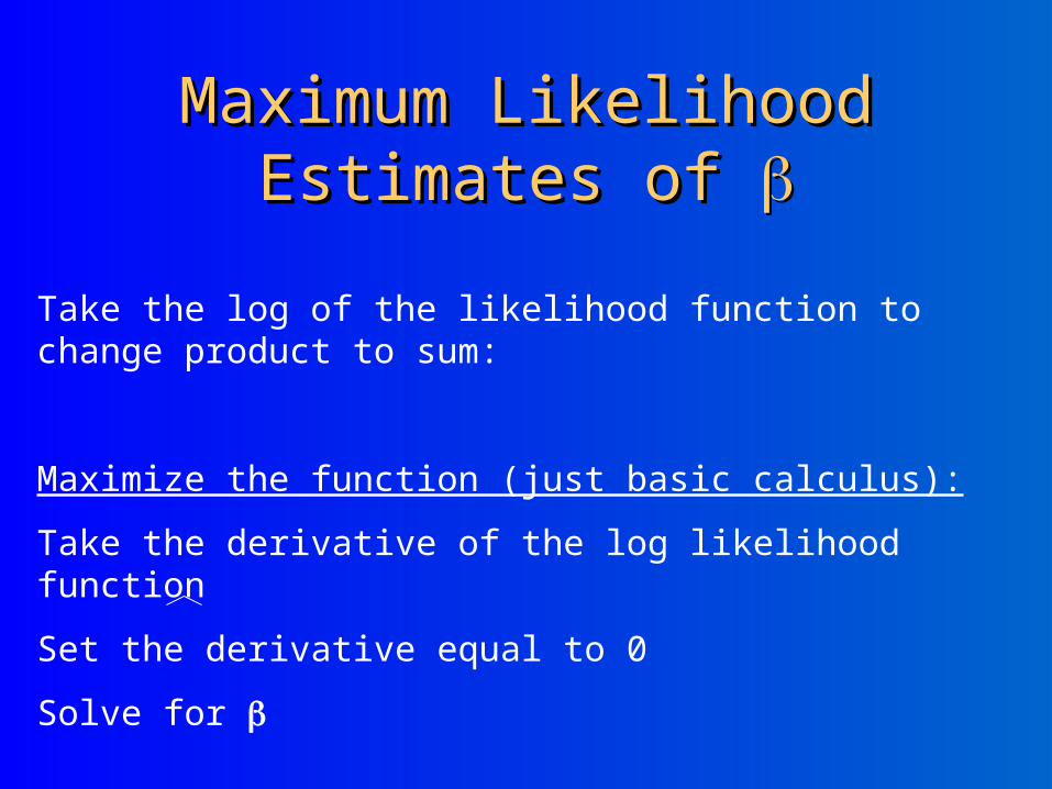
Maximum Likelihood Maximum Likelihood Estimates of Estimates of

Take the log of the likelihood function to change product to sum:

Maximize the function (just basic calculus):

Take the derivative of the log likelihood function

Set the derivative equal to 0

Solve for

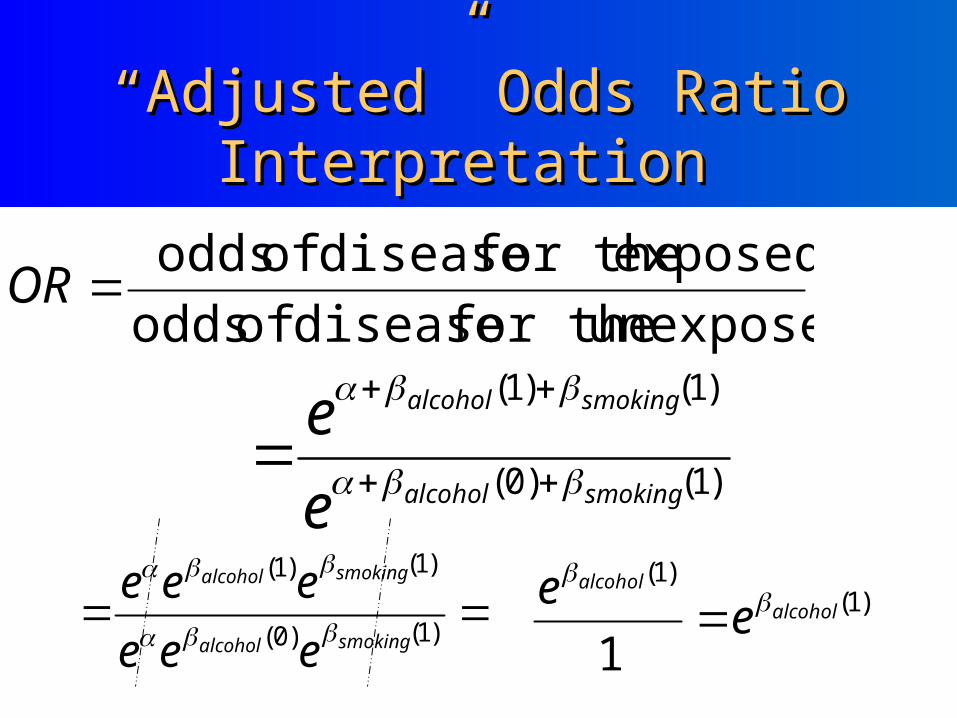
““Adjusted” Odds Ratio Adjusted” Odds Ratio Interpretation Interpretation

unexposed for the disease of odds

exposed for the disease of oddsOR

)1()0(

)1()1(

smokingalcohol

smokingalcohol

e

e

)1()0(

)1()1(

smokingalcohol

smokingalcohol

eee

eee

)1(

)1(

1alcohol

alcohol

ee

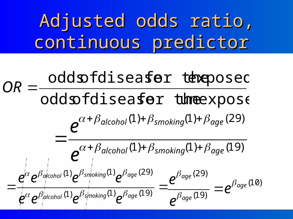
Adjusted odds ratio, Adjusted odds ratio, continuous predictor continuous predictor

unexposed for the disease of odds

exposed for the disease of oddsOR

)19()1()1(

)29()1()1(

agesmokingalcohol

agesmokingalcohol

e

e

)19()1()1(

)29()1()1(

agesmokingalcohol

agesmokingalcohol

eeee

eeee

)10(

)19(

)29(age

age

age

ee

e

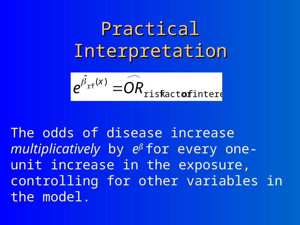
Practical InterpretationPractical Interpretation

interest offactor risk

)(ˆrf ORe

x

The odds of disease increase multiplicatively by eß

for every one-unit increase in the exposure, controlling for other variables in the model.

Simple Logistic RegressionSimple Logistic Regression

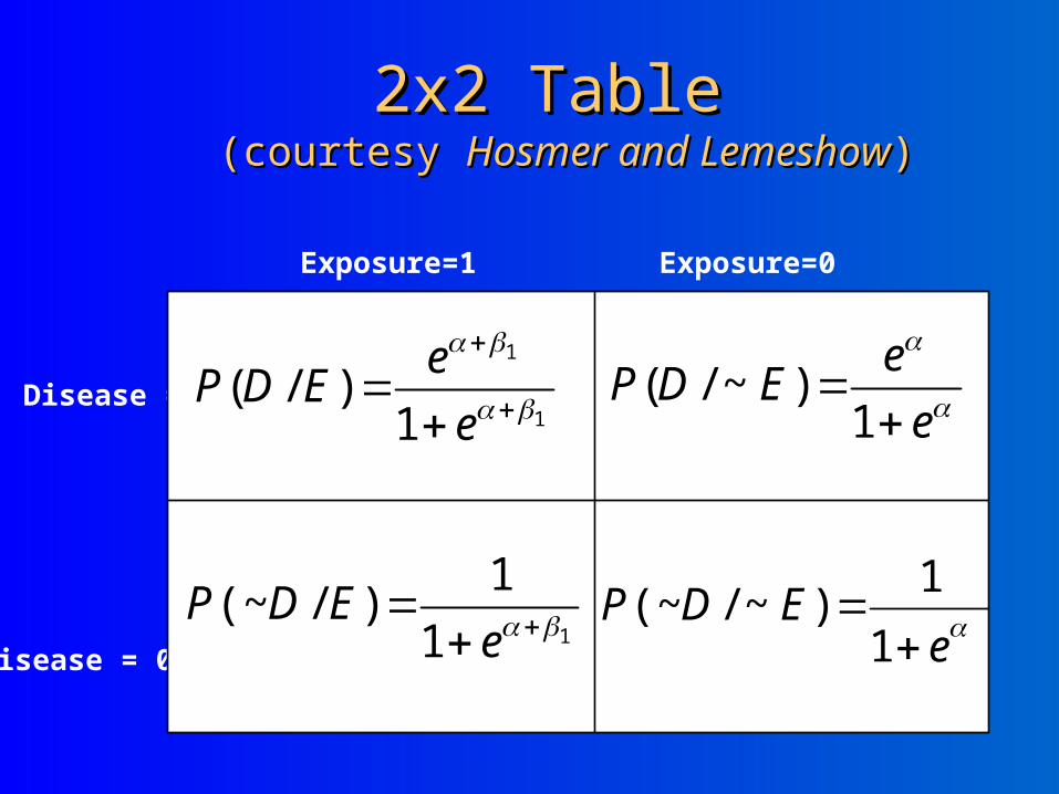
2x2 Table 2x2 Table (courtesy (courtesy Hosmer and LemeshowHosmer and Lemeshow))

 

Exposure=1 Exposure=0

 Disease = 1

Disease = 0 

1

1

1)/(

e

eEDP

e

eEDP

1)~/(

11

1)/(~

eEDP

eEDP

1

1)~/(~

e

e

e

ee

e

OR

11

11

1

11

1

1

1

(courtesy (courtesy Hosmer and LemeshowHosmer and Lemeshow))

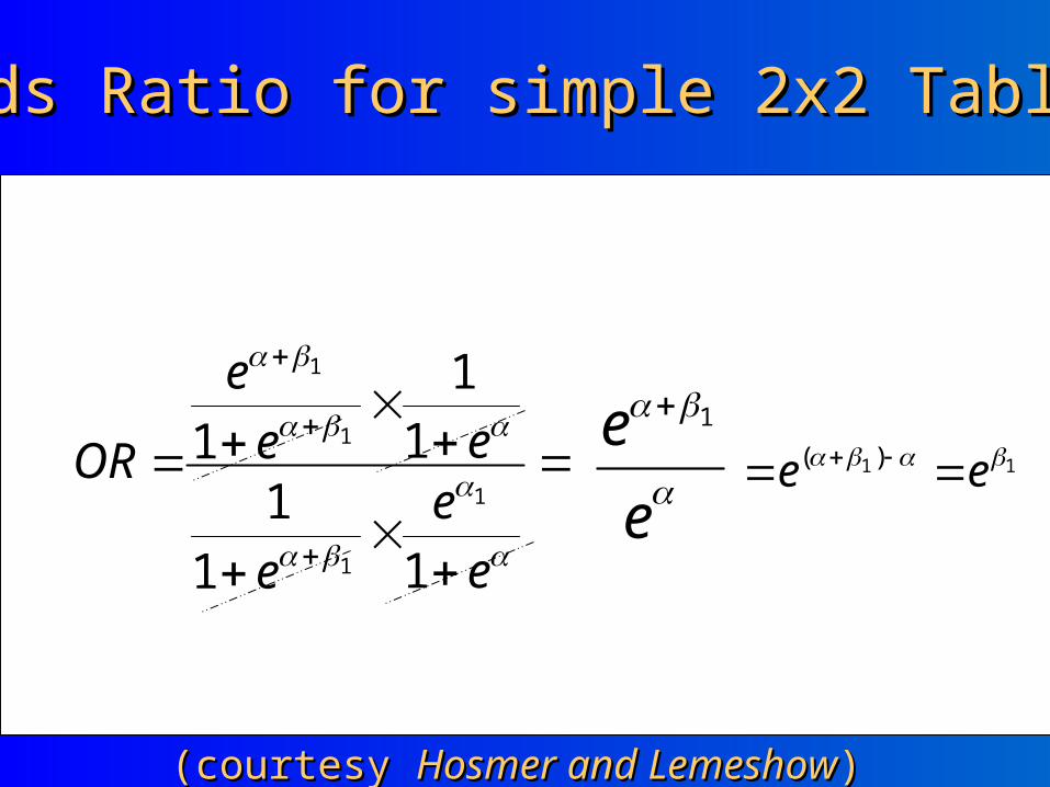
Odds Ratio for simple 2x2 Table Odds Ratio for simple 2x2 Table

e

e 111 )( ee

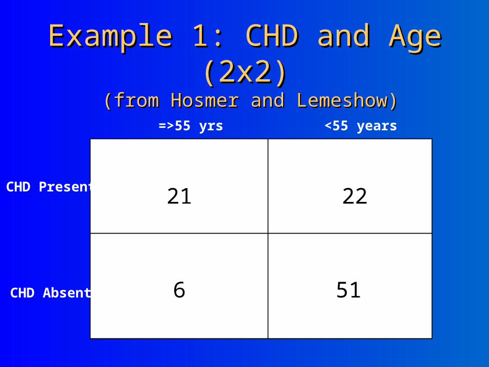
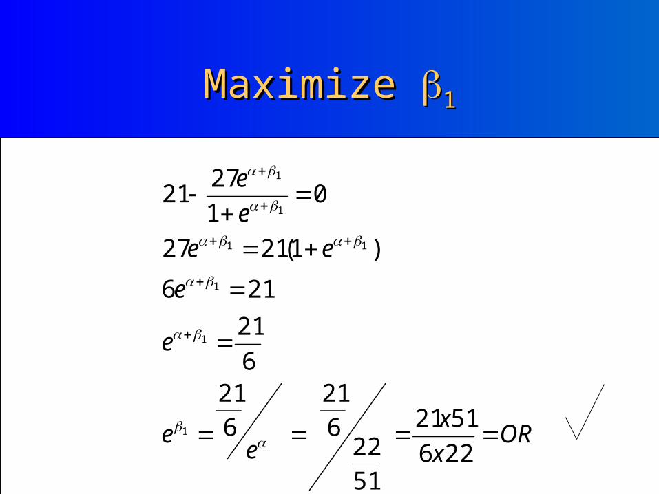
Example 1: CHD and Age Example 1: CHD and Age (2x2)(2x2)

(from Hosmer and Lemeshow) (from Hosmer and Lemeshow)

 

=>55 yrs <55 years

 CHD Present

CHD Absent 

21 22

6 51

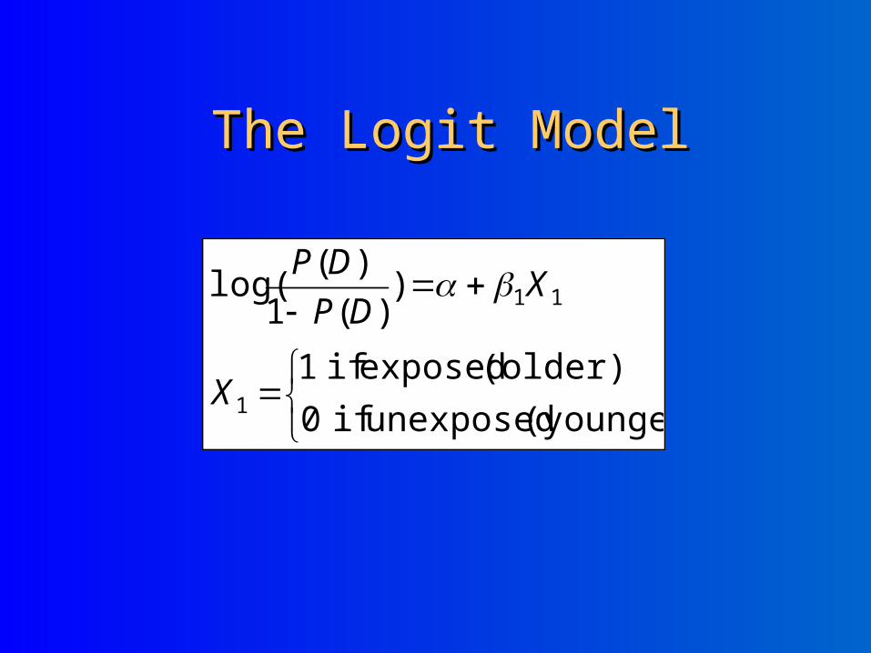
(younger) unexposed if 0

(older) exposed if 1

))(1

)(log(

1

11

X

XDP

DP

The Logit ModelThe Logit Model

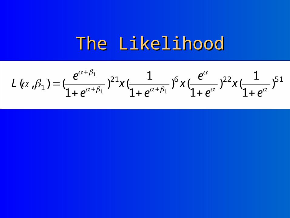
51226211 )

1

1()

1()

1

1()

1(),(

11

1

e

xe

ex

ex

e

eL

The LikelihoodThe Likelihood

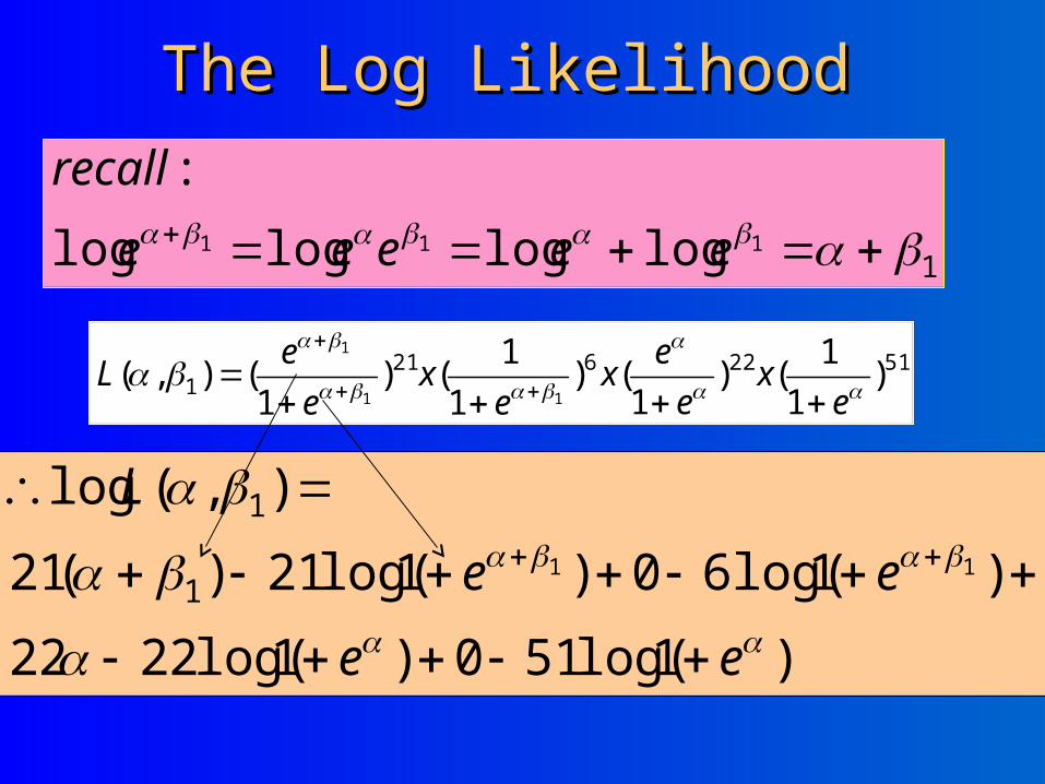
The Log LikelihoodThe Log Likelihood

1111 loglogloglog

:

eeeee

recall

)1log(510)1log(2222

)1log(60)1log(21)(21

),(log

111

1

ee

ee

L

51226211 )

1

1()

1()

1

1()

1(),(

11

1

e

xe

ex

ex

e

eL

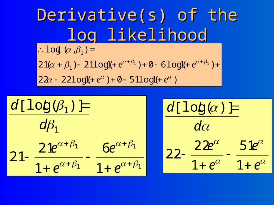
Derivative(s) of the log Derivative(s) of the log likelihoodlikelihood

1

1

1

1

1

6

1

2121

)]([log

1

1

e

e

e

e

d

Ld

e

e

e

e

d

Ld

1

51

1

2222

)]([log

)1log(510)1log(2222

)1log(60)1log(21)(21

),(log

111

1

ee

ee

L

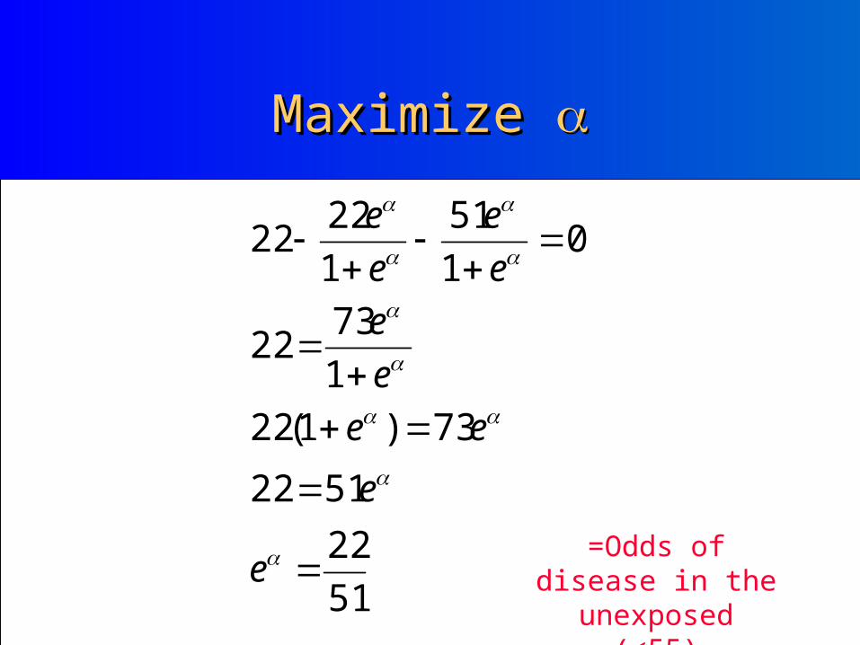
Maximize Maximize

51

22

5122

73)1(22

1

7322

01

51

1

2222

e

e

ee

e

e

e

e

e

e

=Odds of disease in the unexposed (<55)

Maximize Maximize 11

ORx

xe

e

e

e

ee

e

e

226

5121

5122

621

621

6

21

216

)1(2127

01

2721

1

1

1

11

1

1

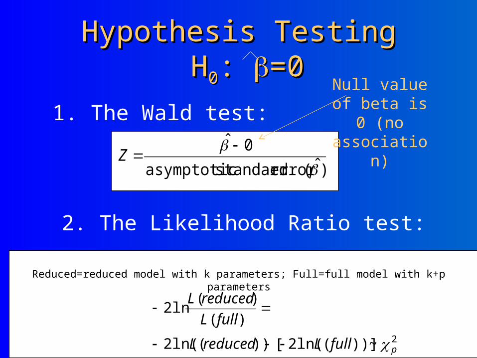
Hypothesis TestingHypothesis Testing H H00: : =0=0

2. The Likelihood Ratio test:

1. The Wald test:

)ˆ(error standard asymptotic

0ˆ

Z

2~))](ln(2[))(ln(2

)(

)(ln2

pfullLreducedL

fullL

reducedL

Reduced=reduced model with k parameters; Full=full model with k+p parameters

Null value of beta is 0 (no association)

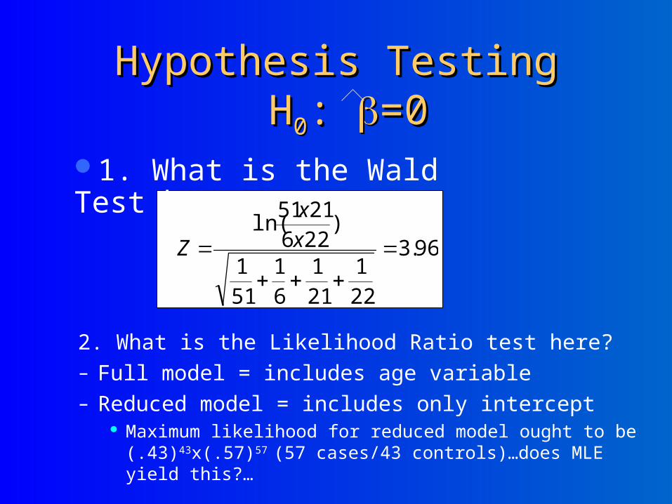
Hypothesis TestingHypothesis Testing H H00: : =0=0

2. What is the Likelihood Ratio test here?– Full model = includes age variable– Reduced model = includes only intercept

Maximum likelihood for reduced model ought to be (.43)43x(.57)57

(57 cases/43 controls)…does MLE yield this?…

96.3

221

211

61

511

)2262151

ln(

x

x

Z

1. What is the Wald Test here?

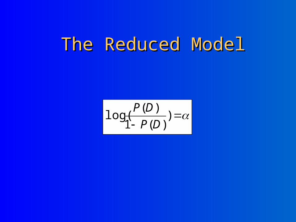
))(1

)(log(

DP

DP

The Reduced ModelThe Reduced Model

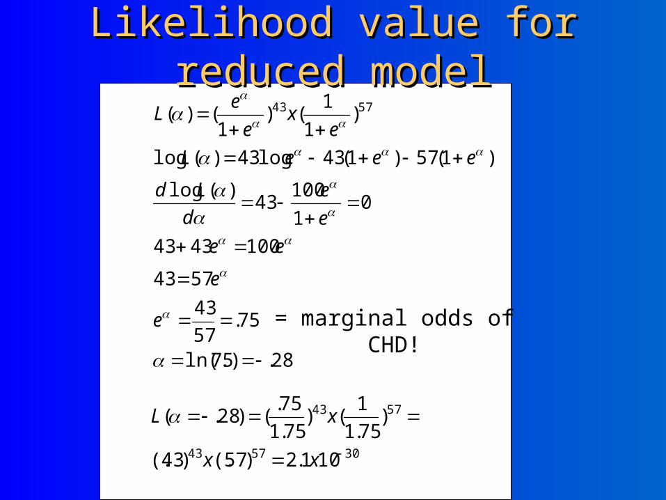
Likelihood value for reduced modelLikelihood value for reduced model

28.)75ln(.

75.57

43

5743

1004343

01

10043

)(log

)1(57)1(43log43)(log

)1

1()

1()( 5743

e

e

ee

e

e

d

Ld

eeeL

ex

e

eL

= marginal odds of CHD!

305743

5743

101.2)57(.)43(.

)75.1

1()

75.1

75.()28.(

xx

xL

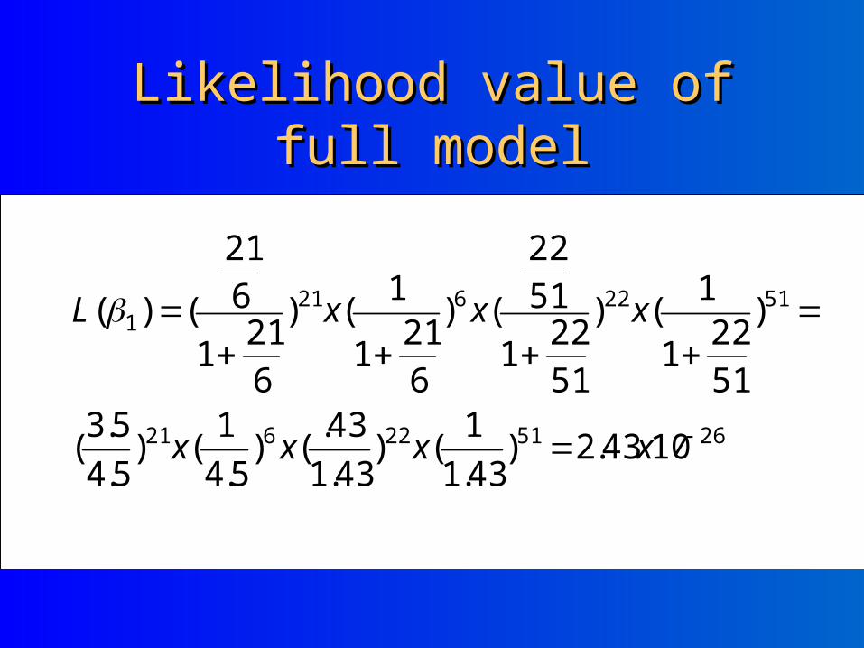
Likelihood value of full modelLikelihood value of full model

265122621

51226211

1043.2)43.1

1()

43.1

43.()

5.4

1()

5.4

5.3(

)

5122

1

1()

5122

1

5122

()

621

1

1()

621

1

621

()(

xxxx

xxxL

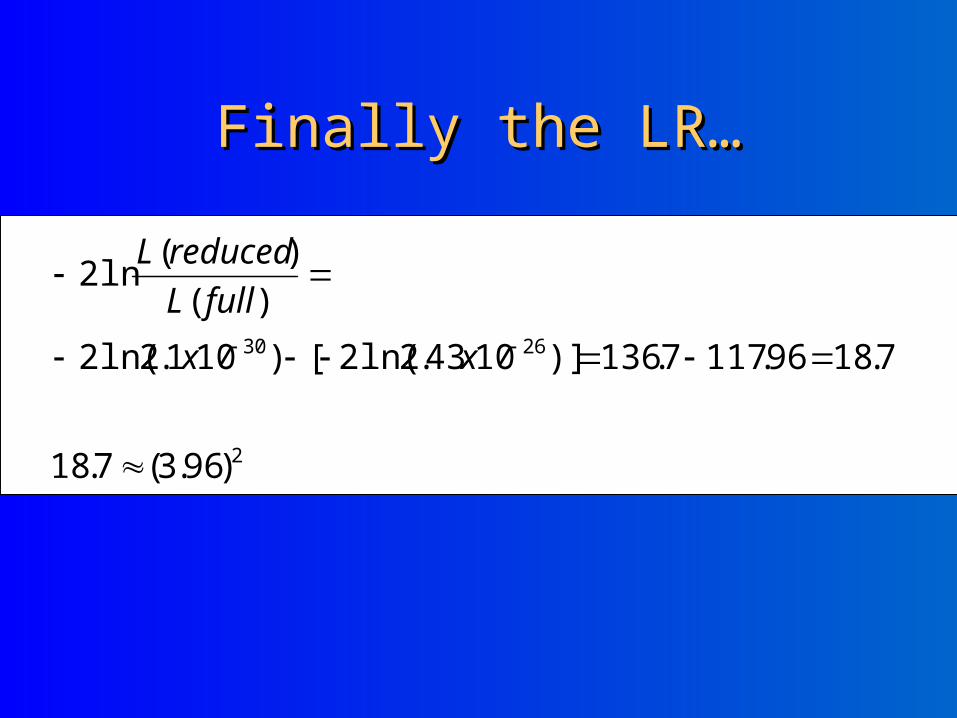
Finally the LR…Finally the LR…

2

2630

)96.3(7.18

7.1896.1177.136)]1043.2ln(2[)101.2ln(2

)(

)(ln2

xx

fullL

reducedL

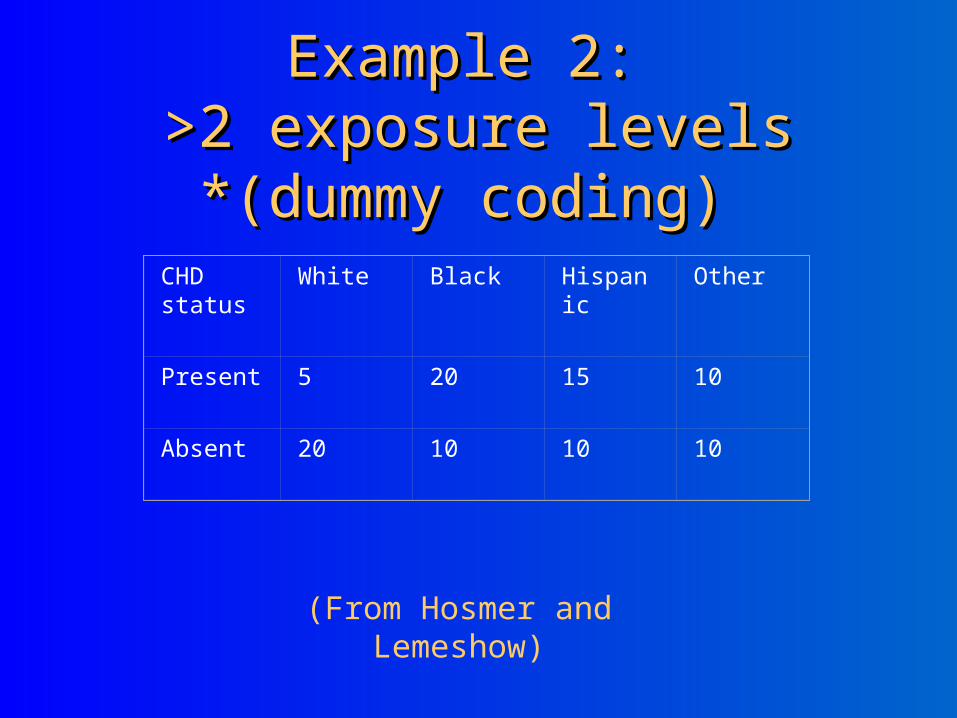
Example 2: Example 2: >2 exposure levels>2 exposure levels*(dummy coding) *(dummy coding)

CHD status

White Black Hispanic Other

Present 5 20 15 10

Absent 20 10 10 10

(From Hosmer and Lemeshow)

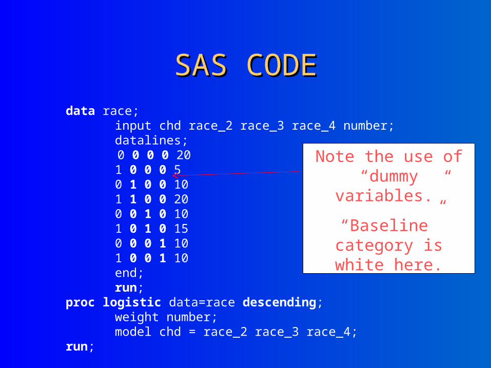
SAS CODESAS CODEdata race;

input chd race_2 race_3 race_4 number;datalines;

0 0 0 0 201 0 0 0 50 1 0 0 101 1 0 0 200 0 1 0 101 0 1 0 150 0 0 1 101 0 0 1 10end;run;

proc logistic data=race descending;weight number;model chd = race_2 race_3 race_4;

run;

Note the use of “dummy variables.”

“Baseline” category is white here.

What’s the likelihood here?What’s the likelihood here?

10101015

1020205

)1

1()

1()

1

1()

1( x

)1

1()

1()

1

1()

1()(

otherwhiteotherwhite

otherwhite

hispwhitehispwhite

hispwhite

blackwhiteblackwhite

blackwhite

whitewhite

white

ex

e

e

ex

e

e

ex

e

ex

ex

e

eL

β

In this case there is more than one unknown beta

(regression coefficient)—so this symbol represents a vector of beta coefficients.

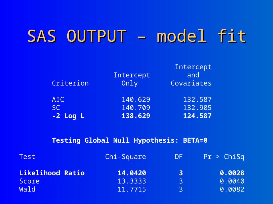
SAS OUTPUT – model fitSAS OUTPUT – model fit 

Intercept Intercept and Criterion Only Covariates  AIC 140.629 132.587 SC 140.709 132.905 -2 Log L 138.629 124.587   Testing Global Null Hypothesis: BETA=0  Test Chi-Square DF Pr > ChiSq  Likelihood Ratio 14.0420 3 0.0028 Score 13.3333 3 0.0040 Wald 11.7715 3 0.0082

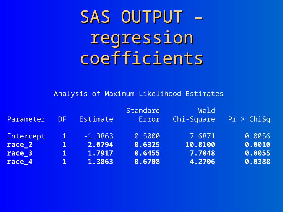
SAS OUTPUT – regression SAS OUTPUT – regression coefficientscoefficients

Analysis of Maximum Likelihood Estimates  Standard Wald Parameter DF Estimate Error Chi-Square Pr > ChiSq  Intercept 1 -1.3863 0.5000 7.6871 0.0056 race_2 1 2.0794 0.6325 10.8100 0.0010 race_3 1 1.7917 0.6455 7.7048 0.0055 race_4 1 1.3863 0.6708 4.2706 0.0388

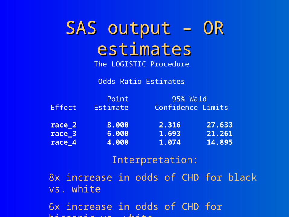
SAS output – OR estimatesSAS output – OR estimates The LOGISTIC Procedure  Odds Ratio Estimates  Point 95% Wald Effect Estimate Confidence Limits  race_2 8.000 2.316 27.633 race_3 6.000 1.693 21.261 race_4 4.000 1.074 14.895

Interpretation:

8x increase in odds of CHD for black vs. white

6x increase in odds of CHD for hispanic vs. white

4x increase in odds of CHD for other vs. white

Example 3: Prostrate Cancer Study Example 3: Prostrate Cancer Study (same data as from lab 3)(same data as from lab 3)

Question: Does PSA level predict tumor penetration into the prostatic capsule (yes/no)? (this is a bad outcome, meaning tumor has spread).

Is this association confounded by race?

Does race modify this association (interaction)?

1.1. What’s the relationship What’s the relationship between PSA (continuous between PSA (continuous variable) and capsule variable) and capsule penetration (binary)?penetration (binary)?

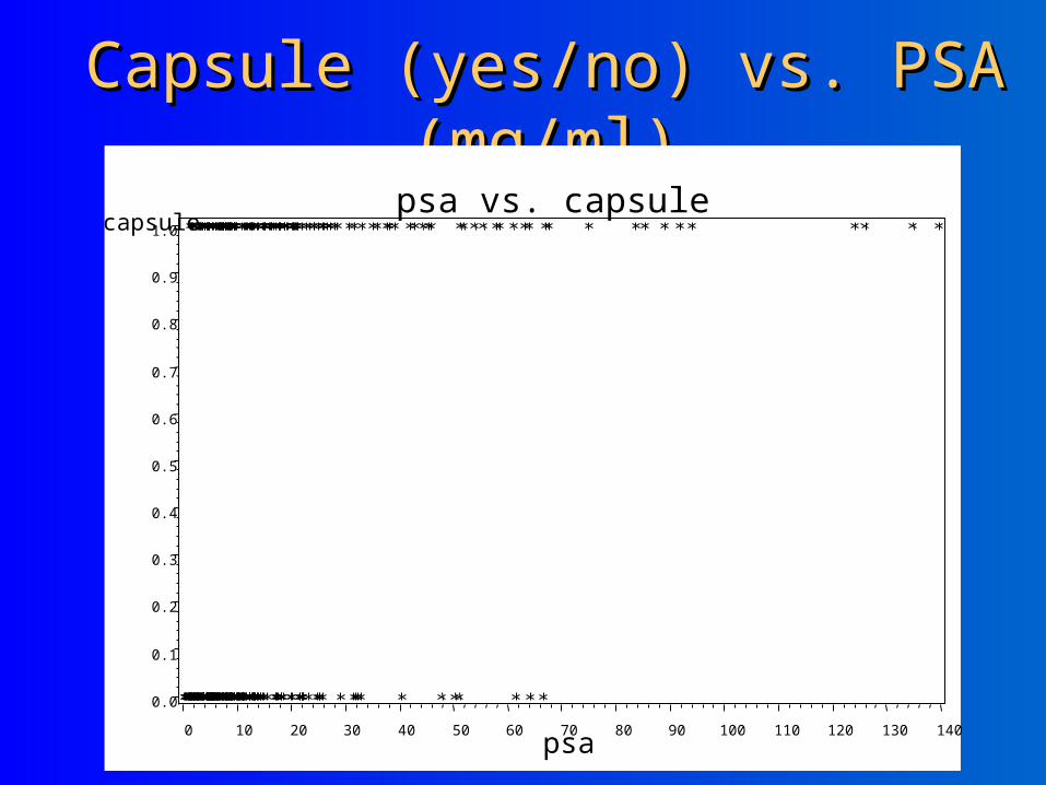
Capsule (yes/no) vs. PSA (mg/ml)Capsule (yes/no) vs. PSA (mg/ml)psa vs. capsule

capsule

0.0

0.1

0.2

0.3

0.4

0.5

0.6

0.7

0.8

0.9

1.0

psa0 10 20 30 40 50 60 70 80 90 100 110 120 130 140

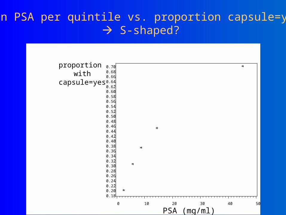
Mean PSA per quintile vs. proportion capsule=yes S-shaped?

proportion with

capsule=yes

0.180.200.220.240.260.280.300.320.340.360.380.400.420.440.460.480.500.520.540.560.580.600.620.640.660.680.70

PSA (mg/ml)0 10 20 30 40 50

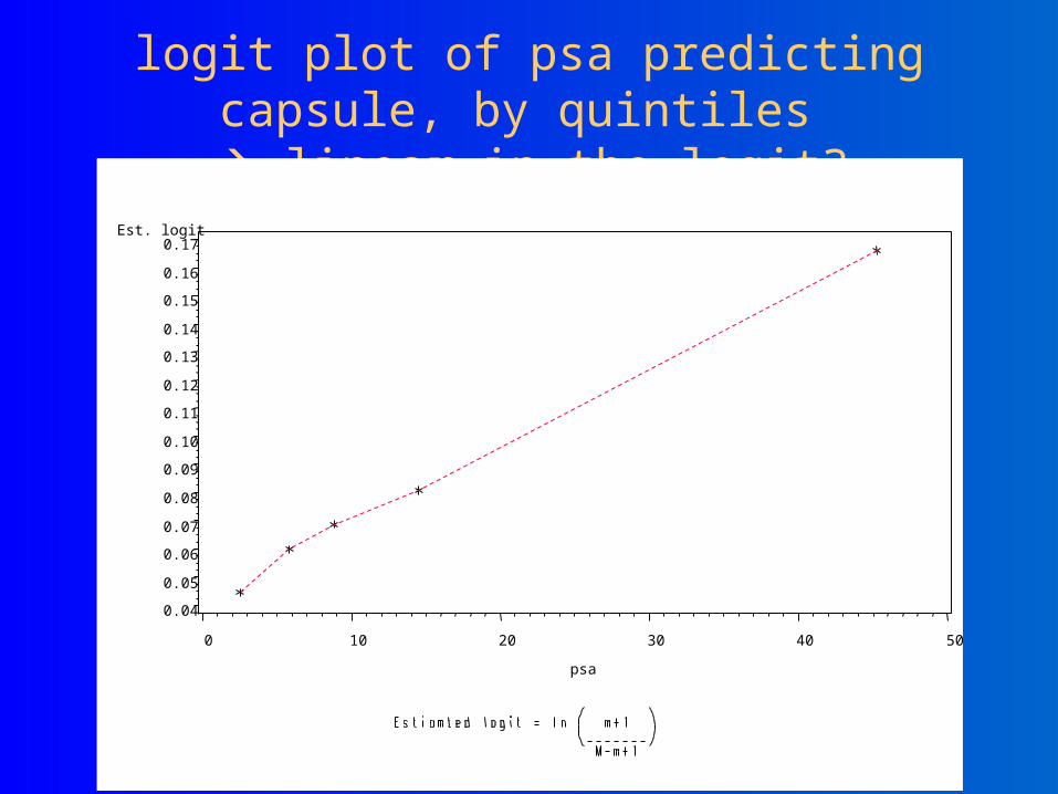
logit plot of psa predicting capsule, by quintiles

linear in the logit?Est. logit

0.04

0.05

0.06

0.07

0.08

0.09

0.10

0.11

0.12

0.13

0.14

0.15

0.16

0.17

psa

0 10 20 30 40 50

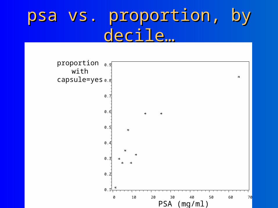
psa vs. proportion, by decile…psa vs. proportion, by decile…

0.1

0.2

0.3

0.4

0.5

0.6

0.7

0.8

0.9

0 10 20 30 40 50 60 70

proportion with

capsule=yes

PSA (mg/ml)

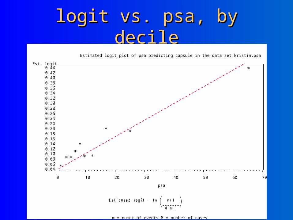
logit vs. psa, by decilelogit vs. psa, by decileEstimated logit plot of psa predicting capsule in the data set kristin.psa

m = numer of events M = number of cases

Est. logit

0.040.060.080.100.120.140.160.180.200.220.240.260.280.300.320.340.360.380.400.420.44

psa

0 10 20 30 40 50 60 70

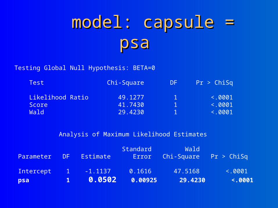
model: capsule = psamodel: capsule = psa  

Testing Global Null Hypothesis: BETA=0  Test Chi-Square DF Pr > ChiSq  Likelihood Ratio 49.1277 1 <.0001 Score 41.7430 1 <.0001 Wald 29.4230 1 <.0001   Analysis of Maximum Likelihood Estimates  Standard Wald Parameter DF Estimate Error Chi-Square Pr > ChiSq  Intercept 1 -1.1137 0.1616 47.5168 <.0001 psa 1 0.0502 0.00925 29.4230 <.0001

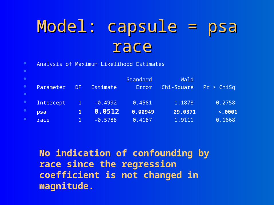
Model: capsule = psa raceModel: capsule = psa race Analysis of Maximum Likelihood Estimates   Standard Wald Parameter DF Estimate Error Chi-Square Pr > ChiSq   Intercept 1 -0.4992 0.4581 1.1878 0.2758 psa 1 0.0512 0.00949 29.0371 <.0001 race 1 -0.5788 0.4187 1.9111 0.1668

No indication of confounding by race since the regression coefficient is not changed in magnitude.

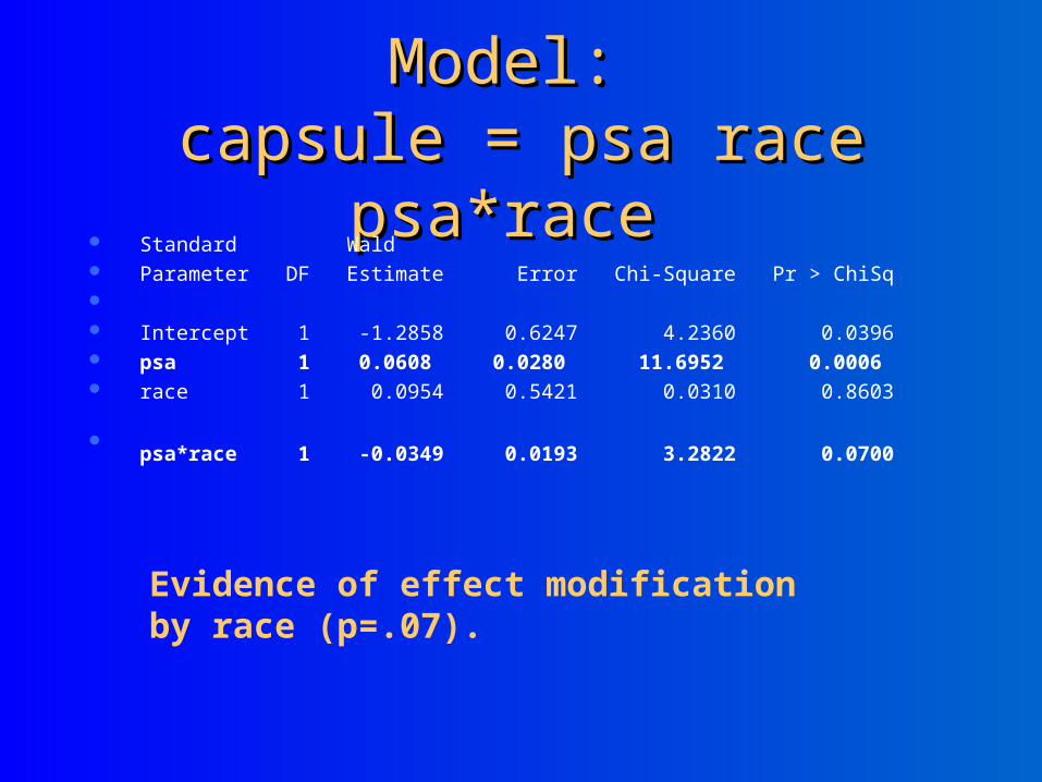
Model: Model: capsule = psa race psa*racecapsule = psa race psa*race

Standard Wald Parameter DF Estimate Error Chi-Square Pr > ChiSq   Intercept 1 -1.2858 0.6247 4.2360 0.0396 psa 1 0.0608 0.0280 11.6952 0.0006 race 1 0.0954 0.5421 0.0310 0.8603

psa*race 1 -0.0349 0.0193 3.2822 0.0700

Evidence of effect modification by race (p=.07).

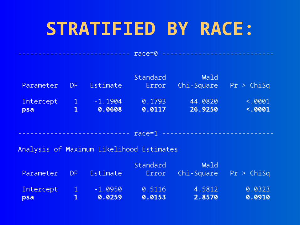
---------------------------- race=0 ---------------------------- 

Standard Wald Parameter DF Estimate Error Chi-Square Pr > ChiSq  Intercept 1 -1.1904 0.1793 44.0820 <.0001 psa 1 0.0608 0.0117 26.9250 <.0001  ---------------------------- race=1 ---------------------------- Analysis of Maximum Likelihood Estimates  Standard Wald Parameter DF Estimate Error Chi-Square Pr > ChiSq  Intercept 1 -1.0950 0.5116 4.5812 0.0323 psa 1 0.0259 0.0153 2.8570 0.0910

STRATIFIED BY RACE:

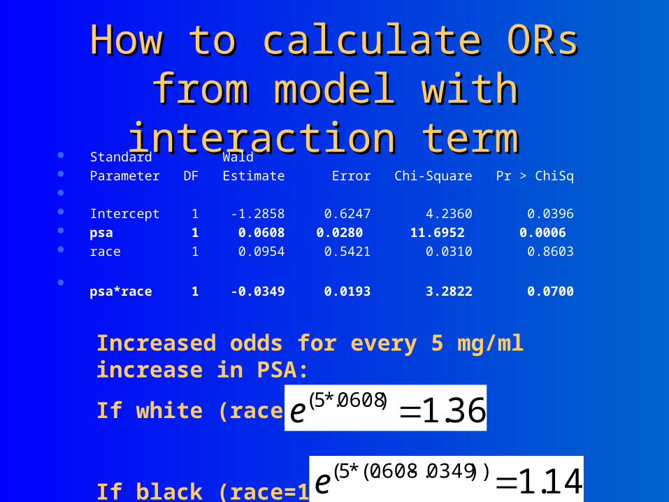
How to calculate ORs from How to calculate ORs from model with interaction termmodel with interaction term

Standard Wald Parameter DF Estimate Error Chi-Square Pr > ChiSq   Intercept 1 -1.2858 0.6247 4.2360 0.0396 psa 1 0.0608 0.0280 11.6952 0.0006 race 1 0.0954 0.5421 0.0310 0.8603

psa*race 1 -0.0349 0.0193 3.2822 0.0700

Increased odds for every 5 mg/ml increase in PSA:

If white (race=0):

If black (race=1):

36.1)0608.*5( e

14.1))0349.0608*(.5( e