long and winding central paths - journée de rentrée du cmap
TRANSCRIPT

Introduction The tropical analogue of linear programming Tropicalizing the central path Tropical lower bound on the complexity of IPMs Conclusion
Long and winding central pathsJournée de rentrée du CMAP
Xavier Allamigeon1 Pascal Benchimol2 Stéphane Gaubert1Michael Joswig3
1INRIA Saclay – Ile-de-France and CMAP, Ecole Polytechnique, CNRS2EDF Lab
3Institut für Mathematik, Technische Universität Berlin
October 3rd, 2018
Long and winding central paths | Allamigeon, Benchimol, Gaubert, Joswig | 1/37

Introduction The tropical analogue of linear programming Tropicalizing the central path Tropical lower bound on the complexity of IPMs Conclusion
Motivation: the complexity of linear programming
DefinitionA linear program is an optimization problem of the form:
minimize c⊤xsubject to Ax ⩽ b, x ∈ Rn
where A ∈ Rm×n, b ∈ Rm, c ∈ Rn.
minimize x+ 3ysubject to x+ y ⩾ 3
23 ⩾ x+ 3y4x ⩾ 1+ y
11+ y ⩾ 2x2y ⩾ 2
Long and winding central paths | Allamigeon, Benchimol, Gaubert, Joswig | 2/37

Introduction The tropical analogue of linear programming Tropicalizing the central path Tropical lower bound on the complexity of IPMs Conclusion
Motivation: the complexity of linear programming (2)
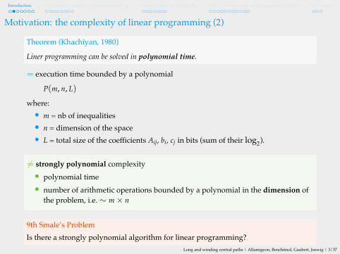
Theorem (Khachiyan, 1980)Liner programming can be solved in polynomial time.
= execution time bounded by a polynomialP(m, n, L)
where:• m = nb of inequalities• n = dimension of the space• L = total size of the coefficients Aij, bi, cj in bits (sum of their log2).
= strongly polynomial complexity• polynomial time• number of arithmetic operations bounded by a polynomial in the dimension ofthe problem, i.e.∼ m× n
9th Smale’s ProblemIs there a strongly polynomial algorithm for linear programming?
Long and winding central paths | Allamigeon, Benchimol, Gaubert, Joswig | 3/37

Introduction The tropical analogue of linear programming Tropicalizing the central path Tropical lower bound on the complexity of IPMs Conclusion
Motivation: the complexity of linear programming (2)
Theorem (Khachiyan, 1980)Liner programming can be solved in polynomial time.
= execution time bounded by a polynomialP(m, n, L)
where:• m = nb of inequalities• n = dimension of the space• L = total size of the coefficients Aij, bi, cj in bits (sum of their log2).
= strongly polynomial complexity• polynomial time• number of arithmetic operations bounded by a polynomial in the dimension ofthe problem, i.e.∼ m× n
9th Smale’s ProblemIs there a strongly polynomial algorithm for linear programming?
Long and winding central paths | Allamigeon, Benchimol, Gaubert, Joswig | 3/37

Introduction The tropical analogue of linear programming Tropicalizing the central path Tropical lower bound on the complexity of IPMs Conclusion
Motivation: the complexity of linear programming (3)
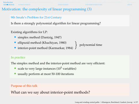
9th Smale’s Problem for 21st CenturyIs there a strongly polynomial algorithm for linear programming?
Existing algorithms for LP:• simplex method (Dantzig, 1947)• ellipsoid method (Khachiyan, 1980)• interior-point method (Karmarkar, 1984)
In practiceThe simplex method and the interior-point method are very efficient:• scale to very large instances (105 variables)• usually perform at most 50-100 iterations
Purpose of this talk
What can we say about interior-point methods?
Long and winding central paths | Allamigeon, Benchimol, Gaubert, Joswig | 4/37

Introduction The tropical analogue of linear programming Tropicalizing the central path Tropical lower bound on the complexity of IPMs Conclusion
Motivation: the complexity of linear programming (3)
9th Smale’s Problem for 21st CenturyIs there a strongly polynomial algorithm for linear programming?
Existing algorithms for LP:• simplex method (Dantzig, 1947)• ellipsoid method (Khachiyan, 1980)• interior-point method (Karmarkar, 1984)
In practiceThe simplex method and the interior-point method are very efficient:• scale to very large instances (105 variables)• usually perform at most 50-100 iterations
Purpose of this talk
What can we say about interior-point methods?
polynomial time
Long and winding central paths | Allamigeon, Benchimol, Gaubert, Joswig | 4/37

Introduction The tropical analogue of linear programming Tropicalizing the central path Tropical lower bound on the complexity of IPMs Conclusion
Log-barrier interior point methods for linear programming
Consider the following LP
minimize c⊤xsubject to Ax ⩽ b , x ∈ Rn (P)
Logarithmic barrier penalization
minimize c⊤x− µm∑i=1
log(bi − Aix)
subject to Aix < bi , i = 1, . . . ,m(Pµ)
where µ > 0.
For all µ > 0, Problem (Pµ) has a unique optimal solution xµ.Moreover, xµ converges to an optimal solution of (P) when µ → 0+.
DefinitionThe central path is the curve µ 7→ xµ.
Principle of log-barrier IPMFollow the central path with µ 0 up tothe solution of (P)
approximately
.
• stay in a certain “neighborhood” ofthe central path
• use Newton descent directions toiterate
• different choices of steps (short, long,predictor/corrector, etc)
Long and winding central paths | Allamigeon, Benchimol, Gaubert, Joswig | 5/37

Introduction The tropical analogue of linear programming Tropicalizing the central path Tropical lower bound on the complexity of IPMs Conclusion
Log-barrier interior point methods for linear programming
Consider the following LP
minimize c⊤xsubject to Ax ⩽ b , x ∈ Rn (P)
Logarithmic barrier penalization
minimize c⊤x− µm∑i=1
log(bi − Aix)
subject to Aix < bi , i = 1, . . . ,m(Pµ)
where µ > 0.For all µ > 0, Problem (Pµ) has a unique optimal solution xµ.Moreover, xµ converges to an optimal solution of (P) when µ → 0+.
DefinitionThe central path is the curve µ 7→ xµ.
Principle of log-barrier IPMFollow the central path with µ 0 up tothe solution of (P)
approximately
.
• stay in a certain “neighborhood” ofthe central path
• use Newton descent directions toiterate
• different choices of steps (short, long,predictor/corrector, etc)
Long and winding central paths | Allamigeon, Benchimol, Gaubert, Joswig | 5/37

Introduction The tropical analogue of linear programming Tropicalizing the central path Tropical lower bound on the complexity of IPMs Conclusion
Log-barrier interior point methods for linear programming
Consider the following LP
minimize c⊤xsubject to Ax ⩽ b , x ∈ Rn (P)
Logarithmic barrier penalization
minimize c⊤x− µm∑i=1
log(bi − Aix)
subject to Aix < bi , i = 1, . . . ,m(Pµ)
where µ > 0.
For all µ > 0, Problem (Pµ) has a unique optimal solution xµ.Moreover, xµ converges to an optimal solution of (P) when µ → 0+.
DefinitionThe central path is the curve µ 7→ xµ.
Principle of log-barrier IPMFollow the central path with µ 0 up tothe solution of (P)
approximately
.
• stay in a certain “neighborhood” ofthe central path
• use Newton descent directions toiterate
• different choices of steps (short, long,predictor/corrector, etc)
Long and winding central paths | Allamigeon, Benchimol, Gaubert, Joswig | 5/37

Introduction The tropical analogue of linear programming Tropicalizing the central path Tropical lower bound on the complexity of IPMs Conclusion
Log-barrier interior point methods for linear programming
Consider the following LP
minimize c⊤xsubject to Ax ⩽ b , x ∈ Rn (P)
Logarithmic barrier penalization
minimize c⊤x− µm∑i=1
log(bi − Aix)
subject to Aix < bi , i = 1, . . . ,m(Pµ)
where µ > 0.
For all µ > 0, Problem (Pµ) has a unique optimal solution xµ.Moreover, xµ converges to an optimal solution of (P) when µ → 0+.
DefinitionThe central path is the curve µ 7→ xµ.
Principle of log-barrier IPMFollow the central path with µ 0 up tothe solution of (P) approximately.
• stay in a certain “neighborhood” ofthe central path
• use Newton descent directions toiterate
• different choices of steps (short, long,predictor/corrector, etc)
Long and winding central paths | Allamigeon, Benchimol, Gaubert, Joswig | 5/37
Introduction The tropical analogue of linear programming Tropicalizing the central path Tropical lower bound on the complexity of IPMs Conclusion
The curvature of the central path
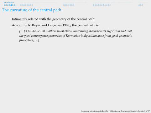
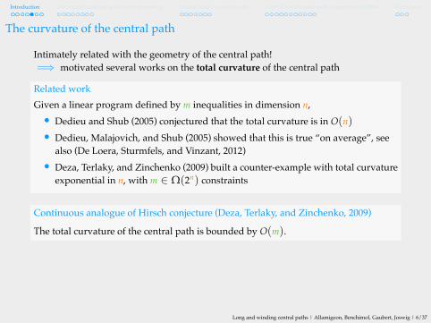
Intimately related with the geometry of the central path!According to Bayer and Lagarias (1989), the central path is
[…] a fundamental mathematical object underlying Karmarkar’s algorithm and thatthe good convergence properties of Karmarkar’s algorithm arise from good geometricproperties […]
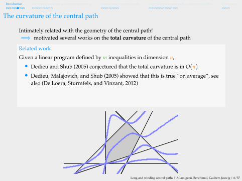
=⇒ motivated several works on the total curvature of the central path
Related workGiven a linear program defined by m inequalities in dimension n,• Dedieu and Shub (2005) conjectured that the total curvature is in O(n)
• Dedieu, Malajovich, and Shub (2005) showed that this is true “on average”, seealso (De Loera, Sturmfels, and Vinzant, 2012)
• Deza, Terlaky, and Zinchenko (2009) built a counter-example with total curvatureexponential in n, with m ∈ Ω(2n) constraints
Continuous analogue of Hirsch conjecture (Deza, Terlaky, and Zinchenko, 2009)The total curvature of the central path is bounded by O(m).
ObstacleThere is no explicit relation between the curvature of the central path and thecomplexity of interior point methods.
Long and winding central paths | Allamigeon, Benchimol, Gaubert, Joswig | 6/37

Introduction The tropical analogue of linear programming Tropicalizing the central path Tropical lower bound on the complexity of IPMs Conclusion
The curvature of the central path
Intimately related with the geometry of the central path!=⇒ motivated several works on the total curvature of the central path
Related workGiven a linear program defined by m inequalities in dimension n,• Dedieu and Shub (2005) conjectured that the total curvature is in O(n)
• Dedieu, Malajovich, and Shub (2005) showed that this is true “on average”, seealso (De Loera, Sturmfels, and Vinzant, 2012)
• Deza, Terlaky, and Zinchenko (2009) built a counter-example with total curvatureexponential in n, with m ∈ Ω(2n) constraints
Continuous analogue of Hirsch conjecture (Deza, Terlaky, and Zinchenko, 2009)The total curvature of the central path is bounded by O(m).
ObstacleThere is no explicit relation between the curvature of the central path and thecomplexity of interior point methods.
Long and winding central paths | Allamigeon, Benchimol, Gaubert, Joswig | 6/37
Introduction The tropical analogue of linear programming Tropicalizing the central path Tropical lower bound on the complexity of IPMs Conclusion
The curvature of the central path
Intimately related with the geometry of the central path!=⇒ motivated several works on the total curvature of the central pathRelated workGiven a linear program defined by m inequalities in dimension n,• Dedieu and Shub (2005) conjectured that the total curvature is in O(n)• Dedieu, Malajovich, and Shub (2005) showed that this is true “on average”, seealso (De Loera, Sturmfels, and Vinzant, 2012)
• Deza, Terlaky, and Zinchenko (2009) built a counter-example with total curvatureexponential in n, with m ∈ Ω(2n) constraints
Continuous analogue of Hirsch conjecture (Deza, Terlaky, and Zinchenko, 2009)The total curvature of the central path is bounded by O(m).
ObstacleThere is no explicit relation between the curvature of the central path and thecomplexity of interior point methods.
Long and winding central paths | Allamigeon, Benchimol, Gaubert, Joswig | 6/37

Introduction The tropical analogue of linear programming Tropicalizing the central path Tropical lower bound on the complexity of IPMs Conclusion
The curvature of the central path
Intimately related with the geometry of the central path!=⇒ motivated several works on the total curvature of the central path
Related workGiven a linear program defined by m inequalities in dimension n,• Dedieu and Shub (2005) conjectured that the total curvature is in O(n)• Dedieu, Malajovich, and Shub (2005) showed that this is true “on average”, seealso (De Loera, Sturmfels, and Vinzant, 2012)
• Deza, Terlaky, and Zinchenko (2009) built a counter-example with total curvatureexponential in n, with m ∈ Ω(2n) constraints
Continuous analogue of Hirsch conjecture (Deza, Terlaky, and Zinchenko, 2009)The total curvature of the central path is bounded by O(m).
ObstacleThere is no explicit relation between the curvature of the central path and thecomplexity of interior point methods.
Long and winding central paths | Allamigeon, Benchimol, Gaubert, Joswig | 6/37

Introduction The tropical analogue of linear programming Tropicalizing the central path Tropical lower bound on the complexity of IPMs Conclusion
This talk
Main resultLog-barrier interior point methods are not strongly polynomial.
Consider the following parametric family of LPs:minimize x1subject to x1 ⩽ t2
x2 ⩽ tx2j+1 ⩽ t x2j−1 , x2j+1 ⩽ t x2jx2j+2 ⩽ t1−1/2j (x2j−1 + x2j)x2r−1 ⩾ 0 , x2r ⩾ 0
1 ⩽ j < rLWr(t)
CorollaryThe number of iterations of any log-barrier interior point algorithm is exponential in r on thelinear program LWr(t), provided that t > 1 is sufficiently large.
RemarkThe total curvature of the central path of LWr(t) is also exponential.
Long and winding central paths | Allamigeon, Benchimol, Gaubert, Joswig | 7/37

Introduction The tropical analogue of linear programming Tropicalizing the central path Tropical lower bound on the complexity of IPMs Conclusion
Outline of the talk
Key ingredientWe set up a tropical lower bound on the iteration complexity of log-barrier IPM.
1 The tropical analogue of linear programming
2 Tropicalizing the central path
3 Tropical lower bound on the complexity of IPMs
4 Conclusion
Long and winding central paths | Allamigeon, Benchimol, Gaubert, Joswig | 8/37

Introduction The tropical analogue of linear programming Tropicalizing the central path Tropical lower bound on the complexity of IPMs Conclusion
Outline of the talk
1 The tropical analogue of linear programming
2 Tropicalizing the central path
3 Tropical lower bound on the complexity of IPMs
4 Conclusion
Long and winding central paths | Allamigeon, Benchimol, Gaubert, Joswig | 9/37

Introduction The tropical analogue of linear programming Tropicalizing the central path Tropical lower bound on the complexity of IPMs Conclusion
Tropical algebra and tropical polyhedra
Tropical algebra refers to the semiring T := R ∪ −∞ where:• the addition x⊕ y is max(x, y)• the multiplication x⊙ y is x+ y
Tropical operations extend to matrices and vectors:
A⊕ B = (Aij ⊕ Bij)ij A⊙ B =(⊕
kAik ⊙ Bkj
)ij
Long and winding central paths | Allamigeon, Benchimol, Gaubert, Joswig | 10/37

Introduction The tropical analogue of linear programming Tropicalizing the central path Tropical lower bound on the complexity of IPMs Conclusion
Tropical algebra and tropical polyhedra (2)
A tropical polyhedron is the set of solutions x ∈ Tn of a system of the form:
A+ ⊙ x⊕ b+ ⩾ A− ⊙ x⊕ b−
with A+,A− ∈ Tm×n and b+, b− ∈ Tm.
x1
x2
Long and winding central paths | Allamigeon, Benchimol, Gaubert, Joswig | 11/37

Introduction The tropical analogue of linear programming Tropicalizing the central path Tropical lower bound on the complexity of IPMs Conclusion
Tropical algebra and tropical polyhedra (2)
A tropical polyhedron is the set of solutions x ∈ Tn of a system of the form:
A+ ⊙ x⊕ b+ ⩾ A− ⊙ x⊕ b−
with A+,A− ∈ Tm×n and b+, b− ∈ Tm.
x1
x2
( 0 1−∞ 0−∞ 0−∞ −∞4 −∞
)⊙(x1x2
)⊕(−∞
−∞48
−∞
)
⩾( −∞ −∞
−10 −∞−3 −∞0 2
−∞ 0
)⊙(x1x2
)⊕( 3
1−∞−∞5
)
Long and winding central paths | Allamigeon, Benchimol, Gaubert, Joswig | 11/37

Introduction The tropical analogue of linear programming Tropicalizing the central path Tropical lower bound on the complexity of IPMs Conclusion
Tropical algebra and tropical polyhedra (2)
A tropical polyhedron is the set of solutions x ∈ Tn of a system of the form:
A+ ⊙ x⊕ b+ ⩾ A− ⊙ x⊕ b−
with A+,A− ∈ Tm×n and b+, b− ∈ Tm.
x1
x2
max(x1, 1+ x2) ⩾ 3x2 ⩾ max(−10+ x1, 1)
max(x2, 4) ⩾ −3+ x18 ⩾ max(x1, 2+ x2)
4+ x1 ⩾ max(x2, 5)
Long and winding central paths | Allamigeon, Benchimol, Gaubert, Joswig | 11/37

Introduction The tropical analogue of linear programming Tropicalizing the central path Tropical lower bound on the complexity of IPMs Conclusion
Tropical polyhedra vs convex polyhedra
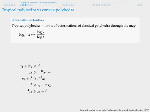
Alternative definitionTropical polyhedra= limits of deformations of classical polyhedra through the map
logt : x 7→ log xlog t
Maslov dequantization
max(logt x, logt y) ⩽ logt(x+ y) ⩽ max(logt x, logt y) + logt 2
logt(x · y) = logt x+ logt y
Our goal: tropicalizing the central pathStudy the central path of a parametric family of LPs:
minimize c(t)⊤xsubject to A(t)x ⩽ b(t) , x ⩾ 0
and its deformation by the map logt(·), when t goes to+∞.
Long and winding central paths | Allamigeon, Benchimol, Gaubert, Joswig | 12/37
Introduction The tropical analogue of linear programming Tropicalizing the central path Tropical lower bound on the complexity of IPMs Conclusion
Tropical polyhedra vs convex polyhedra
Alternative definitionTropical polyhedra= limits of deformations of classical polyhedra through the map
logt : x 7→ log xlog t
x1 + tx2 ⩾ t3
x2 ⩾ t−10x1 + tx2 + t4 ⩾ t−3x1
t8 ⩾ x1 + t2x2t4x1 ⩾ x2 + t5
logt x1
logt x2
Maslov dequantization
max(logt x, logt y) ⩽ logt(x+ y) ⩽ max(logt x, logt y) + logt 2
logt(x · y) = logt x+ logt y
Our goal: tropicalizing the central pathStudy the central path of a parametric family of LPs:
minimize c(t)⊤xsubject to A(t)x ⩽ b(t) , x ⩾ 0
and its deformation by the map logt(·), when t goes to+∞.
Long and winding central paths | Allamigeon, Benchimol, Gaubert, Joswig | 12/37

Introduction The tropical analogue of linear programming Tropicalizing the central path Tropical lower bound on the complexity of IPMs Conclusion
Tropical polyhedra vs convex polyhedra
Alternative definitionTropical polyhedra= limits of deformations of classical polyhedra through the map
logt : x 7→ log xlog t
x1 + tx2 ⩾ t3
x2 ⩾ t−10x1 + tx2 + t4 ⩾ t−3x1
t8 ⩾ x1 + t2x2t4x1 ⩾ x2 + t5
logt(·)t = 5
logt x1
logt x2
Maslov dequantization
max(logt x, logt y) ⩽ logt(x+ y) ⩽ max(logt x, logt y) + logt 2
logt(x · y) = logt x+ logt y
Our goal: tropicalizing the central pathStudy the central path of a parametric family of LPs:
minimize c(t)⊤xsubject to A(t)x ⩽ b(t) , x ⩾ 0
and its deformation by the map logt(·), when t goes to+∞.
Long and winding central paths | Allamigeon, Benchimol, Gaubert, Joswig | 12/37

Introduction The tropical analogue of linear programming Tropicalizing the central path Tropical lower bound on the complexity of IPMs Conclusion
Tropical polyhedra vs convex polyhedra
Alternative definitionTropical polyhedra= limits of deformations of classical polyhedra through the map
logt : x 7→ log xlog t
x1 + tx2 ⩾ t3
x2 ⩾ t−10x1 + tx2 + t4 ⩾ t−3x1
t8 ⩾ x1 + t2x2t4x1 ⩾ x2 + t5
logt(·)t = 10
logt x1
logt x2
Maslov dequantization
max(logt x, logt y) ⩽ logt(x+ y) ⩽ max(logt x, logt y) + logt 2
logt(x · y) = logt x+ logt y
Our goal: tropicalizing the central pathStudy the central path of a parametric family of LPs:
minimize c(t)⊤xsubject to A(t)x ⩽ b(t) , x ⩾ 0
and its deformation by the map logt(·), when t goes to+∞.
Long and winding central paths | Allamigeon, Benchimol, Gaubert, Joswig | 12/37

Introduction The tropical analogue of linear programming Tropicalizing the central path Tropical lower bound on the complexity of IPMs Conclusion
Tropical polyhedra vs convex polyhedra
Alternative definitionTropical polyhedra= limits of deformations of classical polyhedra through the map
logt : x 7→ log xlog t
x1 + tx2 ⩾ t3
x2 ⩾ t−10x1 + tx2 + t4 ⩾ t−3x1
t8 ⩾ x1 + t2x2t4x1 ⩾ x2 + t5
logt(·)t = 100
logt x1
logt x2
Maslov dequantization
max(logt x, logt y) ⩽ logt(x+ y) ⩽ max(logt x, logt y) + logt 2
logt(x · y) = logt x+ logt y
Our goal: tropicalizing the central pathStudy the central path of a parametric family of LPs:
minimize c(t)⊤xsubject to A(t)x ⩽ b(t) , x ⩾ 0
and its deformation by the map logt(·), when t goes to+∞.
Long and winding central paths | Allamigeon, Benchimol, Gaubert, Joswig | 12/37

Introduction The tropical analogue of linear programming Tropicalizing the central path Tropical lower bound on the complexity of IPMs Conclusion
Tropical polyhedra vs convex polyhedra
Alternative definitionTropical polyhedra= limits of deformations of classical polyhedra through the map
logt : x 7→ log xlog t
x1 + tx2 ⩾ t3
x2 ⩾ t−10x1 + tx2 + t4 ⩾ t−3x1
t8 ⩾ x1 + t2x2t4x1 ⩾ x2 + t5
logt(·)t = 1000
logt x1
logt x2
Maslov dequantization
max(logt x, logt y) ⩽ logt(x+ y) ⩽ max(logt x, logt y) + logt 2
logt(x · y) = logt x+ logt y
Our goal: tropicalizing the central pathStudy the central path of a parametric family of LPs:
minimize c(t)⊤xsubject to A(t)x ⩽ b(t) , x ⩾ 0
and its deformation by the map logt(·), when t goes to+∞.
Long and winding central paths | Allamigeon, Benchimol, Gaubert, Joswig | 12/37

Introduction The tropical analogue of linear programming Tropicalizing the central path Tropical lower bound on the complexity of IPMs Conclusion
Tropical polyhedra vs convex polyhedra
Alternative definitionTropical polyhedra= limits of deformations of classical polyhedra through the map
logt : x 7→ log xlog t
x1 + tx2 ⩾ t3
x2 ⩾ t−10x1 + tx2 + t4 ⩾ t−3x1
t8 ⩾ x1 + t2x2t4x1 ⩾ x2 + t5
logt(·)t → +∞
logt x1
logt x2
Maslov dequantization
max(logt x, logt y) ⩽ logt(x+ y) ⩽ max(logt x, logt y) + logt 2
logt(x · y) = logt x+ logt y
Our goal: tropicalizing the central pathStudy the central path of a parametric family of LPs:
minimize c(t)⊤xsubject to A(t)x ⩽ b(t) , x ⩾ 0
and its deformation by the map logt(·), when t goes to+∞.
Long and winding central paths | Allamigeon, Benchimol, Gaubert, Joswig | 12/37

Introduction The tropical analogue of linear programming Tropicalizing the central path Tropical lower bound on the complexity of IPMs Conclusion
A possible setting for tropicalizationThe entries of A, b and c are taken from a field K of “Puiseux series”.
DefinitionAn absolutely convergent generalized real Puiseux series is a series of the form:
x = c1tλ1 + c2tλ2 + . . . ,
where the ci are nonzero reals, and:• λ1 > λ2 > . . . is a strictly decreasing sequence of real numbers that is eitherfinite or unbounded;
• the series is absolutely convergent for t large enough.
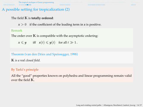
The field K is totally ordered:
x > 0 if the coefficient of the leading term in x is positive.
RemarkThe order over K is compatible with the asymptotic ordering:
x ⩽ y iff x(t) ⩽ y(t) for all t ≫ 1 .
Long and winding central paths | Allamigeon, Benchimol, Gaubert, Joswig | 13/37

Introduction The tropical analogue of linear programming Tropicalizing the central path Tropical lower bound on the complexity of IPMs Conclusion
A possible setting for tropicalizationThe entries of A, b and c are taken from a field K of “Puiseux series”.
DefinitionAn absolutely convergent generalized real Puiseux series is a series of the form:
x = c1tλ1 + c2tλ2 + . . . ,
where the ci are nonzero reals, and:• λ1 > λ2 > . . . is a strictly decreasing sequence of real numbers that is eitherfinite or unbounded;
• the series is absolutely convergent for t large enough.
The field K is totally ordered:
x > 0 if the coefficient of the leading term in x is positive.
RemarkThe order over K is compatible with the asymptotic ordering:
x ⩽ y iff x(t) ⩽ y(t) for all t ≫ 1 .
Long and winding central paths | Allamigeon, Benchimol, Gaubert, Joswig | 13/37

Introduction The tropical analogue of linear programming Tropicalizing the central path Tropical lower bound on the complexity of IPMs Conclusion
A possible setting for tropicalization (2)
The field K is totally ordered:x > 0 if the coefficient of the leading term in x is positive.
RemarkThe order over K is compatible with the asymptotic ordering:
x ⩽ y iff x(t) ⩽ y(t) for all t ≫ 1 .
Theorem (van den Dries and Speissegger, 1998)K is a real closed field.
By Tarki’s principleAll the “good” properties known on polyhedra and linear programming remain validover the field K.
=⇒ a LP over K encodes a parametric family of LPs over R:
minimize c⊤xsubject to Ax ⩽ b , x ∈ Kn
⩾0
minimize c(t)⊤xsubject to A(t)x ⩽ b(t) , x ∈ Rn
⩾0
Long and winding central paths | Allamigeon, Benchimol, Gaubert, Joswig | 14/37

Introduction The tropical analogue of linear programming Tropicalizing the central path Tropical lower bound on the complexity of IPMs Conclusion
A possible setting for tropicalization (2)
The field K is totally ordered:x > 0 if the coefficient of the leading term in x is positive.
RemarkThe order over K is compatible with the asymptotic ordering:
x ⩽ y iff x(t) ⩽ y(t) for all t ≫ 1 .
Theorem (van den Dries and Speissegger, 1998)K is a real closed field.
By Tarki’s principleAll the “good” properties known on polyhedra and linear programming remain validover the field K.
=⇒ a LP over K encodes a parametric family of LPs over R:
minimize c⊤xsubject to Ax ⩽ b , x ∈ Kn
⩾0
minimize c(t)⊤xsubject to A(t)x ⩽ b(t) , x ∈ Rn
⩾0Long and winding central paths | Allamigeon, Benchimol, Gaubert, Joswig | 14/37

Introduction The tropical analogue of linear programming Tropicalizing the central path Tropical lower bound on the complexity of IPMs Conclusion
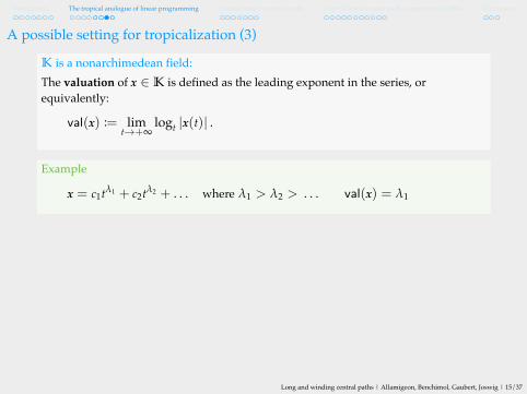
A possible setting for tropicalization (3)K is a nonarchimedean field:The valuation of x ∈ K is defined as the leading exponent in the series, orequivalently:
val(x) := limt→+∞
logt |x(t)| .
Example
x = c1tλ1 + c2tλ2 + . . . where λ1 > λ2 > . . . val(x) = λ1
The valuation maps the “classical” laws to the tropical ones:
∀x, y ∈ K⩾0,
val(x+ y) = max(val(x), val(y))val(x · y) = val(x) + val(y)
max(logt x(t), logt y(t)) ⩽ logt(x(t) + y(t)) ⩽ max(logt x(t), logt y(t)) + logt 2
logt(x(t) · y(t)) = logt x(t) + logt y(t)
Long and winding central paths | Allamigeon, Benchimol, Gaubert, Joswig | 15/37
Introduction The tropical analogue of linear programming Tropicalizing the central path Tropical lower bound on the complexity of IPMs Conclusion
A possible setting for tropicalization (3)K is a nonarchimedean field:The valuation of x ∈ K is defined as the leading exponent in the series, orequivalently:
val(x) := limt→+∞
logt |x(t)| .
Example
x = c1tλ1 + c2tλ2 + . . . where λ1 > λ2 > . . . val(x) = λ1
The valuation maps the “classical” laws to the tropical ones:
∀x, y ∈ K⩾0,
val(x+ y) = max(val(x), val(y))val(x · y) = val(x) + val(y)
max(logt x(t), logt y(t)) ⩽ logt(x(t) + y(t)) ⩽ max(logt x(t), logt y(t)) + logt 2
logt(x(t) · y(t)) = logt x(t) + logt y(t)
Long and winding central paths | Allamigeon, Benchimol, Gaubert, Joswig | 15/37

Introduction The tropical analogue of linear programming Tropicalizing the central path Tropical lower bound on the complexity of IPMs Conclusion
A possible setting for tropicalization (3)K is a nonarchimedean field:The valuation of x ∈ K is defined as the leading exponent in the series, orequivalently:
val(x) := limt→+∞
logt |x(t)| .
Example
x = c1tλ1 + c2tλ2 + . . . where λ1 > λ2 > . . . val(x) = λ1
The valuation maps the “classical” laws to the tropical ones:
∀x, y ∈ K⩾0,
val(x+ y) = max(val(x), val(y))val(x · y) = val(x) + val(y)
max(logt x(t), logt y(t)) ⩽ logt(x(t) + y(t)) ⩽ max(logt x(t), logt y(t)) + logt 2
logt(x(t) · y(t)) = logt x(t) + logt y(t)Long and winding central paths | Allamigeon, Benchimol, Gaubert, Joswig | 15/37

Introduction The tropical analogue of linear programming Tropicalizing the central path Tropical lower bound on the complexity of IPMs Conclusion
A possible setting for tropicalization (4)
Proposition (Develin and Yu, 2007)LetP ⊂ Kn
⩾0 be a convex polyhedron. Then val(P) is a tropical polyhedron.
Every polyhedronP := x ∈ Kn⩾0 : Ax ⩽ b gives rise to a parametric family of real
convex polyhedra:
P(t) :=x ∈ Rn
⩾0 : A(t)x ⩽ b(t)
.
Theorem
val(P) = limt→+∞
logt(P(t)) .
Moreover, when the entries of A and b are monomials, we have
d(logt P(t), val(P)) ⩽ logt((n+ 1)2(n!)4
)provided that t is large enough.
Long and winding central paths | Allamigeon, Benchimol, Gaubert, Joswig | 16/37

Introduction The tropical analogue of linear programming Tropicalizing the central path Tropical lower bound on the complexity of IPMs Conclusion
Outline of the talk
1 The tropical analogue of linear programming
2 Tropicalizing the central path
3 Tropical lower bound on the complexity of IPMs
4 Conclusion
Long and winding central paths | Allamigeon, Benchimol, Gaubert, Joswig | 17/37

Introduction The tropical analogue of linear programming Tropicalizing the central path Tropical lower bound on the complexity of IPMs Conclusion
The central path over Puiseux series
Given A ∈ Km×n, b ∈ Km and c ∈ Kn, consider the following LP:minimize c⊤xsubject to Ax ⩽ b , x ⩾ 0
, w ⩾ 0
LP(A, b, c)
and its dual:maximize −b⊤ysubject to −A⊤y+ s = c , s ⩾ 0 , y ⩾ 0
DualLP(A, b, c)
Proposition-DefinitionUnder mild conditions, for all µ ∈ K>0, the system
Ax+w = b−A⊤y+ s = c
∀j, xjsj = µ
∀i, wiyi = µ
has a unique solution C(µ) = (xµ,wµ, sµ, yµ)
which is called the primal-dual centralpath at µ.
“µ-perturbed” optimality conditions
Long and winding central paths | Allamigeon, Benchimol, Gaubert, Joswig | 18/37

Introduction The tropical analogue of linear programming Tropicalizing the central path Tropical lower bound on the complexity of IPMs Conclusion
The central path over Puiseux series
Given A ∈ Km×n, b ∈ Km and c ∈ Kn, consider the following LP:minimize c⊤xsubject to Ax+w = b , x ⩾ 0 , w ⩾ 0
LP(A, b, c)
and its dual:maximize −b⊤ysubject to −A⊤y+ s = c , s ⩾ 0 , y ⩾ 0
DualLP(A, b, c)
Proposition-DefinitionUnder mild conditions, for all µ ∈ K>0, the system
Ax+w = b−A⊤y+ s = c
∀j, xjsj = µ
∀i, wiyi = µ
has a unique solution C(µ) = (xµ,wµ, sµ, yµ)
which is called the primal-dual centralpath at µ.
“µ-perturbed” optimality conditions
Long and winding central paths | Allamigeon, Benchimol, Gaubert, Joswig | 18/37

Introduction The tropical analogue of linear programming Tropicalizing the central path Tropical lower bound on the complexity of IPMs Conclusion
The central path over Puiseux series
Given A ∈ Rm×n, b ∈ Rm and c ∈ Rn, consider the following LP:minimize c⊤xsubject to Ax+w = b , x ⩾ 0 , w ⩾ 0
LP(A, b, c)
and its dual:maximize −b⊤ysubject to −A⊤y+ s = c , s ⩾ 0 , y ⩾ 0
DualLP(A, b, c)
Proposition-DefinitionUnder mild conditions, for all µ ∈ R>0, the system
Ax+w = b−A⊤y+ s = c
∀j, xjsj = µ
∀i, wiyi = µ
has a unique solution C(µ) = (xµ,wµ, sµ, yµ) which is called the primal-dual centralpath at µ.
“µ-perturbed” optimality conditions
Long and winding central paths | Allamigeon, Benchimol, Gaubert, Joswig | 18/37

Introduction The tropical analogue of linear programming Tropicalizing the central path Tropical lower bound on the complexity of IPMs Conclusion
The central path over Puiseux series
Given A ∈ Km×n, b ∈ Km and c ∈ Kn, consider the following LP:minimize c⊤xsubject to Ax+w = b , x ⩾ 0 , w ⩾ 0
LP(A, b, c)
and its dual:maximize −b⊤ysubject to −A⊤y+ s = c , s ⩾ 0 , y ⩾ 0
DualLP(A, b, c)
Proposition-DefinitionUnder mild conditions, for all µ ∈ K>0, the system
Ax+w = b−A⊤y+ s = c
∀j, xjsj = µ
∀i, wiyi = µ
has a unique solution C(µ) = (xµ,wµ, sµ, yµ) which is called the primal-dual centralpath at µ.
“µ-perturbed” optimality conditions
Long and winding central paths | Allamigeon, Benchimol, Gaubert, Joswig | 18/37
Introduction The tropical analogue of linear programming Tropicalizing the central path Tropical lower bound on the complexity of IPMs Conclusion
The tropical central path
Natural question: what is the image under the valuation of the central path?
Relies on the notion of barycenter of a (compact)tropical polyhedron P= greatest point of the set P w.r.t. thecoordinate-wise order⩽
LetP be the feasible set of LP(A, b, c):
P := (x,w) ∈ Kn+m⩾0 : Ax+w = b .
Assume, for simplicity, b, c ⩾ 0.
TheoremThe image under val of the point (xµ,wµ) of the primal central path is given by thebarycenter of the tropical polyhedron:
val(P) ∩ (x,w) ∈ Tn+m : val(c)⊤ ⊙ x ⩽ val(µ) .
Long and winding central paths | Allamigeon, Benchimol, Gaubert, Joswig | 19/37

Introduction The tropical analogue of linear programming Tropicalizing the central path Tropical lower bound on the complexity of IPMs Conclusion
The tropical central path (2)
LetP be the feasible set of LP(A, b, c).Assume, for simplicity, b, c ⩾ 0.
TheoremThe image under val of the point (xµ,wµ) of the primal central path is given by thebarycenter of the tropical polyhedron:
val(P) ∩ (x,w) ∈ Tn+m : val(c)⊤ ⊙ x ⩽ val(µ) .
The image under val of the point (sµ, yµ) of the dual central path is given by the barycenter ofthe tropical polyhedron:
val(Q) ∩ (s, y) ∈ Tn+m : val(b)⊤ ⊙ y ⩽ val(µ) .
=⇒ yields a tropical central path λ 7→ C trop(λ):C trop(λ) := val(C(µ)) for any µ such that val(µ) = λ .
RemarkThe tropical central path does not depend on the representation ofP andQ.
Long and winding central paths | Allamigeon, Benchimol, Gaubert, Joswig | 20/37

Introduction The tropical analogue of linear programming Tropicalizing the central path Tropical lower bound on the complexity of IPMs Conclusion
The tropical central path (2)
LetP be the feasible set of LP(A, b, c) andQ be the feasible set of DualLP(A, b, c).Assume, for simplicity, b, c ⩾ 0.
TheoremThe image under val of the point (xµ,wµ) of the primal central path is given by thebarycenter of the tropical polyhedron:
val(P) ∩ (x,w) ∈ Tn+m : val(c)⊤ ⊙ x ⩽ val(µ) .
The image under val of the point (sµ, yµ) of the dual central path is given by the barycenter ofthe tropical polyhedron:
val(Q) ∩ (s, y) ∈ Tn+m : val(b)⊤ ⊙ y ⩽ val(µ) .
=⇒ yields a tropical central path λ 7→ C trop(λ):C trop(λ) := val(C(µ)) for any µ such that val(µ) = λ .
RemarkThe tropical central path does not depend on the representation ofP andQ.
Long and winding central paths | Allamigeon, Benchimol, Gaubert, Joswig | 20/37

Introduction The tropical analogue of linear programming Tropicalizing the central path Tropical lower bound on the complexity of IPMs Conclusion
Example
minimize x1 + t3x2
P :
x1 + x2 ⩽ 2tx1 ⩽ 1+ t2x2tx2 ⩽ 1+ t3x1x1 ⩽ t2x2
x1, x2 ⩾ 0
max(x1, 3+ x2) ⩽ λ
val(P) :
max(x1, x2) ⩽ 01+ x1 ⩽ max(0, 2+ x2)1+ x2 ⩽ max(0, 3+ x1)
x1 ⩽ 2+ x2
λ = 4λ = 3λ = 2λ = 1λ = 0λ = −1
Long and winding central paths | Allamigeon, Benchimol, Gaubert, Joswig | 21/37

Introduction The tropical analogue of linear programming Tropicalizing the central path Tropical lower bound on the complexity of IPMs Conclusion
Exampleminimize x1 + t3x2
P :
x1 + x2 ⩽ 2tx1 ⩽ 1+ t2x2tx2 ⩽ 1+ t3x1x1 ⩽ t2x2
x1, x2 ⩾ 0
max(x1, 3+ x2)
⩽ λ
val(P) :
max(x1, x2) ⩽ 01+ x1 ⩽ max(0, 2+ x2)1+ x2 ⩽ max(0, 3+ x1)
x1 ⩽ 2+ x2
λ = 4λ = 3λ = 2λ = 1λ = 0λ = −1
Long and winding central paths | Allamigeon, Benchimol, Gaubert, Joswig | 21/37

Introduction The tropical analogue of linear programming Tropicalizing the central path Tropical lower bound on the complexity of IPMs Conclusion
Exampleminimize x1 + t3x2
P :
x1 + x2 ⩽ 2tx1 ⩽ 1+ t2x2tx2 ⩽ 1+ t3x1x1 ⩽ t2x2
x1, x2 ⩾ 0
max(x1, 3+ x2) ⩽ λ
val(P) :
max(x1, x2) ⩽ 01+ x1 ⩽ max(0, 2+ x2)1+ x2 ⩽ max(0, 3+ x1)
x1 ⩽ 2+ x2
λ = 4λ = 3λ = 2λ = 1λ = 0λ = −1
Long and winding central paths | Allamigeon, Benchimol, Gaubert, Joswig | 21/37

Introduction The tropical analogue of linear programming Tropicalizing the central path Tropical lower bound on the complexity of IPMs Conclusion
Exampleminimize x1 + t3x2
P :
x1 + x2 ⩽ 2tx1 ⩽ 1+ t2x2tx2 ⩽ 1+ t3x1x1 ⩽ t2x2
x1, x2 ⩾ 0
max(x1, 3+ x2) ⩽ λ
val(P) :
max(x1, x2) ⩽ 01+ x1 ⩽ max(0, 2+ x2)1+ x2 ⩽ max(0, 3+ x1)
x1 ⩽ 2+ x2
λ = 4
λ = 3λ = 2λ = 1λ = 0λ = −1
Long and winding central paths | Allamigeon, Benchimol, Gaubert, Joswig | 21/37

Introduction The tropical analogue of linear programming Tropicalizing the central path Tropical lower bound on the complexity of IPMs Conclusion
Exampleminimize x1 + t3x2
P :
x1 + x2 ⩽ 2tx1 ⩽ 1+ t2x2tx2 ⩽ 1+ t3x1x1 ⩽ t2x2
x1, x2 ⩾ 0
max(x1, 3+ x2) ⩽ λ
val(P) :
max(x1, x2) ⩽ 01+ x1 ⩽ max(0, 2+ x2)1+ x2 ⩽ max(0, 3+ x1)
x1 ⩽ 2+ x2
λ = 4
λ = 3
λ = 2λ = 1λ = 0λ = −1
Long and winding central paths | Allamigeon, Benchimol, Gaubert, Joswig | 21/37

Introduction The tropical analogue of linear programming Tropicalizing the central path Tropical lower bound on the complexity of IPMs Conclusion
Exampleminimize x1 + t3x2
P :
x1 + x2 ⩽ 2tx1 ⩽ 1+ t2x2tx2 ⩽ 1+ t3x1x1 ⩽ t2x2
x1, x2 ⩾ 0
max(x1, 3+ x2) ⩽ λ
val(P) :
max(x1, x2) ⩽ 01+ x1 ⩽ max(0, 2+ x2)1+ x2 ⩽ max(0, 3+ x1)
x1 ⩽ 2+ x2
λ = 4λ = 3
λ = 2
λ = 1λ = 0λ = −1
Long and winding central paths | Allamigeon, Benchimol, Gaubert, Joswig | 21/37

Introduction The tropical analogue of linear programming Tropicalizing the central path Tropical lower bound on the complexity of IPMs Conclusion
Exampleminimize x1 + t3x2
P :
x1 + x2 ⩽ 2tx1 ⩽ 1+ t2x2tx2 ⩽ 1+ t3x1x1 ⩽ t2x2
x1, x2 ⩾ 0
max(x1, 3+ x2) ⩽ λ
val(P) :
max(x1, x2) ⩽ 01+ x1 ⩽ max(0, 2+ x2)1+ x2 ⩽ max(0, 3+ x1)
x1 ⩽ 2+ x2
λ = 4λ = 3λ = 2
λ = 1
λ = 0λ = −1
Long and winding central paths | Allamigeon, Benchimol, Gaubert, Joswig | 21/37

Introduction The tropical analogue of linear programming Tropicalizing the central path Tropical lower bound on the complexity of IPMs Conclusion
Exampleminimize x1 + t3x2
P :
x1 + x2 ⩽ 2tx1 ⩽ 1+ t2x2tx2 ⩽ 1+ t3x1x1 ⩽ t2x2
x1, x2 ⩾ 0
max(x1, 3+ x2) ⩽ λ
val(P) :
max(x1, x2) ⩽ 01+ x1 ⩽ max(0, 2+ x2)1+ x2 ⩽ max(0, 3+ x1)
x1 ⩽ 2+ x2
λ = 4λ = 3λ = 2λ = 1
λ = 0
λ = −1
Long and winding central paths | Allamigeon, Benchimol, Gaubert, Joswig | 21/37

Introduction The tropical analogue of linear programming Tropicalizing the central path Tropical lower bound on the complexity of IPMs Conclusion
Exampleminimize x1 + t3x2
P :
x1 + x2 ⩽ 2tx1 ⩽ 1+ t2x2tx2 ⩽ 1+ t3x1x1 ⩽ t2x2
x1, x2 ⩾ 0
max(x1, 3+ x2) ⩽ λ
val(P) :
max(x1, x2) ⩽ 01+ x1 ⩽ max(0, 2+ x2)1+ x2 ⩽ max(0, 3+ x1)
x1 ⩽ 2+ x2
λ = 4λ = 3λ = 2λ = 1λ = 0
λ = −1Long and winding central paths | Allamigeon, Benchimol, Gaubert, Joswig | 21/37

Introduction The tropical analogue of linear programming Tropicalizing the central path Tropical lower bound on the complexity of IPMs Conclusion
Exampleminimize x1 + t3x2
P :
x1 + x2 ⩽ 2tx1 ⩽ 1+ t2x2tx2 ⩽ 1+ t3x1x1 ⩽ t2x2
x1, x2 ⩾ 0
max(x1, 3+ x2) ⩽ λ
val(P) :
max(x1, x2) ⩽ 01+ x1 ⩽ max(0, 2+ x2)1+ x2 ⩽ max(0, 3+ x1)
x1 ⩽ 2+ x2
λ = 4λ = 3λ = 2λ = 1λ = 0λ = −1
Long and winding central paths | Allamigeon, Benchimol, Gaubert, Joswig | 21/37

Introduction The tropical analogue of linear programming Tropicalizing the central path Tropical lower bound on the complexity of IPMs Conclusion
Pathological example of tropical central path
minimize x1subject to x1 ⩽ t2
x2 ⩽ tx2j+1 ⩽ t x2j−1 , x2j+1 ⩽ t x2jx2j+2 ⩽ t1−1/2j (x2j−1 + x2j)x2r−1 ⩾ 0 , x2r ⩾ 0
1 ⩽ j < r
Tropical central pathThe x-component of C trop(λ) is given by
xλ1 = min(λ, 2)
xλ2 = 1
xλ2j+1 = 1+ min(xλ
2j−1, xλ2j)
xλ2j+2 = (1− 1/2j) + max(xλ
2j−1, xλ2j)
1 ⩽ j < r
0 1 20
1
2
3
4
5
λ
xλ1
xλ2
xλ3
xλ4
xλ5
xλ6
xλ7
xλ8
xλ9
xλ10
Long and winding central paths | Allamigeon, Benchimol, Gaubert, Joswig | 22/37

Introduction The tropical analogue of linear programming Tropicalizing the central path Tropical lower bound on the complexity of IPMs Conclusion
Pathological example of tropical central path
minimize x1subject to x1 ⩽ t2
x2 ⩽ tx2j+1 ⩽ t x2j−1 , x2j+1 ⩽ t x2jx2j+2 ⩽ t1−1/2j (x2j−1 + x2j)x2r−1 ⩾ 0 , x2r ⩾ 0
1 ⩽ j < r
Tropical central pathThe x-component of C trop(λ) is the greatest point of
x1 ⩽ λ
x1 ⩽ 2 , x2 ⩽ 1x2j+1 ⩽ 1+ x2j−1 , x2j+1 ⩽ 1+ x2jx2j+2 ⩽ (1− 1/2j) + max(x2j−1, x2j)
1 ⩽ j < r ,
0 1 20
1
2
3
4
5
λ
xλ1
xλ2
xλ3
xλ4
xλ5
xλ6
xλ7
xλ8
xλ9
xλ10
Long and winding central paths | Allamigeon, Benchimol, Gaubert, Joswig | 22/37

Introduction The tropical analogue of linear programming Tropicalizing the central path Tropical lower bound on the complexity of IPMs Conclusion
Pathological example of tropical central path
minimize x1subject to x1 ⩽ t2
x2 ⩽ tx2j+1 ⩽ t x2j−1 , x2j+1 ⩽ t x2jx2j+2 ⩽ t1−1/2j (x2j−1 + x2j)x2r−1 ⩾ 0 , x2r ⩾ 0
1 ⩽ j < r
Tropical central pathThe x-component of C trop(λ) is given by
xλ1 = min(λ, 2)
xλ2 = 1
xλ2j+1 = 1+ min(xλ
2j−1, xλ2j)
xλ2j+2 = (1− 1/2j) + max(xλ
2j−1, xλ2j)
1 ⩽ j < r
0 1 20
1
2
3
4
5
λ
xλ1
xλ2
xλ3
xλ4
xλ5
xλ6
xλ7
xλ8
xλ9
xλ10
Long and winding central paths | Allamigeon, Benchimol, Gaubert, Joswig | 22/37

Introduction The tropical analogue of linear programming Tropicalizing the central path Tropical lower bound on the complexity of IPMs Conclusion
Pathological example of tropical central path
minimize x1subject to x1 ⩽ t2
x2 ⩽ tx2j+1 ⩽ t x2j−1 , x2j+1 ⩽ t x2jx2j+2 ⩽ t1−1/2j (x2j−1 + x2j)x2r−1 ⩾ 0 , x2r ⩾ 0
1 ⩽ j < r
Tropical central pathThe x-component of C trop(λ) is given by
xλ1 = min(λ, 2)
xλ2 = 1
xλ2j+1 = 1+ min(xλ
2j−1, xλ2j)
xλ2j+2 = (1− 1/2j) + max(xλ
2j−1, xλ2j)
1 ⩽ j < r
0 1 20
1
2
3
4
5
λ
xλ1
xλ2
xλ3
xλ4
xλ5
xλ6
xλ7
xλ8
xλ9
xλ10
Long and winding central paths | Allamigeon, Benchimol, Gaubert, Joswig | 22/37
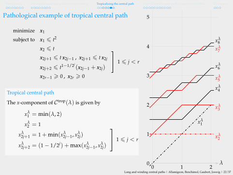
Introduction The tropical analogue of linear programming Tropicalizing the central path Tropical lower bound on the complexity of IPMs Conclusion
Pathological example of tropical central path
minimize x1subject to x1 ⩽ t2
x2 ⩽ tx2j+1 ⩽ t x2j−1 , x2j+1 ⩽ t x2jx2j+2 ⩽ t1−1/2j (x2j−1 + x2j)x2r−1 ⩾ 0 , x2r ⩾ 0
1 ⩽ j < r
Tropical central pathThe x-component of C trop(λ) is given by
xλ1 = min(λ, 2)
xλ2 = 1
xλ2j+1 = 1+ min(xλ
2j−1, xλ2j)
xλ2j+2 = (1− 1/2j) + max(xλ
2j−1, xλ2j)
1 ⩽ j < r
0 1 20
1
2
3
4
5
λ
xλ1
xλ2
xλ3
xλ4
xλ5
xλ6
xλ7
xλ8
xλ9
xλ10
Long and winding central paths | Allamigeon, Benchimol, Gaubert, Joswig | 22/37

Introduction The tropical analogue of linear programming Tropicalizing the central path Tropical lower bound on the complexity of IPMs Conclusion
Pathological example of tropical central pathProjection onto the (x2r−1, x2r)-plane: staircase with 2r−1 steps
x2r−1
x2r
r− 1r− 1(r− 1)
+ 22r−1
(r− 1)+ 4
2r−1
(r− 1)+ 6
2r−1
(r− 1)+ 1
2r−1
(r− 1)+ 3
2r−1
(r− 1)+ 5
2r−1
(r− 1)+ 7
2r−1
λ = 0λ = 1
2r−2
λ = 22r−2
λ = 32r−2
λ = 42r−2
λ = 52r−2
λ = 62r−2
Long and winding central paths | Allamigeon, Benchimol, Gaubert, Joswig | 23/37

Introduction The tropical analogue of linear programming Tropicalizing the central path Tropical lower bound on the complexity of IPMs Conclusion
Outline of the talk
1 The tropical analogue of linear programming
2 Tropicalizing the central path
3 Tropical lower bound on the complexity of IPMs
4 Conclusion
Long and winding central paths | Allamigeon, Benchimol, Gaubert, Joswig | 24/37

Introduction The tropical analogue of linear programming Tropicalizing the central path Tropical lower bound on the complexity of IPMs Conclusion
Classical central path vs tropical central
So far, we looked at the central path of the linear program LP(A, b, c) over Puiseuxseries:
µ ∈ K>0 7→ C(µ)
Associated family of (real) central pathsCentral path of
LP(A(t), b(t), c(t)) ≡ minc(t)⊤x : A(t)x+ w = b(t) , x,w ⩾ 0
denoted by
µ ∈ R>0 7→ Ct(µ)
QuestionConvergence of the image under logt of:• the family of central paths Ct
• the neighborhood of these central paths
to the tropical central path?
Long and winding central paths | Allamigeon, Benchimol, Gaubert, Joswig | 25/37

Introduction The tropical analogue of linear programming Tropicalizing the central path Tropical lower bound on the complexity of IPMs Conclusion
Classical central path vs tropical central
So far, we looked at the central path of the linear program LP(A, b, c) over Puiseuxseries:
µ ∈ K>0 7→ C(µ)
Associated family of (real) central pathsCentral path of
LP(A(t), b(t), c(t)) ≡ minc(t)⊤x : A(t)x+ w = b(t) , x,w ⩾ 0
denoted by
µ ∈ R>0 7→ Ct(µ)
QuestionConvergence of the image under logt of:• the family of central paths Ct
• the neighborhood of these central paths
to the tropical central path?Long and winding central paths | Allamigeon, Benchimol, Gaubert, Joswig | 25/37

Introduction The tropical analogue of linear programming Tropicalizing the central path Tropical lower bound on the complexity of IPMs Conclusion
Classical central path vs tropical central
So far, we looked at the central path of the linear program LP(A, b, c) over Puiseuxseries:
µ ∈ K>0 7→ C(µ)
Associated family of (real) central pathsCentral path of
LP(A(t), b(t), c(t)) ≡ minc(t)⊤x : A(t)x+ w = b(t) , x,w ⩾ 0
denoted by
µ ∈ R>0 7→ Ct(µ)
QuestionConvergence of the image under logt of:• the family of central paths Ct• the neighborhood of these central paths
to the tropical central path?Long and winding central paths | Allamigeon, Benchimol, Gaubert, Joswig | 25/37

Introduction The tropical analogue of linear programming Tropicalizing the central path Tropical lower bound on the complexity of IPMs Conclusion
Neighborhoods of the classical central
Several kinds of neighborhoods used by interior point methods, which result indifferent complexity bounds.
We consider the widest kind of neighborhoods studied in the literature:
N−∞t (µ) :=
(x,w, s, y) ∈ P(t)×Q(t) : µ(x,w, s, y) = µ
and ( xswy ) ⩾ (1− θ)µe
where θ ∈ ]0, 1[ parametrizes the size of the neighborhood, and:
• µ(x,w, s, y) := 1m+n
(x⊤s+ w⊤y
)• e is the all-1 vector.
To summarizeN−∞
t (µ) is a neighborhood of the point Ct(µ) of the central path of
LP(A(t), b(t), c(t)) ≡ minc(t)⊤x | A(t)x+ w = b(t) , x,w ⩾ 0 .
and θ is a fixed parameter in ]0, 1[ related to the size of the neighborhood.
Long and winding central paths | Allamigeon, Benchimol, Gaubert, Joswig | 26/37

Introduction The tropical analogue of linear programming Tropicalizing the central path Tropical lower bound on the complexity of IPMs Conclusion
Neighborhoods of the classical central
Several kinds of neighborhoods used by interior point methods, which result indifferent complexity bounds.
We consider the widest kind of neighborhoods studied in the literature:
N−∞t (µ) :=
(x,w, s, y) ∈ P(t)×Q(t) : µ(x,w, s, y) = µ
and ( xswy ) ⩾ (1− θ)µe
where θ ∈ ]0, 1[ parametrizes the size of the neighborhood, and:• µ(x,w, s, y) := 1
m+n(x⊤s+ w⊤y
)• e is the all-1 vector.
To summarizeN−∞
t (µ) is a neighborhood of the point Ct(µ) of the central path of
LP(A(t), b(t), c(t)) ≡ minc(t)⊤x | A(t)x+ w = b(t) , x,w ⩾ 0 .
and θ is a fixed parameter in ]0, 1[ related to the size of the neighborhood.
Long and winding central paths | Allamigeon, Benchimol, Gaubert, Joswig | 26/37

Introduction The tropical analogue of linear programming Tropicalizing the central path Tropical lower bound on the complexity of IPMs Conclusion
Uniform convergence to the tropical central
TheoremThe image under logt of the neighborhoods of the central paths
(Ct(·)
)t≫1 uniformly
converges to the tropical central path:
∀µ ∈ R>0 , d∞(logt N−∞t (µ) , C trop(logt µ)) ⩽ logt
(m+ n1− θ
)+ δ(t) .
RemarkThe quantity δ(t) is built from the Hausdorff distance between the sets logt P(t) andvalP and their dual counterparts.
Long and winding central paths | Allamigeon, Benchimol, Gaubert, Joswig | 27/37

Introduction The tropical analogue of linear programming Tropicalizing the central path Tropical lower bound on the complexity of IPMs Conclusion
Uniform convergence to the tropical central (2)
ε
For all radius ε > 0, if t is sufficiently large, we have
logt( )
⊂
Long and winding central paths | Allamigeon, Benchimol, Gaubert, Joswig | 28/37

Introduction The tropical analogue of linear programming Tropicalizing the central path Tropical lower bound on the complexity of IPMs Conclusion
Pathological tropical central pathIn the (x2r−1, x2r)-plane,
x2r−1
x2r
For t sufficiently large:• the image under logt of the pointsarising in the iterations of the IPM
• as well as the image under logt of thesegments between successive points
• as well as the sequence of tropicalsegments between successive points
are contained in the neighborhood of thetropical central path.
Long and winding central paths | Allamigeon, Benchimol, Gaubert, Joswig | 29/37
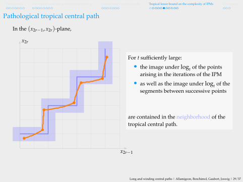

Introduction The tropical analogue of linear programming Tropicalizing the central path Tropical lower bound on the complexity of IPMs Conclusion
Classical and tropical segmentsDefinitionGiven x, y ∈ Tn, the tropical segment between x and y is defined as:
tsegm(x, y) :=(
λ ⊙ x)⊕(µ ⊙ y
)| λ ⊕ µ = 0
.
PropositionGiven x, y ∈ Kn
⩾0,
d∞
(logt
[x(t), y(t)
], tsegm
((logt x(t), logt y(t)
))= O
( 1log t
).
Long and winding central paths | Allamigeon, Benchimol, Gaubert, Joswig | 30/37

Introduction The tropical analogue of linear programming Tropicalizing the central path Tropical lower bound on the complexity of IPMs Conclusion
Pathological tropical central path (2)In the (x2r−1, x2r)-plane,
x2r−1
x2r
For t sufficiently large:• the image under logt of the pointsarising in the iterations of the IPM
• as well as the image under logt of thesegments between successive points
• as well as the sequence of tropicalsegments between successive points
are contained in the neighborhood of thetropical central path.
Long and winding central paths | Allamigeon, Benchimol, Gaubert, Joswig | 31/37

Introduction The tropical analogue of linear programming Tropicalizing the central path Tropical lower bound on the complexity of IPMs Conclusion
Pathological tropical central path (3)
Let us set the radius of the neighborhood to ε < 12r+1 .
x2r−1
x2r
There is no tropical segment contained inthe neighborhood between any two pointsin distinct red parts.
There is no tropical segment contained inthe neighborhood between any two pointsin distinct green parts.
=⇒ in the best case, points have to al-ternate between successive red andgreen parts.
Long and winding central paths | Allamigeon, Benchimol, Gaubert, Joswig | 32/37
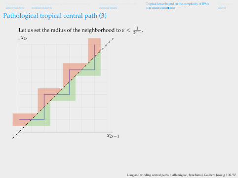
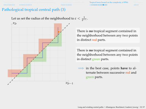
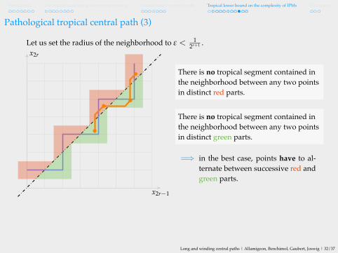
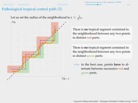

Introduction The tropical analogue of linear programming Tropicalizing the central path Tropical lower bound on the complexity of IPMs Conclusion
Tropical lower bound on the number of iterations (2)
LemmaThe tropical central path is a union of tropical segments.
γ([λ, λ]) := smallest number of tropical segments needed to describe C trop([λ, λ]).
PropositionLet tsegm(z0, z1) ∪ · · · ∪ tsegm(zp−1, zp) be asequence of tropical segments contained in theneighborhood∪
λ⩽λ⩽λ
B∞(C trop(λ); ϵ)
of C trop([λ, λ]), and such that
z0 ∈ B∞(C trop(λ)) , zp ∈ B∞(C trop(λ)) .
If ϵ ≪ 1, we have p ⩾ γ([λ, λ]).
z6
z5z4
z3
z2
z1
z0
C trop(λ)
C trop(λ)
Long and winding central paths | Allamigeon, Benchimol, Gaubert, Joswig | 33/37

Introduction The tropical analogue of linear programming Tropicalizing the central path Tropical lower bound on the complexity of IPMs Conclusion
Application to the pathological tropical central path
minimize x1subject to x1 ⩽ t2
x2 ⩽ tx2j+1 ⩽ t x2j−1 , x2j+1 ⩽ t x2jx2j+2 ⩽ t1−1/2j (x2j−1 + x2j)x2r−1 ⩾ 0 , x2r ⩾ 0
1 ⩽ j < r
LWr(t) x2r−1
x2r
CorollaryLet 0 < θ < 1, and suppose that
t >((
(10r− 1)!)8
1− θ
)2r+2
.
Then, any log-barrier interior point method which describes a trajectory contained in theneighborhoodN−∞
θ,t of the primal-dual central path of LWr(t), needs to perform at least 2r−1
iterations to reduce the duality measure from t2 to 1.
Long and winding central paths | Allamigeon, Benchimol, Gaubert, Joswig | 34/37

Introduction The tropical analogue of linear programming Tropicalizing the central path Tropical lower bound on the complexity of IPMs Conclusion
Application to the pathological tropical central path
minimize x1subject to x1 ⩽ t2
x2 ⩽ tx2j+1 ⩽ t x2j−1 , x2j+1 ⩽ t x2jx2j+2 ⩽ t1−1/2j (x2j−1 + x2j)x2r−1 ⩾ 0 , x2r ⩾ 0
1 ⩽ j < r
LWr(t) x2r−1
x2r
TheoremLet 0 < θ < 1, and suppose that
t >((
(10r− 1)!)8
1− θ
)2r+2
.
Then, every polygonal curve [z0, z1] ∪ [z1, z2] ∪ · · · ∪ [zp−1, zp] contained in theneighborhoodN−∞
θ,t of the primal-dual central path of LWr(t), with µ(z0) ⩽ 1 andµ(zp) ⩾ t2, contains at least 2r−1 segments.
CorollaryLet 0 < θ < 1, and suppose that
t >((
(10r− 1)!)8
1− θ
)2r+2
.
Then, any log-barrier interior point method which describes a trajectory contained in theneighborhoodN−∞
θ,t of the primal-dual central path of LWr(t), needs to perform at least 2r−1
iterations to reduce the duality measure from t2 to 1.
Long and winding central paths | Allamigeon, Benchimol, Gaubert, Joswig | 34/37

Introduction The tropical analogue of linear programming Tropicalizing the central path Tropical lower bound on the complexity of IPMs Conclusion
Application to the pathological tropical central path
minimize x1subject to x1 ⩽ t2
x2 ⩽ tx2j+1 ⩽ t x2j−1 , x2j+1 ⩽ t x2jx2j+2 ⩽ t1−1/2j (x2j−1 + x2j)x2r−1 ⩾ 0 , x2r ⩾ 0
1 ⩽ j < r
LWr(t) x2r−1
x2r
CorollaryLet 0 < θ < 1, and suppose that
t >((
(10r− 1)!)8
1− θ
)2r+2
.
Then, any log-barrier interior point method which describes a trajectory contained in theneighborhoodN−∞
θ,t of the primal-dual central path of LWr(t), needs to perform at least 2r−1
iterations to reduce the duality measure from t2 to 1.Long and winding central paths | Allamigeon, Benchimol, Gaubert, Joswig | 34/37

Introduction The tropical analogue of linear programming Tropicalizing the central path Tropical lower bound on the complexity of IPMs Conclusion
Outline of the talk
1 The tropical analogue of linear programming
2 Tropicalizing the central path
3 Tropical lower bound on the complexity of IPMs
4 Conclusion
Long and winding central paths | Allamigeon, Benchimol, Gaubert, Joswig | 35/37
Introduction The tropical analogue of linear programming Tropicalizing the central path Tropical lower bound on the complexity of IPMs Conclusion
Conclusion
Contribution
• we have used tropical geometry to analyze the complexity of log-barrier interiorpoints
• evaluate the complexity of algorithms over numerical instances with differentorders of magnitude
PerspectivesCan we generalize this approach?• other barrier functions• other optimization problems
Can we fix interior point methods?
Long and winding central paths | Allamigeon, Benchimol, Gaubert, Joswig | 36/37

Thank you!
Log-barrier interior point methods are not strongly polynomial, arXiv:1708.01544

Introduction The tropical analogue of linear programming Tropicalizing the central path Tropical lower bound on the complexity of IPMs Conclusion
D. A. Bayer and J. C. Lagarias. The nonlinear geometry of linear programming. I.Affine and projective scaling trajectories. Trans. Amer. Math. Soc., 314(2):499–526,1989. ISSN 0002-9947. doi: 10.2307/2001396. URLhttp://dx.doi.org/10.2307/2001396.
J.A. De Loera, B. Sturmfels, and C. Vinzant. The central curve in linear programming.Foundations of Computational Mathematics, 12(4):509–540, 2012.
J.-P. Dedieu and M. Shub. Newton flow and interior point methods in linearprogramming. International Journal of Bifurcation and Chaos, 15(03):827–839,2005.
J.-P. Dedieu, G. Malajovich, and M. Shub. On the curvature of the central path oflinear programming theory. Foundations of Computational Mathematics, 5(2):145–171, 2005.
M. Develin and J. Yu. Tropical polytopes and cellular resolutions. Experiment. Math.,16(3):277–291, 2007. ISSN 1058-6458.
A. Deza, T. Terlaky, and Y. Zinchenko. Central path curvature anditeration-complexity for redundant Klee-Minty cubes. In Advances in appliedmathematics and global optimization, volume 17 of Adv. Mech. Math., pages223–256. Springer, New York, 2009. doi: 10.1007/978-0-387-75714-8_7. URLhttp://dx.doi.org/10.1007/978-0-387-75714-8_7.
N. Karmarkar. A new polynomial-time algorithm for linear programming.Combinatorica, 4(4):373–395, December 1984. ISSN 0209-9683. doi:10.1007/BF02579150. URL http://dx.doi.org/10.1007/BF02579150.
Long and winding central paths | Allamigeon, Benchimol, Gaubert, Joswig | 37/37

Introduction The tropical analogue of linear programming Tropicalizing the central path Tropical lower bound on the complexity of IPMs Conclusion
L.G. Khachiyan. Polynomial algorithms in linear programming. USSRComputational Mathematics and Mathematical Physics, 20(1):53–72, 1980. ISSN0041-5553. doi: http://dx.doi.org/10.1016/0041-5553(80)90061-0.
L. van den Dries and P. Speissegger. The real field with convergent generalized powerseries. Trans. Amer. Math. Soc., 350(11):4377–4421, 1998. ISSN 0002-9947. doi:10.1090/S0002-9947-98-02105-9. URLhttp://dx.doi.org/10.1090/S0002-9947-98-02105-9.
Long and winding central paths | Allamigeon, Benchimol, Gaubert, Joswig | 37/37