Forschungsinstitut zur Zukunft der ArbeitInstitute for the Study of Labor

DI

SC

US

SI

ON

P

AP

ER

S

ER

IE

S

Long-Lasting Effects of Socialist Education

IZA DP No. 9678

January 2016

Nicola Fuchs-SchündelnPaolo Masella

Long-Lasting Effects of

Socialist Education

Nicola Fuchs-Schündeln Goethe University Frankfurt,

CEPR and IZA

Paolo Masella University of Sussex

and IZA

Discussion Paper No. 9678 January 2016

IZA

P.O. Box 7240 53072 Bonn

Germany

Phone: +49-228-3894-0 Fax: +49-228-3894-180

E-mail: iza@iza.org

Any opinions expressed here are those of the author(s) and not those of IZA. Research published in this series may include views on policy, but the institute itself takes no institutional policy positions. The IZA research network is committed to the IZA Guiding Principles of Research Integrity. The Institute for the Study of Labor (IZA) in Bonn is a local and virtual international research center and a place of communication between science, politics and business. IZA is an independent nonprofit organization supported by Deutsche Post Foundation. The center is associated with the University of Bonn and offers a stimulating research environment through its international network, workshops and conferences, data service, project support, research visits and doctoral program. IZA engages in (i) original and internationally competitive research in all fields of labor economics, (ii) development of policy concepts, and (iii) dissemination of research results and concepts to the interested public. IZA Discussion Papers often represent preliminary work and are circulated to encourage discussion. Citation of such a paper should account for its provisional character. A revised version may be available directly from the author.

IZA Discussion Paper No. 9678 January 2016

ABSTRACT

Long-Lasting Effects of Socialist Education* Political regimes influence contents of education and criteria used to select and evaluate students. We study the impact of a socialist education on the likelihood of obtaining a college degree and on several labor market outcomes by exploiting the reorganization of the school system in East Germany after reunification. Our identification strategy utilizes cutoff birth dates for school enrollment that lead to variation in the length of exposure to the socialist education system within the same birth cohort. An additional year of socialist education decreases the probability of obtaining a college degree and affects longer-term male labor market outcomes. JEL Classification: I25, J24, P36 Keywords: socialist education, non-meritocratic access restrictions, labor market success Corresponding author: Nicola Fuchs-Schündeln Goethe University Frankfurt House of Finance 60323 Frankfurt Germany E-mail: fuchs@wiwi.uni-frankfurt.de

* We thank Bettina Brüggemann, Martin Butzert, Leonhard Czerny, Daniel Götze, Alexander Nold, and Hannah Paule for excellent research assistantship, Melanie Scheller at the Research Data Center of the Federal Statistical Office for outstanding support, and seminar and conference participants at CERGE-EI, the Einaudi Institute for Economics and Finance (EIEF), the Max Planck Institute for Research on Collective Goods, Oxford University, University of Nottingham, the Institute for the Study of Labor (IZA), University of Warwick (Workshop on Human Capital and Productivity), University of Bristol, the Halle Institute for Economic Research (IWH), University of Sussex, and the Society for Economic Dynamics Annual Meeting for helpful comments. Fuchs-Schündeln gratefully acknowledges financial support from the Cluster of Excellence “Formation of Normative Orders” and the European Research Council under Starting Grant No. 262116. We thank the Institute for the Study of Labor (IZA) for help in acquiring the data.

1 Introduction

A vast literature emphasizes the accumulation of human capital (and in particular the

level of education of the labor force) as a fundamental factor for economic develop-

ment.1There is also a growing consensus that political and economic institutions are

at the root of a significant part of the variation in GDP across countries.2 However,

how interplays between human capital and political institutions contribute to shaping

the long term economic prospects of a country has been studied less.

Indeed, education and institutions appear to be highly interconnected. Several

studies support the hypothesis that education is a strong predictor of democracy and

quality of institutions (see Barro (1999) and Glaeser et al. (2007), among others).

Another strand of the literature discusses how political regimes influence the educa-

tional system of a country. Bowles and Gintis (1976) argue that norms and values

within schools tend to reproduce the internal organization of societies and their labor

market structure. Governments may set incentives to affect the educational paths of

their citizens (Cantoni and Yuchtman (2013)), determine the identity of the future

elites by establishing the criteria used to select and evaluate students, and also shape

the ideology of students by directly intervening in the contents of their studies.

We contribute to this debate by focusing on the micro level and evaluating how

the transition from a socialist to a democratic regime affects labor market outcomes of

individuals through changes in education. Education within socialist economies has

often been instrumental to the consolidation and perpetuation of the political regimes

and their elites. The curricula systematically aimed at creating a socialist personality,

and access to higher education was granted on the basis of political involvement rather

than academic credentials alone. We analyze whether both the content and style of

education under socialism, as well as non-meritocratic access restrictions to higher

education or a desired apprenticeship, had significant long-term effects on the labor

market success of individuals in the capitalist labor market.

We study the effects of socialist education on the likelihood of obtaining a college

degree and on several labor market outcomes by exploiting the reorganization of the

school system in East Germany towards West German standards after reunification.

The educational system in the German Democratic Republic (GDR) was transformed

1For an overview of the extensive literature, see Krueger and Lindahl (2001).2See, among others, North (1981), and Acemoglu et al. (2001).

2

very rapidly after the fall of the Berlin Wall. Any elements in the curricula directed

towards the creation of a socialist personality were deleted, and restrictions in access

to college not based on academic merit were quickly eliminated, as were restrictions

in the choice of apprenticeship.

We analyze the labor market success of individuals belonging to the birth cohorts

1971 to 1977, i.e. cohorts that were still in education at reunification, at the age of

31 or older, i.e. at an age when they are already settled in the labor market. Our

identification strategy relies on the following consideration: within the same birth

cohort, individuals born earlier in the year started school at a younger age and had

received one more year of socialist education at reunification. In the GDR, children

turning six on or before May 31 of a given year were per decree enrolled in the

first grade by September 1 of the same year. We consider as treated individuals

born on or after the first of June; individuals born on May 31 or before are instead

part of our control group. Within the same birth cohort, treated individuals in East

Germany belonging to cohorts 1971 to 1973 were less affected by restrictions in access

to college education or a favored apprenticeship than non treated ones, while treated

individuals in East Germany belonging to cohorts 1974 to 1977 were exposed to a

smaller number of years of socialist teaching. Since the educational system in West

Germany did not experience any major changes in the 80s and early 90s, treated

respondents born between 1971 and 1977 and educated in the West instead received

the same type of education as non treated respondents. By analyzing the difference

of treatment effects between East and West we are able to control for any effects

that might arise simply due to entering school at a slightly older age.3 By comparing

respondents in the treatment group with those in the control group in both East

and West Germany in a standard difference-in-differences specification, we identify

the effect of socialist schooling on college attendance and labor market outcomes of

respondents educated under the socialist regime and affected by the reorganization

at reunification at different stages of their schooling.

We find that an additional year of socialist education substantially decreases the

probability of obtaining a college degree. This is true for both males and females, and

for respondents belonging to both sets of cohorts. For male respondents belonging

to cohorts 1971 to 1973, this effect translates into lower wages and a lower likelihood

3See, among others, Angrist and Krueger (1991) for evidence from the United States, Puhaniand Weber (2007) from Germany, and Black et al. (2011) from Norway.

3

of obtaining a managerial or professional job. At the same time, individuals in this

cohort group who received an additional year of socialist education have a higher

probability of being employed. Thus, we conjecture that the abolishment of non-

meritocratic restrictions in access to high school and college as well as choice of

apprenticeship allowed able students in the birth cohorts 1971 to 1973 to invest more

in their human capital and therefore achieve a better occupational status; yet, for less

able individuals the transition into the free labor market at the stage of apprenticeship

was a difficult one. For male individuals in the cohorts 1974 to 1977, the lower

educational achievements in the non-treated group are accompanied by a decrease in

their working hours and by a lower probability of being employed. The elimination

of the transmission of socialist values in the school curricula, and the introduction

instead of elements that stimulated individual initiative and motivation, seem to

have encouraged participation in the labor market and effort in the workplace for the

younger cohort group. None of these labor market effects are present for women.

This work contributes also to the literature that studies the long-lasting effects

of communism on economic outcomes and individual preferences. Acemoglu et al.

(2005) attribute the divergent economic paths experienced by North and South Ko-

rea in the second half of the twentieth century to their different institutions. Alesina

and Fuchs-Schündeln (2007) find evidence that communism affected not only out-

comes but also economic preferences. In this paper, we try to isolate one specific

channel through which communist institutions had an impact on outcomes and pref-

erences: the educational system and, in particular, the contents of its curricula, the

style of teaching, and the criteria adopted to select which students have access to

higher education, as well as the rules of apprenticeship choice. Brunello et al. (2012),

Orazem and Vodopivec (1997), and Münich et al. (2005) discuss the distribution of

returns to education after the transition from a socialist regime in several post com-

munist countries and compare cohorts who received education under socialism with

later born cohorts who did not. Guriev and Zhuravskaya (2009) find that individuals

in transition countries who finished their education just before reforms were initiated

have lower life satisfaction today than individuals who finished their education after

implementation of the reforms. We add to these studies by focussing on a variety of

alternative labor market outcomes, showing that educational outcomes, such as the

probability of completing a college education, are likely to be affected as well, and

discussing the channels through which socialist education may have an impact on the

4

individual performance in the labor market. Most importantly, we use an identifi-

cation strategy that relies on a within cohort comparison, therefore eliminating the

possibility that results are determined by confounding factors related to unobserved

differences between cohorts.

Finally, we relate to the recent research on the effects of quality and contents

of teaching.4 Hoffmann and Oreopoulos (2009) and Chetty et al. (2014) discuss

the importance of the quality of instructors in shaping students’ performance. The

language of instruction also has been proven to be important in determining not

only standard labor market outcomes such as wages and likelihood to be employed

(Angrist and Lavy (1997)), but also individual identity and political behavior (Clots-

Figueras and Masella (2013)). More recently, Cantoni et al. (2015) provide evidence

on the effect of changes in school curricula on the social and political attitudes of

Chinese students. We try to assess the impact of indoctrination and, more in general,

contents of teaching and teaching style within a socialist country on the individual

performance in the labor market of a Western economy.

The structure of the paper is as follows: Section 2 provides a brief description

of the educational system in East Germany before and after reunification. The data

and the empirical strategy employed are discussed in Section 3. Section 4 presents

the basic empirical evidence, while Section 5 rules out alternative interpretations of

the results. The last section concludes.

2 Schooling and Apprenticeship in the GDR

In this section, we give a short overview of the educational system of the GDR and

the socialist teaching in schools and vocational training. We then describe the process

of admission into the Erweiterte Oberschule (EOS), the high school that granted the

university-entrance diploma, or into a certain apprenticeship. Last, we describe the

main reforms related to schooling and apprenticeship after reunification.

4Algan et al. (2013) provide evidence that educational systems and teaching prac-tices differ tremendously across countries.

5

2.1 Structure of Education

Students in the GDR were expected to attend school for 10 years (Polytechnische

Oberschule, POS). After finishing 10th grade, only a certain fraction of students

was allowed to add an additional two years of schooling in high school (Erweiterte

Oberschule, EOS), which granted the university-entrance diploma. The majority of

students started an apprenticeship, which combined schooling with practical train-ing in firms, such that schooling hours in an apprenticeship amounted to only half

of schooling hours in POS or EOS. A third, less common, option was to combine a

three-year apprenticeship with schooling to attain something resembling a high school

equivalent diploma, which also gave permission to attend university. Last, students

could attend a Fachschule, of which some provided education resembling an appren-

ticeship, and some resembled applied universities and could only be attended after

finishing an apprenticeship. Taking as a base everyone starting at a university, Fach-

schule, or in an apprenticeship in 1987, 12 percent attended university, 18 percent

attended a Fachschule, and 70 percent started an apprenticeship.

2.2 Socialist Elements of Education

We identify three ways in which teaching in the East differed from teaching in West

Germany, namely teaching about socialism, official curricula, and teaching style.

A general socialist education was an official aim of the curriculum in the GDR,

with the explicit goal of creating a socialist personality (Block and Fuchs (1993)).

This goal found its way into every single school subject. Moreover, there were two

subjects devoted explicitly to socialism, both taught from seventh grade on: Social

Studies (Staatsbürgerkunde), which aimed at providing a deep knowledge of Marxism-

Leninism and of the socialist system of the GDR, and Introduction to Socialist Pro-

duction. Almost 14 percent of the overall teaching hours for grades 7 to 10 (which are

the grades of interest in our empirical strategy) were devoted to teaching these social-

ist subjects. In EOS and vocational schools, the hours devoted to teaching socialist

subjects decreased by three quarters compared to grades 7 to 10 in the POS.

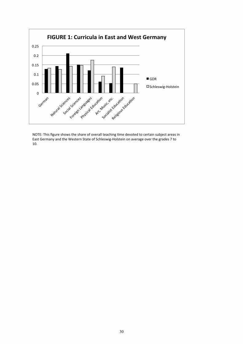
Beyond these two subjects, there were certain differences in the curricula between

East and West Germany, as shown in Figure 1.5 We focus here on grades 7 to 10,

5Curricula in West Germany are determined by the states, but de facto differ littlebetween the states. The information from the GDR comes fromAnweiler (1988), while

6

which are the relevant grades in our empirical analysis. The teaching of German,

mathematics, and social sciences was of similar importance in East and West. How-

ever, GDR schools devoted significantly more time to natural sciences, while FRG

schools devoted more time to teaching of “softer” subjects like foreign languages,

sports, arts and music, and religious education.6 The main foreign language taught

in schools was Russian; it was a compulsory subject in every school in the GDR.

When it comes to teaching styles, there existed important differences between

East and West. In GDR schools, critical thinking was not incentivized, and divergent

opinions were suppressed (Block and Fuchs (1993)). Beyond the creation of a socialist

personality, knowledge transmission was the main official goal of the curricula (Riedel

et al. (1994)). Theorems and theories were never the subject of discussion, but rather

dogmas to be memorized. The national curricula were extremely specific in what

needed to be covered in each week, in part imposing detailed structures of how to

cover certain topics, leaving minimal scope for teacher or student initiatives.

Thus, socialist education in our analysis comprises both the education to a socialist

personality, as well as an education style that did not encourage individual initiative

and independent thinking.7 In basic subjects like mathematics, German language, and

natural sciences, East Germans seem if at all better prepared than West Germans

by schooling, and thus any effect of socialist education is likely not due to lack of

knowledge (which might only arise in the case of English language skills), but rather

due to the education style that minimized critical arguing and individual initiative.

2.3 Allocation of High School Slots and Apprenticeships

Besides academic credentials, political criteria played an important role in the de-

cision of who was allowed to attend the Erweiterte Oberschule. Official selection

criteria were the grades obtained during the 10th grade, as well as a statement about

for the FRG it relates to the state of Schleswig-Holstein (http://www.schulrecht-sh.de/texte/s/stundentafel.htm). We calculate the average teaching hours of eachsubject over grades 7 to 10, taking weighted means over the three school forms ofHauptschule, Realschule and Gymnasium for the West.

6In grades 1 to 4, GDR pupils had much more teaching time devoted to Germanthan FRG pupils, namely around one half of overall teaching hours, as compared toone quarter to one third in the West.

7While the latter is not in itself linked to socialism, it is often associated withnon-democratic regimes, which have incentives to suppress independent thinking andinitiative.

7

the personality of the student. This statement was issued by the director of the

POS ; both the class teacher of the student as well as the Freie Deutsche Jugend, the

de-facto youth group of the government party, were officially involved in the draft-

ing of the statement (Waterkamp (1987)). It was supposed to describe the political

and social involvement of the student, his identification with the GDR - documented

through words and actions - as well as his social background. Children of workers

were more likely to be accepted into the EOS than children coming from an academic

background. Unofficial selection criteria included the intention of a military career,

political position and personal contacts of the parents, as well as a desired career

path that was in line with the official planning numbers (Fischer (1992)). Summariz-

ing, there were important criteria in addition to academic merit which affected the

acceptance into the EOS, and it is thus likely that a significant number of students

who possessed the academic merits were not allowed to attend high school. Similar

criteria were adopted to select the students who were allowed to attend college among

the ones who completed the EOS.

The constitution of the GDR stated that each student had the right (as well as the

obligation) to do an apprenticeship (Köhler (2008)). The number of apprenticeships

in each firm was determined by central planning. Already in the POS, students were

brought in contact with firms which were deemed to be a good fit for them in order

to influence the students’ apprenticeship decision according to the central plan. The

application and allocation process was done centrally, but students could express pref-

erences for a certain apprenticeship in their application. Firms were obliged to offer

apprentices a permanent position at the end of their vocational training (Wehrmeis-

ter (2005)). Similarly to the central planning of apprenticeship positions, the number

of students allowed to start studying a certain subject at the university level was

centrally determined each year. An official survey from the GDR acknowledged that

around one third of all apprentices ended up in an occupation that was not associated

at all with their initial wishes (Anweiler (1988)).

In 1994, Germany passed the so-called “Occupational Rehabilitation Law”.8 This

law established certain monetary rights for students who for political reasons were

not allowed to attend EOS, university, or finish an apprenticeship, and for workers

who were not allowed to work in a job they originally trained for or a similar one.

8Gesetz über den Ausgleich beruflicher Benachteiligungen für Opfer politischer Ver-folgung im Beitrittsgebiet.

8

From 1994 to 2011, 67,400 individuals were granted monetary compensation based

on this law (Bundesregierung (2013)). This is an impressive number, as it certainly

constitutes a lower bound of affected individuals.

Overall, the non-meritocratic access restrictions led to misallocation of students,

and additionally to less incentives for able students to put effort into schooling. The

latter fact was exacerbated by the generally low wage inequality in the East.

2.4 The Situation after Reunification

The educational system in the GDR was transformed very rapidly after the fall of the

Berlin Wall in November 1989. All school reform acts implemented in the states (Län-

der) in East Germany required the elimination of any elements in the curricula which

were directed towards the creation of a socialist personality. Instead, they fostered the

development of an educational system which supports students to act independently

within the framework of the Western society. Individual initiative, motivation, and

creativity became crucial components of the reformed education system. The changes

involved going from strict curricula to more open ones, which specified certain top-

ics to be covered within a semester, but did not lay down weekly plans, and thus

gave more scope to teachers. Implementation of a student-based approach became

a central part of the curricula reforms (Riedel et al. (1994)). A significant share

of teachers, namely approximately 20 percent, were dismissed after reunification.9

These partly targeted dismissals likely accelerated the implementation of the new

curricula and teaching styles, which were also fostered in newly established centers

for in-service training (Block and Fuchs (1993)). Students were allowed to learn other

foreign languages such as English and French. The socialist content of education was

abolished almost immediately, and non-meritocratic access restrictions to the EOS

(and therefore to college) fell at the beginning of 1990 (Fischer (1992)). The voca-

tional training schools were disassociated from government firms and brought under

communal control. The right to freely apply for any apprenticeship was introduced.

Over the period June to September 1990, 18,500 existing apprenticeship contracts

were resolved, of which two thirds would have started in the summer of 1990, 3,500

were in the first year of the apprenticeship, and 2,400 in the second apprentice-

9Web Appendix Section 1 discusses which implications possible temporary inter-ruptions in schooling would have for our results.

9

ship year (Bundesministerium für Bildung und Wissenschaft (1991)).10 This may be

partly because of the students’ choice to attend EOS and subsequently college, but

also because many firms suffered from the economic transition (Wehrmeister (2005)).

Private training programs and public active labor market policies were implemented

in East Germany in order to offer possibilities for retraining and further education.

However, there exists evidence that the success of these programs was limited (see

e.g. Lechner and Wunsch (2009)).

3 Methodology and Data

3.1 Exploiting Cut-Off Birth Dates for School Enrollment

We analyze the effects of socialist education on labor market outcomes based on a

difference-in-differences approach. In the GDR, children turning six on or before May

31 of a given year were per decree enrolled in the first grade by September 1 of the

same year. We define children born June 1 or later as the treated group, and children

born May 31 or before as control group. The difference between respondents in East

Germany in treatment and control group is that, for any given birth cohort still in

school at the time of the fall of the Berlin Wall in November 1989, respondents in the

treatment group were one year less advanced in the socialist education system than

respondents in the control group, and thus acquired one year less of socialist educa-

tion. Treated respondents in the West received instead the same type of education

as non treated respondents.

By comparing individuals born early and late in the year in the East and still

in education at reunification, we compare groups differentially affected by the length

of socialist education; by comparing differences between these groups between East

and West Germany, we control for any potential general effects of entering school at

a slightly older or younger age. The underlying identifying assumption is therefore

that the effect of age at school entry on the dependent variables would be the same in

East and West Germany in absence of the differential exposure to socialist education

10In 1988, 164,000 individuals started an apprenticeship in the East, and in 1989 the

corresponding number was 126,000. Thus, around 1.5% of second year apprentices,

2.8% of first year apprentices, and - under the assumption of the same number ofstarters 1989 and 1990 - 10% of starting apprentices had their contract dissolved in

the four months period June to September 1990 alone.

10

that affects only respondents educated in the East. We show evidence supporting

this assumption in Section 5.1.

We run the following difference-in-differences estimation in order to assess whether

labor market outcomes are affected by socialist education:

\lf = �0 + �1Hdvwlf + �2Wuhdwlf + �3 (Hdvw ∗ Wuhdw)lf + �04 ([)lf + �f + %lw (1)

where \lf is the relevant labor market outcome variable for individual l born in year

f, Hdvw is a dummy variable indicating whether the individual lives in East Germany,

and Wuhdw is a dummy variable being equal to 1 if the individual was born on or after

June 1. We do not have panel data; therefore, we pool several survey years (2005 to

2008). [ is a vector of control variables including a male dummy, a full set of age

dummies, a full set of state of residence dummies, and month of birth, which enters

linearly. When we include state dummies, the East dummy drops out. �f is a full set

of birth year dummies. Standard errors are clustered at the eluwk|hdu-wuhdwphqw-hdvw

level, i.e. at the group level with groups being built based on all possible interactions

of the birth year, treatment, and East dummies.

The coefficient �1 captures the effect of living in the East on labor market out-

comes. The coefficient �2 controls for any potential effects of being enrolled in school

at a slightly older age. The coefficient of main interest is �3, which captures a dif-

ferential effect of being treated for East and West Germans. If being treated leads

to an additional positive labor market effect in East Germany due to experiencing a

shorter GDR education, then �3 should be positive.11

One caveat of the analysis is that we only assign respondents correctly to school

cohorts (and therefore to either treatment or control groups) in the absence of grade

repetition and early or late enrollment into school. Unfortunately, our data set does

not indicate whether an individual ever repeated a grade or whether he/she enrolled

in school a year earlier or later than he/she was supposed to. An incorrect assignment

11We refrain from performing a difference in regression discontinuity exercise (as inCarneiro et al., 2011) for two reasons. First, the cut-off schooling date in the Westwas June 30, rather than May 31. We show a robustness check using this cut-offdate for the West in Section 5. Secondly, early and late enrollment into school makesmeasurement error in allocating individuals into treatment and control groups largestfor individuals born close to the cut-off date. Results using the difference in regressiondiscontinuity approach by Carneiro et al. (2011), and omitting individuals born inthe month of June, are shown in Web Appendix Table W1.

11

of respondents to school cohorts would induce measurement error that may bias our

estimates of �3 upwards under very specific circumstances. In Section 5.1, we conduct

a battery of placebo tests to dismiss the possibility that our results are driven by wrong

assignment to treatment of the respondents in our sample.

3.2 Affected Birth Cohorts

Affected birth cohorts are those still in education at reunification, i.e. born 1971 or

later. We analyze the birth cohorts 1971 to 1977, splitting them up into two separate

cohort groups, namely the cohorts born 1971 to 1973, and those born 1974 to 1977.

We would like to analyze even younger cohorts than the one from 1977, but do not

observe these cohorts yet at the relevant age to investigate labor market outcomes.

When the Berlin Wall fell, individuals in the cohort group 1974 to 1977 were

still in 10th grade or below. For any given cohort in this group, treatment means

having received one year less of GDR education than the control group, and thus

the length of exposure to socialist contents of education and teaching style is the

relevant difference between treatment and control in the cohort group 1974 to 1977.

Our hypothesis is that the longer the exposure to socialist education, the stronger

was the transmission of values that may not be useful in the unified German labor

market and, more generally, in Western societies.

The second relevant cohort group consists of the birth cohorts 1971 to 1973. Con-

sider cohort 1973. While treated individuals were about to complete 10th grade and

therefore free to choose an educational path that was propaedeutic to college educa-

tion or an apprenticeship of their choice in the summer of 1990, individuals in the

control group may have been forced to participate in apprenticeship programs instead

of attending EOS (which granted the university-entrance diploma) in the summer of

1989. Within cohort 1972, individuals in the control group had attended one year

more of the apprenticeship program in November 1989, therefore increasing the cost

of switching to the educational path needed to be able to attend college, or to switch

the apprenticeship subject. On the other hand, as discussed in Section 2.4, they might

have been less likely to be dismissed from an apprenticeship. The treated group in

the cohort 1971 was either in the last year of apprenticeship or in the last year of

EOS and therefore not subject to any restriction in access to college or in the choice

of the subject. By contrast, individuals in the control group had already entered the

12

labor market, had started studying a certain subject at the university, or had started

the compulsory military service for males. Given the high economic uncertainty after

reunification, individuals with a job or an apprenticeship might have feared giving it

up and starting a new career, even if the job was not a good fit for them, affecting

their productivity negatively. While changing the subject at university is theoreti-

cally possible, it involves reapplying. Being stuck in a subject that does not match

the own abilities and interests well might lead to a lower probability of college com-

pletion. The cost of changing the apprenticeship subject, going back to high school

to earn a university-entrance degree, or switching subjects at a university might also

be a purely psychological one based on a resistance to treat sunk costs as such.

Summarizing, for the cohort group 1971 to 1973, the treatment and control groups

differ in how far they have been affected by access restrictions to education. We

conjecture that it was easier to change schooling or apprenticeship for the treatment

group than for the control group, both for practical and psychological reasons.

When we analyze both birth cohort groups separately, we create separate cohort

group dummies for both cohort groups and run the following regression:

\lf = �0 + �1Hdvwlf + �2Wuhdwlf (2)

+�3 (Hdvw ∗ frkruw71−73)lf + �4 (Wuhdw ∗ frkruw71−73)lf+�5 (Hdvw ∗ Wuhdw ∗ frkruw71−73)lf + �6 (Hdvw ∗ Wuhdw ∗ frkruw74−77)lf+�07 ([)lf + �f + %lw

Now �5 and �6 capture any potential additional effect of treatment in the East

compared to the West for the birth cohorts 1971 to 1973 and 1974 to 1977, respec-

tively. �6 should therefore capture the effects of exposure to socialist methods of

education, and �5 the effect of non-meritocratic restrictions in access to high school

and college, as well as restricted apprenticeship choice. We conjecture that differ-

ential exposure to length of socialist education did not matter for the older cohort

group because of the significantly lower teaching time in apprenticeship training, and

because less teaching time was devoted to socialism in both apprenticeship and EOS,

as documented in Section 2.2.

13

3.3 Data and Sample Selection

The German Microcensus is a repeated cross-sectional annual survey on a one percent

random sample of the German population. The main variable that we need for our

analysis is month of birth, which is only available for the years 2005 onwards. Thus,

our main analyses are carried out on the samples 2005 to 2008, in which we define

treatment correctly as being born on or after June 1. We refer to this as “Definition

1” of treatment. In the survey years prior to 2005, month of birth was only reported

as falling either into January to April or May to December,12 thus not coinciding

exactly with our treatment/control definition. We use this less precise definition of

treatment, in which individuals born in May are incorrectly assigned to the treatment

group, when we study the outcomes of older cohorts and therefore need data from

earlier survey rounds in order to observe them at the relevant age.13 We call this

less precise definition of treatment “Definition 2”. We focus on individuals aged 31

to 35. We only start at age 31 in order to capture labor market outcomes at an age

at which individuals are already settled in the labor market. We stop at age 35 such

that the age composition of the different cohorts 1971 to 1977 is not too different in

our sample 2005 to 2008.

The Microcensus provides the current state of residence, but unfortunately does

not report whether an individual resided in the GDR or FRG before 1989. Thus, we

have to work with the current residence as a proxy for residence before 1989, and we

drop respondents from the state of Berlin. In Section 5.4, we address the possibility

that our results are driven by selection into current residence.

We start by analyzing the impact of reunification on the probability of obtaining

a college degree, and then focus on labor market outcomes. The dummy variable

froohjh takes on the value of 1 if the highest educational degree comes from a uni-

versity or an applied university, excluding GDR Idfkvfkxohq. Employment is equal

to 1 if the self-reported employment status is given as employed. Working hours are

hours in a usual work week, of which we take the logarithm. To construct wages, we

have to recur to personal net income, since gross income is not available. Personal net

income is reported in approximately 25 brackets, and we set personal income equal

to the mean point of each bracket in order to calculate net wages by dividing through

12In 2004, the two categories are slightly different: January to March, and April toDecember.13This is the case for Figure 2 and some of the robustness checks.

14

working hours (following the methodology by Pischke and von Wachter (2008)). Last,

surihvvlrqdo is a dummy variable equal to 1 if the respondent is a manager, a profes-

sional, or a technician or associate professional according to the ISCO classification

(major groups 1, 2, and 3 in ISCO88).

We run linear regressions on all dependent variables to ease the interpretation of

the coefficients, but results are robust to running probit specifications if the outcome

variables college, employment, or professional are used. Descriptive statistics of all

variables, also separated by East and West, as well as treatment and control group,

are reported in Table 1.

4 Results

4.1 Results for College Graduation

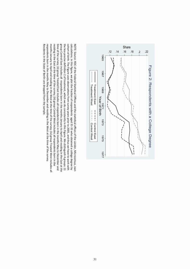
Figure 2 shows the college completion rate by birth cohort for four different groups

of individuals aged 31 to 35, separated by residing in East (thick line) and West

(thin line), and by being born between May and December (treated, solid line) or

January and April (control, dashed line), thus working with the less precise definition

2 of treatment.14 In the West, individuals in the treatment group, and thus having

been enrolled in school at a later age, exhibit slightly higher college completion rates

than individuals in the control group for most birth cohorts. In the East, we observe

the same pattern. Yet, differences become quite large, amounting to around one

percentage point, starting with birth cohort 1971, which is the oldest cohort that may

have been affected by the reorganization of the school and apprenticeship system in

East Germany after reunification. This indicates that treatment might have a larger

effect on college graduation in the East than in the West for the birth cohorts 1971

to 1977. We test the significance of these results, as well as their robustness to the

inclusion of controls, in the following set of regressions.

Panel A of Table 2 shows the results of our main specification, with and without

control variables (gender dummy, age dummies, birth year dummies, state dummies,

and month of birth). The sample used in the regression analysis consists of respon-

dents born between 1971 and 1977; therefore, we can rely on survey years 2005 to

14Since we use birth cohorts from 1965 onwards, we need data from surveys earlierthan 2005. In this figure, we work with the less precise definition 2 of treatment forall cohorts.

15

2008 and use the more precise definition of treatment. The coefficient on East is

negative and highly significant, reflecting lower college graduation rates in the East

than in the West for the birth cohorts 1971 to 1977, as already visible in Figure 2.15

The coefficient of main interest on the interaction term between East and Treatment

is positive and significant, indicating that being enrolled at an older age in the East

and thereby receiving one year less of socialist education increases the probability of

attaining a college degree by 2.1 (column (i)) to 2 (column (ii)) percentage points

more than being enrolled at an older age in the West. Given a college graduation

rate of around 15 percent in the East, this is a very large effect.16 Columns (iii) and

(iv) show that the effect is equally present for both men and women, and is slightly

larger for women than for men.

Panel B of Table 2 shows the results of specification (2) and decomposes the

cohorts used in the analysis into the two cohort groups 1971 to 1973 and 1974 to

1977, first using the full sample (column ii), and then splitting the sample into males

(column iii) and females (column iv). Focusing on the coefficients of interest, the

interaction term between East and Treatment has a significantly positive coefficient

of very similar size for both cohort groups. When the sample is split into females and

males, only the coefficient for females in the older cohort group remains significant.

However, the other three coefficients are of the same order of magnitude, yet with

larger standard errors.17 It is interesting that the large effect of socialist education

on college graduation rates is present and of similar size for the cohort group 1971

to 1973, which was differentially affected by socialist education in terms of non-

meritocratic access restrictions, and the younger cohort group 1974 to 1977, which was

differentially affected in terms of length of socialist education. Even for this younger

group, the large effects are present, indicating strong effects of socialist indoctrination

and socialist teaching styles. The fact that the coefficient is not larger for the older

cohort group than for the younger one implies that differential exposure to length

15Due to the inclusion of state dummies, the East dummy is omitted in columns(ii) to (iv). The coefficient on treatment is insignificant in the specification withoutcontrol variables, and only becomes negative and significant when the control variablemonth of birth is included. This is mostly driven by females, as columns (iii) and (iv)show.16The effect is larger than the one shown in Figure 2. Note that Figure 2 uses the

imprecise definition of treatment (Definition 2) since we need to use survey years priorto 2005, while in the regression we use the precise definition of treatment (Definition1).17p-values vary between 0.11 and 0.19.

16

of socialist education did not matter for the older cohort group, or alternatively

non-meritocratic access restrictions played no role. We conjecture that the former is

true, because of the significantly lower teaching time in apprenticeship training, and

because less teaching time was devoted to socialism in both apprenticeship and EOS,

as documented in Section 2.2. Moreover, the longer-term labor market outcomes show

differential results for both cohort groups. In the web appendix, Panel A of Figure W1

shows coefficients on the relevant interaction terms if we run specification (1) cohort

by cohort. The treatment effect is declining by cohort for the younger cohort group

1974 to 1977, which might indicate that individuals who were in lower grades than 7th

grade at reunification might not experience long-term effects of socialist education on

college attainment anymore. Yet, it could also be random variation, and one would

need to investigate this issue in the future with data on younger generations.

Summarizing the college results, we find significant negative effects of the length

of exposure to socialist contents of education and restricted access to higher education

in the GDR on college completion rates. In Table W2 in the web appendix, we show

that this result is robust to using years of schooling as outcome variable. Additionally,

we report there robust evidence that treated respondents in the East are significantly

less likely to have completed vocational education as the highest educational degree;

thus, treatment induced respondents to switch from completing a vocational education

as highest degree to obtaining a college degree. However, we also find that within

cohorts 1971 to 1973 treated respondents are more likely to not complete any official

vocational degree (although the effect is not significantly different from zero, with a

p-value of .21), an issue we get back to in the next section.

4.2 Results for Longer-Term Labor Market Outcomes

For the four labor market outcomes employment, working hours, wages, and profes-

sional occupation, we directly present results of specification (2), each time presenting

results on the full sample as well as separately for males and females. We discuss the

results for the two cohort groups separately.18

Starting with the older cohort group, born 1971 to 1973, Table 3 shows that being

treated in the East is associated with a significantly lower likelihood of being employed

18Web Appendix Table W3 reports also coefficients on the treatment dummy, andon the interaction term of East and treatment if we do not split the sample into thetwo cohort groups.

17

than in the West, but with significantly higher wages, as well as a higher probability

of being a professional. The employment effect is present for both men and women,

though it is less significant for women than for men, while the effects on wages and

professional status are only present for men. They are however quite large for men,

indicating a 4.1 percent larger effect of treatment on wages in the East than in the

West, and a 5.1 percentage points larger effect on the probability of being employed

as a manager or professional.19 Restrictions in access to education imposed on this

cohort group appear to have had significant long-term effects on the labor market

success of men in terms of making a career. The elimination of non-meritocratic

restrictions in access to college and apprenticeship choice allowed able male students

to acquire the human capital they needed to achieve a better occupational status in

the labor market. Estimates on college returns in Germany typically lie between 20

percent and 40 percent (see Fuchs-Schündeln et al., 2010, and OECD, 2006). If we

accept the estimate of 20 percent coming from a Mincerian regression by the OECD

(2006) as the college wage premium in Germany, and take as the mean estimate of

Table 2 that the effect of treatment on college is about 2 percentage points for both

cohort groups, corresponding to roughly 10 percent of the mean of the college variable,

then we would expect an effect of treatment on wage from college alone of 2 percent

(0.1*0.2=0.02). So these effects are (roughly) in line with an interpretation that for

the older cohort group, there are effects on wages that go beyond college, namely the

general abolishment of non-meritocratic access restrictions leading to better matches.

What is very interesting is the contrasting result on employment: being treated

leads to a lower probability of being employed in the East than in the West. We

conjecture that this effect might come from an increasing variance in labor market

success after reunification. Individuals in the control group were more advanced in

their apprenticeship at reunification and therefore might have been more likely to

finish their vocational education. Individuals who potentially struggle in the labor

market might have been better taken care of in the regulated GDR system than

in the free labor market of the FRG. Therefore, the overall effect of being treated

for this cohort group leads to a larger spread in labor market outcomes: there are

more individuals not being employed, but conditional on being employed treatment

19In Web Appendix Section W2, we provide more disaggregated evidence. Usingthe sample of male respondents in the East, we compare the entire occupationaldistribution of treatment and control groups within birth cohorts 1971-1973, anddiscuss the results.

18

leads to higher wages and a higher probability of achieving a professional status in

the East than in the West. This is consistent with the results on not obtaining any

vocational degree in Web Appendix Table W2, which show weak evidence of a higher

proportion of respondents with the lowest possible educational achievement among

treated individuals within cohorts 1971 to 1973.20

For the younger cohort group born 1974 to 1977, being treated in the East is as-

sociated with a higher probability of being employed, as well as longer working hours,

than being treated in the West.21 Both effects are only present for males. This is in

line with a longer exposure to socialist teaching being detrimental for individual ini-

tiative and motivation. We conjecture that the development of an educational system

after reunification that aimed at encouraging independent thinking and individual

initiative rather than the creation of a socialist personality may have stimulated in-

dividual participation in the labor market, as well as effort in job searches and in the

workplace. The sizes of the coefficients are relevant from an economic point of view

for both employment and working hours: male respondents born between 1974 and

1977 are 2.1 percentage points more likely to be employed, and also increase their

working hours by 1.5 percent when they receive one year less of socialist education,

compared to treated individuals in the West.

Panels B to F of Figure W1 in the Web Appendix present results from regressions

run cohort by cohort for any significant result in Table 3. There are some oscillations

in the size of the coefficient on the interaction term cohort by cohort, but most effects

are economically significant for all cohorts.22 Interestingly, there is no clear decreasing

trend of the effect for the younger cohort group as we find for college attainment.

For females, none of the coefficients on the interaction variables of interest in

20Selection can also play a role here: if the least abled are not employed, then thetreated employed group has on average a higher ability level, which might explainhigher wages and higher chances of having a professional job. Web Appendix Section3 performs a bounding exercise of the potential magnitudes of the possible biases. Wefind as an upper bound that self-selection biases the treatment effect up by 0.008 inthe case of professional status, and 0.012 in the case of wages, i.e. without selectiontreatment would raise the probability of receiving a professional job by 4.3 percentagepoints as a lower bound, and would increase wages by 2.9 percent as a lower bound.21For the younger cohort group born 1974 to 1977, being treated in the East is also

associated with higher wages. This effect, however, is only marginally significant, andit is not robust to several of the robustness checks we present in Table 4 and in WebAppendix Tables W7 and W8.22The two exceptions are the employment effect for cohort 1971 in panel B, and the

employment effect for cohort 1977 in panel E.

19

Table 3 are significant.23 We believe that the lack of significant results for females, in

contrast to males, can be explained by their generally lower labor market attachment.

Women typically experience labor market breaks in their career, and especially at the

beginning of their career, through the arrival of children. These breaks often lead

to new professional orientations. Therefore, any initial effects of restricted access to

education or to the desired apprenticeship might show up less strongly for women

over time than for men. It is interesting that for college graduation, which in the

majority of cases happens before children are born, we see similar effects for females

as for males in terms of the size of the coefficients.

5 Ruling Out Alternative Interpretations of the

Results

In this section, we conduct a series of analyses that rule out alternative explanations

of the results. We conduct these analyses only on the significant results from Tables

2 and 3. For college attainment, we always show results obtained using the whole

sample, given that results were very similar for both cohort groups and for males

and females. Concerning labor market outcomes, for the dependent variables wage

and professional status we show results only for the older cohort group and the male

sample,24 for the dependent variable working hours only for the younger cohort group

and the male sample, while for the employment status we show results for both older

and younger cohort group (but in this last case only using the male sample).

5.1 Are West Germans a Valid Control Group?

An underlying assumption of our exercise is that West Germans are a valid control

group for East Germans. One might be worried about this for different reasons. Since

the school systems in East andWest Germany were very different (e.g. due to tracking

in the West German school system), the effect of enrollment at an earlier age could

differ in East and West. Moreover, as previously discussed, incorrect assignment of

treatment due to grade repetition or early/late enrollment into school may bias the

23All results for females, as well as for males, are robust to controlling for the numberof children. These are shown in Web Appendix Tables W4 to W6.24For wages and professional status, the interaction term of interest is also significant

in the full sample, but these results are entirely driven by the male sample.

20

estimates of our coefficients of interest. In particular, this may be the case if the

share of respondents who repeat their grade is systematically different in treatment

and control group, and such a difference depends on whether we consider the sample

of East or West respondents. Last, one general worry about the results could be that

they might capture differences in age trends between East and West residents, since

treatment and control individuals are slightly different in terms of age.

Yet, any of these potential biases should show up also for older cohorts born

before 1971. Thus, to rule out these alternative interpretations of the results and

biases, we run regressions on placebo cohort groups, namely cohorts born between

1961 and 1970.25 All respondents born 1970 or before had already completed primary

and secondary education when the Berlin Wall fell, and were thus not differentially

affected by socialist education, but would face the same biases driven by differential

age trends, early/late enrollment or grade repetition.26

Figure 3 presents the results for different placebo cohort groups, starting from the

cohort group 1961 to 1970, 1962 to 1970, up to 1968 to 1970. The figure shows the

coefficients on the interaction variable of interest between East and Treat. In Panel

A, college attainment is the dependent variable, while Panels B to F focus on the

labor market outcomes. For comparison, the panels also show the coefficients for our

two relevant cohort groups 1971 to 1973 and 1974 to 1977 from Tables 2 and 3. None

of the coefficients of interest on the interaction of East and Treatment are significant

for the placebo cohort groups, and indeed most are very close to zero. Thus, we are

quite sure that we indeed capture effects of socialist education, rather than general

East or West German trends or biases that should also have been present for cohorts

1970 and older.

5.2 General Exposure to Socialist Regime

We next address the possibility that our results are driven by general exposure to

a socialist regime and lifestyle, rather than specifically by socialist education. Due

25For these robustness checks, we have to use the survey years from 2004 and beforein order to observe these cohorts at the same age 31 to 35 as the individuals in ourbaseline analyses. Thus, we have to recur to the second, less precise definition oftreatment (being born on or after May 1). In Web Appendix Table W7, we show thatour main results are robust to using this less precise definition of treatment.26An underlying assumption is that East-West differences in regular enrollment and

grade repetition did not change significantly for cohorts born before or after 1971.

21

to their younger age, respondents in the treatment group have been less exposed to

socialist culture in general if they come from the East.

The exercises performed in the previous subsection should already be enough to

rule out the possibility that length of exposure to socialist culture in general matters,

unless we believe that exposure to socialist culture should have a stronger impact at

a younger age and in particular at the age when cohorts 1971 to 1977 experienced

reunification. Still, we perform an additional robustness check, in which we restrict

the sample to respondents born between February and September. Thereby, we are

comparing individuals whose age differences are very small, and therefore it is less

likely that results are driven by different exposure to socialist culture in general.

Results for college graduation are presented in Panel A of column (i) of Table 4,

while Panels B and C present results using labor market outcome variables for the

older and younger cohort group, respectively. As expected, all coefficients of interest

remain of the same sign as in the baseline results and significant.27

5.3 Year of Labor Market Entrance

Since individuals in the treatment group enter school one year later, they also enter

the labor market one year later than individuals in the control group from the same

birth cohort. Given that the East German labor market was in a recession after reuni-

fication, this might have mattered. In fact, unemployment rates generally increased

in the first years after reunification (see Figure W4 in the web appendix). In order

to control for labor market conditions after reunification, we collect information on

the unemployment rates of the total and male population in East and West Germany

from 1991 onwards from the Federal Employment Agency. We then generate a vari-

able “unemployment rate in the year of labor market entrance”, which associates to

each individual the unemployment rate observed in East or West Germany (depend-

ing on the current residence) 20 years after the individual’s birth year for individuals

in the control group, and 21 years for individuals in the treatment group, who enter

the labor market one summer later. Based on data from the German Socio-Economic

Panel, the average age at the first job for individuals fitting our sample criteria is 20.7

27Web Appendix TableW8 shows results from a placebo treatment, in which we con-sider only individuals born between July and December, defining those born betweenOctober and December as the placebo treatment group, and those born betweenJuly and September as the placebo control group. None of the placebo treatmentcoefficients is significant.

22

in the East and 20.6 in the West for individuals in the treatment group, and 20.2 or

20.1, respectively, for individuals in the control group.

We add this newly created variable “unemployment rate in the year of labor

market entrance”, either referring to the total or the male population, as a control to

the baseline specifications in columns (ii) and (iii) of Table 4. Column (iv) instead

adds linear trends in the year of labor market entrance; this way, we do not have to

make any assumptions on when exactly the individuals enter the labor market, but

only that each school cohort enters at the same point in time. All results are robust

to adding these additional control variables.28

5.4 East-West Migration

One unfortunate feature of the German Microcensus is that it provides information

only on the current residence of the respondents, but not on their residence before

reunification. Therefore, when generating the variable “East”, we are implicitly as-

suming that respondents currently residing in the East (West) also received their

education in the East (West). This assumption needs to be carefully discussed given

that migration flows from East to West Germany have been substantial (see e.g. Hunt

(2006) and Fuchs-Schündeln and Schündeln (2009)).29 In particular, this assumption

may bias the coefficient of the interaction term between the variables “East” and

“Treatment” upwards, if the most talented and hard working respondents in the

treatment group were less likely to migrate from the East towards the West than the

corresponding most talented and hard working respondents in the control group.

While the Microcensus does not provide a full migration history of each respon-

dent, it reports the state of residence in the current and the previous year (except for

28In Table W9 in the Web Appendix, we show a battery of additional robust-ness checks controlling for unemployment rates in the year of labor market entrance,namely including quadratic terms in the total or male unemployment rate, controllingfor the youth unemployment rate (in levels and squared) or state-specific unemploy-ment rates (again in levels and squared). Last, we include state-specific linear trends.The youth unemployment rate is only available from 1993 on, such that we can onlyinclude individuals who entered the labor market in 1993 or later, which restricts thesample to the cohort group 1974-1977.29A quick back-of-the-envelope calculation reveals that as an upper bound, East

Germans constitute 4.7 percent of the West sample. This calculation is based oncumulative East-West flows from 1989 to 2006, and assumes that 20% of East-Westmigrants return to the East. The rate of East German return migrants is calculatedto be 20% based on German Socio-Economic Panel data by Fuchs-Schündeln andSchündeln (2009), who indicate that this number is a lower bound.

23

the survey years 2004, 2006, and 2007). Using the sample of all respondents belonging

to cohorts 1971 to 1977 who resided in East Germany 12 months prior to the interview

and all surveys from 1991 onwards, this allows us to check whether respondents in the

treatment group were more likely to migrate in the next year than respondents in the

control group. The results are shown in Web Appendix Table W10.30 Both with and

without including control variables, the coefficient on the treatment variable is very

close to zero and far from being significantly different from zero, suggesting that it is

highly unlikely that patterns of migration have been somehow influenced by the re-

organization of the educational system after 1989. Since migration to West Germany

was not negligible, however, we need to stress that our findings are only restricted to

the fraction of East Germans who did not move to the West after reunification. To

achieve a definite answer to the question whether migration explains the results, we

would need to be able to analyze the migration pattern not only based on treatment,

but also based on the ability of the individuals interacted with treatment.

5.5 Robustness Checks

In TableW7 in theWeb Appendix, we also show that results are robust to (i) including

data from 2004 and before, working with the less precise Definition 2 of treatment;

(ii) defining treatment in the West as being born between July and December, given

that the relevant cut-off date for schooling was typically June 30 in the West in the

1980s, not May 31 as in the GDR; (iii) dropping respondents from May, June, or

July, for whom wrong assignment to treatment or control is most likely in case of

early or late enrollment; and (iv) redefining the college variable by assigning college

status also to an individual whose highest educational degree is from a Fachschule.

All results are robust.30To use the early survey years, we have to rely on the less precise definition 2 of

treatment. Web Appendix Table W11 shows the results year by year: in two years,namely 1993 and 1997, the treated were significantly more likely to migrate West,while in one year, namely 1992, they were significantly less likely to do that. Yet,there is no clear trend in migration of treatment vs. control group.

24

6 Conclusion

The event of German reunification and the rapid transformation of the educational

system in East Germany towards a Western model provide a unique setting to assess

how political regimes influence individual lives through education. We identify two

possible channels: authoritarian, and in particular socialist, forms of government

often (i) adopt non-meritocratic criteria to select students and grant access to higher

education, and impose restrictions on occupational choice based on central planning,

and (ii) shape the contents of curricula to indoctrinate pupils and preserve consensus

towards the regime in power, with a teaching style that does not encourage critical

discussion. We find that the removal of both these features of the socialist education

system increases the likelihood of obtaining a college degree of respondents resident

in East Germany, once the transition towards a capitalist society is completed.

Interestingly, the two channels have quite different effects on labor market out-

comes. Elimination of restrictions to access to college and restrictions put on occu-

pational choice allows skilled students to acquire higher human capital and therefore

better paid jobs. At the same time, we find some suggestive evidence that less able

students face a higher likelihood of being non-employed. Thus, the elimination of

these restrictions might have increased the variance of labor market outcomes. The

abolishment of socialist teaching instead has different consequences. The transition

to a system where individual initiative is encouraged leads to higher participation in

the labor market and higher effort in the workplace, expressed in a larger number of

working hours. The effects that we find in the labor market are, however, limited to

the male sample.

One caveat of our analysis is that it is carried out against the background of a

depressed labor market in East Germany right after reunification. The high unem-

ployment rates might have made it more difficult for young people to switch education

and adjust their occupational choice after the fall of the Berlin Wall, and therefore

the effects of restricted occupational choice and non-meritocratic restrictions in access

to college might have been larger than in settings with a booming labor market. Yet,

this concerns the quantities of the results, not the qualitative results.

25

References

[1] Acemoglu, Daron, Simon Johnson, and James Robinson (2001). “The Colonial

Origins of Comparative Development: An Empirical Investigation”, American

Economic Review, 91(5): 1369-1401.

[2] Acemoglu, Daron, Simon Johnson, and James Robinson (2005). “Institutions as

the Fundamental Cause of Long-Run Growth”, in: Aghion, Philippe, and Steven

Durlauf (eds.): Handbook of Economic Growth, Elsevier, 385-472.

[3] Algan, Yann, Pierre Cahuc, and Andrei Shleifer (2013). “Teaching Practices and

Social Capital”, American Economic Journal: Applied Economics, 5(3): 189-210.

[4] Alesina, Alberto, and Nicola Fuchs-Schündeln (2007). “Goodbye Lenin (or Not?):

The Effect of Communism on People’s Preferences”, American Economic Review,

97(4): 1507-1528.

[5] Angrist, Joshua D., and Alan B. Krueger (1991). “Does Compulsory School

Attendance Affect Schooling and Earnings”, Quarterly Journal of Economics,

106(4): 979-1014.

[6] Angrist, Joshua D., and Victor Lavy (1997). “The Effect of a Change in Lan-

guage of Instruction on the Returns to Schooling in Morocco”, Journal of Labor

Economics, 15(1): 48-76.

[7] Anweiler, Oskar (1988). “Schulpolitik und Schulsystem in der DDR”,

Leske+Budrich.

[8] Barro, Robert J. (1999). “Determinants of Democracy”, Journal of Political

Economy, 107(S6): S158-S183.

[9] Black, Sandra E., Paul J. Devereux, and Kjell G. Salvanes (2011). “Too Young

to Leave the Nest? The Effects of School Starting Age”, Review of Economics

and Statistics, 93: 455-467.

[10] Block, Klaus-D., and Hans-W. Fuchs (1993). “The Eastern German Education

System in Transition”, in: Reuter, Lutz R., and Gerhard Strunk (eds.): Beiträge

aus dem Fachbereich Pädagogik, Universität der Bundeswehr Hamburg.

26

[11] Bowles, Samuel, and Herbert Gintis (1976). “Schooling in Capitalist America:

Educational Reform and the Contradictions of Economic Life”, New York: Basic

Books.

[12] Brunello, Giorgio, Elena Crivellaro, and Lorenzo Rocco (2012). “Lost in Transi-

tion? The Returns to Education Acquired under Communism 15 Years after the

Fall of the Berlin Wall”, Economics of Transition, 20(4): 637-676.

[13] Bundesministerium für Bildung undWissenschaft (1991). “Berufsbildungsbericht

1991”, Schriftenreihe Grundlagen und Perspektiven für Bildung und Wis-

senschaft, 28.

[14] Bundesregierung (2013): “Bericht der Bundesregierung

zum Stand der Aufarbeitung der SED-Diktatur”,

http://www.bundesregierung.de/Content/DE/_Anlagen/BKM/2013-01-08-

bericht-aufarbeitung-sed-diktatur.pdf?__blob=publicationFile.

[15] Cantoni, Davide, and Noam Yuchtman (2013). “The Political Economy of Edu-

cational Content and Development: Lessons from History”, Journal of Develop-

ment Economics, 104: 233-244.

[16] Cantoni, Davide, Yuyu Chen, David Yufan Yang, Noam Yuchtman, and Y. Jane

Zhang (2015). “Curriculum and Ideology”, Journal of Political Economy, forth-

coming.

[17] Carneiro, Pedro, Katrine V. Løken, and Kjell G. Salvanes (2015). “A Flying

Start? Maternity Leave Benefits and Long Run Outcomes of Children”, Journal

of Political Economy, 123(2): 365-412.

[18] Chetty, Raj, John N. Friedman, and Jonah E. Rockoff (2014). “Measuring the

Impact of Teachers II: Teacher Value-Added and Student Outcomes in Adult-

hood”, American Economic Review, 104(9): 2633-2679.

[19] Clots-Figueras, Irma, and Paolo Masella (2013). “Education, Language and Iden-

tity”, Economic Journal, 123(570): F332-F357.

[20] Fischer, Andreas (1992). “Das Bildungssystem der DDR: Entwicklung, Umbruch

und Neugestaltung seit 1989”, Darmstadt: Wissenschaftliche Buchgesellschaft.

27

[21] Fuchs-Schündeln, Nicola, Dirk Krueger, andMathias Sommer (2010). “Inequality

Trends for Germany in the Last Two Decades: A Tale of Two Countries”, Review

of Economic Dynamics, 31(1): 103-132.

[22] Fuchs-Schündeln, Nicola, and Matthias Schündeln (2009). “Who Stays, Who

Goes, Who Returns? East-West Migration within Germany since Reunification”,

Economics of Transition, 17(4): 703-738.

[23] Glaeser, Edward L., Giacomo Ponzetto, and Andrei Shleifer (2007).“Why Does

Democracy Need Education?”, Journal of Economic Growth, 12(2): 77-99.

[24] Guriev, Sergei, and Ekaterina Zhuravskaya (2009). “(Un)Happiness in Transi-

tion”, Journal of Economic Perspectives, 23(2): 143-168.

[25] Hunt, Jennifer (2006): “Staunching Emigration from East Germany: Age and

the Determinants of Migration”, Journal of the European Economic Association,

4(5): 1014-1037.

[26] Hoffmann, Florian, and Philip Oreopoulos (2009). “Professor Qualities and Stu-

dent Achievement”, Review of Economics and Statistics, 91(1): 83-92.

[27] Köhler, Helmut (2008). “Datenhandbuch zur deutschen Bildungsgeschichte Band

IX: Schulen und Hochschulen in der Deutschen Demokratischen Republik 1949-

1989”, Göttingen: Vandenhoeck & Ruprecht.

[28] Krueger, Alan B., and Mikael Lindahl (2001). “Education for Growth: Why and

for Whom?”, Journal of Economic Literature, 39(4): 1101-1136.

[29] Lechner, Michael, and Conny Wunsch (2009). “Active Labor Market Policy in

East Germany”, Economics of Transition, 17(4): 661-702.

[30] Münich, Daniel, Jan Svejnar, and Katherine Terrell (2005). “Returns to Human

Capital under the Communist Wage Grid and during the Transition to a Market

Economy”, Review of Economics and Statistics, 87(1): 100-123.

[31] North, Douglass C. (1981). “Structure and Change in Economic History”. New

York: Norton & Co.

28

[32] Organisation for Economic Co-operation and Development (2006). The Policy

Determinants of Investment in Tertiary Education: Data and Methodologcial

Issues.

[33] Orazem, Peter, and Milan Vodopivec (1997). “Value of Human Capital in Tran-

sition to Market: Evidence from Slovenia”, European Economic Review, 41(3-5):

893-903.

[34] Pischke, Jörn-Steffen, and Till vonWachter (2008). “Zero Returns to Compulsory

Schooling in Germany: Evidence and Interpretation”, Review of Economics and

Statistics, 90(3): 592-598.

[35] Puhani, Patrick A., and Andrea M. Weber (2007). “Does the Early Bird Catch

the Worm?: Instrumental Variable Estimates of Educational Effects of Age of

School Entry in Germany”, Empirical Economics, 32: 359-386.

[36] Riedel, Klaus, Martin Griwatz, Hans Leutert, and Jürgen Westphal (1994).

“Schule im Vereinigungsprozess. Probleme und Erfahrungen aus Lehrer- und

Schülerperspektive”, Frankfurt am Main: Peter Lang.

[37] Waterkamp, Dietmar (1987). “Handbuch zum Bildungswesen der DDR”, Berlin:

Spitz.

[38] Wehrmeister, Frank (2005). “Betriebsberufsschulen in der ehemaligen DDR”,

in: Illerhaus, K. (ed.): Koordinierung der Berufsausbildung in der Kultusmin-

isterkonferenz. Festschrift anlässlich der 250. Sitzung des Unterausschusses für

Berufliche Bildung der Ständigen Konferenz der Kultusminister der Länder in

der Bundesrepublik, 70-85, Bonn.

29

0"

0.05"

0.1"

0.15"

0.2"

0.25"

FIGURE'1:'Curricula'in'East'and'West'Germany'

GDR"

Schleswig3Holstein"

NOTE:"This"figure"shows"the"share"of"overall"teaching"Cme"devoted"to"certain"subject"areas"in"East"Germany"and"the"Western"State"of"Schleswig3Holstein"on"average"over"the"grades"7"to"10.""

30

NOTE:&Source:&R

DC&of&th

e&Federal&Sta7s7cal&O

ffices&and&th

e&sta7s7cal&offices&of&th

e&Länder,&M

icrocensus,&own&

calcula7ons.&In

&this&figure,&w

e&plot&th

e&fra

c7on&of&re

spondents&&aged&31H35&who&obtained&a&college&degree&by&

cohort&o

f&birth

.&The&Figure&uses&observa7ons&fro

m&survey&years&prio

r&to&2005,&and&th

us&we&have&to

&work&with

&

the&less&precise&defini7on&2&of&tre

atm

ent,&w

hich&we&do&consistently

&in&th

is&Figure.&W

e&dis7nguish&4&groups:&(i)&

group&Contro

l&East&in

cludes&all&&re

spondents&born&in&th

e&m

onths&Ja

nuary&to

&April&a

nd&re

siding&in&th

e&East&a

t&the&

7me&of&th

e&survey;&(ii)&g

roup&Treated&East&in

cludes&all&re

spondents&born&in&th

e&m

onths&M

ay&to

&December&a

nd&

residing&in&th

e&East&a

t&the&7me&of&th

e&survey;&(iii)&g

roup&Contro

l&West&in

cludes&all&re

spondents&born&in&th

e&

months&Ja

nuary&to

&April&a

nd&re

siding&in&th

e&W

est&a

t&the&7me&of&th

e&survey;&(iv

)&group&Treated&W

est&in

cludes&all&

respondents&born&in&th

e&m

onths&M

ay&to

&December&a

nd&re

siding&in&th

e&W

est&a

t&the&7me&of&th

e&survey.&

Residents&in&th

e&State&of&B

erlin

&are&dropped&fro

m&th

e&sample.&

&

.12 .14 .16 .18 .2 .22Share

196

51

96

71

96

91

97

11

97

31

97

51

97

7Y

ea

r of B

irth

Tre

atm

ent E

ast

Con

trol E

ast

Tre

atm

ent W

est

Con

trol W

est

Fig

ure

2: R

esp

on

de

nts w

ith a

Co

lleg

e D

egre

e

31

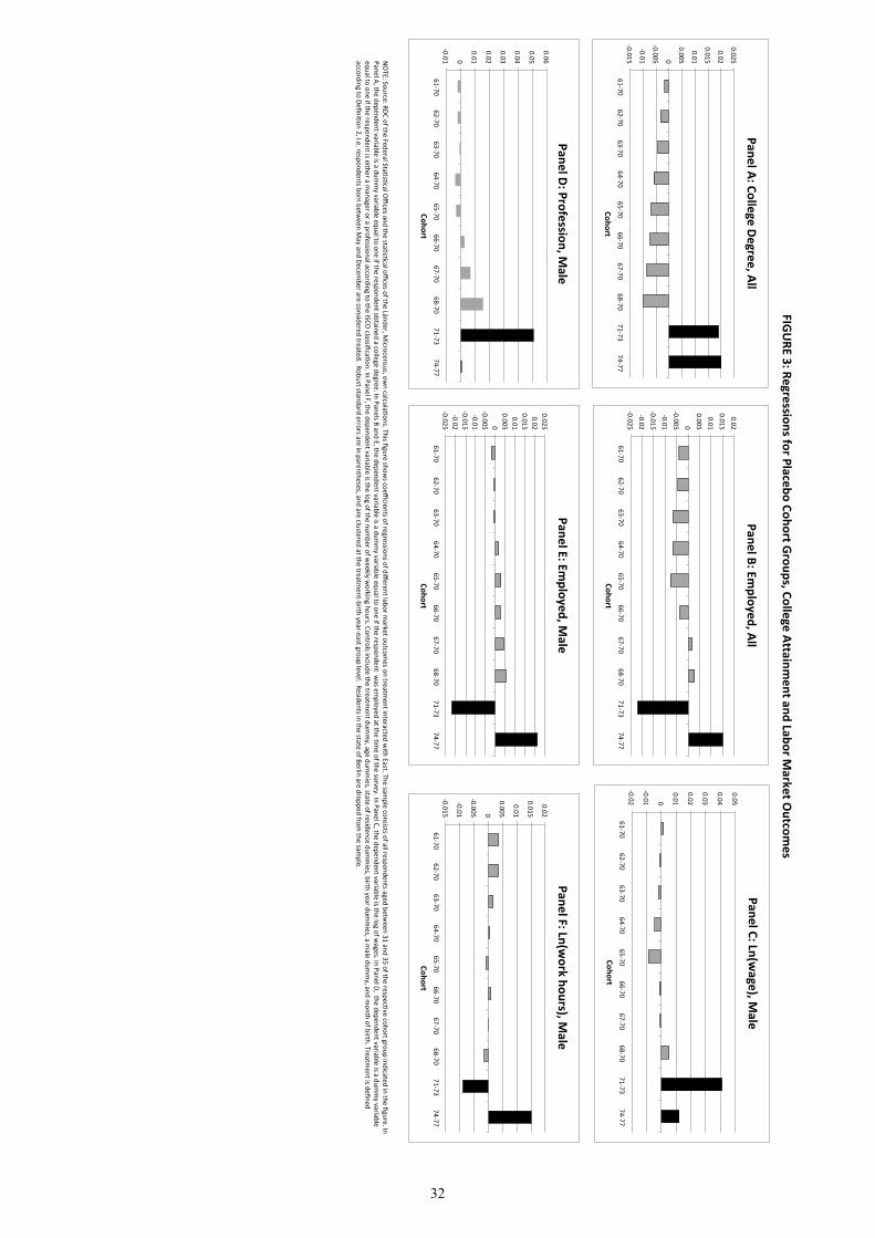
FIGURE'3:'Regressions'for'Placebo'Cohort'Groups,'College'Attainm

ent'and'Labor'Market'O

utcomes

!0.02%

!0.01%

0%

0.01%

0.02%

0.03%

0.04%

0.05%

61!70% 62!70%

63!70% 64!70% 65!70%

66!70% 67!70%

68!70%

71!73% 74!77%

Cohort'

Panel'C:'Ln(wage),'M

ale'

!0.025%

!0.02%

!0.015%

!0.01%

!0.005%

0%

0.005%

0.01%

0.015%

0.02%

0.025%

61!70% 62!70% 63!70% 64!70% 65!70% 66!70% 67!70% 68!70% 71!73% 74!77%

Cohort'

Panel'E:'Employed,'M

ale'

!0.015%

!0.01%

!0.005%

0%

0.005%

0.01%

0.015%

0.02%

61!70% 62!70% 63!70% 64!70% 65!70% 66!70% 67!70% 68!70% 71!73% 74!77%

Cohort'

Panel'F:'Ln(work'hours),'M

ale'

!0.01%

0%

0.01%

0.02%

0.03%

0.04%

0.05%

0.06%

61!70% 62!70% 63!70% 64!70% 65!70% 66!70% 67!70% 68!70% 71!73% 74!77%

Cohort'

Panel'D:'Profession,'Male'

NOTE:%So

urce

:%RDC%of%th

e%Fe

deral%Sta

BsBcal%O

ffices%a

nd%th

e%sta

BsBcal%offices%o

f%the%Lä

nder,%M

icrocensus,%o

wn%ca

lculaBons.%T

his%fi

gure%sh

ows%co

efficie

nts%o

f%regressio

ns%o

f%different%la

bor%m

arke

t%outco

mes%o

n%tre

atm

ent%in

teracte

d%with

%East.%T

he%sa

mple%co

nsists%o

f%all%re

spondents%a

ged%betw

een%31%and%35%of%th

e%re

specBve%co

hort%g

roup%indica

ted%in%th

e%figure.%In

%

Panel%A

,%the%dependent%va

riable%is%a

%dummy%va

riable%equal%to

%one%if%th

e%re

spondent%o

btained%a%co

llege%degree.%In

%Panels%B

%and%E,%th

e%dependent%va

riable%is%a

%dummy%va

riable%equal%to

%one%if%th

e%re

spondent%%w

as%e

mployed%at%th

e%Bme%of%th

e%su

rvey.%In

%Panel%C,%th

e%dependent%va

riable%is%th

e%log%of%w

ages.%In

%Panel%D

,%%the%dependent%va

riable%is%a

%dummy%va

riable%

equal%to

%one%if%th

e%re

spondent%is%e

ither%a

%manager%o

r%a%professio

nal%acco

rding%to

%the%ISC

O%cla

ssificaBon.%In

%Panel%F,%th

e%dependent%va

riable%is%th

e%log%of%th

e%number%o

f%weekly%w

orkin

g%hours.%C

ontro

ls%inclu

de%th

e%tre

atm

ent%d

ummy,%a

ge%dummies,%sta

te%of%re

sidence%dummies,%b

irth%ye

ar%d

ummies,%a

%male%dummy,%a

nd%m

onth%of%b

irth.%Treatm

ent%is%d

efined%

acco

rding%to

%DefiniBon%2,%i.e

.%respondents%b

orn%betw

een%M

ay%a

nd%December%a

re%co

nsid

ered%tre

ated.%%R

obust%sta

ndard%erro

rs%are%in%parentheses,%a

nd%are%clu

stered%at%th

e%tre

atm

ent!b

irth%ye

ar!e

ast%g

roup%level.%%R

esid

ents%in

%the%sta

te%of%B

erlin

%are%dropped%fro

m%th

e%sa

mple.%%

!0.025%

!0.02%

!0.015%

!0.01%

!0.005%

0%

0.005%

0.01%

0.015%

0.02%

61!70% 62!70% 63!70% 64!70% 65!70% 66!70% 67!70% 68!70% 71!73% 74!77%

Cohort'

Panel'B:'Employed,'All'

!0.015%

!0.01%

!0.005%

0%

0.005%

0.01%

0.015%

0.02%

0.025%

61!70% 62!70% 63!70% 64!70% 65!70% 66!70% 67!70% 68!70% 71!73% 74!77%

Cohort'

Panel'A:'College'Degree,'All'

32

TreatedControl

TreatedControl

mean/percent

mean/percent

mean/percent

mean/percent

mean/percent

(i)(ii)

(iii)(iv)

(v)

College0.196

0.1690.149

0.1960.196

Employed

0.7400.740

0.7550.738

0.749

LnA(workAhours)

3.4973.566

3.5683.487

3.479(0.494)

(0.380)(0.379)

(0.510)(0.520)

LnA(wage)

2.1641.970

1.9702.190

2.210(0.563)

(0.527)(0.526)

(0.565)(0.564)

Professional0.463

0.4230.404

0.4670.462

Male

0.4950.515

0.5150.488

0.495

Age33.0

32.933.0

32.933.0

(1.381)(1.398)

(1.385)(1.378)

(1.380)East

0.153

TreatedA(DefinitionA1)0.561

EastWest

TABLE&1:&Sample&Characteristics

NOTE:ASource:ARDCAofAtheAFederalAStaTsTcalAO

fficesAandAtheAstaTsTcalAoffi

cesAofAtheALänder,AMicrocensusA2005X2008,Aow

nAcalculaTons.ATheAsampleAincludesA

onlyArespondentsAagedAbetweenA31AandA35AandAbornAbetw

eenA1971AandA1977.AWhenAtheAvariableA"East"AisAused,Aw

eAdropArespondentsAfromAtheAstateAofA

Berlin.ATheAsamplesAinAcolum

nsA(ii)AandA(iv)AincludeAallArespondentsAbornAbetweenAJuneAandADecem

ber.ATheAsamplesAinAcolum

nsA(iii)AandA(v)AincludeAallArespondentsAbornAbetw

eenAJanuaryAandAMay.AI.e.,Atreatm

entArefersAtoAourA"DefiniTonA1"AofAtreatment.AStandardAdeviaTonsAareAinAparentheses.A

33

Dependent'variable:''

Panel'A:'cohorts'71777

''''''''''''''''''''(i)

(ii)(iii)

(iv)males

females

East'7.047***(.008)

Treated'(Def.'1)

7.00047.013**

7.0077.018**

(.005)(0.005)

(0.007)(.008)

East*Treated'(Def.'1)

.021*.020***

.018*.022**

(.011)(.007)

(.009)(.010)

Controlsx

xx

Observations''''''''

139605139605

6909070515

Panel'B:'cohorts'71773'vs.'74777''''''''''''''''''''

(ii)(iii)

(iv)males

females

East*Treat*cohort71773.019*

.015.022**

(.010)(.011)

(.010)East*Treat*cohort74777

.020**.020

.022(.010)

(.012)(.015)

Controlsx

xx

Observations''''''''

13960569090

70515

College&DegreeTABLE&2:&M

ain&Results

NOTE:'Source:'RD

C'of'the'Federal'StaQsQcal'O

ffices'and'the'staQ

sQcal'offi

ces'of'the'Länder,'Microcensus'200572008,'ow

n'calculaQons.'The'dependent'

variable'is'a'dummy'variable'equal'to'one'if'the'respondent'obtained'a'college'degree.'Treatm

ent'is'defined'according'to'DefiniQ

on'1,'that'is'respondents'born'betw

een'June'and'Decem

ber'are'considered'treated.'The'variable'East'is'dropped'from'the'specificaQ

ons'in'columns'(ii)'to'(iv)'since'state'of'residence'

dummies'are'added.'''Controls'in'colum

ns'(ii)'to'(iv)'include'age'dummies,'state'of'residence'dum

mies,'birth'year'dum

mies,'a'm

ale'dummy,'and'm

onth'of'birth.''Robust'standard'errors'are'in'parentheses,'and'are'clustered'at'the'treatm

ent7birth'year7east'group'level.'The'sample'consists'of'all'respondents'

aged'between'31'and'35'and'born'betw

een'1971'and'1977.'Residents'in'the'state'of'Berlin'are'dropped'from'the'sam

ple.''In'Panel'B,'we'generate'2'

dummies:'one'that'is'equal'to'one'if'the'respondent'w

as'born'between'1971'and'1973,'the'other'that'is'equal'to'one'if'the'respondent'w

as'born'between'

1974'and'1977.'We'then'include'in'the'regression'interacQ

ons'between'each'of'the'tw

o'dummies'and'the'variables'East'and'Treat,'that'is'

East*cohort71773,'East*cohort74777,'Treat*cohort71773,'Treat*cohort74777.'*significant'at'the'10%'level,'**'significant'at'the'5%

'level,'***'significant'at'the'1%

'level.'''

34

Dependent'variable:'''

''''''''''''''''''''(i)

(ii)(iii)

(iv)(v)

(vi)(vii)

(viii)(ix)

(x)(xi)

(xii)all

males

females

allmales

females

allmales

females

allmales

females

East*Treat*cohort71=73'=.022**

'=.022*=.021

'=.019=.009

'=.035'.026***

.041***.006

'.026**.051***

'=.004(.009)

(.012)(0.014)

(.012)(.008)

(.028)(.008)

(.011)(.016)

(.011)(.009)

(.014)East*Treat*cohort74=77

0.015.021***

.009=.005

.015***'=.027

.018*'.012

.022=.001

.002'=.002

(.010)(.004)

(.019)(.009)

(.005)(.019)

(.010)(.010)

(.014)(.007)

(.015)(.022)

Controlsx

xx

xx

xx

xx

xx

xObservations''''''''

13960569090

70515113086

6083852248

10649657487

49009111995

6014051855

Professional+Ln+(w

age)Ln+(w

ork+hours)Em

ployedTABLE+3:+Labor+M

arket+Outcom

es

NOTE:''Source:'RDC'of'the'Federal'StaNsNcal'O

ffices'and'the'staNsNcal'offi

ces'of'the'Länder,'Microcensus'2005=2008,'ow

n'calculaNons.'In'Columns'(i)=(iii)'the'dependent'variable'is'a'

dummy'variable'equal'to'one'if'the'respondent''w

as'employed'at'the'Nm

e'of'the'survey.'In'Columns'(iv)=(vi)'the'dependent'variable'is'the'log'of'the'num

ber'of'weekly'w

orking'hours.'In'Colum

ns'(vii)=(ix)'the'dependent'variable'is'the'log'of'wages'(see'the'text'for'a''detailed'explanaNon'of'how

'wages'are'calculated).'In'Colum

ns'(x)'to'(xii)'the'dependent'variable'is'a'dum

my'variable'equal'to'one'if'the'respondent'is'either'a'm

anager'or'a'professional'according'to'the'ISCO'classificaNon.'W

e'generate'2'dummies:'one'that'is'equal'to'one'if'the'

respondent'was'born'betw

een'1971'and'1973,'the'other'that'is'equal'to'one'if'the'respondent'was'born'betw

een'1974'and'1977.'We'then'include'in'the'regression'interacNons'

between'each'of'the'tw

o'dummies'and'the'variables'East'and'Treat,'that'is'East*cohort71=73,'East*cohort74=77,'Treat*cohort71=73,'Treat*cohort74=77.'Controls''include'age'

dummies,'state'of'residence'dum

mies,'birth'year'dum

mies,'a'm

ale'dummy,'and'm

onth'of'birth.'Treatment'is'defined'according'to'DefiniNon'1,'that'is'respondents'born'betw

een'June'and'Decem

ber'are'considered'treated.'Robust'standard'errors'are'in'parentheses,'and'are'clustered'at'the'treatment=birth'year=east'group'level.''The'sam

ple'consists'of'all'respondents''aged'betw

een'31'and'35'and'born'between'1971'and'1977.'Residents'in'the'state'of'Berlin'are'dropped'from

'the'sample.'*significant'at'the'10%

'level,'**'significant'at'the'5%

'level,'***'significant'at'the'1%'level.'''

35

Panel&A&:&&East*Treat&&&&&&&&&&&&&&&&&&&&

sample

(i)(ii)

(iii)(iv)

Feb7SepUR

male&U

Rmarket&entr.&trends

Collegeall

.026**.020***

.020***.020***

(.012)(.007)

(.006)(.007)

Panel&B&:&&East*Treat*cohort71773&&&&&&&&&&&&&&&&&&&&

(i)(ii)

(iii)(iv)

Employed

all7.016**

&7.020**7.023**

7.021**(.007)

(.009)(.009)

(.010)Ln&(w

age)male

.029**.036***

.044***.041***

(.012)(.008)

(.011)(.011)

Professionalmale

.045***.045***

.056***.051***

(.012)(.009)

(.009)(.009)

&&

Panel&B:&East*Treat*cohort74777&!!!!!!!!!!!!!!!!!!!!

(i)(ii)

(iii)(iv)

Employed

male

.043***.022***

.023***.021***

(.013)(.004)

(.005)(.004)

Ln&(Working&hours)

male

.013*.015***

.014***.015***

(.007)(.004)

(.004)(.005)

TABLE!4:!Further!Analyses

NOTE:&Source:&RDC&of&the&Federal&StaWsWcal&O

ffices&and&the&staWsWcal&offi

ces&of&the&Länder,&Microcensus&200572008,&ow

n&calculaWons.&Treatment&is&defined&

according&to&DefiniWon&1&(unless&it&is&differently&specified),&that&is&respondents&born&between&June&and&Decem

ber&are&considered&treated.&We&generate&&2&dum

mies:&

one&that&is&equal&to&one&if&the&respondent&was&born&betw

een&1971&and&1973,&&and&a&second&that&is&equal&to&one&if&the&respondent&was&born&betw

een&1974&and&1977.&We&then&include&in&the&regression&interacWons&betw

een&East&and&Treat&in&Panel&A,&and&&between&each&of&the&tw

o&dummies&and&the&variables&East&and&Treat,&that&is&

East*cohort71773,&East*cohort74777,&Treat*cohort71773,&Treat*cohort74777,&in&Panels&B&and&C.&Panel&A&reports&the&coefficient&on&the&variable&East*Treat.&Panel&B&

reports&the&coefficient&on&the&variable&East*Treat*cohort71773;&Panel&C&reports&the&coeffi

cient&on&the&variable&East*Treat*cohort74777.&In&row&(1),&the&dependent&

variable&is&a&dummy&variable&equal&to&one&if&the&respondent&received&a&college&degree.&In&row

s&(2)&and&(5)&the&dependent&variable&is&a&dummy&variable&equal&to&one&if&

the&respondent&was&em

ployed&at&the&Wme&of&the&survey.&In&row

&(3)&the&dependent&variable&is&the&log&of&wages&(see&the&text&for&a&&detailed&explanaWon&of&how

&wages&

are&calculated).&In&row&(4)&the&dependent&variable&is&a&dum

my&variable&equal&to&one&if&the&respondent&is&either&a&m

anager&or&a&professional&according&to&the&ISCO&

classificaWon.&In&row&(6)&the&dependent&variable&is&the&log&of&the&num

ber&of&weekly&w

orking&hours.&In&Column&(i)&the&sam

ple&is&restricted&to&respondents&born&betw

een&February&and&September.&Colum

n&(ii)&adds&the&East/West&unem

ployment&rate&in&the&year&of&labor&m

arket&entrance&as&a&control&to&the&baseline&regressions,&colum

n&(iii)&the&respecWve&male&unem

ployment&rate,&and&colum

n&(iv)&&East/West&linear&trends&in&the&year&of&m

arket&entrance.&Controls&include&age&dummies,&state&of&

residence&dummies,&birth&year&dum

mies,&a&m

ale&dummy,&and&m

onth&of&birth.&Robust&standard&errors&are&in&parentheses,&and&are&clustered&at&the&treatment7birth&

year7east&group&level.&The&sample&consists&of&all&respondents&(m

ales&and&females)&aged&betw

een&31&and&35&and&born&between&1971&and&1977.&Residents&in&the&state&

of&Berlin&are&dropped&from&the&sam

ple.&&*significant&at&the&10%&level,&**&significant&at&the&5%

&level,&***&significant&at&the&1%&level.&&&

36

Online Appendix“Long-Lasting Effects of Socialist Education”

1 Temporary Disruptions in Schooling

On top of the long-term changes that we are focusing on, namely the change in

the content of education and teaching style, as well as the abolishment of non-

meritocratic access restrictions, the change from a socialist to a Western style

schooling system at reunification likely also created some temporary disruptions

in teaching; for instance, some teachers might have spontaneously migrated

to the West. While the literature discussed in Section 2.4 points to a quick

transition to a new school system, these temporary disruptions cannot be ruled

out.

Yet, there are three reasons why we do not think that they matter for our

analysis. First, and most importantly, these disruptions were likely relatively

short term, playing out in the first months after reunification, and thus it is

unlikely that they would lead to the large long-run effects that we observe inthe data. Secondly, as far as these disruptions were not short-term but rather

extended for a longer time period, individuals from the treatment group should

have been affected longer by these disruptions, as they were still in educationfor a longer time period after reunification. This should make it more difficultto detect any negative effects of socialist education, and therefore biases ourestimates downwards. Thirdly, since individuals from the treatment group were

in a lower school grade at reunification than individuals from the control group

of the same birth cohort, they were affected by these temporary disruptions ina lower school grade. The literature (Chetty et al., 2014), however, does not

provide evidence in favor of any systematic stronger effects of quality of teachingat higher grades.

2 Disaggregate Evidence on Labor Market and

College Outcomes

In Web Appendix Figure W2, we provide more disaggregated evidence on labor

market and college outcomes. Using the sample of male respondents in the East,

we compare the entire occupational distribution of treatment and control groups

within birth cohorts 1971-1973. Figure W2 shows that treated respondents

in the East within the cohort group 1971 to 1973 are more likely to occupy

managerial occupations and more in general occupations that require a college

degree. They are significantly less likely to be a handicrafts person, mechanic,

and craftsperson, as well as truck or train driver. Quite interestingly, we observe

that treated and control groups within cohorts 71 to 73 seem to differ not onlyin terms of occupation, but also in terms of field of study. Treated respondents

37

in the sample of male respondents in the East are more likely to complete an

economics degree, which might partly explain the increase in the likelihood of

being employed in managerial occupations among treated respondents. This

evidence is reported in Web Appendix Figure W3.

3 Bounding Exercise

When we consider wages and type of occupation as dependent variables, the

main identification strategy is comparing the difference between the outcomesof (employed) respondents in the East in the treatment and control group with

the difference between the outcomes of (employed) respondents in the West inthe treatment and control group. If the least able are not employed because of

treatment, however, then the treated employed group has on average a higher

ability level, which might explain higher wages and higher chances of having a

professional job. We perform a bounding exercise in the spirit of Card et al.

(2009) and Lee (2009) in order to understand the possible magnitude of the

selection bias. As in Card et al. (2009) and Lee (2009), we start by performing

the bounding exercise using the specification in which the dependent variable

is a dichotomous variable: having a professional job or not. In this case, unlike

the case of the wage variable, the worst outcome is naturally defined by the

lowest possible value of the variable, 0. We assume that the respondents who

are not employed because of treatment would have displayed this worst labor

outcome. Let us call 1 the group of respondents in the East in the treatment

group who are employed and 2 the group of respondents in the East in the

treatment group who are not employed becuase of treatment. and (1− ) are

the sizes of 1 and 2 respectively. 1 , 2 and are the fraction of

respondents with a professional job resident in the East belonging to groups 1,

2 and control group respectively; similarly and are the fraction

of respondents with a professional job resident in the West belonging to the

treated and control group respectively.

The coefficient we observe using our current identification strategy is deter-mined by the following expression:

= [1 − ]− [ − ]

while the true causal effect of treatment on type of occupation would be:

= [(1 + (1− )2 )− ]

− [ − ]

It is straightforward to rewrite the two expressions as follows:

= − (1− ) (1 − 2 )

where − (1− ) (1 − 2 ) is the correction we need to apply to

to obtain an estimate of In the last expression, (1− ) represents the

38

percent decline in employment experienced by residents in the East because of

treatment. Given that we consider only the male sample (as our main findings

are restricted to that sample), corresponds to the ratio between the fraction

of employed people in the treatment group in the East (male sample) and the

sum of such fraction and the coefficient of East*Treat*cohort74-77 in col (ii) ofTable 5, that is = 975 Using the Microcensus data we find that 1 = 34

As already argued, we assume the highest possible bias, therefore 2 = 0

The size of the correction we need to apply then is (1− 975)∗ 34 = 008 and the

bounded estimate of our coefficient of interest is = 051− 008 = 043.

Obviously, since wage is a continuous variable, it is less easy and rigorous to

assume a lower bound of the coefficient obtained in col (viii) of table 5 wherethe log of the individual wage is the dependent variable. We however propose

a complementary exercise to address this issue and assume that respondents

who did not get employed as a result of treatment would have received a wage

equivalent to the lowest decile of the male wage distribution. The size of the bias

in this case would be (1− ) (ln1 − ln2 ) where ln1 would be

the average of the log of the wages of (employed) respondents in the male sample

of East residents in the treatment group, that is 223 and ln2 would be set

to the lowest decile of the male wage distribution, that is 172 The correction

bias to be applied would therefore correspond to (1−975)∗(223−172) = 0012,and the bounded estimate of our coefficient of interest is = 041− 012 =029.

References

[1] Card, David, Carlos Dobkin, and Nicole Maestas (2009). “Does Medicare

Save Lives?”, Quarterly Journal of Economics, 124(2): 597—636.

[2] Chetty, Raj, John N. Friedman, and Jonah E. Rockoff (2014). “Measuringthe Impact of Teachers II: Teacher Value-Added and Student Outcomes in

Adulthood”, American Economic Review, 104(9): 2633-2679.

[3] Lee, David S. (2009). “Training, Wages, and Sample Selection: Estimating

Sharp Bounds on Treatment Effects”, Review of Economic Studies, 76(3):1071—1102.

39

FIGURE W1: Long‐term College Attainment and Labor Market Outcomes Cohort‐by‐Cohort

‐0.04

‐0.02

0

0.02

71‐73 71 72 73Cohort

Panel B: Employed, All

‐0.02

0

0.02

0.04

74‐77 74 75 76 77

Cohort

Panel E: Employed, Male

0

0.02

0.04

74‐77 74 75 76 77

Cohort

Panel F: Ln (work hours), Male

0

0.05

0.1

71‐73 71 72 73

Cohort

Panel C: Ln (wage), Male

00.020.040.060.08

71‐73 71 72 73

Cohort

Panel D: Professional, Male

NOTE:  The black columns show coefficients  reported in Tables 2 (Panel A) and 3 (Panels B to F). The gray columns show coefficients of cohort‐by‐cohort regressions (i.e. each regression includes only one single cohort)  of labor force outcomes on treatment interacted with East. In Panel A, the dependent variable  of each regression is a dummy variable equal to one if the respondent obtained a college degree. In Panels B and E, the dependent variable is a dummy variable equal to one if the respondent  was employed at the time of the survey. In Panel C, the dependent variable is the log of wages. In Panel D,  the dependent variable is a dummy variable equal to one if the respondent is either a manager or a professional according to the ISCO classification. In Panel F, the dependent variable is the log of the number of weekly working hours. Controls  include  a treatment dummy, age dummies, state of residence dummies, birth year dummies, a male dummy, and month of birth. Treatment is defined according to Definition 1, that is respondents born between June and December are considered treated.  The sample consists of all respondents  aged between 31 and 35. Residents in the state of Berlin are dropped from the sample. 

‐0.02

0

0.02

0.04

0.06

Cohort

Panel A: College Degree, All

40

Figure W2: Occupational Distribution for East German Cohort 1971-1973, Treat-Control Group (Male Sample)

Note: For each occupational category we plot the difference between the share of workers belonging to that category within the treatment group and the share of

workers belonging to that category within the control group. The sample consists of male respondents resident in the East and born between 1971 and 1973.

Occupations from the left up to applied social scientist typically require a college degree.

41

Figure W3: Major Field of Study Distribution for East German Cohort 1971 to 1973, Treat-Control Group (Male Sample)

Note: For each field of study we plot the difference between the share of respondents belonging to that field within the treatment group and the share of

respondents belonging to that field within the control group. The sample consists of male respondents resident in the East and born between 1971 and 1973.

42

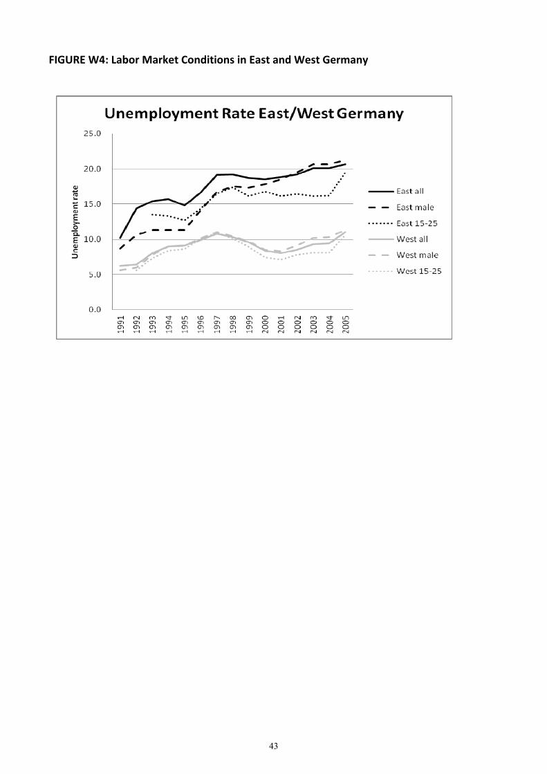
FIGURE W4: Labor Market Conditions in East and West Germany

43

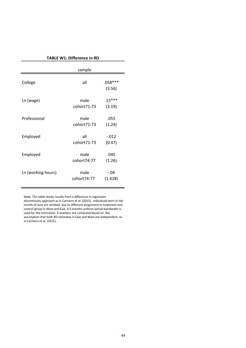
sample

College all .058***(3.56)

Ln (wage) male .15***cohort71‐73 (3.19)

Professional male .055cohort71‐73 (1.24)

Employed all ‐.012cohort71‐73 (0.47)

Employed male .045cohort74‐77  (1.26)

Ln (working hours) male ‐.04cohort74‐77  (1.418)

TABLE W1: Difference in RD

Note: This table shows results from a difference in regression discontinuity approach as in Carneiro et al. (2015).  Individuals born in the month of June are omitted, due to different assignment in treatment and control group in West and East. A 5 months uniform kernel bandwidth is used for the estimation. Z‐statistics are computed based on  the assumption that both RD estimates in East and West are independent, as in Carneiro et al. (2015). 

44

Dependent variable:                       (i) (ii) (iii) (iv) (v) (vi)

East*Treated (Def. 1) .139** ‐.024*** .006(.058) (.007) (.008)

East*Treat*cohort71‐73 0.096 ‐.025*** .009(.081) (.008) (.007)

East*Treat*cohort74‐77 .182** ‐.022* .002(.080) (.011) (.007)

Sample all all all all all allObservations         139605 139605 139605 139605 139605 139605

     

TABLE W2: Alternative Measures of Educational AttainmentYears of Schooling Vocational Unlearned 

NOTE: In col. (i) and (ii) the dependent variable is  the number of years of schooling  (built following the methodology used by the GSOEP) , in col. (iii)and (iv) it is a dummy variable equal to one if the respondent  obtained a vocational degree as highest educational attainment, in col (v) and (vi) it is a dummy variable equal to one if the respondent  does not have any formal vocational degree (i.e. no college degree, no vocational degree, and no Fachschul‐degree). Controls  include age dummies, state of residence dummies, birth year dummies, a male dummy and month of birth. Treatment is defined according to Definition 1, that is respondents born between June and December are considered treated. Robust standard errors are in parentheses, and are clustered at the treatment‐birth year‐east group level. The sample consists of all respondents  aged between 31 and 35 and born between 1971 and 1977. Residents in the state of Berlin are dropped from the sample. *significant at the 10% level, ** significant at the 5% level, *** significant at the 1% level.  

45

Dependent variable:   (i) (ii) (iii) (iv) (v) (vi) (vii) (viii) (ix) (x) (xi) (xii)all males females all males females all males females all males females

Treat  ‐.012**  ‐.019** ‐.006 0.01 ‐.002  .024* ‐.015* ‐.016 ‐.012 ‐.006 ‐.019  .011(.006) (.007) (.008) (.008) (.006) (.013) (.008) (.012) (.014) (.007) (.013) (.009)

East*Treat  ‐.004 ‐0.001 ‐.007 ‐.013 .003  ‐.033 .022***  .028**  .013 .013 .027**  ‐.004(.010) (.008) (.016) (.009) (.006) (.022) (.006) (.012) (.014) (.009) (.013) (.015)

Controls x x x x x x x x x x x xObservations         139605 69090 70515 113086 60838 52248 106496 57487 49009 111995 60140 51855

TABLE W3: Labor Market OutcomesEmployed Ln (work hours)  Ln (wage) Professional

NOTE:  In Columns (i)‐(iii) the dependent variable is a dummy variable equal to one if the respondent  was employed at the time of the survey. In Columns (iv)‐(vi) the dependent variable is the log of the number of weekly working hours. In Columns (vii)‐(ix) the dependent variable is the log of wages (see the text for a  detailed explanation of how wages are calculated). In Columns (x) to (xii) the dependent variable is a dummy variable equal to one if the respondent is either a manager or a professional according to the ISCO classification. Controls  include age dummies, state of residence dummies, birth year dummies, a male dummy, and month of birth. Treatment is defined according to Definition 1, that is respondents born between June and December are considered treated. Robust standard errors are in parentheses, and are clustered at the treatment‐birth year‐east group level.  The sample consists of all respondents  aged between 31 and 35 and born between 1971 and 1977. Residents in the state of Berlin are dropped from the sample. *significant at the 10% level, ** significant at the 5% level, *** significant at the 1% level.  

46

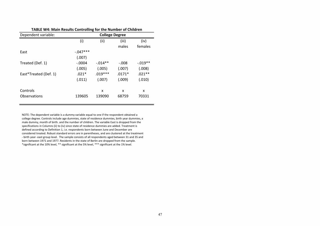
Dependent variable:  (i) (ii) (iii) (iv)

males femalesEast  ‐.047***

(.007)Treated (Def. 1) ‐.0004 ‐.014** ‐.008 ‐.019**

(.005) (.005) (.007) (.008)East*Treated (Def. 1) .021* .019*** .0171* .021**

(.011) (.007) (.009) (.010)

Controls x x xObservations         139605 139090 68759 70331

TABLE W4: Main Results Controlling for the Number of ChildrenCollege Degree

NOTE: The dependent variable is a dummy variable equal to one if the respondent obtained a college degree. Controls include age dummies, state of residence dummies, birth year dummies, a male dummy, month of birth. and the number of children. The variable East is dropped from the specifications in Columns (ii) to (iv) since state of residence dummies are added. Treatment is defined according to Definition 1, i.e. respondents born between June and December are considered treated. Robust standard errors are in parentheses, and are clustered at the treatment ‐ birth year‐ east group level.  The sample consists of all respondents aged between 31 and 35 and born between 1971 and 1977. Residents in the state of Berlin are dropped from the sample. *significant at the 10% level, ** significant at the 5% level, *** significant at the 1% level.

47

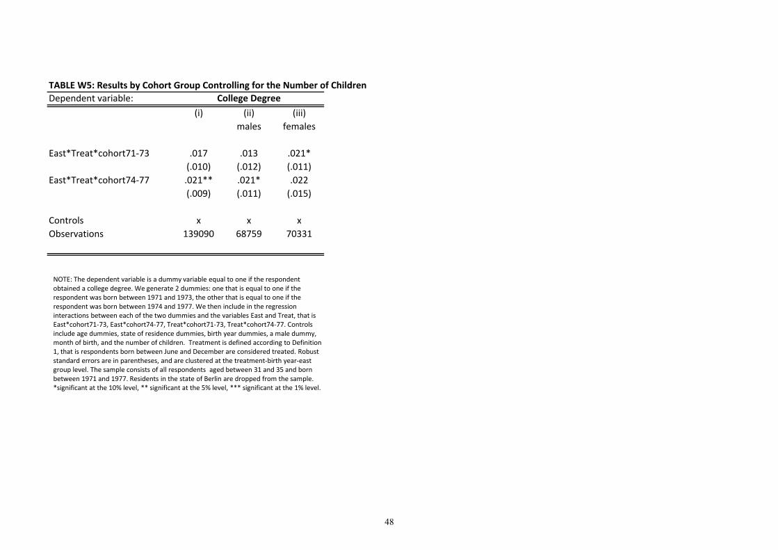
TABLE W5: Results by Cohort Group Controlling for the Number of ChildrenDependent variable:   

(i) (ii) (iii)males females

East*Treat*cohort71‐73 .017 .013 .021*(.010) (.012) (.011)

East*Treat*cohort74‐77 .021** .021* .022(.009) (.011) (.015)

Controls x x xObservations         139090 68759 70331

College Degree

NOTE: The dependent variable is a dummy variable equal to one if the respondent obtained a college degree. We generate 2 dummies: one that is equal to one if the respondent was born between 1971 and 1973, the other that is equal to one if the respondent was born between 1974 and 1977. We then include in the regression interactions between each of the two dummies and the variables East and Treat, that is East*cohort71‐73, East*cohort74‐77, Treat*cohort71‐73, Treat*cohort74‐77. Controls  include age dummies, state of residence dummies, birth year dummies, a male dummy, month of birth, and the number of children.  Treatment is defined according to Definition 1, that is respondents born between June and December are considered treated. Robust standard errors are in parentheses, and are clustered at the treatment‐birth year‐east group level. The sample consists of all respondents  aged between 31 and 35 and born between 1971 and 1977. Residents in the state of Berlin are dropped from the sample. *significant at the 10% level, ** significant at the 5% level, *** significant at the 1% level.

48

Dependent variable:   (i) (ii) (iii) (iv) (v) (vi) (vii) (viii) (ix) (x) (xi) (xii)all males females all males females all males females all males females

East*Treat*cohort71‐73 ‐.024**  ‐.025** ‐.023  ‐.021* ‐.009  ‐.037  .028*** .041*** .010  .024** .05***  ‐.007(.009) (.011) (0.015) (.010) (.008) (.025) (.007) (.013) (.016) (.012) (.01) (.014)

East*Treat*cohort74‐77 .016 .02*** .009 ‐.004 .015***  ‐.031 .013  .006 .017 ‐.0003 .003  ‐.003(.009) (.004) (0.016) (.009) (.005) (.026) (.011) (.010) (.014) (.006) (.015) (.022)

Controls x x x x x x x x x x x xObservations         139090 68759 70331 112806 60674 52132 106247 57335 48912 111742 59993 51749

Employed Ln (work hours)  Ln (wage) ProfessionalTABLE W6: Labor Market Outcomes Controlling for the Number of Children 

NOTE:  In Columns (i)‐(iii) the dependent variable is a dummy variable equal to one if the respondent  was employed at the time of the survey. In Columns (iv)‐(vi) the dependent variable is the log of the number of weekly working hours. In Columns (vii)‐(ix) the dependent variable is the log of wages (see the text for a  detailed explanation of how wages are calculated). In Columns (x) to (xii) the dependent variable is a dummy variable equal to one if the respondent is either a manager or a professional according to the ISCO classification. We generate 2 dummies: one that is equal to one if the respondent was born between 1971 and 1973, the other that is equal to one if the respondent was born between 1974 and 1977. We then include in the regression interactions between each of the two dummies and the variables East and Treat, that is East*cohort71‐73, East*cohort74‐77, Treat*cohort71‐73, Treat*cohort74‐77. Controls  include age dummies, state of residence dummies, birth year dummies, a male dummy, month of birth, and the number of children. Treatment is defined according to Definition 1, that is respondents born between June and December are considered treated. Robust standard errors are in parentheses, and are clustered at the treatment‐birth year‐east group level.  The sample consists of all respondents  aged between 31 and 35 and born between 1971 and 1977. Residents in the state of Berlin are dropped from the sample. *significant at the 10% level, ** significant at the 5% level, *** significant at the 1% level.  

49

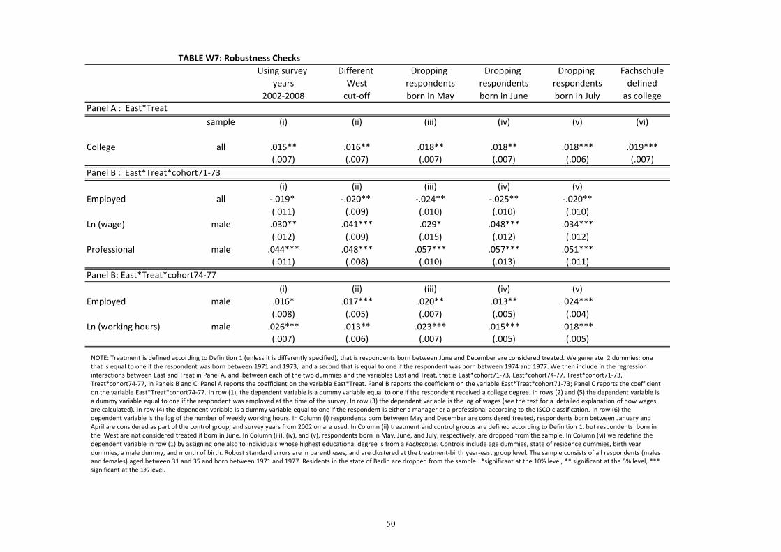
Using survey  Different  Dropping  Dropping  Dropping  Fachschuleyears West respondents respondents respondents defined

2002‐2008 cut‐off born in May born in June born in July as collegePanel A :  East*Treat                     sample (i) (ii) (iii) (iv) (v) (vi)

College all .015** .016** .018** .018** .018*** .019***(.007) (.007) (.007) (.007) (.006) (.007)

Panel B :  East*Treat*cohort71‐73                     (i) (ii) (iii) (iv) (v)Employed all ‐.019*  ‐.020**  ‐.024** ‐.025** ‐.020**

(.011) (.009) (.010) (.010) (.010)Ln (wage) male .030** .041*** .029* .048*** .034***

(.012) (.009) (.015) (.012) (.012)Professional male .044*** .048*** .057*** .057*** .051***

(.011) (.008) (.010) (.013) (.011)Panel B: East*Treat*cohort74‐77                      (i) (ii) (iii) (iv) (v)Employed male .016* .017*** .020** .013** .024***

(.008) (.005) (.007) (.005) (.004)Ln (working hours) male .026*** .013** .023*** .015*** .018***

(.007) (.006) (.007) (.005) (.005)

TABLE W7: Robustness Checks

NOTE: Treatment is defined according to Definition 1 (unless it is differently specified), that is respondents born between June and December are considered treated. We generate  2 dummies: one that is equal to one if the respondent was born between 1971 and 1973,  and a second that is equal to one if the respondent was born between 1974 and 1977. We then include in the regression interactions between East and Treat in Panel A, and  between each of the two dummies and the variables East and Treat, that is East*cohort71‐73, East*cohort74‐77, Treat*cohort71‐73, Treat*cohort74‐77, in Panels B and C. Panel A reports the coefficient on the variable East*Treat. Panel B reports the coefficient on the variable East*Treat*cohort71‐73; Panel C reports the coefficient on the variable East*Treat*cohort74‐77.  In row (1), the dependent variable is a dummy variable equal to one if the respondent received a college degree. In rows (2) and (5) the dependent variable is a dummy variable equal to one if the respondent was employed at the time of the survey. In row (3) the dependent variable is the log of wages (see the text for a  detailed explanation of how wages are calculated). In row (4) the dependent variable is a dummy variable equal to one if the respondent is either a manager or a professional according to the ISCO classification. In row (6) the dependent variable is the log of the number of weekly working hours. In Column (i) respondents born between May and December are considered treated, respondents born between January and April are considered as part of the control group, and survey years from 2002 on are used. In Column (ii) treatment and control groups are defined according to Definition 1, but respondents  born in the  West are not considered treated if born in June. In Column (iii), (iv), and (v), respondents born in May, June, and July, respectively, are dropped from the sample. In Column (vi) we redefine the dependent variable in row (1) by assigning one also to individuals whose highest educational degree is from a Fachschule. Controls include age dummies, state of residence dummies, birth year dummies, a male dummy, and month of birth. Robust standard errors are in parentheses, and are clustered at the treatment‐birth year‐east group level. The sample consists of all respondents (males and females) aged between 31 and 35 and born between 1971 and 1977. Residents in the state of Berlin are dropped from the sample.  *significant at the 10% level, ** significant at the 5% level, *** significant at the 1% level.  

50

Panel A :  East*Treatsample

College all  ‐.006(.011)

Panel B :  East*Treat*cohort71‐73

Employed all  .011(.012)

Ln (wage) male .023(.017)

Professional male .001(.020)

Panel B: East*Treat*cohort74‐77 

Employed male  ‐.031(.021)

Ln (working hours) male ‐.003(.008)

TABLE W8: Placebo Exercise

NOTE: We generate  2 dummies: one that is equal to one if the respondent was born between 1971 and 1973,  and a second that is equal to one if the respondent was born between 1974 and 1977. We then include in the regression interactions between East and Treat in Panel A, and  between each of the two dummies and the variables East and Treat, that is East*cohort71‐73, East*cohort74‐77, Treat*cohort71‐73, Treat*cohort74‐77, in Panels B and C. Panel A reports the coefficient on the variable East*Treat. Panel B reports the coefficient on the variable East*Treat*cohort71‐73; Panel C reports the coefficient on the variable East*Treat*cohort74‐77. In row (1), the dependent variable is a dummy variable equal to one if the respondent received a college degree. In rows (2) and (5) the dependent variable is a dummy variable equal to one if the respondent was employed at the time of the survey. In row (3) the dependent variable is the log of wages (see the text for a  detailed explanation of how wages are calculated). In row (4) the dependent variable is a dummy variable equal to one if the respondent is either a manager or a professional according to the ISCO classification. In row (6) the dependent variable is the log of the number of weekly working hours. Respondents born between October and December are considered treated, respondents born between July and September are considered the control group. Controls include age dummies, state of residence dummies, birth year dummies, a male dummy, and month of birth. Robust standard errors are in parentheses, and are clustered at the treatment‐birth year‐east group level. The sample consists of all respondents (males and females) aged between 31 and 35 and born between 1971 and 1977. Residents in the state of Berlin are dropped from the sample. *significant at the 10% level, ** significant at the 5% level, *** significant at the 1% level.  

51

Panel A :  East*Treatsample (i) (ii) (iii) (iv) (v) (vi) (vii) (viii) (ix) (x) (xi)

UR (plus sq) male UR (plus sq) youth UR  youth UR  state UR state UR  state male UR state male UR  state youth UR state youth UR market entr. trends*state(plus sq) (plus sq) (plus sq) (plus sq)

College all .019** .019*** .021** .023** .020*** .018** .020*** .018*** .020*** .020*** .016**(.007) (.006) (.009) (.010) (.007) (.006) (.006) (.006) (.008) (.008) (.007)

Panel B :  East*Treat*cohort71‐73sample (i) (ii) (iii) (iv) (v) (vi) (vii) (viii) (ix) (x) (xi)

Employed all ‐.020* ‐.025** ‐.020** ‐.020* ‐.023** ‐.024** ‐.022**(.010) (.010) (.009) (.010) (.009) (.009) (.011)

Ln (wage) male .034*** .041*** .035*** .034*** .044*** .044*** .029***(.009) (.012) (.008) (.009) (.011) (.012) (.010)

Professional male .041*** .050*** .046*** .042*** .055*** .053*** .039***(.009) (.008) (.008) (.009) (.010) (.010) (.010)

Panel C: East*Treat*cohort74‐77 sample (i) (ii) (iii) (iv) (v) (vi) (vii) (viii) (ix) (x) (xi)

Employed male .016*** .018*** .021*** .019*** .022*** .020*** .025*** .023*** .021*** .022*** .015**(.005) (.005) (.005) (.005) (.004) (.004) (.006) (.005) (.004) (.005) (.006)

Ln (working hours) male .012** .011** .015*** .013** .015*** .014*** .014*** .013*** .015*** .013** .010**(.004) (.005) (.005) (.005) (.004) (.004) (.005) (.004) (.005) (.005) (.005)

TABLE W9: Robustness Checks‐Unemployment in Year of Labor Market Entrance 

NOTE: Treatment is defined according to Definition 1, that is respondents born between June and December are considered treated. We generate  2 dummies: one that is equal to one if the respondent was born between 1971 and 1973, the other that is equal to one if the respondent was born between 1974 and 1977. We then include in the regression interactions between each of the two dummies and the variables East and Treat, that is East*cohort71‐73, East*cohort74‐77, Treat*cohort71‐73, Treat*cohort74‐77. Panel A reports the coefficient on the variable East*Treat; Panel B reports the coefficient on the variable East*Treat*cohort71‐73; Panel C reports the coefficient on the variable East*Treat*cohort74‐77. In row (1) the dependent variable is a dummy equal to one if the respondent obtained a college degree. In rows (2) and (5) the dependent variable is a dummy variable equal to one if the respondent was employed at the time of the survey. In row (3) the dependent variable is the log of wages (see the text for a  detailed explanation of how wages are calculated). In row (4) the dependent variable is a dummy variable equal to one if the respondent is either a manager or a professional according to the ISCO classification. In row (6) the dependent variable is the log of the number of weekly working hours. Controls  include age dummies, state of residence dummies, birth year dummies, and gender.  Column (i) adds the East/West unemployment rate in the year of labor market entrance as a control in levels and squared, column (ii) the respective male unemployment rate in levels and squared, column (iii) the youth unemployment rate for individuals aged 15‐24, column (iv) the respective youth unemployment rate in levels and squared, column (v) adds the state unemployment rate in the year of labor market entrance as a control in levels, column (vi) adds the state unemployment rate in the year of labor market entrance as a control in levels and squared, column (vii) adds the state male unemployment rate in the year of labor market entrance as a control in levels, column (viii) adds the state male unemployment rate in the year of labor market entrance as a control in levels and squared, column (ix) adds the state youth unemployment rate in the year of labor market entrance as a control in levels, column (x) adds the state youth unemployment rate in the year of labor market entrance as a control in levels and squared, column (xi) state‐specific linear trends in the year of market entrance. Robust standard errors are in parentheses, and are clustered at the treatment‐birth year‐east group level. The sample consists of all respondents (males and females) aged between 31 and 35 and born between 1971 and 1977 (in col.  (iii), (viii) and (ix) we restrict the sample to cohorts 1974‐1977 due to data limitation). Residents in the state of Berlin are dropped from the sample.  *significant at the 10% level, ** significant at the 5% level, *** significant at the 1% level.  

52

Dependent variable:  Change of residence(i) (ii)

Treated (Def. 2) 0.0003 0.0002(.0013) (.0011)

Controls xObservations         73713 73713

TABLE W10: Migration Decisions

NOTE: The dependent variable is a dummy variable equal to one if the respondent moved from East to West Germany  in the year before the survey. Controls include age dummies, birth year dummies and a male dummy. Treatment is defined according to Definition 2, that is respondents born between May and December are considered treated. Therefore all available surveys (1991‐2008) are employed. Robust standard errors are in parentheses, and are clustered at the treatment‐birth year level. The sample consists of all respondents aged between 31 and 35 and born between 1971 and 1977 and resident in East Germany in the year before the survey. Residents in the state of Berlin are dropped from the sample. *significant at the 10% level, ** significant at the 5% level, *** significant at the 1% level.

53

YearCoefficient Standard error

1991 .00028 .004131992 ‐.00736* .003781993 .00738** .003551994 ‐.00155 .003201995 .00523 .003551996 ‐.00281 .003511997 .00690* .003791998 ‐.00259 .003511999 .00026 .003952000 ‐.00390 .004392001 .00462 .005532002 ‐.00526 .004492003 .00052 .004442005 .00021 .002652008 ‐.00047 .00186

TABLE W11: Migration Decisions Year by YearTreated (Def. 2)

NOTE: Each row  corresponds to a regression using  as a  sample only the survey year indicated and shows the coefficient  and the standard error of the variable "Treated". The dependent variable is a dummy variable equal to one if the respondent moved from East to West Germany  in the year before the survey. Controls include age dummies, birth year dummies anda male dummy. Treatment is defined according to Definition 2, that is respondents born between May and December are considered treated. The sample consists of all respondents aged between 31 and 35 and born between 1971 and 1977 and resident in East Germany in the year before the survey. Residents in the state of Berlin are dropped from the sample. *significant at the 10% level, ** significant at the 5% level, *** significant at the 1% level.  

54