long memory a ne term structure models - usi - eco · long memory a ne term structure models adam...

Long Memory AffineTerm Structure Models∗

Adam Golinski Paolo Zaffaroni

This draft: 21th November 2013

Abstract

We develop a Gaussian discrete time essentially affine term structure model whichallows for long memory. This feature reconciles the strong persistence observed innominal yields and inflation with the theoretical implications of affine models, especiallyfor long maturities. We characterise the dynamic and cross-sectional implications, inparticular in terms of volatility, of long memory for our model both under the physicaland risk-neutral measure. We explain how long memory can naturally arise within theterm structure of interest rates, providing a theoretical underpinning for our model.Despite the infinite-dimensional structure that long memory implies, we show how tocast the model in state space and estimate it by maximum likelihood. As an example,we estimate a two-factor version of the model whereby the unobserved factors have aclear economic interpretation as the real short rate and expected inflation.

∗Golinski: University of York, Department of Economics and Related Studies, Heslington, York, YO105DD, UK. E-mail: [email protected]: Imperial College Business School, Imperial College London, South Kensington Campus, London,SW7 2AZ, UK. E-mail: [email protected].

1

1. Introduction

Modelling the term structure of interest rates is a relevant from many different perspec-tives, both academic and practical. For instance, central bankers would be interested inextracting inflation expectations and future movements of short rates embedded in nomi-nal yields. From a macroeconomics angle, deriving the term structure of real interest ratesallows to measure the cost of investment and its implication for economic growth. From afinance perspective, it is crucial to price accurately nominal and inflation-indexed bonds andassociated term premia.

The main challenge is that nominal observed yields are extremely persistent, in fact hardlydistinguishable from a nonstationary series. A routine test would hardly reject the hypothesisof a unit root. Although explicitly assumed in early work of term structure modelling (seeDothan (1978)), accepting the possibility of a unit root in the physical measure appearstroublesome in terms of its economics implications and econometric estimation. In fact,the unit root paradigm rules out any degree of mean-reversion, namely the possibility thatshocks are eventually absorbed as time goes by. Lack of mean-reversion bears un-plausiblecross-sectional predictions, in particular in terms of the volatility term structure of yields,forward rates and holding period returns. In terms of estimation, the unit root affects thefinite sample as well as the asymptotic properties of conventional estimators of term structuremodels, making inference more difficult. Recognising that the notion of long memory permitsto obtain a substantial degree of persistence, in fact even non stationarity, together withdynamic mean-reversion, this paper develops a class of discrete time no-arbitrage affine termstructure models with long memory state variables. The idea of long memory has beenpostulated as a suitable description of nominal yields by Backus and Zin (1993), whichcan be seen as a very special case of our general theory1. Here also provide a theoreticalfoundation for the presence of long memory in term structure models.

Our long memory model belongs to the class of essentially affine (in the sense of Con-stantinides (1992), Duffe (2002) and Dai and Singleton (2002)) conditionally Gaussian termstructure model with multiple factors. We establish the closed-form solution of the modeland, relying on its state space representation, show how to carry out estimation by maxi-mum likelihood and Kalman filtering of the latent state variables. These achievements arenon trivial because a critical feature of long memory models is to be non-Markov implying,in our affine term structure context, infinite-dimensional state variables.

Our approach shares the many virtues of the powerful class of affine models, formallydefined by Duffie and Kan (1996) and pioneered by Vasicek (1977) and Cox, Ingersoll andRoss (1985) highly influential models. First, closed-form solution for bond prices and yieldscan be easily obtained as affine functions of a set of state variables. Second, nominal yieldscan be decomposed into inflation expectations, real yields and inflation risk premia withminimal, no-arbitrage, assumptions. Third, conditional moments, in particular term premia,can be easily computed. Fourth, the model can be naturally casted in state-space implyingthat parameters estimation and inference can be obtained by maximum likelihood estimation.Filtered values of the latent state variables, which typically include expected inflation and

1Related work is also Comte and Renault (1996) who analyse a continuous time long memory model andthe equilibrium approach of Duan and Jacobs (1996) where long memory enters through the volatility ofstate variables.

2

the short-term real interest rate, follow by the Kalman recursion.To better understand the analogies, and differences, of our model with the conventional

affine models, it is useful to consider the unified framework represented by the class DAQM(N)

of discrete-time affine models spelled out by Le, Singleton and Dai (2010)2, where M of theN factors (here 0 ≤ M ≤ N) drive stochastic volatility. Gaussian affine models, wherebythe unconditional distribution of the state vectors is normal, feature M = 0 (no stochasticvolatility) and makes the DAQ

0 (N) class. A crucial feature of the DAQ0 (N) class is that,

under the risk-neutral (Q) measure, the N state variables form a Markov system, possiblyof higher yet finite order, such as a vector autoregression. It is well known that the Markovproperty, with stationarity, implies a weak form of temporal dependence for model-impliedyields, as expressed by the fast decay toward zero of the theoretical autocorrelation function.Moreover, this form of strong mean-reversion implies that the theoretical volatility, bothconditional and unconditional, of long yields and forward rates diminishes fast toward zeroas maturity increases. At the same time, the model-implied volatility of holding periodreturns stays bounded for large maturities. These features are completely at odds withthe empirical evidence. However, if one relaxes the assumption of stationarity under the Qmeasure, within the DAQ

0 (N) class, a unit or even an explosive root emerges the consequencesof which are also at odds with the empirical evidence. As discussed above, this rules outdynamic mean-reversion and for instance, in the unit root case the theoretical (conditional)volatility of yields and forward rates is flat across maturity whereas it increases quasi linearlyfor returns.

In contrast, due to the long memory specification of our model, we are able to matchthe strong degree of persistence together with the slow degree of dynamic mean-reversionobserved in nominal yields. When looking at the characteristics across maturity, our model-driven term structure of volatility for yields and forward rates can be slowly decaying forintermediate maturities yet flattening out or even slowly increasing for long maturities. Atthe same time, the model-driven volatility term structure will slowly diverge for returns.These are the features observed in the data. As we shall see, long memory can be obtainedby allowing the number of state variables, N , to become infinite, spanning the DAQ

0 (∞)class of term structure models, with respect to the Le, Singleton and Dai (2007) notation.Besides infinite-dimensionality of the state variables, a suitable long lags characterization ofthe state variables impulse response is required in order to induce long memory.

Obviously these various issues raised by the persistence in nominal bond data have at-tracted a great deal of interest and different approaches have been developed. These arereviewed in Appendix C, where we discuss their analogies with our long memory framework.

Although our theory is completely general, we then present a model that includes re-alised inflation within the set of observables, and thus expected inflation as one of the statevariables. This makes our model akin to terms structure models that merge yields andmacroeconomic data, such as the DAQ

0 (N)-type models of Ang and Piazzesi (2003), Rude-bush and Wu (2008) and Hordhalh, Tristani and Vestin (2008) among others. Includinginflation is instrumental for recovering the canonical decomposition of nominal yields into

2This class nests all the exact discrete-time representation of the general class of continuous-time modelsof Dai and Singleton (2000). Under the physical measure this class of models might feature nonlinearity butare characterised by a closed-form expression of the exact likelihood.

3

the term structure of real yields, inflation expectation and inflation risk premia3. It is alsoasked for by the data. In fact long memory appears to be a robust description of realisedinflation dynamics. Altissimo et al (2009) analyse how the consumer price index (hereafterCPI) construction protocol gives rise naturally to long memory in CPI inflation and provideempirical evidence for the inflation rate of the euro area. As a consequence, inflation appearsto be one of the main channels that naturally leads to long memory in observed nominalyields, as argued below.

Since Rogers (1997), it is well known that assuming long memory for a tradable assetmight lead to existence of arbitrage opportunities. This would undermine the possibility toidentify the pricing kernel and thus, in our case, to determine model-implied (bond) prices.However, it is now understood that the conditions required to violate no-arbitrage are muchmore stringent in a discrete time setting (see Cheridito (2003)) such as ours. Moreover,arbitrage opportunities are ruled out whenever transaction costs, no matter how minimal,are allowed for, ensuring existence and uniqueness of the pricing kernel (see Guasoni, Rasonyiand Schacher- mayer (2010)). Therefore, as discussed below, no pricing consequence for ourmodel appears to arise despite its long memory feature.

The paper proceeds as follows. Section 2 describes the data for nominal yields and infla-tion used for estimation of the model. We highlight some features of the yields data, namelytheir dynamic persistence and the shape of their volatility term structure, especially for longmaturities. Section 3 explores the extent to which these features can be accounted for byVasicek-type model, spelling out the theoretical implication for long term yields, forwardrates and returns. This paves the ground for the long memory model. Section 4 presents thelong memory model: a discrete time essentially affine non-Markov Gaussian term structuremodel. With no loss of generality, we focus on the case of two latent factors and establishclosed-form solution of the model for a general parameterization of the state variables dy-namics, in terms of the nominal and real term structures. Section 4.4. provides analyticalcharacterization of the time series and cross-sectional properties, in terms of volatility termstructure of yields, forward rates and holding period returns, under both the physical andQ measure, shedding light on the critical role of long memory. Section 5 discusses theoret-ical underpinnings of long memory in real and nominal yields, leaving some formal detailsto Appendix A. Estimation results are described in Section 6. A technical description ofthe Kalman filter and an approximate maximum likelihood estimator for long memory pro-cesses is relegated to Appendix D. Having estimated a simple two-factor version of the longmemory model, we verify in Section 6.1 that the above described features of the empiricaldistribution of zero coupon bonds are extremely well matched by the model. The estimatedtwo-factor model is rich enough to decompose nominal yields into the real interest rate, in-flation expectation and the inflation risk premia term structures, as exemplified in Section6.3. Some indications on the statistical performance of the estimated long memory model areexamined in Section 6.4. Section 6.4.2 presents some out-of-sample forecasting performanceresults, comparing our affine long memory model with well-established models such as Ang

3Alternative methods for recovering the real term structure and inflation expectation uses inflation-indexed bonds (see Barr and Campbell (1997) and Evans (1998) among others), Treasury inflation-protectedsecurities (see D’Amico et al (2008) and Christensen et al (2010) and among others), survey forecasts ofinflation (see Pennacchi (1991) and Chernov and Mueller (2012) among others) and inflation-based derivatives(see Haubrich et al (2012) and Kitsul and Wright (2012)).

4

and Piazzesi (2003) macro model, Ang, Bekaert and Wei (2008) regime switching model andDiebold and Li (2006) cross-sectional model. Final remarks makes Section 7. Appendix Aexplains how long memory can be induced within the class of affine term structure models.Appendix B discusses the pricing implications of long memory for our model. A review ofthe different approaches to tackle the high persistence of observed nominal yields, and theiranalogies with our long memory approach, are discussed in Appendix C. Particular empha-sis is given to regime switching term structure models. Appendix E contains two technicallemmas and the proofs of the main theorems.

2. Some stylised facts of nominal bonds and inflation

We now highlights the strong, well established, degree of dynamic persistence that char-acterises certain specific aspects of our interest of the empirical distribution of nominal bondsand consumer price index (CPI) inflation. Regarding nominal bonds, we consider the termstructure of nominal yields, forward rates and holding period returns. Noticeably, we wishto emphasise how the extremely strong degree of time series persistence, measured in a wayspecified below, appears to influence certain cross-sectional aspects of the yields distribution,namely the term structure of volatility, of nominal yields, forward rates and returns. In par-ticular, this strong persistence appears to be the main channel through which the negligiblevolatility of bond returns at very short maturities becomes magnified by several orders ofmagnitude as we move along the term structure. Similarly, the riskiness of long term yieldsand forward rates appear only slowly declining along the term structure, far from vanishingfor very long maturities. These stylised facts can be qualitatively rationalised by means ofa simple Markov term structure model, as exemplified in Section 3. However, anticipatingmatters, when looking more carefully, both the time series and the cross-sectional evidenceappear at odd with the quantitative predictions of such term structure model built aroundboth stationary and non-stationary Markov state variables.

2.1. Nominal bonds

This section uses a data set comprised of monthly observations of nominal yields r$n,t on

zero coupon bonds with maturities n equal to 1 and 3 month, 1, 3, 5, 10, 15, 20− and 30 year.The source for the 1 and 3 month yields is the Fama’s Treasury bills term structure files,while for maturities up to 5 year are the Fama-Bliss discount bond files. The 10 to 30 yearare obtained using the approach of Gurkaynak et al (2007). The data are available fromNovember 1985 to December 2011. Yields

r$t,ni

= − 1

nilogPnit,

are continuously compounded, annualised and percent, where Pnit denotes nominal zerocoupon bond prices with maturity ni. We also consider (nominal) forward rates

f $t,ni,ni+1

= (ni+1r$ni+1,t

− nir$ni,t

)/(ni+1 − ni) with maturities ni < ni+1,

5

and holding period returns

y$t,ni−1,ni

= (nir$ni,t−(ni−ni−1) − ni−1r

$ni−1,t

)/(ni − ni−1) with maturities ni−1 < ni.

Summary statistics are presented in Table 1.

[Insert Table 1 near here]

Average yields are increasing with maturity whereas their volatility, expressed in termsof standard deviation, shows a hump at about one year maturity and then flattens out.A similar pattern is obtained in terms of forward rates, the main difference being that forforward their volatility term structure raises sharply again for long maturitities after decliningfrom the one-year hump. Holding period returns exhibit a monotonically increasing volatilitycurve.

It has been known for a long time that nominal yields display a substantial degree ofpersistence4. This is evident when performing unit root tests, as illustrated Table 2 wherewe present the results for the standard Augmented Dickey-Fuller (ADF) unit root test.


The null hypothesis of unit root is not rejected for nominal yields across all maturities.However, the unit root paradigm rules out mean-reversion, which appears implausible froman empirical and theoretical viewpoint. Moreover, as exemplified below, unit root dynamicsraises implausible cross-sectional predictions within affine term structure models.

We propose to assess the persistence of nominal bonds characteristics using a somewhatmore sophisticated approach that does not suffer the limits of the unit root framework. Inparticular, we need to use a measure that allows to disentangle the notion of nonstationarityfrom the one of mean-reversion.

Figure 1(a) plots the periodogram ordinates near the zero frequency for yields, forwardand returns, averaged across maturity5 where for a sample of generic observables (w1, ...wT )the periodogram is

Iw(λ) =1

2πT

∣∣∣∣∣T∑t=1

wteıλt

∣∣∣∣∣2

, −π < λ ≤ π.

Data have been standardised so that they sample variance is unity.

[Insert Figure 1 near here]

The strength of the periodogram are essentially that is a nonparametric measure andthat it is a function of the entire strings of sample autocorrelation of the data. In general, itgives neat insights on both the low, medium and high frequency dynamics of the data, whichin turn are linked to the long run persistence, mean-reversion, and cycles of the data. Forinstance, the periodogram near zero frequency is proportional to the sum of the entire set ofsample autocorrelations corresponding to a given sample and, as such, is a clearcut measure

4See for example Ball and Torous (1996) and Kim and Orphanides (2012) among many others.5The same pattern is observed for the single maturities with little variation.

6

of persistence6. Instead, the local behaviour of the periodogram, as one moves away fromthe zero frequency, provides indications on the degree of mean-reversion.

Given the substantial mass of the periodogram of the data near zero frequency, it ismore insightful to examine the log periodogram where large values of the periodogram aremitigated. Figure 1(b) clearly shows that yields, forward and returns all display a negativelysloped log-periodogram near the origin, for at least the first twenty or thirty frequencies.

To provide a benchmark, any stationary autoregressive moving average (ARMA) pro-cess implies a zero-sloped logarithm of the spectral density near the zero frequency. Weplot the spectral density for AR(1) model with unit variance with autoregressive parameterequal to 0.80, 0.98, 0.99999, represented by the the blue, red and green line, respectively, inFigure 2(a). Figure 2(b) reports the same quantities in the logarithmic scale.


The comparison is striking: even a value as large as 0.98 does not induce a sufficientdegree of persistence, as expressed by a peak near zero of the periodgram, able to matchthe peak found in the data. The mean-reversion implied by stationary ARMA is also toostrong. The case of autoregressive parameter equal to 0.99999 appears more akin to thedata at zero frequency. However, for this case it would be hard to deny the existence of aunit root. Moreover, although dense near zero, the behaviour of the log-spectrum with anautoregressive parameter of 0.99999 does not match too well the other higher frequencies, inparticular the slow, hyperbolic, decay of the log periodogram of the data as the frequencyincreases. We interpret this a the limit of the unit root paradigm, able to induce persistencebut at the cost of giving up stationarity and, in particular, mean-reversion. As it will shownbelow, this provides implausible predictions for the volatility cross-section of nominal bondcharacteristics across maturities.

We summarize this finding as follows.Stylized Fact 1. Nominal yields, forward and holding period returns are highly persistentacross time yet mean reverting. In particular they all display a negatively sloped log peri-odogram near the origin, slowly decaying as the frequency increases.

Figure 3(a) displays the term structure of the sample standard deviation of yields and for-ward rates. As observed in Table 1, for yields, the curve is decaying yet with a hump at abouttwo year maturity, flattening for longer maturities at about 3% and in any case well abovezero. Forward rates have a similar pattern, although they show an even more substantialincrease toward the end of the term structure, clearly non vanishing with maturity.


Figure 3(b) reproduces the term structure of the sample standard deviation of holdingperiod returns. It clearly emerges how, differently from yields and forward rates, the volatilityof returns raises steeply with maturity. These observations lead to:

6In fact the periodogram can be rewritten as Iw(λ) = (1/2π)∑T−1k=−T+1 ˆcovw(k)eıkλ for λ 6= 0 where

ˆcovw(k) = T−1∑T−|k|t=1 (wt − w)(wt+|k| − w), namely the sample autocovariance at lag k (see Brockwell and

Davis (1991), Proposition 10.1.2).

7

Stylized Fact 2. The term structure of the sample standard deviation of nominal yieldsand forward rates slowly declines up to mid maturities and then flattens out or even slowlyincreases for long maturities. The term structure of the sample standard deviation of nominalholding period returns rises with maturity without flattening out.

These facts are well documented in the term structure literature. The approach proposedin this paper tries to explain these features of persistence and yet slow mean-reversion.Note that although Stylized Fact 1 is a time series characteristic, Stylized Fact 2 featurescross-sectional aspects of the bond data. However, these are intimately related and can berationalised within an affine framework.

2.2. Inflation

Data is taken from Bureau of Labor Statistics of U.S. Department of Labor, wheremonthly observations are available from from June 1947 to December 2011. We calculate(non seasonally adjusted) inflation based on the all urban consumer price index as:

πt = log(CPIt)− log(CPIt−1). (1)

In Table 1 we report the basic summary statistics where inflation is annualised and percent.The average inflation is 3.74% with a standard deviation of 3.57%. The last column of Table 2reports the Augmented Dickey-Fuller test for inflation. The unit root hypothesis now cannotbe rejected at 5% significance level. However, as for yields, we look at the more revealingplot of the log periodogram, reported in Figure 4. The periodogram of (normalized) inflationis plotted (blue line) together with the spectral density of autoregressive processes of orderone with parameters 0.80, 0.98 and 0.99999 (green, red and light blue line respectively), all ofwhich appear inadequate. The strong degree of persistence is evident yet with some featureof mean-reversion, as expressed by the slow decay as the frequency increases.


Persistence of CPI inflation, in particular in the form of long memory, has been doc-umented (for the euro area) in detail by Altissimo et al (2009) who argue that this is anunavoidable consequence of the way in which price indexes are constructed. This is revis-ited in Section 5 below. Persistence of observed inflation clearly reflects the persistence ofexpected inflation, the key variable in term structure modelling. This fact also suggests thatthe magnitude of the volatility of unexpected inflation (the difference between observed andexpected inflation), which by construction is serially uncorrelated across time, cannot be toolarge for otherwise it would mask the persistence found in the data.

3. Implications for Markov affine models

We now revisit the theoretical implications of the persistence of yields, found in the data,for Gaussian Markov affine models. Consider the discrete time version of the Vasicek (1977)model, a one-factor Gaussian model. The price of a real zero-coupon bond issued at time t

8

which expires n periods ahead, here denoted Qn,t, satisfies the no-arbitrage condition

Qn,t = Et (emt+1Qn−1,t+1) , (2)

where Et(·) is the expectation operator conditional on the information available up to time t,based on the physical measure. It is well-known that assuming no-arbitrage implies existenceof the real pricing kernel emt+1 which, for this model, has the simple form

−mt+1 = µr +1

2λ2σ2

x + xt + λεxt+1 (3)

where the (single) factor follows an AR(1) process

xt = ψxxt−1 + εxt, εxt ∼ NID(0, σ2x), (4)

and λ, µr, ψx, σ2x are constant parameters with | ψx |≤ 1.

By the standard recursive method one obtains that bond yields rt,n = −(1/n) logQn,t,forward rates fn,t and holding one-period returns satisfy, respectively,

rt,n = n−1(An +Bnxt), (5)

ft,n = An+1 − An + (Bn+1 −Bn)xt, (6)

yt,n = An − An−1 +Bnxt−1 −Bn−1xt, (7)

where, in turn, the n-varying coefficients satisfy the well-established Riccati difference equa-tions

An = An−1 + µr − λσxBn−1 −1

2B2n−1σ

2x, Bn = 1 + ψxBn−1, (8)

with initial conditions A0 = B0 = 0.Consider first the stationary case |ψx| < 1 giving Bn = (1−ψnx)/(1−ψx). Clearly yields,

forward rates and returns are elementary (linear) transformation of the AR(1) process xt,and their temporal dependence, under the physical measure, is determined by the magnitudeof ψx. Analytically, the spectral density for yields, forward rates and returns7 is, for −π ≤λ < π,

srn(λ) = B2n sx(λ),

sfn(λ) = (Bn −Bn−1)2 sx(λ),

srn(λ) = sx(λ) +B2n−1

σ2x

2π+ 2Bn−1

σ2x

2π<(

eıλ

1− ψxeıλ

),

where <(.) denotes the real part of a complex number, ı is the complex unit and sx(λ)indicates the spectral density of the AR(1) state variable (4), equal to σ2

x/(2π|1 − ψxeıλ|2).

7For returns the additional terms in the spectral density are due to the fact yt,n can be represented asAn−An−1 + xt−1−Bn−1εxt. However the behaviour of the first and third term in srn(λ) are identical nearthe zero frequency.

9

By easy derivations, the slope of the log spectra, for λ→ 0+, will then satisfy

dlog srn(λ)

d log λ∼ 2ψx

(1− ψx)2λ2,

dlog sfn(λ)

d log λ∼ 2ψx

(1− ψx)2λ2,

dlog sfn(λ)

d log λ∼(

2ψx(1− ψx)2

+2Bn−1(1−Bn−1ψx)

(1 +Bn−1(1− ψx))2

)λ2.

In all cases the slope becomes null at zero frequency and its magnitude, near zero frequency, islarger the closer ψx is to unity. This was already illustrated in Figure 2(b), which shows howthe log-spectral density becomes flat near the zero frequency approaching a positive finitevalue8 for ψx equal to 0.90 and 0.98, represented by the blue and green line respectively.

The term structures of conditional and unconditional volatility for yields, forward ratesand returns are

vart−1(rt,n) = (Bn

n)2σ2

x, var(rt,n) = (Bn

n)2 σ2

x

1− ψ2x

,

vart−1(ft,n) = ψ2nx σ

2x, var(ft,n) = ψ2n

x

σ2x

1− ψ2x

,

vart−1(yt,n) = B2nσ

2x, var(yt,n) = B2

nσ2x +

σ2x

1− ψ2x

,

where vart(·) is the variance operator conditional on the information available up to time t,based on the physical measure. Since Bn ∼ 1/(1− ψx) for large n when |ψx| < 1, it followsthat, as n→∞,

vart−1(rt,n) ∼(

σ2x

(1− ψx)2

)1

n2, vart−1(ft,n) ∼ ψ2n

x σ2x, vart−1(yt,n) ∼ σ2

x

(1− ψx)2, (9)

where ∼ indicates asymptotic equivalence9. An identical pattern is obtained for uncondi-tional variances. When |ψx| > 1 the conditional variances will all rapidly explode (approxi-mately for yields) as ψ2n

x for large n. These results are obtained under the implicit assump-tion, embedded in (3), of constant market price of risk. If one replaces λ by λt = λ0 + λ1xtinto (3), for some constant non-zero parameters λ0, λ1, the same formulae for the conditionalvariance term structures apply but with ψx replaced by ψx ≡ ψx− λ1σ

2x, the Q measure AR

coefficient.Consider now the unit root case ψx = 1 giving Bn = n. Now the model is nonstationary

under the physical measure so the variance is not finite and the spectral density is not defined,technically speaking. The quasi-unit root case ψx = 0.99999 reported in Figure 2(b), redline, shows how the log-spectrum will exhibit a sharp peak near zero frequency. The term

8Equivalently, the autocorrelation function is summable and, in particular, proportional to ψ|u|x at lag u.

9We say that an ∼ bn, where bn 6= 0, when an/bn → 1 as n→∞.

10

structure of conditional volatility for yields, forward rates and returns will now be

vart−1(rt,n) = σ2x, vart−1(ft,n) = σ2

x, vart−1(yt,n) = n2σ2x. (10)

The model is purposely extremely stylized, but it shares the main predictions in termsof persistence and of long maturity behaviour of the volatility term structures with moresophisticated discrete affine models with ARMA state variables.

In particular, the cases of both stationary and non-stationary ARMA state variables areat odd with the empirical evidence surveyed in Section 2. The stationary case generatesa stronger than needed degree of mean-reversion whereas the nonstationary, unit root orexplosive, case rules out mean-reversion altogether. Moreover, postulating a unit root makesinvalid the evaluation of impulse responses and variance decomposition. There appears theneed for a model able to generate an intermediate degree mean-reversion between these twocases, without imposing nonstationarity. This is accomplished by the long memory affineterm structure model, which we formalise in the next section.

4. Long memory affine term structure models: repre-

sentation

Long memory models, in particular autoregressive fractionally integrated moving average(ARFIMA) models, bridge the gap between stationary ARMA and ARIMA (when a unitroot is allowed for). In fact, not only long memory models can describe the dynamicsof stationary yet highly persistent time series but can also account for non-stationary yetmean reverting series, whereby the impulse response function will eventually die out withtime10. There is another, less known, feature of linear long memory models that makesthem particularly useful with respect to affine models, namely the fact that they admit astate-space representation although with infinite-dimensional state variables. This result hasbeen established by Chan and Palma (1998) and summarized in Appendix D. It turns outthat, despite the presence of an infinite number of transition equations, the likelihood can becomputed in a finite number of steps. Therefore parameter estimates can be obtained andthe Kalman filter delivers optimal out-of-sample forecasts and filtered values of the latentfactors.

These considerations suggest to consider Gaussian affine models with long memory statevariables. This model is described in the following subsections. We first show how to solvethe model imposing the no-arbitrage condition, yielding the real and nominal term structure.This can be obtained for a general specification of the model, yet providing a closed-formsolution of the model. We then consider specific parameterizations, such as ARFIMA, whichare required in order to carry our estimation.

10In contrast, recall that in the unit root case the impulse response function does not vanish and persistsfor ever.

11

4.1. Real term structure

We extend the basic model of Section 3 in two directions. First, we consider a two-factor model, with latent factors here denoted by xt and zt. Two is the minimal numberof factors that permits to derive both the nominal and the real term structure of interestrates. Extension to multi factors is straightforward and possibly desirable from an empiricalstandpoint. However the main theoretical features of the model would not differ from theones of the present model. More importantly, the second departure from the basic modelof Section 3 is to allow for long memory factors. Assume that the real stochastic discountfactor mt is an affine function of the two latent factors with zero mean, xt and zt:

−mt+1 = µr + xt + δzzt +1

2λ′tΣλt + λ′tεt+1 (11)

with innovation

εt =

(εxtεzt

)∼ NID

((00

),

(σ2x 0

0 σ2z

))= NID (0,Σ) . (12)

The price of risk is affine in the state variables

λt =

(λxtλzt

)= λ0 + λ1

(xtzt

)(13)

for a 2-dimensional vector λ0 = (λx0, λz0)′ and a 2×2 matrix λ1 =

(λx1 λz1λx2 λz2

)of parame-

ters. Formulation (13) qualifies the model as ‘essentially’ affine. Expression (11) follows byspecifying the one-period real interest rate to be an affine function of the factors, that is

r1,t = µr + δxxt + δzzt = µr + xt + δzzt, (14)

when δx = 1, and assuming the existence of a conditionally log-normal stochastic processαt = αt−1 exp(−0.5λ′t−1Σλt−1 − λ′t−1εt) such that EQ

t (Xt+1) = α−1t Et(Xt+1αt+1) for any

stochastic process Xt+1, where EQt (·) defines the conditional expectation operator under the

Q (see Harrison and Kreps (1979)). Hereafter, we shall specify all model equations andparameters in terms of the physical measure, unless stated otherwise.

The parameters µr and δz represent the unconditional mean of the one-period real interestrate and the loading of the factor zt, respectively. In particular, as we shall see below, factorzt represents (demeaned) expected inflation. Thus leaving δz unrestricted will allow forone possible transmission channel of money non-neutrality. Finally, (2) follows since theprice of any asset that does not pay dividends is a martingale under Q (once adjusted bye−r1,t), that is for zero-coupon bonds Qn,t = EQ

t [e−r1,tQn−1,t+1] = Et[e−r1,tQn−1,t+1αt+1/αt] =

Et[Qn−1,t+1emt+1 ].

To close the model one needs to specify the dynamics of the latent factors under the phys-ical measure. In order to introduce long memory, we need to make a distinction betweenlatent factors and state variables. The factors, xt and zt, bear a precise economic interpreta-tion but their dynamics are more conveniently represented by the infinite-dimensional state

12

vectors Ct = (C′xt, C′zt)′, which obey an infinite-dimensional vector AR(1) model

Cx,t+1 = FCxt + hxεx,t+1, (15)

Cz,t+1 = FCzt + hz(εz,t+1 + βzxεx,t+1), (16)

for a constant βzx, infinite-dimensional vectors hx,hz and a double-infinite dimensional ma-trix F. Notice that the innovations in (15)-(16) are the same as in (12). Equations (15)-(16)represent the transition equation of the state-space of the model used for the Kalman filterrecursion. Obviously we could have written (15)-(16) as Ct+1 = F∗Ct + h∗εt+1 for cer-tain matrices F∗,h∗ suitably restricted, but it is more convenient to rely on (15-16). Therelationship between factors and state variables is simply

xt = G′Cxt, zt = G′Czt, (17)

for an infinite dimensional vector G = (1, 0, 0 · · · )′ with all zeros from the second row andbelow. The two factors will be uncorrelated, and thus independent by (12), when βzx = 0 butcan nevertheless both potentially influence the price of real bonds and real yields throughthe price of risk λt.

Despite the infinite dimension of the state variables, it turns out that the model can besolved much in the same way used for the basic model of Section 3. We report the followingresult without proof.

Theorem 4.1. For the pricing kernel (11), the market price of risk (13), the state variabledynamics (15)-(16) with innovations (12) and the real interest rate (14), the no-arbitragezero coupon prices Qn,t satisfy

qn,t = −An −B′x,nCx,t −B′z,nCz,t

where qn,t = lnQn,t and the coefficients satisfy the Riccati recursions

An = µr + An−1 − λx0σ2x(B

′x,n−1hx + βzxB

′z,n−1hz)− λz0σ2

zB′z,n−1hz

−1

2σ2x(B


′z,n−1hz)

2 − 1

2σ2z(B

′z,n−1hz)

2 (18)

and

Bx,n =(

1− λx1σ2x(B


′z,n−1hz)− λx2σ

2z(B

′z,n−1hz)

)G + F′Bx,n−1

(19)

Bz,n =(δz − λz1σ2

x(B′x,n−1hx + βzxB

′z,n−1hz)− λz2σ2

z(B′z,n−1hz)

)G + F′Bz,n−1.

(20)

Note thatAn is scalar where Bx,n,Bz,n are infinite-dimensional vectors in general. Clearly,these coefficients are evaluated under the Q-measure unless in (13) one sets λ0 = 0 for An orλ1 = 0 for Bx,n and Bz,n. For these cases, the corresponding coefficients are understood to beevaluated under the so-called P measure. The distribution of observed bond prices and yields,viz. the physical measure, is of course function of both the P- and Q-measure parameters.The dynamic properties of the latent factors xt and zt depend on the chosen parameterization

13

for F,hx,hz which, in turn, determines the degree of persistence and mean-reversion of themodel.

Real yields would then be obtained as

rn,t = −n−1qn,t = An + B′x,nCx,t + B′z,nCz,t, (21)

with An = n−1An, Bx,n = n−1Bx,n, Bz,n = n−1Bz,n. Similarly, forward rates and holdingperiod return are given by ft,n = An+1−An + (Bx,n+1−Bx,n)′Cx,t + (Bz,n+1−Bz,n)′Cz,t andyt,n = An − An−1 + (B′x,nCx,t−1 −B′x,n−1Cx,t) + (B′z,nCz,t−1 −B′z,n−1Cz,t) respectively.

4.2. Nominal term structure

Let us define the nominal price index at time t as Πt with the price of nominal and realbonds satisfying Qn,t = Pn,t/Πt = Et [Pn−1,t+1e

mt+1/Πt+1] or, equivalently,

Pn,t = Et

[Pn−1,t+1

Πt

Πt+1

emt+1

]= Et

[Pn−1,t+1e

−πt+1emt+1], (22)

where the (one-period) rate of inflation πt = ln(Πt/Πt−1) satisfies

πt+1 = Et[πt+1] + επ,t+1 = (µπ + zt) + επ,t, (23)

whereεπ,t ∼ NID(0, σ2

π) mutually independent from εx,t, εz,t. (24)

Following the same steps used for the real term structure one obtain the following.

Theorem 4.2. For the pricing kernel (11), the market price of risk (13), the state variabledynamics (15)-(16) with innovations (12) and the real interest rate (14) and the inflationdynamics (23)-(24) the no-arbitrage zero coupon nominal prices Pn,t satisfy

−pn,t = A$n + B$′

x,nCx,t + B$′z,nCz,t

where pn,t = lnPn,t and the coefficients satisfy the Riccati recursions

A$n = µr + µπ + A$

n−1

−1

2σ2x(B

$′x,n−1hx + βzxB

$′z,n−1hz)

2 − 1

2σ2z(B

$′z,n−1hz)

2 − 1

2σ2π

−λx0σ2x(B


$′z,n−1hz)− λz0σ2

z(B$′z,n−1hz) (25)

and

B$x,n =

(1− λx1σ

2x(B


$′z,n−1hz)− λx2σ

2z(B

$′z,n−1hz)

)G + F′B$

x,n−1 (26)

B$z,n =

(1 + δz − λz1σ2

x(B$′x,n−1hx + βzxB

$′z,n−1hz)− λz2σ2

z(B$′z,n−1hz)

)G + F′B$

z,n−1.(27)

Nominal yields with maturity n are then given by r$n,t = A$

n + B$′x,nCx,t + B$′

z,nCz,t where

14

A$n = n−1A$

n, B$x,n = n−1B$

x,n and B$z,n = n−1B$

z,n. Nominal forward rates and holding periodreturns are defined accordingly.

4.3. Persistence characterizations

Solution of the model, both in terms of nominal and real term structure, was obtainedwithout the need to specify any particular type of dynamics of the state variables. In fact,only linearity of the state variables dynamics is necessary but not their stationarity. This isdue to the fact that conditional moments, rather than unconditional moments, are requiredto solve the model for a given maturity. We now discuss possible choices for F and, inparticular, for hx,hz which define the degree of memory, and possibly of stationarity, ofthe model factors xt, zt through (15)-(16). These choices define the time series and cross-sectional properties of yields, forward rates and holding period returns implied by the termstructure model.

By Gaussianity the factors can be expressed as linear processes in the i.i.d. innovationsεx,t, εz,t−i of (12):

xt =∞∑i=0

φx,iεx,t−i, zt =∞∑i=0

φz,i(εz,t−i + βzxεx,t−i). (28)

Stationarity follows if∞∑i=0

φ2x,i <∞,

∞∑i=0

φ2z,i <∞. (29)

As explained below, the stationarity condition (29) includes a wide range of possibilities interms of the degree of persistence as expressed by the rate at which the coefficients φxi, φzigo to zero. We briefly summarise such possibilities including the case when the stationaritycondition (29) is violated. Given (28), the factors xt, zt will be defined short memory if

∞∑i=0

| φx,i |<∞,∞∑i=0

| φz,i |<∞. (30)

Alternatively, the factors are said to be long memory if

j∑i=0

| φx,i |→ ∞,j∑i=0

| φz,i |→ ∞ as j →∞. (31)

Note that short memory (30) implies stationarity (29) since summability is stronger thansquare summability. However, long memory (31) does not necessarily implies stationarity. Inthis case we will distinguish between stationary long memory processes and non-stationarylong memory processes. The latter case (non-stationary long memory) can be separatedbetween the mean reverting processes case, namely when (29) is violated and yet

φx,i → 0, φz,i → 0 as i→∞, (32)

15

from the case when mean-reversion (32) does not occur. A simple example of this last,extreme, circumstance is given by the basic model of Section 3 when the single factor xt isa random walk, namely φxi = 1 for all i.

4.3.1. Short Memory

We now check that the simple model of Section 3 is nested within the general solution ofSection 4. To achieve this, set hz = 0 since now only the latent factor xt is required. Also,the simple model displays a constant market price of risk, that is λ1 = 0. We assume thatthe matrix F satisfies (see Appendix D)

F =

0 1 0 · · ·0 0 1 0...

.... . . . . .

, (33)

and the infinite dimensional vector

hx = (1 ψx ψ2x ψ3

x...)′, (34)

where ψx is the autoregressive parameter in (4). By standard arguments model (4) can bere-written as

xt =∞∑i=0

ψixεx,t−i, (35)

implying that, obviously, the AR(1) satisfies the linearity assumption (28) with coefficientsφx,i = ψix. When | ψx |< 1 then the short memory condition (30) is satisfied, and thus boththe stationarity as well as mean-reversion condition also applies. Instead, when ψx = 1 theAR(1) becomes a random walk and even (32) fails.

One just needs to find the scalar sequence An and infinite dimensional sequences Bx,n,solution of the recurrence equations (18)-(19), and verify that indeed the basic affine model(5) is re-obtained. By (33) and λ1 = 0 (note that since there is one factor only λ1 = λx,1 = 0and λ0 = λx,0) recursion (19) becomes

Bx,n = G + F′Bx,n−1

with initial condition Bx,0 = 0 yielding

Bx,n = (1....1︸︷︷︸n terms

0...)′ for every n ≥ 1. (36)

This implies B′x,nhx = 1 +ψx + ...+ψn−1x = (1−ψnx)/(1−ψx) for every n ≥ 1 which in turn

gives An = An−1 + µr − λx0σ2x(

1−ψnx1−ψx )− 1

2σ2x(

1−ψnx1−ψx )2, which coincides exactly with (8). Notice

that (see Appendix D) Cx,t can be expressed as

Cx,t = (Et(xt), Et(xt+1), Et(xt+2), ...)′

16

where Et(xt+i) =∑∞

j=i ψjxεxt+i−j for all i = 0, 1, ... In turn, this implies

B′x,nCx,t =n−1∑i=0

Et(xt+i) =n−1∑i=0

(∞∑j=i

ψjxεxt+i−j

)=

1− ψnx1− ψx

xt

which coincides with Bnxt re-obtaining the solution of Section 3. This shows that the generalsolution (21) and the particular one (5) coincide.

4.3.2. Long Memory

Consider again the representation with the single factor xt. A particularly convenient longmemory parameterization, that nests both stationary ARMA as well as the non-stationary(and non-mean reverting) random walk is the ARFIMA model. In particular, the factor xtfollows an ARFIMA(1, d, 1) model (see Brockwell and Davis (1991), Definition 12.4.2) when

(1− ψxL)(1− L)dxxt = (1− θxL)εx,t, (37)

where the autoregressive and moving average coefficients ψx, θx satisfy the usual stationarityand invertibility conditions

| ψx |< 1, | θx |< 1, with ψx 6= θx, (38)

and dx is a real number such that

− 1/2 < dx < 1/2. (39)

When (38) and (39) hold, it can be shown (see Brockwell and Davis (1991), Theorem 12.4.2)that xt admits the linear representation (28) with coefficients φxi = φxi( ξx)

∞∑i=0

φx,iLi = (1 + θxL)(1− ψxL)−1(1− L)−dx , (40)

function of the 3× 1 dimensional vector ξx = (ψx, θx, dx)′. To discuss the stationarity and

memory properties of the factor xt, we use the property

φx,i(ξx) ∼ c idx−1 as i→∞, (41)

which stems from (40) for any dx < 1, for a constant c, function of the parameters ξx.Stationarity (29) then follows when (39) holds. Short memory (30) requires dx ≤ 0 and longmemory dx > 0. As a particular case of short memory, stationary ARMA is obtained fordx = 0. Although stationarity implies mean-reversion, the opposite is not necessarily truesince mean-reversion (32) simply requires dx < 1. Finally, when dx = 1 one obtains the nonstationary ARIMA process, a special case of which is the random walk (when ψx = θx = 0).

Alternative definitions of long memory when 0 < dx < 1/2, equivalent to (41) for linear

17

stationary processes, are in terms of autocovariance function

cov(xt, xt+u) ∼ c u2dx−1 as u→∞, (42)

and spectral densitysx(λ) ∼ c λ−2dx as λ→ 0. (43)

4.4. P and Q measure implications of long memory

Here we provide a quasi-closed form characterization of the general solution for real bondprices as from Theorem 1. This permits to explore the predictions of the long memory modelboth in terms of dynamic persistence of yields, forward rates and returns as well of the cross-sectional behaviour of their volatility. We make a distinction between the physical, the P andthe Q measures. By the physical measure we refer to the true distribution of observed bondprices and transformation of such as yields, forward rates and holding period returns. Bythe Q measure we refer to the model-implied distribution of observed bond characteristicswhen the market prices of risk are an affine function of the state variables, as expressed by(13). By the P measure we refer to special case of the model-implied distribution when themarket prices of risk are zero, that is setting λ0 = 0, λ1 = 0. Assuming that the modelis correctly specified, then the physical measure will be, generally speaking, a function ofboth the P and Q measure’s parameters. By this we mean that the population momentsof observed (log) bond prices are function of the parameters of the affine function, namelythe An and the Bx,Bz which are evaluated under the Q measure, and the correspondingmoments of the state variables Cxt,Czt, which are evaluated the P measure11

The results below indicates a clear dichotomy, namely that the P measure’s parametersdetermine the long-run dynamic properties of the physical measure whereas the Q measure’sparameters contribute to the cross-sectional properties for long maturities. In other words,the dynamic persistence induced by the model does not depend on the form of the marketprices of risk or, generally speaking, on the Q measure. Instead, the combination of theessentially affine specification of the market price of risk together with the long memoryparameterization of the factors shape the volatility term structure for yields, forward ratesand returns. Precisely the same results apply to nominal bond characteristics.

To get the result, a key observation is that when the matrix F satisfies (33) (see Ap-pendix D), which we assume for both short and long memory parameterizations, then therecursions (19) and (20) in the infinite-dimensional loadings Bx,n,Bz,n can in fact be reducedinto a recursion of a scalar sequence. By direct evaluation the real loadings will satisfy the

11Our focus here is only for the physical measure of observed bond prices. Hence we do not aim inderiving the An and the Bx,Bz coefficients under the P nor the distribution of the state variables under theQ measure. For instance, the latter permits straightforward evaluation of term premia.

18

recursion:

Bx,n = (bx,n bx,n−1 . . . bx,1 0 . . .)′ , Bz,n = (bz,n bz,n−1 . . . bz,1 0 . . .)′ with

bx,1 = 1,

bx,k = 1− κx1(k−2∑j=0

bx,k−j−1φx,j + βzx

k−2∑j=0

bz,k−j−1φz,j)− κx2(k−2∑j=0

bz,k−j−1φz,j), k ≥ 2,

and

bz,1 = δz,

bz,k = δz − κz1(k−2∑j=0

bx,k−j−1φx,j + βzx

k−2∑j=0

bz,k−j−1φz,j)− κz2(k−2∑j=0

bz,k−j−1φz,j), k ≥ 2,

where we setκx1 ≡ λx1σ

2x, κx2 ≡ λx2σ

2z , κz1 ≡ λz1σ

2x, κz2 ≡ λz2σ

2z . (44)

Similarly, nominal loadings can be expressed as

B$x,n =

(b$x,n b

$x,n−1 . . . b

$x,1 0 . . .

)′, B$

z,n =(b$z,n b

$z,n−1 . . . b

$z,1 0 . . .

)′where the b$

x,i and b$z,i satisfy a recursion analogue to the ones above based on (26) and (27).

Useful insights can be obtained by looking at the simpler one-factor case, bz,k = 0. Byrecursive substitution one gets

bx,1 = 1,

bx,2 = 1− κx,1φx,0,bx,3 = 1− κx,1(φx,0 + φx,1) + κ2

x,1φ2x,0,

bx,4 = 1− κx,1(φx,0 + φx,1 + φx,2) + κ2x,1(φ2

x,0 + 2φ0φ1)− κ3x,1φ

3x,0,

bx,5 = 1−κx,1(φx,0+φx,1+φx,2 + φx,3)+κ2x,1(φ2

x,0+φ2x,1+2φx,0φx,1+2φx,0φx,2)−κ3

x,1(φ3x,0+3φ2

x,0φx,1)+κ4x,1φ

4x,0,

bx,6 = .... (45)

We need to distinguish between evaluation of the bx,k under the P and the Q measures. Thefirst case is obtained when κx,1 = 0, which in turn follows when λ1 = 0 in (13), namely for aconstant market price. This does not of course imply that bond prices are evaluated underthe P measure12. In this case bx,k = 1 for every k and one obtains a (quasi) closed-formsolution to bond prices, as formalized below. When instead κx,1 6= 0 then the bx,k, nowevaluated under the Q measure, have a more cumbersome expression and, as a consequence,the same applies to bond prices. Important predictions can nevertheless be derived: bylooking at the recursion above, it is evident that the behaviour of the bx,n as n increases,depends on the interaction between powers of the slow (hyperbolic) increase of the partialsum terms

∑kj=0 φx,j and the fast (exponential) decay of the powers of the term κx,1. For

12By Gaussianity of the model, the distribution of bond prices only depend on the first two moments. Themean is evaluated under the P measure when λ0 = 0 whereas the variance requires λ1 = 0. Therefore bothparameters are required to be zero, implying null market prices of risk, for bond prices to be expressed underthe P measure.

19

instance, whereas the latter term can dominate for small and intermediate maturities, theformer can dominate for long maturities since

∑kj=0 φx,j ∼ ckdx as k increases when (41)

holds, by Lemma 2 in Appendix E. This gives rise to a remarkable degree of flexibility ofour long memory affine model in fitting the volatility term structures of yields, forward ratesand returns.

With the bx,k and the bz,k at hands, the general quasi-closed solution of the model underthe Q measure follows. In fact

hx = (φx,0 φx,1 φx,2...)′, hx = (φz,0 φz,1 φz,2...)

′, (46)

where φx,i, φz,i are the linear representation coefficients of the factors xt, zt in (28), one getsB′x,nhx =

∑n−1i=0 bx,n−iφx,i = Φx,n,0, B′z,nhz = δz

∑n−1i=0 bz,n−iφz,i = δzΦz,n,0, setting

Φx,n,j ≡n−1∑i=0

bx,n−iφx,i+j, Φz,n,j ≡n−1∑i=0

bz,n−iφz,i+j for every j ≥ 0. (47)

Plugging Φx,n,0 and Φz,n,0 into (18) provides the An, the first moment of the (log) bond prices.Next, since Et(xt+i) =

∑∞j=0 φx,j+iεx,t−j, Et(zt+i) =

∑∞j=0 φz,j+i(εz,t−j+βzxεx,t−j) for all i =

0, 1, ... then

B′x,nCx,t =n−1∑i=0

bx,n−iEt(xt+i) =n−1∑i=0

bx,n−i

(∞∑j=0

φx,j+iεx,t−j

)=∞∑j=0

Φx,n,jεx,t−j,

B′z,nCz,t=δz

n−1∑i=0

bz,n−iEt(zt+i) = δz

n−1∑i=0

bz,n−i

(∞∑j=0

φz,j+i(εz,t−j+βzxεx,t−j)

)=δz

∞∑j=0

Φz,n,j(εz,t−j+βzxεx,t−j),

the variance of which provide the second moment of (log) bond prices.Combining terms, the term structure of real yields (21) can be expressed as:

rn,t = n−1An +∞∑j=0

(n−1Φx,n,j + βzxn−1Φz,n,j)εx,t−j + δz

∞∑j=0

(n−1Φz,n,j)εz,t−j, (48)

since the n-period (log) bond price of real bonds is given by qn,t = −nrn,t = −An −∑∞j=0(Φx,n,j + βzxΦz,n,j)εx,t−j − δz

∑∞j=0 Φz,n,jεz,t−j. Simple calculations give forward rates

fn,t = qn,t − qn+1,t = An+1 − An +∞∑j=0

(∆fx,n,j + βzx∆

fz,n,j)εx,t−j + δz

∞∑j=0

∆fz,n,jεz,t−j, (49)

and holding one-period returns

yn,t = qn−1,t − qn,t−1 = An−An−1 +∞∑j=0

(∆yx,n,j+βzx∆

yz,n,j)εx,t−j+δz

∞∑j=0

∆yz,n,jεz,t−j, (50)

20

setting

∆fx,n,j ≡ Φx,n+1,j − Φx,n,j, j ≥ 0,

∆yx,n,0 ≡ −Φx,n−1,0, ∆y

x,n,j ≡ Φx,n,j−1 − Φx,n−1,j, j ≥ 1,

with ∆fz,n,j and ∆y

z,n,j defined accordingly.

Nominal yields r$n,t, nominal forwards f $

n,t and nominal returns y$n,t satisfy (48), (49) and

(50) respectively but by replacing the Φx,n,j,Φz,n,j with

Φ$x,n,j ≡

n−1∑i=0

b$x,n−iφx,i+j, Φ$

z,n,j ≡n−1∑i=0

b$z,n−iφz,i+j for every j ≥ 0.

Consider now the restricted case of constant market prices of risk, that is λ1 = 0. Asindicated above, this implies that the recursions (19)-(20) for Bx,n,Bz,n are evaluated underthe P measure and are, in fact, parameters-free. Under this circumstance

Bx,n = (1....1︸︷︷︸n terms

0...)′,Bz,n = δz(1....1︸︷︷︸n terms

0...)′ for every n ≥ 1.

Model-implied yields, forward rates and returns will still satisfy (48), (49) and (50), respec-tively, but now (47) simplifies to

Φx,n,j ≡n−1∑i=0

φx,i+j, Φz,n,j ≡n−1∑i=0

φz,i+j for every j ≥ 0. (51)

implying ∆fx,n,j = φx,i+j,∆

fz,n,j = φz,i+j j ≥ 0 and ∆y

x,n,j = φx,j,∆yz,n,j = φz,j, j ≥ 1.

Irrespective of the assumptions made on the market prices of risk, yields rn,t, forward fn,tand returns yn,t have a linear process representation in i.i.d. innovations by (48)-(49)-(50).Hence derivation of their theoretical spectral density and variances follows easily.

Theorem 4.3. Under the assumptions of Theorem 4.1 yields have spectral density

srn(λ) =σ2x

2π

∣∣∣ ∞∑j=0

(n−1Φx,n,j + βzxn−1Φz,n,j)e

ıλj∣∣∣2 +

σ2z

2π

∣∣∣ ∞∑j=0

(n−1Φz,n,j)eıλj∣∣∣2, (52)

conditional variance

vart−1(rt,n) = σ2x(n−1Φx,n,0 + βzxn

−1Φz,n,0)2 + σ2z(n−1Φz,n,0)2, (53)

and unconditional variance

var(rt,n) = σ2x

∞∑j=0

(n−1Φx,n,j + βzxn−1Φz,n,j)

2 + σ2z

∞∑j=0

(n−1Φz,n,j)2. (54)

The same formulae applies to forward rates and returns by substituting n−1Φx,n,j, n−1Φz,n,j

with ∆fx,n,j,∆

fz,n,j and ∆y

x,n,j,∆yz,n,j respectively.

21

Moreover, the same formulae apply to nominal yields, forwards and returns by replacing theΦx,n,j,Φz,n,j with the Φ$

x,n,j,Φ$z,n,j.

Noticeably, these formulae are extremely general since derived for generic specificationsof the coefficients φx,j and φz,j.

We can now fully characterise the persistence of yields, forward rates and returns whenlong memory is allowed for. Stationary ARFIMA xt and zt are included as a special, para-metric, case.

Theorem 4.4. Assume

φx,j ∼ cjdx−1, φz,j ∼ cjdz−1 as j →∞ with 0 < dx, dz < 1/2 (55)

and

|φx,j+1 − φx,j| ≤ cj−1φx,j, |φz,j+1 − φz,j| ≤ cj−1φz,j, for any j ≥ J, some finite J. (56)

Under either the P and Q measure, the spectral densities of yields rt,n, forward rates ft,n andreturns yn,t satisfy:

srn(λ) ∼ cλmin(−2dx,−2dz), sfn(λ) ∼ cλmin(−2dx,−2dz), syn(λ) ∼ cλmin(−2dx,−2dz) as λ→ 0+.

Precisely the same formulae apply to nominal yields, forwards and returns.

Alternatively, taking logarithm, it follows that log srn(λ) ∼ min(−2dx,−2dz) log λ, log sfn(λ) ∼min(−2dx,−2dz) log λ and log syn(λ) ∼ min(−2dx,−2dz) log λ for λ→ 0+.


This shows that the model spectral density are all negatively sloped near the zero fre-quency, the more the large the long memory parameters dx, dz. We are matching13 StylizedFact 1. Figure 5 reproduce the log-periodogram of the data of Section 2 superimposing−2 d log(λ) for d equal to 0.2 (blue line), 0.3 (green line) and 0.4 (red line). The degree ofmemory will not depend on n although away from zero frequency the spectral densities ofrn,t, fn,t and yn,t will all be affected. Alternatively, the usual characterization of long memoryin terms of long lags behaviour can also be obtained (cf (42)).

The degree of memory or, alternatively, of nonstationarity implied by the physical mea-sure for yields, forward and rates does not depend on the form of the Q measure since theparameters, λ0 and λ1 , governing the market price of risk do not affect these dynamic prop-erties of the model althoguh of course enter into the physical measure. This result does notdepend on the long memory assumption but holds true for any specification of the essentialyaffine model. Instead, the cross-sectional properties of the model differ markedly dependingon whether the P or the Q measure is considered. The next theorem illustrates the longmaturity behaviour of both the conditional and unconditional variance for yields, forwardand rates under the P measure. The corresponding Q-measure term structure properties arepresented subsequently.

13It is easy to see that Theorem 4.4 equally applies to nominal yields, forwards and returns.

22

Theorem 4.5. Assume (55) and (56). Under the P measure, as n→∞:(i) the conditional variances of yields rt,n, forward rates ft,n and returns yt,n satisfy

vart−1(rt,n) = O(n2dx−2+n2dz−2), vart−1(ft,n) = O(n2dx−2+n2dz−2), vart−1(yt,n) = O(n2dx+n2dz);

(ii) the unconditional variances of yields rt,n, forward rates ft,n and returns yt,n satisfy

var(rt,n) = O(n2dx−1 + n2dz−1), var(ft,n) = O(n2dx−1 + n2dz−1), var(yt,n) = O(n2dx + n2dz)..

Under the P measure and long memory, the term structure of volatility for yields andforward declines to zero at the same rate when mean-reversion holds14 (dx, dx < 1).

Under the same conditions, the term structure diverges, with maturity, for returns as longas long memory is manifested (either dx or dz greater than zero). These features are obtainedin terms of both conditional and unconditional variances although different rates are obtainedin these two cases. Comparing this with the short memory case (9) where the volatility termstructure for yields and forward also declines with maturity under stationarity, long memoryimplies a much slower rate of convergence towards zero. For returns, short memory ruledout divergence altogether (under stationarity). When dx = dz = 1 the unit root results of(10) are re-obtained as a special case of long memory. In our long memory case the speedof convergence (towards zero) or divergence is smoothly modulated by the magnitude of dxand dz, in contrast to the discontinuous behaviour of the traditional models of Section 3.We now present the Q measure results.

Theorem 4.6. Assume (55) and (56). Under the Q measure with

bx,j ∼ −κx,1(

j∑i=0

φx,i), bz,j ∼ −κz,1(

j∑i=0

φz,i) as j →∞, (57)

(i) the conditional variance of yields rt,n, forward rates ft,n and returns yt,n as n → ∞satisfy:

vart−1(rt,n) = O(n4dx−2+n4dz−2), vart−1(ft,n) = O(n4dx−2+n4dz−2), vart−1(yt,n) = O(n4dx+n4dz);

(ii) the unconditional variances of yields rt,n, forward rates ft,n and returns yt,n as n → ∞satisfy:

var(rt,n) = O(n2dx + n2dz), var(ft,n) = O(n2dx + n2dz), var(yt,n) = O(n2dx+2 + n2dz+2).

Precisely the same formulae apply to nominal yields, forwards and returns by replacing thebx,j, bz,j with the b$

x,j, b$z,j.

The picture changes markedly under the Q measure. Under long memory, the uncon-ditional variance term structures are now all turning positively sloped for large n, moreprominently so for returns, although could initially decline for short and intermediate ma-turities depending on the other parameters’ value. In term of conditional variances, the

14Comte and Renault (1996) derive (see their Proposition 12) the analogue result to Theorem 4.5-(i) forrn,t in a continuous time setting.

23

term structures tend to be negatively sloped when stationarity (0 < dx, dz < 1/2) holdsbut diverging otherwise, even when mean-reversion is preserved (1/2 < dx, dz < 1). There-fore, under the Q measure the long memory model achieve a great deal of flexibility for thevolatility term structure of yields, forward and returns. Those closed-form results rely oncondition (57) which can be easily verified numerically. In turn, the latter appears to requirea sufficiently small κx, κz by (45).

Summarizing, the long memory affine model is able to generate predictions more ade-quately aligned with the characteristics observed of the bond data, as spelled out in StylizedFacts 1 and 2.

5. Inducing long memory in affine term structure mod-

els

To allow for the possibility that long memory arises within the affine class of models, itis useful to consider the conventional decomposition of nominal yields on zero-coupon bondsinto real yields, expected inflation and inflation risk premium:

r$n,t = cn + rn,t +

1

nEt ln(

Πt+n

Πt

) + IPn,t, (58)

where IPn,t denotes the inflation risk premium and cn is the Jensen’s inequality term, con-stant since the model assumes conditional homoskedasticity. We consider two differentsources of long memory, which in turn can be thought of as related to the expected in-flation term n−1Et ln(Πt+n/Πt) and to the real interest rate term rn,t, respectively. Bothchannels are able to induce the form of long memory observed empirically in the data.

5.1. Inflation channel

Recent research suggests that the CPI inflation in large, mature, economies is very likelyto exhibit long memory, being less persistent than a unit-root process but at the same timemore persistent than a stationary ARMA. Although this result is illustrated for euro area,we argue that a similar result will apply to US inflation. In particular, Altissimo et al (2009)document that sub-sectorial inflation rates for the euro area, comprised by N = 404 sectors,are well described by an ARMA structure with a single common factor, a simple case ofwhich is the autoregressive structure

πi,t = µπi + ψπ,iπi,t−1 + γiut + εi,t, i = 1, ..., N,

where πi,t is the ith sector inflation rate, ut is the independent and identically distributed (iid)common dynamic shock and εi,t is the iid idiosyncratic component, assumed independentfrom ut at any leads and lags15. The AR coefficients ψπ,i are assumed iid, in particularrandom with a common distribution over the stationary region ensuring that −1 < ψπ,i < 1

15In Altissimo, Mojon and Zaffaroni (2009) εi,t are modelled as ARMA, mutually independent from us forany t, s but the same aggregation result carries through.

24

for any sub-sector i. Although the εi,t appear to dominate the variance of the individual πi,t,the common factor appear to explain a large part of the aggregate CPI inflation dynamics.In fact var(N−1

∑Ni=1 εi,t) is estimated to be much smaller than, about one fourth of the

average variance of the idiosyncratic components16 εi,t. At the same time, by well-knownaggregation results (see Granger (1980) and the generalisations by Zaffaroni (2004)) undermild conditions

N−1

N∑i=1

πi,t →2 µπ +∞∑k=0

φπ,kut−k, as N →∞, (59)

where µπ and φψ,k, k = 0, 1, ... are the limit (cross-sectional) averages of the µπ,i and ψkπ,i, k =0, 1, ... respectively, and →2 denotes convergence in mean square. The crucial result hereis that under some weak conditions, in particular regarding the behaviour of the (cross-sectional) distribution of the autoregressive roots ψπ,i near unity (see Figure 3 and Table 3in Altissimo et al (2009)), (59) occurs and the estimated impulse response of the commonshock ut to CPI inflation satisfies φπ,k ∼ c kdπ−1 as k →∞, which, recalling (41), is coherentwith πt exhibiting long memory with memory parameter dπ:

cov(πt, πt+k) ∼ c k2dπ−1 as k →∞. (60)

Note that the expected inflation term in (58) consists of an average of n terms, namelyn−1Et ln(Πt+n

Πt) = n−1Et(πt+1 + ...πt+n) where πt = ln(Πt/Πt−1) is the one-period inflation

based on the CPI index Πt. This average turns out to have the same memory properties, fora finite n, as the individual components Etπt+j, j = 1, ..., n, by Chambers (1998).

5.2. Real rate channel

Consider a multi-factor version of the Vasicek-type model of Section 3 with J independentlatent factors, each following a first order stationary autoregressive process:

xj,t = ψx,jxj,t−1 + γjut + εj,t, j = 1, ..., J,

where ut ∼ NID(0, 1), εj,t ∼ NID(0, σ2j ) mutually independent one of another and −1 <

ψx,j < 1 for all j = 1, ..., J . Under suitable assumptions on the pricing kernel akin to (3),real bond yields satisfy the affine relationship

rt,n = an +J∑j=1

n−1Bj,nxj,t, (61)

where, in particular, the n-varying coefficients Bj,n, j = 1, .., J satisfy Bj,n = (1−ψnx,j)/(1−ψx,j). Since Litterman and Sheinkman (1991), the large majority of estimated affine modelsconsiders up to three factors17, that is 1 ≤ J ≤ 3. This approach is essentially dictated by

16Note that CPI inflation πt is constructed as a weighted average of the sub-sectoral inflation rates πi,tbut turns out to be strongly positively correlated with the equally weighted average N−1

∑Ni=1 πi,t based on

N = 404 sectors in France, Germany, Italy only, with a correlation approximately equal to 0.8.17Among the few exceptions, the multifrequency affine model of Calvet, Fisher and Wu (2010) where, by

means of an ingenious representation, the number of parameters does not increase with J . An empirical

25

statistical consideration since the number of parameters to be estimated increases rapidlywith J . On the other hand, a small J induces spurious cross-correlation between estimatedyields at different maturities, not observed in the data (Dai and Singleton (2000)), andit is often advocated as causing a modest out-of-sample performance (Duffee (2002)). Weargue that this curse of dimensionality can be mitigated, by allowing for a suitable formof heterogeneity of the AR(1) coefficients ψx,j and then applying the aggregation results ofGranger (1980) as J increases to infinity. In particular, as illustrated in Appendix A, lettingJ →∞ leads to a semiparametric specification of the affine term structure model (61) withlong memory yields rn,t:

cov(rn,t, rn,t+k) ∼ c k2d−1 as k →∞. (62)

with memory parameter d satisfying 0 < d < 1/2. The semiparametric specification is char-acterised by an infinite number of coefficients, all unrestricted except for the long memoryproperty akin to (41) (see Appendix A). Therefore, a natural parameterization is then rep-resented by the the ARFIMA model with coefficients (40), so that estimation and inferenceon a finite, small, number of parameters can be carried out.

In conclusion, both (60) and (62) would imply long memory in the nominal yields r$n,t

by (58). Moreover, the inflation channel suggests that inflation data should be certainlyincluded when estimating the long memory affine models since these would help pin downthe dynamic persistence of the data.

6. Long memory affine term structure models: estima-

tion

The long memory affine model can be estimated by maximum likelihood with the Kalmanrecursion. An empirical application is presented, to describe the potential of the model incapturing the dynamic persistence of the data and and the shape of the volatility termstructures. Given the illustrative scope of the exercise, the simplest possible, two factor,specification is adopted that permits to disentangle the term structure of real yields andinflation expectation.

6.1. Estimation results

This section uses the monthly data on nominal yields and inflation data of Section 2.To motivate further the long memory parameterization of our model, Table 3 reports thememory parameter estimates obtained by fitting an ARFIMA(1, d, 1) model to yields andinflation. It turns out that the memory parameter for yields and inflation are positive andsignificant, well into the stationary region (39).


application with J = 15 is presented.

26

We estimate the model by means of the approximate maximum likelihood estimatorbased on the Kalman recursions. See Appendix D for details. The data sample goes fromNovember 1985 to December 2011. The model is casted in state space with measurementequations

r$n1,t

r$n2,t...

r$nk,t

πt

=

A$n1

A$n2...

A$nk

µπ

+

B$′x,n1

B$′x,n2

...

B$′x,nk

0

Cxt−1 +

B$′z,n1

B$′z,n2

...

B$′z,nk

G′

Czt−1 +

ξn1,t

ξn2,t...

ξnk,tεπ,t

,

with transition equations (15)-(16) and the innovations to yields satisfy

ξn,t = (B$′x,nhx + βzxB

$′z,nhz)εx,t + B$′

z,nhzεz,t + νn,t, (63)

where we refer to Theorem 4.2 for the definition of A$n, B

$x,n, B

$z,n. Here the νn,t ∼ NID(0, σ2

n)are measurement errors introduced to enhance the flexibility of the model. If the model fitsthe data well at a given maturity n, one expects the estimate of σ2

n to be small. Thecovariance matrix of the measurement equations innovations (ξn1,t, ..., ξnk,t, ξπ,t) will be alsoa function of the model ‘parameters’ Bx,n,Bx,n,hx,hx, among others, which must be takeninto account during the optimisation. The long memory feature of the model is driven byhx = (1φx,1 φx,2...)

′ and hz = (1φz,1 φx,2...)′ where φx,j = φx,j(ξx) and φz,j(ξz) are the linear

representation coefficients of the ARFIMA(1, d, 1) factors xt, zt (cf. (37)) with parametersξx = (ψx, θx, dx), ξz = (ψz, θz, dz)

′, respectively. Recalling that the factors and the (infinite-dimensional) state variables are related by xt = G′Cx,t, zt = G′Cz,t, then the last of themeasurement equations sets zt to be the inflation factor, namely expected inflation. As aconsequence, we interpret xt as the real factor.


Table 4 presents the estimates of the model parameters when long memory is allowed forboth xt and zt. Standard errors, obtained by numerical evaluation of the Hessian matrix,are reported in small font. Both the real factor xt and the expected inflation factor ztdisplay a significant positive long memory parameter well in the middle of the stationaryregion18 . The AR and MA parameters, driving the short run dynamics, are also large andsignificant, although significantly below the unit root level. The real factor xt appears morevolatile than zt in terms of the one-step ahead conditional variance since σx = 0.55% whilethis equals 0.030% for zt, the latter obtained as the square root of σ2

z + β2zxσ

2x. The non-

neutrality parameter δz is negative and significant. In terms of the mean parameters, µr,which represents the unconditional mean of the one-period real rate, equals 0.59% whereasthe mean of realised inflation equals 3.74%, the latter being set equal to the sample meanof observed inflation πt. The last two lines of Table 4 reports the estimated variances of theidiosyncratic errors. The model appears to fit well the yield curve especially for maturities

18Interestingly, Altissimo, Mojon and Zaffaroni (2009) document an estimate of the long memory parameterfor the euro area CPI inflation equal to 0.13.

27

between 3-year and 20-year. The fit deteriorates at the 30-year and especially for very shortmaturities such as at 1-month.

Regarding the estimates of the price of risk parameters, both the intercepts vector λ0

and the slopes matrix λ1 are significant. This suggests that the data reject the statement bywhich the P and the Q measures coincide. By Gaussianity of the model, this implies thatboth the Q measure expectation (through λ0) and variance (through λ1) for yields, forwardand returns differ from the corresponding moments under the P measure. As illustratedbelow, the combination of non zero λ1 parameters together with the long memory feature ofthe model drastically increases the goodness of fit of the model in terms of volatility termstructures.

It is interesting to compare these results with the parameters’ estimates obtained byestimating the short memory version of the model, namely setting dx = dz = 0. These arereported in Table 5. The AR coefficients are now much larger, in fact close to the unit rootbound. Noticeably, the fit of the model deteriorated across all maturities, as indicated bythe estimated variances of the measurement errors. A formal test of adequacy between longand short memory will be presented below.


Figures 6(a) and 6(b) plot the filtered factors xt and zt obtained with the Kalman re-cursion. These factors appear to be a rotation of the level and slope factors as expressedby the conventional static principal components, in particular the first and the second one,extracted from the nominal yields. This is evident in Table 6 which reports the regressionR2 from projecting each of the first four principal components on the filtered values of xtand zt, either individually or jointly. The goodness of fit is virtually zero when projectingeither the third or the fourth principal component onto the filtered factors. This is to beexpected within a two-factor model.


6.2. Revisiting the Stylized Facts

We evaluate the extent to which our long memory model captures the dynamic persistencefound in the data, as formalised in Stylized Fact 1. Figure 7 plots the periodogram (averagedacross maturities) of (standardised) nominal yields, forward and returns together with atheoretical spectral density equal to

sLM(λ) = cλmin(−2dx,−2dz), −π ≤ λ < π.

with dx = 0.2862, dz = 0.1878 as from Table 4. The constant c is set such that one obtainsunit variance. This simple specification is equivalent to the model-implied spectral densitiesnear the zero frequency for yields, forwards and returns, as indicated in Theorem 4.4, al-though the other parameters will be important to achieve a good fit of the model across allfrequencies. Both Table 4 and Figure 7 confirm that long memory is an important featureof the yields data, inducing a degree of persistence that well agrees with Stylized Fact 1 .

28


We now investigate the capabilities of the long memory model to reproduce the observedvolatility term structure of yields, forwards and returns. In particular, we aim to establishwhether we capture Stylized Fact 2 . Figure 8(a) reports the term structure of the samplestandard deviation of nominal yields together with the long memory model-implied termstructure (54). In order to achieve the best possible fit, we obtained the latter by minimisingthe total (across maturities) squared distance between empirical and model-implied volatilityaccording to the nonlinear least squares principle. We retained all the parameter estimatesof Table 4 except for the parameters λ1 = (λx1, λz1, λx2, λz2) which we obtained as

λ1 = argminλ1

9∑i=1

(var(r$

ni,t)− var(r$

ni,t;λ1)

)2,

summing across the nine maturities comprised in our dataset (from 1 month to 30 year).


Here var(r$n,t) denotes the sample variance of the nominal yields with maturity n and

var(r$ni,t

;λ1) is the model-implied variance written as a function of the parameters λ1, asreported in Theorem 4.3. The long maturity shape of the volatility term structures dependon the magnitude of the coefficients in λ1 which are estimated to be λx1 = 0.0025, λx2 =0.0021, λz1 = −0.088, λz2 = −0.019. Their magnitude ensures that the the b$

x,i, b$z,i are

well-behaved as i grows and, moreover, satisfying condition (57).Figure 8(b) reports once again the term structure of the sample standard deviation of

nominal yields but now together with the short memory model-implied term structure, viz.when dx = dz = 0, retaining the estimates of Table 5. The difference between Figure 8(a)and 8(b) is striking: the long memory model is able to accurately reproduce Stylized Fact 2,namely a declining volatility term structure for intermediate maturities then raising againfor long maturities. In contrast, the short memory model gives a declining term structure forlong maturities, in stark contrast to the empirical evidence on the non-negligible volatilityof long term bonds. The same conclusion is obtained by looking at nominal forward rates(Figure 9) and holding period returns (Figure 10).



6.3. Real yields, inflation expectation and inflation risk premia

Our simple estimated specification of the long memory model allows to split the nominalyields term structure (r$

nt = −pn,t/n) into the real (rn,t), the inflation expectation ( EIn,t)

29

and the inflation risk premia ( IPn,t ) term structures according to

r$n,t = rn,t +

1

nEIn,t +

1

ncovt[mt+1,t+n − πt+1,t+n, πt+1,t+n] (64)

= rn,t +1

nEIn,t + IPn,t.

where mt+1,t+n = log(Mt+1 · · ·Mt+n) = mt+1 + · · · + mt+n and πt+1,t+n = log(Πt+n/Πt) =πt+1 + · · ·+ πt+n) defines the n-period inflation.

Concerning the term structure of real yields, the estimated model implies an upwardsloping real yield curve, as presented in Figure 11(a) (green line) where real yields are

defined as rn,t = An + B′x,nCx,t + B′z,nCz,t. We also report in Figure 11(a) the real yieldsvolatility term structure (blue line) which appears hump curved, declining across maturitiesyet slightly increasing at the long end of the curve. Descriptive statistics of real yields arereported in Table 7.


In Figure 11(b) we plot the time series of real yields for all maturities. Wheres the shortreal rates become negative, the long real rates (above 10 year maturity) remain positivethroughout the sample period.


Figure 12 presents inflation risk premia across maturities. The term structure is humpshaped with a peak at 5 year. The average inflation risk premia here obtained appeargenerally similar to the ones reported in the literature19.


6.4. Statistical performance

6.4.1. In-sample

Having estimated both the long memory and short memory model, we now present somespecification and goodness of fit analysis. Table 8 reports log-likelihood values and likelihoodratio test statistic under the null hypotheses H0: d1 = d2 = 0 (short memory model). Thelong memory model is rejected at 1% confidence level in favor of the long memory model. Thedifferent performance is also manifested when comparing the estimates of the idiosyncraticerrors, much larger for the short memory model.


19Ang, Bekaert and Wei (2008) find that the unconditional mean of inflation risk premia are equal to 31basis point and 114 basis points, respectively, for 1 and 5 year bonds. For the same maturities we find 29and 89 basis points, respectively.

30

We have also evaluated the in-sample forecasting power of the models. This is an in-sample analysis since we use estimated parameter values based on the entire sample. Weconsider four different forecast horizons (1−, 3−, 6− and 12− months) for each yield, overthe period January 2003 to December 2011, where we evaluate the root mean square error(RMSE) statistic. The results, presented in Table 10 show that the long memory modelprovides a superior goodness of fit across yields and forecasting horizon.


6.4.2. Out-of-sample

We first compare the out of sample forecasting performance of the long memory and theshort memory version of our model. The RMFE of the forecasts are reported in the two toppanels of Table 11. The evaluation period is January 2003 - December 2007. Each monthwe re-estimate the model, using a rolling window of 607 months, and use the results forthe new forecast at 1−, 3−, 6− and 12− month horizon. The predictions are obtained asthe last recursion of the the Kalman filter. The results shows that the long memory modeldominates the short memory one in all cases except in few instances at 1 month horizon.


We also provide a comparison with other, non-nested, classes of term structure models.The results are reported in the last three panels of Table 11. We consider a version20 of Angand Piazzesi (2003) model, of the regime switching model21 of Ang et al (2008) and of theDiebold and Li (2006) model. Details on the adopted specification of these models are notpresented for sake of simplicity but are available upon request. All the considered modelscontain a relatively similar number of parameters, slightly larger for the Ang and Piazzesi(2003) and for the Ang et al (2008) models.

Our long memory model appears22 to outperform the Ang and Piazzesi macro model, theregime switching model of Ang, Bekaert and Wei and the Diebold and Li model across allforecasting horizon for short yields. Instead, the other models appear marginally superiorfor medium term yields, especially for the 1 and 3 year maturity. The results are onlyillustrative since we considered one of the possibly simplest specification of the long memorymodel without having undertaken an extensive model specification.

20We considered a model with 3 latent factors and inflation, where inflation is uncorrelated with latentfactors. The joint dynamics of the system is described by a vector autoregreessive model of order 1.

21We exactly replicated the Ang, Bekaert and Wei (2008) model with their preferred specification, modelC.

22Ideally the differences in forecasting performance should be assessed using a formal testing proceduresuch as the Diebold Mariano test (see Giacomini and White (2006) for how to implement and use this test inthe case of rolling samples). However, no asymptotic theory exists that is valid when long memory processesare considered.

31

7. Final remarks

In this paper we introduce the long memory affine model of the term structure, a dis-crete time essentially affine Gaussian factor term structure model with long memory factors,designed to account for the strong persistence in observed yields and inflation. We providethe closed-form solution of the model, both in terms of the real and nominal term struc-ture. A detailed characterisation of the long memory implications in terms of physical, Pand Q measures is presented. Despite the infinite dimensional state variables, we show howestimation of the model can be still carried out by maximum likelihood using the Kalmanfilter recursions. Closed-form expressions for term premia, and other quantities of economicsignificance, are easily obtained. We present an empirical application of a stylized two fac-tor version of the model which illustrates how extension of the model from short memoryto long memory factors gives a substantial improvement in terms of fit of the model bothdynamically as well as across maturity, in particular for the volatility term structure ofyields, forward and holding period returns. The model can provide superior out of sampleforecasting performance over many competitive models of the term structure.

Several generalizations are of interest. Given the capability of the long memory model toinduce non-negligible volatility of long term yields, its theoretical and empirical implicationsin terms of term premia dynamics could be substantial. Second, in view of the strongevidence of dynamic conditional heteroskedasticity in observed yields, one should relax theassumption of unconditional Gaussianity and allow for time-varying conditional volatility.We leave this and other extensions to further research.

Appendix A. Aggregation and long memory in affine

term structure models

Consider the J factor affine term structure model

rt,n = an +J∑j=1

n−1Bj,nxj,t, (65)

where each state variable follows a stationary AR(1) model with a one-factor structureinnovation:

xj,t = ψx,jxj,t−1 + γjut + σjε∗j,t, j = 1, ..., J,

where −1 < ψx,j < 1, ut ∼ NID(0, 1), ε∗j,t ∼ NID(0, 1) mutually independent one another.Here γj and σj are parameters. If one wants to exclude the idiosyncratic component ofthe factor structure it suffices to set σ∗j = 0 for j = 1, ..., J . No-arbitrage implies the Jcross-equation restrictions

Bj,n =(1− ψnx,j)(1− ψx,j)

, j = 1, ..., J,

We wish to evaluate the limiting behaviour of rt,n as J → ∞ and in particular its memoryproperties. To formalize this, it is useful to assume that the parameters θj = (ψx,j, γj, σj)

′

32

are random iid draws across j = 1, ..., J , mutually independent one another. Note that byletting J → ∞ the parameters γj and σ2

j must both be Op(J−1), a simple form of which

consists of:

γj =γ∗jJ, σj =

σ∗j

J12

, (66)

where γ∗j , σ∗j are iid random parameters such that 0 <| Eγ∗j |<∞ and 0 < Eσ∗2j <∞. To see

why (66) is required, note that the variance of rn,t conditional on parameters θ = (θ1, ..., θJ)satisfies

var(rn,t | θ) =∞∑k=0

(J∑j=1

n−1Bj,nγjψkx,j

)2

+∞∑k=0

(J∑j=1

(n−1Bj,nσjψkx,j)

2

)<∞

and (66) ensures that var(rn,t | θ) would not increase just because a larger number J offactors xj,t is considered. In other words, the larger is J , the smaller necessarily the loadingsγj and the variances σ2

j must be.Therefore the second term on the right hand side of (65) involves, through (66), averaging

across j = 1, ..., J and it can be decomposed as the sum of two components, one function ofthe common innovation ut and the other function of the idiosyncratic innovations εj,t:

J∑j=1

n−1Bj,nxj,t =∞∑k=0

1

J

J∑j=1

(n−1Bj,nγ

∗jψ

kx,j

)ut−k +

∞∑k=0

(J−1/2

J∑j=1

n−1Bj,nψkx,jεj,t−k

)= UJ,n,t + EJ,n,t.

To close the model assume that the ψx,j are iid with density f(ψ) over the interval [0, 1).This ensures stationarity of the model. Instead, no distributional assumptions are requiredfor the other parameters. However, we can leave f(ψ) unspecified except for its behaviourin proximity of 1 (see Assumption II of Zaffaroni (2004)) such as23:

f(ψ) ∼ c(1− ψ)b as ψ → 1−, (67)

for some constants b, c where 0 < c <∞ and b > −1 to ensure integrability of f(ψ).For the common component, UJ,n,t, one can show (see Theorem 5 of Zaffaroni (2004))

that for b > −1/2

UJ,n,t =∞∑k=0

φn,kut−k →2 Un,t =∞∑k=0

φn,kut−k as J →∞,

where

φn,k =

(1

J

J∑j=1

n−1Bj,nγ∗jψ

kx,j

)→p φn,k = E(γ∗j )E(n−1Bj,nψ

kx,j) for k = 0, 1, ... (68)

23Particular important cases of (67) are the uniform distribution, for b = 0, and the Beta (p, q) distribution,for q = b+ 1.

33

and →p denotes convergence in probability. Moreover, by (16) of Zaffaroni (2004) for finiten

φn,k ∼ cnk−(b+1) as k →∞.

for some constant cn. In fact, notice that the term n−1Bj,n does not interfere into the limit

behaviour of φn,k which, in turn, behaves as Eψkx,j for large k since n−1(1−ψn)/(1−ψ) ∼ 1as ψ → 1−, hence not affecting the way in which (67) leads to the result.

Similarly, the idiosyncratic component EJ,nt satisfies (see Theorem 3 of Zaffaroni (2004))for b > 0

EJ,n,t →d En,t =∞∑k=0

υn,kηt−k as J →∞,

with ηt ∼ NID(0, 1) and where, for finite n,

υn,k ∼ cnk−(b+1)/2 as k →∞,

where →d denotes convergence in distribution.Therefore, for large J , real yields rn,t can be expressed, net of constant terms, as the sum

of Un,t and En,t, with coefficients satisfying (41) and hence implying

cov(Un,t, Un,t+k) ∼ cn k−2b−1 and cov(En,t, En,t+k) ∼ cn k

−b as k →∞.

Long memory is obtained for b not too large, in particular when −1/2 < b < 0 for Unt and0 < b < 1 for En,t, respectively. Therefore (62), namely

cov(rn,t, rn,t+k) ∼ c k2d−1 as k →∞

holds for some 0 < d < 1/2 under the above conditions. Note that the limit of rn,t canbe viewed as a semiparametric affine model since Un,t and En,t are function of the infinitesequences of coefficients φn,k, υn,k, k = 0, ... which are unspecified except for their long lagbehaviour as k →∞, as indicated above. For practical estimation of the model, as indicatedin the main body of the paper, a suitable parameterization of the φn,k and vn,k is necessarysuch as the ARFIMA parameterization.

Appendix B. Pricing implications of long memory

We summarize here the pricing implications of allowing a tradeable asset to have longmemory. Following Rogers (1997), assume that the log price of a generic asset, here denotedpt, follows a fractional Brownian motion which can be represented as

pt = k

∫ ∞−∞

((t− s)H−1/2

+ − (−s)H−1/2+

)dBs, t ∈ R, (69)

where x+ = x1(x ≥ 0), for a positive constant k where Bt denotes a Brownian motion (setB0 = 0) and H ∈ (0, 1) is a scalar parameter. It is well known that the one-period rateof return rt = pt − pt−1 is a stationary, mean zero, stochastic process with long memory

34

whenever H 6= 1/2 since

cov(rt, rt+u) ∼ c u2H−2, as u→∞. (70)

Expression (70) is analogue24 to (42) by setting H = d+ 1/2. Generally speaking, represen-tation (69) implies some predictability so that one can obtain gains with an arbitrarily smallvariance over a finite period, based on a combination of ‘buy-and-hold’ strategies. Moreformally, Rogers (1997) shows that rt is not a semi-martingale for H 6= 1/2 and thus, bythe fundamental theorem of asset pricing (Delbaen and Schachermayer (1994)), a mild formof arbitrage exists called ‘free lunch with vanishing risk’. An essential condition for this is,however, to observe the entire history of log prices. Instead, rt = Bt when H = 1/2, rt is iidand therefore not predictable. Hence no-arbitrage holds.

Cheridito (2003) shows that profitable ‘buy-and-hold’ strategies, with a vanishing risk,can still be constructed when observing the asset price over a finite interval. However,it is essential to be able to trade over any arbitrarily small interval of time, a conditionruled out when observing data in discrete time. Therefore, observing a finite number ofobservations over a finite time interval rules out25 mild forms of arbitrage such as ‘free lunchwith vanishing risk’. The previous results assumed a friction-less market. Guasoni, Rasonyiand Schachermayer (2010) show that by allowing even minimal amount of transaction costsis enough to rule out arbitrage opportunities when asset (log) pricing follow a fractionalBrownian motion, ensuring the existence of an analogue concept to equivalent martingalemeasure.

Therefore, although long memory in asset prices can have potentially dramatic conse-quences ruling out existence of pricing functionals, it turns out that very stringent condi-tions are required for this to be verified. These conditions are extremely unlikely to hold inpractice.

Appendix C. Alternative approaches to model the per-

sistence of nominal bonds

The persistence of nominal yields represents an important challenge to models of theterm structure. Although solution of affine models, as exemplified in the previous sections,does not require stationarity since it is based on evaluation of conditional moments, thepossibility of unit root state variables is troublesome.

Two main approaches have emerged in the literature to tackle this problem. One strandmaintains the assumption that the state variables’ dynamics is described by a parametriclinear process such as a finite order vector autoregression (hereafter VAR) 26. Stationarity is

24It can be shown that the discrete-time process rτ , τ = 0,±1, ... admits a representation (28) withcoefficients satisfying (31) and (41).

25Rogers (1997) notes that it is not the long memory feature (70) of the model that could lead to arbitrageopportunities. In fact he shows how to construct a Gaussian process satisfying (70) and yet with thesemimartingale property (see his Section 5).

26Among this vast literature, see for instance Dai and Singleton (2000), Duffee (2002) and Ang and Piazzesi(2003).

35

typically imposed in the estimation. It is well known that the ordinary least squares estimatesof the maximal autoregressive root are plagued by a downward bias, the more intense thecloser the root is to unity (see Kendall (1954)), suggesting a spuriously low degree of mean-reversion found in the data. The various approaches of this line of research differ for theway used to mitigate this bias. Their common aim is to afford a very precise estimate of themaximal autoregressive root which, when below unity, justifies the stationarity paradigm.For instance, it has been proposed that adding further information into the state spacecould mitigate the bias problem, such as including both short and long term yields (see Balland Torous (1996)) or long horizon survey forecasts of short yields (see Kim and Orphanides(2012)). Others rely on identification assumptions such as Joslin et al (2010), who impose thesame degree of persistence under the P and Q measures, making the model more parsimoniousand thus, as a by product, affording more precise estimation. Prompted by the recentfindings of Joslin et al (2011) and Hamilton and Wu (2012), who show that ordinary leastsquares provides a computationally efficient first-stage method for full maximum likelihoodestimation, Bauer et al (2012) realize that bias-corrected estimators could then be easilyafforded in such first-stage part of the estimation procedure. An alternative bias-correctionmethod is proposed in Jardet et al (2013) by blending stationarity-imposed estimates andunit root by means of model averaging techniques.

A second strand of the literature departs from linearity altogether and instead exploresdifferent, possibly nonlinear, models for yields dynamics. This would permit to capture astrong degree of mean-reversion for extreme values of the data, together with no or limitedmean-reversion when the data are observed in the centre of their distribution. Nonparamet-ric approaches, hence allowing for an unspecified form of nonlinearity, include Ait-Sahalia(1996), Stanton (1997) and Conley et al (1997) among others. Another attractive, paramet-ric, nonlinear alternative is obtained by means of allowing regime switching state variables,as illustrated below, which is very effective in capturing persistence.

Our long memory model lies somewhere in between these two approaches. We are pos-tulating a stationary Gaussian, hence linear, model, retaining the possibility of estimatingthe model with maximum likelihood and the Kalman recursions. In fact the factors havea Gaussian VAR(∞) representation, departing from the finite-dimensional DAQ

0 (N) class.However, in our case the autoregressive coefficients or, equivalently, the impulse responsefunction, cannot be left unconstrained but instead must satisfy a suitably defined long lagsbehaviour in order to induce long memory. With this respect, it is widely established in atime series context that a degree of persistence similar to long memory can also be inducedby regime switching models when the transition matrix has most of its mass on the diagonalterms (see Diebold and Inoue (2001)). This prompts us to investigate the extent to whichregime switching term structure and long memory models capture similar features of thedata. Insights can be obtained from a simple, discrete time, regime switching term structuremodel for real yields such as

rn,t(i) = cn(i) + dnxt, (71)

with one factor that follows the regime switching process:

xt = µ(i) + ψxxt−1 + σ(i)εx,t, (72)

36

where the regime variable st = i ∈ {1, ..., K} = K follows a K-state Markov chain withconstant (under Q) transition probabilities pi,j = Pr(st = i|st−1 = j), i, j ∈ K. Model (71)-(73)-(74) is a stylized version of Ang, Bekaert and Wei (2008). The constant autoregressiveparameter satisfies |ψx| < 1 whereas drift and volatility parameters are assumed to depend onthe regime variable, µ(i), σ(i), i ∈ K. The affine function coefficients satisfy cn(i) = Cn(i)/n,dn = Dn/n, i ∈ K with

Cn+1(i) = g (Bn, Cn(j), µ(j), λ(j), j ∈ K; θ) , (73)

Dn+1 = −1 + ψxDn, (74)

where θ are constant parameters. A particular element of this class will be characterisedby a specific choice for the function g(·). Importantly, closed-form solution of a generalregime switching terms structure models requires regime-invariance of the coefficients Dn

(see Dai and Singleton (2003)). A more sophisticated approach allows for time-variation ofthe (physical) transition probabilities (see Dai, Singleton and Yang (2007) for details).

From (71) it follows

cov(rn,t, rn,t+k) =

cov(cn(st), cn(st+k)) + d2ncov(xt, xt+k) + dncov(cn(st), xt+k) + dncov(cn(st+k), xt),

andvar(rn,t) = var(cn(st)) + d2

nvar(xt) + 2dncov(cn(st), xt).

The regime switching mechanism influences the second moments of the yields rn,t acrossmaturity primarily through the second moments of cn(st). Instead, the effect of xt is ofsecond-order importance for large maturity n since the regime-invariant affine coefficients dnconverge rapidly toward zero with n when | ψx |< 1.

Diebold and Inoue (2001) illustrate with a detailed Monte Carlo experiment that whenthe p1,1 = p2,2 = 0.95 (they consider K = 2) and for samples of 200−400 observations, thereis significant empirical evidence of long memory with estimates of the memory parameterwell in the stationary region (39). Such values for the transition probabilities are not toodissimilar from estimated probabilities found in the term structure literature, especially whena small number of states K is considered27.

Therefore, regime switching and long memory models are both able to account for thepersistence of observed yields28, implying an asymptotic behaviour of the autocovariancessuch as (42). The two models can instead differ with respect to the term structure ofvolatility. In fact, the regime-invariant coefficients dn will either decrease rapidly towardszero or explode for large maturity depending on whether ψx is smaller or larger than unity,much in the same way as for the basic model of Section 3. A slowly decaying volatility isnot warranted and requires a suitable parameterization of the sequence cn(i). In any case, a

27Among others see Ang, Bekaert and Wei [Table 3] (2008), Le , Singleton and Dai [eq (34)] (2010), Evans[Table 2] (2003), Bansal and Zhou [Table 4] (2002)). Note that Ang, Bekaert and Wei (2008) consider fourstates and the transition probability matrix is less concentrated, than others, around the diagonal. Le,Singleton and Dai(2010) considers constant transition probabilities under the Q measure.

28The multifrequency term structure model of Calvet, Fisher and Wu (2010) might also be able to describethis feature of the data, given its strong analogies with regime switching models.

37

closed-form expression of the volatility term structure does not follow in general. Instead, ourlong memory model preserves a closed-form solution yet providing a volatility term structurewhich can be either (mildly) negatively or positively sloped for long maturities.

Appendix D. State space representation and estima-

tion of linear long memory processes

Chan and Palma (1998) clarify that linear long memory processes admit an infinite-dimensional state space representation. In particular, setting φi = φi(ξ0)′ for the p+q+2 pa-rameter ξ = (θ1, ..., θq, ψ1, ...., ψp, d, σ

2)′ where ξ0 denotes the true value, the ARFIMA(p, d, q)process

yt =Θ(L)

Ψ(L)(1− L)−dεt =

∞∑i=0

ϕiεt−i,

is shown to be equivalent to the state space system (see Chan and Palma (1998), p. 723)

Xt+1 = FXt + Hεt, (75)

yt = GXt + εt,

where Xt is an infinite dimensional vector defined as

Xt =

E[yt | yt−1, yt−1, ...]E[yt+1 | yt−1, yt−1, ...]E[yt+2 | yt−1, yt−1, ...]...

,with coefficients

F =

0 1 0 · · ·0 0 1 0...

.... . . . . .

,H = [ϕ1 ϕ2 . . .]

′ and

G = [1 0 0 . . .].

Despite the infinite dimensionality of the system, Chan and Palma (1998) show that basedon a sample of T observations (y1, ...yT ) the exact Gaussian likelihood function can be ob-tained through the usual Kalman recursion, based on the first T components of the Kalmanequations (75). Although the exact likelihood can be computed in a finite number of steps,O(T 3) evaluations are required. Therefore, Chan and Palma (1998) propose an approxi-mate maximum likelihood approach which can be computed in a smaller number of steps,yet maintaining the same asymptotic properties. This is obtained by recognising that the

38

first-difference yt − yt−1 satisfies

yt − yt−1 =∞∑i=0

ψ∗i εt, ψ∗i = ψi − ψi−1, ψ

∗0 = 1.

Consider its m-truncation, for an arbitrarily chosen m > 1,

zt =m∑i=0

ψ∗i εt.

Then zt is a finite-order, in fact m-order, moving average and its state space representationcan be easily obtained:

Xt+1 =

[0 Im0 · · · 0

]Xt +

ψ∗1...ψ∗m

εt, (76)

zt = [ 1 0 · · · 0 ] Xt + εt. (77)

Now the algorithm requires O(m2T ) iterations, where typically one sets m < T . The asymp-totic theory developed by Chan and Palma (1998) requires m to diverge to infinity with Talthough at a smaller rate such as m = T β, β ≥ 1/2. Note that the approximation is betterthe larger is m. Following the Monte Carlo results in Chan and Palma (1998), we set thetruncation at m = 60 lags.

The approximate maximum likelihood estimator for ξ is then

ξ = argmaxξ lT (ξ)

where the approximate Gaussian log likelihood is

lT (ξ) = −1

2log det[M(ξ)]− 1

2z′TM(ξ)z,

and where M(ξ0) is the population covariance matrix corresponding to zT = (z1, ..., zT )′.We rely on the above set up although we find more convenient to define the transition

equations as (note the time index of the state variable):

Xt = FXt−1 + Hεt.

Appendix E. Proof of Theorem 4.4, 4.5 and 4.6

We first establish two preliminary lemmas.

Lemma E.1. For a finite d assume

φi ∼ cid−1 as i→∞.

39

Setting

Φn,0 =n−1∑j=0

φj (78)

thenn∑i=1

Φi,0 ∼

cn log n, d = 0,cnd+1, d > 0,cn, d < 0,

as n→∞,

andn∑i=1

Φ2i,0 ∼

cn log2 n, d = 0,cn2d+1, d > 0,cn, d < 0,

as n→∞,

where c denotes an arbitrary constant, not always the same.

Proof. Assume with no loss of generality that φi 6= 0 for all i <∞. Consider case d > 0.Since φi is (asymptotically) monotone in i

i∑j=1

φj ∼ c

∫ i

1

jd−1 = cid as i→∞,

thenn∑j=1

Φj,0 ∼ cnd+1 as n→∞.

When d = 0 insteadi∑

j=1

φj ∼ c

∫ i

1

j−1 = c log(i) as i→∞,

andn∑j=1

Φj,0 ∼ cn log(n) as n→∞.

Finally, when d < 0i∑

j=1

φj ∼ c

∫ i

1

jd−1 = c as i→∞,

yieldingn∑j=1

Φj,0 ∼ cn as n→∞.

The results for∑n

j=0 Φ2j,0 follow along the same lines. QED

Lemma E.2. For a finite d assume

φi ∼ cid−1 as i→∞.

40

Setting

Φn,i =n−1∑j=0

φj+i

then

Φn,i =

{O((log(n)), d = 0,O(nd + id), d 6= 0,

for i ≤ n,

and

Φn,i =

{O(n/i), d = 0,O(nid−1), d 6= 0,

for i > n.

Proof. Consider d = 0. Then for 0 < i ≤ n,∑n−1

j=0 1/(i+j) ≤ 1/i+∑n−1

j=1 1/j ∼ c log(n).When instead i > n then for some 0 < n < n, by the mean value theorem,

n−1∑j=0

1

(i+ j)∼ c(log(n+ i)− log(i)) = c

n

n+ i≤ c

n

i.

For d > 0, when i ≤ n then∑n−1

j=0 (i+j)d−1 ∼ c((n+i)d−id) ∼ cnd since nd ≤ ((n+i)d−id) ≤nd(2d − 1). When d < 0 then

∑n−1j=0 (i+ j)d−1 ∼ c(id − (n+ i)d) ∼ cid whereas if i ∼ cn then

(id − (n+ i)d) ∼ cnd. For i > n by the mean value theorem, for some 0 < n < n,

n∑j=1

(i+ j)d−1 ∼ c((n+ i)d − id) = cn(n+ i)d−1 ≤ cnid−1.

Similar reasonings apply to the case d < 0. QEDProof of Theorem 4.4.

We first characterise the log lags behaviour of the autocovariances and the subsequentlythe local behaviour of the spectra near the zero frequency. For given n, Lemma E.2 can bestrengthen to

Φx,n,j ∼ cjdx−1, Φz,n,j ∼ cjdz−1 as j →∞.

Note that, since n is fixed, this result applies for any values for bx,k, bz,k, irrespective ofwhether λ1 is zero or not, that is under either the P or the Q measure.

The autocovariance of rn,t satisfies

cov(rn,t, rn,t+u) = σ2x

(∞∑j=0

Πx,jΠx,j+u

)+ δ2

zσ2z

(∞∑j=0

(n−1Φz,n,j)(n−1Φz,n,j+u)

)∼ cu2dx−1 + cu2dz−1 as u→∞,

setting Πx,j ≡ n−1Φx,n,j + βzxn−1Φz,n,j. To show this, we use a truncation argument as

follows. From∑∞

j=0 Πx,jΠx,j+u =∑u

j=0 Πx,jΠx,j+u +∑∞

j=u+1 Πx,jΠx,j+u one gets, as u→∞,

u∑j=0

Πx,jΠx,j+u ∼ cΠx,u

u∑j=0

Πx,j ∼ cu2dx−1

41

and, likewise,∞∑

j=u+1

Πx,jΠx,j+u ∼ c

∞∑j=u+1

Π2x,j ∼ cu2dx−1.

Moreover, by (56), cov(rn,t, rn,t+u) satisfies the quasi-monotonic convergence condition|cov(rn,t, rn,t+u)− cov(rn,t, rn,t+u+1)| ≤ cu−1|cov(rn,t, rn,t+u)| and the bounded variation con-dition

∑∞k=u |cov(rn,t, rn,t+k)− cov(rn,t, rn,t+k+1)| = O(| cov(rn,t, rn,t+u |) as u→∞. In fact,

since |Πx,j − Πx,j+1| ≤ cj−1Πx,j by elementary calculations,

∞∑j=0

|Πx,j||Πx,j+u − Πx,j+u+1| =u∑j=0

|Πx,j||Πx,j+u − Πx,j+u+1|+∞∑

j=u+1

|Πx,j||Πx,j+u − Πx,j+u+1|

≤ c|Πx,u − Πx,u+1|u∑j=0

|Πx,j|+ c

∞∑j=u+1

|Πx,j||Πx,j − Πx,j+1| ≤ cu−1|Πx,u|u∑j=0

|Πx,j|+ c

∞∑j=u+1

j−1|Πx,j|2

≤ cu−1|Πx,u||udx|+ c∞∑

j=u+1

j−2dx−3 ≤ cu−1|u2dx−1| ≤ cu−1

∞∑j=0

|Πx,jΠx,j+u|.

The same applies for the second term of cov(rn,t, rn,t+u) in Φz,n,j+u. Therefore, the conditionsof Young (1974), Lemma III-12, hold concluding the proof.

The same results apply to the spectral density of fn,t and yn,t. QEDProof of Theorem 4.5. The results easily follow by applying Lemma E.1 to the conditionalvariances formulae (53). For the unconditional variances, use Lemma E.2 together with atruncation argument. For example, for var(rt,n)

∞∑j=0

(n−1Φx,n,j)2 =

n∑j=0

(n−1Φx,n,j)2 +

∞∑j=n+1

(n−1Φx,n,j)2,

andn∑j=0

(n−1Φx,n,j)2 = O(n−2n2dx+1 + n−2

n∑i=1

i2dx) = O(n2dx−1),

∞∑j=n+1

(n−1Φx,n,j)2 = O(

∞∑j=n+1

i2(dx−1)) = O(n2dx−1).

A similar reasoning applies to var(ft,n). For var(yt,n) notice that since dx, dz < 1/2 then∑∞j=0 φ

2x,j and

∑∞j=0 φ

2z,j are bounded. QED

Proof of Theorem 4.6. Focus on Φx,n,j, the same results applying to Φz,n,j. Since bx,j ∼cjdx as j →∞, re-writing

Φx,n,j =n−1∑j=0

bx,n−iφx,i+j =

[n/2]∑j=0

bx,n−iφx,i+j +n−1∑

j=[n/2]+1

bx,n−iφx,i+j ≡ I + II

42

one gets

I =

[n/2]∑j=0

bx,n−iφx,i+j ∼ cndx[n/2]∑j=0

(i+ j)dx−1 ∼ cndx(([n/2] + j)dx − jdx),

andII ∼ c(j + n)dx−1ndx+1.

For I

I ∼{

n2dx j/n→ 0ndx+1jdx−1 n/j → 0,

where the two cases coincide when j/n ∼ c.For the conditional variance of yields rn,t the result follows simply by substituting the

above results into Φx,n,0/n and Φz,n,0/n and squaring terms. An easy truncation leads to theunconditional variance expression, whereby

∞∑j=0

Φx,n,j/n =n∑j=0

Φx,n,j/n+∞∑

j=n+1

Φx,n,j/n

and we apply the results obtained above to the two cases j ≤ n and j > n, then squaringterms. With respect to forward rates fn,t the conditional variance result follows from

Φx,n+1,0 − Φx,n,0 ∼ c((n+ 1)2dx − n2dx) ∼ cn2dx−1,

whereas for their unconditional variance, by a truncation argument,

∞∑j=0

(Φx,n+1,j − Φx,n,j)2 ∼ c

∞∑j=0

j2dx−2((n+ 1)dx+1 − ndx+1)2 ∼ cn2dx .

Finally, for returns the result follows straightforwardly substituting I and II into the con-ditional variance expression. In terms of the returns’ unconditional variance

var(yn,t) = O( ∞∑j=0

(ndx+1jdx−1 − (n− 1)dx+1(j + 1)dx−1)2)

= O( ∞∑j=0

(ndx+1(jdx−1 − (j + 1)dx−1) + (ndx+1 − (n− 1)dx+1)(j + 1)dx−1)2)

= O(

2∞∑j=0

n2dx+2(jdx−1 − (j + 1)dx−1)2 + 2∞∑j=0

(ndx+1 − (n− 1)dx+1)2(j + 1)2dx−2)

= O(n2dx+2

∞∑j=0

j2dx−4 + n2dx

∞∑j=0

j2dx−2)

= O(n2dx+2),

since (j + 1)dx−1 − jdx−1 = (dx − 1)(j + ε)dx−2 ∼ cjdx−2 for some 0 < ε < 1. QED

43

References

[1] Ait-Sahalia Y., (1996), ”Testing Continuous-Time Models of the Spot Interest Rate”,Review of Financial Studies, vol 9, 385-426.

[2] Altissimo F., Mojon B. and Zaffaroni P., 2009, ”Can aggregation explain the persistenceof inflation?” Journal of Monetary Economics, vol 56, 231-241.

[3] Ang A., Bekaert G. and Wei M., 2008, ”The term structure of real rates and expectedinflation”, Journal of Finance, vol 63, 797-849.

[4] Ang A. and Piazzesi M., 2003, ”A no-arbitrage vector autoregression of term structuredynamics with macroeconomic and latent variables”, Journal of Monetary Economics,vol 50, 745–787.

[5] Backus D.K. and Zin S.E., 1993, ”Long-memory inflation uncertainty: evidence fromthe term structure of interest rates”, Journal of Money, Credit and Banking, vol 25,681-700.

[6] Ball, C.A. and W. Torous, 1996, ”On Unit Roots and the Estimation of Interest RateDynamics”, Journal of Empirical Finance, 215-238.

[7] Bansal, R. and H. Zhou, 2002, ”Term structure of interest rates with regime shifts”,Journal of Finance, vol 57, 1997-2043.

[8] Bauer, M.D. and Rudebusch, G.,D. and Wu, J.C., 2012, ”Correcting Estimation Biasin Dynamic Term Structure Models”, Journal of Business & Economic Statistics, vol30, 454-467.

[9] Boivin J. and Giannoni M.P and Mihov I., 2009, ”Sticky prices and monetary policy:Evidence from disaggregated US data”, American Economic Review, vol 99, 350-384.

[10] Boudoukh J.A., Richardson M.A., Smith T.B., and Whitelaw R.F.C., 1999, ”Regimeshifts and bond returns”, working paper.

[11] Brockwell P.J. and Davis R.A., 1991, ”Time series: theory and methods”, Springer-Verlag, New York, Inc., second edition.

[12] Campbell J.Y., Lo A.W. and MacKinlay A.C., 1997, ”The econometrics of financialmarkets”, Princeton University Press, Princeton, NJ.

[13] Calvet L.E. , Fisher A.J. and Wu L., 2010, ”Dimension-invariant dynamic term struc-tures”, working paper.

[14] Chambers M. J., 1998, ”Long memory and aggregation in macroeconomic time series”,International Economic Review, vol 39, 1053-1072.

[15] Chan N. H and Palma W., 1998, ”State space modeling of long-memory processes”,The Annals of Statistics, vol 26, 719-740.

44

[16] Cheridito P., 2003, ”Arbitrage in fractional Brownian motion models”, Finance andStochastics, vol 7, 533-553.

[17] Conley, T. G., Hansen L.P., Luttmer E.C.J., and Scheinkman, J.A. , 1997, Short-TermInterest Rates as Subordinated Diffusions, The Review of Financial Studies, vol 10,525-577.

[18] Comte F. and Renault E., 1996, ”Long memory continuous time models”, Journal ofEconometrics, vol 73, 101-149.

[19] Cox J.C., Ingersoll J.E. and Ross S.A., 1985, ”A theory of the term structure of interestrates”, Econometrica, vol 53, 385-407.

[20] Dai Q. and Singleton K., 2000, ”Specification analysis of affine term structure models”,The Journal of Finance, vol 55, 1943-1978.

[21] Dai Q. and Singleton K., 2002, ”Expectation analysis of affine term structure models”,Journal of Financial Economics, vol 63, 415-441.

[22] Dai Q. and Singleton K.J., 2003, ”Term structure dynamics in theory and reality”,Review of Financial Studies, vol 16, 631-678.

[23] Dai Q., Singleton K. and Yang W., 2007, ”Regime shifts in a dynamic term structuremodel of U.S. Treasury bond yields”, Review of Financial Studies, vol 20, 1669-1706.

[24] Delbaen F. and Schachermayer W., 1994, ”A general version of the fundamental theoremof asset pricing”, Mathematische Annalen, vol. 300, 463–520.

[25] Diebold F.X. and Inoue A., 2001, ”Long memory and regime switching”, Journal ofEconometrics, vol 105, 131-159.

[26] Diebold F.X. and Li C., 2006, ”Forecasting the term structure of government bondyields”, Journal of Econometrics, vol 120, 337-364.

[27] Diebold F.X. and Mariano R.S., 1995, ”Comparing predictive accuracy”, Journal ofBusiness and Economic Statistics, vol 13, 253-263.

[28] Dothan, L.U. , 1978, ”On the term structure of interest rates”, Journal of FinancialEconomics, vol 6, 59-69.

[29] Duan, J.C. and Jacobs, K., 1996, ”A simple long memory equilibrium interest ratemodel”, Economic Letters, vol 53, 317-321.

[30] Duffie D. and Kan R., 1996, ”A yield-factor model of interest rates”, MathematicalFinance, vol 6, 379 - 406.

[31] Duffee G., 2002, ”Term premia and interest rate forecast in affine models”, The Journalof Finance, vol 57, 405-443.

45

[32] Duarte J., 2004, ”Evaluating an alternative risk preference in affine term structuremodels”, Review of Financial Studies, vol. 17, 379-404.

[33] Evans M.D., 2003, ”Real risk, inflation risk and the term structure”, The EconomicJournal, vol 114, 345-389.

[34] Giacomini, R. and White, H., 2006, ”Tests of Conditional Predictive Ability”, Econo-metrica, Vol. 74, No. 6, 1545-1578.

[35] Granger C. W. J., 1966, ”The typical spectral shape of an economic variable”, Econo-metrica, vol 34, 150–161.

[36] Granger C. W. J., 1980, ”Long memory relationships and the aggregation of dynamicmodels”, Journal of Econometrics, vol 14, 227-238.

[37] Guasoni P., Rasonyi M. and Schachermayer W., 2010, ”The fundamental theorem ofasset pricing for continuous processes under small transaction costs” , Annals of Finance,vol 6, 157-191.

[38] Gurkaynak, R. S. and Sack, B. and Wright, J. H., 2007, ”The U.S. Treasury yield curve:1961 to the present”, Journal of Monetary Economics, vol 54, 2291-2304.

[39] Hamilton, J.D. and Wu, J.C. 2012, ”Identification and estimation of Gaussian affineterm structure models”, Journal of Econometrics, vol. 168, 315331.

[40] Harrison, J.M. Kreps, D.M., 1979, ”Martingales and arbitrage in multiperiod securitiesmarkets”, Journal of Economic Theory, vol 20, 381-408.

[41] Hordahl P., Tristani O. and Vestin D., 2008, ”The yield curve and macroeconomicdynamics,” Economic Journal, vol. 118, 1937-1970.

[42] Jardet, C. and Monfort, A. and Pegoraro, F., 2013, ”No-arbitrage Near-CointegratedVAR(p) term structure models, term premia and GDP growth”, Journal of Banking &Finance, vol 37, 389-402.

[43] Joslin S. and Priebsch, M. and Singleton, K. J., ”Risk Premiums in Dynamic TermStructure Models with Unspanned Macro Risks”, Journal of Finance, forthcoming.

[44] Joslin S., Singleton, K.J. and Zhu H. 2011, ”A New Perspective on Gaussian DynamicTerm Structure Models”, Review of Financial Studies, vol 24, 926-970.

[45] Kendall M.G., 1954, ”A note on bias in the estimation of autocorrelation”, Biometrika,vol 41, 403- 404.

[46] Kim, D. H. and Orphanides A., 2012, ”Term Structure Estimation with Survey Dataon Interest Rate Forecasts”, Journal of Financial and Quantitative Analysis, vol. 47,241-272.

[47] Kitsul, Y. and Wright, J.H., 2012, ”The Economics of Options-Implied Inflation Prob-ability Density Functions” , NBER Working Paper No. 18195.

46

[48] Le A., Singleton K.J. and Dai Q., , 2010, ”Discrete-time dynamic term structure modelswith generalized market prices of risk”, Review of Financial Studies, vol. 23, 2184-2227.

[49] Litterman R. and Scheinkman J., 1991, ”Common factors affecting bond returns”, Jour-nal of Fixed Income, vol 1, 62-74.

[50] Rogers, L. C. G., 1997, ”Arbitrage with fractional Brownian motion”, MathematicalFinance, vol 7, 95-105.

[51] Rudebusch G.W. and Wu T., 2008, ”A macro-finance model of the term structure,monetary policy, and the economy”, Economic Journal, vol 118, , 906-926.

[52] Stanton, R. (1997), ”A Nonparametric Model of Term Structure Dynamics and theMarket Price of Interest Rate Risk”, Journal of Finance vol 52, 1973-2002.

[53] Vasicek O., 1977, ”An equilibrium characterization of the term structure”, Journal ofFinancial Economics, vol 5, 177-188.

[54] Yared, F.B. and Verones P.i, 1999, ”Short and long horizon term and inflation riskpremia in the US term structure: Evidence from an integrated model for nominal andreal bond prices under regime shifts”, Center for Research in Security Prices (CRSP)Working Paper No 508.

[55] Zaffaroni P., 2004, ”Contemporaneous aggregation of linear dynamic models in largeeconomies”, Journal of Econometrics, vol 120, 75-102.

47

05

1015

2025

0

100

200

300

400

500

600

700

800

(a)

nor

mal

scale

05

1015

2025

−6

−4

−202468

(b)

logari

thm

icsc

ale

Fig

.1.

We

plo

tth

ep

erio

dog

ram

ordin

ates

(nor

mal

scal

e(a

)an

dlo

gari

thm

icsc

ale

(b))

nea

rth

eze

rofr

equen

cyfo

ryie

lds

(blu

eline)

,fo

rwar

d(r

edline)

and

retu

rns

(gre

enline)

,av

erag

edac

ross

mat

uri

ty,

wher

efo

ra

sam

ple

ofge

ner

icob

serv

able

s(w

1,...wT

)th

ep

erio

dog

ram

is:

I w(λ

)=

1

2πT

∣ ∣ ∣ ∣ ∣T ∑ t=1

wteıλt∣ ∣ ∣ ∣ ∣2

,−π<λ≤π.

Dat

aar

est

andar

tize

d.

48

05

1015

2025

0

100

200

300

400

500

600

700

800

(a)

Per

iod

ogra

man

dA

R(1

)sp

ectr

al

den

sity

:n

orm

al

scale

05

1015

2025

−12

−10−

8

−6

−4

−202468

(b)

Per

iod

ogra

man

dA

R(1

)sp

ectr

al

den

sity

:lo

gari

thm

icsc

ale

We

also

rep

ort

the

theo

reti

cal

spec

tral

den

sity

(nor

mal

scal

e(a

)an

dlo

gari

thm

icsc

ale

(b))

for

anA

R(1

)pro

cess

pro

cess

wit

hunit

vari

ance

,eq

ual

to

s AR

(1)(λ

)=

(1−φ

2)

2π|1−φeıλ|2 ,−π<λ≤π,

and

AR

coeffi

cien

tφ

equal

to0.

80(b

lue

line)

,0.

98(g

reen

line)

and

0.99

999

(red

line)

.W

eal

sore

por

tth

eth

eore

tica

lsp

ectr

alden

sity

(nor

mal

scal

e(a

)an

dlo

gari

thm

icsc

ale

(b))

for

anA

R(1

)pro

cess

pro

cess

wit

hunit

vari

ance

,eq

ual

to

s AR

(1)(λ

)=

(1−φ

2)


and

AR

coeffi

cien

tφ

equal

to0.

80(b

lue

line)

,0.

98(g

reen

line)

and

0.99

999

(red

line)

.

Fig

.2.

We

plo

tth

ep

erio

dog

ram

ordin

ates

(nor

mal

scal

e(a

)an

dlo

gari

thm

icsc

ale

(b))

nea

rth

eze

rofr

equen

cyfo

rnom

inal

yie

lds

(yel

low

line)

,fo

rwar

d(l

ight

blu

eline)

and

retu

rns

(purp

leline)

,av

erag

edac

ross

mat

uri

ty,

wher

efo

ra

sam

ple

ofge

ner

ic

obse

rvab

les

(w1,...wT

)th

ep

erio

dog

ram

isI w

(λ)

=1

2πT

∣ ∣ ∣∑ T t=1wteıλt∣ ∣ ∣2

,−π<λ≤π

.D

ata

are

stan

dar

tize

d.

We

also

rep

ort

the

theo

reti

cal

spec

tral

den

sity

(nor

mal

scal

e(a

)an

dlo

gari

thm

icsc

ale

(b))

for

anA

R(1

)pro

cess

pro

cess

wit

hunit

vari

ance

,eq

ual

to

s AR

(1)(λ

)=

(1−φ

2)


and

AR

coeffi

cien

tφ

equal

to0.

80(b

lue

line)

,0.

98(g

reen

line)

and

0.99

999

(red

line)

.

49

05

1015

2025

302.

2

2.4

2.6

2.83

3.2

3.4

3.6

3.8

(a)

sam

ple

stan

dar

ddev

iati

onte

rmst

ruct

ure

:yie

lds

(blu

e)an

dfo

rwar

d(g

reen

).

05

1015

2025

300510152025303540

(b)

sam

ple

stan

dard

dev

iati

on

term

stru

ctu

re:

hold

ing

pe-

riod

retu

rns

(red

)

Fig

.3.

We

plo

tth

esa

mple

stan

dar

ddev

iati

onac

ross

mat

uri

tyfo

rnom

inal

yie

lds

and

forw

ard

rate

s(l

eft

pan

el)

and

hol

din

gp

erio

dre

turn

(rig

ht

pan

el),

wher

efo

ra

sam

ple

ofge

ner

icob

serv

able

s(w

1,...wT

)th

esa

mple

stan

dar

ddev

iati

onis

defi

ned

as

( 1 T

T ∑ t=1

(wt−w

)2

)1 2

50

0 5 10 15 20 250

10

20

30

40

50

60

70

80

90

100

Fig. 4. We plot the periodogram ordinates near the zero frequency for inflation (blue line)where for a sample of generic observables (w1, ...wT ) the periodogram is:

Iw(λ) =1

2πT

∣∣∣∣∣T∑t=1

wteıλt

∣∣∣∣∣2

, −π < λ ≤ π.

Data are standartized. We also report the theoretical spectral density for an AR(1) process

process with unit variance, equal to sAR(1)(λ) = (1−φ2)2π|1− φeıλ|2 with −π < λ ≤ π and AR

coefficient φ equal to 0.80 (green line), 0.98 (red line) and 0.99999 (light blue line).

51

0 5 10 15 20 25 30−8

−6

−4

−2

0

2

4

6

8

Fig. 5. We plot the logarithm of the periodogram ordinates near the zero frequency fornominal yields (light blue line), forward (yellow blue line) and returns (purple line), averagedacross maturity, where for a sample of generic observables (w1, ...wT ) the periodogram is

Iw(λ) = 12πT

∣∣∣∑Tt=1wte

ıλt∣∣∣2 , −π < λ ≤ π together with the spectral density

sLM(λ) = cλ−2d, −π < λ ≤ π,

setting c = 1−2d2π1−2d to ensure unit variance, with long memory parameter d equal to 0.20

(green line), 0.30 (green line) and 0.40 (red line). Data are standartized.

52

050

100

150

200

250

300

350

−6

−4

−2024681012

(a)

Nom

inal

yie

ldsr$ n,t

and

filt

ered

fact

orsxt

(blu

eli

ne)

an

dµπ

+z t

(gre

enli

ne)

.

050

100

150

200

250

300

350

−25

−20

−15

−10−

505101520

(b)

Rea

lize

din

flati

onπt

an

dfa

ctorsxt

(blu

eli

ne)

an

dµπ

+z t

(gre

enli

ne)

Fig

.6.

We

plo

tth

efilt

ered

valu

esof

the

late

nt

fact

orsxt

(the

real

fact

or,

blu

eline)

andz t

(the

exp

ecte

din

flat

ion

fact

or,

gree

nline)

,w

her

eth

ela

tter

has

bee

nce

ntr

edat

the

esti

mat

eofµπ.

We

rep

ort

the

filt

ered

fact

ors

toge

ther

wit

hnom

inal

yie

lds

(lef

tpan

el)

and

wit

hre

aliz

edin

flat

ion

(rig

ht

pan

el).

53

0 5 10 15 20 25−6

−4

−2

0

2

4

6

8

Fig. 7. We plot the logarithm of the periodogram ordinates near the zero frequency fornominal yields (green line), forward (light blue line) and returns (red line), averaged acrossmaturity, and inflation (purple) where for a sample of generic observables (w1, ...wT ) the

periodogram is Iw(λ) = 12πT

∣∣∣∑Tt=1wte

ıλt∣∣∣2 , −π < λ ≤ π together with the spectral density

(blue line)sLM(λ) = cλ−2d, −π < λ ≤ π,

setting c = (1−2d)/2π1−2d to ensure unit variance, with long memory parameter d = 0.2862.

54

(a)

vola

tili

tyte

rmst

ruct

ure

for

yie

lds:

lon

gm

emory

(b)

vola

tili

tyte

rmst

ruct

ure

for

yie

lds:

short

mem

ory

Fig

.8.

We

rep

ort

the

term

stru

cture

ofth

esa

mple

stan

dar

ddev

iati

onvar(r$ n,t)

(blu

eline)

and

ofth

em

odel

-im

plied

stan

dar

d

dev

iati

onvar(r$ n,t)

(gre

enline)

ofnom

inal

yie

lds

for

the

long

mem

ory

(lef

tpan

el)

and

shor

tm

emor

y(r

ight

pan

el)

model

s.T

he

model

-im

plied

stan

dar

ddev

iati

ons

are

obta

ined

by

num

eric

ally

min

imiz

atio

n

λ1

=argminλ

1

9 ∑ i=1

( var(r

$ ni,t)−var(r$ n

i,t;λ

1)) 2 ,

wit

hre

spec

tto

the

par

amet

ersλ

1=

(λx

1,λ

x2,λ

z1,λ

z2)

defi

ned

in(4

4)an

dke

epin

gth

eot

her

par

amet

ers

fixed

toth

eva

lues

ofT

able

4(l

eft

pan

el)

and

Tab

le5

(rig

ht

pan

el)

resp

ecti

vely

.

55

(a)

vola

tili

tyte

rmst

ruct

ure

for

forw

ard

:lo

ng

mem

ory

(b)

vola

tili

tyte

rmst

ruct

ure

for

forw

ard

:sh

ort

mem

ory

Fig

.9.

We

rep

ort

the

term

stru

cture

ofth

esa

mple

stan

dar

ddev

iati

onvar(f

$ n,t)

(blu

eline)

and

ofth

em

odel

-im

plied

stan

dar

d

dev

iati

onvar(f

$ n,t)

(gre

enline)

ofnom

inal

forw

ard

rate

sfo

rth

elo

ng

mem

ory

(lef

tpan

el)

and

shor

tm

emor

y(r

ight

pan

el)

model

s.T

he

model

-im

plied

stan

dar

ddev

iati

ons

are

obta

ined

by

num

eric

ally

min

imiz

atio

n

λ1

=argminλ

1

9 ∑ i=1

( var(r

$ ni,t)−var(r$ n

i,t;λ

1)) 2 ,

wit

hre

spec

tto

the

par

amet

ersλ

1=

(λx

1,λ

x2,λ

z1,λ

z2)

defi

ned

in(4

4)an

dke

epin

gth

eot

her

par

amet

ers

fixed

toth

eva

lues

ofT

able

4(l

eft

pan

el)

and

Tab

le5

(rig

ht

pan

el)

resp

ecti

vely

.

56

(a)

vola

tili

tyte

rmst

ruct

ure

for

hold

ing

per

iod

retu

rn:

lon

gm

emor

y(b

)vo

lati

lity

term

stru

ctu

refo

rh

old

ing

per

iod

retu

rn:

short

mem

ory

Fig

.10

.W

ere

por

tth

ete

rmst

ruct

ure

ofth

esa

mple

stan

dar

ddev

iati

onvar(y

$ n,t)

(blu

eline)

and

ofth

em

odel

-im

plied

stan

dar

d

dev

iati

onvar(y

$ n,t)

(gre

enline)

ofnom

inal

hol

din

gp

erio

dre

turn

sfo

rth

elo

ng

mem

ory

(lef

tpan

el)

and

shor

tm

emor

y(r

ight

pan

el)

model

s.T

he

model

-im

plied

stan

dar

ddev

iati

ons

are

obta

ined

by

num

eric

ally

min

imis

atio

n

λ1

=argminλ

1

9 ∑ i=1

( var(y

$ ni,t)−var(y

$ ni,t;λ

1)) 2 ,

wit

hre

spec

tto

the

par

amet

ersλ

1=

(λx

1,λ

x2,λ

z1,λ

z2)

defi

ned

in(4

4)an

dke

epin

gth

eot

her

par

amet

ers

fixed

toth

eva

lues

ofT

able

4(l

eft

pan

el)

and

Tab

le5

(rig

ht

pan

el)

resp

ecti

vely

.

57

12

34

56

78

90.

01

0.01

5

0.02

0.02

5

0.03

0.03

5

0.04

0.04

5

0.05

(a)

real

yie

lds:

term

stru

ctu

re

050

100

150

200

250

300

350

−0.

04

−0.

020

0.02

0.04

0.06

0.08

(b)

real

yie

lds:

tim

ese

ries

Fig

.11

.W

ere

por

tth

ete

rmst

ruct

ure

s(m

ean

ingr

een,

stan

dar

ddev

iati

onin

blu

e)(l

eft

pan

el)

and

tim

ese

ries

(rig

ht

pan

el)

ofth

em

odel

-im

plied

real

yie

ldsr n,t:

r n,t

=An

+B′ x,nCx,t

+B′ z,nCz,t.

The

stat

eva

riab

lesCx,t,C

z,t

are

obta

ined

by

mea

ns

ofth

eK

alm

anfilt

eran

dth

eM

LE

par

amet

eres

tim

ates

are

plu

gged

into

the

form

ula

efo

rAn,B

x,n,B

z,n

.

58

1 2 3 4 5 6 7 8−0.015

−0.01

−0.005

0

0.005

0.01

Fig. 12. We report the term structure of the average inflation risk premia IPn,t:

IPn,t =1

ncovt[mt+1,t+n − πt+1,t+n, πt+1,t+n],

obtained as the difference

IPn,t = r$n,t − rn,t −

1

nEIn,t

and EIn,t = Et(log(Πt+n/Πt)) defines the n-period expected inflation.

59

Panel A: Yields and inflation

Maturity 1 M 3 M 1 Y 3 Y 5 Y 10 Y 15 Y 20 Y 30 Y inflation

Mean 3.7005 3.9914 4.3444 4.8850 5.2703 5.9674 6.2928 6.4018 6.3122 3.6323

Std Dev 2.1791 2.3479 2.3912 2.2554 2.0673 1.7673 1.6356 1.5933 1.6233 4.2072

Skew -0.1705 -0.1805 -0.2042 -0.2248 -0.1230 0.1071 0.1815 0.1687 0.1306 0.5403

Ex. Kurtosis 2.1902 2.1421 2.1106 2.1679 2.1431 2.0616 2.0349 1.9921 1.9392 4.0762

Min 0.0024 0.0024 0.1423 0.3401 0.8605 1.9843 2.6337 2.9225 2.5021 -21.7214

Max 8.6712 9.1104 9.6212 9.4564 9.2867 9.6419 9.8495 9.9562 10.1602 23.3429

Panel B: Forward rates

Mean 3.7005 4.1706 4.6714 5.5403 6.1731 6.9183 6.8874 6.5497 5.7320

Std Dev 2.1791 2.4416 2.4297 2.0420 1.7523 1.4532 1.4574 1.5948 1.9740

Skew -0.1705 -0.1675 -0.2511 -0.1030 0.1623 0.3488 0.1547 -0.0119 0.2183

Ex. Kurtosis 2.1902 2.1757 2.1240 2.1204 2.0284 2.1558 2.0374 2.1781 2.3069

Min 0.0024 -0.1416 0.0874 0.9996 2.0859 3.7555 3.4967 2.1183 0.5501

Max 8.6712 10.1328 9.7205 9.5418 9.8925 10.4042 10.5341 10.6395 10.6858

Panel C: 1-month bond returns

Mean 3.7124 4.2295 4.9482 6.4328 7.6614 9.7314 10.9506 11.9248 13.9592

Std Dev 2.1724 2.4818 3.8183 11.2270 18.6264 35.1497 50.7653 64.8588 99.5842

Skew -0.1732 -0.1230 0.4987 -0.0293 -0.1537 0.0347 0.1477 0.2601 0.4739

Ex. Kurtosis 2.2007 2.2141 3.0876 2.9654 3.0657 4.3073 5.1281 5.5565 5.5001

Min 0.0048 -0.0948 -3.1406 -26.7256 -47.6655 -116.7367 -174.2359 -218.2020 -299.6785

Max 8.6712 10.1616 17.4992 36.3941 60.5417 149.6504 232.1160 321.8883 495.4985

Table 1: Summary statistics for zero coupon monthly yields and inflation. The 1 and 3month yields come from the Fama’s Treasury Bills Term Structure Files, and the 1, 3, and5 year yields come from the Fama-Bliss Discount Bond Files; the data is accessible fromCRSP. All yields are continuously compounded. The inflation is calculated from the CPIAll Urban Consumers as log(CPIt)− log(CPIt−1) The sample period is 1952:06 to 2011:12.

60

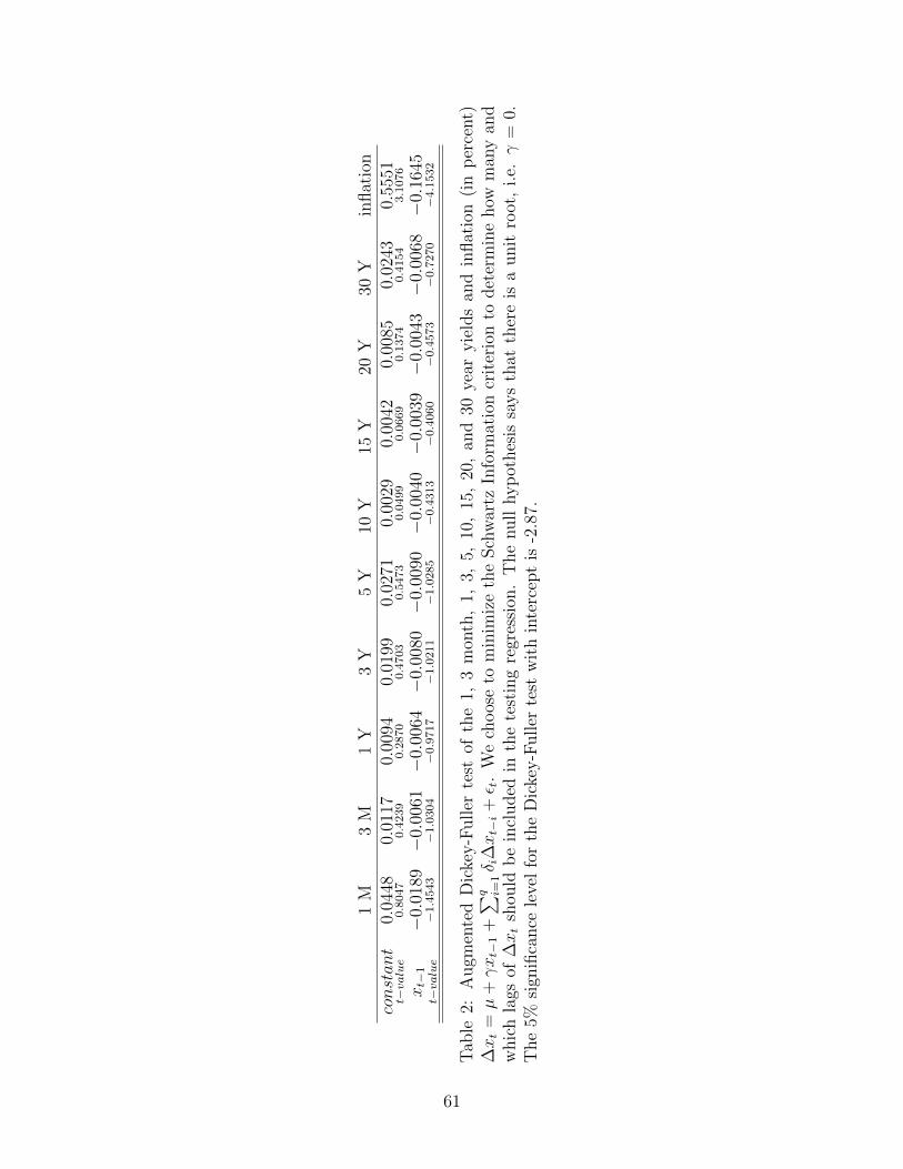
1M

3M

1Y

3Y

5Y

10Y

15Y

20Y

30Y

inflat

ion

constant

t−value

0.04

480.8

047

0.01

170.4

239

0.00

940.2

870

0.01

990.4

703

0.02

710.5

473

0.00

290.0

499

0.00

420.0

669

0.00

850.1

374

0.02

430.4

154

0.55

513.1

076

xt−

1t−value

−0.

0189

−1.4

543−

0.00

61−

1.0

304−

0.00

64−

0.9

717−

0.00

80−

1.0

211−

0.00

90−

1.0

285−

0.00

40−

0.4

313−

0.00

39−

0.4

060−

0.00

43−

0.4

573−

0.00

68−

0.7

270−

0.16

45−

4.1

532

Tab

le2:

Augm

ente

dD

icke

y-F

uller

test

ofth

e1,

3m

onth

,1,

3,5,

10,

15,

20,

and

30ye

aryie

lds

and

inflat

ion

(in

per

cent)

∆xt

=µ

+γxt−

1+∑ q i=

1δ i

∆xt−i+ε t

.W

ech

oos

eto

min

imiz

eth

eSch

war

tzIn

form

atio

ncr

iter

ion

todet

erm

ine

how

man

yan

dw

hic

hla

gsof

∆xt

shou

ldb

ein

cluded

inth

ete

stin

gre

gres

sion

.T

he

null

hyp

othes

issa

ys

that

ther

eis

aunit

root

,i.e.γ

=0.

The

5%si

gnifi

cance

leve

lfo

rth

eD

icke

y-F

uller

test

wit

hin

terc

ept

is-2

.87.

61

1 M 3 M 1 Y 3 Y 5 Y 10 Y 15 Y 20 Y 30 Y inflationd

std.err.0.16800.1297

0.27540.0613

0.22310.0645

0.17280.0682

0.15450.0786

0.10480.0924

0.10940.1026

0.12910.0928

0.16330.0779

0.34740.0357

Table 3: Estimates of the long memory parameter d based on the parametric estimator ofARFIMA(1, d, 1) process based on Chan and Palma (1998) estimator. The standard errorsare reported in small font.

ψx θx dx ψz θz dz0.89920.0010

0.58770.0136

0.28620.0032

0.86980.0014

0.98570.0156

0.18780.0021

µr σx σz σπ0.00590.0016

0.00550.0001

0.00030.0001

0.03130.0013

λx0 λz0 βzx δz×1000 ×100

−0.02950.0008

−2.88800.0414

0.00180.0001

−0.01920.0006

λx1 λx2 λz1 λz2×100000

0.00080.0001

0.26730.0019

−0.02910.0001

−2.57230.0463

σ1 σ3 σ12 σ36 σ60

0.00620.0001

0.00380.0002

0.00300.0002

0.00070.0002

0.00090.0002

σ120 σ180 σ240 σ360

0.00070.0003

0.00040.0001

0.00110.0004

0.00330.0001

Table 4: Estimates of the model with 2-long memory factors. The standard errors arereported in small font. The model is estimated by the approximate maximum likelihoodestimator proposed by Chan and Palma (1998) with the truncation lag set to 60. Thesample period is 1986:01 to 2011:12.

62

ψx θx dx ψz θz dz0.97590.0037

0.30260.0427

− 0.96370.0021

0.82640.0282

−µr σx σz σπ

0.02060.0013

0.00180.0002

0.00080.0001

0.03240.0017

λx0 λz0 βzx δz×1000 ×100

−0.18300.0010

−0.33290.0424

−0.00340.0001

0.03060.0048

λx1 λx2 λz1 λz2×100000

−0.03990.0001

−0.11360.0009

−0.01210.0011

−0.25550.0142

σ1 σ3 σ12 σ36 σ60

0.00680.0004

0.00420.0003

0.00270.0002

0.00070.0004

0.00070.0001

σ120 σ180 σ240 σ360

0.00100.0016

0.00090.0014

0.00150.0010

0.00460.0011

Table 5: Estimates of the model with two short memory factors. The long memory param-eters are suppressed to zero. The standard errors are reported in small font. The model isestimated by the approximate maximum likelihood estimator proposed by Chan and Palma(1998) with the truncation lag set to 60. The sample period is 1986:01 to 2011:12.

Regressand:PC1 PC2 PC3 PC4

Regressor:x 0.9617 0.0263 0.0024 0.0001z 0.9468 0.0446 0.0001 0.0003

x and z 0.9920 0.9243 0.0112 0.0010

Table 6: The sample period is 1986:01 to 2011:12.

Maturity 1 M 3 M 1 Y 3 Y 5 Y 10 Y 15 Y 20 Y 30 YMean 1.1385 1.1288 1.1047 1.2610 1.5438 2.3205 2.9885 3.5793 4.6126Std Dev 2.2422 2.2539 2.2090 1.9465 1.7139 1.4410 1.3396 1.3443 1.4181Skew −0.3969 −0.3935 −0.3959 −0.3458 −0.1970 0.0370 0.1151 0.1208 0.2541Ex. Kurtosis −0.7528 −0.7584 −0.7588 −0.8080 −0.9382 −0.9897 −0.9680 −1.0480 −1.1438Min −3.4420 −3.5061 −3.5324 −2.7312 −1.8234 −0.7674 0.0016 0.6025 1.7792Max 5.7061 5.8617 5.8025 5.1860 4.9165 5.1039 5.7504 6.4154 7.75251st lag Autocorr. 0.9579 0.9539 0.9469 0.9458 0.9445 0.9384 0.9336 0.9340 0.939112th lag Autocorr. 0.7412 0.7418 0.7507 0.7827 0.8037 0.8186 0.8208 0.8277 0.840324th lag Autocorr. 0.3779 0.3860 0.4296 0.5299 0.6062 0.6857 0.7166 0.7370 0.7524

Table 7: Descriptive statistics for the real yields implied by the model (in percent). Thesample period is 1986:01 to 2011:12.

63

Panel A: value of the log-likelihood function:model LM SMlog − likelihood 13549 13323

Panel B: likelihood ratio test:LR

p−value252

0

Table 8: Panel A - Log-likelihood value of particular model specification: LM - model withtwo lond memory factors, and SM - model with two short memory factors. In the restrictedmodels the long memory parameters were supressed to zero and reestimated. Panel B -likelihood ratio test of the null hypothesis about lack of short memory in two factors, SM.Thus, the restrictions are tested against the alternative with two long memory factors (fullmodel). In small font is given the p-value (the critical value at the 5 percent confidence levelis 5.99). The distribution of the test is Chi-square with one and two degrees of freedom forthe LMI and SM models, respectively.

overall 1 M 3 M 1 Y 3 Y 5 Y 10 Y 15 Y 20 Y 30 YLM 29.38 64.91 38.40 27.69 4.51 7.48 6.72 1.91 9.98 33.04SM 32.88 69.63 42.71 25.45 4.14 5.55 8.66 6.81 14.41 45.11

Table 9: In sample fit root mean square error (RMSE) for particular maturities and overallfor LM and SM models. The fitted values are found by applying the Kalman filter. Thestatistics are reported in percentage. The sample period is 1986:01 to 2011:12.

yield 1 M 3 M 1 Y 3 Y 5 Yforecast horizon Panel A − LM specification

1 M 24.66 23.56 37.79 57.92 33.103 M 55.65 59.50 76.93 91.60 62.976 M 101.91 106.36 121.07 129.84 94.831 Y 180.29 183.80 188.78 176.82 127.06

Panel C − SM specification1 M 26.30 25.45 37.12 48.88 34.073 M 61.91 64.98 75.41 86.01 67.496 M 113.34 116.41 124.34 129.53 105.891 Y 195.70 197.37 195.82 187.22 151.71

Table 10: Root Mean Square Error of in-sample forcasting power of particular models: longmemory (LM) in panel A, long memory in inflation only (LMI) in panel B, and short memory(SM) in panel C. The statistics are reported for different forecasting horizons: 1, 3, 6 and12 months. For calculation of the forecast errors we use the last 10 years of the sample.Using the parameter estimates obtained from the full sample we start forecasts in 2000:12for the four horizons. We obtain 120 forecasts for 1 month horizon, 118 forecasts for 3 monthhorizon, 115 forecasts for 6 month horizon, and 109 forecasts for 12 month horizon. Theforecasts are obtained by using the Kalman filter. The smallest RMSE among the modelshighlighted in bold font. The statistics are reported in basis points.

64

yield 1 M 3 M 1 Y 3 Y 5 Yforecast horizon Panel A: LM specification

1 M 30.88 24.03 47.51 80.02 32.593 M 54.05 60.10 88.37 111.76 61.116 M 106.00 113.60 139.57 149.62 90.381 Y 197.15 202.99 215.11 196.43 118.26

Panel C: SM specification1 M 28.57 24.57 34.95 51.75 36.463 M 62.41 67.29 82.13 97.06 77.176 M 124.09 129.55 142.73 152.02 126.611 Y 223.41 226.94 230.98 227.21 190.72

Panel D: AP specification1 M 51.37 41.69 29.91 40.86 32.003 M 105.41 89.21 68.75 74.94 59.106 M 149.05 133.08 110.92 105.11 87.221 Y 201.37 192.50 167.61 143.34 109.90

Panel E: ABW specification1 M 33.85 45.35 85.32 72.41 30.923 M 68.46 82.32 111.57 90.61 54.606 M 111.58 121.53 137.27 107.98 74.961 Y 162.07 165.73 161.18 117.75 88.08

Panel F: DL specification1 M 35.43 28.19 24.88 35.68 32.763 M 63.18 59.98 58.78 70.22 62.246 M 100.79 99.73 101.80 108.33 94.041 Y 158.57 159.50 158.36 148.88 118.49

Panel G: RW specification1 M 29.29 22.60 23.36 29.72 31.053 M 49.66 47.25 49.31 55.55 54.836 M 83.62 80.30 79.62 80.38 77.551 Y 148.44 145.84 133.79 110.60 91.49

Table 11: Root Mean Square Error of out-sample forcasting power of particular models: longmemory (LM) in panel A, and short memory (SM) in panel B. The out-of-sample forecasterrors are calculated by rolling widow estimation of the model (607 observations), based onthe last 5 years of the sample. In the first step we estimate the model using the period1952:06 to 2000:12, and using the Kalman filter make predictions for 4 different horizons.In the second step we estimate the model using the period 1952:07 to 2001:01. We repeatthe procedure 120 times. We obtain 120 forecasts for 1 month horizon, 118 forecasts for 3month horizon, 115 forecasts for 6 month horizon, and 109 forecasts for 12 month horizon.The statistics are reported for different forecasting horizons: 1, 3, 6 and 12 months. Thesmallest RMSE among the models highlighted in bold font. The statistics are reported inbasis points.

65

long memory a ne term structure models - usi - eco · long memory a ne term structure models adam...

Documents