long range trends in adult mortality: models and
TRANSCRIPT

1
LONG RANGE TRENDS IN ADULT MORTALITY: MODELS AND PROJECTION
METHODS
John Bongaarts
Population Council
1 Dag Hammarskjold Plaza
New York, NY, 10017
Abstract
This study has two objectives: (1) to test a new model for the pattern of change over time
in age-specific adult mortality rates, and (2) to develop a new methodology for projecting
future trends in adult mortality. The first part of the paper presents a test of the goodness-
of-fit of the logistic model for the force of mortality using data from the Human Mortality
Data Bank for females and males aged 25-109 in 14 populations. The results from this
exercise suggest a new version of the logistic model which is called the shifting logistic
model, because the senescent mortality function is assumed to shift to higher ages over
time. This approach contrasts with the conventional view that mortality declines as adult
life expectancy rises. The last part of the paper proposes a new projection method based
on the shifting mortality model. This method is compared with the widely used Lee-
Carter procedure.
Paper prepared for the Session on Mathematical Demography at the Annual Meeting of
the Population Association of America, Boston, 1-3 April 2004

2
Over the past two centuries life expectancy at birth in the industrialized ("developed")
world approximately doubled, reaching 79 years for females and 72 years for males in
2000-2005 (United Nations, 2002). Much of this rise is attributable to large reductions in
infant and child mortality. Mortality among the young is now so low, however, that
further declines will have little impact on future trends in life expectancy. Future
increases in life expectancy will therefore require additional reductions in adult mortality.
This study will examine past trends in the age pattern of adult mortality and discuss their
implications for long range mortality projections.
The description of observed age patterns of adult mortality with mathematical models is
one of the oldest and most important topics in demography. The number and complexity
of mortality models have grown rapidly since Gompertz proposed the first “law of
mortality” in 1825. These developments have been made possible by the increasing
availability of detailed mortality statistics in many countries. A good model provides a
simple but adequate mathematical description of mortality by age and/or time. The
objective is to identify fundamental and persistent patterns in the data and summarize
them with as few parameters as possible. Models have found many uses, including
smoothing of data, construction of model life tables, comparative analyses, testing of
theories and forecasting (Keyfitz, 1984; Tabeau et. al., 2001).
A concise model description of past mortality trends provides the basis for projections.
The theory and practice of forecasting mortality have evolved rapidly in recent decades
and there are many ways to make forecasts (Keyfitz, 1991; Lee, 1998; Olshansky, 1988;
Pollard, 1987; Tabeau et al., 2001). Projections for the short run typically rely on simple
extrapolation of historical trends in mortality rates, in life expectancy or in model
parameters. However, in projections for periods of more than a few decades, simple
linear extrapolation can lead to implausible results and expert judgment is then often used
to decide which long-range levels or trends are most probable. For example, experts may
identify a target for life expectancy at birth in a future year. This has been the approach
used by the United Nations, the World Bank and many national statistical agencies to
make long-range population projections.
This study has two overall objectives: (1) to test a new model to describe the pattern of
change over time in age-specific adult mortality rates, and (2) to develop a new
methodology for projecting future trends in adult mortality. The first section of the paper
presents a brief overview of models for the age pattern of adult mortality and a test of the
goodness-of-fit of the logistic model for the force of mortality. This test uses data from
the Human Mortality Data Bank for females and males aged 25-109 in 14 populations.
The results of this exercise suggest a new version of the logistic model which will be
called the shifting logistic model, because the adult mortality function is assumed to shift
to higher ages over time. The second part of the paper applies this new model to
decompose the rate of change in the force of mortality schedule into “background” and
“senescent” components. This analysis provides crucial insights into the assumptions
made by projection methods that rely on extrapolation of the rate of mortality
improvement. The final section proposes a new projection methodology based on the

3
shifting mortality model. The new method is compared with the Lee-Carter procedure
which is one of the most widely used methods for projecting mortality.
I. Models for the force of mortality a) Age pattern
Mortality rates in a wide range of populations show an approximately exponential rise
with age for adults. A simple parametric model proposed by Gompertz (1825)
summarizes this pattern:
xex βαµ =)( , (1)
where )(xµ denotes the force of mortality at age x . The two parameters α and β are
positive; α varies with the level of mortality and β measures the rate of increase in
mortality with age.
For many purposes the Gompertz model provides a satisfactory fit to adult mortality
rates. However, close inspection of the difference between model estimates and observed
death rates often reveals systematic underestimation of actual mortality at youngest adult
ages (under 40) and overestimation at the oldest ages (over 80). The deviation at lower
ages is addressed by Makeham (1860) with the addition of a constant to the Gompertz
model
γαµ β += xex)( (2)
The new parameter γ is usually referred to as background mortality which is the same for
all ages. A detailed analysis of (2) is provided by Gavrilov and Gavrilova (1991).
The Makeham model represents a clear improvement over the Gompertz model at
younger ages, but it still overestimates mortality at the oldest ages. This deviation can be
addressed in a number of ways, most simply by the following logistic model (Thatcher,
1999, Thatcher et al.,1998) :
γα
αµ β
β
++
=x
x
e
ex
1)( (3)
At lower adult ages the force of mortality estimated with models (3) and (2) are very
similar, because the denominator of the first term in (3) is close to 1. At the oldest ages,
however, the two models diverge as (3) levels off at 1+ γ while (2) has no limit.
More complex logistic models with additional parameters have also been proposed
(Beard, 1971; Horiuchi and Wilmoth, 1998; Perks, 1932; Thatcher et al., 1998). Based on
a detailed comparison of different models Thatcher (1999) and Thatcher et al. (1998)
recommend (3) because it provides an excellent fit to mortality rates over the entire adult
age range with relatively few parameters.

4
The good fit of the logistic model (3) is demonstrated in Figure 1 which presents
observed and estimated values of )(xµ for Swedish females in 1875, 1950 and 2000. The
proportion of the variance explained by the model equals 0.9997 in 1875, 0.9996 in 1950
and 0.9985 in 2000.
To confirm these results for other populations the model given by (3) was fitted to annual
mortality data from 1950 to 2000 for 14 countries, separately for males and females. All
countries in the Human Mortality Databank outside Eastern European were included:
Austria, Canada, Denmark, England and Wales, Finland, France, Italy, Japan,
Netherlands, Norway, Sweden, Switzerland, USA, West Germany. Table 1 presents
averages of annual estimates for α, β and γ for females and males in each of the 14
countries for all available years 1950-2000.1 These results are discussed further below but
for now it should be noted that the model fits very well in all these countries (see next to
last column in Table 1). The fit is about the same for females (R2 averages 0.9993 for the
14 countries) as for males (R2 averages 0.9996).
Although the simple logistic model is well suited for present purposes, its fit is not
perfect. An examination of differences between observed and fitted values reveals small
systematic overestimation of mortality between ages 60 and 80, as well as some
underestimation at the highest ages among females in a number of countries. This pattern
is consistent with the findings of Himes et al. (1994).
In the following analysis of trends in adult mortality it is useful to distinguish between
senescent mortality which rises with age and background mortality which does not vary
with age (Gavrilov and Gavrilova, 1991, Horiuchi and Wilmoth, 1998, Makeham, 1860).
The sum of these two components equals the force of mortality:
( , ) ( , ) ( )s bx t x t tµ µ µ= + (4)
where ( , )s x tµ = senescent force of mortality
( )b tµ = background force of mortality
For the logistic model the first term on the right hand side of (3) equals ( , )s x tµ and
( ) ( )b t tµ γ= .
Figure 2 plots model estimates of these two components for Swedish females in 1875,
1950 and 2000. The senescent component rises linearly from age 25 to about age 75,
because in this age range the denominator of the senescent component of (3) is close to
1.0, and the remaining exponential term in the numerator becomes a straight line when
plotted on a logarithmic scale as is the case in Figure 2. At ages above about 75 the rate
of increase in the force of mortality with age declines in the logistic model and at very
high ages ),( txsµ approaches 1.0. The age invariant background component (plotted as
horizontal lines in Figure 2) has declined sharply over time from 0.00740 in 1875 to
0.00078 in 1950 and to 0.00013 in 2000. The senescent and background components in
Figure 2 add up in each year to the overall model estimate of the force of mortality

5
plotted in Figure 1. At high ages background mortality is small compared to senescent
mortality and it may be ignored for many analytic purposes, especially in contemporary
countries with high life expectancy.
b) Trend over time
Trends in adult mortality can be summarized with time series of the three parameters α(t),
β(t) and γ(t). Figures 3a-c present estimated trends in these parameters for each of the 14
countries from 1950 to 2000. Several conclusions can be drawn from these results. There
is considerable variation among countries in α(t), but the trend in this level parameter is
typically downward. The same is true for background mortality γ(t) (see Figure 3c) but
there is less variation among countries in γ(t) than in α(t). In addition, declines in γ(t) are
mostly confined to the period 1950 to 1975. After 1975 there appears to be little
systematic trend in γ(t) in many of these countries, suggesting that background mortality
has reached a low level plateau.
The most interesting finding in Figure 3b is that values of β(t) are nearly constant for
each population. Similar patterns are observed for males (data not shown). This finding
confirms earlier observations by Gavrilov and Gavrilova (1991) and Thatcher (1999). In
fact, the near constancy of β(t) extends further into the past. For example, for Swedish
females β(t) averaged 0.118 for 1875-1900, 0.119 for 1900-1950 and 0.117 for 1950-
2000.
This conclusion about the lack of variation with time in β(t) is confirmed in Table 1
which presents averages of annual estimates of the coefficients of variation in α(t), β(t)
and γ(t) for females and males in 14 countries for the period 1950-2000. The coefficient
of variation of β(t) is small, averaging just 2.2 percent for females and 3.0 percent for
males. In contrast, the coefficients of variation for α(t),and γ(t) are at least an order of
magnitude larger for both males and females. Clearly, α(t),and γ(t) are much more
variable than β(t).
c. Shifting logistic model
The finding that β(t) is nearly constant suggests a variant of the logistic model in which
this parameter is assumed fixed over time for a population. The senescent component of
the standard model (3) then simplifies to
x
x
set
ettx
β
β
αα
µ)(1
)(),(
+= (5)
in which α(t) is the only time varying parameter. The value of β can differ among
populations and may take different values for males and females, but it is constant with
respect to time.
A change in the senescent force of mortality from 0( , )s x tµ at time 0t to ( , )s x tµ at time t
is conventionally interpreted as a rise or decline in mortality rates. Formula (5) offers an
alternative and unconventional description of changes in the force of mortality. Instead of
interpreting mortality as rising or falling over time, the schedule of the force of senescent

6
mortality can be viewed as shifting to higher or lower ages. This interpretation is possible
because (5) has an interesting and very useful property: the age pattern ),( txsµ at time t is
the same as at an earlier time t0 except that the function has shifted to higher (lower) ages
as senescent mortality falls (rises). The force of mortality at age x in year t is identical to
the value of the force of mortality in an earlier year t0 at age x-S(t) except around age
zero. As a result, (5) can be written as
( ( ))
0
( ( ))
0
( )( , )
1 ( )
x S t
s x S t
t ex t
t e
β
β
αµ
α
−
−=
+ (6)
where S(t) equals the amount of the shift in years up or down the age axis between t0 and t
(equation (6) holds for x>S(t), and ( , ) 0s x tµ = for x<S(t)). As shown in Appendix A, the
conventional up-down and the alternative shifting interpretations are formally equivalent
for the logistic model with
0ln( ( ) / ( ))( )
t tS t
α αβ
= − (7)
That is, a change in the senescent force of mortality between 0t and t can be described
with (5) as a change in the level parameter 0( )tα to ( )tα or equivalently with (6) as a
shift by S(t) years.
The idea of a shifting mortality schedule can be clarified further by introducing the
senescent life expectancy at birth denoted es(t) and defined as
addxtxtea
ss ∫∞
∫−=0 0
),(exp)( µ (8)
It equals the average age at death of a newborn subjected to ),( txsµ , assuming no
background mortality and no non-senescent mortality at younger ages. The shift to higher
or lower ages in the force of senescent mortality function between t0 and t is closely
approximated by the change in senescent life expectancy between t0 and t:
0( ) ( ) ( )s sS t e t e t≈ − (9)
because ( , )s x tµ is very small around age zero.
The pattern of ),( txsµ given by (6) will be referred to as the shifting logistic model . It is
a member of a more general class of models for which the shifting assumption holds with
0( , ) ( ( ), )s sx t x S t tµ µ= − (10)
The shifting logistic model (6) always implies (10) but the shifting assumption given by
(10) may hold even when ),( txsµ does not follow a logistic (more on this below). It
should be emphasized that, in general, the shifting property applies only to senescent
mortality and not to all adult mortality.

7
The shifting is evident in Figure 2 where the lines for senescent mortality in 1875, 1950
and 2000 have similar shapes with the schedules for later years moved to higher ages
compared to earlier years. The shift equaled 3 years between 1875 and 1950 and 7 years
between 1950 and 2000. A shifting pattern for mortality change was proposed earlier by
Kanisto et al. (1996) and some of its implications are examined by Bongaarts and Feeney
(2002, 2003).
The shifting logistic model describes changes over time in the age pattern of senescent
mortality with only one time varying parameter, S(t). This advantage is offset by some
loss in the goodness-of-fit. However, the proportion of variance explained by the shifting
model with constant β is still an impressive 0.9993 for females and 0.9995 for males
(average of 14 populations and all years from 1950 to 1999). The last column of Table 1
presents the R2 values for males and females in each of the 14 countries with β held
constant at its average for 1950-2000. These results are only slightly smaller than the R2
for the logistic model with a variable β(t) presented in the next to last column in Table 1.
These results indicate that the shifting logistic model provides a good general description
of age patterns of adult mortality in many countries for the past half century. The next
sections of this study examine the implications of this new model.
II. Models for the rate of change in the force of mortality Past studies of mortality trends have gained important insights by examining the rate of
change in the force of mortality with respect to age or time (Horiuchi and Coale, 1990,
Horiuchi and Wilmoth, 1998; Keyfitz, 1977; Vaupel, 1986; Vaupel and Romo, 2003). A
discussion of this topic is essential to understanding the factors that drive change in adult
mortality, to the evaluation of existing projection methods and to the development of a
new projection procedure.
a) Rate of change by age
The relative derivative of ( , )x tµ with respect to age is defined as
1 ( , )
( , )( , )
x tk x t
x t x
µµ
∂=
∂ (11)
and is referred to as the age-specific rate of mortality change with age (Horiuchi and
Coale, 1990) or the life table aging rate (Horiuchi and Wilmoth, 1998).
Figure 4a plots observed and model estimated values of ),( txk for Swedish females in
1875, 1950 and 2000. The pattern is bell-shaped and varies over time. It is also somewhat
different for males than for females (data not shown).
To interpret these changes with age and over time it is useful to decompose ),( txk into
two additive factors representing, respectively, the senescent component ),( txks and the
background component ),( txkb (see Horiuchi and Wilmoth, 1998, for a slightly different
decomposition):

8
),(),(),( txktxktxk bs += (12)
The senescent component ),( txks is defined as the aging rate that would be observed in
the absence of background mortality and ),( txkb equals the difference between ),( txk and
),( txks .
As shown in Appendix B, for the shifting logistic model
( , ) [1 ( , )]1 ( )
s sxk x t x t
t eββ
β µα
= = −+
(13)
xb
etttxk βαγ
β)()](/11[1
),(++
−= (14)
Figure 4b plots the model senescent component ),( txks for Swedish females in 1875,
1950 and 2000. At the youngest ages ),( txks is approximately constant and equal to β
because ( , ) 1s x tµ << . With advancing age ),( txks declines and reaches 0 at very high
ages. The schedules for ),( txks and ( , )s x tµ shift together to higher (lower) ages as
senescent life expectancy rises (falls).
Figure 4c plots model estimates of the background component ),( txkb for Swedish
females in 1875, 1950 and 2000. The value of ),( txkb is negative and rises from - β at
very young ages to 0 at the oldest ages. An interesting property of the ),( txkb schedule is
that it shifts to higher/lower ages. But, in general, this shifting occurs at a different rate
from the shifting in ),( txsµ and ),( txks . In most countries ),( txkb either moves slower
to the right than ),( txks (when γ(t) declines but less rapidly then α(t)) or it shifts to the
left (when γ(t) declines more rapidly then α(t)). For Swedish females the background
component has clearly moved to the left between 1875 and 1950 and again between 1950
and 2000 due to a very rapid decline in background mortality.
The background and senescent components combine to produce the overall pattern of
),( txk as shown in Figure 4d for Swedish females in 1950. In general, shifts over time of
the ascending portion of the bell shape at lower ages are attributable to shifts in the
background component ),( txkb , and shifts in the descending portion of the bell at higher
ages are caused by shifts in the senescent component ),( txks (see related discussion in
Horiuchi and Wilmoth, 1998). As a result, the overall bell shaped pattern for
),( txk exhibits complex changes and can move to the left or right and become wider or
narrower depending on trends in ),( txks and ),( txkb which in turn are determined by α(t),
β and γ(t). This makes it difficult to draw conclusions about trends in senescent mortality

9
from the overall shape of ),( txk . It is therefore preferable to analyze the background and
senescent components separately or to limit the analysis to highest ages where senescent
mortality dominates.
b) Rate of change over time
The relative derivative of the force of mortality with respect to time is defined as
1 ( , )
( , )( , )
x tx t
x t t
µρ
µ∂
= −∂
(15)
and is called the rate of improvement in mortality (Keyfitz, 1977; Vaupel, 1986; Vaupel
and Romo, 2003).
Annual estimates for ),( txρ tend to fluctuate widely and the empirical analysis of this
variable is therefore usually restricted to averages over periods of one or more decades.
Figure 5a plots observed and model estimated values of ),( txρ for Swedish females from
1875 to 1950 and from 1950 to 2000. For both periods ),( txρ declined with age. To
interpret these changes with age and over time it is again useful to decompose ),( txρ into
two additive factors, the senescent component ),( txsρ and the background component
),( txbρ :
),(),(),( txtxtx bs ρρρ += (16)
The senescent component ),( txsρ is defined as the rate of mortality improvement that
would be observed in the absence of background mortality and ),( txbρ equals the
difference between ),( txρ and ( , )s x tρ .
As shown in Appendix C, if the shifting assumption (10) holds, then
( , ) ( ) ( , )s s sx t e t k x tρ = & (17)
1 ( )
( , ) ( ) ( , )( , )
bb s b
d tx t e t k x t
x t dt
µρ
µ= −& (18)
Where )(tes& denotes the derivative of senescent life expectancy with respect to time:
( ) ( ) /s se t de t dt=& . Note that (17) and (18) are valid even if senescent mortality does not
follow the logistic, provided the shifting assumption holds. If the shifting logistic model
applies, substitution of (13) in (17) gives
( , ) ( ) [1 ( , )]s s sx t e t x tρ β µ= −& (19)
and γ(t) can be substituted for ( )b tµ in (18). Equation (19) is a more general version of
the formula ( ) ( )s st e tρ β= & derived by Vaupel (1986) for the Gompertz model. (Note also
that when background mortality is constant, ( , ) ( ) ( , )sx t e t k x tρ = & ).

10
Figure 5b plots model estimates of ),( txsρ obtained from (19) for Swedish females from
1875 to 1950 and from 1950 to 2000. The age pattern of ),( txsρ (but not its level) is the
same as for ),( txks : at the lowest ages ),( txsρ is constant with age, equal to )(tes&β ,
because ( , ) 1s x tµ << . With advancing age ),( txsρ declines and reaches 0 at very high
ages following the same pattern of relative decline as ),( txks . The level of ),( txsρ is
substantially higher for 1950-2000 than for 1875-1950 because senescent life expectancy
rose at a more rapid pace in the former than in the latter period. The schedule for ),( txsρ
shifts to the right as senescent life expectancy rises, as was the case for ),( txks and
( , )s x tµ .Variations in the schedule ),( txsρ over time and with age are therefore the net
result of two factors: (1) up/down movements over time due to variation in )(tes& and (2)
shifts to higher (lower) ages as ( )se t rises (falls).
Model estimates of the background component of the rate of mortality improvement for
Swedish females from 1875 to 1950 and from 1950 to 2000 are plotted in Figure 5c. Over
these two periods the decline in background mortality has been rapid and the second term
on the right-hand side of (18) has dominated. This term is directly proportional to the rate
of change in background mortality and since γ(t) has declined over time (i.e., its
derivative is negative) ( , )b x tρ has been positive, as is evident in Figure 5c. The more
rapidly γ(t) declines, the more positive ( , )b x tρ becomes. In addition, ( , )b x tρ declines
sharply with age and approaches zero at high ages. (Note that ( , )b x tρ is negative when
background mortality is constant and senescent life expectancy is rising, because
( , )bk x t is negative.)
The senescent and background components combine to produce the patterns of change in
the overall rate of improvement in mortality ),( txρ as illustrated in Figure 5d for Swedish
females for the period 1950-2000. Below about age 70 the decline in ),( txρ with age is
attributable to a decline in the background component while the senescent component is
approximately constant at )(tes&β . At ages above 70, ),( txbρ is near zero and ),( txsρ
declines, reaching zero at very old ages.
The pattern of ),( txρ varies widely over time and among countries as shown in Figure
6a-d which compares model estimates of ( , )x tρ for 1950-1960 and 1985-1995 for
England and Wales, France, Italy and Japan. To facilitate the interpretation of these
results the values of )(tes&β for 1950-1960 and 1985-1995 are plotted as horizontal
dashed lines. In the middle adult ages (around age 70) ( , )x tρ is close to this line. At
younger ages ( , )x tρ is either above (1950-1960) or below (1985-1995) this line
depending largely on the rate of decline in γ(t). At older ages ( , )x tρ declines with age and
shifts to higher ages as senescent life expectancy rises.

11
Given the complexity of changes in ( , )x tρ it is difficult to draw conclusions from them
about overall trends in adult mortality. As was the case for ),( txk it is preferable to
analyze the background and senescent components of ( , )x tρ separately. Limiting the
analysis to highest ages where the senescent component dominates is somewhat helpful,
but it is difficult to determine whether changes at the highest ages are due to shifting
(caused by a change in the level of senescent life expectancy) or by an up or down
movement (caused by variation in the rate of change in senescent life expectancy).
This analysis of the rate of change in the force of mortality leads to two conclusions.
First, the age pattern of ),( txρ has changed substantially in recent decades in many
countries. This makes it likely that the rate of mortality improvement will not be constant
in the future as assumed in the Lee-Carter projection method. Second, the factors
responsible for the variation in ),( txρ include different trends in background and
senescent mortality and the shifting of the pattern of senescent mortality. These findings
have implications for projection methods as discussed next.
III. Projecting mortality rates
The models for the force of mortality discussed in the preceding sections will now be
applied to gain insights into projection methods. After a brief description of the Lee-
Carter method, a new forecasting approach will be proposed.
a) The Lee-Carter method
Lee and Carter (1992) proposed a new statistical method for modeling and
forecasting mortality by age which has been adopted widely. For example, the US Census
Bureau uses the Lee-Carter forecast as a benchmark for their long-run forecast of life
expectancy (Hollman et. al., 2000) and a Social Security Technical Advisory Panel
recommended the adoption of the method (Technical Panel on Assumptions and
Methods, 1999; Lee and Miller, 2001). Projections of mortality for the G7 countries by
Tuljapurkar et. al., (2000) also use this method. Based on the recommendations of an
expert group, the United Nations Population Division has prepared its long-range
projections to 2300 for all countries in the world with a variant of the Lee-Carter model
(United Nations, 2003). Recent discussion of the model and its applications can be found
in Lee (1998), Lee (2000), Lee and Miller (2001), Booth et. al. (2002), Carter and
Prskawetz (2003) and Tabeau et. al. (2001).
The Lee-Carter method is based on the following mortality model:
),()()()()],(ln[ txtkxbxatxm ε++= (20)
where
m(x,t) = central death rate at age x and time t
k(t) = index of level of mortality
a(x) = age-specific constants describing the general pattern of mortality by age
b(x) = age-specific constants for the relative speed of mortality change
ε(x,t) = residual
12
This model provides a good fit to past age-specific mortality rates in the US, explaining
93 percent of the within age group variance between 1900 and 1987 (Lee and Carter,
1992).
Equation (20) provides the basis for making mortality projections. A projection requires
only the extrapolation of the index k(t), because a(x) and b(x) are estimated from past
data and are held constant for the duration of the projection. An ARIMA time series
model is usually used for k(t), and Lee and Carter (1992) and other analysts have
assumed a random walk with a drift which describes past trends in k(t) well. The
implication of assuming a linear trend in k(t) to continue into the future is that mortality
rates at all ages follow an exponential decline. That is, the projected proportional rate of
mortality decline ( , )x tρ in a future year t varies by age but it is assumed to be the same at
each age as the rate observed in the past:
( , ) ( )hx t xρ ρ= (21)
where )(xhρ is the observed rate of decline in the death rate at age x over some historical
period h which ends in the base year of the projection. To insure robust results Lee and
Carter recommend that estimates of )(xhρ be based on historical data for periods of
several decades.
The model has several attractive features: a relatively simple demographic model
captures the main trends in patterns of past mortality change; forecasting is based on
persistent long-term trends and involves no subjective judgment; and the application of
statistical time series methods provides probabilistic confidence intervals for the forecast
(Lee and Miller, 2001; Booth et. al., 2002). In addition, tests in several populations
indicate that projections made with this method are quite accurate over short time
horizons (Lee and Miller, 2001). There are, however, also limitations which become
increasingly significant as the projection duration rises:
(1) A key assumption of the model (that the rate of decline in mortality at each age
remains invariant over time) is violated in several countries in recent decades. Instead of
being constant, rates of mortality improvement have tended to decline over time at
younger ages while rates of improvement have risen at older ages (Booth et. al., 2002;
Carter and Prskawetz, 2003; Lee, 2000; Lee and Miller, 2001). The results presented in
Figures 6a-d also indicate that the age pattern of ( , )x tρ has varied over time.
(2) Forecasts in industrialized countries typically underestimate improvements in life
expectancy (Lee and Miller, 2001). This is presumably due to a tendency to
underestimate mortality improvements at older ages, because errors at young ages have
little effect on projections of life expectancy in populations with low mortality.
(3) Extrapolation of trends in age-sex-specific mortality rates or transformations of these
rates (Lee-Carter use the log of death rates) can result in implausible results if projected
over many decades (Keyfitz, 1984; Lee, 2000; McNown, 1992; Tabeau et al. 2001).
Some investigators have attempted to address these limitations by adding complexity and
additional parameters to the Lee-Carter model (Booth et. al., 2002; Carter and Prskawetz,
2003). The alternative approach proposed next provides a simpler solution.
13
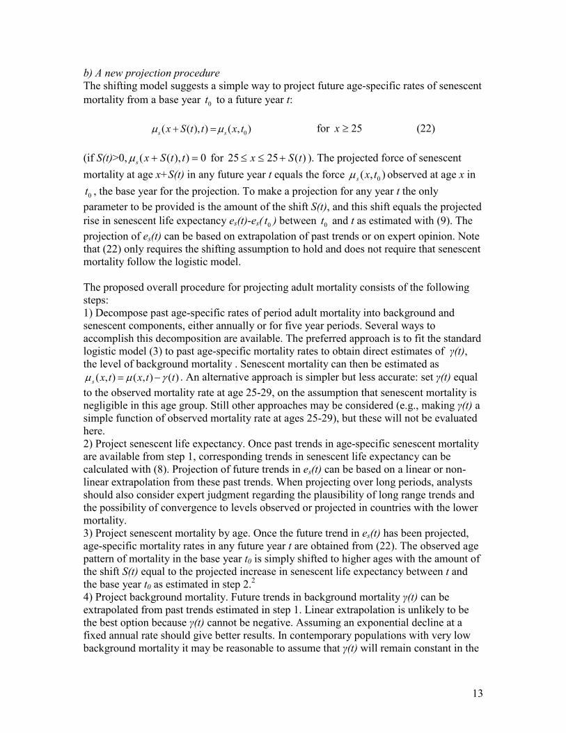
b) A new projection procedure
The shifting model suggests a simple way to project future age-specific rates of senescent
mortality from a base year 0t to a future year t:
0( ( ), ) ( , )s sx S t t x tµ µ+ = for 25x ≥ (22)
(if S(t)>0, ( ( ), ) 0s x S t tµ + = for 25 25 ( )x S t≤ ≤ + ). The projected force of senescent
mortality at age x+S(t) in any future year t equals the force ),( 0txsµ observed at age x in
0t , the base year for the projection. To make a projection for any year t the only
parameter to be provided is the amount of the shift S(t), and this shift equals the projected
rise in senescent life expectancy es(t)-es( 0t ) between 0t and t as estimated with (9). The
projection of es(t) can be based on extrapolation of past trends or on expert opinion. Note
that (22) only requires the shifting assumption to hold and does not require that senescent
mortality follow the logistic model.
The proposed overall procedure for projecting adult mortality consists of the following
steps:
1) Decompose past age-specific rates of period adult mortality into background and
senescent components, either annually or for five year periods. Several ways to
accomplish this decomposition are available. The preferred approach is to fit the standard
logistic model (3) to past age-specific mortality rates to obtain direct estimates of γ(t),
the level of background mortality . Senescent mortality can then be estimated as
)(),(),( ttxtxs γµµ −= . An alternative approach is simpler but less accurate: set γ(t) equal
to the observed mortality rate at age 25-29, on the assumption that senescent mortality is
negligible in this age group. Still other approaches may be considered (e.g., making γ(t) a
simple function of observed mortality rate at ages 25-29), but these will not be evaluated
here.
2) Project senescent life expectancy. Once past trends in age-specific senescent mortality
are available from step 1, corresponding trends in senescent life expectancy can be
calculated with (8). Projection of future trends in es(t) can be based on a linear or non-
linear extrapolation from these past trends. When projecting over long periods, analysts
should also consider expert judgment regarding the plausibility of long range trends and
the possibility of convergence to levels observed or projected in countries with the lower
mortality.
3) Project senescent mortality by age. Once the future trend in es(t) has been projected,
age-specific mortality rates in any future year t are obtained from (22). The observed age
pattern of mortality in the base year t0 is simply shifted to higher ages with the amount of
the shift S(t) equal to the projected increase in senescent life expectancy between t and
the base year t0 as estimated in step 2.2
4) Project background mortality. Future trends in background mortality γ(t) can be
extrapolated from past trends estimated in step 1. Linear extrapolation is unlikely to be
the best option because γ(t) cannot be negative. Assuming an exponential decline at a
fixed annual rate should give better results. In contemporary populations with very low
background mortality it may be reasonable to assume that γ(t) will remain constant in the

14
future. Several other options (nonlinear trend, approach to a minimum threshold) may be
considered.
5) Combine the projections of senescent and background mortality to obtain the overall
schedule of adult mortality rates for the duration of the projection. (No attempt will be
made to improve on existing methods for projecting mortality under age 25.
Conventional methods should be adequate, in particular for countries with high life
expectancy because infant and child mortality have reached very low levels and will have
little effect on future trends in overall life expectancy).
Figure 7 presents an illustrative application of this procedure for Swedish females. The
base year is 2000 and future background mortality is held constant at the level observed
in 2000. Two projections are presented with senescent life expectancy rising by 10 and
20 years respectively. The shifting pattern of senescent mortality is evident in Figure 7.
No attempt will made here to forecast the year in which these increases in life expectancy
are likely to be observed, because linear extrapolation of past trends is potentially
problematic and expert opinion should preferably be used for long range projections.
However, if the trend in senescent life expectancy is extrapolated linearly from 1950-
2000 into the future then a ten year rise will be attained in 2072 and a 20 year rise in
2144.
The new method can also be applied in populations for which mortality data are only
available for a single year or period. This is the case for many developing countries
where mortality data are often limited. The available information for one year or period
provides the baseline estimates of levels of background and senescent mortality. The age
pattern of senescent mortality in the base year is then shifted in the projection, but
analysts will have to make assumptions about future trends in background mortality and
senescent life expectancy.
c) Comparison with Lee-Carter methodology
The new projection method partially addressed the weaknesses in the Lee-Carter method:
a) Variations over time in the age-specific rate of decline of mortality. Lee and Carter
(1992) assume the rate of decline in mortality ),( txρ projected for age x in some future
year t to be constant and equal to the average rate observed in some past period. In
contrast, the new method allows this age pattern to change over time by projecting
separate trends for background and senescent mortality. As discussed earlier, different
trends in background and senescent mortality are a key cause of the changing age pattern
of ),( txρ over time. In addition, senescent mortality is allowed to shift to higher ages (see
next point).
b) Underprojection of improvements in life expectancy. As noted, this is probably in part
due to a tendency to underestimate improvements in mortality at older ages. This
tendency is not surprising because Lee and Carter (1992) do not take into account the
shifting of ),( txsµ and ),( txsρ to higher ages that is explicitly built into the new method.
This factor is crucial in long range projections at older ages, because without the shifting,
improvements in mortality of the oldest age groups will be underestimated and
projections of the population size at these ages will have a downward bias.

15
c) Implausible age patterns. In long-range projections the assumption of fixed rates of
mortality improvements in the Lee-Carter method can produce unsatisfactory results. For
example, Figure 8 presents the force of mortality for Sweden projected from 2000 to
2100 and 2250 with the Lee-Carter method. By 2250 the shape of the force of mortality
has changed radically. Most analysts would probably consider this pattern unacceptable,
because background mortality drops to negligible levels, because mortality declines
slightly between ages 60 and 70, and because there is little improvement in mortality at
oldest ages. Similar distortions are likely to be encountered in long-range projections for
countries where the historical record is short and of poor quality. In contrast, the new
method avoids major distortions in future age patterns because the observed base year
pattern is preserved and only shifted.
Conclusion
Past age patterns in the force of mortality among adults are well described with a simple
logistic model in which the slope parameter is assumed constant over time within each
population. The model includes separate components for background and senescent adult
mortality which are each summarized with one time-varying parameter. Despite its
simplicity, this model captures the main features of complex changes over time in age-
specific mortality rates among adults.
The constancy of the slope parameter in this model implies that the senescent component
of the force of mortality shifts to higher or lower ages as mortality conditions improve or
deteriorate for adults. This shifting model introduces an alternative way of thinking about
mortality change. The conventional view is that senescent mortality change implies
increases or decreases in age-specific mortality rates. The proposed new view considers
mortality decline to be the result of delays in the timing of death. This alternative
perspective is captured in the shifting logistic model which provides a parsimonious
description of past trends in senescent mortality.
The shifting mortality model also provides the basis for a new method for making
projections of age-specific mortality. This method has certain advantages over existing
procedures and it will therefore likely produce more accurate long-range projections of
adult mortality.

16
Endnotes
1) Data are available for most years from 1950 to 2000 in the 14 countries, but in several
cases data for the last years in the late 1990s or the early 1950s are missing. For details
see www.mortality.org. The non-linear least squares routine in STATA was used to
obtain estimates of the parameters in the logistic model.
2) Equation (22) assumes that ( , ) 0s x S tµ + = for 25 25 ( )x S t≤ ≤ + . This is likely to
provide a good approximation in populations in which 0( , )s x tµ is very small for
25 ( ) 25S t x− ≤ ≤ . An alternative is to estimate ( ( ), )s x S t tµ + for 25 25 ( )x S t≤ ≤ + by
extrapolating senescent mortality from ages above 25+S(t).
Acknowlegement
This research was supported by the Andrew W. Mellon Foundation and the William and
Flora Hewlett Foundation. Paul Hewett provided valuable research assistance.

17
Appendix A: Relationship between level parameter ( )tα and the shift in the
senescent force of mortality.
A decline in the value of the level parameter from 0( )tα at time 0t to ( )tα at time t
implies a decline in senescent mortality from 0( , )s x tµ to ( , )s x tµ as estimated from (5).
Let the ratio of to ( )tα to 0( )tα be denoted p(t) with
0
( )( )
( )
tp t
t
αα
= (A1)
Substitution of (A1) in (5) gives
0
0
( ln( ( )) / )
0
( ln( ( )) / )
0
( ) ( )( , )
1 ( ) ( )
( )
1 ( )
x
s x
x p t
x p t
p t t ex t
p t t e
t e
t e
β
β
β β
β β
αµ
α
αα
+
+
=+
=+
(A2)
Define
0ln( ( )) ln( ( ) / ( ))( )
p t t tS t
α αβ β
= − = − (A3)
Substitution of (A3) in (A2) gives
( ( ))
0
( ( ))
0
0
( )( , )
1 ( )
( ( ), )
x S t
s x S t
s
t ex t
t e
x S t t
β
β
αµ
α
µ
−
−=
+
= −
(A4)
A decline in α between t0 and t is equivalent to a shift of S(t) years in the schedule of the
force of mortality with S(t) given by (A3).

18
Appendix B : Decomposition of the aging rate for the shifting logistic model
The objective is to derive equations (13) and (14). The first step is to find an equation
relating ),( txk to the parameters in the shifting logistic model. Substitution of (3) in (11)
yields
+
+
+
+∂∂
=
∂∂
=
)()(1
)(
)()(1
)(
),(
),(
),(
tet
et
tet
et
x
tx
x
tx
txk
xt
x
xt
x
γαα
γαα
µ
µ
β
β
β
β
2
( )
[1 ( ) ]
( )( )
1 ( )
x
x
x
xt
t e
t e
t et
t e
β
β
β
β
βαα
αγ
α
+=
+ +
( )
[1 ( ) ][ ( ) ( )(1 ( ) )]
x
x x x
t e
t e t e t t e
β
β β β
βαα α γ α
=+ + +
(B1)
The senescent component ),( txkb of ),( txk is defined as the aging rate that would be
observed in the absence of background mortality. Substitution of 0)(),( == ttxb γµ in
(B1) gives
( , )1 ( )
s xk x t
t eββα
=+
(B2)
[1 ( , )]s x tβ µ= −
thus confirming (13).
The background component ( , )sk x t of ),( txk is defined as the difference between
),( txk and ( , )sk x t :
( , ) ( , ) ( , )b sk x t k x t k x t= − (B3)
Substitution of (B1) and (B2) in (B3) yields
( )( , )
[1 ( ) ][ ( ) ( )(1 ( ) )] 1 ( )
x
b x x x x
t ek x t
t e t e t t e t e
β
β β β β
βα βα α γ α α
= −+ + + +
(B4)
Simplification of (B4) gives (14)

19
Appendix C. Decomposition of the rate of mortality improvement
The aim of this appendix is to derive equations for the senescent and background
components of the rate of mortality improvement, provided the shifting assumption (10)
holds.
-Senescent component ( , )s x tρ .
By definition the senescent component equals the rate of mortality observed when
background mortality equals zero, so that
1 ( , ) ln ( , )
( , )( , )
s ss
s
x t x tx t
x t t t
µ µρ
µ∂ ∂
= − = −∂ ∂
(C1)
To derive (17) from (C1) it is necessary first to examine the relationship between
( , )sk x t and ( , )s x tµ in more detail. The relative derivative of ( , )s x tµ with respect to age
is defined as
1 ( , )
( , )( , )
ss
s
x tk x t
x t x
µµ
∂=
∂ (C2)
so that
0
( , ) (0, ) exp ( , )
x
s s sx t t k a t daµ µ
= ∫ (C3)
If the shifting assumption (10) holds then changes in ( , )sk x t occur through the same
shifts to higher/lower ages as in ( , )s x tµ :
0( , ) ( ( ), )s sk x t k x S t t= − (C4)
where S equals the amount of the shift in years up or down the age axis ( , )s x tµ or
( , )sk x t between t and t0. When senescent life expectancy is rising S(t) is positive, and
(C3) holds for x>S(t) with ( , ) 0sk x t = for x<S(t); when S is negative, (C3) holds for x>0).
The shift S is a function of t and t0, but subscripts will be dropped to simplify the
notation. In most populations it is possible to select the base year t0 so that S is positive
because senescent life expectancy has risen between t and t0. The derivation below will
assume that this is the case.
With S(t)>0, 0( ( ), ) (0, )s sS t t tµ µ= and substitution of this and of (C4) in (C3)
gives
0 0
( )
( , ) (0, ) exp ( ( ), )
x
s s s
S t
x t t k a S t t daµ µ
= − ∫ (C5)
for x>S(t) and ( , ) 0s x tµ = otherwise.
Substitution of (C5) in (C1) now gives

20
0( ( ), ) )
0ln[ (0, ) ]( , )
x
sS
k a S t t da
ss
t ex t
t
µρ
− −∫∂
= −∂
0
( )
( ( ), )
x
s
S t
k a S t t dat
∂=− −
∂ ∫
( )
0
0
( , )
a S t
sk y t dyt
−∂=−
∂ ∫
0
( )( ( ), )s
dS tk x S t t
dt= − (C6)
And substitution of (C4) and (9) in (C6) yields
( )
( , ) ( , )s s
dS tx t k x t
dtρ =
( )
( , )ss
de tk x t
dt= (C7)
thus confirming (17).
-Background component ( , )b x tρ .
The background component of the rate of mortality improvement is defined as
( , ) ( , ) ( , )b sx t x t x tρ ρ ρ= − (C8)
Substitution of
1 ( , ) 1 ( , )
( , )( , ) ( , )
s bx t x tx t
x t t x t t
µ µρ
µ µ∂ ∂
= − −∂ ∂
(C9)
and of (C7) in (C8) gives
1 ( , ) 1 ( , ) ( )
( , ) ( , )( , ) ( , )
s b sb s
x t x t de tx t k x t
x t t x t t dt
µ µρ
µ µ∂ ∂
= − − −∂ ∂
( , ) ( ) 1 ( , ) ( )
( , ) ( , )( , ) ( , )
s s b ss s
x t de t x t de tk x t k x t
x t dt x t t dt
µ µµ µ
∂= − −
∂
( , ) ( ) 1 ( , )
[ 1] ( , )( , ) ( , )
s s bs
x t de t x tk x t
x t dt x t t
µ µµ µ
∂= − −
∂ (C10)

21
The first term on the right hand side of (C10) can be simplified by noting that
( ) / 0bd t dxµ = because background mortality does not vary with age. This implies that
( , ) ( , )s x t x t
x x
µ µ∂ ∂=
∂ ∂ (C11)
and therefore
( , ) ( , )[ ( , ) / ] ( , )
( , ) ( , )[ ( , ) / ] ( , )
s s
s s
k x t x t x t dx x t
k x t x t x t dx x t
µ µ µµ µ µ
∂= =
∂ (C12)
Substitution of (C12) in (C10) with ),(),(),( txktxktxk bs += gives
( , ) ( ) 1 ( , )
( , ) [ 1] ( , )( , ) ( , )
s bb s
s
k x t de t x tx t k x t
k x t dt x t t
µρ
µ∂
= − −∂
( ) 1 ( , )
( , )( , )
s bb
de t x tk x t
dt x t t
µµ
∂= −
∂ (C13)
thus confirming (18).
A simpler expression for ( , )x tρ can be obtained if background mortality is constant as
appears to be approximately the case over the past two decades in the 14 countries plotted
in Figure 3c. With d ( )b tµ (t)/dt = 0 the second term on the right side of (C13) disappears.
The sum of the senescent and background components then becomes
( ) ( ) ( )
( , ) ( , ) ( , ) ( , )s s ss b
de t de t de tx t k x t k x t k x t
dt dt dtρ = + = (C14)
In this special case the age pattern of ( , )x tρ has the same shape as ),( txk and the entire
schedule of ( , )x tρ is proportional to the rate of change in senescent life expectancy. The
three schedules ( , )x tµ , ),( txk and ( , )x tρ maintain their shape over time and shift to
higher /lower ages at the same pace as senescent life expectancy rises/falls.

22
References
Beard, R. E. 1971. “Some aspects of theories of mortality, cause of death analysis,
forecasting and stochastic processes.” In W. Brass (ed.), Biological Aspects of
Demography. New York: Barnes & Noble, Inc.
Bongaarts John, and G. Feeney. 2002. “How long do we live?” Population and
Development Review, 28(1):13-29.
Bongaarts John, and G. Feeney. 2003. “Estimating mean lifetime.” Proceedings of the
Natianal Academy of Sciences US, 100 (23): 13127-13133.
Booth, Heather, John Maindonald and Len Smith. 2002. “Applying Lee-Carter under
conditions of variable mortality decline.” Population Studies 56, pp. 325-336.
Carter, R. and A. Prskawetz. 2003. Examining structural shifts in mortality using the Lee-
Carter Method. mimeo.
Gavrilov, Leonid A. and Natalia S. Gavrilova. 1991. The Biology of Life Span: A
Quantitative Approach. V.P. Skulachev (ed.). Chur, Switzerland: Harwood
Academic Publishers.
Himes, Christine L., Samuel H. Preston and Gretchen A. Condran. 1994. “A relational
model of mortality at older ages in low mortality countries,” Population Studies
48:269-291
Hollman, F.W., T.J. Mulder, and J.E. Kallan. 2000. "Methodology and assumptions for
the population projections of the United States: 1999 to 2100." Working Paper 38,
Population Division, U.S. Bureau of the Census.
Horiuchi, Shiro and Ansley J. Coale. 1990. “Age patterns of mortality for older women:
An analysis using the age-specific rate of mortality change with age.”
Mathematical Population Studies 2(4): 245-267.
Horiuchi, Shiro and John R. Wilmoth. 1998. “Deceleration in the age pattern of
mortality at older ages." Demography 35 (4): 391-412.
Kannisto, Vaino, Jens Lauritsen, A. Roger Thatcher, and James W. Vaupel. 1994.
“Reductions in mortality at advanced ages: Several decades of evidence from 27
countries.” Population and Development Review, 20(4): 793-810.
Kannisto, Vaino. 1994. Development of Oldest-old Mortality, 1950-1990: Evidence
from 28 Developed Countries. Denmark: Odense University Press.
Kannisto, Vaino. 1996. The Advancing Frontier of Survival: Life Tables for Old Age.
Denmark: Odense University Press.
Keilman, N. 1997. “Ex-post errors in official population forecasts in industrialized
countries.” Journal of Official Statistics (Statistics Sweden). 13: 245-77
Keyfitz, Nathan. 1977. Applied Mathematical Demography. New York: Wiley.
Keyfitz, Nathan. 1981. “The limits of population forecasting,” Population and
Development Review 7(4): 579-593.
Keyfitz, Nathan. 1984. "Choice of function for mortality analysis: Effective forecasting
depends on a mimimum parameter representation." In J.Vallin, J.H. Pollard and L.
Heligman (eds.), Methodologies for the collection and Analysis of Mortality Data.
Liege, Belgium: Ordina Editions.
Keyfitz, Nathan. 1991. “Experiments in the projection of mortality.” Canadian Studies
in Population. 18(2): 1-17.

23
Lee, Ronald. 1998. “Probabilistic approaches to population forecasting,” Population
and Development Review 24:156-190 (Lutz, Vaupel and Ahlburg, eds.),
Supplement: Frontiers of Population Forecasting.
Lee, Ronald. 2000. “The Lee-Carter method for forecasting mortality, with various
extensions and applications.” North American Actuarial Journal 4(1): 80-93.
Lee, Ronald D. and Lawrence R. Carter. 1992. “Modeling and forecasting U.S.
mortality.” Journal of the American Statistical Association, 87(419): 659-671.
Lee, Ronald and Timothy Miller. 2001. “Evaluating the performance of the Lee-Carter
method for forecasting mortality." Demography. 38(4): 537-549.
National Research Council. 2000. Beyond Six Billion. J. Bongaarts and R. Bulatao,
editors. Washington DC: National Research Council.
McNown, Robert. 1992. “Comment” on Lee, Ronald D. and Lawrence R. Carter,
“Modeling and forecasting U.S. mortality.” Journal of the American Statistical
Association 87(419): 659-672.
McNown, Robert and Andrei Rogers. 1989. “Forecasting mortality: A parameterized
time series approach.” Demography 26(4): 645-660.
Olshansky, S. Jay. 1988. “On forecasting mortality,” The Milbank Quarterly 66(3), pp.
482-530.
Pollard, John H. 1987. “Projection of age-specific mortality rates.” Population Bulletin
of the United Nations. Nos. 21-22. New York: United Nations. Pp. 55-69.
Tabeau, Ewa, Anneke an den Berg Jeths and Christopher Heathcote. 2001. Forecasting
Mortality in Developed Countries. Dordrecht, the Netherlands: Kluwer Academic
Publishers.
Technical Panel on Assumptions and Methods. 1999. Report to the Social Security
Advisory Board, available at www.ssab.gov/Rpt99.pdf
Thatcher, A. R. 1999. “The long-term pattern of adult mortality and the highest attained
age.” Journal of the Royal Statistical Society 162 Part 1: 5-43.
Thatcher A. R., Kannisto, V. and Vaupel, J.W. 1998. The Force of Mortality at Ages 80
to 120. Odense: Odense University Press.
Tuljapurkar, Shripad, Nan Li and Carl Boe. 2000. “A universal pattern of mortality
decline in the G7 countries.” Nature, 405: 789-792 (letter).
Vaupel, James W. 1986. “How change in age-specific mortality affects life expectancy.“
Population Studies, 40(1):147-157.
Vaupel James W. and Canudas Romo V. 2003. “Decomposing change in life expectancy:
a bouquet of formulas in honor of Nathan Keyfitz´s 90th birthday.” Demography.
40(2): 201-216.
United Nations, 2002, World Population Prospects 2002 , New York: United Nations.
United Nations , 2003. Long-Range Population Projections: Proceedings of the United
Nations Technical Working Group on Long-Range Population Projections.
United Nations Population Division. (available at www.un.org/esa/population/
publications/longrange/long-range_working-paper_final.PDF)

24
Table 1: Parameters of the logistic model for adult mortality fitted to observed age-
specific death rates for ages 25-109, average of annual estimates for all available years
from 1950-2000 in 14 countries.
α(t)x10
-5
(level )
β(t)
(slope)
γ(t)
(background)
R2
Variable β(t) R
2
Constant β
Average
Coef. of
variation
Average
Coef. of
variation
Average
Coef. of
variation
Average Average
FEMALES
Austria 0.87 0.310 0.117 0.016 0.00052 0.512 0.9991 0.9991
Canada 1.55 0.292 0.106 0.019 0.00035 0.389 0.9996 0.9996
Denmark 1.52 0.203 0.108 0.042 0.00029 0.658 0.9988 0.9987
England 1.42 0.184 0.109 0.016 0.00027 0.729 0.9997 0.9997
Finland 0.75 0.349 0.119 0.019 0.00053 0.633 0.9991 0.9991
France 0.85 0.443 0.115 0.027 0.00068 0.341 0.9992 0.9991
Italy 0.73 0.346 0.118 0.020 0.00052 0.556 0.9996 0.9996
Japan 0.76 0.628 0.118 0.033 0.00093 0.969 0.9996 0.9995
Netherlands 0.76 0.181 0.116 0.016 0.00035 0.304 0.9994 0.9993
Norway 0.65 0.189 0.117 0.016 0.00032 0.465 0.9992 0.9992
Sweden 0.69 0.290 0.117 0.019 0.00038 0.330 0.9992 0.9992
Switzerland 0.62 0.551 0.120 0.031 0.00047 0.301 0.9991 0.9991
USA 2.18 0.253 0.101 0.018 0.00042 0.183 0.9996 0.9996
W.Germany 0.85 0.228 0.116 0.011 0.00046 0.346 0.9994 0.9994
Average
females
1.01 0.318 0.114 0.022 0.00046 0.480 0.9993 0.9993
MALES
Austria 2.98 0.215 0.106 0.018 0.00097 0.267 0.9995 0.9994
Canada 3.97 0.333 0.100 0.039 0.00066 0.180 0.9996 0.9995
Denmark 2.66 0.278 0.106 0.039 0.00057 0.296 0.9994 0.9993
England 2.82 0.272 0.107 0.020 0.00032 0.482 0.9995 0.9995
Finland 5.77 0.351 0.099 0.035 0.00088 0.473 0.9994 0.9993
France 4.20 0.249 0.101 0.019 0.00098 0.242 0.9995 0.9995
Italy 2.54 0.332 0.107 0.032 0.00076 0.431 0.9996 0.9996
Japan 2.23 0.366 0.108 0.017 0.00104 0.809 0.9998 0.9998
Netherlands 1.99 0.318 0.109 0.036 0.00042 0.421 0.9996 0.9995
Norway 1.96 0.330 0.109 0.039 0.00067 0.334 0.9996 0.9995
Sweden 1.48 0.299 0.112 0.030 0.00073 0.207 0.9997 0.9996
Switzerland 1.80 0.408 0.111 0.035 0.00090 0.236 0.9994 0.9994
USA 6.36 0.412 0.094 0.041 0.00087 0.348 0.9998 0.9996
W.Germany 2.92 0.173 0.105 0.017 0.00070 0.297 0.9998 0.9998
Average
males
3.12 0.310 0.105 0.030 0.00075 0.359 0.9996 0.9995
Source: Estimated from data in Human Mortality Databank

25
0.0001
0.0010
0.0100
0.1000
1.0000
0 25 50 75 100 125Age
Age-specific death rate
1875
1950Background
mortality
Scenescent
mortality1875
1950
2000
2000
Figure 2: Model estimates of senescent and
background death rates rates by age, Swedish females
0.0001
0.0010
0.0100
0.1000
1.0000
0 25 50 75 100
Age
Age-specific death rate
Observed
Model
Figure 1: Age-specific death rates, observed and
estimated with logistic model, Swedish females
1875
1950
2000

26
0.00000
0.00001
0.00002
0.00003
0.00004
1940 1950 1960 1970 1980 1990 2000 2010
Figure 3a: Estimates of level parameter α in the logistic model for 14 countries, females, 1950-2000
α(t)
0.00
0.02
0.04
0.06
0.08
0.10
0.12
0.14
1940 1950 1960 1970 1980 1990 2000 2010
Figure 3b: Estimates of slope parameter β in the logistic model for 14 countries, females, 1950-2000
β(t)
0.0000
0.0010
0.0020
0.0030
1940 1950 1960 1970 1980 1990 2000 2010
Figure 3c: Estimates of background parameter γ in the logistic model for 14 countries, females, 1950-2000
γ(t)

27
0.00
0.05
0.10
0.15
0 25 50 75 100Age
Aging rate
senescent mortality
(model pattern)
Figure 4b: Senescent component of life table aging rate
estimated with shifting logistic model, Swedish females
β
2000
1950
1875
0.00
0.05
0.10
0.15
0.20
0 25 50 75 100Age
Aging rate
Observed
Model
Figure 4a: Life table aging rate, observed and estimated
with shifting logistic model, Swedish females
2000
1950
1875

28
-0.15
-0.1
-0.05
0
0.05
0 25 50 75 100
Age
2000
1950
1875
Figure 4c: Background component of life table aging rate
estimated with shifting logistic model, Swedish females
background
component (model)
0.00
0.03
0.05
0.08
0.10
0.13
0.15
0 25 50 75 100
Age
Aging rate
Senescent component, ks(x,1950)
Background
component
kb(x,1950) Total life table
aging rate,
k(x,1950)
Figure 4d: Senescent and background life table aging rate
estimated with shifting logistic model, Swedish females,

29
0%
1%
2%
3%
4%
0 50 100 150Age
Rate of im
provem
ent
Figure 5a: Rate of mortality improvement, observed and
estimated with shifting logistic model, Swedish females
Observed
1875-1950
1950-2000
Estimated
0.0%
0.5%
1.0%
1.5%
2.0%
0 25 50 75 100
Age
Rate of im
provem
ent
Figure 5b: Senescent component of rate of mortality
improvement estimated with shifting logistic model,
Swedish females
1875-1950
1950-2000 β de s /dt
β de s /dt

30
0%
1%
2%
3%
0 25 50 75 100Age
Rate of im
provem
ent
Figure 5c: Background component of rate of mortality
improvement estimated with shifting logistic model,
Swedish females
1875-1950
1950-2000
0%
1%
2%
3%
0 25 50 75 100
Age
Rate of im
provem
ent
Figure 5d: Decomposition of model estimated rate of
mortality improvement, Swedish females
Background
component
ρb Senescent
component, ρs
Rate of mortality
improvement, ρ
1950-2000
β de s /dt

31
0.0%
1.0%
2.0%
3.0%
4.0%
5.0%
6.0%
7.0%
0 25 50 75 100Age
Rate of im
provem
ent
Figure 6a: Rate of mortality improvement estimated
with shifting logistic model, females
1950-1960
1985-1995
1985-1995
1950-1960
England and Wales
β de s /dt
0.0%
1.0%
2.0%
3.0%
4.0%
5.0%
6.0%
7.0%
0 25 50 75 100Age
Rate of im
provem
ent
Figure 6a: Rate of mortality improvement estimated
with shifting logistic model, females
1950-1960
1985-1995
1985-1995
1950-1960
France
β de s /dt

32
0.0%
1.0%
2.0%
3.0%
4.0%
5.0%
6.0%
7.0%
0 25 50 75 100Age
Rate of im
provem
ent
Figure 6c: Rate of mortality improvement estimated
with shifting logistic model, females
1950-1960
1985-1995
1985-1995
1950-1960
Italy
β de s /dt
0.0%
1.0%
2.0%
3.0%
4.0%
5.0%
6.0%
7.0%
0 25 50 75 100Age
Rate of im
provem
ent
Figure 6d: Rate of mortality improvement estimated
with shifting logistic model, females
1950-1960
1985-19951985-1995
1950-1960
Japan
β de s /dt

33
0.0000001
0.000001
0.00001
0.0001
0.001
0.01
0.1
1
0 25 50 75 100Age
Age-specific death rate
Figure 8: Projections of death rates with Lee-Carter
method from 2000 to 2100 and to 2250, Swedish females
2000 (baseline)
2100
2250
projections
Figure 7: Hypothetical projection by shifting mortality
rates observed in 2000 by 10 and 20 years, Swedish
females
0.0001
0.001
0.01
0.1
1
0 25 50 75 100Age
Age-specific death rate
2000
(base year)S=10
S=20 yrs
Projection
s