Long-Run EUects of Competition on Solar Photovoltaic

Demand and Pricing ∗

Bryan Bollinger†

Duke University

Kenneth Gillingham‡

Yale University

Stefan Lamp §

TSE

Preliminary Draft - April 2017

Abstract

The relationship between competition and economic outcomes is a Vrst order question in

economics, with important implications for policy and social welfare. This study presents

the results of a Veld experiment examining the impact of exogenously-varied competition

on equilibrium prices and quantities in the market for residential solar photovoltaic panels.

We alter the speciVcations of a large-scale behavioral intervention by allowing either one or

multiple Vrms to operate through the program in randomly-allocated markets. Our Vndings

conVrm the classic result that an increase in competition lowers prices and increases demand,

both during the intervention and afterwards. Using the campaign to exogenously shift the

long-run number of competitors, we estimate an elasticity of between -0.11 and -0.14 for the

eUect of the number of competitors on equilibrium prices after the campaigns conclude. The

persistence of these eUects in the post-intervention period highlights the value of facilitating

competition in behavioral interventions.

Keywords: pricing; imperfect competition; diUusion; new technology; energy policy.

JEL classiVcation codes: Q42, Q48, L13, L25, O33, O25.∗The authors would like to thank the Connecticut Green Bank and SmartPower for their support. All errors are

solely the responsibility of the authors.†Corresponding author: Fuqua School of Business, Duke University, 100 Fuqua Drive, Durham, NC 27708, phone:

919-660-7766, e-mail: bryan.bollinger@duke.edu.‡School of Forestry & Environmental Studies, Department of Economics, School of Management, Yale University,

195 Prospect Street, New Haven, CT 06511, phone: 203-436-5465, e-mail: kenneth.gillingham@yale.edu.§Toulouse School of Economics, Manufacture des Tabacs, 21 Alleé de Brienne, 31015 Toulouse Cedex 6, phone:

+33 561-12-2965, e-mail: stefan.lamp@tse-fr.eu.

1 Introduction

The study of price competition in imperfect markets has been a fundamental part of industrial

organization (IO) since Bertrand (1883).1 In a comprehensive survey of studies from the 1970s,

Weiss (1974) documents a weak, positive relationship between market concentration measures

and Vrm proVts (42 of 46 studies found such a relationship, but some found a negative relation-

ship). However, although causal eUects of competition and concentration on equilibrium price

and quantity are often the desired objects of interest, there are issues in interpreting the results

of these studies in this way, as discussed in Schmalensee (1989). It has long been known that

there is a bias in many previous estimates of the eUect of competition on prices and other market

outcomes. These studies focus identiVcation on cross-sectional variation, ignoring the endo-

geneity of market structure. In a study of price-cost margins in 284 manufacturing industries,

Domowitz, Hubbard, and Petersen. (1986) use panel data to demonstrate the bias resulting from

focusing solely on such cross-sectional variation.

In his Handbook chapter, Bresnahan (1989) discusses the following shift in the study of mar-

ket power away from the the structure-conduct-performance paradigm (Bain 1951) using vari-

ation across industries to industry-speciVc studies ranging from banking (Berger and Hannan

1989) to grocery (Cotterill 1986) to airlines (Evans and Kessides 1993). These studies can account

for idiosyncratic industry characteristics by using time-series, within-industry variation to iden-

tify the eUect of of concentration on market outcomes, such as prices and Vrm proVts. Much of

the literature in this "new empirical industrial organization" (NEIO) has focused on estimation

of market power using oligopolistic models, allowing for the calculation of unobserved marginal

costs. And recent advances in estimation techniques have allowed more complex structural mod-

els reconciling theory and empirics.

But what allows for identiVcation of the eUect of concentration on outcomes? In a study

of the airline industry, Graham, Kaplan, and Sibley. (1983) Vnd that the coeXcients on their

concentration measures change substantially when they are treated as endogenous.2 Bresnahan

(1989) outlines Vve classes of identiVcation arguments: (i) comparative statics in demand, (ii)

1The concept of competition in economics has payed a fundamental role since Adam Smith. However, the explicit

and systematic analysis of competition did not begin before 1871 (Stigler 1957).2Exogeneity cannot be rejected but the statistical test they use has low power.

1

comparative statics in cost, (iii) supply shocks, (iv) econometric estimation of MC, and Vnally,

(v) comparative statics in industry structure. The Vrst two rely on functional form assumptions,

the presence of valid instruments (unless endoegneity of market structure is ignored), and the

assumption that price and quantity are the only endogenous instruments.3 The third again relies

on structural assumptions, such as those on optimal input expenditures or pricing. The fourth

approach is attractive if such shocks are available, but this is often not the case. And Vnally, the

Vfth approach assumes price is again predicted by concentration measures, and is subject to the

same critiques as the inter-industry studies, now levied at the variation that arises across local

markets rather than across industries.

In his review, Bresnahan concludes that "Only a very little has been learned from the new

methods about the relationship between market power and industrial structure." More recently,

Angrist and Pischke (2010) lament the lack of design-based studies in the Veld of IO. Einav and

Levin (2010) respond to this general criticism of the Veld by noting that including model structure

has yielded many insights, and that the trade-oU between acceptable identifying variation and

the quality of the measured instrument as a proxy for the object of interest depends on the

research question. They also note that "Every researcher would like to Vrst deVne an object of

interest and then design the perfect experiment to measure it."

This is the approach we take. There are clear, inherent issues in identifying causal rela-

tionships between competition and market outcomes. However, such relationships are still of

principle interest to economists and policymakers. Energy, housing, and health are some spe-

ciVc domains in which the role of concentration is of paramount importance, both because it

may result partially from the regulatory environment and also because the welfare implications

are enormous. In the housing market, Favara and Imbs (2015) use an exogenous exogenous ex-

pansion in mortgage credit to identify its eUect on prices, but they still use HHI as an exogenous

control variable. Dai, Liu, and Serfes (2014) study the eUect of concentration in the airline indus-

try on price dispersion using variation in route-level HHI. They instrument for HHI using route

end-point Metropolitan Statistics Area (MSA) populations and the total passengers enplaned on

a route as done in Borenstein and Rose (1994) and Gerardi and Shapiro (2009), but this assumes

(somewhat dubiously) that the only eUect of these variables on price dispersion is through Vrm

3Evans and Kessides (1993), for example, uses share rank an as an IV for share, while treating HHI as exogenous.

2

entry. And Trish and Herring (2015) study the eUect of Insurer-Employer, Hospital, and Insurer-

Hospital HHI all on insurance premiums, taking variation in these concentration variables as

exogenous. In residential PV, Gillingham, Deng, Wiser, Darghouth, Barbose, Nemet, Rai, and

Dong (2016) actually document that in areas of higher concentration, prices are actually lower,

indicating that endogeneity bias can even reverse the sign of the expected eUect (this could eas-

ily be due to economies of scale and/or learning-by-doing, as found in Bollinger and Gillingham

(2016)).

We extend this literature by experimentally varying the amount of compeition in order to

identify the causal eUect of competition on equilibrium prices and quantities in the realm of

residential solar PV. We do so by experimentally varying the number of competitors allowed to

operate within a large-scale behavior intervention, Solarize Connecticut, CT. While in the stan-

dard program, municipalities choose a single solar PV installer, alternative treatment designs

include three or more installers. This unique program feature allows us to test for the impact of

increased competition directly. For our estimation, we rely on detailed administrative data man-

aged by the Connecticut Green Bank (CGB) which includes the universe of all grid-connected

solar PV installations in CT and contains detailed information on installation date, system size,

system type, installer, price, and incentives. We Vnd that having multiple selected installers for

the campaign leads to an average price drop during the campaigns about twice the size as dur-

ing the single installer campaigns. We further Vnd that the increased competition during the

campaigns leads to long term increases in the number of active installers by 2-4 installers (an in-

crease of 50-100%) and a long term price decline of $0.18/W - $.28/W. This is a decline of between

$0.08/W and $0.09/W per extra installer, an elasticity between -0.11 and -0.14.

This study relates to several strands of literature. We test a classic IO theory by evaluating

the impact of market structure on equilibrium outcomes (Tirole 1988, Geroski 1995). Despite the

recent advances in empirical IO (Einav and Levin 2010) allowing for the estimation of structural

models of competition (Bresnahan and Reiss 1991), such models still rely on speciVc structural

assumptions in order to uncover the impact of competition on market outcomes.4. Other studies

rely on lab experiments to uncover the impact of competition on market outcomes (Dufwenberg

4For example, in the airline (Berry 1992, Goolsbee and Syverson 2008), car and car rental (Bresnahan and Reiss

1990, Singh and Zhu 2008), and supermarket industries (Jia 2008, Holmes 2011)

3

and Gneezy 2000, Aghion, Bechtold, Cassar, and Herz 2014). Although such approaches can

help test diUerent compeitive theories in a lab environment with student lab subjects, we would

expect very diUerent results in real market settings in which the decision makers are actual Vrms

with long-term, economically meaningful ramiVcations tied to their decisions.

This paper makes two important contributions. First, by conducting a large-scale Veld ex-

periment (Harrison and List 2004), we exploit the exogenous increase in the number of installers

to test for the impact of competition on equilibrium prices and quantities under diUerent set-

tings, following the empirical strategy promoted by Angrist and Pischke (2010).5 To the best

of our knowledge this is the Vrst attempt to answer this classical question in economics in the

non-development context, allowing the use of detailed administrative data. The use of random-

ized Veld experiments to analyze the impact of competition on market outcomes is usually not

possible given the high costs, logistical challenges, and political feasibility of manipulating com-

petition. Second, as solar PV panels are heavily subsidized, our study makes an important policy

contribution, pointing towards the role of supply side market power when it comes to technol-

ogy diUusion.6 EUective market design that aims at increasing competition will lead to lower

equilibrium prices and higher quantities and hence will result in larger adoption of solar panels

with beneVts for greenhouse gas abatement.

The paper is structured as follows. The next section describes the experimental setting. In

Section 3, we develop a simple model to highlight the anticipated eUects from increased com-

petition. In Section 4, we describe the data, followed by descriptive evidence of the eUects of

competition in Section 5. Section 6 introduces the main regression model and 7 discusses the

results. We include a general discussion in Section 8, and Section 9 concludes.

2 Experimental Setting

With the support of the CGB, The John Merck Fund, The Putnam Foundation, and a grant from

the U.S. Department of Energy, six rounds of Solarize CT have been run. These campaigns are

5The present paper also relates to the growing literature in Veld experiments in economics and behavioral poli-

cies in energy markets (see for example Allcott and Mullainathan 2010, Allcott and Rogers 2014)6Evidence from post-campaign surveys point to the price as the most important factor inWuencing the solar

purchase decision.

4

very resource intensive, costing on the order of $30,000 per campaign. The Solarize campaigns

have several key pillars. Treated municipalities choose a solar PV installer with whom to col-

laborate throughout the campaign. In order to be selected and following a request-for-proposals

(RFP), installers submit bids with a discount group price that is oUered to all consumers in that

municipality during the program. The intervention begins with a kick-oU event and involves

roughly 20 weeks of community outreach. The primary outreach is performed by volunteer

resident ‘solar ambassadors’ who encourage their neighbors and other community members

to adopt solar PV, eUectively providing a major nudge towards adoption (see Gillingham and

Bollinger 2017, for details).

Each of the rounds included Solarize Classic campaigns, but in two of the rounds–the third

(R3) and Vfth (R5) – we experimented with two additional treatments. In the Vrst Veld exper-

iment, we examined the impact of campaigns with more than one focal installer on the price

and quantity of solar installations during the campaign and in the post-campaign period. Dur-

ing round 3 (R3) we randomly assigned towns to either be in the single focal installer ‘Classic’

version of Solarize, or the ‘Choice’ version, that chooses up to three installers per participating

municipality. A total of 11 towns were assigned to the Classic program, while 6 towns received

the Choice treatment. The Classic and Choice campaigns started with a time lag of up to two

month due to implementation constraints.

The second experiment occurred during round 5 (R5). In this experiment, we randomized

across 11 municipalities: seven Classic Solarize towns, which had a single installer, and four

‘Online’ campaigns which used an Internet platform (EnergySage) in which a multitude of vetted

installers actively bid for customers.7 Table A.1 provides a list of all towns and campaign dates.

As Solarize installers receive extraordinary attention during the program duration, they end

up with temporal market power.8 We exploit this exogenous increase in the number of com-

petitors that will enter consumers’ consideration sets to test for the eUect of competition on

7The Online campaigns did not involve a focal installer, rather interested customers had to sign up to the web-

page EnergySage where they received price bids from competing installers.8Even though the number of active installers are fairly comparable in the pre-campaign period for the three

treatments, selecting a single installer in Classic resulted in an average market share of 89.9% during the Vve-month

campaign window in the Vrst intervention period (round 3) and 68.3% in a second intervention (round 5). Other

installers are not excluded from the market but are at a signiVcant disadvantage during the program.

5

equilibrium outcomes. As Solarize campaigns have been rolled out in a consecutive fashion in

several rounds, for each treatment variation (Choice and Online), we have a set of municipalities

that receive the Classic treatment concurrently. Furthermore, we can compare the outcomes in

the treated municipalities to a group of control towns with similar observable characteristics that

engage in green energy programs, but have not been part of Solarize.

We use the set of Clean Energy Communities (CEC) that had not yet participated in a Solar-

ize program or the CT Solar Challenge (an installer-run version of Solarize) as a natural control

group and examine the validity of these control groups below. The CT Clean Energy Com-

munities are towns that have expressed particular interest in clean energy and have formed a

committee or task force on the topic. Nearly all Solarize towns are drawn from the CT Clean

Energy Communities.

2.1 Program Details

The Solarize CT program is a joint eUort between a state agency, the Connecticut Green Bank

(CGB), and a non-proVt marketing Vrm, SmartPower. The Vrst critical component to the Solarize

program is the selection of a focal installer. Solarize campaigns are usually built around one

trusted installer that collaborates with the volunteers and the non-proVt in the implementation

of the town events.

The second major component to the Solarize program is the use of volunteer promoters or

ambassadors to provide information to their community about solar PV. There is growing evi-

dence on the eUectiveness of promoters or ambassadors in driving social learning and inWuenc-

ing behavior (Kremer, Miguel, Mullainathan, Null, and Zwane 2011, Vasilaky and Leonard 2011,

BenYishay and Mobarak 2014, Ashraf, Bandiera, and Jack 2015, Kraft-Todd, Bollinger, Gilling-

ham, Lamp, and Rand 2017).

The third component is the focus on community-based recruitment. In Solarize, this consists

of mailings signed by the ambassadors, open houses to provide information about panels, tabling

at events, banners over key roads, ads in the local newspaper, and even individual phone calls by

the ambassadors to neighbors who have expressed interest.9

9Jacobsen, Kotchen, and Clendenning (2013) use non-experimental data to show that a community-based re-

cruitment campaign can increase the uptake of green electricity using some (but not all) of these approaches.

6

A Vnal component is the group pricing discount oUered to the entire community based on

the number of contracts signed. This provides an incentive for early adopters to convince others

to adopt and to let everyone know how many people in the community have adopted. With

the group pricing comes a limited deal duration for the campaign. The limited time frame may

provide a motivational reward eUect (DuWo and Saez 2003), for the price discount would be

expected to be unavailable after the campaign. In an additional R5 condition, Gillingham and

Bollinger (2017) found no signiVcant eUect of group pricing on average prices or the number of

installations.

The Solarize program is thus designed as a package that draws upon previous evidence on

the eUectiveness of social norm-based information provision, the use of ambassadors to provide

information, social pressure, prosocial appeals, goal setting, and motivational reward eUects for

encouraging prosocial behavior. A more detailed description on the Solarize program can be

found in Gillingham and Bollinger (2017). The standard timeline for a Solarize ‘Classic’ is as

follows:

1. CGB and SmartPower inform municipalities about the program and encourage town lead-

ers to submit an application to take part in the program.

2. CGB and SmartPower select municipalities from those that apply by the deadline.

3. Municipalities issue a request for group discount bids from solar PV installers for each

municipality.

4. Municipalities choose a single installer, with guidance from CGB and SmartPower.

5. CGB and SmartPower recruit volunteer “solar ambassadors.”

6. A kickoU event begins a ∼20-week campaign featuring workshops, open-houses, local

events, etc. coordinated by SmartPower, CGB, the installer, and ambassadors.

7. Consumers that request them receive site visits and if the site is viable, the consumer may

choose to install solar PV.

8. After the campaign is over, the installations occur.

7

3 Model

We develop a stylized model to guide our empirical analysis, which will also help with interpre-

tation of the results. The two main eUects of a Solarize campaign are to increase demand and

to decrease (almost eliminate) installers’ customer acquisition costs. These eUects lead to shifts

in both the demand and supply curves during the campaign. After the campaign, the installer

once again is responsible for its own customer acquisition and the supply curve shifts back. In

addition, demand falls in the post-period, but not necessarily entirely back to the pre-campaign

demand curve. For example, the installers may have picked the low-hanging fruit of customers

most excited about solar. If some harvesting occurred, we expect post-campaign prices and

quantities to be lower.

In the case of several installers (Choice and Online), the number of installers in consumers

consideration sets is larger due to the experimental manipulation. If this eUect on consideration

set sizes remains in the post campaign period, we would expect increases in consumer price

sensitivity (for a partial installer) as shown in Ellison and Ellison (2009) in the context of search

engine rankings. This would lead to lower optimal long run prices for installers, as the below

model demonstrates.

Let consumer i’s utility for solar PV from installer j at time t follow a random utility model

as follows:

uijt = αPjt + Xjtβ+ εijt (1)

The share of consumers purchasing a solar installation from Vrm j is given by:

sjt =

∫Φεj|ε−j

(αpjt + Xjtβ−max

k∈Cuikt

)dΦε−j(εi−jt) (2)

in which Φε−j is the cumulative distribution function of shocks for installers other than j in

consideration set C, and Φεj|ε−j is the resultant conditional distribution of εijt.10

A proVt maximizing installer sets price to maximize:

πjt = (pjt − cjt)sjtMt (3)

in which cjt is the marginal cost of installation andM is the market size. Given the large treat-

ment eUects found in (Gillingham and Bollinger 2017), we conceptualize the main demand eUect10This speciVcation allows for an arbitrary correlation structure in the error terms across installers and across

time.

8

of Solarize programs as increasing the number of consumers considering solar, i.e. an increase in

market sizeM, which would occur if the potential market expands beyond "innovators" to "early

adopters".11

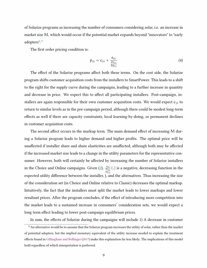
The Vrst order pricing condition is:

pjt = cjt +sjt∂sjt∂pjt

(4)

The eUect of the Solarize programs aUect both these terms. On the cost side, the Solarize

program shifts customer acquisition costs from the installers to SmartPower. This leads to a shift

to the right for the supply curve during the campaigns, leading to a further increase in quantity

and decrease in price. We expect this to aUect all participating installers. Post-campaign, in-

stallers are again responsible for their own customer acquisition costs. We would expect cjt to

return to similar levels as in the pre-campaign period, although there could be modest long-term

eUects as well if there are capacity constraints, local learning-by-doing, or permanent declines

in customer acquisition costs.

The second aUect occurs in the markup term. The main demand eUect of increasingM dur-

ing a Solarize program leads to higher demand and higher proVts. The optimal price will be

unaUected if installer share and share elasticities are unaUected, although both may be aUected

if the increased market size leads to a change in the utility parameters for the representative con-

sumer. However, both will certainly be aUected by increasing the number of Solarize installers

in the Choice and Online campaigns. Given (2), sjt∂sjt∂pjt

(.) is a negative, decreasing function in the

expected utility diUerence between the installer, j, and the alternatives. Thus increasing the size

of the consideration set (in Choice and Online relative to Classic) decreases the optimal markup.

Intuitively, the fact that the installers must split the market leads to lower markups and lower

resultant prices. After the program concludes, if the eUect of introducing more competition into

the market leads to a sustained increase in consumers’ consideration sets, we would expect a

long term eUect leading to lower post-campaign equilibrium prices.

In sum, the eUects of Solarize during the campaigns will include 1) A decrease in customer

11An alternative would be to assume that the Solarize program increases the utility of solar, rather than the market

of potential adopters, but the implied monetary equivalent of the utility increase needed to explain the treatment

eUects found in Gillingham and Bollinger (2017) make this explanation far less likely. The implications of this model

hold regardless of which interpretation is preferred.

9

acquisition costs; 2) An increase in market sizeM during the campaign (and possible a change

in the preferences of the representative consumer); and 3) an increase in consideration set sizes

from Choice and Online, which leads to lower optimal markups during and post campaign for

the Choice and Online towns, relative to the Classic towns.

After the campaigns conclude, we might expect a change in marginal cost for focal installers

through capacity constraints, local learning-by-doing, or permanent declines in customer acqui-

sition costs. If this were the case, there would be a long-term price eUect in the post-period for

all campaigns. There is no reason to expect a diUerent cost impact for Choice and Online relative

to Classic.

It could also be the case that any long-term eUects would be related to the markup term.

The increase in consideration set sizes from Choice and Online leads to lower optimal markups

during and post campaign for the Choice and Online towns, relative to the Classic towns. It

would also lead to price eUects for all installers in the market, whereas if the eUect of adding

competition worked through long-term eUects on marginal costs, we would expect the focal

installers to have larger long-term price eUects.

If the optimal makeup does change due to the increased competition, in addition to the price

eUect, shares for installers will be smaller, and there will be more competition in the marketplace

and less market concentration, all testable implications. The lower prices will also lead to higher

post-campaign demand relative to the single installer campaigns, in which prices may return to

pre-campaign levels or even increase if capacity constraints lead to temporary increase in the

marginal cost cjt. One reason for such long lasting eUects on consideration sets include word-

of-mouth (WOM) in which consumers refer their installers to others’, or through a decrease in

market level marginal costs for installers who have previously operated within that market.

We illustrate these eUects in Figures 1 and 2, using simple linear demand and supply curves

for illustration purposes only. In Figure 1(a), we show the shifts in demand and supply from a

Classic program which results in a dramatic increase in equilibrium quantity and a price eUect,

as determined by the relative changes to the supply and demand curves. In the post period, the

installer once again is responsible for its own customer acquisition and so we draw the supply

curve as the same as in the pre-campaign level, as shown in Figure 1(b) which would be the case

if there was no change on the optimal markups (and no large eUect on marginal costs in the short

10

term for the focal installer, leading to lower short term competition). Of course there might be

some long-term supply shift, but it is an empirical question.

In Figure 2, we show the expected eUects of a Choice or Online campaign. All of the focal

installers experience the reduction in their acquisition costs. For simplicity, we assume the same

eUect of the campaign on total demand in Classic. But because of the increased size of consumers’

consideration sets, the installers will price lower relative to the Classic program, and they will

split the total demand during the campaign. The resultant equilibrium price is lower than in

Classic, and the quantity is higher as well due to the greater shift in the aggregate supply curve.

In the post period (Figure 2(b)), increased consideration set sizes will lead to lower equilibrium

post-solarize prices as well, and higher quantities relative to Classic because of a permanent shift

to the right of the supply curve.

Our model leads to clear testable implications: if allowing multiple installers to operate

within the Solarize program does indeed increase consumer consideration sets sizes by increas-

ing the number of considered installers, then we should see long lasting eUects of these short-

term campaigns. The post campaign eUects include an increase in the number of active installers,

a decrease in HHI, a decrease in price for all installers, and an increase in demand (all relative to

that found in the Classic Solarize program).

4 Data

The primary data source for this study is the database of all solar PV installations that received

a rebate from the CGB, 2004-2016. When a contract is signed to perform an installation in CT,

the installer submits all of the details about the installation to CGB in order for the rebate to be

processed. As the rebate has been substantial over the the past decade, we are conVdent that

nearly all, if not all, solar PV installations in CT are included in the database.12

For each installation the dataset contains the address of the installation, the date the contract

was approved by CGB, the date the installation was completed, the size of the installation, the

pre-incentive price, the incentive paid, whether the installation is third party-owned (e.g. so-

12The only exception would be in three small municipal utility regions: Wallingford, Norwich, and Bozrah. We

expect that there are few installations in these areas.

11

lar lease or power-purchase agreement), and additional system characteristics. For Online, we

also have the bid data for the 327 customer requests (call for bids) submitted by potential solar

customers through the EnergySage platform.13

The secondary data source for this study is the U.S. Census Bureau’s 2009-2013 American

Community Survey, which includes demographic data at the municipality level. Further, we

include voter registration data at the municipality level from the CT Secretary of State (SOTS).

These data include the number of active and inactive registered voters in each political party, as

well as total voter registration (SOTS 2015). We match the installation data with the demographic

and voter registration data at the census tract level. Finally, campaign participants are sent an

online survey after the conclusion of the campaign.14

We standardize the time period that we include in our analysis relative to the Solarize cam-

paign starting dates. For each campaign, we consider 24 month pre Solarize, the Vve month

Solarize campaign, and 12 month post campaign period. This approach allows us to compare

the treatment eUects across campaigns relative to the Solarize interventions, and allows us to

test for persistent market outcomes (see also Allcott and Rogers 2014). For round 3 we consider

the full set of untreated clean energy communities as control towns.15 For round 5, we exclude

the 10 largest towns, resulting in 45 control municipalities. This adjustment ensures that we are

indeed comparing similar towns as treatment towns in later rounds have been slightly smaller.

As robustness, we verify that the choice of control towns does not impact our main results.

In order to assess the trends in prices and quantities, Figure 3 shows the cumulative uptake of

installations as well as the mean prices (third-party owned installations excluded) for the entire

sample period in the three groups. Both treatment groups as well as the control group have

parallel pre-treatment trends.16 The appendix (Figure A.1) also presents histograms of the main

dependent variables. Town demographics for treatment and control groups one year prior to the

13Note that in Online the conversion rates have been lower than in other type of Solarize campaigns, about 20%

(67 contracts signed).14Due to the community engagement, response rates for solar adopters were unusually high (close to 40%). In

addition we surveyed non-adopters, as well as performed personal interviews with the group of solar ambassadors.15CT Clean Energy Communities make a "Municipal Pledge" to save energy and voluntarily purchase renewable

energy.16In line with the visual inspection of the pre-treatment trends, we test for equal means of the Vrst-diUerences

one year prior to Solarize and do not Vnd evidence for statistic diUerences between the groups.

12

Solarize intervention are presented in Tables A.2 and A.3. The tables show that the distribution

of key demographic variables across treatment and control towns is indeed very similar.17

5 Descriptive Evidence

5.1 The eUect on the level of competition

Using the exogenous change in the number of selected Solarize installers leads to important

experimental variation in the amount of competition in the market. Table 1 provides evidence

on the average market concentration and the number of active installers per municipality in

Vve-month intervals relative to the Solarize campaign timing. The median number of bids in

Online is 3.01 with standard deviation 1.36, and so the number of active Solarize installers is

quite similar for both Choice and Online.

Focusing Vrst on the period ‘during Solarize’, we Vnd that both Choice and Online lead to a

signiVcant increase in active installers per town relative to the Classic campaigns. This is in line

with the experimental design, allowing for a larger number of selected installers. As expected,

we also see that the number of active installers remains higher in the Vve-month period after the

policy intervention.

In order to Vrst assess the diUerential eUect of adding more competition on market concen-

tration, we look at the means of the normalized HerVndahl-Hirschman Index (HHI) in the same

time periods. While Choice and Classic municipalities show very similar market concentration

in the pre-period (panel a), the single focal installer in Classic leads to a dramatic increase in

concentration (an HHI of 0.63 compared with 0.19 in Choice towns). As predicted, we Vnd that

Choice towns have more active installers in the post period relative to Classic towns, which also

leads to lower market concentration.

R5 reveals slightly diUerent numbers. As the overall market has matured importantly in

2014-15, we see a larger number of active installers to begin with. Yet, similar to the case of

Choice, Online leads to a signiVcantly larger increase in the number of active installers during

the campaign compared to Classic. This results in lower market concentration. On the other

17Statistical diUerences for key demographics can be only found for household income in Table A.2, and for the

share of homeowners and number of registered republican voters in Table A.3.

13

hand, the market concentration indices in the post-period are very similar for Online and Classic.

This could be a Woor eUect, which results from how low the concentration is in the post-period

for both campaign types. Online still leads to a signiVcantly larger increase in the number of

active installers post-campaign relative to Classic.

5.2 The eUect on shares and prices

In terms of market shares, the shares of focal installers increased in R3 Classic by 28% and in

Choice by 81%, relative to their pre-Solarize shares. The greater competition in Choice clearly

led to a larger post-campaign increase in focal installer market share. SolarCity shares increased

similar for both campaign types, by 23% and 25%, respectively.

In R5, we see a similar eUect from introducing more competition during the program. In

Classic, the post campaign share for the focal installers increased 52%, relative to 175% for On-

line installers. Unlike in R3, SolarCity shares decreased as a result of both, by 31% and 42%,

respectively. In contrast, SolarCity shares increased for the control group in R5. Thus, the in-

crease in focal installer share during R5 for both Classic and Online came at the expense of the

now established market leader, SolarCity.

Descriptive evidence of the heterogeneous impact of distinct Solarize interventions on system

prices are given by Figure 4 which shows the mean price of solar installations by the type of

system Vnancing. Solar installations are either purchased, Vnanced though a loan, or installed

with third-party ownership either through a lease or power purchasing agreements (PPA). Since

the type of Vnancing can have an important impact on the cost per Watt of a solar installation,

Figure 4 compares average prices by type of Vnancing. The Vgure shows the average price as

well as standard deviation for R3 (Choice vs. Classic vs. Control) and R5 (Online vs. Classic vs.

Control) in Vve-month intervals relative to the Solarize campaign. Panel (a) reveals that both

Classic and Choice led to an important drop in prices during the campaign for Lease, Loan, and

Purchase products. Moreover, purchase prices remain low in the post-campaign period. PPA

installations, on the other hand, show very little price movement. Panel (b) of the same Vgure

compares prices for R5 and tells a similar story. Overall we Vnd that the Solarize campaigns lead

to an important price decrease during the campaign, with a larger drop for Choice and Online

compared to Classic. These insights are in line with our theoretical predictions. The eUect for

14

post-campaign prices is not as clear when comparing unconditional means.

Figure 5 provides insights on the pricing of Solarize installers versus competitors in the

same towns; clearly, the focal installers in Solarize towns are more competitive to begin with.18

However, the price diUerences can be partially explained by the Vnancing composition of these

groups, as it is mainly focal installers that sell purchased and Vnanced installations, while some

competitors engage in the PPA market.19 Comparing diUerences within groups over time, an

increase in competition seems to be not only related to a larger drop during the campaign, but

a prolonged drop in the post-period. Finally, the price of non-focal installers in Solarize towns

reWect closely the price of solar installations in control towns.

Another explanation for the post-campaign price diUerences is that is that the type of Solar-

ize campaign aUects the composition of product Vnancing or size of installations. To assess this,

Figures A.3 and A.4 present the mean Vnancing shares as well as size distributions for the dif-

ferent campaigns. While Figures A.3 shows clearly that Solarize lead to more purchase-Vnanced

installations during the campaign, post-campaign Vnancing shares are similar across all cam-

paign types and the control group. More importantly, diUerent type of Solarize campaigns did

not lead to diUerent Vnancing shares.

Fig A.4 shows that the distribution of system sizes in the post period in R3 was not aUected

by Solarize, although system sizes were slightly larger during the campaigns. In R5, the sizes

are slightly larger in the pre period. In our regression framework, we condition on the type of

system Vnancing, system size, and system mounting when estimating the main price eUect.

6 Empirical SpeciVcation

To quantify the equilibrium impact of increasing competition on equilibrium prices, we regress

the installation-level cost of solar PV on treatment dummies, a rich set of individual controls as

well as time and municipality Vxed-eUects. The regression equation is:

Priceimt = α+ δsTmt + γsPmt + βX + θm +ψt + εimt (5)

18As installers actively bid for towns this insight is in line with the Solarize design.19 A.2 in the appendix shows the shares by type of Vnancing.

15

where Priceimt represents the price ($ per kilowatt) of solar installation i, in municipalitym, at

time period t. Tmt is a treatment dummy variable and Pmt is a post-treatment dummy.

The eUects of the treatments during the campaigns and afterward, δs and γs, depend on the

type of Solarize campaign, indicated with the s subscript. The regression includes municipality

and month Vxed-eUects (FE) to account for both time-invariant diUerences across municipalities

and aggregate shocks to the CT solar market. The control vector X includes observable char-

acteristics of the solar installations such as system size, type of system mounting and system

Vnancing.20 All standard errors are clustered at municipality level, in order to account for error

correlation within the same municipality over time. We estimate equation (5) for each round

separately. We are interested in comparing the treatment eUects and post-treatment eUects for

Choice and Classic in the R3 regression as well as Online and Classic in R5.

To better study the adjustment dynamics, we estimate a variation of (5). Using an event

study design (similar to Gallagher 2014), we introduce a full set of time dummies that is allowed

to vary by group (Classic, Choice or Online, Control) and estimate the price impact relative to

the Solarize intervention.21All results are relative to the two-month period pre-intervention.22.

Besides, these alteration, the regression model contains all additional variables that have been

used in speciVcation (5).

6.1 Quantity regression

An additional outcome of interest are the equilibrium quantities sold in each market. For this

purpose, we aggregate our data at the monthly level and estimate a classical diUerence-in-

diUerence (DiD) estimator to test for the impact of competition on quantities sold. The quantity

20For robustness, we experiment with diUerent time Vxed-eUects (quarterly, annual combined with monthly dum-

mies). The main Vndings are robust to the choice of FE.21As there are certain month with zero installations, we include one separate dummy for each two-month interval.

Moreover, as there have been few installations in the Vrst months of our sample, we group these early installations

(24 month to 13 month prior to the campaigns) into a single dummy.22This category is omitted from the regression.

16

model is estimated both by ordinary least squares using a diUerence-in-diUerence mode23:

Instmt = α+ δsTmt + γsPmt + βX + θm +ψt + εmt (6)

where Instmt is the total number of new solar installations in municipality m, at time t. As in (5),

the model includes both municipality and month Vxed-eUects (FE). Our main interest again lies

in the comparison of treatment (δs) and post-treatment (γs) coeXcients. To better understand

the dynamics, we follow the same event study design approach as outlined above. Moreover, as

the main dependent variable in (6) is count data, we estimate the model both by ordinary least

squares and by Vtting a negative binomial count data regression.

7 Results

7.1 Impact of competition on equilibrium prices and quantities

7.1.1 Prices

The main regression results from equation (5) for both R3 and R5 are displayed in Table 2. Col-

umn 1 estimates the model without control variables, while column 2 includes controls for sys-

tem Vnancing, system size, and system mounting. The reference category are purchase-Vnanced

installations.

We Vnd that controlling for individual system covariates is important to obtain precise (un-

biased) treatment eUects, which highlights the importance of using detailed micro-data in the

analysis. Focusing on the R3 results in column 2 with size, mounting and Vnancing controls, we

show that while Solarize Classic leads to a price decrease of about 29 cents per watt installed, the

price impact of Choice is considerably larger at 49 cents perWatt. While the post-campaign dum-

mies are not signiVcant relative to the control group, an F-test establishes that the post-campaign

prices after Choice are signiVcantly lower than after Classic (p = .027). One explanation in the

suggestive increase in prices relative to the control is short term capacity constraints as result

of the campaign due to frictions in labor supply, which is consistent with anecdotal evidence we

have collected from speaking with installers.

23We will show robustness to the use of a negative binomial count model.

17

Columns 3 and 4 display the main results for R5, comparing Online and Classic. Without the

controls, we Vnd similar results as in R3, but controlling for system size, mounting and Vnancing

shows that the interventions in R5 did not have a price impact during the campaign. Again,

whether there is an equilibrium price eUect is an empirical question and is determined by the

relative shifts of the supply and demand curves. This indicates that the demand curve shifted

more in R5, or the supply curve shifted less. Similar to Choice in R3, we Vnd that there is a

signiVcant eUect in the post campaign period with Online leading to lower prices than Classic

(p = 0.04).

As it has been pointed out, the CT solar market has evolved importantly between R3 and

R5 and new types of Vnancing were beginning to increase their market shares. As the overall

market is more competitive, we see smaller price drops due to Solarize. It is thus not surprising

that the additional competition led to only an 18 cents per kW drop in Online relative to Classic

in the post-solarize period, in contrast to the 30 cent diUerence between Choice and Classic in

R3.

Although our outcomes of interest, the price of solar installations, are at the individual level,

since Solarize campaigns are randomized at municipality level we use clustered standard errors in

order to not overstate the precision of our estimates. That said, our results still rely on asymptotic

arguments ti justify the normality assumption. We can address this concern using randomization

inference (Fisher 1935, Rosenbaum 2002). Randomization inference (RI) has found increasing

attention in studies dealing with small sample size (see for example Bloom, Eifert, Mahajan,

McKenzie, and Roberts 2013, Cohen and Dupas 2010). The main advantage of RI is that it does

not need any asymptotic arguments or distributional assumptions.

In order to test for the causal impact of the Solarize treatment, we group our data in diUerent

sub-samples to perform each pairwise comparison for Classic, Choice (or Online), and the control

group, for example keeping only Solarize Classic and Control municipalities for Round 3. We

then randomly assign treatment status at the municipality level and re-estimate our original

regression model (5). The two coeXcients of interest are the main treatment eUects and the

18

eUects in the post-intervention period.24 In Table 3, we report the estimated coeXcients using

each subsample with the clustered standard errors, as well as the results of the randomization

inference. These Vndings conVrm our main results, showing that Choice and Online towns led to

signiVcant lower prices both during and post-campaign compared to the single installer case. As

an alternative, we also address the small sample sizes using the wild cluster bootstrap, discussed

more in the robustness checks.

We perform a series of additional robustness checks concerning our main results. In particu-

lar, we limit our sample to cash-purchased installations only.25 We provide additional robustness

checks for the impact of focal installers as well as the main economic speciVcation. Finally, we

experiment regarding pre- and post-periods and concerning the group of included control mu-

nicipalities. Our main results are robust to these robustness checks. We further conVrm the

signiVcance of our Vndings using the wild cluster bootstrap which also does not rely on asymp-

totic arguments.

7.1.2 Quantities

In order to better understand the equilibrium price response to increased competition, we need

to also assess what happens to quantities. To that purpose we estimate model (6), aggregating the

data at municipality-month level. Columns 1 and 2 of Table 4 shows the main treatment eUects

for Classic and Choice in R3. While column 1 does not control for any additional covariates, col-

umn 2 includes the share of Vnancing to control for compositional eUects. In both speciVcations,

we Vnd that Choice leads to 1.3 to 1.5 additional monthly installations during the campaign (ap-

proximately 7 installations for a Vve-month campaign), which represents an increase of roughly

25% when evaluated at the mean number of monthly installations during Classic.26

If we assume that the shift in the demand curves are comparable across campaigns in R3,

24We simulate 1000 data draws and perform a left-tail test, comparing the simulated coeXcients to our original

estimates. The p-value is given by the number of simulations that lead to smaller treatment eUects as the original

sample divided by the number of simulations.25The cost information for leasing products as well as loan-Vnanced installations might contain measurement

errors as this information cannot be perfectly observed by the CT Green Bank.26The total number of installations in Choice are displayed in Table A.1. On average, there have been 6.86 new

installations per month of Solarize.

19

then the price and quantity changes in Choice vs. Classic in R3 give us two points on the de-

mand curve (exploiting the experimental shift in the supply curve). The implied price elasticities

are -4.6 during the campaign and -3.6 after the campaign. These are higher than that found by

Gillingham and Tsvetanov (2015), implying that the campaigns may have indeed expanded the

market to include more than just the less-elastic "innovators" in the market. Since all elasticities

are estimates for the marginal consumers, this is clear evidence that the marginal consumer has

changed as a result of the campaign. This also supports our proposed interpretation of the quan-

tity treatment eUects from Solarize found in Gillingham and Bollinger (2017) as an expansion of

the market.

These points are subject to the caveat that the quantity eUects are imprecisely estimated.

Even though the points estimates are large, we cannot reject the null hypothesis of equality of

coeXcients. We also Vnd evidence that Classic leads to some harvesting (negative and signiVcant

coeXcient in both speciVcations in the post period), while this is not true for Choice. We hence

Vnd that increasing competition in the Choice campaigns leads to more product sales during the

campaigns and more importantly there is limited evidence for harvesting in the post-campaign

period. It could be that this is also reWecting the impact of the long-term price eUect we found

for Choice relative to Classic in the post periods.

Columns 3 and 4 of Table 4 present the estimation results for Classic and Online. While Clas-

sic led to about 5.5 additional installations during each campaign month , Online was responsible

for only 3 additional installations. Note that the overall market expansion from R3 to R5 has led

to more solar uptake in the state, so that the quantity eUects for Classic are comparable across

rounds. Given the very diUerent nature of the online campaign, the demand curve shifts clearly

are diUerent for Online and Classic, making the elasticity calculation impossible. One obvious

question is why did Online lead to little additional sales if prices were lower? We explore this

question further using the survey data below.

20

7.2 EUect persistence

Another way to look at the main cost dynamics without making any assumptions about the

precise campaign timing27 is to use the time dummy approach as explained in Section 6. Figure 6

plots the individual estimates for two-month intervals for the three groups in R3, Classic, Choice,

and Control, relative to the Solarize timing. The Vgure shows both point estimates and the 95 %

conVdence bands. The two month period prior to the Solarize intervention are omitted from the

regression. Panel (a) shows clearly that while prices in Control towns have been not aUected by

the Solarize intervention, both Classic and Choice led to a drop at the beginning of the campaign

period. However, while prices in Classic stayed similar relative the baseline, Choice stayed at a

lower level for the entire year post-period. Panel (b) shows the same dynamic for Classic versus

Online in R5. round 5. Although prices co-moved for most of the periods (prices in Online were

slightly lower during the campaigns), Online prices dropped even further around the Vve-month

post-campaign point, possibly due to the free entry of competitors.

In line with the price regression, we estimate a variation of model (6), including separate

two-month time dummies for each of the campaigns to better analyze the dynamics (i.e. estimat-

ing time x campaign type interactions). Figure 7 plots the point estimates and 95% conVdence

intervals for the impact of Solarize on equilibrium quantities. Panel (a) shows clearly that in

the pre-intervention period, Classic and Choice towns had very similar uptake rates, and only

three months into the campaign do people in the Solarize Choice municipalities start installing

more solar panels. This larger eUect is persistent in the post-period, and only one year after

the campaign do the number of new installations converge. Panel (b) of the same Vgure shows

the quantity dynamics for R5. In line with our main regression, we Vnd that Online leads to

less additional uptake. Interestingly, the main diUerence between the campaigns occurs in the

last months of the campaign, indicating that the single installer in Classic did a better job in

converting sales leads.28 The post-campaign period was unaUected (in terms of quantity) by the

27Some installations might happen after the oXcial end of the Solarize campaign, but might still receive the

price-beneVts of Solarize.28The particular rough winter 2014/15 led to cancellation of site visits and to postponement of scheduled events.

This partially explains the lower uptake in R5 compared to R3. Moreover, in Classic, the single installer had a greater

ability to make a sales push in the last months of the campaign and to recover sign-ups. The setup of Online did not

allow for this direct sales interaction.

21

campaigns. Finding no evidence for a signiVcant quantity response in the pre-treatment time

dummies provides a Vrst robustness-check ruling out consumer anticipation of the campaigns.

7.3 EUects by installer

Our proposed mechanism behind the diUerences in prices between Classic programs and those

with more competition is that when there are more program installers, consideration sets are

increased (permanently). This leads to a smaller diUerence in consumer utility in the post-

campaign period between the focal installer(s) and the non-foal installers, because the focal

installers in Choice and Online have to split the market, which leads to smaller optimal markups

(relative to having a single focal installer). It is not clear whether the observed price decrease

has been driven by focal installers alone or if the Solarize campaigns have led to an overall

price changes in campaign municipalities. Table 5 shows the additional price eUects for focal in-

staller(s), interacting the treatment dummies in main speciVcation (5) with an indicator variable

for the focal (selected) Solarize installer.29

As before, columns 1 and 2 show the main eUects for R3; although no individual point esti-

mates are signiVcant, the size and sign are in line with the main results. The large standard errors

can be explained by the small number of focal-installer sales in the pre-and post-Solarize periods

(see Table A.1) as well as heterogeneity across markets.30 In R3, the results are suggestive that

prices decline more for the focal installers during the campaigns, which is what we would expect

given the reduction in customer acquisition costs. The results also suggest that prices decline

more in Choice relative to Classic both during the campaign an in the post period. However in

contrast to the eUects during the campaign, after the campaigns there is no discernible diUer-

ence in the prices for focal and non-focal installers. This is more consistent with our proposed

explanation of increased competition in the post-Solarize period than persistent declines in costs

for the focal installers.

For R5, prices are lower in the post period for the non-focal installers but are actually higher

for the focal installers. Part of this could be explained by more binding capacity constraints, but

29The number of active focal installer in Choice and Online can be found in Table A.1.30Running the main regression only on the sub-sample of installations done by focal installers leads to a highly

singular covariance matrix.

22

we also see that the price increase by focal installers in the post-campaign period is smaller for

Online than for Classic. The most likely explanation is that in R5, the utility of the focal installers

increase relative to the other adoption alternatives, leading to an increase in market power and

optimal markup. This increase is smaller in Online because all the installers that participated in

the program beneVted in this way.

A persistent cost decline for focal installers would have implied lower prices for the focal

installers after all the campaigns. We see no diUerence in R3, and higher prices for focal installers

after R5. The larger price declines for campaigns with more competition (Choice and Online) also

indicate that the likely explanation for the long term price eUects is from changes in markups,

not costs. To explore why prices actually increase after R5 for the focal installers, it is helpful

to examine the consumers’ likely alternatives, not purchasing solar or purchasing from the main

non-focal installer, SolarCity.

In many locations in R3, the Solarize campaigns coincided with the entry of SolarCity, the

largest provider of solar energy services in the US and started targeting the residential solar

market in Connecticut in mid 2012. SolarCity is the main provider of PPA’s, oUering solar instal-

lations at zero down payment. If SolarCity focused on speciVc Solarize municipalities, it would

aUect the post-campaign market structure.

SolarCity was active in 11 of 16 Solarize markets prior to the start of R3, and all but one

at the start of R5. In Figure 8, we compare the mean SolarCity market shares in the pre- and

post-campaign periods for diUerent campaigns.31 In both campaign types and the control group,

the share of SolarCity increases from the pre-campaign to post-campaign period. In R5, this is

also true for the control group, but the opposite is true for the campaigns. This indicates that

the Solarize campaigns in R5 lowered the market share of SolarCity, again providing evidence

for a persistent eUect on the focal installers’ market power which is reWected in their prices.32

In accordance with our random utility model, the campaigns increased the market power for

the focal installers relative to the non-focal alternatives, leading to the increase in optimal price

post-campaign, a smaller increase for Online in which consumers still have the choice between

multiple participating installers.

31Table A.1 shows the market shares of SolarCity in R3 and R5 by town.32We test for equality of market shares using an ANOVA analysis and can reject the null hypothesis of equal

market shares across treatments in round 3 and 5.

23

7.3.1 Survey data

In order to help asses the impact of the Solarize programs, we surveyed solar PV adopters, as

well as non-adopters, after each Solarize round.33 The e-mail addresses came from Solarize event

sign-up sheets and installer contract lists. Approximately 6 percent of the signed contracts did

not have an e-mail address. All others we contacted approximately one month after the end of

the round, with a follow-up to non-respondents one month later. The overall response rates for

adopters was 42.2 percent (496/1,175). This high response rate is a testament to the enthusiasm

of the adopters in solar and the Solarize program.

The survey includes several questions concerning customer satisfaction with the solar instal-

lation (quality measure) as well as concerning the Online platform. First, we Vnd that on average

around 80-90% of adopters report ‘being very satisVed or satisVed with their installation’, inde-

pendent of the type of campaign. The very high satisfaction consumers had with their installer

during the program, coupled with the peer eUects shown in Bollinger and Gillingham (2012)

more generally for solar, and in Gillingham and Bollinger (2017) for the Solarize CT programs

provides an explanation for why consumer consideration sets would see a long-lasting increase

as a result of the 20-week Solarize Choice and Online programs, leading to the long-term price

declines. If consumers share their positive experiences with others in the community, all focal

installers would be expected to maintain a market presence after the campaign, which is indeed

what we Vnd.

For the Online campaigns, we explicitly asked about the role of the platform in leading to

larger consideration sets (we did not ask in Choice although the inclusion of multiple focal in-

stallers throughout the campaigns at events, etc. ensures it.). We found that 88% of survey

participants said they ‘liked the option of having distinct installers to choose from’, providing

strong support for our proposed mechanism. The respondents also reported that the ‘website was

a useful source of information’ (76%) and that ‘installers responded timely’ to requests (84%).34

Helping to explain the small treatment eUect for quantities in Online compared to Classic, re-

spondents noted that although the website itself was ‘well organized and easy to use’, only about

33This survey was performed through the Qualtrics survey software and was sent to respondents via e-mail, with

2 iPads raYed oU as a reward for responding.34Percentage for individuals that either agree or strongly agree. N= 25, only Online campaign.

24

one third (36%) thought that ‘bids from diUerent installers were easy to compare’. This Vnding is

in line with anecdotal evidence that Online led to some confusion for potential adopters.

For each contract signed we observe the chosen installer and detailed product features (sys-

tem size, solar panel brand, inverter type and brand, total cost, type of Vnancing, estimated

annual production, as well as installation date). In total, there were 13 competitors participating

in the Online bidding with very heterogeneous bidding behavior.35 Overall customers appear to

be price sensitive. In the case of two or more competing oUers, 31% of customers decide for the

cheapest option (cost per Watt (pre-incentive) / system size), and close to 30% go with the second

cheapest option.36

7.3.2 Single installer vs. group pricing

One other diUerence between the Classic program and the Choice and Online programs is the

presence of group pricing. However, the addition of the group pricing cannot explain our results.

Gillingham and Bollinger (2017) analyze the impact of Solarize Classic campaigns that did not

have group pricing that were implemented during R5. They found that the campaigns without

group pricing (which had relatively modest price declines) were just as eUective as the Classic

campaigns. We use the data from these additional campaigns to perform randomization infer-

ence to further test for equality of the Classic campaigns with and without group price. The

results are in Table A.4. There are no signiVcant diUerences in campaign eUectiveness that result

from the presence of group pricing.

7.4 Robustness

We perform a series of additional robustness checks and Vnd similar results across all of them:

• Wild cluster bootstrap standard errors as developed in Cameron, Gelbach, and Miller

(2008). See Tables A.5 and A.6

35While one installer bid on all 67 projects, two installers on about 2/3 of all projects, and the rest presented bids

on 1/3 or a signiVcant lower share. Interestingly the Vrm with most quotes did only win 6% of all contracts. Other

large bidders have been more successful in their conversion rates.36Note that installations can be heterogeneous in many dimensions such as brand or eXciency. The small sample

makes it diXcult to pin down the precise factors inWuencing consumer decisions.

25

• Type of Vxed eUects (quarter and annual FE with month-of-year dummies)

• Log-transformed main dependent variable

• Robustness regarding the precise starting and end date of individual Solarize campaigns.37

• Sample selection: pre-and post Solarize time-periods included in the estimation. Limit the

sample to one year pre-intervention and to seven month post.

We also provide some robustness concerning sample selection in Tables A.7 and A.8. In

column 1 we estimate the main price regression (5) on purchase-Vnanced installations only.38

Column 2 limits the sample to rooftop installations with a system size smaller or equal 10 kilo-

watt. We additionally control for system Vnancing. The results for these sub-samples are very

much in line with the main results from Table 2. We Vnd a signiVcant and larger price decreases

for Choice and Online compared to Classic during the campaign. We also additional evidence in

line with the hypothesis that Choice and Online aUect prices in the post-campaign period.

For the quantity regressions, the main dependent variable, namely the number of new solar

installations, is heavily skewed (see Figure A.1. For robustness, we estimate model (6) using a

negative binomial model count data model. The results are presented in Tables A.9 and A.10 for

round 3 and round 5 respectively. The tables show the incidence-rate-ratios (IRR), which can

be interpreted as arrival rates. A coeXcient of one hence means translate into a zero treatment

eUect. For robustness, columns 1 and 2 present two distinct estimation methods.39 40 We Vnd

that the qualitative results are in line with our main estimates.

37As we do only observe the date at which the solar installation received approval by the CT GreenBank, but not

the precise installation date, some installations dated post-Solarize should still be counted to the campaigns. We use

data from installer to recover the average time gap between completion of installation and "approval date" of the

installation by the Green Bank. Our results are robust to the precise timing assumptions.38While our database contains price information on all type of Vnancing, the complexity of lease and loan prod-

ucts can lead to inaccuracies in reported costs, especially if the Vnancing products have been oUered through a

installer contract. Replicating our main results for purchase-Vnanced installations only is hence an important sign

of robustness.39The correct model selection in negative binomial models with high degree of FE is an active area of research.

See for example Guimarães (2008), http://www.stata.com/statalist/archive/2012-02/msg00399.html.40As additional robustness, we estimate model (2) with the subsample of rooftop installations only and experiment

with weighting according to market size (number of residential buildings) and the number of installations. The

qualitative results are robust.

26

8 Discussion

We Vnd that an increase in competition during Solarize (Choice & Online) leads to a price

drop about twice the size compared to the single installer case (Classic). Focusing on purchase-

Vnanced installations only, the price diUerence between Choice and Classic in round 3 is about

30 cents per Watt, while for Online and Classic (round 5) the diUerence is about 15 cents per

Watt. These diUerences cannot be explained by changes in product composition, i.e., changes in

the type of product Vnancing, size of installations, etc.

Focusing on quantities sold, we Vnd that Choice leads to 6.1 additional installations per

month of campaign, while Classic results on average in 4.5 new installations per month. While

we Vnd some evidence for harvesting in Classic towns, Choice did not lead to a signiVcant drop

in installation quantities in the post-campaign period. This eUect can be explained by two main

factors. First, several Solarize installers might be able to generate more attention throughout

the campaign, resulting in additional sales in the post-campaign period. Second, single Solarize

installers might be faced with capacity constraints and they might be unable to meet demand in

a timely manner in the post-period. The quantity response in Online are smaller than in Clas-

sic (3.2 installations versus 5.5 installations respectively), which can be explained by demand

side factors. In Online, we Vnd that a larger share of potential customers do not sign a purchase

contract. Choice overload and comparability of bids are potential reasons for the lower sales con-

version. The overall market in round 5 has expanded importantly with the entry of the largest

solar energy service provider in the United States, SolarCity, and the provision of new type of

product Vnancing.

In line with our model predictions, we Vnd that the higher degree of competition during

Solarize Choice and Online leads to long-term price declines in the post-campaign period. The

increased competition during the program leads to long term increases in the number of active

installers by 2-4 installers (an increase of 50- 100%) and a long term price decline of $0.18/W -

$.028/W. This equates to between $0.08/W and $0.09/W per extra installer, an elasticity of 0.11-

0.14. The fact that a temporary campaign can lead to these long term prices declines, increasing

consumer surplus, has large implications for government-business partnerships, speciVcally the

need to still foster competition within such initiatives.

Although the use of online platform did lead to a smaller quantity increase than Choice did

27

during and after the campaigns (relative their respective concurrent Classic campaigns), as con-

sumers become more familiar with using such platforms, and as the number of participating

installers increase, we would expect downward pressure on prices to continue. From a logisti-

cal standpoint, the EnergySage platform allows for a more open market environment and the

inclusion of all Vrms that want to participate (assuming they meet certain criteria), whereas

the Choice programs were logistically challenging and limited in the number of installers they

could include. Online platforms could easily see larger demand eUects if prices can be made

more comparable across options (something we were able to ensure in the Classic and Choice

program through the use of the RFP bid process).

The main limitation of this study is the sample size. Logistical and cost considerations are

the reason for the small number of towns in the experiment.41 However, these sample sizes are

not uncommon in the development economics literature, in which entire communities must be

randomly assigned as a unit, rather than randomization occurring at the household unit.42 Such

market-level randomization is necessary given the desired object of study, namely equilibrium

price and quantity eUects of competition. That said, our Vndings are very robust to alternative

speciVcations, and the very large lift that results from the campaigns leads us to estimate statis-

tically signiVcant results, even with the smaller sample size and after clustering standard errors

at the town level.

Despite the detailed information on individual campaigns (events, post-campaign surveys

with ambassadors and participants, installer surveys, etc.), with the small sample it is hard to

fully explain the mechanism for the equilibrium results and heterogeneity across the campaigns

with revealed preference data alone, since we have limited degrees of freedom. The Vnal esti-

mates include any eUects that result from coordination between the town, installers, Smartpower,

and in the case of Online, the EnergySage platform. The eUect of adding competitors may have

also aUected the eUectiveness of ambassadors43 and the communication strategy of installers

41The cost of the 28 towns in R3 and R5 alone exceeded $800,000.42The paper most related to ours is Busso and Galiani (2014), in which the authors test for the impact of increased

competition on market outcomes in the development context. The authors rely on random variation from the

implementation of a conditional cash transfer program in the Dominican Republic. They Vnd that six months after

the intervention, product prices in the treated areas had decreased by about 6%, while product quality and service

quality was not aUected by the entry of new competitors.43In another paper, Kraft-Todd, Bollinger, Gillingham, Lamp, and Rand (2017) analyze the impact that personality

28

with the town (e.g. a single focal installer might have been able to provide a clearer message

than several competing Vrms). However, the combination of the large-scale Veld experiment

with the extensive survey data do allow us to further examine the mechanisms of the interven-

tions. The very high satisfaction of consumers with their installers and the importance of WOM

lead us to believe that market power through WOM eUects leading to larger consideration set

sizes in the post-campaign periods lead to the long term eUects.

9 Conclusion

This paper provides new evidence for a classic question concerning the equilibrium price and

quantity impacts of competition. Taking advantage of experimental variation in the number of

competitors allowed to operate within a large-scale marketing campaign (Solarize Connecticut),

our Vndings conVrm the classic result that an increase in competition lowers prices, and hence

increases consumer surplus. We also Vnd limited evidence that increased competition leads to

larger product adoption that is persistent in the post-treatment period. These Vndings have im-

portant policy implications; government has increasingly worked through business partnerships

to achieve policy goals in domains such as energy, health, education, and crime prevention. Al-

though such partnerships may help achieve the end objectives, this paper highlights the risks

when such partnerships are exclusive because competition remains critical in reducing costs in

the long run.

References

Aghion, P., S. Bechtold, L. Cassar, andH. Herz (2014): “The causal eUects of competition on innovation:

Experimental evidence,” Discussion paper, National Bureau of Economic Research.

Allcott, H., and S. Mullainathan (2010): “Behavior and energy policy,” Science, 327(5970), 1204–1205.

Allcott, H., and T. Rogers (2014): “The short-run and long-run eUects of behavioral interventions:

Experimental evidence from energy conservation,” The American Economic Review, 104(10), 3003–

3037.

traits of the ambassadors have on the campaign success.

29

Angrist, J. D., and J.-S. Pischke (2010): “The Credibility Revolution in Empirical Economics: How Better

Research Design is Taking the Con Out of Econometrics,” Journal of Economics Perspectives, 24(2),

3–30.

Ashraf, N., O. Bandiera, and B. K. Jack (2015): “No Margin, No Mission? A Field Experiment on

Incentives for Public Service Delivery,” Journal of Public Economics, forthcoming.

Bain, J. S. (1951): “Relation of proVt rate to industry concentration: American manufacturing, 1936–1940,”

The Quarterly Journal of Economics, 65(3), 293–324.

BenYishay, A., and A. M. Mobarak (2014): “Social Learning and Communication,” Yale University Work-

ing Paper.

Berger, A. N., and T. H. Hannan (1989): “The Price-Concentration Relationship in Banking,” The Review

of Economics and Statistics, 71(2), 291–299.

Berry, S. T. (1992): “Estimation of a Model of Entry in the Airline Industry,” Econometrica: Journal of the

Econometric Society, pp. 889–917.

Bertrand, J. (1883): “Review of Cournot’s Rechercher sur la theorie mathematique de la richesse,” Journal

des Savants, pp. 499–508.

Bloom, N., B. Eifert, A. Mahajan, D. McKenzie, and J. Roberts (2013): “Does management matter?

Evidence from India,” The Quarterly Journal of Economics, 128(1), 1–51.

Bollinger, B., and K. Gillingham (2012): “Peer EUects in the DiUusion of Solar Photovoltaic Panels,”

Marketing Science, 31(6), 900–912.

(2016): “Learning-by-Doing in Solar Photovoltaic Installations,” Yale University Working Paper.

Borenstein, S., and N. L. Rose (1994): “Competition and price dispersion in the US airline industry,”

Journal of Political Economy, 102(4), 653–683.

Bresnahan, T. F. (1989): “Empirical studies of industries with market power,” Handbook of industrial

organization 2, pp. 1011–1057.

Bresnahan, T. F., and P. C. Reiss (1990): “Entry in monopoly market,” The Review of Economic Studies,

57(4), 531–553.

(1991): “Entry and competition in concentrated markets,” Journal of Political Economy, 99(5),

977–1009.

Busso, M., and S. Galiani (2014): “The causal eUect of competition on prices and quality: evidence from

a Veld experiment,” Discussion paper, National Bureau of Economic Research.

30

Cameron, A. C., J. B. Gelbach, and D. L. Miller (2008): “Bootstrap-based improvements for inference

with clustered errors,” The Review of Economics and Statistics, 90(3), 414–427.

Cohen, J., and P. Dupas (2010): “Free distribution or cost-sharing? Evidence from a randomized malaria

prevention experiment,” The Quarterly Journal of Economics, pp. 1–45.

Cotterill, R. W. (1986): “Market Power in the Retail Food Industry: Evidence from Vermont,” The Review

of Economics and Statistics, 68(3), 379–386.

Dai, M., Q. Liu, and K. Serfes (2014): “Is the eUect of competition on price dispersion nonmonotonic?

Evidence from the US airline industry,” The Review of Economics and Statistics, 96(1), 161–170.

Domowitz, I., R. G. Hubbard, and B. C. Petersen. (1986): “Business cycles and the relationship between

concentration and price-cost margins,” The RAND Journal of Economics, pp. 1–17.

Duflo, E., and E. Saez (2003): “The Role of Information and Social Interactions in Retirement Plan Deci-

sions: Evidence From a Randomized Experiment,” Quarterly Journal of Economics, 118(3), 815–842.

Dufwenberg, M., and U. Gneezy (2000): “Price competition and market concentration: an experimental

study,” international Journal of industrial Organization, 18(1), 7–22.

Einav, L., and J. Levin (2010): “Empirical industrial organization: A progress report,” The Journal of

Economic Perspectives, 24(2), 145–162.

Ellison, G., and S. F. Ellison (2009): “Search, obfuscation, and price elasticities on the internet,” Econo-

metrica, 77(2), 427–452.

Evans, W. N., and I. N. Kessides (1993): “Localized Market Power in the U.S. Airline Industry,” The Review

of Economics and Statistics, 75(1), 66–75.

Favara, G., and J. Imbs (2015): “Credit Supply and the Price of Housing,” American Economic Review,

105(3), 958–992.

Fisher, Ronald, A. (1935): “The design of experiments,” London: Oliver and Boyd.

Gallagher, J. (2014): “Learning about an infrequent event: evidence from Wood insurance take-up in the

United States,” American Economic Journal: Applied Economics, 6(3), 206–233.

Geostellar (2013): “The Addressable Solar Market in Connecticut,” Report for CEFIA.

Gerardi, K. S., and A. H. Shapiro (2009): “Does competition reduce price dispersion? New evidence

from the airline industry,” Journal of Political Economy, 117(1), 1–37.

Geroski, P. A. (1995): “What do we know about entry?,” International Journal of Industrial Organization,

13(4), 421–440.

31

Gillingham, K., and B. Bollinger (2017): “Social Learning and Solar Photovoltaic Adoption: Evidence

from a Field Experiment,” Unpublished mimeo.

Gillingham, K., H. Deng, R. Wiser, N. Darghouth, G. Barbose, G. Nemet, V. Rai, and C. Dong (2016):

“Deconstructing Solar Photovoltaic Pricing: The Role of Market Structure, Technology, and Policy,”

Energy Journal, 37(3), 231–250.

Goolsbee, A., and C. Syverson (2008): “How do incumbents respond to the threat of entry? Evidence

from the major airlines,” The Quarterly journal of economics, 123(4), 1611–1633.

Graham, D. R., D. P. Kaplan, and D. S. Sibley. (1983): “EXciency and competition in the airline industry,”

The Bell Journal of Economics, pp. 118–138.

Graziano, M., and K. Gillingham (2015): “Spatial Patterns of Solar Photovoltaic System Adoption: The

InWuence of Neighbors and the Built Environment,” Journal of Economic Geography, forthcoming.

Harrison, G. W., and J. A. List (2004): “Field experiments,” Journal of Economic literature, 42(4), 1009–

1055.

Holmes, T. J. (2011): “The DiUusion of Wal-Mart and Economies of Density,” Econometrica, 79(1), 253–302.

Jacobsen, G., M. Kotchen, and G. Clendenning (2013): “Community-based Incentives for Environmen-

tal Protection: The Case of Green Electricity,” Journal of Regulatory Economics, 44, 30–52.

Jia, P. (2008): “What happens when Wal-Mart comes to town: An empirical analysis of the discount

retailing industry,” Econometrica, 76(6), 1263–1316.

Kraft-Todd, G. T., B. Bollinger, K. Gillingham, S. Lamp, and D. G. Rand (2017): “Cooperative actions

speak louder than words: Credibility-Enhancing Displays and the provision of a real-world public

good,” working paper.

Kremer, M., E. Miguel, S. Mullainathan, C. Null, and A. P. Zwane (2011): “Social Engineering: Evi-

dence from a Suite of Take-Up Experiments in Kenya,” Harvard University Working Paper.

Rosenbaum, P. (2002): “Observational studies,” Handbook of Engineering Statistics New York: Springer-

Verlag.

Schmalensee, R. (1989): “Inter-industry studies of structure and performance,” Handbook of industrial

organization 2, pp. 951–1009.

Singh, V., and T. Zhu (2008): “Pricing and market concentration in oligopoly markets,”Marketing Science,

27(6), 1020–1035.

SOTS, C. (2015): “Registration and Enrollment Statistics Data. Available online at

http://www.sots.ct.gov/sots.,” Accessed June 1, 2015.

32

Stigler, G. J. (1957): “Perfect competition, historically contemplated,” Journal of political economy, 65(1),

1–17.

Tirole, J. (1988): The theory of industrial organization. MIT press.

Trish, E. E., and B. J. Herring (2015): “How do health insurer market concentration and bargaining

power with hospitals aUect health insurance premiums?,” Journal of Health Economics, 42, 104–114.

Vasilaky, K., and K. Leonard (2011): “As Good as the Networks They Keep? Improving Farmers’ Social

Networks via Randomized Information Exchange in Rural Uganda,” Columbia University Working

Paper.

Weiss, L. W. (1974): “"The concentration-proVts relationship and antitrust,” Industrial concentration: The

new learning, 184.

33

Figures & Tables

Figure 1: Equilibrium eUects of Solarize Classic

(a) During

(b) Post

34

Figure 2: Equilibrium eUects of Solarize Choice

(a) During

(b) Post

35

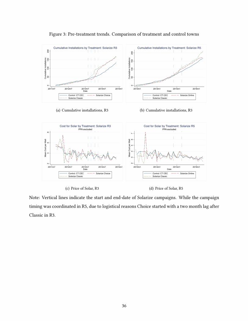
Figure 3: Pre-treatment trends. Comparison of treatment and control towns

050

100

150

200

Cum

ulat

ive

inst

alla

tions

2011m7 2012m7 2013m7 2014m7 2015m7Date

Control: CT CEC Solarize ChoiceSolarize Classic

Cumulative Installations by Treatment: Solarize R3

(a) Cumulative installations, R3

050

100

150

200

Cum

ulat

ive in

stal

latio

ns

2013m1 2014m1 2015m1 2016m1Date

Control: CT CEC Solarize OnlineSolarize Classic

Cumulative Installations by Treatment: Solarize R5

(b) Cumulative installations, R3

24

68

Mea

n C

ost p

er W

att

2011m7 2012m7 2013m7 2014m7 2015m7Date

Control: CT CEC Solarize ChoiceSolarize Classic

PPA excludedCost for Solar by Treatment: Solarize R3

(c) Price of Solar, R3

23

45

67

Mea

n Co

st p

er W

att

2013m1 2014m1 2015m1 2016m1Date

Control: CT CEC Solarize OnlineSolarize Classic

PPA excludedCost for Solar by Treatment: Solarize R5

(d) Price of Solar, R5

Note: Vertical lines indicate the start and end-date of Solarize campaigns. While the campaign

timing was coordinated in R5, due to logistical reasons Choice started with a two month lag after

Classic in R3.

36

Table 1: Market concentration: active installers and HHI

Pre During Post Pre During Post Pre During PostNumb.installers/town 2.400 3.447 4.678 4.680 6.172 7.742 4.088 4.328 4.775HHI(normalized) 0.355 0.211 0.244 0.100 0.185 0.163 0.132 0.630 0.195

None Choice Classic

a) Round 3

Pre During Post Pre During Post Pre During PostNumb.installers/town 6.501 5.201 6.063 6.421 9.288 8.935 5.102 5.975 5.537HHI(normalized) 0.159 0.231 0.183 0.193 0.104 0.106 0.277 0.376 0.100

None Online Classic

b) Round 5

Note: Active installers per municipality and mean of normalized HerVndhal-Hirschman Index

(HHI) in Vve-month periods pre-, during- and post-Solarize.

37

Figure 4: Mean price of solar, by type of Vnancing

01

23

45

Mea

n pr

ice

/ Wat

t

Classic Choice NoSolarize campaign

Lease

01

23

45

Mea

n pr

ice

/ Wat

t

Classic Choice NoSolarize campaign

Loan

01

23

45

Mea

n pr

ice

/ Wat

t

Classic Choice NoSolarize campaign

PPA

01

23

45

Mea

n pr

ice

/ Wat

t

Classic Choice NoSolarize campaign

Purchase

Note: Mean solar prices in 5-month intervals. Bar 1 in each group refers to the 5-month period pre-Solarize.Bar 2 to the 5 months of the campaign. Bar 3 to the 5-month period afterwards. Control towns did not participate in any Solarize campaigns (55 Clean Energy Communities).

Price of Solar (R3) by Type of Financing

a) Round 3: Classic, Choice and Control

01

23

45

Mea

n pr

ice /

Wat

t

Classic Online NoSolarize campaign

Lease

01

23

45

Mea

n pr

ice /

Wat

t

Classic Online NoSolarize campaign

Loan

01

23

45

Mea

n pr

ice /

Wat

t

Classic Online NoSolarize campaign

PPA

01

23

45

Mea

n pr

ice /

Wat

t

Classic Online NoSolarize campaign

Purchase

Note: Mean solar prices in 5-month intervals. Bar 1 in each group refers to the 5-month period pre-Solarize.Bar 2 to the 5 months of the campaign. Bar 3 to the 5-month period afterwards. Control towns did not participate in any Solarize campaigns (45 CT Clean Energy Communities).

Price of Solar (R5) by Type of Financing

b) Round 5: Classic, Online and Control

38

Figure 5: Mean price of solar, by focal installer

34

5M

ean

pric

e / W

att

Classic: F Classic: NF Choice: F Choice: NF NoSolarize campaign

Note: Mean solar prices in 5-month intervals. Bar 1 in each group refers to the 5-month period pre-Solarize.Bar 2 to the 5 months of the campaign. Bar 3 to the 5-month period afterwards. All type of residential solarsystems included. Control towns did not participate in Solarize campaigns (55 Clean Energy Communities).F: Focal (selected) installer, NF: Non-focal installer.

Focal vs. Non-focal installersPrice of Solar: Round 3

a) Round 3: Classic, Choice and Control

34

5M

ean

price

/ W

att

Classic: F Classic: NF Online: F Online: NF NoSolarize campaign

Note: Mean solar prices in 5-month intervals. Bar 1 in each group refers to the 5-month period pre-Solarize.Bar 2 to the 5 months of the campaign. Bar 3 to the 5-month period afterwards. All residential solar systemsincluded. Control towns did not participate in Solarize campaigns (45 Clean Energy Communities).F: Focal (selected) installer, NF: Non-focal installer.

Focal vs. Non-focal installersPrice of Solar: Round 5

b) Round 5: Classic, Online and Control

39

Table 2: Main price eUects of Solarize

R3: Classic & Choice R5: Classic & Online

(1) (2) (3) (4)

Solarize Classic –0.543∗∗∗ (0.127) –0.292∗∗ (0.135) –0.136∗ (0.071) 0.146 (0.088)

Solarize Choice/Online –0.634∗∗∗ (0.095) –0.491∗∗∗ (0.086) –0.279∗∗∗ (0.073) 0.004 (0.077)

Post Classic 0.008 (0.113) 0.123 (0.121) –0.190∗ (0.102) 0.004 (0.070)

Post Choice/Online –0.106 (0.145) –0.159 (0.105) –0.256∗∗ (0.115) –0.177∗∗ (0.084)

Observations 4255 4038 4402 4401

R2 0.151 0.308 0.169 0.405

Month FE Y Y Y Y

Municipality FE Y Y Y Y

Controls N Y N Y

Note: Estimation of model speciVcation (5) by OLS. Control variables include system size, type of system mounting

and type of system Vnancing.

Table 3: Robustness: Randomization Inference

Sample Coefficient SE(clustered) c p-value Coefficient SE(clustered) c p-value

Round3Classic&Control -0.291 0.162 108 0.108 0.102 0.122 760 0.76

Choice&Control -0.444 0.122 27 0.027 -0.123 0.099 270 0.27

Choice&Classic -0.312 0.144 72 0.072 -0.246 0.140 59 0.059

Round5Classic&Control 0.148 0.069 784 0.784 0.028 0.066 529 0.529

Online&Control 0.013 0.061 426 0.426 -0.156 0.108 168 0.168

Online&Classic -0.112 0.071 60 0.06 -0.166 0.079 70 0.07

PooledClassic&Competition -0.354 0.074 17 0.017 -0.332 0.072 6 0.006

RandomInferencewithn=1000MonteCarlosimulations.Treatmentrandomlyassignedatmunicipalitylevel.

Lefttailedteststatistic,c=numberofcasesinwhichthesimulatedregressioncoefficientissmallerthanthetrueone.

P-valuesarecalculatedasp=c/n.ThepooledsamplecombinestheClassicmunicipalitiesfromRound3andRound5,

andtestsfortheNullHypothesisofequaltreatmenteffects:Singleinstaller(Classic)vs.Competition(ChoiceandOnline).

Solarize PostSolarize

40

Table 4: Main quantity eUects of Solarize: R3

R3: Classic & Choice R5: Classic & Online

(1) (2) (3) (4)

Solarize Classic 4.517∗∗∗ 4.562∗∗∗ 5.484∗∗∗ 5.572∗∗∗

(1.028) (1.060) (1.208) (1.120)

Solarize Choice/Online 6.080∗∗∗ 5.835∗∗∗ 2.922∗ 3.119∗∗

(1.186) (1.230) (1.530) (1.446)

Post Classic –1.381∗∗∗ –0.925∗∗∗ 0.542 0.538

(0.345) (0.311) (1.253) (1.165)

Post Choice/Online –0.860∗ –0.420 –0.057 0.088

(0.434) (0.429) (0.945) (0.875)

Observations 4001 4001 3129 3129

R2 0.386 0.459 0.486 0.535

Month FE Y Y Y Y

Municipality FE Y Y Y Y

41

Figure 6: Price dynamics

-2-1

.5-1

-.50

.5C

ost p

er W

att

-8 -4 0 4 8 12 16Month (relative to Solarize)

Classic ChoiceControl

a) Round 3. Months relative to Solarize campaign.

-1.5

-1-.5

0.5

1Co

st p

er W

att

-8 -4 0 4 8 12 16Month (relative to Solarize)

Classic OnlineControl

b) Round 5. Months relative to Solarize campaign.

Note: The Vgure displays point estimates and 95% conVdence intervals for campaign × time dummies to show the

dynamic impact of Solarize on equilibrium prices. Regression follows main speciVcation (5) but includes a campaign

× time dummy (2-month periods). Time t-1 omitted from the regression. The vertical lines indicate the duration of

the Solarize campaigns.

42

Figure 7: Quantity dynamics

-50

510

15In

stal

latio

ns

-8 -4 0 4 8 12 16Month (relative to Solarize)

Classic ChoiceControl

a) Round 3: Months since start of Solarize campaign.

-50

510

15In

stal

latio

ns

-8 -4 0 4 8 12 16Month (relative to Solarize)

Classic OnlineControl

b) Round 5: Months since start of Solarize campaign.

Note: Plot displays coeXcients and 95% conVdence intervals for campaign × time dummies to show the dynamic

impact of Solarize campaigns on equilibrium quantities. Regression follows main speciVcation (6) but includes a

dummy for every 2-month period. Time t-1 omitted from the regression. The vertical lines indicate the duration of

the Solarize campaigns.

43

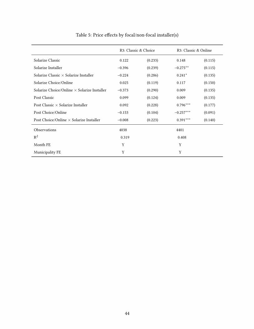
Table 5: Price eUects by focal/non-focal installer(s)

R3: Classic & Choice R3: Classic & Online

Solarize Classic 0.122 (0.233) 0.148 (0.115)

Solarize Installer –0.396 (0.239) –0.275∗∗ (0.115)

Solarize Classic × Solarize Installer –0.224 (0.286) 0.241∗ (0.135)

Solarize Choice/Online 0.025 (0.119) 0.117 (0.150)

Solarize Choice/Online × Solarize Installer –0.373 (0.290) 0.009 (0.135)

Post Classic 0.099 (0.124) 0.009 (0.135)

Post Classic × Solarize Installer 0.092 (0.228) 0.796∗∗∗ (0.177)

Post Choice/Online –0.153 (0.104) –0.257∗∗∗ (0.091)

Post Choice/Online × Solarize Installer –0.008 (0.223) 0.391∗∗∗ (0.140)

Observations 4038 4401

R2 0.319 0.408

Month FE Y Y

Municipality FE Y Y

44

Figure 8: SolarCity market shares

0.2

.4.6

.81

Mar

ket S

hare

R3 Choice R3 Classic R3 Control R5 Online R5 Classic R5 ControlSolarize campaign

Note: Mean market share of SolarCity in 5-month intervals relative to Solarize. Bar 1 in each group refers tothe 5-month period pre-Solarize. Bar 2 to the 5-month period post Solarize. Control towns did not participatein any campaign (CT Clean Energy Communities).

Market share SolarCity: Pre/Post Campaign

Note: SolarCity market shares: 5-month pre- and post-Solarize. Individual campaigns. Zero market shares imputed

in case there are no sales in a given market (5-month interval × municipality).

45

10 Appendix

Description of the CT Solar Market

CT has a small, but fast-growing market for solar PV, which has expanded from only three

installations in 2004 to nearly 7,200 installations in 2015. Despite this, the cumulative number

of installations remains a very small fraction of the potential; nowhere in CT is it more than 5

percent of the potential market and in most municipalities it is less than 1 percent.44 The pre-

incentive price of a solar PV system has also dropped substantially in the past decade, from an

average of $8.39/W in 2005 to an average of $4.44/W in 2014 (Graziano and Gillingham 2015).

Despite being in the Northeastern United States, the economics of solar PV in CT are sur-

prisingly good. While CT does not have as much sun as other regions, it has some of the highest

electricity prices in the United States. Moreover, solar PV systems in CT are eligible for state re-

bates, federal tax credits, and net metering.45 For a typical 4.23 kW system in 2014, we calculate

that a system purchased with cash in southern CT would cost just under $10,000 after accounting

for state and federal subsidies and would have a internal rate of return of roughly 7 percent for a

system that lasts 25 years. From a private consumer perspective, solar PV systems are very often

an ex ante proVtable investment. This is important in the context of this study, for it indicates

that Solarize campaigns are nudging consumers towards generally proVtable investments. There

of course will be heterogeneity in the suitability of dwellings for solar PV.

During the time period of this study, the CT solar market had approximately 90 installers,

ranging in size from small local companies to large national installers. The state rebates, dis-

bursed by the CGB, began in 2006 at $5.90 per W and declined to $1.75 per W by the end of

2014. The incentives were held constant during the time periods covered by the treatments in

this study. The CT solar market has been slow to adopt third party-ownership (e.g., solar leases

or power purchase agreements) and most systems have been purchased outright.46

44Estimates based on authors’ calculations from solar installation data and potential market data based on satellite

imaging from Geostellar (2013).45Net metering allows excess solar PV production to be sold back to the electric grid at retail rates, with a calcu-

lation of the net electricity use occurring at the end of each month. Any excess credits remaining on March 31 of

each year receive a lower rate.46As of 2014, roughly 37 percent of all systems installed were third party-owned, and these third party-owned

systems were distributed across CT and not concentrated in any particular municipalities.

46

Table A.1: Solarize municipalities

ROUND3

R3Classic StartDate EndDate InstShare

SolarCityShareFocal Inst

ShareSolarCity

ShareFocal Inst

ShareSolarCity

ShareFocal

Ashford 9/24/13 2/11/14 7 57.14 14.29 23 8.7 91.3 7 57.14 14.29Chaplin 9/24/13 2/11/14 3 0 33.33 14 0 100 2 100 0Easton 9/22/13 2/9/14 4 50 25 12 0 100 5 40 40Greenwich 10/2/13 2/18/14 6 16.66 33.33 38 5.26 94.74 9 44.44 44.44Hampton 9/24/13 2/11/14 2 0 50 13 7.69 76.92 1 0 100Manchester 10/3/13 2/20/14 11 36.36 0 47 6.38 82.98 21 66.67 33.33Newtown 9/24/13 2/28/14 5 60 40 33 0 96.97 13 30.77 23.08Pomfret 9/24/13 2/11/14 7 28.57 57.14 8 0 100 2 0 100Redding 9/22/13 2/9/14 1 0 0 9 0 77.78 2 50 50Trumbull 9/22/13 2/9/14 2 0 0 45 4.44 80 11 27.27 9.09WestHartford 9/30/13 2/18/14 9 44.44 22.22 64 6.25 89.06 33 42.42 33.33

R3ChoiceCheshire 11/14/13 4/8/14 4 25 0(0) 43 6.98 90.7(3) 25 32 40(3)Columbia 11/4/13 3/25/14 1 0 0(0) 27 3.7 92.59(3) 6 33.33 0(0)Enfield 11/20/13 4/15/14 7 57.14 28.6(2) 62 12.9 77.42(3) 32 75 12.5(2)Lebanon 11/4/13 3/25/14 0 0 0(0) 37 5.41 94.59(3) 6 66.67 16.67(1)Stamford 11/21/13 4/15/14 7 28.57 14.29(1) 22 4.55 81.82(3) 23 41.67 16.67(1)WestHaven 11/13/13 4/8/14 6 33.33 0(0) 15 6.67 86.67(2) 29 20.69 27.59(2)

DURING5MONTHPRE 5MONTHPOST

ROUND5

R5Classic StartDate EndDate InstShare

SolarCityShareFocal Inst

ShareSolarCity

ShareFocal Inst

ShareSolarCity

ShareFocal

Burlington 11/19/14 4/9/15 13 23.08 0 58 8.62 77.59 12 41.67 16.67EastGranby 12/2/14 4/22/15 8 25 50 27 33.33 62.96 10 40 0NewCanaan 12/2/14 4/22/15 5 60 0 16 0 100 5 20 40NewHartford 11/17/14 4/7/15 10 50 0 23 21.74 60.87 18 38.89 11.11Suffield 12/2/14 4/22/15 22 72.73 13.64 61 19.67 60.66 23 47.83 8.7Windsor 12/2/14 4/22/15 21 66.67 4.76 58 31.03 63.79 35 45.71 8.57WindsorLocks 12/2/14 4/22/15 19 84.21 0 42 30.95 52.38 18 33.33 22.22

R5OnlineLyme 11/18/14 4/8/15 3 0 66.66(2) 6 0 100(3) 1 0 100(1)OldLyme 12/4/14 4/24/15 8 37.5 37.5(3) 24 8.33 75(5) 9 22.22 44.44(4)SouthWindsor 11/10/14 3/31/15 33 66.67 18.18(3) 43 27.91 60.48(6) 37 35.14 22.04(5)Woodstock 12/3/14 4/23/15 13 53.85 15.38(2) 32 31.25 56.23(5) 15 33.33 26.67(2)

5MONTHPOSTDURING5MONTHPRE

Note: The above tables list all municipalities participating in Solarize round 3 (Classic and Choice) and round 5

(Classic and Online). They show the total number of installations (inst) in 5-month intervals relative to the Solarize

campaign as well as the market shares of SolarCity and the focal (Solarize) installer(s). In the case of Choice and

Online, the number of active focal installers is annotated in parenthesis. We label an installer as active if he has

made at least one sale in the 5-month period in a given market.

47

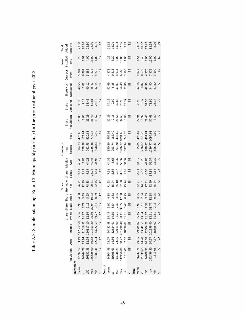
TableA.2:S

amplebalancing:

Rou

nd3.Mun

icipality(m

eans)for

thepre-treatm

enty

ear2012.

Popu

latio

nArea

Income

Share

White

Share

Black

Share

Asian

Share

Homeo

wne

rShare

5bed

sMed

ian

Age

Num

bero

fne

w

houses

Fees

Share

Repu

blican

Share

Democrat

ShareNot

Registered

Costper

Watt

New

Installati

ons

Total

Adde

dcapacity

Treatm

ent

mean

32992.17

33.49

117362.50

85.36

5.90

4.88

76.21

9.61

43.46

804.73

473.60

25.05

33.30

40.55

5.281

5.29

27.30

sd34444.76

13.24

31016.55

11.77

6.72

3.35

12.39

5.43

3.85

178.28

173.61

6.01

7.19

5.02

0.794

3.92

20.36

p50

26932.33

32.24

114317.10

92.34

2.15

3.65

78.13

9.15

44.29

762.93

420.88

25.29

31.42

40.11

5.285

4.00

22.30

max

125885.00

59.38

191353.80

96.89

22.94

10.22

90.21

22.26

49.48

1235.48

777.35

36.49

52.81

48.47

7.675

16.00

72.30

min

1683.41

12.04

73222.59

59.77

0.16

0.69

52.45

1.54

34.96

558.83

9.99

13.62

26.15

32.15

4.270

1.00

4.01

N17

1717

1717

1717

1717

1717

1717

1717

1717

Control

mean

24804.58

28.07

94482.88

85.48

5.90

4.18

71.63

7.51

44.39

950.20

504.02

22.29

34.19

42.69

4.878

4.29

21.62

sd30798.69

14.36

32684.61

14.65

8.54

2.82

15.04

5.56

5.66

293.74

182.49

7.16

9.99

6.25

0.613

3.29

18.01

p50

14048.29

23.55

92111.90

91.71

2.40

3.65

75.10

5.97

45.37

901.20

437.69

21.68

32.86

43.01

4.931

3.00

14.93

max

142456.80

60.27

201298.40

98.11

39.77

12.38

92.50

34.96

55.37

1786.771094.68

37.63

73.96

54.40

6.660

16.00

92.65

min

1313.05

7.67

38598.02

31.81

0.43

0.25

25.24

1.66

31.32

587.34

248.75

3.80

23.37

21.80

3.190

1.00

2.79

N55

5555

5555

5555

5555

5555

5555

5552

5252

Total

mean

26737.76

29.35

99885.02

85.45

5.90

4.35

72.71

8.01

44.17

915.85

496.84

22.94

33.98

42.18

4.977

4.54

23.02

sd31639.65

14.20

33541.59

13.94

8.10

2.94

14.51

5.57

5.28

276.87

179.70

6.97

9.37

6.02

0.679

3.45

18.62

p50

14408.93

26.68

92604.22

91.87

2.38

3.65

77.51

6.50

44.86

888.87

437.61

22.41

32.56

42.95

4.970

3.00

17.42

max

142456.80

60.27

201298.40

98.11

39.77

12.38

92.50

34.96

55.37

1786.771094.68

37.63

73.96

54.40

7.675

16.00

92.65

min

1313.05

7.67

38598.02

31.81

0.16

0.25

25.24

1.54

31.32

558.83

9.99

3.80

23.37

21.80

3.190

1.00

2.79

N72

7272

7272

7272

7272

7272

7272

7269

6969

48

TableA.3:S

amplebalancing:

Rou

nd5.Mun

icipality(m

eans)for

thepre-treatm

enty

ear2013.

Popu

latio

nArea

Income

Share

White

Share

Black

Share

Asian

Share

Homeo

wne

rShare

5bed

sMed

ian

Age

Num

bero

fne

w

houses

Fees

Share

Repu

blican

Share

Democrat

ShareNot

Registered

Costper

Watt

New

Installati

ons

Total

Adde

dcapacity

Treatm

ent

mean

13239.07

30.97

93764.69

84.11

7.65

5.25

81.84

10.93

46.25

847.96

492.08

28.99

29.59

39.81

4.648

6.45

37.93

sd9308.06

14.15

28503.81

15.44

13.22

3.07

5.82

7.22

5.17

216.95

111.43

7.56

6.80

4.18

0.337

3.45

20.22

p50

10388.22

30.15

87689.51

86.25

3.56

3.31

82.94

9.16

44.80

836.93

472.00

29.66

27.52

39.80

4.695

6.00

32.72

max

32515.20

62.09

159172.40

95.98

46.44

10.06

94.09

26.54

58.99

1283.11

778.72

43.23

48.78

47.20

5.095

11.00

60.11

min

2586.59

7.93

48797.09

41.53

0.31

1.85

72.97

1.63

39.49

571.78

364.00

14.13

24.51

31.06

3.940

1.00

3.88

N11

1111

1111

1111

1111

1111

1111

1111

1111

Control

mean

12949.68

28.49

89486.90

89.25

3.42

4.73

73.18

8.96

46.46

1095.26

434.79

24.52

31.53

43.01

4.661

6.04

33.33

sd10183.06

15.06

32963.19

6.47

3.56

3.35

10.86

7.17

5.32

415.95

137.76

6.02

6.36

5.24

0.504

5.78

31.65

p50

10445.95

23.55

80791.41

90.90

2.65

4.18

75.65

7.67

46.52

1002.12

392.51

23.35

30.96

43.57

4.674

4.00

21.59

max

34523.67

60.27

180719.30

98.46

23.70

14.14

91.69

44.44

60.46

2174.59

773.04

38.40

51.82

53.64

6.247

32.00

171.99

min

1283.64

7.67

42867.96

59.95

0.60

0.27

32.48

1.63

32.50

621.22

224.00

13.09

22.00

33.25

3.510

1.00

3.80

N45

4545

4545

4545

4545

4545

4545

4545

4545

Total

mean

13006.53

28.97

90327.18

88.24

4.25

4.84

74.88

9.35

46.42

1046.68

446.04

25.40

31.15

42.38

4.658

6.13

34.23

sd9935.89

14.80

31936.18

9.00

6.69

3.27

10.61

7.16

5.24

395.98

134.04

6.53

6.43

5.18

0.473

5.38

29.65

p50

10417.09

26.68

82901.77

90.82

2.69

3.94

76.43

7.97

46.18

977.45

412.00

24.18

28.93

42.67

4.683

4.00

24.02

max

34523.67

62.09

180719.30

98.46

46.44

14.14

94.09

44.44

60.46

2174.59

778.72

43.23

51.82

53.64

6.247

32.00

171.99

min

1283.64

7.67

42867.96

41.53

0.31

0.27

32.48

1.63

32.50

571.78

224.00

13.09

22.00

31.06

3.510

1.00

3.80

N56

5656

5656

5656

5656

5656

5656

5656

5656

49

Figure A.1: Histogram of main dependent variables

0.2

.4.6

.8De

nsity

2 4 6 8 10 12Cost

Note: Distribution of the cost of solar for treatment and control towns in Round 3. The sample is limited toOctober 2011 to May 2015.

(a) Price of solar, sample R3

0.2

.4.6

.8D

ensi

ty

0 5 10 15Cost

Note: Distribution of the cost of solar for treatment and control towns in Round 5. The sample is limited toDecember 2012 to December 2015.

(b) Price of solar, sample R5

0.1

.2.3

.4.5

Den

sity

0 10 20 30 40Number of new installations

Note: Distribution of new solar installations. R3 Sample.

(c) Number of new installations, sample R3

0.2

.4.6

Den

sity

0 10 20 30Number of new installations

Note: Distribution of new solar installations. R5 Sample.

(d) Number of new installations, sample R5

Table A.4: Robustness: Randomization Inference with and without Group Pricing

Sample Coefficient SE(clustered) c p-value Coefficient SE(clustered) c p-valueRound5Online&Control 0.013 0.061 452 0.452 -0.156 0.108 170 0.17Prime&Control 0.011 0.072 475 0.475 -0.129 0.122 203 0.203Online&Prime 0.025 0.048 612 0.612 -0.002 0.151 500 0.5Note:RandomizationInferencewithn=1000MonteCarlosimulations.Treatmentrandomlyassignedatmunicipalitylevel.Lefttailedteststatistic,c=numberofcasesinwhichthesimulatedregressioncoefficientissmallerthanthetrueone.P-valuesarecalculatedasp=c/n.Thecoefficientsin"Online&Prime"refertoOnlineastreatmentassignment.

Solarize PostSolarize

50

Figure A.2: Financing shares by focal installer

0.2

.4.6

.81

No R3_Choice R3_Classic No R3_Choice R3_Classic1 2 3 1 2 3 1 2 3 1 2 3 1 2 3 1 2 3

0 1

Lease LoanPPA Purchasen/a

Fina

ncin

g sh

ares

Graphs by solarize_installer

a) Round 3: Financing shares by type of campaign and focal installer.

0.2

.4.6

.81

No R5_Classic R5_Online No R5_Classic R5_Online1 2 3 1 2 3 1 2 3 1 2 3 1 2 3 1 2 3

0 1

Lease LoanPPA Purchasen/a

Fina

ncin

g sh

ares

Graphs by solarize_installer

a) Round 5: Financing shares by type of campaign and focal installer.

51

Figure A.3: Mean Vnancing shares

0.2

.4.6

.81

Fina

ncin

g sh

ares

Classic Choice No1 2 3 1 2 3 1 2 3

Note: Mean solar prices in 5-month intervals. Bar 1 in each group refers to the 5-month period pre-Solarize.Bar 2 to the 5 months of the campaign. Bar 3 to the 5-month period afterwards. All type of residential solarsystems included. Control towns did not participate in Solarize campaigns (55 Clean Energy Communities).

Solarize vs. Non-Solarize municipalitiesType of Financing: Round 3

Lease LoanPPA Purchasen/a

a) Round 3: Classic, Choice and Control

0.2

.4.6

.81

Fina

ncin

g sh

ares

Classic Online No1 2 3 1 2 3 1 2 3

Note: Mean solar prices in 5-month intervals. Bar 1 in each group refers to the 5-month period pre-Solarize.Bar 2 to the 5 months of the campaign. Bar 3 to the 5-month period afterwards. All type of residential solarsystems included. Control towns did not participate in Solarize campaigns (45 Clean Energy Communities).

Solarize vs. Non-Solarize municipalitiesType of Financing: Round 5

Lease LoanPPA Purchasen/a

b) Round 5: Classic, Online and Control

52

Figure A.4: System size in Solarize municipalities

0.0

5.1

.15

.2.2

5Ke

rnel

den

sity

0 5 10 15 20System size [kwac]

Pre-Solarize SolarizePost-Solarize

5-month pre/during/post campaignR3 Classic: Systemsize

0.0

5.1

.15

.2.2

5Ke

rnel

den

sity

0 5 10 15 20System size [kwac]

Pre-Solarize SolarizePost-Solarize

5-month pre/during/post campaignR3 Choice: Systemsize

a) Round 3: System size in 5 month intervals relative to Solarize.

0.0

5.1

.15

.2Ke

rnel

den

sity

0 5 10 15 20System size [kwac]

Pre-Solarize SolarizePost-Solarize

5-month pre/during/post campaignR5 Classic: Systemsize

0.0

5.1

.15

.2.2

5Ke

rnel

den

sity

0 5 10 15 20System size [kwac]

Pre-Solarize SolarizePost-Solarize

5-month pre/during/post campaignR5 Online: Systemsize

b) Round 5: System size in 5 month intervals relative to Solarize.

53

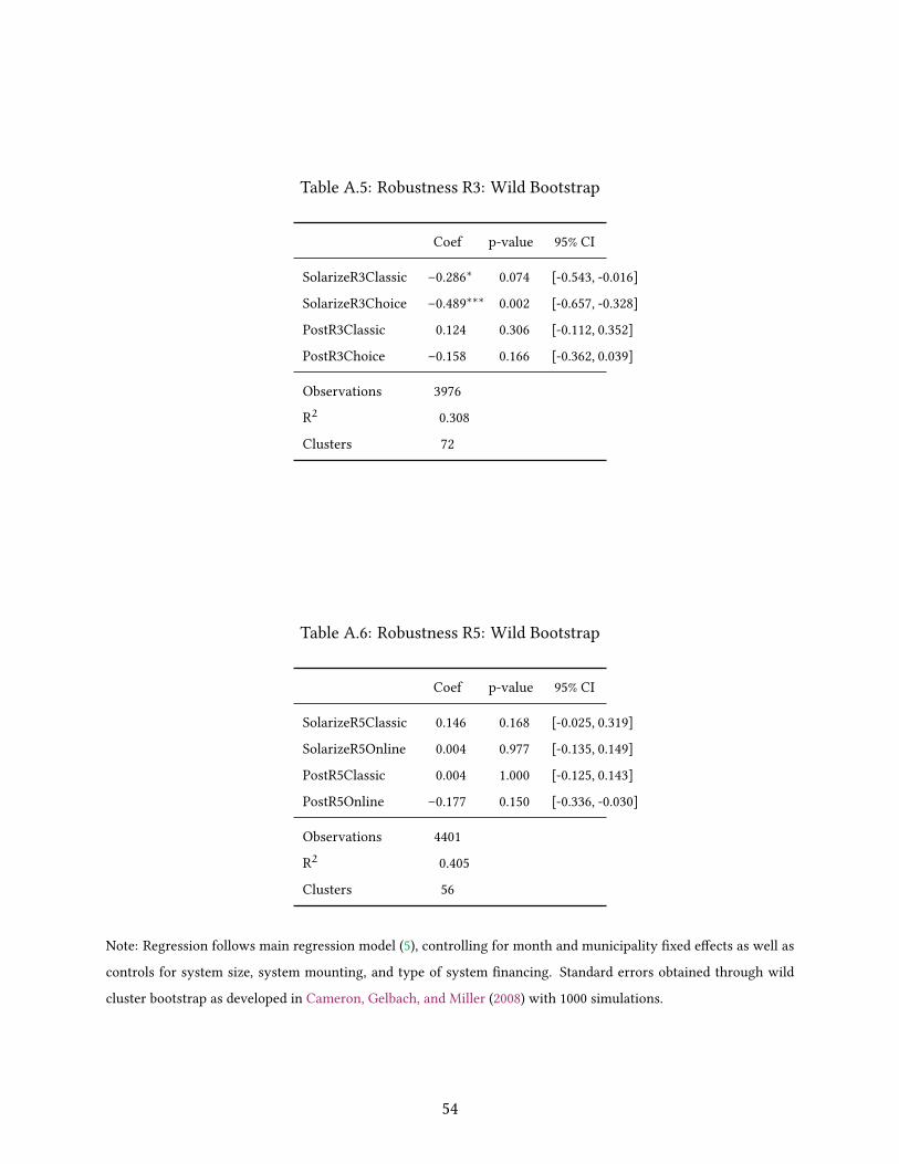
Table A.5: Robustness R3: Wild Bootstrap

Coef p-value 95% CI

SolarizeR3Classic –0.286∗ 0.074 [-0.543, -0.016]

SolarizeR3Choice –0.489∗∗∗ 0.002 [-0.657, -0.328]

PostR3Classic 0.124 0.306 [-0.112, 0.352]

PostR3Choice –0.158 0.166 [-0.362, 0.039]

Observations 3976

R2 0.308

Clusters 72

Table A.6: Robustness R5: Wild Bootstrap

Coef p-value 95% CI

SolarizeR5Classic 0.146 0.168 [-0.025, 0.319]

SolarizeR5Online 0.004 0.977 [-0.135, 0.149]

PostR5Classic 0.004 1.000 [-0.125, 0.143]

PostR5Online –0.177 0.150 [-0.336, -0.030]

Observations 4401

R2 0.405

Clusters 56

Note: Regression follows main regression model (5), controlling for month and municipality Vxed eUects as well as

controls for system size, system mounting, and type of system Vnancing. Standard errors obtained through wild

cluster bootstrap as developed in Cameron, Gelbach, and Miller (2008) with 1000 simulations.

54

Table A.7: R3 (price): sample selection

(1) (2)

SolarizeR3Classic –0.082 –0.283∗∗∗

(0.211) (0.096)

SolarizeR3Choice –0.708∗∗∗ –0.531∗∗∗

(0.198) (0.126)

PostR3Classic 0.135 0.146

(0.253) (0.106)

PostR3Choice –0.304∗∗ –0.158

(0.150) (0.132)

Observations 1185 3853

R2 0.295 0.303

Month FE Y Y

Municipality FE Y Y

Table A.8: R5 (price): sample selection

(1) (2)

SolarizeR5Classic –0.186 0.154

(0.209) (0.095)

SolarizeR5Online –0.378∗∗ 0.075

(0.178) (0.096)

PostR5Classic 0.085 –0.006

(0.169) (0.062)

PostR5Online –0.199 –0.122

(0.155) (0.125)

Observations 1008 4082

R2 0.253 0.389

Month FE Y Y

Municipality FE Y Y

Note: Column 1 limited to purchase-Vnanced installations. Regression controls additionally for system size and

system mounting. Column 2 limits the sample to rooftop installations 6 10 kW and controls for system Vnancing.

55

Table A.9: R3 (quantity): Negative Binomial

(1) (2)

SolarizeR3Classic 3.980∗∗∗ 5.449∗∗∗

(0.647) (0.820)

SolarizeR3Choice 3.076∗∗∗ 5.484∗∗∗

(0.588) (1.477)

PostR3Classic 0.325∗∗∗ 0.355∗∗∗

(0.044) (0.065)

PostR3Choice 0.332∗∗∗ 0.466∗∗∗

(0.054) (0.098)

Observations 4001 4001

Pseudo R2 0.178

Month FE Y Y

Municipality FE Y Y

Table A.10: R5 (quantity): Negative Binomial

(1) (2)

SolarizeR5Classic 2.833∗∗∗ 3.112∗∗∗

(0.350) (0.405)

SolarizeR5Online 2.346∗∗∗ 2.338∗∗∗

(0.396) (0.352)

PostR5Classic 0.979 1.078

(0.117) (0.299)

PostR5Online 0.954 0.939

(0.149) (0.120)

Observations 3129 3129

Pseudo R2 0.250

Month FE Y Y

Municipality FE Y Y

Note: Negative binomial estimation of model (6). The coeXcients can be interpreted as incidence-rate-ratios (IRR). Column 1 estimates the model with XTNBREG and reports standard

errors according to the observed variance-covariance matrix, while Column 2 uses the standardNBREG command with dummy variables to account for municipality Vxed eUects and reports

municipality-clustered standard errors.

56