Policy Research Working Paper 9366

Long-run Returns to Impact Investing in Emerging Market and Developing Economies

Shawn Cole Martin MeleckyFlorian Mölders

Tristan Reed

Development Economics, Development Research GroupFinance, Competitiveness and Innovation Global Practice &International Finance CorporationAugust 2020

Pub

lic D

iscl

osur

e A

utho

rized

Pub

lic D

iscl

osur

e A

utho

rized

Pub

lic D

iscl

osur

e A

utho

rized

Pub

lic D

iscl

osur

e A

utho

rized

Produced by the Research Support Team

Abstract

The Policy Research Working Paper Series disseminates the findings of work in progress to encourage the exchange of ideas about development issues. An objective of the series is to get the findings out quickly, even if the presentations are less than fully polished. The papers carry the names of the authors and should be cited accordingly. The findings, interpretations, and conclusions expressed in this paper are entirely those of the authors. They do not necessarily represent the views of the International Bank for Reconstruction and Development/World Bank and its affiliated organizations, or those of the Executive Directors of the World Bank or the governments they represent.

Policy Research Working Paper 9366

There is interest in impact investing, the idea of deploying capital to obtain both financial and social returns. But pri-vate financial returns are only possible if capital markets are not perfectly integrated, so profit opportunities still exist in certain markets. This proposition is put to the test by exam-ining every equity investment made by one of the largest and longest-operating impact investors across 130 emerg-ing market and developing economies. Since 1961 this

portfolio has performed comparably to public and private equity in the United States, though it has under-performed since 2010. Investments in larger economies have higher returns, and returns decline as banking systems deepen and countries relax capital controls. These results are consistent with a core thesis of impact investing that some eligible markets do not receive sufficient investment capital.

This paper is a joint product of the Development Research Group, Development Economics; the Finance, Competitiveness and Innovation Global Practice; and the International Finance Corporation Economics and Private Sector Development Vice Presidency. It is part of a larger effort by the World Bank to provide open access to its research and make a contribution to development policy discussions around the world. Policy Research Working Papers are also posted on the Web at http://www.worldbank.org/prwp. The authors may be contacted at treed@worldbank.org.

LONG-RUN RETURNS TO IMPACT INVESTING IN

EMERGING MARKET AND DEVELOPING ECONOMIES1

Shawn Cole

Harvard Business School and NBER

Martin Melecky

World Bank

Florian Mölders

International Finance Corporation

Tristan Reed2

World Bank Development Economics Research Group

JEL Classification: F36, G15, O16, O19

Keywords: impact investing, private equity, venture capital, international capital market integration

1We thank Mohan Manem especially for providing an understanding of the data. Seminar participants at the Har-vard Business School Finance Unit, the International Finance Corporation, the World Bank Development EconomicsResearch Group, and the IMF African Department provided helpful comments and questions, along with Adam Fegan,Paddy Carter, Penny Goldberg, Neil Gregory, Victoria Ivashina, Kostas Kollias, Jessica Jeffers, Josh Lerner, Ita MaryMannathoko, Fanele Mashwama, Camilo Mondragón-Vélez, Jacob L. Otto, Tommaso Porzio, Thomas Rehermann,Antoinette Schoar and Jesse Schreger. Anshul Maudar provided excellent research assistance. Cole gratefully ac-knowledges support from the Division of Research and Faculty Development at Harvard Business School. The viewsexpressed in this paper are those of the authors and do not necessarily represent those of the World Bank Group. Allresults have been reviewed to ensure that no confidential information is disclosed.

2Correspondence may be addressed to Tristan Reed, The World Bank, 1818 H Street NW, MC3-317, WashingtonDC 20433. Email: treed@worldbank.org

I. Introduction

There is growing popular interest in impact investing, or deploying financial capital to obtain both

financial as well as (measurable) social or environmental returns. The idea is more controversial

among philosophers, including economists. Brest, Gilson andWolfson (2018) argue that an impact

investor can make a difference in the world by deploying capital3 only if their pursuit of social or

environmental goals leads them to invest in projects that would not have been financed otherwise,

and, if capital markets are perfectly integrated, the impact investor must therefore obtain lower risk-

adjusted returns than traditional investors. An alternative perspective argues that there are frictions

preventing the flow of capital between markets, that commercially-viable projects fail to receive

financing, and that impact investors can promote social objectives while also earning attractive

financial returns.

This paper offers evidence in this debate, through analysis of the cash flows associated with every

equity investment made by the International Finance Corporation (IFC), a member of the World

Bank Group, across 130 emerging market and developing economies (EMDEs). Founded in 1956

with a mandate to “further economic development by encouraging the growth of productive private

enterprise in member countries, particularly in less developed areas,” the IFC’s understanding of

how its investments contribute to improvement in social outcomes is predicated on the view that

some eligible markets do not receive sufficient investment capital. Article I of the charter states

that “the Corporation shall...assist in financing...in cases where sufficient private capital is not

available on reasonable terms.”

The IFC’s history and approach to investing in EMDEs makes its portfolio uniquely suitable for

an investigation of whether certain financial markets offer expected returns that are systematically

higher than others. The portfolio is free from sampling problems such as survivorship bias, and is

more diversified across countries than either foreign direct investment (FDI) inflows or the MSCI

Emerging Market (MSCI EM) index of public equities, both of which have a high concentration3Investors could plausibly affect outcomes in other ways as well, such as by insisting on adherence to environmental,

social or governance (ESG) criteria, which could affect company performance.

2

in the largest economies such as China and Brazil.4 Relative to the market, the IFC also has a

substantially higher share of investment in very poor countries (i.e. those with real GDP per capita

of $1,000 or less).

A principal concern when comparing investment returns across countries is that differences reflect

differences in risk rather than in the risk-adjusted return per se. The data allow us to address this

concern comprehensively. First, since we observe the timing of cash flows we are able to measure

returns in terms of a public market equivalent (PME), which accounts for both the absolute level of

return and the diversification value of payouts that are less correlated with a global risk factor as in

the capital asset pricing model (Kaplan and Schoar, 2005; Sorensen and Jagannathan, 2015). Sec-

ond, since the IFC invests across many sectors, including those considered especially conducive to

economic development such as financial institutions (Levine, 2005) and infrastructure (Aschauer,

1989; Roller and Waverman, 2001), we are able to compare returns across countries within pro-

duction technologies that may vary in their level of non-diversifiable risk. Third, the length of the

time series, the longest in existence of which we are aware, provides assurance that differences in

average returns across countries are not driven by the realization of non-diversifiable country risk

in a few particular years.

The analysis yields three main results. First, ex-post, macroeconomic conditions have material

effects, with a 1 percent increase in cumulative annualized real GDP growth over the life of the

average investment—8 years—associated with an additional 6.62 percentage points of return on

that investment. On the other hand, local currency depreciation worsens the performance, while

local inflation (controlling for the depreciation) is associated with higher returns. There is some

evidence that improvement in sovereign risk during the investment period improves returns.

Second, certain economy-level covariates measured ex-ante, at the time of investment, do predict

performance in a way that is economically and statistically significant: market size and financial

system openness and development. More populous EMDEs have higher mean and median returns4Our paper is related to a few, employing data on the complete portfolio of a single private equity investor: Gompers

and Lerner (1997) study the portfolio of Warberg Pincus and Kerr, Lerner and Schoar (2014) study the portfolio of twoprominent angel investment groups, Tech Coast Angels and CommonAngels.

3

within sectors. Returns fall within economies as they relax capital controls and deepen their bank-

ing sectors. These result are inconsistent with the hypothesis of a perfectly integrated international

capital market, under which expected financial returns are equalized across economies. Quantita-

tively, a less integrated market appears to be more important for returns than economic growth, with

a one standard deviation decrease in financial openness or banking system depth being associated

with an increase in return that is substantially more than is associated with a 1 per-cent increase in

cumulative annualized real GDP growth over the life of the average investment. One potential ap-

proach a development finance institution could take would be to offer subsidies in lesser developed

markets. The finding that the IFC obtains higher returns when capital markets are less developed

supports is not consistent with this approach and suggests the IFC may hold to its mandate to offer

investments on commercial terms.

Third, in pursuing its strategy, the IFC has achieved competitive returns over the long run. Bench-

marking the IFC’s equity investment portfolio to the S&P 500 index (available for our entire sample

period), we calculate that the total portfolio has obtained a PME of 1.15, indicating that the port-

folio has returned 15 percent more over its life than an equivalently timed investment in the public

index would have. Alternative benchmarks yield estimates such as a PME of 1.30 when using the

MSCI EM index (after 1988, when the index becomes available). Returns have been lower for

investments in the most recent decade, with a PME of 0.70 when using the S&P 500 and a PME of

0.98 when using the MSCI EM (IFC’s internal benchmark). Though only 26 percent of these most

recent investments have been realized (and longer holding periods are in these data associated with

higher returns) this decline in portfolio performance is consistent with there being fewer opportu-

nities for financial profit as financial markets have become more developed and open. A broader

lesson is that in the long-run impact investors could find it challenging to deliver persistent returns

at scale when their mandate is to invest in less-integrated markets.

Given that our data include the portfolio of a single investor we do not claim that this performance is

representative of the universe of EMDE private equity investments. Nor is it obvious that any other

asset owner could replicate the IFC’s strategy and returns. The IFC’s membership in the World

Bank Group for instance offers it protection from expropriation not available to other investors.

4

Nonetheless, given it is the only international investor with a portfolio spanning such a large and

diverse set of countries and because it co-invests with a number of funds, the portfolio provides a

unique view of the return to private investment in EMDEs.

Our paper ties together three strands of literature from finance, development economics, and in-

ternational macroeconomics. First, we add to the understanding of the financial return to private

equity investments in general, and impact investing in particular. While the U.S. private equity

industry has been well studied (see Kaplan and Sensoy, 2015, for a comprehensive review) there

is very little rigorous evidence available on returns in EMDEs. Lerner, Sorensen, and Stromberg

(2009) provide an important exception: they use data from Capital IQ to construct a database of

private equity investments around the world starting in about 1990. The authors find that emerging

markets comprise a small fraction of total private equity investment, and that country characteris-

tics have some influence on whether funds pursue strategies of financial engineering, governance

engineering, and/or operational engineering. While they are unable to measure returns, they ex-

amine exits, and find a lower likelihood of success in wealthier countries, and that deals that are

undertaken in “hot” markets are more likely to fail. Our paper contributes to this literature by a)

providing a history of time series over twice as long, and b) providing the first systematic evidence

of returns relative to a benchmark (PME) free of survivorship bias.

A smaller and more recent literature examines the performance of impact investing strategies. Im-

pact investors are defined as those employing a distinctive strategy that contracts on social-benefit

outcomes regardless of their returns target (Geczy, Jeffers, Musto, and Tucker, 2021) or as those

willing to “pay” for externalities by accepting a below-market return (Barber, Morse, and Yasuda,

2020). We offer the first estimate of the long-run return to an impact investing strategy seeking to

provide capital to eligible projects that would not have otherwise received sufficient funding due

to imperfectly integrated financial markets.

Second, the portfolio provides the most comprehensive microeconomic evidence yet on the long-

standing macroeconomic question of whether international credit frictions exist and their quanti-

tative implications for economic development (Feldstein and Horioka, 1980; Lucas, 1990; Alfaro,

5

Kalemli-Özcan and Volosovych, 2008; Chari and Rhee 2020). Previous studies of capital market

integration have found high cross-country covariance in the return to public equities (Campbell

and Hamao, 1992; Harvey, 1995) and a common marginal product of capital implied by the na-

tional accounts in a cross section of countries (Caselli and Feyrer, 2007), concluding that markets

appear well integrated and that there are limited barriers to capital moving between countries. In

contrast, we examine the return to financial capital in private equity transactions and find evidence

of a market segmented by financial sector development, openness and size. Our results, which rely

on firm-level data from a much larger sample of economies (including the very poorest), indicate

that many firms of the size that typically receive foreign direct investment have faced constraints

in finding capital.5

Third, we add to an empirical literature on macroeconomic risk through the analysis of the re-

lationship between key macroeconomic variables and private equity returns. Given that equity

investments represent real assets, economic theory suggests that equity investments may be used

as a hedging instrument against unexpected inflation, and we should therefore expect a positive

correlation between performance and inflation. Exchange rate movements are also expected to im-

pact equity returns such as in the case of exporting firms whose competitiveness increases when

the home currency depreciates. However in the empirical literature there is some evidence of a

negative correlation between equity returns and depreciation (Hau and Rey, 2006). Sovereign risk

ratings, which approximate a set of macroeconomic risk factors, have shown to be negatively cor-

related with equity returns as shown for a set of countries by Brooks et al. (2004) and in the case

of Argentina by Hébert and Schreger (2017).

The paper proceeds as follows: Section II provides a conceptual framework, defining impact in-

vesting in relation to the model of imperfect international capital market integration offered by the

literature on the macroeconomics of development. Section III provides background on the IFC’s

strategy and operations, the equity portfolio data, and reviews the PME methodology for the mea-

surement of financial returns at the portfolio and investment (firm) level. Section IV describes5The average size of a transaction in the IFC’s equity portfolio was $19.5 million in the most recent decade. Ar-

guments in favor of credit frictions have relied on variable or excessively high marginal products of capital at the firmlevel among enterprises with assets less than $400,000 within a single EDME (Banerjee and Duflo, 2014).

6

the IFC’s allocations and summarizes portfolio and individual investment performance. Section

V reports the main evidence on international capital market integration using the framework of

Section II. Section VI shows the evidence on associations of returns and macroeconomic variables

and investment duration. Section VII concludes with reference to recent trends in emerging market

equity performance, and provides policy advice for private and public sectors.

II. Conceptual Framework

In practice, impact investors distinguish themselves from traditional investors through verifiable ef-

fort towards both financial profit and social-benefit objectives.6 Geczy, Jeffers, Musto, and Tucker

(2021) describe how a sample of private impact investment funds contract with employees and

portfolio companies. The IFC was created in order to advance economic development and was one

of the first to measure social outcomes associated with its investments, and also identifies as an

impact investor.7 Though the origin of the term “impact investing” is dated around 2007 the con-

cept is much older: Around the year 200 Rabbi Shimon ben Lakish is reported to have said, with

regards to helping a needy person, that “a loan is greater than a donation, and a business partnership

is greater than all of them” (Levine, 2010, p.291).

The investor’s intent to create a social-benefit does not imply the investor creates one. Brest, Gilson

and Wolfson (2018) argue that an impact investor can make a difference in the world only if they

invest in projects that would not have been financed otherwise (there is term of art for this —

‘additionality’). If impact investors compete with traditional investors for the same deals, it will

be impossible to find such projects. One way to overcome this critique has been to define the

impact investor as an asset owner willing to “pay” for potential positive externalities by taking

below-market returns (Barber, Morse, and Yasuda, 2020). Many impact investors however still

argue they can address social or environmental problems while still earning a competitive financial6The Operating Principles for Impact Management require adherence to an investment process that provides asset

owners with (verifiable) information on the conduct of fiduciaries in pursuit of social-benefit objectives. Signatories tothese Principles include asset managers specialized in “purposeful investing” such as MicroVest Capital ManagementLLC ($287 million in assets under management in accordance with the Principles), legacy private wealth managerssuch as Credit Suisse AG ($4.2 billion), and government-owned development finance institutions such as the EuropeanBank for Reconstruction and Development ($51.7 billion). See https://www.impactprinciples.org/.

7See the foreword by CEO Philippe Le Houérou to IFC (2019a).

7

return; says one “there’s no trade off at all” (Noonan, 2018).

The IFC’s charter proposes a resolution to this inconsistency by offering an alternative definition

of the impact investor: one that provides capital to eligible projects that would not have otherwise

received sufficient funding due to imperfectly integrated financial markets. An impact investor’s

process can make a difference while earning a private financial return only if capital markets are

not perfectly integrated, so profit opportunities still exist in certain markets. The existence of in-

ternational capital market imperfections was a principle on which the World Bank was originally

founded (Clemens and Kremer, 2016). Under this definition, impact investors’ returns could not

be persistent if they are successful in mobilizing capital into less-integrated markets.

In a perfectly integrated international capital market, geography has no systematic effect on the

returns investors receive in exchange for their capital. The null hypothesis is purchasing power

parity in financial returns. If long-run private returns are available in a particular market, investors

will divert their capital there until returns are no longer available (see, e.g., Lucas 1990), either

due to competition that bids up entry multiples, or a decline in the marginal product of capital. An

empirical test of this model is available in the linear regression equation

ri = r0 +X ′c(i)β + εi (1)

where ri is the (risk-adjusted) return on asset i, and r0 is average return on all assets. The vector

X ′c(i) includes various characteristics of country c, where the investment is located. The term εi

is an unrestricted error term. If β ̸= 0 markets are said to be segmented, since the price differs

across capital markets (for a case of international product market segmentation, see Goldberg and

Verboven, 2001). Conversely, if all countries participate in a perfectly integrated capital market

β = 0, and country characteristics would have no effect on the average financial performance of

an investment since all investors receive the same price for their capital. In one leading test of

this hypothesis, Caselli and Feyrer (2007) calculate the marginal product of capital implied by the

national accounts (which is equal to its price in equilibrium) and find it does not vary substantially

across countries, or that β = 0. They conclude that “there is no prima facie support for the view

8

that international credit frictions play a major role in preventing capital flows from rich to poor

countries.”

A thesis of impact investing is that frictions do prevent capital flows between certain markets. For

instance, the manifesto of the Acumen Fund exhorts the fund ”to go where markets have failed.”

The charter of the IFC posits that in some developing countries, commercially-viable projects fail

to receive financing on “reasonable” terms. To make these ideas precise, one could say this thesis

is valid if and only if β ̸= 0. When β = 0 the price of capital is the same everywhere and so capital

must be available in every market on reasonable terms. Conversely, when β ̸= 0 the equilibrium

price of capital is higher in certain markets. If the marginal product of capital diminishes with

scale, moving capital from the market in which the price is lower to the one in which it is higher

will increase welfare. This could be called impact, or making a difference. Estimation of Equation

(1) therefore offers a method to test whether international capital markets are perfectly integrated

and also whether it is possible for an investor to have impact in the way described in IFC’s original

charter.

This conceptual framework shows how economic theory and a cross-section of investments in

different markets are used to test whether it is possible to do well by doing good through welfare-

enhancing arbitrage. This conception of investment impact is consistent with the statements of

many impact investment practitioners, and does not require them to sacrifice return to have an

impact.

The focus of our analysis is variation (and persistence) of returns across geographies within the

portfolio, rather than the total return to the portfolio. Nonetheless, the portfolio return we report

is relevant to a strand of literature concerned with whether impact investment strategies achieve

returns comparable to public benchmarks. Grey et al. (2016) survey 53 impact investing private

equity and venture capital funds, collecting both survey reports of returns and audited financial

statements. Using the Russell Microcap 2000 as a comparator, they estimate that a “pooled end-to-

end aggregate PME calculation for the 170 market-rate-seeking investments in the sample returns

a PME gross of fees, expenses and carried interest of 0.98.” A potential concern with this study is

9

that funds could choose whether to report performance or not; Cochrane (2005) shows that selective

reporting can have important effects on estimates of the returns to venture capital investing. Barber,

Morse, and Yasuda (2020) obtain data from PreQin on 159 impact funds between 1995 and 2014,

and, comparing them to a similar set of non-impact funds, find that impact funds on average achieve

a 4.7 percentage point lower IRR. Their paper focuses on impact investing strategies in general,

rather than seeking to distinguish between funds that seek to obtain market (commercial) returns

and funds that explicitly promise investors lower (concessional) returns. A finding that the average

return for both types of these funds—that is, when pooled together—is below market does not

necessarily indicate that funds seeking market returns obtain below market returns. By analyzing

the portfolio of an investor pursuing economic development and profit goals, we provide the first

estimate of the long-run return to an impact investing strategy that seeks market returns.8

II.A Background on the International Finance Corporation

Through its investments the IFC today seeks to contribute to improvement in social and environ-

mental outcomes aligned with the United Nations’ Sustainable Development Goals (IFC, 2019b).

185 member countries own and govern the institution, determine its policy, and provide equity

capital. The balance sheet size stands at approximately $99 billion, of which $43 billion are

development-related investments and the rest are liquid securities (IFC, 2019c). The carrying value

of the equity investment portfolio comprises 30% of development-related investments.

The IFC charges market-based rates for its loans and seeks market returns on equity investment

(IFC, 2019d).9 The institution’s investment on its own account generally does not exceed 25% of

the value of a project, with other private investors participating through loan syndications, parallel

investments, and other instruments. Given its co-investment with others, we view its portfolio as8All of IFC’s investments may be considered impact investments because they were made with the intent to promote

economic development alongside financial profit, as in the Charter. Defining an impact investor by their objective,rather than their allocation to any particular sector, is how impact investing is defined by the industry itself (see, e.g.,the Operating Principles for Impact Management, GIIN).

9One exception to charging market-based rates comes in the form of a facility for “blended finance” established in2017. Here, IFC capital is blended with concessional capital from donors in order to allow IFC to earn a commercialreturn on an investment that would otherwise not be profitable. Such projects are located exclusively in the poorest(“IDA”) countries, and the decision to include concessional capital is made before the investment is executed. Ourdataset includes four such investments.

10

potentially informative about the returns available to private investors in the markets in which it

operates.

Figure I charts the institution’s financial history in three ratios: return on equity (net income/total

capital), leverage (total assets/total capital) and administrative expense (non-interest expense/total

assets).10 The IFC made its first loan in 1957, providing $2 million to Siemens’ Brazilian affiliate

(IFC, 2018). In 1961, the charter was amended to allow holding equity, leading to a surge in equity

investment during 1963-64 to about 50% of total investment (Kapur et al., 1997).By the end of

the 1960s, this share had decreased to 35%. During the 1980s, the equity share declined to its

lowest level to date at 15%, mainly driven by currency crises and global economic turmoil. At the

beginning of the 1990s, the equity share again increased to around 23%, driven by investments in

the financial sector and infrastructure. This share remained in the mid- 20% range until the Global

Financial Crisis leading to an increase in the share of equity to total investments above 30%.11

Equity investment in private markets has been the basis for growth in the capital base through

retained earnings, with realized gains from these investments leading to high points in return on

equity seen in Panel A in 1989 (RoE = 12.4%) and in 2005 (20.5%).

The IFC also raises funds for its operations at international capital markets. As shown in Panel B,

the IFC’s leverage ratio was 3.6 as at 2019. The extent of borrowing varies substantially across

institutions owned by governments that could also be called impact investors because they seek

to promote economic development through investment in private firms. For instance, the United

Kingdom’s CDCGroup (2019) has a leverage ratio of 1.0, indicating it does not borrow at all, while

the European Investment Bank (2020) has a leverage ratio of 5.8 and the China Development Bank

(2017) has a leverage ratio of 12.9, indicating these banks borrow substantially more relative to

their capital base compared to the IFC today.12

10Values used in calculating these ratios are reported in Appendix Table A.11Figure II discussed in Section IV.A. shows the volume of investment over time.12The CDC Group and the European Investment Bank are signatories to the Operating Principles for Impact Man-

agement, an affirmation that they identify as impact investors. The leverage ratio reported here is total assets dividedby total equity using values from annual reports. For the European Investment Bank, total equity is the sum of accrualsand deferred income, provisions, subscribed capital, reserves, and profit for the financial year.

11

A small literature examines the role of the IFC as an investor and development institution. Dreher et

al. (2019) investigate the link between IFC loan allocation and Boardmembership in the institution,

and find a positive relationship between political influence and lending decisions. Taussig and

Delios (2015) use data from the IFC’s investment in private equity funds to examine the role of local

expertise and performance, finding that local expertise improved performance more in countries

with weak contract enforcement institutions. Kenny, Kalow, and Ramchandaran (2018) analyze

the countries targeted by IFC investment between 2001 and 2016, noting a shift in allocation from

low income countries towards middle-income countries. Neither of these papers reports on the

returns obtained by the IFC. Desai, Kharas and Amin (2017) study the relationship between IFC

project returns and ESG risk factors, though in the period since 2005.

The IFC’s long history and broad geographical diversification allow us to paint an unusually rich

picture of emerging market private equity investment. It is worth, however, noting several caveats.

First, while the IFC’s charter prohibits it from taking government guarantees, the IFC’s affiliation

with the World Bank Group provides additional protection from expropriation. The IFC charter

(Article VI, Section 6) states: “Property and assets of the Corporation, wherever located and by

whomsoever held, shall be immune from search, requisition, confiscation, expropriation or any

other form of seizure by executive or legislative action.” Realized returns subject to this immunity

may not be representative of what is available to independent investors.

Second, Panel C in Figure I shows IFC’s operating expenses at around 2% of assets during 1964-

1988, though they have subsequently declined, and are today approximately 1.4% of assets. These

costs include public policy work, and technical assistance for investments, among other things, and

also investment costs associated with the debt portfolio, which may be lower than for the equity

portfolio alone. Since it is not possible to accurately apportion fixed costs to each investment, and

because the IFC engages in significant non-investment activity, such as research and field-building,

we analyze portfolio and individual investment performance on a gross basis, without subtracting

off operating expenses. Some investments are collective investment vehicles such as private equity

funds.

12

III. Data and Measurement

III.A Investment Financial Performance

The main data used in this study are the complete set of cash flows to and from all 2,509 equity

investments (in companies or funds) beginning at the founding of the IFC in 1956 until June 30th,

2019.13 The IFC’s equity investments are primarily made through the direct purchase of a minority

stake in a company, or participation in a fund as a limited partner. The dataset includes the month

of each cash flow, the exact value in US dollars, and the most recent mark-to-market valuation of

investments that are still held in the portfolio. Each investment’s “vintage year” is defined as the

year of first cash flow to the company. Each company is categorized by the “country-of-risk”, or

the country in which the company generates most of its revenue, as well as by one of 23 sectors

(e.g., electric power, food and beverage, finance and insurance). In Appendix Table B, Panel A

shows the count of investments by decade and geographic region according to the World Bank

Group regional classification and Panel B shows the count of investments by decade and sector.

Included among these investments are IFC’s interests in individual companies acquired through

its participation as a limited partner in funds managed by the IFC Asset Management Corporation

(AMC).14

We use the cash-flows to calculate the financial performance of the entire portfolio as well as of the

investment into each company (or fund). To do this the cash-flow stream is divided into its positive

and negative parts, called distributions (dist (t)) and contributions (cont (t)). Distributions are the

cash flows returned to IFC either through dividend payments or through the sale of the company’s

shares. For investments that are still held in the portfolio, we treat the valuation on June 30, 2019

as a positive distribution, as if the investment is liquidated on that date at its fair value, consistent

with accounting practice (we also explore how sensitive our results are to these fair value marks,

by restricting the sample to only mature investments). Contributions are the IFC’s investments into

the company, including the payment of management fees in cases when the company is a fund.13We focus on cash flows exclusively related to equity investments, and therefore do not include investments that

include both equity and debt components (e.g., convertible loans). We leave analysis of the IFC’s credit investmentsto future research.

14Cash flows between portfolio companies of third-party funds in which IFC is a limited partner are not observed.

13

Our measure of financial return is the Kaplan and Schoar (2005) public market equivalent, defined

by

PME =

∑t

dist(t)1+R(t)∑

tcont(t)1+R(t)

where R(t) is the realized total return of the market index from the year of first cash flow (t = 0)

to the time of the distribution or contribution (t). Sorensen and Jagannathan (2015) motivate the

PME as a method to evaluate returns for a CAPM investor whose wealth is held in the index; if

the ratio is greater than one, the investor prefers the portfolio to the index. We use the S&P 500

index as a market reference for comparability to the literature on private equity performance, and

because the time series is complete back to our first cash flow in 1961. In some results, we use

the MSCI World index and the MSCI Emerging Markets index as alternatives, though these start

later in 1970 and 1988.15 For comparison, we also report a measure of financial return that does

not correct for market risk or the time value of money, total value to paid-in capital, or

TV PI =

∑t dist (t)∑t cont (t)

which is also known as the investment multiple, or multiple of money. Recall that if the investment

has not been fully realized, its fair value on the final date of our data set is treated as a distribution.

It is on this basis that the sum of distributions are called “total value.”

Our dataset allows us to avoid two forms of selection bias that typically hamper analyses of the

performance of an asset class. A first source of selection bias is survivorship bias, such as when

successful investments are more likely to appear in a dataset than failures (Carhart, Carpenter,

Lynch and Mutso (2002) discuss this in the context of the mutual fund industry). Since our dataset

includes all of the IFC’s investments—even thewrite-offs—our analysis will not be affected by such

bias. A second source of selection bias is infrequent valuation, such as when an investor values

investments only upon a successful initial public offering (IPO) or after the company completes a

successive round of fundraising (Cochrane (2005) discusses this in the context of venture capital).

Because valuations are positively correlated with these events, ignoring investments that have not15Index values are as reported by Bloomberg.

14

gone public or raised further funds could also lead to an upward bias in average performance. Our

estimates are not subject to such bias, first because the majority have already exited, and second

because we include the mark-to-market valuations of all unrealized investments on the same date.

To check that our results are not driven by mark-to-market valuations that are difficult to determine

given the youth of the investment, we restrict the sample to only mature investments, by excluding

the 5 most recent vintage years.

III.B Marcoeconomic Covariates

In our analysis we relate returns to a variety of economy-level covariates such as market size,

openness, sovereign risk, and financial development. Two measures of market size, population

and GDP per capita, are taken from the World Development Indicators (World Bank, 2019a). Our

main measure of financial openness is the index of Chinn and Ito (2006, 2008), or the first princi-

pal component of dummy variables codifying capital controls including multiple exchange rates,

restrictions on current account transactions, restrictions on capital account transactions, and regu-

latory requirements to surrender export proceeds as reported in the IMF’s Annual Report on Ex-

change Arrangements and Exchange Restrictions. We complement this index with indicators from

Fernández et. al. (2015) who codify the IMF’s more detailed records, available after 1995, indi-

cating whether foreigners specifically have the right to purchase or sell local equity shares. Our

measures of financial development are the standard measures of private sector credit to GDP, in-

dicating banking sector development, and stock market capitalization to GDP, indicating capital

markets development. Both are reported in the Global Financial Development Database (World

Bank, 2019b).

We also relate returns to several indices used by some investors to assess country risk or investa-

bility: (i) a political risk index of the PRS Group, (ii) the Economic Freedom index of the Heritage

Foundation, (iii) perceptions of corruption by Transparency International, (iv) Economic Fitness,

a dynamic measure of economic complexity that predicts growth (Cristelli et al., 2017), and (v)

the Ease of Doing Business Distance to Frontier measure (World Bank, 2019a). Finally, we relate

15

returns to several macroeconomic variables reported in the World Development Indicators: (i) real

GDP growth, (ii) inflation and (iii) local currency deprecation; (iv) central government debt as a

share of GDP as reported by the IMF as well as (v) a sovereign debt rating index produced by

Oxford Economics based on an average of ratings by Moody’s, S&P and Fitch.

IV. Allocations and Investment Performance

IV.A Location and Timing of IFC’s Equity Investments

First, to provide context for the results on financial performance, we compare the IFC’s equity port-

folio cash deployed (i.e. contributions, as defined above) to FDI inflows reported by the United

Nations Conference on Trade and Development (UNCTAD). FDI inflows are defined as the acqui-

sition of an equity capital stake of 10 percent or more by investors resident in a country different

than the one in which the enterprise is located, and hence include most cross-border private equity

investment, either by funds or through mergers and acquisitions by firms.

Table I reports the country allocation of IFC investment and FDI in constant dollars broken down by

whether countries were classified as “advanced economies” or “emerging market and developing

economies” (EMDEs) by the IMF in 2019. All values are in real terms. Overall, IFC equity invest-

ment accounts for 0.09 percent of total FDI. Unlike FDI however the IFC has been entirely focused

on EMDEs, with 97.7 percent of its cash deployed in current EMDE and 2.3 percent in countries

that have since transitioned to advanced economy status such as the Republic of Korea, Greece

and the Czech Republic. In contrast, 61.3 percent of FDI has gone to advanced economies where

the IFC has never deployed cash, such as the United States (which has received 18 percent of total

FDI), the United Kingdom (6.9 percent) and Hong Kong SAR, China (4.3 percent). The IFC also

has not deployed equity investment in certain jurisdictions through which some FDI into EMDEs is

indirectly channeled (Coppola, Maggiori, Neiman and Schreger, 2020), namely the British Virgin

Islands (2.2 percent of total FDI), the Cayman Islands (1.5 percent), and the United Arab Emirates

(0.4 percent).

16

Figure II shows the value of IFC equity contributions and global FDI inflows for each year in

constant US dollars since 1970, the first year the FDI series is available. Overall, IFC invest-

ment has grown with FDI, and has been less volatile during certain downturns. While global FDI

dropped substantially during the 2001 and 2008 recessions, in 2001 IFC investment actually in-

creased and in 2008—though falling briefly—it grew substantially in subsequent years while global

FDI plateaued. However, the year 2018 did see a large decline in both FDI and equity investment

by the IFC. In 2017, the IFC began pursuing a capital increase from shareholders that was approved

in 2019, suggesting the institution considered itself still capital constrained at that point.

When examining geographic diversification within EMDEs, we find the IFC’s portfolio is more di-

versified compared to FDI. East Asia and the Pacific together with Latin America and the Caribbean

(defined using World Bank regional classifications) attracted 54.0 percent of FDI in EMDEs in

which IFC has invested, whereas only 41.4 percent of IFC’s investment has gone to these regions.

While 11.3 percent of IFC investment has gone to Sub-Saharan Africa, the continent received only

5.3 percent of FDI among countries in which IFC has invested. Looking at the largest FDI destina-

tions in each region, IFC is underweight in China (9.3 percent vs. 19.5 percent of FDI in EMDEs

in which IFC has invested), Brazil (6.5 percent vs. 9.0 percent), Nigeria (1.0 percent vs. 1.1 per-

cent), and Saudi Arabia (0.2 percent vs. 2.3 percent), while it is overweight in India (9.6 percent

vs. 4.3 percent) and the Russian Federation (5.4 percent vs. 4.6 percent). Standard public equity

investment references in EMDEs are even more concentrated than FDI. As of June 2020, more

than 75 percent of holdings in the MSCI Emerging Market stock index were located in just five

economies: China, Taiwan (China), Korea, India, and Brazil. Compared to both public and private

cross-border equity investment in EMDEs, the IFC appears highly diversified.

Kenny, Kalow and Ramachandran (2018) argue that, despite its overall focus on EMDEs, IFC still

has a relatively small allocation towards the poorest countries within the group. This is consistent

with the presence of fewer investable opportunities in smaller economies, where size is measured

by real GDP. The capital asset pricing model (CAPM) predicts that, in equilibrium, each investor

holds the world portfolio. If a country’s investment opportunities are proportional to GDP, the

CAPM investor’s allocation will also be proportional to the country’s GDP, a result consistent with

17

the outsize allocation of FDI to large countries such as the United States and China. Under these

assumptions the appropriate test for whether IFC overweights a particular income group (relative

to the CAPM investor) is whether its allocation to the group is larger as a share of GDP.

Figure III reports average annual FDI inflows/GDP (Panel A), and average annual IFC invest-

ment/GDP (Panel B) as a function of a country’s real per capita income in order to conduct such a

test. The countries in each group vary over time as real GDP per capita grows, so this figure de-

scribes the weighting of investment towards specific income levels rather than specific countries.

Relative to our theoretical CAPM benchmark both types of investment appear to overweigh the

poorest countries. FDI inflows are on average 1.4 percent of GDP in countries with over $10,000

in GDP per capita and 1.9 percent of GDP in countries with less than $1,000 in GDP per capita, or

35 percent more; IFC exhibits a much steeper slope, investing just 0.0002 percent of GDP in coun-

tries with per capita income over $10,000, and 0.0044 percent of GDP in countries with less than

$1,000 in per capita income, or roughly twenty-two times more. IFC also overweights lower mid-

dle income countries (i.e., real GDP per capita of $1,001-$5,000) relative to upper middle income

countries (i.e., real GDP per capita of $5,001-$10,000), whereas FDI is slightly lower as a share of

GDP in lower middle income countries relative to upper middle income countries. Interestingly,

when comparing low income countries (i.e., real GDP per capita <$1,000) to lower middle income

countries, FDI flows relative to GDP are 24 percent greater in low income countries, while the IFC

only invests 1 percent more. An explanation for this may be that, relative to FDI, the IFC is un-

derweight in oil, gas and mining, which comprise the bulk of FDI projects in low income countries

(Dabla-Norris et al., 2010) but may not satisfy certain ESG criteria, or satisfy IFC’s mandate to

invest only in projects that could not secure financing from another source.

A final question is how IFC equity investment is timed, relative to both FDI and lending to national

governments by the World Bank. We investigate this question using a panel vector autoregres-

sion model, in which we regress three country year variables, IFC equity investment/GDP, FDI

inflows/GDP and World Bank commitments/GDP on the values of each variable in the past two

years, as well as dummies for banking, currency and sovereign debt crises as reported by Laeven

and Valencia (2020). The VAR model allows for covariance between the error terms in each of the

18

three regression equations to account for the fact that they may be jointly determined as a market

equilibrium.

Results are reported in Table II, along with the p-values of Chi-squared tests for four instances

of potential Granger causality between the series. The null hypothesis of the first test is that, in

column (1), lagged values of FDI/GDP do not predict IFC/GDP, conditional on lagged IFC/GDP;

here we cannot reject the null, with p = 0.498, indicating there is no evidence that more FDI leads

to more IFC investment. The null hypothesis of the second test is that in column (2), lagged values

of IFC/GDP do not predict FDI/GDP, conditional on lagged FDI/GDP. Here we also cannot reject

the null hypothesis with p = 0.216. Together these first two tests suggest there is no significant

relationship between FDI inflows and IFC equity investment at the country level. Two additional

tests examine the significance of the relationship between IFC equity investment and World Bank

commitments to lend to governments. Herewe find no evidence that lagged values of either variable

predict the other, consistent with limited coordination between activities of the sister institutions in

the past, at least as regards equity investment.16

Turning to the dummies for different types of crises, it does appear that IFC invests less in times

of crisis, though this effect is only statistically significant for instances of sovereign default. The

picture is similar for FDI inflows. The World Bank however as expected is significantly more

likely to commit to loans in times of banking crises, currency crises, or sovereign debt restructuring,

though not during times of sovereign default.

IV.B Financial Performance of IFC’s Equity Investments

We now describe the financial performance of the entire equity portfolio, and of its individual

investments, focusing on the PME, which measures performance relative to a counterfactual of an

equivalently timed investment into a public market index.16Note that the IFC’s most recent strategy, promulgated in 2016, does emphasize increased coordination with the

World Bank going forward.

19

IV.B.1 Portfolio Performance

Table III reports the performance of the entire IFC private equity portfolio, where all cash flows

from all investments have been pooled together. Columns of the table report the PME calculated

on subsets of investments grouped by earliest vintage year beginning with all investments since

the first in 1961, then all investments since 1970, since 1980 and so forth, in order to document

the evolution of portfolio returns over time. In addition to PME the performance measure TVPI is

reported. The two bottom rows of the table report the number of investments in each vintage year

group, as well as the share of investments in that group that have been realized (i.e., have a current

holding valuation equal to zero).

Looking first at the PME relative to the S&P 500, for which the longest series is available, the

entire portfolio has achieved a PME = 1.15 since 1961. This result indicates that, over the long run,

the portfolio has delivered 15 percent more than a counterfactual investment into the US public

equity market. IFC’s strategy has outperformed public markets over the long run, obtaining returns

comparable to many private equity funds in advanced economies as described above. Note the

PME relative to the alternative MSCI EM and World indices is systematically higher, consistent

with the superior average performance of the S&P 500 over the long duration of time studied.17

For instance, looking at all projects with vintage years after 1990—shortly after the initiation of

the MSCI EM index—IFC achieved a PME = 1.30 relative to MSCI EM, a PME = 1.23 relative to

MSCI World, and a PME = 1.14 relative to the S&P 500.

Long-run performance appears roughly comparable to the median performance of advanced econ-

omy leveraged buyout funds (PME = 1.16) and venture capital funds (PME = 1.02) during the

1980s-2000s, as reported by Harris, Jenkinson, and Kaplan (2014); it is also better than the sam-

ple of 170 impact investments made between 2000-2014 studied by Gray et. al. (2016), which

achieved a PME = 1.00 relative to the S&P 500.18 We emphasize that this ex-post PME does not17The MSCI EM outperformed the S&P 500 only during the 2000s, whereas the S&P 500 has outperformed MSCI

EM in both the 1990s and 2010s.18The PMEs reported in the literature are typically inclusive of management fees by fund managers, while the IFC

PME accounts for management fees only in the subset of investments managed indirectly though funds in which the

20

necessarily imply that the IFC’s ex-ante expected return was as high as that demanded by a well-

diversified private investor, who for instance could have a different market benchmark to capture

systematic risk.

When restricting the portfolio to only investments with vintage years including 2010 and after, the

PME has dipped below parity with all three public indices though it still achieved returns compa-

rable to MSCI EM with a PME = 0.98 relative to that index. Relative to the S&P 500, the most

recent decade of investments delivered a PME = 0.70. Though IFC’s performance has persistently

out-outperformed the public benchmarks in previous decades, this recent decline in performance

raises the question of whether out-performance will persist.

Several factors could explain the decline in returns. First, far fewer investments in the recent decade

have been realized—25.8 percent compared to 69.2 percent of realized investments since 1961.

Newer investments may be held with the expectation that their market valuations will increase.

In Section V, we will test this conjecture by testing whether holding duration is associated with

higher returns. Second, the significant rally in US equities fueled by cheap credit since the global

financial crisis could explain under-performance relative to the S&P 500. Third, the IFC scaled

in the recent decade primarily in more developed middle-income markets, as described by Kenny,

Kalow andRamachandran (2018). Recall that Figure II showed global FDI plateaued in this decade,

whereas IFC investment expanded sharply, suggesting perhaps that there could have been fewer

investment opportunities available at that time, as financial markets have become more developed

and open. This hypothesis could also explain why public equities in emergingmarkets have broadly

underperformed developed markets in the recent decade, for instance in the MSCI index19, and

why emerging markets also lag developed markets in the Cambridge Associates’ index20 of private

equity and venture capital performance.

A broader lesson could be that in the long-run impact investors find it challenging to deliver persis-

IFC is a limited partner. The long-run PME on collective investment vehicles including private equity fund managers(532 of 2,509 investments) is 0.97. The portfolio return excluding these vehicles is 1.18.

19https://www.msci.com/documents/10199/c0db0a48-01f2-4ba9-ad01-226fd567811120https://www.cambridgeassociates.com/wp-content/uploads/2020/07/WEB-2020-Q1-ExUS-Dev-EM-Selected-

Book.pdf

21

tent returns at scale when their mandate is to invest in less-integrated markets. We will test this hy-

pothesis more formally in Section 5 by testing whether capital market openness and development—

which move mainly in one direction over time—are associated with higher returns. If closed capital

markets and low financial development are a source of excess returns, these returns will not persist

as markets open and develop.

A last question is how portfolio performance is affected by specific countries. As described above,

the IFC’s investment strategy is by design diversified; as a result, long-term outperformance of

the S&P 500 is not driven by any one country. Excluding China, the largest recipient of FDI in

EMDEs, yields a PME since inception equal to 1.11, compared to 1.15 for the complete portfolio.

Excluding Brazil yields a PME equal to 1.17. Excluding all economies that are classified today

by the IMF as advanced, and on this basis could be classified as the success stories of economic

development, yields a PME equal to 1.14.21 In the next subsection, we investigate this question

further by studying how country characteristics are associated with the financial performance of

individual investments.

IV.B.2 Individual Investment Performance

We now summarize the performance of individual investments, which are the basis for the regres-

sion analysis in the next section. Appendix Table C reports average and median values of these

return measures by decade.

To illustrate risk in the portfolio, Figure IV plots the density of realized PME (Panel A) and TVPI

(Panel B) for all IFC investments (with and without correction for market risk), by decade of initial

investment. For the graph, values above 3 were recorded as 3. Decade refers to the vintage year,

so even though an investment is classified under the decade in which it originated its return may

be based on an exit in a different decade, or the current holding value.

One way to assess the relative risk and reward of each decade is to compare mass to the right of the21These economies are the Czech Republic, Estonia, Greece, the Republic of Korea, Latvia, Lithuania, Singapore,

the Solvak Republic, Slovenia, and Taiwan (China).

22

center under each distribution. By this measure, the greatest mass of high return projects (measured

by PME) was found in 1961-1969, followed by 2000-2009, followed by 1990-1999. The variance

of the distribution appears smallest (not accounting for outliers) when considering the most recent

decade 2010-2019. This is expected given the large share of unrealized investments valued at close

to their cost. Notably, the worst performance (measured by PME) was for investments originated

in 1980-1989; the density function for that decade is skewed further to the left than investments

made in 2010-2019. The most recent decade appears also to so far be the lowest risk, with the

distribution more tightly clustered around the mean.

IV.B.2.1 Investment Size In Table IV, we report the size distribution of IFC investments, and

also the performance of portfolios constructed by grouping together all investments of the same size.

Specifically, we classify each company into investment size quartiles by decade, defining size as the

nominal value of total cash deployed in the investment. Panel A reports the cutoffs for each quartile

in each decade. Prior to 1990, size quartiles were relatively stable across decades, with the cutoff for

the bottom quartile ranging from $0.33 million to $0.35 million, and the cutoff for the top quartile at

about $2.00 million to $2.50 million. The average investment size rose considerably in subsequent

decades, with the bottom quartile cutoff rising to $0.60 million in 1990-99, $2.04 million in 2000-

09, and $4.00 million in 2010-19. This growth in average investment size is much more than could

be explained by inflation. The share of large investments also increased substantially, with the top

quartile cutoff rising to $6.09 million in 1990-99, $15.45 million in 2000-2009, and $21.76 million

in 2010-19. IFC’s portfolio therefore reflects a combination of different investment sizes, with

some on the scale of those executed by large private equity funds, and others more on the scale of

venture capital investments.

Panel B of Table IV reports the returns to portfolios constructed by pooling cash flows from all

investments in the same size quartile together—where quartiles are defined by the cutoffs in Panel

A. This ensures that whether an investment is classified as “small” or “large” is defined relative

to the time period. Here we see that there is a relationship between investment size and perfor-

mance, but it is not monotonic. Relative to the S&P 500, the portfolio of the smallest (1st quartile)

23

investments has a PME = 1.48, higher than for the overall portfolio. The second quartile portfolio

by size has PME = 1.16, also slightly higher than the overall portfolio. The largest (4th quartile)

investments perform slightly better, with PME = 1.18, and the lowest returns are in the third quar-

tile portfolio by size, which has PME = 1.02. These results contrast somewhat with the findings

of Harris, Jenkinson and Kaplan (2014) who find that, in advanced economies, leveraged buyout

funds—which typically do larger deals—have higher average returns than venture capital funds—

which do smaller deals. However, Harris et al. do not report information that would allow us to

evaluate differences in sector composition between our and their samples.

V. Market Segmentation and Country Characteristics

We now turn to our main analysis, which evaluates the sources of potential segmentation of inter-

national capital markets through estimation of Equation (1). To account for the long time series of

investments, and potential differences in ex-ante systematic and sectoral risk across investments,

we modify this equation into the following:

PMEit = τt + αs(i) +X ′c(i)β + εit (2)

where i indexes the investment, and t indexes the vintage year. The term τt is a fixed effect for

each vintage year; in a perfectly integrated capital market the return to capital is constant across

locations, but may still vary across time. Our returns measure rit = PMEit corrects for systemic

risk and some time variation in the cost of capital; the time fixed effects therefore capture residual

variation in the price of capital not explained by the reference index, in this case the S&P 500. The

term αs(i) is a fixed effect for each sector s, included as a control to capture potential differences

in ex-ante risk across technologies, which may affect ex-post returns measured by the PME. A

fixed effect for collective investment vehicles is included in the sector fixed effects.The vector

X ′c(i) includes various characteristics of country c, and the term εit summarizes residual risk. In

estimation we report standard errors clustered at the country level, given potential correlation of

residual risk over time.

If all countries participate in a perfectly integrated capital market, then β = 0; country characteris-

24

tics would have no effect on the average financial performance of an investment since all investors

receive the same price for their capital. When β ̸= 0markets are segmented by the variablesX ′c(i).

There are several challenges in implementing the test for market integration with β, however we

are able to address because of the unique qualities of this portfolio. First, investors care about risk-

adjusted returns rather than just mean returns, and risk could vary across countries. To investigate

whether risk also varies with country characteristics, we will estimate Equation (1) as a quantile

regression, to examine whether the tails of the returns distribution (e.g., 10th percentile, 90th per-

centile) vary with country characteristics. Second, the different densities of returns illustrated in

Figure IV raises the possibility of a selection issue. An investor might overweigh markets with a

larger density of high returns in order to equalize returns across markets within the portfolio. In

this case, we would fail to reject that markets are perfectly integrated, despite the mean returns in

the population of investments in each country being actually different. In the case of the IFC, this

challenge is less relevant due to an investment policy that explicitly limits country exposure based

on the principal that all IFC member countries have access to IFC’s funding, and a desire to manage

the concentration of financial risk.22 Third, IFC could select different sectors with different levels

of ex-ante risk in different countries; for this reason we will include in our empirical specification

sector fixed effects, so that cross-country comparisons are within narrow production technologies

(e.g., collective investment vehicles, health care, electric power). Fourth, IFC may have achieved

its returns due in part to its unique protection from expropriation, or its ability to overcome capital

controls. While this protection may affect the total return to the portfolio, since these factors need

not affect returns differently across countries, returns variation within the IFC portfolio could still

be informative about segmentation of the international capital market in which it operates.

V.A Market Size

First, we consider segmentation of returns by market size, including in the regression (log) popula-

tion and (log) GDP per capita, the latter to account for the population’s purchasing power. Table V22Current policy limits the maximum economic capital exposure to 10% of IFC’s net worth in any country with

gross national income greater than $1.5 trillion, and which is classified as low risk. Smaller and higher risk economieshave smaller exposure limits.

25

reports the results of this regression, with Column (1) reporting the OLS estimates of Equation (1)

and Columns (2)-(6) reporting estimates of a quantile regression, at the 10th, 25th, 50th, 75th and

90th percentiles. The quantile regression allows us to examine differences in risk across markets,

rather than just mean returns. Panel A reports a specification with only vintage year fixed effects

and Panel B reports a specification with vintage year and sector fixed effects. Panel C reports the

same specification as in Panel B, retaining only mature projects by dropping projects with vintage

year of 2015 or later, as a check to see that results are not driven by mark-to-market valuations of

the newest projects, which may be more challenging to do accurately.

Looking first at the OLS regression in Column (1) the coefficients on both (log) population and

GDP per capita are positive but statistically insignificant in Panel A. They increase in magnitude

in Panel B such that the coefficient on (log) population becomes statistically significant at the 10

percent level, though not income. The difference between Panels A and B suggests that some lower

observed returns in larger markets can be explained by the composition of sectors, reinforcing the

value of sector fixed effects as a control for technological risk. The coefficient on population is

no longer statistically significant in Panel C but well within standard confidence intervals of the

coefficient in Column B, suggesting these results are not driven by the most recent investments.

Turning to the quantile regressions in Columns (2)-(6), the statistical significance of the effects is

much greater, and the coefficient on (log) GDP per capita also obtains statistical significance at

standard levels, consistent with the idea that outliers in the returns distribution make it harder to

obtain statistical significance using OLS. Note however downside risk does not appear different

across markets, as the coefficients for the 10th percentile regression in column (2) are quite small

and insignificant; higher returns in larger economies appear to be driven by the right of the distri-

bution, at the 50th, 75th and 90th percentiles, in columns (4)-(6). This suggests closed markets are

not inherently risker, and have more ‘home run’ investments.

Overall this table provides microeconomic evidence that international capital markets are not per-

fectly integrated. Systematically higher returns appear to be available in more populous countries;

the quantitative magnitude of this effect is also large. For example, the log difference in population

between Nigeria and Liberia is roughly ln(200) − ln(5) = 3.68. Multiplying this number by the

26

coefficient on population in the OLS regression in Panel B yields 3.68 x 0.038 = 0.14, or an addi-

tional 14 percentage points in return (relative to the S&P 500) for each investment. Supposing the

investment lasts for 8 years, the average duration of an IFC project reported in Appendix C, yields

(1.14( 18 ) −1) x 100 = 1.65 percentage points of return per year. Viewed in light of the model in

Equation (1) these results suggest that larger markets within our sample of EMDEs are constrained

for capital (relative to the perfect integration benchmark) because they have higher average returns

that are not bid away by competition. Since Panel B includes sector fixed effects, these effects are

not due to a different allocation of investment across sectors in different economies.

V.B Financial Openness and Development

Investment performance depends on the financial openness and development of a country, which

will improve access to capital, lowering average returns. Table VI reports results conditioning

on several measures of financial openness and development that may affect foreign and domestic

equity investors. Variables are normalized as Z-scores by subtracting off the sample mean and di-

viding by the standard deviation. Column (1) includes only the financial openness index of Chinn

and Ito (2006), Column (2) adds private sector credit to GDP, and Column (3) adds stock market

capitalization to GDP. While the coefficients are all negative, as expected, only the coefficient on

stock market capitalization to GDP is statistically significant. In Column (4), we include dummies

available after 1995 for the specific right of foreigners to buy and sell equity shares. Their effects

are not statistically significant. In Column (5), where we drop the 5 most recent years of invest-

ments, restricting the sample to only mature investments, and the coefficients also do not differ

significantly.

In Column (6), we include dummies for whether a country has British or socialist legal origins,

using the classification of La Porta et al. (1999). The omitted category is French or German legal

origins (only one country in the sample, the Republic of Korea, is classified as having German legal

origins). The British common law tradition is understood to offer equity holders greater protection

from expropriation by corporate insiders compared to the French or German civil law traditions.

Lerner and Schoar (2005) find that private equity returns and valuations are higher in economies

27

with British legal origins and lower in those with socialist legal origins, though their sample is

much smaller than ours in terms of the number of countries included. We do not find a statistically

significant association between legal origins and financial performance in our sample.

Additional columns provide evidence on the persistence of returns within economies. In Columns

(7)-(11) we repeat the specifications in Columns (1)-(5), this time including country fixed effects,

which isolate how returns vary over time within countries as the financial system opens and de-

velops. Overall, some but not a great deal of variation is explained by country-specific factors; in

Column (1) without country fixed effects the R2 = 0.134 and in Column (7) it increases to 0.199.

Once accounting for country fixed effects, the quantitative magnitude of the coefficients on finan-

cial openness and banking system development increases, along with their statistical significance.

Using the specification in Column (7) a one standard deviation increase in financial openness re-

duces return (relative to the S&P 500) by 25.4 percentage points, or, for an 8 year investment

(1.254( 18 ) −1) x 100 = 2.86 percentage points per year. In our dataset, between 2000-2001 as

Poland prepared to enter the European Union, its value of the Chinn-Ito openness index increased

by approximately 1 standard deviation. In Column (9), a one standard deviation increase in banking

sector development reduces return by 46.3 percentage points, or for an 8 year investment, (1.463( 18 )

−1) x 100 = 4.9 percentage points per year. A one standard deviation increase in private sector

credit to GDP is 39 percentage points, approximately the amount of growth experienced by Brazil

from 1990 to 2020, or double the growth experienced byKenya during the same 30 year period. Our

interpretation of these results is that capital controls and limited banking system depth prevented

capital have prevented capital from flowing to viable projects in developing countries. Were this

not the case, we would not observe a change in returns as economies open and develop.

In Column (9) we also see that financial performance increases in markets with deeper capital

markets (conditional on financial openness and banking system depth), the opposite of what was

found in Column (3). An explanation for this could be that deeper local equity markets aid more

efficient pricing of equity investments on exit.

Appendix D reports quantile regressions of the PME on the measure of capital market openness

28

and banking system depth, to evaluate how these variables are associated with risk. These regres-

sions show that the decline in return associated with more openness and banking system depth is

concentrated in the right of the distribution, and is largest at the 90th percentile, whereas there is no

difference in returns at the 10th percentile. This suggests that downside risk does not change with

openness and banking system depth, rather the highest return “home run” projects are eliminated

from the distribution.

V.C Alternative Risk Factors

Table VII explores the association between financial performance and five factors that some in-

vestors use to gauge country risk or investability, when measured the year before the first cash

flow, to capture the effect of information available at the time of investment. A challenge with

these data is that the time series and country coverage are often incomplete, reducing the size of the

sample. Of these variables, the only one for which we find a significant association is Economic

Freedom, more of which is associated with negative returns. This is consistent with the hypothe-

sis that firms in “freer” countries are less capital constrained. The nonsignificance of the political

risk, corruption perceptions, and ease of doing business indices suggests that these measures are

less relevant for investment analysis than may be assumed, perhaps because even if they are corre-

lated with productivity (e.g., national income) they need not be correlated with the extent of capital

market integration, which determines the level of returns.

The results in this section provide the first available evidence on the relationship between financial

markets and private equity returns in a large cross section of countries. It is worth relating these

findings to what is known about the flows of private equity investments across countries. Lerner

et al. (2009) study 76,398 private equity investments made in 1984-2008 that span 123 countries,

and, though they do not measure returns, find associations between country characteristics and

investment volume as a share of GDP, using similar regressions to those we presented in Table

II. These authors report that private equity investment flows more to countries with greater stock

market capitalization to GDP and less corruption, though not to markets with less private sector

credit to GDP. While their paper studies a different sample of investors, with potentially different

29

preferences than the IFC, one way to reconcile these results with our own is that the greatest volume

of investment may not necessarily go to the markets with highest returns; indeed, returns could be

highest in markets with less private sector credit to GDP precisely because there is less investment

in those markets.

VI. Macroeconomic Variables, Investment Duration, and In-

vestment Performance

We now consider how returns vary with the macroeconomic variables that typically appear in a

small open-economy macro model used for country risk analysis, namely real GDP growth, infla-

tion, and local currency depreciation. We also consider central government debt to GDP and the

sovereign risk rating as proxies for the country risk premium. In Table VIII, we consider how these

variables relate to performance when evaluated ex-ante, in the year before first cash flow. The

regression here is identical to Equation (2). In Table IX, we consider how annualized changes in

these variables between the year of first cash flow and the last cash flow are associated with re-

turns. This is a different specification, which does not investigate market segmentation, but rather

associations of ex-post macroeconomic outcomes with returns.

Overall, Table VIII shows that macroeconomic variables measured in the year before investment

have a less significant association with performance. The only significant coefficient (at 10 percent)

is on real GDP growth in Column (6). Notably, the effects of central government debt as a share of

GDP and the sovereign rating are estimated as precise zeros. Our interpretation of these results is

that macroeconomic variables at time of investment do not have great predictive power over which

capital markets are integrated with the international market, and so provide limited information

about subsequent returns.

Table IX shows the effects of changes in macroeconomic variables over the life of the investment.

Such macro dynamics have significant predictive power for investment performance. In Column

(1), one additional percentage point of GDP growth in each year of the investment is associated

30

with an increase in PME of 0.066 percentage points, or an additional 6.6 percentage points in return

over the life of the investment. This is natural as GDP growth reflects broad-based productivity

growth or increase in the labor supply, including for IFC investees. In Column (2), we see that

investment performance declines significantly if the local currency depreciates over the course of

the investment. Recall that financial returns are all measured in US dollars, and so depreciation of

the currency implies a lower valuation of the firm’s cash flow. In contrast, in Column (3), we see

that faster growth of domestic prices (measured by the local currency GDP deflator) reduces perfor-

mance, but this effect is not statistically significant. In Column (4), which includes together all three

of the variables in the previous three columns, we see that the associations with currency depreci-

ation and local currency inflation almost completely cancel each other out on average, consistent

with what would be expected with a freely floating exchange rate. Real GDP growth remains a sig-

nificant predictor of returns (at 10 percent significance), though its magnitude is reduced somewhat

to 4.3 additional percentage points of return for an additional 1 percent of cumulative annualized

GDP growth over the course of the investment.

In Column (5), we see a negative association of investment performance and growth in the stock of

government debt relative to GDP and in Column (6) we see a negative association between returns

and deterioration in the sovereign debt rating. However, when these variables are combined with

GDP growth, inflation, and local currency depreciation in Columns (7) and (8) these variables all

lose statistical significance, though these specifications also have a smaller number of observations.

As ratings are largely determined by a small number of country risk factors such as GDP growth

and inflation (Cantor and Packer, 1996) this is not surprising.

VI.A Duration

Finally, in Table Xwe examine the association between investment financial performance and hold-

ing duration, where duration is measured as the number of years between the first and last cash flow.

In this portfolio the 25th percentile of holding duration is 4 years, the 50th percentile is 7 years and

the 75th percentile is 11 years. Column (1) reports that an additional year of duration increases

PME by 0.04, and this result is statistically significant at one percent. Column (2) estimates this

31

relationship using a spline function, which allows the slope between PME and duration to differ

between three intervals: less than 5 years, between 5 and less than 10 years, and 10 years or more.

Here, the slope remains positive and statistically significant at standard levels in all three intervals,

though the slope becomes less steep after 10 years. In Columns (3) and (4) these specifications are

replicated restricting the sample only to realized investments, with no significant change in the es-

timated coefficients. A potential explanation for the outperformance of private equity investments

relative to public markets is that outperformance reflects a liquidity premium—higher returns in

exchange for a longer holding duration. These results are consistent with the existence of such

a premium. They are also consistent with the idea of private returns to ‘patient’ capital, a theme

among impact investors.

VII. Conclusions

Our analysis of the IFC portfolio provides insight for any international investor who contemplates

investing in emerging market and developing economies to realize an above market return on eq-

uity. Imperfect integration of international capital markets appears to have left available especially

attractive opportunities in countries with less developed banking systems and capital controls, as

well as in larger economies, creating scope for both financial profit and a social impact.

It is an open question whether alternative impact strategies, which might for example focus on a

specific sector, and could measure social or environmental outcomes associated with investments,

could expect similar returns. Nor is it certain that opportunities the IFC has exploited will be avail-

able in the future. Notably, when restricting the portfolio to only investments with vintage years

including 2010 and after, performance has been considerably worse than the S&P 500, and on par

with the MSCI EM index, which IFC had previously outperformed, and grew very little in absolute

terms during the decade. A candidate explanation for this trend could be that international capital

markets are now better integrated than they were when IFC was founded. Economic development

is a linear processes. Economies rarely close after opening, and private sector credit as a share

of GDP grows more with development, leaving fewer and fewer opportunities to go where other

investors do not.

32

This observation highlights an irony associated with the thesis of impact investing elaborated this

paper: if impact investors seeking expand access to capital in less integrated markets are successful,

their financial performance will not persist. While persistence of returns has been the grail of

traditional private equity fund managers—making it a central object of study in the literature on

private equity performance—for impact investment funds it may be even more difficult to establish

as a long term goal. The only route to persistence can to identify or create new markets where there

will be limited competition to provide finance, for instance for new production technologies, or

untested business models.

The data posit a model of decreasing returns to scale in impact investing. Smaller investments

perform better, and when held for a longer time period. For IFC, an expansion at $2 billion in new

equity investment per year coincided with deterioration in financial performance. The contempo-

raneous collapse in FDI, which favored middle-income economies, is consistent with a decline in

available investment opportunities in those economies where the IFC continued to scale up. In the

future it may be more profitable to invest $1 billion a year or less, targeting smaller, more profitable

deals in markets where capital is scarce.

Our analysis has implications for policy makers seeking to attract investment to their countries. In

the neoclassical model described by Lucas (1990) that we verify here, as capital markets become

more integrated, more capital will flow but expected returns will fall. This implies it could be

even harder for economies to attract additional capital, since the ‘home-run’ opportunities (e.g.,

at the 90th percentile of the returns distribution) will no longer be available. GDP growth is an

important factor in determining the financial performance of investment; as expected returns fall

due to increased openness, it will be even more important for economies to provide solid economic

growth if they wish to attract more investors. Once capital markets are perfectly integrated, finance

can only follow growth, not the other way around.

Our results on depreciation point to one practical public policy that could contribute to the inte-

gration of international capital markets in a world with a dominant currency. Given the substantial

effects of ex-post currency depreciation observed on US dollar returns, there could be a benefit

33

from policies that enhance exchange rate stability, and initiatives that provide external convertibil-

ity of local currencies through products such as swaps and forward contracts, especially when those

currencies are not widely traded. The Currency Exchange Fund (TCX) is an example of such an

initiative by some development finance institutions. Such insurance mechanisms are utilized most

frequently in debt rather than equity transactions, but nonetheless may help investors consider more

volatile developing economies as viable investment opportunities, including those with the greatest

capital shortages.

34

ReferencesAlfaro, Laura, Şebnem Kalemli-Özcan, and Vadym Volosovych. 2008. “Why doesn’t capitalflow from rich to poor countries? An empirical investigation.” The Review of Economics andStatistics, 90 (2): 347-368.

Aschauer, David A. 1989. “Is public expenditure productive?” Journal of Monetary Economics,23 (2): 177-200.

Banerjee, Abhijit V., and Esther Duflo. 2014. “Do firms want to borrow more? Testing creditconstraints using a directed lending program.” Review of Economic Studies, 81 (2): 572-607.

Barber, Brad, Adair Morse and Ayako Yasuda. 2020. “Impact Investing” Journal of FinancialEconomics, forthcoming.

Brest, Paul, Ronald J. Gilson, and Mark A. Wolfson. 2018. “Essay: How Investors Can (andCan’t) Create Social Value.” J. Corp. L. 44: 205.

Brooks, Robert, Robert Faff, David Hillier, and Joseph Hillier. 2004. “The national marketimpact of sovereign rating changes.” Journal of Banking & Finance 28 (1): 233-250.

Campbell, John Y., and Yasushi Hamao. 1992. “Predictable stock returns in the United Statesand Japan: A study of long�term capital market integration.” The Journal of Finance, 47 (1):43-69.

Cantor, Richard and Frank Packer. 1996. “Determinants and Impact of Sovereign CreditRatings.” FRBNY Economic Policy Review, 2 (2): 37-54.

Carhart, Mark M., Jennifer N. Carpenter, Anthony W. Lynch, and David K. Musto. 2002.“Mutual fund survivorship.” The Review of Financial Studies, 15 (5): 1439-1463.

Caselli, Francesco, and James Feyrer. 2007. “The marginal product of capital.” The QuarterlyJournal of Economics, 122 (2): 535-568.

CDC Group. 2019. “Annual Accounts 2019: Towards a decade of Action.”

Chari, Anusha, and Jennifer S. Rhee. 2020. “The Return to Capital in Capital-Scarce Coun-tries.” National Bureau of Economic Research Working Paper No. 27675.

China Development Bank. 2017. “2017 Annual Report”

Chinn, Menzie D., and Hiro Ito. 2006. “What matters for financial development? Capital con-trols, institutions, and interactions.” Journal of Development Economics, 81 (1): 163-192.

Chinn, Menzie D., and Hiro Ito. 2008. “A new measure of financial openness.” Journal ofComparative Policy Analysis, 10 (3): 309-322.

Clemens, Michael A., and Michael Kremer. 2016. “The new role for the World Bank.” Journalof Economic Perspectives, 30(1), pp.53-76.

Cristelli, Matthieu, Andrea Tacchella, Masud Cader, Kirstin Roster, and Luciano Pietronero.2017. “On the predictability of growth.” World Bank Policy Research Working Paper No. 8117.

35

Cochrane, John H. 2005. “The risk and return of venture capital.” Journal of Financial Eco-nomics, 75(1): 3-52.

Coppola, Antonio, Matteo Maggiori, Brent Neiman, and Jesse Schreger. 2020. “Redrawingthe Map of Global Capital Flows: The Role of Cross-Border Financing and Tax Havens”, NBERWorking Paper No. 26855.

Dabla-Norris, Era, Jiro Honda, Amina Lahreche, and Geneviève Verdier. 2010. “FDI flowsto low-income countries: Global drivers and growth implications.” IMF Working Papers: 1-38.

Dreher, Axel, Valentin F. Lang, and Katharina Richer. 2019. “The political economy of Inter-national Finance Corporation lending.” Journal of Development Economics 140: 242-254.

Desai Raj M., Homi Kharas and Magdi Amin. 2017. “Combining Good Business and GoodDevelopment: Evidence from IFC Operations”Global Economy and Development Working PaperNo. 103. May 2017.

European Investment Bank. 2020. Financial Report 2019

Feldstein, Martin, and Charles Horioka. 1980. “Domestic Saving and International CapitalFlows”, Economic Journal, 90(358): 314–329

Fernández, Andrés, Michael W. Klein, Alessandro Rebucci, Martin Schindler, and MartinUribe. 2015. “Capital control measures: A new dataset.” IMF Economic Review, 64 (3): 548-574.

Geczy, Christopher, Jessica S. Jeffers, David K. Musto, and Anne M. Tucker. Forthcom-ing.“Contracts with (social) benefits: the implementation of impact investing.” Journal of Finan-cial Economics.

Goldberg, Pinelopi K., and Frank Verboven. 2001. “The evolution of price dispersion in theEuropean car market.” The Review of Economic Studies 68(4): 811-848.Gompers, Paul A., and Josh Lerner. 1997. “Risk and reward in private equity investments: Thechallenge of performance assessment.” The Journal of Private Equity: 5-12.

Gray, Jacob, NickAshburn, HarryDouglas, Jessica Jeffers, DavidK.Musto, andChristopherGeczy. 2016. “Great expectations: Mission preservation and financial performance in impactinvesting.” Wharton Social Impact Initiative.

Harris, Robert S., Tim Jenkinson, and Steven N. Kaplan. 2014. “Private equity performance:What do we know?” The Journal of Finance 69 (5): 1851-1882.

Harvey, Campbell R. 1995. “Predictable risk and returns in emerging markets.” The Review ofFinancial Studies, 8(3): 773-816.

Hau, Harald and Hélène Rey. 2006. “Exchange Rates, Equity Prices, and Capital Flow,” Reviewof Financial Studies, 19 (1), 273-317.

Hébert, Benjamin, and Jesse Schreger. 2017. “The Costs of Sovereign Default: Evidence fromArgentina.” American Economic Review, 107 (10): 3119-45.

36

International Finance Corporation. 2018. “Blended Finance - A Stepping Stone to CreatingMarkets,” EMCompass, Note 51. Washington, DC.

International Finance Corporation. 2019a. “Creating Impact: The Promise of Impact Invest-ing,” Technical Report. Washington, DC.

International Finance Corporation. 2019b. “IFC’s Strategic Alignment with the SustainableDevelopment Goals” available online. Washington, DC.

International Finance Corporation. 2019c. “Annual Report 2019 - Investing for Impact,” Re-port. Washington, DC.

International Finance Corporation. 2019d. “Information Statement,” available online. Wash-ington, DC.

Kaplan, Steven andAntoinette Schoar. 2005. “Private Equity Performance: Returns, Persistenceand Capital Flows,” The Journal of Finance, 60(4), 1791-1823.

Kaplan, Steven andBerk Sensoy. 2015. “Private Equity Performance: A Survey,”Annual Reviewof Financial Economics, 7: 597-614.

Kapur, Devesh, John P. Lewis, and Richard Webb. 1997. “The World Bank - Its First HalfCentury,” Brookings Institution Press, Washington D.C.

Kenny, Charles, Jared Kalow and Vijaya Ramachandran. 2018. “Inside the Portfolio of theInternational Finance Corporation: Does IFC Do Enough in Low-Income Countries?” Center forGlobal Development Policy Paper 115.

Kerr,WilliamR., JoshLerner, andAntoinette Schoar. 2014. “The consequences of entrepreneurialfinance: Evidence from angel financings.” The Review of Financial Studies 27(1): 20-55.

Kovner, Anna and Josh Lerner. 2015. “Doing Well by Doing Good? Community DevelopmentVenture Capital”, Journal of Economics and Management Strategy 24, 643-663.

Laeven, Luc, and Fabian Valencia. 2020. “Systemic Banking Crises Database II.”, IMF Eco-nomic Review: 1-55.

LaPorta, Rafael, Florencio Lopez-de-Silanes, Andrei Shleifer, andRobert Vishny. 1999. “Thequality of government.” The Journal of Law, Economics, and Organization 15(1): 222-279.

Lerner, Josh, and Antoinette Schoar. 2005. “Does legal enforcement affect financial transac-tions? The contractual channel in private equity.” The Quarterly Journal of Economics 120(1):223-246.Lerner, Josh, Morten Sorensen, and Per Stromberg. 2009. “What Drives Private Equity Activ-ity and Success Globally”, manuscript, Stockholm School of Economics.

Levine, Aaron, ed. 2010. The Oxford Handbook of Judaism and Economics. New York, NY:Oxford University Press.

Levine, Ross. 2005. “Finance and Growth: Theory and Evidence.” In Philippe Aghion and StevenDurlauf (eds.) Handbook of Economic Growth, 865–934.

37

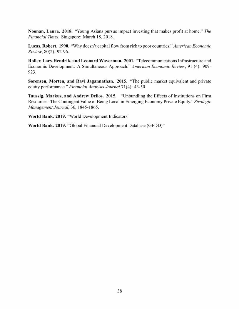
Noonan, Laura. 2018. “Young Asians pursue impact investing that makes profit at home.” TheFinancial Times. Singapore: March 18, 2018.

Lucas, Robert. 1990. “Why doesn’t capital flow from rich to poor countries,”American EconomicReview, 80(2): 92-96.

Roller, Lars-Hendrik, and LeonardWaverman. 2001. “Telecommunications Infrastructure andEconomic Development: A Simultaneous Approach.” American Economic Review, 91 (4): 909-923.

Sorensen, Morten, and Ravi Jagannathan. 2015. “The public market equivalent and privateequity performance.” Financial Analysts Journal 71(4): 43-50.

Taussig, Markus, and Andrew Delios. 2015. “Unbundling the Effects of Institutions on FirmResources: The Contingent Value of Being Local in Emerging Economy Private Equity.” StrategicManagement Journal, 36, 1845-1865.

World Bank. 2019. “World Development Indicators”

World Bank. 2019. “Global Financial Development Database (GFDD)”

38

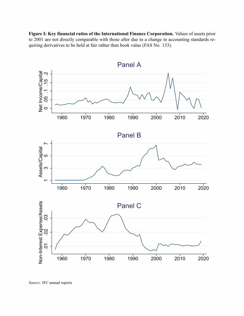
Figure I: Key financial ratios of the International Finance Corporation. Values of assets priorto 2001 are not directly comparable with those after due to a change in accounting standards re-quiring derivatives to be held at fair rather than book value (FAS No. 133).

0.0

5.1

.15

.2N

et In

com

e/C

apita

l

1960 1970 1980 1990 2000 2010 2020

Panel A

13

57

Asse

ts/C

apita

l

1960 1970 1980 1990 2000 2010 2020

Panel B

.01

.02

.03

Non

-Inte

rest

Exp

ense

/Ass

ets

1960 1970 1980 1990 2000 2010 2020

Panel C

Source: IFC annual reports

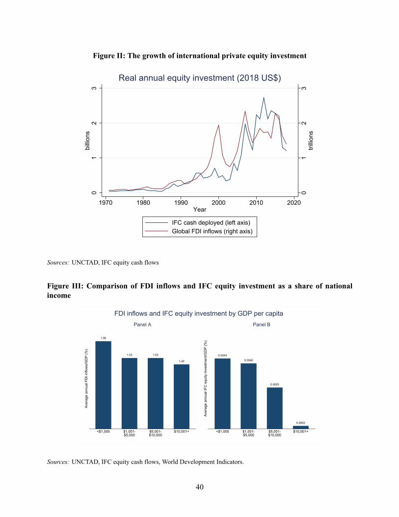
Figure II: The growth of international private equity investment

01

23

trillio

ns

01

23

billio

ns

1970 1980 1990 2000 2010 2020Year

IFC cash deployed (left axis)Global FDI inflows (right axis)

Real annual equity investment (2018 US$)

Sources: UNCTAD, IFC equity cash flows

Figure III: Comparison of FDI inflows and IFC equity investment as a share of nationalincome

1.90

1.53 1.53

1.40

Aver

age

annu

al F

DI i

nflo

ws/

GD

P (%

)

<$1,000 $1,001-$5,000

$5,001-$10,000

$10,001+

Panel A

0.0044

0.0040

0.0025

0.0002

Aver

age

annu

al IF

C e

quity

inve

stm

ent/G

DP

(%)

<$1,000 $1,001-$5,000

$5,001-$10,000

$10,001+

Panel B

FDI inflows and IFC equity investment by GDP per capita

Sources: UNCTAD, IFC equity cash flows, World Development Indicators.

40

Figure IV: Individual equity investment performance by decade

0.2

.4.6

.81

Kern

el d

ensi

ty

0 1 2 3+Investment-level PME vs. S&P 500

1961-1969 1970-1979 1980-19891990-1999 2000-2009 2010-2019

Panel A0

.2.4

.6.8

Kern

el d

ensi

ty

0 1 2 3+Investment-level TVPI

1961-1969 1970-1979 1980-19891990-1999 2000-2009 2010-2019

Panel B

Source: IFC equity cash flowsNote: For the graph, values above 3 were recorded as 3.

41

TABLE I: Geographic distribution of IFC equity investment compared to foreign direct invest-ment. This table presents IFC equity investment and global FDI flows by region. Advanced economiesare as classified by the IMF as of 2019. Advanced economies with IFC equity investments are, in de-scending order of real cash deployed: the Republic of Korea, Greece, Czech Republic, Slovak Republic,Latvia, Singapore, Estonia, Slovenia, Lithuania and Taiwan (China). Brazil; China, Russian Federation,Nigeria, India and Saudi Arabia are the largest FDI destinations in their regions. The United States;United Kingdom; and Hong Kong SAR (China) are the world’s three largest FDI destinations amongadvanced economies. The British Virgin Islands, Cayman Islands and United Arab Emirates are thethree largest Emerging Market and Developing Economies FDI destinations without IFC cash deployed.World region IFC projects are grouped under Emerging Market and Developing Economies. RegionalIFC projects are grouped under their region. FDI inflows from UNCTAD up to 2018. Values are 2018dollars, converted from nominal dollars using the US GDP deflator.

IFC equity investment since 1956 FDI inflows since 1970

Billions ($) Share of SUB-TOTAL

Trillions ($) Share of SUB-TOTAL Share of TOTAL IFC / FDI

A) Countries with IFC cash deployed

Emerging Market and Developing Economies 33.77 97.7% 11.33 85.9% 29.1% 0.30%

Latin America and the Caribbean 8.01 23.2% 3.45 26.2% 8.9% 0.23%

Brazil 2.23 6.50% 1.19 9.00% 3.10% 0.19%East Asia and the Pacific 6.28 18.20% 3.67 27.80% 9.40% 0.17%

China 3.22 9.30% 2.57 19.50% 6.60% 0.13%Europe and Central Asia 6.37 18.40% 2.02 15.30% 5.20% 0.32%

Russian Federation 1.85 5.40% 0.61 4.60% 1.60% 0.30%Sub-Saharan Africa 3.9 11.30% 0.7 5.30% 1.80% 0.56%

Nigeria 0.35 1.00% 0.15 1.10% 0.40% 0.24%South Asia 4.45 12.90% 0.67 5.10% 1.70% 0.66%

India 3.31 9.60% 0.56 4.30% 1.40% 0.59%Middle East and North Africa 3.22 9.30% 0.81 6.10% 2.10% 0.40%

Saudi Arabia 0.08 0.2% 0.31 2.3% 0.8% 0.03%World Region 1.54 4.5% - - - -

Advanced Economies 0.78 2.3% 1.87 14.1% 4.8% 0.04%

Korea, Rep. 0.30 0.9% 0.29 2.2% 2.2% 0.10%Greece 0.20 0.6% 0.08 0.6% 0.6% 0.25%Czech Republic 0.18 0.5% 0.17 1.3% 1.3% 0.11%

SUB-TOTAL 34.56 100.0% 13.19 100.0% 33.9% 0.26%

B) Countries without IFC cash deployed

Emerging Market and Developing Economies 1.89 4.9%

British Virgin Islands 0.84 2.2%Cayman Islands 0.59 1.5%United Arab Emirates 0.17 0.4%

Advanced Economies 23.86 61.3%

United States 7.02 18.0%United Kingdom 2.68 6.9%Hong Kong SAR (China) 1.68 4.3%

TOTAL 38.95 100.0% 0.09%42

TABLE II: IFC equity investment strategy described by a panel vector autoregression. Anobservation is a country year. IFC/GDP refers to IFC equity portfolio cash deployed as a share ofGDP in a given country year. FDI/GDP refers to FDI inflows as a share of GDP. WB/GDP refersthe value of board approved World Bank lending committments (through either the InternationalDevelopment Association and the International Bank for Reconstruction and Development) as ashare of GDP. Crises and sovereign debt restructuring are as reported by Leaven and Valencia(2020). Standard errors are clustered at the country level. ***p<0.01, ** p<0.05, * p<0.1

(1) (2) (3)

(IFC/GDP)x100 FDI/GDP WB/GDP

(IFC/GDP)x100 (t-1) 0.046* 0.056 0.006(0.027) (0.062) (0.010)

(IFC/GDP)x100 (t-2) 0.055* 0.008 0.005(0.032) (0.038) (0.006)

FDI/GDP (t-1) 0.005 -0.078 0.001(0.005) (0.691) (0.002)

FDI/GDP (t-2) 0.003 -0.098 0.000(0.003) (0.370) (0.001)

WB/GDP (t-1) 0.075 -0.418 0.005(0.103) (0.472) (0.143)

WB/GDP (t-2) -0.001 -0.317 0.101(0.031) (0.378) (0.093)

Banking Crisis (=1) -0.001 -0.006 0.003***(0.001) (0.010) (0.001)

Currency Crisis (=1) -0.001 -0.016 0.004***(0.001) (0.017) (0.001)

Sovereign Default (=1) -0.003* -0.018** -0.000(0.002) (0.008) (0.002)

Sovereign Debt Restructuring (=1) -0.002 -0.011 0.005**(0.002) (0.009) (0.002)

Observations 7,686 7,686 7,686

p-values of Chi-squared tests:H0: Coefficients on both lags of FDI/GDP = 0 in Column (1) 0.498H0: Coefficients on both lags of IFC/GDP = 0 in Column (2) 0.216H0: Coefficients on both lags of WB/GDP = 0 in Column (1) 0.584H0: Coefficients on both lags of IFC/GDP = 0 in Column (3) 0.715

43

TABLE III: Financial performance of the IFC private equity portfolio as of June 30, 2019.The publicmarket equivalent (PME) ismeasured followingKaplan and Schoar (2005) as the ratio ofcash in (disbursements) to cash out (client capital calls), where each series is discounted accordingto a public market index. The discount rate is given by the total return of the index, includingdividends and price appreciation. Cash flows and the index value are observed on the last date ofeach month. For investments with non-zero holding valuation, the fair value is treated as a positivecash flow in June 30, 2019, as if the investment is sold on that date. An investment is consideredfully realized if it has zero holding valuation.

Index Start DateFinancial performance of the portfolio of all equity invest-ments with vintage years including and since...

1961 1970 1980 1990 2000 2010

PME vs. MSCI Emerging Markets 1988 1.3 1.18 0.98PME vs. MSCI World 1970 1.21 1.26 1.23 1.12 0.78PME vs. S&P 500 1957 1.15 1.13 1.16 1.14 1.07 0.7

Total value to paid-in (TVPI) 1.71 1.70 1.69 1.61 1.47 1.15

Number of investments 2,509 2,429 2,304 2,053 1,433 803Share of investments fully realized 69.20% 68.20% 66.40% 62.50% 47.50% 25.80%

44

TABLE IV: Investment financial performance and investment size. Total cash deployed across2,509 companies is classifed into investment size quartiles by decade. Panel A reports the cutoffs for each quartile. Panel B reports the returns to a synthetic portfolio made up of only theinvestments in each quartile. For the PME vs. MSCI Emerging Markets, projects are included inthe calculation if they have vintage years after 1988, when the index began. For the PME vs. MSCIWorld, projects are included if they have vintage years on or after 1970. For the PME vs. S&P500, all projects are included.

Panel A) Investment size cutoffs by decade (nominal $ millions)

Time Period BottomQuartile

Median TopQuartile

Mean

1959-69 0.33 0.72 2.02 1.321970-79 0.35 0.88 2.00 1.851980-89 0.30 0.84 2.50 3.011990-99 0.60 2.22 6.09 5.282000-09 2.04 6.00 15.45 13.172010-19 4.00 10.00 21.76 19.49

Panel B) Portfolio performance by size quartile

Investment size TVPI PME vs.S&P 500

PME vs.MSCIWorld

PME vs.MSCIEmergingMarkets

1st quartile (smallest) 2.18 1.48 1.44 1.852nd quartile 1.83 1.16 1.2 1.263rd quartile 1.68 1.02 1.11 1.214th quartile (largest) 1.69 1.18 1.24 1.36

45

TABLE V: Investment financial performance and market size. The dependent variable is thePME vs. S&P500, winsorized at the 99th percentile. Independent variables are the population andGDP per capita of the country, on the year of the first cash flow associated with the investment.Panel A reports a linear regression with the constant not reported. Panel B reports the same re-gression, but with fixed effects for 22 subsectors that partition IFC’s four sectoral departments:Manufacturing, Agriculture and Services; Financial Institutions; Infrastructure; and Collective In-vestment Vehicles (funds). Panel C reports the same regression, excluding the five most recentvintage years, whose performance is disproportionately determined by mark to market valuations.Standard errors are clustered at the country-year. *** p<0.01, ** p<0.05, * p<0.1

(1) (2) (3) (4) (5) (6)

Quantile Regressions

OLS 0.1 0.25 0.5 0.75 0.9

PME PME PME PME PME PME

Panel A) Baseline specification

Ln(Population) 0.028 0.003 0.010 0.019** 0.023* 0.025(0.021) (0.005) (0.008) (0.009) (0.014) (0.026)

Ln(GDP per capita) 0.025 0.003 0.033** 0.050** 0.041 -0.068(0.044) (0.010) (0.013) (0.020) (0.029) (0.048)

R-squared (pseudo) 0.096 0.035 0.060 0.072 0.096 0.164Observations 2,069 2,069 2,069 2,069 2,069 2,069

Sample Full Full Full Full Full FullVintage year fixed effects Yes Yes Yes Yes Yes YesSector fixed effects No No No No No No

Panel B) Baseline specification with sector fixed effects

Ln(Population) 0.038* 0.004 0.010 0.016* 0.022 0.050**(0.021) (0.005) (0.007) (0.009) (0.016) (0.024)

Ln(GDP per capita) 0.033 0.004 0.019 0.055*** 0.053 0.045(0.044) (0.009) (0.012) (0.020) (0.037) (0.060)

R-squared (pseudo) 0.131 0.047 0.085 0.091 0.117 0.202Observations 2,069 2,069 2,069 2,069 2,069 2,069

Sample Full Full Full Full Full FullVintage year fixed effects Yes Yes Yes Yes Yes YesSector fixed effects Yes Yes Yes Yes Yes Yes

Panel C) Baseline specification with sector fixed effects, including only vintage years < 2015

Ln(Population) 0.036 0.002 0.005 0.017 0.023 0.076**(0.024) (0.006) (0.007) (0.011) (0.018) (0.039)

Ln(GDP per capita) 0.045 0.004 0.022 0.067*** 0.068* 0.050(0.050) (0.010) (0.013) (0.021) (0.038) (0.094)

R-squared (pseudo) 0.134 0.026 0.068 0.093 0.121 0.202Observations 1,837 1,837 1,837 1,837 1,837 1,837

Sample Pre-2015 Pre-2015 Pre-2015 Pre-2015 Pre-2015 Pre-2015Vintage year fixed effects Yes Yes Yes Yes Yes YesSector fixed effects Yes Yes Yes Yes Yes Yes

46

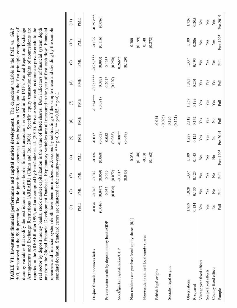
TABLEVI:Investmentfin

ancialperformance

andcapitalm

arketdevelopm

ent.

Thedependentv

ariableisthePM

Evs.S&

P500,winsorized

atthe99thpercentile.

Thede

jurefinancialopennessindexbegins

in1970,and

isthefirstprinciplecomponentof

dummyvariables

thatcodify

therestrictions

oncross-borderfinancialtransactions

reportedintheIM

F’sAnnualR

eportonExchange

ArrangementsandExchange

Restrictions

(AREA

ER)(Chinn

andIto,2008).

Specificequity

transactionrightsof

nonresidentsare

reportedintheAREA

ERafter1995,andarecompiledby

Fernándezet.al.(2015).P

rivatesectorcreditisdomestic

privatecredittothe

realsectorby

depositm

oney

banks;stockmarketcapitalizationisthevalueoflistedshares.Bothindicatorsoffinancialsystem

depth

arefrom

theGlobalFinancialDevelopmentD

atabase.

Explanatoryvariablesareallm

easuredintheyearoffirstcash

flow.Financial

opennessandfinancialsystem

depthhave

been

normalized

asZ-scoresby

subtractingoffthe

samplemeananddividing

bythesample

standarddeviation.Standarderrorsareclusteredatthecountry-year.***p<0.01,**p<0.05,*

p<0.1

(1)

(2)

(3)

(4)

(5)

(6)

(7)

(8)

(9)

(10)

(11)

PME

PME

PME

PME

PME

PME

PME

PME

PME

PME

PME

De-jurefinancialopennessindex

-0.034

-0.043

-0.042

-0.094

-0.037

-0.254***

-0.253***

-0.257***

-0.136

-0.253***

(0.046)

(0.047)

(0.059)

(0.068)

(0.062)

(0.081)

(0.082)

(0.093)

(0.116)

(0.086)

Privatesectorcreditby

depositm

oney

banks/GDP

-0.035

-0.049

-0.052

-0.201*

-0.463*

(0.034)

(0.072)

(0.088)

(0.107)

(0.250)

Stockmarketcapitalization/GDP

-0.081*

-0.108**

0.266**

(0.043)

(0.049)

(0.129)

Non-residentscanpurchaselocalequity

shares{0,1}

-0.038

0.300

(0.148)

(0.199)

Non-residentscanselllocalequity

shares

-0.101

0.148

(0.162)

(0.272)

Britishlegalorigins

-0.034

(0.095)

Socialistlegalorigins

0.126

(0.121)

Observations

1,859

1,828

1,337

1,109

1,227

2,112

1,859

1,828

1,337

1,109

1,726

R-squared

0.134

0.135

0.123

0.143

0.125

0.132

0.199

0.201

0.193

0.206

0.205

Vintage

yearfixed

effects

Yes

Yes

Yes

Yes

Yes

Yes

Yes

Yes

Yes

Yes

Yes

Sectorfixed

effects

Yes

Yes

Yes

Yes

Yes

Yes

Yes

Yes

Yes

Yes

Yes

Countryfixed

effects

No

No

No

No

No

No

Yes

Yes

Yes

Yes

Yes

Sample

Full

Full

Full

Post-1995

Pre-2015

Full

Full

Full

Full

Post-1995

Pre-2015

47

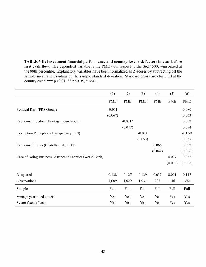
TABLE VII: Investment financial performance and country-level risk factors in year beforefirst cash flow. The dependent variable is the PME with respect to the S&P 500, winsorized atthe 99th percentile. Explanatory variables have been normalized as Z-scores by subtracting off thesample mean and dividing by the sample standard deviation. Standard errors are clustered at thecountry-year. *** p<0.01, ** p<0.05, * p<0.1

(1) (2) (3) (4) (5) (6)

PME PME PME PME PME PME

Political Risk (PRS Group) -0.011 0.080(0.067) (0.063)

Economic Freedom (Heritage Foundation) -0.081* 0.032(0.047) (0.074)

Corruption Perception (Transparency Int’l) -0.034 -0.059(0.053) (0.057)

Economic Fitness (Cristelli et al., 2017) 0.066 0.062(0.042) (0.066)

Ease of Doing Business Distance to Frontier (World Bank) 0.037 0.032(0.036) (0.088)

R-squared 0.138 0.127 0.139 0.037 0.091 0.117Observations 1,009 1,029 1,031 707 446 392

Sample Full Full Full Full Full Full

Vintage year fixed effects Yes Yes Yes Yes Yes YesSector fixed effects Yes Yes Yes Yes Yes Yes

48

TABLE VIII: Investment financial performance and macroeconomic variables recorded inthe year before the first cash flow. The dependent variable is the PME with respect to the S&P500, winsorized at the 99th percentile. All independent variables are changes between the year offirst cash flow and the previous year. Real GDP growth (in USD), inflation (change in LC GDPdeflator) and currency depreciation (change in USD/LC) are from the WDI. Central governmentdebt is from the International Financial Statistics. Sovereign rating is the (reverse) composite indexprovided by Oxford Economics based on the average of the sovereign ratings provided byMoody’s,S&P and Fitch, ranging from 1 to 20, where 20 is the worst possible credit rating. Higher valuesindicate higher credit risk. Regression constant is not reported. Standard errors are clustered at thecountry-year.*** p<0.01, ** p<0.05, * p<0.1

(1) (2) (3) (4) (5) (6) (7) (8)

PME PME PME PME PME PME PME PME

Real GDP growth rate 1.211 1.653* 1.966 0.444(0.969) (0.991) (1.203) (1.323)

Inflation rate 0.140 0.017 0.021 0.745(0.126) (0.483) (0.583) (0.618)

Currency depreciation rate 0.129 0.138 0.134 -0.749(0.128) (0.494) (0.602) (0.636)

Central government debt (% GDP) -0.001 -0.001 -0.001(0.001) (0.001) (0.003)

Sovereign rating index -0.000 0.026(0.018) (0.027)

R-squared 0.107 0.107 0.106 0.129 0.094 0.126 0.158 0.146Observations 2,065 2,066 2,105 1,668 1,336 2,062 1,641 1,073

Sample Full Full Full Full Full Full Full Full

Vintage year fixed effects Yes Yes Yes Yes Yes Yes Yes YesSector fixed effects Yes Yes Yes Yes Yes Yes Yes Yes

49

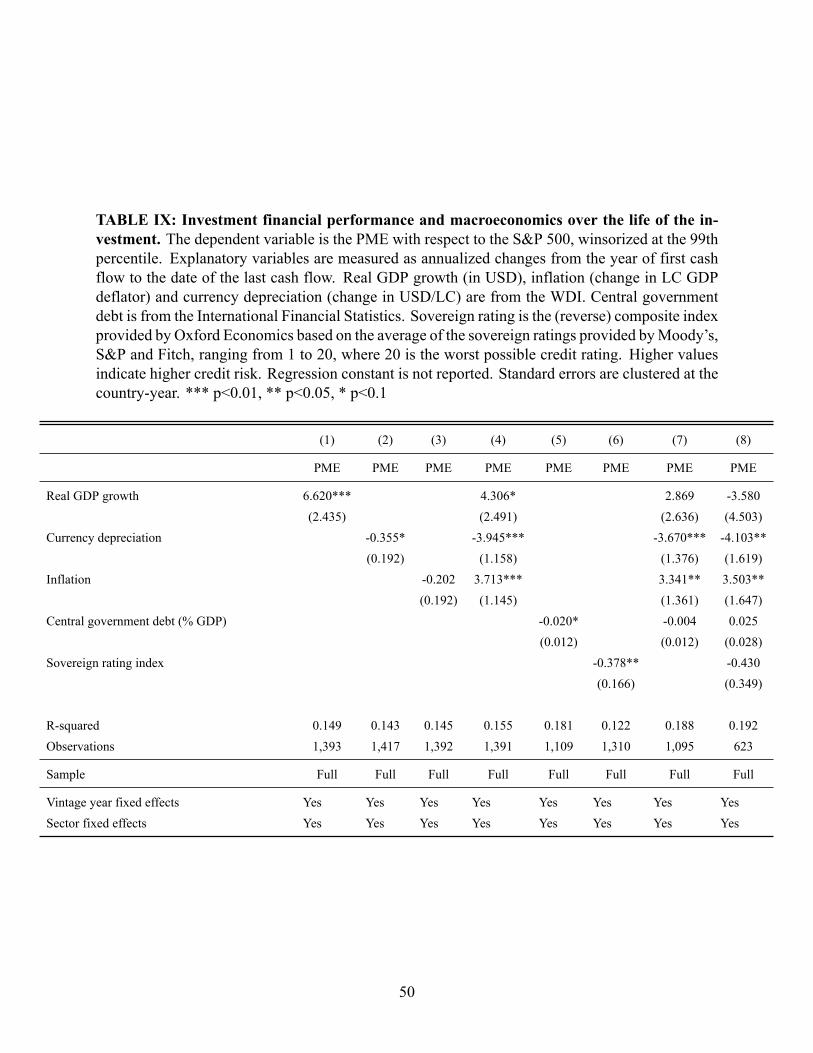
TABLE IX: Investment financial performance and macroeconomics over the life of the in-vestment. The dependent variable is the PME with respect to the S&P 500, winsorized at the 99thpercentile. Explanatory variables are measured as annualized changes from the year of first cashflow to the date of the last cash flow. Real GDP growth (in USD), inflation (change in LC GDPdeflator) and currency depreciation (change in USD/LC) are from the WDI. Central governmentdebt is from the International Financial Statistics. Sovereign rating is the (reverse) composite indexprovided by Oxford Economics based on the average of the sovereign ratings provided byMoody’s,S&P and Fitch, ranging from 1 to 20, where 20 is the worst possible credit rating. Higher valuesindicate higher credit risk. Regression constant is not reported. Standard errors are clustered at thecountry-year. *** p<0.01, ** p<0.05, * p<0.1

(1) (2) (3) (4) (5) (6) (7) (8)

PME PME PME PME PME PME PME PME

Real GDP growth 6.620*** 4.306* 2.869 -3.580(2.435) (2.491) (2.636) (4.503)

Currency depreciation -0.355* -3.945*** -3.670*** -4.103**(0.192) (1.158) (1.376) (1.619)

Inflation -0.202 3.713*** 3.341** 3.503**(0.192) (1.145) (1.361) (1.647)

Central government debt (% GDP) -0.020* -0.004 0.025(0.012) (0.012) (0.028)

Sovereign rating index -0.378** -0.430(0.166) (0.349)

R-squared 0.149 0.143 0.145 0.155 0.181 0.122 0.188 0.192Observations 1,393 1,417 1,392 1,391 1,109 1,310 1,095 623

Sample Full Full Full Full Full Full Full Full

Vintage year fixed effects Yes Yes Yes Yes Yes Yes Yes YesSector fixed effects Yes Yes Yes Yes Yes Yes Yes Yes

50

TABLEX: Investment financial performance and holding durationDuration is measured as thenumber of years between the first and last cash flow. Columns 3 and 4 include only investmentsthat have been realized, and have a current holding valuation equal to zero. Standard errors areclustered at the country-year. *** p<0.01, ** p<0.05, * p<0.1

(1) (2) (3) (4)

PME PME PME PME

Duration 0.040*** 0.045***(0.009) (0.011)

Duration X 1(Duration < 5) 0.090** 0.092**(0.038) (0.037)

Duration X 1(5 ≤ Duration < 10) 0.089*** 0.091***(0.020) (0.022)

Duration X 1(10 ≤ Duration) 0.046*** 0.050***(0.010) (0.011)

R-squared 0.120 0.124 0.124 0.127Observations 2,509 2,509 1,736 1,736

Sample Full Full Realized Realized

Vintage year fixed effects Yes Yes Yes YesSector fixed effects Yes Yes Yes Yes

51

APPENDIX A: Historical IFC Financial Statements and Ratios. Balance sheet and incomestatement values are as reported in the annual report, including revisions. Total assets prior to 1974do not include the undrawn portion of a loan from the International Bank for Reconstruction andDevelopment. Values of assets prior to 2001 are not directly comparable with those after due to achange in accounting standards requiring derivatives to be held at fair rather than book value (FASNo. 133) Return on equity is net income/total capital. Return on assets is net income/total assets.The leverage ratio is total assets/total capital. The expense ratio is non-interest expense/total assets.

Fiscal YearBalance Sheet Income Statement Financial Ratios

TotalCapital

Total Assets NetIncome

Non-InterestExpense

Return on Equity Return on Assets Leverage Expense

$ Mn $ Mn $ Mn $ Mn

1957 93.5 93.6 1.7 0.7 1.79% 1.79% 1.001 0.78%1958 97.3 97.4 2.4 1.1 2.42% 2.42% 1.001 1.18%1959 99.4 99.5 1.7 1.4 1.75% 1.75% 1.001 1.42%1960 104.3 104.5 2.1 1.7 1.99% 1.99% 1.002 1.63%1961 107.2 107.8 2.4 2.0 2.20% 2.19% 1.006 1.87%1962 109.8 111.6 2.6 2.0 2.40% 2.36% 1.016 1.77%1963 115.2 115.4 3.3 2.2 2.88% 2.87% 1.001 1.87%1964 119.3 119.4 2.9 2.5 2.44% 2.44% 1.001 2.06%1965 122.2 122.3 3.0 2.7 2.46% 2.46% 1.001 2.23%1966 128.2 128.4 4.4 3.1 3.40% 3.40% 1.001 2.38%1967 134.8 134.9 6.0 3.2 4.47% 4.47% 1.001 2.37%1968 142.9 143.2 6.2 3.5 4.37% 4.36% 1.002 2.46%1969 155.2 156.0 7.5 4.1 4.81% 4.78% 1.005 2.66%1970 165.8 184.1 10.3 5.4 6.18% 5.57% 1.111 2.91%1971 172.1 237.0 6.2 6.5 3.58% 2.60% 1.377 2.74%1972 179.7 264.7 8.0 7.1 4.43% 3.00% 1.473 2.67%1973 166.7 278.9 4.2 7.5 2.50% 1.49% 1.673 2.70%1974 172.5 355.5 5.9 9.2 3.44% 1.67% 2.060 2.58%1975 178.2 457.6 5.4 10.4 3.03% 1.18% 2.568 2.28%1976 186.7 523.7 7.7 11.4 4.12% 1.47% 2.805 2.18%1977 195.7 653.8 8.9 13.1 4.55% 1.36% 3.340 2.01%1978 243.8 720.8 12.5 16.2 5.13% 1.73% 2.957 2.24%1979 347.7 819.7 19.2 20.9 5.52% 2.34% 2.357 2.55%1980 446.4 907.8 20.7 26.5 4.63% 2.28% 2.034 2.92%1981 551.3 1,084.8 19.5 34.3 3.53% 1.80% 1.968 3.16%1982 678.1 1,233.4 21.6 39.3 3.18% 1.75% 1.819 3.18%1983 747.6 1,313.8 23.1 43.1 3.08% 1.75% 1.757 3.28%1984 774.3 1,389.9 26.3 45.0 3.40% 1.89% 1.795 3.24%1985 804.2 1,672.8 28.3 51.5 3.52% 1.69% 2.080 3.08%1986 885.6 2,236.4 25.4 60.2 2.87% 1.14% 2.525 2.69%1987 1,059.2 2,814.1 53.8 63.7 5.08% 1.91% 2.657 2.27%1988 1,288.5 3,427.0 100.6 71.6 7.80% 2.93% 2.660 2.09%52

Fiscal YearBalance Sheet Income Statement Financial Ratios

TotalCapital

Total Assets NetIncome

Non-InterestExpense

Return on Equity Return on Assets Leverage Expense

$ Mn $ Mn $ Mn $ Mn

1989 1,582.6 4,006.1 196.5 76.8 12.41% 4.90% 2.531 1.92%1990 1,864.1 5,606.3 157.0 105.9 8.42% 2.80% 3.008 1.89%1991 2,104.0 6,648.2 165.9 119.7 7.88% 2.49% 3.160 1.80%1992 2,389.3 8,132.7 180.2 139.7 7.54% 2.22% 3.404 1.72%1993 2,702.4 8,913.4 141.7 163.2 5.25% 1.59% 3.298 1.83%1994 3,198.1 14,722.8 258.2 175.2 8.07% 1.75% 4.604 1.19%1995 3,602.8 18,227.6 188.0 171.0 5.22% 1.03% 5.059 0.94%1996 4,158.2 22,640.2 345.8 185.4 8.32% 1.53% 5.445 0.82%1997 4,736.9 28,974.7 431.9 204.5 9.12% 1.49% 6.117 0.71%1998 5,084.3 31,620.7 245.8 218.0 4.83% 0.78% 6.219 0.69%1999 5,344.2 33,456.2 249.3 258.0 4.66% 0.75% 6.260 0.77%2000 5,733.0 38,719.0 380.0 265.0 6.63% 0.98% 6.754 0.68%2001 6,095.0 26,170.0 345.0 304.0 5.66% 1.32% 4.294 1.16%2002 6,304.0 27,739.0 215.0 327.0 3.41% 0.78% 4.400 1.18%2003 6,789.0 31,543.0 487.0 332.0 7.17% 1.54% 4.646 1.05%2004 7,782.0 32,361.0 993.0 360.0 12.76% 3.07% 4.158 1.11%2005 9,798.0 39,560.0 2,015.0 403.0 20.57% 5.09% 4.038 1.02%2006 11,076.0 38,420.0 1,264.0 436.0 11.41% 3.29% 3.469 1.13%2007 14,017.0 40,599.0 2,490.0 482.0 17.76% 6.13% 2.896 1.19%2008 18,261.0 49,471.0 1,547.0 549.0 8.47% 3.13% 2.709 1.11%2009 16,122.0 51,483.0 -151.0 582.0 -0.94% -0.29% 3.193 1.13%2010 18,359.0 61,075.0 1,746.0 664.0 9.51% 2.86% 3.327 1.09%2011 20,279.0 68,490.0 1,579.0 700.0 7.79% 2.31% 3.377 1.02%2012 20,580.0 75,761.0 1,328.0 798.0 6.45% 1.75% 3.681 1.05%2013 22,275.0 77,525.0 1,018.0 845.0 4.57% 1.31% 3.480 1.09%2014 23,990.0 84,130.0 1,483.0 888.0 6.18% 1.76% 3.507 1.06%2015 24,426.0 87,548.0 445.0 901.0 1.82% 0.51% 3.584 1.03%2016 22,766.0 90,434.0 -33.0 933.0 -0.14% -0.04% 3.972 1.03%2017 25,053.0 92,254.0 1,418.0 962.0 5.66% 1.54% 3.682 1.04%2018 26,136.0 94,272.0 1,280.0 1,029.0 4.90% 1.36% 3.607 1.09%2019 27,606.0 99,257.0 93.0 1,355.0 0.34% 0.09% 3.595 1.37%

53

APPENDIX B: Equity investments by region and sector. Regions follow theWorld Bank Groupregional classifications as of 2019. Collective investment vehicles are private equity fundsmanagedby an institution other than IFC.

1961-69 1970-79 1980-89 1990-99 2000-09 2010-19 TOTAL

Panel A) Count of investments by region

Latin America and Caribbean 34 33 71 143 119 158 558East Asia and Pacific 7 29 53 97 122 154 462Sub-Saharan Africa 13 20 58 117 95 149 452South Asia 11 7 27 81 106 147 379Europe and Central Asia 5 15 13 123 118 77 351Middle East and North Africa 6 16 21 51 44 65 203World 4 5 8 8 26 53 104TOTAL 80 125 251 620 630 803 2,509

Panel B) Count of investments by sector

Finance and Insurance 22 20 40 133 222 193 630Collective Investment Vehicles - 2 26 136 137 231 532Oil, Gas and Mining 2 6 28 40 44 43 163Industrial and Consumer Products 8 7 32 31 15 16 109Chemicals 8 8 24 30 23 15 108Food and Beverages 4 4 22 37 14 17 98Electric Power 1 - - 26 11 58 96Nonmetallic Mineral Product Manufacturing 8 18 14 28 12 8 88Agriculture and Forestry 2 6 19 13 16 24 80Transportation and Warehousing - 2 6 23 16 33 80Textiles, Apparel and Leather 10 19 10 26 3 2 70Information 1 - 1 23 20 23 68Accommodation and Tourism Services 3 11 10 23 9 7 63Professional, Scientific and Technical Services - - 3 5 30 24 62Health Care - - - 9 15 29 53Pulp and Paper 5 8 6 13 7 4 43Primary Metals 6 10 7 10 4 1 38Utilities - - - 1 10 20 31Construction and Real Estate - - - 4 4 19 27Education Services - - 1 - 7 19 27Wholesale and Retail Trade - - - 5 7 15 27Plastics and Rubber - 4 2 4 4 2 16TOTAL 80 125 251 620 630 803 2,509

54

APPENDIX C: Equity investment financial performance in emerging market and developingeconomies. In the weighted average, each investment is weighted by the share of cumulative contri-butions in that that vintage year. Before calculation of averages, variables have been winsorized at the99th percentile, for consistency with the sample used in the regressions. Realized investments are thosewith zero holding valuation as of June 30, 2019.

Vintage Years Investments Realized Investments Duration**PME S&P 500 TVPI

Average Median WeightedAverage

Average Median WeightedAverage

1961-69 80 100.0% 17.4 1.44 1.02 1.35 3.18 1.84 2.751970-79 125 100.0% 14.0 0.90 0.51 0.94 3.22 1.37 3.511980-89 251 98.8% 11.5 0.98 0.45 1.17 2.90 1.21 3.301990-99 620 97.3% 9.3 1.34 0.65 1.39 2.47 1.19 2.542000-09 630 75.1% 8.2 1.60 0.87 1.84 2.32 1.26 2.592010-19 803 25.8% 4.5 0.81 0.74 0.84 1.23 1.00 1.25

ALL 2,509 69.1% 8.2 1.18 0.72 1.26 2.14 1.13 2.56

**Duration is defined as the average years between first and final cash flow or positive valuation

55

APP

ENDIX

D:Q

uantile

regressionsw

ithcapitalm

arketopennessa

nddevelopm

ent.ThedependentvariableisthePM

Evs.S

&P

500,winsorized

atthe99thpercentile.

Thede

jurefinancialopennessindexbegins

in1970,and

isthefirstprinciplecomponentof

dummyvariables

thatcodify

therestrictions

oncross-borderfinancialtransactions

reportedintheIM

F’sAnnualR

eportonExchange

ArrangementsandExchange

Restrictions

(AREA

ER)(Chinn

andIto,2008).Privatesectorcreditisdomestic

privatecredittothereal

sectorby

depositm

oney

banksfromtheGlobalFinancialDevelopmentD

atabase.Explanatoryvariablesareallm

easuredintheyearof

firstcashflow.F

inancialopennessandfinancialsystem

depthhave

been

normalized

asZ-scoresby

subtractingoffthe

samplemeanand

dividing

bythesamplestandarddeviation.Standarderrorsareclusteredatthecountry-year.***p<0.01,**p<0.05,*

p<0.1

(1)

(2)

(3)

(4)

(5)

(6)

(7)

(8)

(9)

(10)

Quantile

Regressions

0.1

0.25

0.5

0.75

0.9

0.1

0.25

0.5

0.75

0.9

VARIABLE

SPM

EPM

EPM

EPM

EPM

EPM

EPM

EPM

EPM

EPM

E

De-jurefinancial

-0.007

-0.044*

-0.069*

-0.161**

-0.371

opennessindex

(0.018)

(0.023)

(0.037)

(0.072)

(0.323)

Privatesectorcredit

0.001

0.014

0.012

-0.440**

-0.921**

bydepositm

oney

banks/GDP

(0.013)

(0.010)

(0.012)

(0.188)

(0.396)

Observations

1,859

1,859

1,859

1,859

1,859

2,058

2,058

2,058

2,058

2,058

Pseudo-R2

0.0503

0.0787

0.0712

0.0851

0.181

0.0525

0.0774

0.0660

0.0796

0.180

Sectorfixed

effects

Yes

Yes

Yes

Yes

Yes

Yes

Yes

Yes

Yes

Yes

Countryfixed

effects

Yes

Yes

Yes

Yes

Yes

Yes

Yes

Yes

Yes

Yes

Sample

Full

Full

Full

Full

Full

Full

Full

Full

Full

Full

56