Chapter 2

LONG-TERM CHANGES

M. Van Roozendael and G. Vaughan

Contributing Authors A. Engel, S. Godin, H. Jéiger, E. Kyro, B. Nat(jokat, C. Schiller, A. Weiss and R. Zander

HIGHLIGHTS

This section summarises the main scientific highlights arising from recent research activities in Europe on the issue of the long-term variability and change of stratospheric composition and meteorology. The bullet list below is meant to provide an overview of the European contribution to the subject. More complete and detailed scientific highlights including results from non-European researchers can be found in the recent WMO Scientific Assessment of Ozone Depletion: 1998, and SPARC Ozone and Water Vapour Assessments [Harris et al., 1998; Kley et al., 2000].

Ozone

• High quality long-term Dobson records in Europe show that total ozone declined after 1980 during all seasons, but especially in the January-April period. Recent measurements show that northern hemisphere total ozone has increased slightly in the last few years, although values are still below pre-1975 Ievels. The ozone hole in Antarctica continues unabated.

• The determination of ozone trends on the global scale relies on satellite measurements validated by ground-based observations. A European contribution to ozone monitoring from space became available in July 1995 with the Global Ozone Monitoring Experiment (GOME) onboard the ERS-2 platform, partly filling the gap from late 1994 to 1996 in the TOMS data record. The combined TOMS (N7, M3 and EP) and GOME satellite data set allows the Iatitudinal distribution of the 0 3 trends over the period 1979-2000 to be documented. These are Iargest for high latitudes in winter and overall statistically insignificant in the tropics. Current differences of the order of 5-15 DU between GOME, TOMS and ground-based total ozone measurements still need to be resolved to allow reliable assessment of changes in trend after 1995 in comparison to the pre-Pinatubo trend.

• Altitude resolved 0 3 trend analysis based on satellite and ozone sondes observations show the largest downward trend (approximately -7% per decade) arising in the upper stratosphere around 40 km altitude and in the lowermost stratosphere around 16 km. Recent re-evaluation of ground-based Umkehr observations available since the beginning of the sixties confirm the trend reported for the upper stratosphere. In the lowermost stratosphere, the derived trends are sensitive to the period chosen for analysis, and decrease substantially when the most recent years are included.

29

Stratospheric composition

• The total amount of organic chlorine (CCly) contained in long- and shorter-lived chlorocarbons reached maximum values of 3.6±0.1 ppbv between 1993 and 1994 and is beginning to decrease slowly in the troposphere mainly due to reduced emissions of methyl chloroform (CH3CC13).

• The loading of inorganic chlorine in the stratosphere, monitored since 1977 at the Jungfraujoch (Switzerland), reached a maximum around 1997, consistent with the reduction in emissions of important organic chlorine species achieved by international regulations (Montreal Protocol and its Amendments and Adjustments).

• Evaluations of the bromine budget in the stratosphere by two different methods provide evidence that stratospheric inorganic bromine has increased by about 25% during the decade 1987-1996. This increase consistently follows the measured trend in tropospheric source gases, which is primarily due to the increase in atmospheric halons H-1211, H-1301, H-2402 and H-1201. Continued increase of halons over the next few years could cause the abundance of equivalent chlorine to decline more slowly than predicted.

• A significant increase in the stratospheric water vapour concentration has been identified over recent decades. The European measurement record of H20, available since the 1990s, and that of other hydrogen species will become sufficiently large within the next few years to follow the current changes.

• The column abundance of CH_., monitored at the Jungfraujoch since 1950, has increased by 35% over the last fifty years but with a declining rate of growth during the last few years, in line with findings from in situ surface measurements of CH4 .

• An upward trend in NO2 column of about 5% per decade has been identified at the Jungfraujoch (Switzerland) during the last two decades. This increase, which is similar to the trend recently rep011ed at Lauder (New Zealand), is about twice the trend in tropospheric N20, the principal source of stratospheric NO 2 • Recent 2-D mode! calculations indicate that the difference could be explained by a long-term change in the NOJNOY pai1itioning due to an overall effective decrease of about 20% of the stratospheric aerosol loading between 1980 and 1998 related to the El Chichon and Mt Pinatubo volcanic eruptions.

• The two most recent major volcanic eruptions, El Chichon (1982) and Mt Pinatubo ( 1991) temporarily increased sulphate aerosol abundances by more than an order of magnitude. On the other band, backscatter lidar observations of stratospheric sulphate aerosol at Garmisch­Partenkirchen (Germany) show no clear trend from 1976-2000, indicating that any anthropogenic contribution must be smaller than thought in the previous EC report.

Temperature and dynamics

• Trends in stratospheric temperatures between 100 and 30 mb, derived from northern hemisphere radio sonde analyses available since 1965, are negative at all latitudes being greatest in the subtropics and polar regions around 50 mb, where they exceed ---0.7 K per decade. Calculated temperature trends strongly depend on the beginning and end dates considered for the analysis, especially in the highly variable winter stratosphere. For the

30

North Pole, Freie Universitiit Berlin (FUB) analyses at 30 mb from 1955-2000 show no significant trend for the whole period in March, but a strong cooling (-6 K per decade) since 1979. The same data set for July (when the inter-annual variability is much Jess) exhibit a significant overall cooling of 0.6 K per decade from 1955-2000 and 1.3 K per decade since 1979.

• Processes driving the natural variability of the northern hemisphere stratosphere are now better understood. In particular, the role of the Quasi-Biennial Oscillation (QBO) in stabilising the polar vortex during its westerly phases and in disturbing it during its easterly phases has been elucidated. Moreover the role played by the solar cycle in modulating this connection has been further established. It has also been shown that warm events of the El Nino/Southern Oscillation (ENSO) often result in major mid-winter warmings, while strong volcanic eruptions like Mt Pinatubo (1991) result in a warming of the tropical stratosphere.

• New evidence has been found that the frequency of events mixing subtropical ozone-poor air into the mid-latitude stratosphere may have increased over the past twenty years, possibly explaining some of the observed ozone changes in northern mid-latitude regions.

• Significant progress has been achieved in characterising the polar vortex climatology, again based on ECMWF meteorological analyses covering the period 1979-2000. Results indicate that the polar vortices of the 1990s have been stronger and of longer duration than those in the 1980s, in accordance with the reported long-term cooling of the polar stratosphere.

• The North Atlantic Oscillation (NAO) and Arctic Oscillation (AO) are important components of long-period variability in the atmosphere, with the AO in particular being closely linked to the strength of the polar vortex. Recent GCM model experiments emphasise that a correct representation of the AO/NAO mode of variability is important to correctly represent the atmospheric response to stratospheric aerosol, stratospheric ozone loss, changes in solar activity, and increased greenhouse gas forcing.

2.1 INTRODUCTION

This chapter is concerned with two issues: changes in the abundance of trace species and aerosols, and long-term changes in meteorological conditions in the stratosphere. Both these factors impact on ozone, since its distribution results from a balance between chemistry and transport. In the extra-tropical lower stratosphere in particular, where there appear to be significant ozone trends [Harris et al., 1998], the ozone concentration is very sensitive to changes in circulation - both in the wave driven meridional circulation of the main stratosphere (the Brewer-Dobson circulation) and the isentropic mixing across the tropopause driven by synoptic scale dynamics in the troposphere. A thorough understanding of such changes is needed if the anthropogenic component of observed ozone changes is to be identified. In this chapter we present an update on the changes observed in stratospheric composition, temperature and circulation since the 1950s together with new work made possible by the ECMWF ERA-15 re-analyses. Together, they provide the backdrop against which changes in ozone must be interpreted. They also allow the dynamical changes themselves to be examined for trends (possibly linked to anthropogenically-forced climate change) and low-frequcncy oscillations in the atmosphere and oceans, for example the solar cycle, QBO and AO.

31

During recent decades, concern about the erosion of the ozone layer has led to reductions in the anthropogenic emissions of several halogen bearing source gases with large Ozone Depletion Potentials (ODPs), as identified in the Montreal Protocol ( 1987) and its subsequent Amendments and Adjustments. This has had a notable influence on the chlorine loading of the stratosphere, which has been the primary cause of ozone layer depletion at the spring poles. European contributions to long-term change investigations in the stratosphere have resulted mainly from involvements in the Network for the Detection of Stratospheric Change (NDSC) and from the investigation of individual data sets gathered during stratospheric balloon flights. This chapter summarises the salient results of these investigations.

Since the last EC assessment in 1996, the stratosphere bas experienced a period of very low aerosol abondance; the perturbation due to Mt Pinatubo has decayed away and aerosol loadings are now at their lowest level recorded since the late 1970s. In addition, the period has been one of very marked inter-annual variability at high latitudes, with two very warm winters ( 1997 /98 and 1998/99) followed by one of the coldest on record (1999/2000). Such inter-an nuai variability means that very long records (or very large changes) are needed before statistically significant trends in temperature, circulation and chemical composition can be discerned from noise; the same is necessarily true for ozone.

2.2 CHANGES IN OZONE

This section considers only the observational evidence for ozone changes. Interpretation and trend analysis are presented in Chapter 4. For a fuller description of the methods used to measure ozone and of the observed trends, see Staehlin et al. [2001].

2.2.1 Ground-based measurements of total ozone

The first observational evidence of long-term changes to the ozone layer came from the Dobson spectrophotometer measurements at Halley Bay, Antarctica (76°S). The drastic reduction in total ozone during spring [Farman et al., 1985] ale11ed the scientific community and the general public to the existence of the ozone hole and set in train an extensive research and monitoring effort to understand the changes. The monthly mean total ozone at Halley Bay for each October from 1955-2000 is shown in Figure 2.1, clearly demonstrating the development of the ozone hole after 1975 with a levelling off of the October mean values in recent years. Ozone sonde measurements from Antarctica in the 1990s [Hofmann et al., l 997] show almost complete destruction of the ozone layer between 14 and 18 km by mid-October, with significant depletion between 12 and 22 km.

Away from Antarctica the changes in total ozone are smaller, and are marked by considerable natural variability. The longest total ozone record in existence is that for Arosa, Switzerland [Staehelin et al., 1998]. This is shown in Figure 2.2 for three separate four-mon th periods. In each case no systematic change in ozone can be discerned from the noise before about 1980. Since then, total ozone has declined at ail times of the year, with the greatest decrease (~30 DU) in the January-April period. In the last few years, total ozone has increased a little, although values remain below the pre-1975 mean.

Confirmation that the decline in total ozone in northern mid-latitudes occun-ed at ail longitudes, and was not peculiar to the European sector, is provided by Figure 2 .3. This shows the deviation of total ozone in winter from the long-term pre-1976 average for three longitude

32

Mean October ozone at Halley

450

400

350

--"' :!: C 300 :::::1

C 0

"' 250 ..Q

8 0 ._. 0

Q) 200 C ~ 0

N 0 (tj 150 ..... 0 1-

100

50

0 1950 1960 1970 1980 1990 2000 2010

Year

Figure 2.1 October mean total ozane measured by Dobson spectrophotometer at Halley Bay (76"S) from 1955 ta 2000. [Updatedfrom Farman et al., 1985 and Jones and Shanklin, 1995].

sectors; it is based on a composite of quality controlled ground-based observations and TOMS satellite measurements [Bojkov et al., 1998, 2000]. A similar picture to Figure 2.2 is found at all longitudes: a decline of ~8% in the 1980s to a minimum in 1992, followed by a slight increase in the 1990s.

Investigation of trends in total ozone and future identification of the recovery of the ozone layer require high quality and consistent long-term total ozone data from ground-based networks. For the Dobson part of the total ozone monitoring network in Europe, a Regional Dobson Calibration Center (RDCC) has been established and started to fonction in 1999. The RDCC is a joint operation by the Meteorological Observatory at Hohenpeissenberg (Germany)

33

::> 0

::> 0

::> 0

400

350

300

370

320

JFMA

V

MJJA

\ SONO

y 270._____._ ___ __._ ___ _._ ___ __,_ ___ __. ___ ---"'-----'------'

1930 1940 1950 1960 1970 1980 1990 2000

Year

Figure 2.2 Total o-::,one measured by Dobson spectrophotometer at Arasa, Swit-::,er/and, from 1926 to the present [updated from Staelzlin et al., 1998}. Data have been ai•eraged overfour-monthly intervals for each year.

and the Solar and Ozone Observatory at Hradec Kralove (Czech Republic). lts activities are linked with the GAW program of WMO and with the World Dobson Calibration Center, at NOAA-CMDL, Boulder, Colorado.

2.2.2 Satellite measurements of total ozone

Ground-based measurements of total ozone are relatively scarce outs ide northem mid-latitudes, and to extend Figure 2.3 to other latitude zones we must rely on satellite measurements. Regular total ozone measurements from satellites began in October 1978 with the Nimbus 7 TOMS (N7), which operated until 1993 [Heath et al., 1975; McPeters et al., 1996]. The TOMS series has been continued by instruments on the satellites METEOR-3 (M3, 1991-4), ADEOS ( 1996/97) and Earth Probe (EP, 1996 to the present). This frequent change of instrument in the 1990s (together with a data gap between November 1994 and June 1996) introduces some uncertainty into long-term changes derived from TOMS. A European contribution to ozone monitoring has become available in recent years from the GOME on ERS-2 [Bun-ows et al., 1999]. This has operated since July 1995, parti y filling the gap in the TOMS data record.

34

5

DJFM 0

I \

-5 .•.

~ 0

:<( -10 : .' ' ............ N. America

1 • 1

1 1 1 1

-15 Europe ,,

- - - - - Siberia -20

1975 79 83 87 91 95 99

Year

Figure 2.3 Area-averaged (45-65°N) total ozane departures (in %) from the long-term pre-1976 averages for December-March 1979-2000. The 2a error for each point is less than 6%. [Bojkov et al., 1998, 2000].

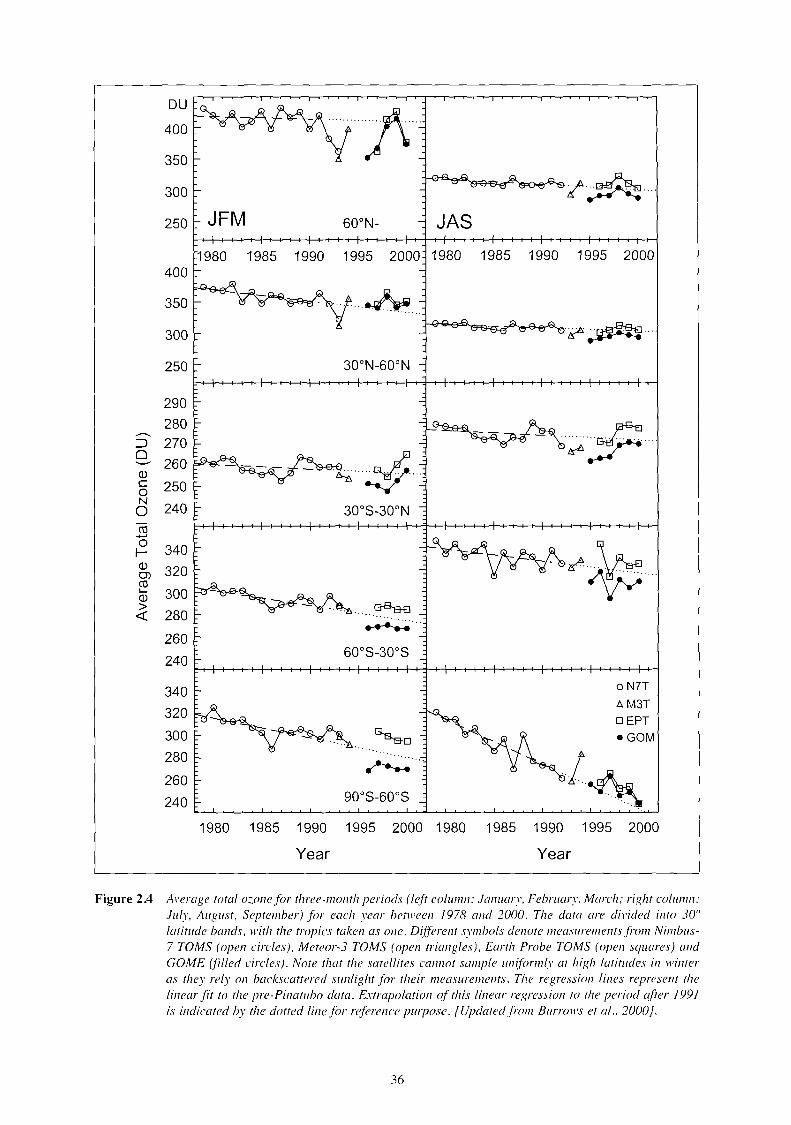
The satellite measurements are summarised in Figure 2.4. This shows the average total ozone over 30° latitude bands in winter and summer for the period 1979-2000 derived from the N7, M3 and EP TOMS instruments; also shown are corresponding GOME measurements beginning in 1995. None of the satellites can measure in the dark, so the values shown for high latitudes in winter are not as reliable as for the other panels. The TOMS data show an overall decline in ozone at all latitudes in both seasons. In the tropics the overall trend is small ( <0 .2 DU yr 1) and statistically insignificant since there is considerable decadal scale variability. Little overall trend is evident in the northem hemisphere summer, but in the winter months a steady decline is clear in mid-latitudes (about 2 DU yr 1

) and a very obvious change is seen at high latitudes around the time of the Mt Pinatubo eruption in 1991, with recovery to the long-term trend in 1998 and 1999. In Southern mid-latitudes the decline is marked in both seasons (at 1.0-1.5 DU yr 1) and not surprisingly very obvious at high latitudes in JAS. Minimum total ozone values below 100 DU have been measured in the ozone hole in the 1990s, while its maximum area (defined as that within the 220 DU contour) continues to increase [WMO, 1999].

The data gap in the TOMS data record between 1994 and 1996 has led to some difficulties in assessing the continuation of the observed long-term trend after 1994. According to the most recent WMO assessment [WMO, 1999 Figure 4.12], the average total ozone between 60°N and 60°S from N7 and EP TOMS (after removing variability due to season, solar cycle, and QBO) show an increase from 1994 to 1998, while Dobson measurements similarly filtered showed no

35

DU

J\ 400

350

300 ,t-~ --- .....

250 JFM 60°N- JAS

1980 1985 1990 1995 2000 1980 1985 1990 1995 2000 400

350 ··---~---

300 -?~---·

250 30°N-60°N

290 280 ~~::f! -----:::> 270

0 260

¾~ Q) C 250 0 N

240 0 30°S-30°N CU ...... 0 340 f-Q) 320 ~~·~ 0) ······· CU ,_

300 Q)

> G-8.s-Ei <( 280 ~--.

260

240 60°S-30°S

340 oN?T

320 b.M3T DEPT

300 ~ •GOM

280 ....._ l~ 260

240 90°s-60°s

1980 1985 1990 1995 2000 1980 1985 1990 1995 2000

Year Year

Figure 2.4 A1·erage total o-::.onefor three-month periods (left co/umn: January, February, March; right column: lu/y, August, September) for each year befl\'een 1978 and 2000. The data are di1·ided into 30" latitude bands, with the tropics taken as one. Dijferent symbols denote measurementsfrom Nimbus-7 TOMS (open circ/es), Meteor-3 TOMS (open triangles), Earth Probe TOMS (open squares) and GOME (fïl/ed circ/es). Note that the satellites cannot sample uniformly at high latitudes in winter as they rely on backscattered sunlight for their 111easure111ents. The regression fines represent the linear fit to the pre-Pinatubo data. Extrapolation of this linear regression to the period after 1991 is indicated by the dotfecl fine for reference purpose. [Updated fmm B111-r011•s et al., 2000].

36

change. Nevertheless, both data sets indicate that the downward trend prior to Pinatubo has not continued. In order to determine whether such changes are real, the issue of data quality has to be addressed.

From Figure 2.4 it is apparent that systematic deviations between the GOME V2.7 and TOMS V7 data exist. Comparison of GOME data with 76 NH Dobson stations showed that deviations are dependent on season. During spring a positive bias of GOME of about 1-2% is observed, which changes to about -3% in autumn [update from Burrows et al., 2000]; however, the average difference over four years is less than 0.5%. A similar seasonal pattern (shifted by half a year) is observed in the southern hemisphere [Bodeker et al., 2001]. EP TOMS total ozone data has a positive bias of about 1.5% in the northern hemisphere in all seasons [Burrows et al., 2000]. There is an apparent north-south asymmetry in the differences between EP TOMS and Dobson data [Lambert et al., 1999]. At 50°N the bias is about 6 DU on average, while at 50°S this bias increases to about 12 DU [Bodeker et al., 2001]. B y using Dobson data as a transfer standard, it was estimated that EP TOMS measures between 2 and 6 DU more than Nimbus 7 TOMS, depending on the latitude [Bodeker et al., 2001].

At least another decade of global satellite measurements is needed to confirm any changes in the long-term ozone trend, taking into account instrumental issues and other uncertainties as discussed in more detail in Chapter 4.

2.23 Changes in the ozone vertical profile

A detailed assessment of changes in ozone vertical profiles has been published by SPARC [Harris et al., 1998]. This assessment concluded that only four measurement techniques have produced records long enough to assess long-term changes: the satellite instruments SAGE ( 1 and 2) and SBUV, balloon-borne ozone sondes and the ground-based Umkehr method (which uses zenith-sky observations from the Dobson spectrophotometer at twilight). Below 20 km, ozone sondes alone were considered sufficiently accurate to derive changes, whereas from 20-50 km Umkehr and satellite data could also be used. Harris et al. [ 1998] concluded that, between 1980 and 1996, ozone losses were statistically significant at all altitudes between 12 and 50 km, and that there were two regions of maximum decrease: the upper stratosphere around 40 km and the lowermost stratosphere around 16 km. In both these regions a change of approximately -7% per decade in ozone concentration has been observed, separated by a layer in the mid-stratosphere (~25-35km) where the decrease was less than 3% per decade.

A recent European project called REVUE (Reconstruction of Vertical ozone distribution from Umkehr Estimates) has re-evaluated the long-term global Umkehr record, which goes back to the beginning of the sixties for some stations [Godin et al., 2000]. Using an improved Umkehr algorithm and a global aerosol climatology, a homogeneous data set of ozone vertical profiles was derived for 14 Umkehr stations. This data set showed improved agreement with satellite and ozone sonde data, especially in the lower stratosphere. Results are shown for European mid-latitude stations (Belsk, Observatoire de Haute Provence and Arosa) in Figure 2.5, as linear trends over two periods: 1978-1997 and 1978-1999. Also shown on this diagram are the corresponding trends derived from Payerne ozone sondes. The Umkehr inversion algorithm reports ozone values in Umkehr layers. These layers are approximately 5 km thick and are centered at the layer number times 5 km in height. Also shown on this diagram are the corresponding trends derived from ozone sondes. The Umkehr shows a consistent trend of -5% per decade in the upper stratosphere (layers 7-8) but a much smaller negative trend than

37

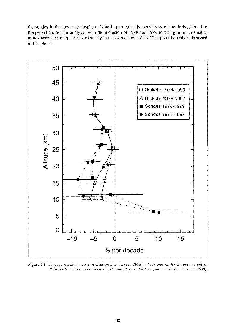
the sondes in the lower stratosphere. Note in particular the sensitivity of the derived trend to the period chosen for analysis, with the inclusion of 1998 and 1999 resulting in much smaller trends near the tropopause, particularly in the ozone sonde data. This point is further discussed in Chapter 4.

50

45

40

35

..- 30 E ~ ..._.. (]) 25

"'O :J

-t-1

-t-1

<( 20

15

10

5

0 -10 -5 0 5

□ Umkehr 1978-1999

.6. Umkehr 1978-1997

■ Sondes 1978-1999

• Sondes 1978-1997

.......... -.....

10 15

% perdecade

Figure 2.5 Average trends in ozane vertical profïles between 1978 and the present, for European stations: Belsk, OHP and Arasa in the case of Umkehr, Payeme for the ozone sondes. [Godin et al., 2000).

38

2.3 LONG-TERM CHANGES IN HALOGEN SPECIES

2.3.1 Chlorine species

As noted in Section 2.1, the emissions into the atmosphere of chlorine-containing chemicals with large ODPs (primarily all CFCs) have been reduced substantially in recent years. Chlorine source gases and resulting reactive chlorine species have been measured regularly both from the ground and from balloons by remote sensing and in situ techniques. However, only a few of these data sets have sufficient temporal coverage to allow a determination of long-term changes.

Surface measurements of the long- and shorter-lived halogenated sources gases contributing to the total organic chlorine loading of the atmosphere (CCly) have been provided since the late 1970s by two major global ground-based in situ networks: the ALE/GAGE/AGAGE network [Prinn et al., 1998] and the NOAA/CMDL network [Elkins et al., 2000]. The total CCly is defined as the sum of the chlorine atoms bound in all organic chlorine-bearing gases released to the atmosphere. As none of the monitoring networks measures all species making up CCly, it is in practice evaluated from available measurements of the dominant Cl-bearing organic species. For example, the ALE/GAGE/AGAGE network has estimated the fraction CCly * of total CClY which can be inferred from the principal chlorocarbons CFC-11, -12, and -113, methyl chloroform (CH3CC13) and carbon tetrachloride (CC14 ). Figure 2.6 shows a recent update of the time series of measurements collected for these species since 1986 at the Mace Head station in Ireland [Derwent et al., 2001]. When augmenting these data with contributions from the constant natural source of methyl chloride (CH3Cl) and other minor species, it can be estimated that the global peak of CClY occurred between 1993 and 1994 at a lev el equal to 3 .6±0 .1 ppbv [Montzka et al., 1996, Cunnold et al., 1997]. As can be seen in Figure 2.6, the subsequent CClY decline was primarily due to the decrease in CH3CC13 [ see also Montzka et al., 1996; Prinn et al., 1995]. Similar results have been obtained from both AGAGE and NOAA/CMDL networks. Further analysis actually shows that the international implementation of the Montreal Protocol on Substances that Deplete the Ozone Layer and its Amendments has resulted in bringing the amounts of most CFCs and chlorocarbons in the atmosphere down to amounts that are consistent with the Protocol's provisions regarding production and emission [WMO, 1999].

Complementary to ground-based in situ measurements, an approach actively pursued in Europe since 1978 to derive the temporal trend of CC12F2 (CFC-12) in the lower stratosphere is the use of in situ observations of trace gases in the stratosphere by balloon-borne whole air samplers [Engel et al., 1998]. These are shown in Figure 2.7, where ni trous oxide (N20) is used as a vertical coordinate in order to remove the effect of dynamical processes in the individual profiles. The calculated trend of CFC-12 in the lowermost stratosphere follows the observed tropospheric increase very closely. However, the observed mixing ratios in the lowermost stratosphere appear to lag the global mean tropospheric trend by about one year. The most recent observations indicate that the slowing of the tropospheric increase has propagated into the lowermost stratosphere. While CFC-12 increased in the lowermost stratosphere at an average rate of 18 .5±1.8 pptv per year between 1978 and 1990, the growth rate decreased to 8.9±3.8 pptv per year between 1990 and 2000 [updated from Engel et al., 1998]. From 1997 to present, the observed rate further decreased to 3±1.1 pptv per year. At higher altitudes the decrease in growth rates is Jess pronounced due to the time delay associated with the transport of tropospheric air to these altitudes. The increase observed at the 250 ppbv N20 level (about 19 km at mid-latitudes) dropped from 12.9±1.5 pptv per year for the period 1978-1990 to 9.3±2.6 pptv per year for the period 1990-2000. The increase observed at this altitude after 1997 was only 5.6±3.5 pptv per year.

39

270

260

--. 250 > ....., o. o.

CFC-11

•

__, 2 40 >-----+----+----+----+-----t----+-----< Cl)

C o 550 CFC-12 ~ CU 1... ....., C Q)

ü 500 C 0 ü Q) ü ro 450 't :J

Cl)

150

100

50

86 88 90 92 94 96 98

Year

110 • 105 • 100

90 CFC-113

80

70

60

3000

2900

2800

2700

2600

CCly*

86 88 90 92 94 96 98

Year

Figure 2.6 Yearly averaged measurements of the swface concentratio11s of the principal chlorocarhons CFC-11, -12, and -113, CH3 CCl3 and CCl-1 at the Mace Head station (Ire/and) si11ce 1986 [Denvent et al., 2001}. Also shmvn, the corresponding estimate of the tropospheric CC!,* ( see text). For total CC!,, adcl about 650 pptv for the unmeasured species CH3Cl and other minor contributors. Curves through data points are high-order polynomial regression fines.

A method to evaluate the time lag due to transport of air between the troposphere and the stratosphere is to calculate the age of the stratospheric air. This can been derived from observations of the stable long-lived species SF6 [Strunk et al., 2000], thus enabling the propagation of tropospheric trends into the stratosphere to be calculated [Engel et al., 2001]. Using a parameterisation for the width of the age spectrum these calculations show that at mid­latitudes the maximum chlorine loading at 13 km altitude was reached in 1995 with about

40

550 ■ 310 ppb N 0 , lowermost stratosphere ■ 2

■ 250 ppb N 0 , about 19 km 500 2

■ 200 ppb N 0 , about 21.5 km 2

--Elkins, et al. , 1993, updated

450 --310 ppb N 0 , modelled 2

--250 ppb N 0 , modelled 2

--200 ppb N 0, modelle ■ 400 2

--> +-' o.. 350 o.. ..._...

N • .._.... 300 ü LL ü 250

200

150

100 1975 1980 1985 1990 1995 2000

Year

Figure 2.7 Trends of CFC- 12 fo r various alti!udes in the s/ra /osphere, upda!edfrom Engel el al. [ 1998). The /rends have been calcula1ed rela1 ive lo N2O in order lo eli111ina1e shorl-/erm dynamica/ variabilily .

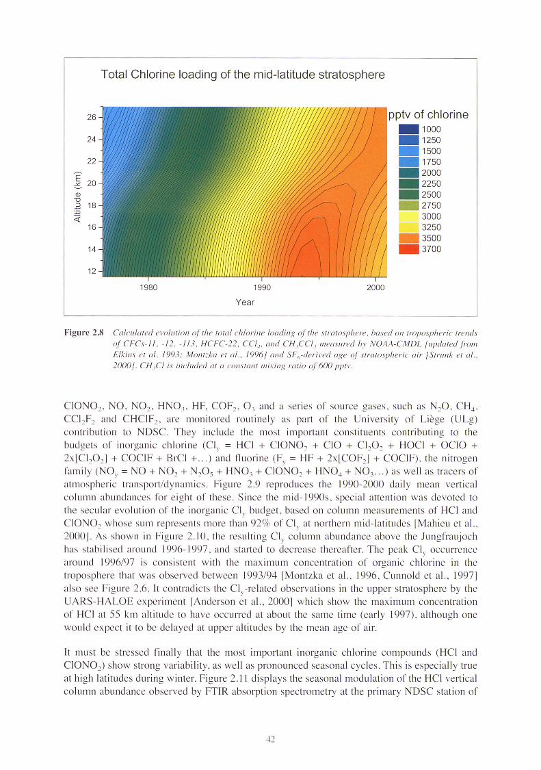
3.6 ppbv of chl orine, while at 27 km altitude thi s is ex pected to happen about fi ve years later with the max imum being at about 3 .5 ppbv, as shown in Figure 2 .8. As the mean time needed to transport air fro m the troposphere to a g iven location in the stratosphere increases w ith altitude (as can be seen fro m observation of the age of air), a time delay of about 3-4 years between the co lumn max imum of CIY and the tropospheric max imum of CCIY is ex pected . However, thi s contrad icts the CIY-re lated observations in the upper stratosphere (where the time de lay should be larger) by the UARS-HALOE ex periment [Anderson et a l. , 2000] which show the max imum concentrat ion of HCI at 55 km altitude to have occurred at about the same time (earl y 1997) as the max imum of the C IY column . The reason fo r the observation of a very earl y and very sharp max imum in HALOE HCI at 55 km is currentl y not understood [see also Waugh et a l. , 200 1 ].

Both sho1t -term , seasonal and secul ar characteri stics observed by FTIR spectrometry in the vert ica l co lumn abundances of HC I and HF above the northern mid-l atitude NDSC station of the Jungfraujoch (46.S°N, 8.0°E, 3580 m as l) have been reported fo r the peri od 1977-1995 in the previous EC Report [ 1997 , Figure 4. l , pp. 109] and in Zander et a l. [ l 996] . In addi tion ,

4 1

26

24

22

E 20 ~

(!) ""O

.2 18 ::E <(

16

14

12

Total Chlorine loading of the mid-latitude stratosphere

1980 1990 2000

Year

pptv of chlorine - 1000 - 1250 - 1500 - 1750 - 2000 - 2250 - 2500 - 2750

3000 3250

- 3500 - 3700

Figure 2.8 Ca/rnlcued e1 ,o/111io11 o/ 1he towl chlorine loacling of the stratosphere , based 011 tropospheric trends ofCFCs- 11 , -12. -11 3. HCFC-22 , CC!.; , and CH3CC/3 111eas11red br NOAA-CMDL fupda1ed.fi'0111 Elkins et al . 1993 : Mont -:.ka et al .. 1996/ and SF6 -derived age of stra tospheric air /Strunk et al. , 2000/. CH ;CI is i11c/11ded at a cons/Cl nt 111 i.ring rat io of 600 pp1 1·.

C IONO2 , NO , NO2 , HNO3 , HF, COF2 , 0 3 and a seri es of source gases, such as N2O , C H4 ,

CCl2 F2 and C HCIF, , are monitored routine ly as part of the Uni versity of Liège (ULg) contribution to NDSC. They include the most important constituents contributing to the budgets of ino rganic chlorine (C ly = HC I + CIONO2 + C IO + Cl 2O 2 + HOCI + OCIO + 2x [C l2OJ + COC IF + BrCI + ... ) and fluo rine (Fy = HF + 2x [COF2] + COCIF), the nitrogen fa mil y (NOY =NO+ NO2 + N2O5 + HNO3 + C IONO2 + HNO4 + NO3 ... ) as wel l as tracers of atmospheri c transport/dynamics. F igure 2 .9 reproduces the 1990-2000 daily mean verti ca l co lumn abundances for e ight of these . Since the mid- l 990s , spec ia l attention was devoted to the secul ar evo lution of the inorgani c C IY budget , based o n co lumn measurements of HCI and C IONO2 whose sum represents more than 92 % of C IY at no rthern mid-l at itudes lMahieu et al. , 2000] . As shown in Figure 2 .1 0, the res ulting C IY column abundance above the Jungfrauj och has stabili sed around 1996-1 997 , and started to decrease thereafter. The peak C IY occurrence around 1996/97 is consistent with the max imum concentration of organi c chl orine in the troposphere that was observed between 1993/94 [Montzka et al. , 1996 , Cunno ld et a l. , 1997] also see Figure 2.6 . Jt contradi cts the C IY-related observati ons in the upper stratosphere by the UARS-HALOE ex periment [Anderson et a l. , 2000] which show the max imum concentrati on of HCI at 55 km altitude to have occuJTed at about the same time (earl y 1997), a lthough o ne would ex pect it to be del ayed at upper altitudes by the mean age of a ir.

It must be stressed finall y that the most important inorganic chlorine compounds (HCI and C IONO2) show strong vari ability, as wel l as pronounced seasonal cycles . This is especia ll y true at hi gh latitudes during winter. Figure 2. 11 di sp lays the seasonal modulati on of the HC I verti cal co lumn abundance observed by FflR absorpti on spectrometry at the primary NDSC stat io n of

42

-"'E ~ (.) ~ 0

É. w u z < C z :, cc < z :!E :, .J 0 u

NDSC-RELATED MEASUREMENTS AT THE JUNGFRAUJOCH

1.4

~ 1.2 IO

~ 1.0

"' 0 0.8

6.0 •

- ' ~ 5.0 ,s • w • ' -;:; 4.0

~ 3.0 • 2.0

•

1.0 f-----+--------J'"-----+-----+---+-----+---+-----+---+----+---1

~ 5.0 w 5 4.0

J: 3.0

2.0

• 1 1 ' ••

:! i .fi:t..stit f-:;:i..~..i~~f ti~{Af,;ï • • 2.5 f-----+-------+-----+---+-----+---+-----+---+-. ---+---1

C • in 2.0 t • w • 1 • ' • 1 [

1.5

(' iL • • .: :,._ ... ~.JA.._ J,~ ..... __ tÂ.,. _.!~ 1.0 ... ._t111111-.r-:,.•.-.....,.. .. ,. ...... ~~· ... , . ... . . . 0.5 ~-~--"~--'---~---'------'---~----'----L---------L----'

1990 1991 1992 1993 1994 1995 1996 1997 1998 1999 2000

CALENDAR YEAR

Figure 2.9 Sample data of vertical column abundances of eight species recorded at the Jungfraujoch as part of the ULg contribution to NDSC-related activities on stratospheric changes. [Updated from Mahieu et al., 2000}.

43

7

lnorganic Cl above Jungraujoch 6 June to November monthly means

N

E Cly ~ u Q)

0 5 E

"' 0 .,-

~ ~

, • • w 4

0 • z / î <( ,, 0 / z / HCI ::::i 3 / (D / <(

z • 2 ::::i _/ 2 0 0 CION 2

•

----- CIO

0 1984 1986 1988 1990 1992 1994 1996 1998 2000

CALENDAR YEAR

Figure 2.10 The evolution of the burclens of HCI and CION02 above the Jungfi·aujoch, basecl on June to November monthly mean vertical column abundances (to avoid large winter-spring variability). The reportecl Cl,, inclue/es a CIO background load derived from mode[ calculations. [ Updated from Mahieu et al., 2000].

Ny-Âlesund/Spitsbergen (79°N, l 2°E, 10 m as!) since March I 992 [Notholt et al., 1997a, 1997b]. These data further show significant variability due to the influence of heterogeneous chemistry inside the polar vortex. This variability leads to great difficulties in assessing long­term trends during winter from such data sets. Nevertheless and despite the difficulties generally associated to monitoring activities in polar regions, good long-term measurements are starting to build up at the high-latitudes stations of the NDSC (see Box). This concerns in particular the active chlorine species CIO, measured by the microwave technique [Klein et al., 2000a], and OCIO now measured on a quasi-routine basis by UV-visible spectrometers [FrieB et al., 1998; Otten et al., I 998).

44

8•1015 ,-----,--.---,-----.--.------r--.---r--r--.----r-----.--.-----r---.----,------,---.--r-----.--.-----r--.---,,--,--.------r--.--.----.---r-ir-r--.----.----.--,

;;;- 6•1015 E ü

ü a> 0 E ~ 4•1015 E :::i 0 ü

ro ....... 0 z; 2-1015

I

0 '---'----'----'----..1........J-----'----'---'--.L.....J.-'--'---'--L.......L---'--'--..1........J-----'----'---'---'----'--'--'---'--L.......L---'--'---'-----'--'--'-~

0 100 200 Day of year

300

Figure 2.11 Seasonal variation observed in HCl total columns above Ny-Alesund, Spitsbergen (79°N, ]2°E, JO 111 asl) since March 1992 by FTJR spectrometry. [Updatedfrom Notholt et al., 1997a].

EUROPEAN CONTRIBUTION TO THE NDSC

After a decade of forma} activities, the NDSC has reached routine and reliable operation of a series of specific instrument types (e.g., Dobson and Brewer, UV-Visible, FfIR, Lidar, Microwave, Ozone- and Aerosol sondes, spectral UV). Its dual goal of observing and understanding changes in the stratosphere from as many as five primary stations and over forty complementary sites has required rigorous quality control procedures based on regular instrument inter-comparisons and calibrations, as well as on validation activities of retrieval algorithms and multi-dimensional chemistry-transport models.

In terms of field observations, the European contribution to the NDSC has continued to increase, with active operations currently performed at three primary stations and at over 20 complementary sites (see Figure box 2.1). Related assimilation/modeling activities have also become more attractive and substantial, as data sets for an increasing number of atmospheric constituents extend over longer time periods and become available as validated products at the dedicated NDSC- Data Host Facility of NOAA (USA) and at NILU (Norway) (see NADIR web page for further information: <http://www.nilu.no/projects/nadir/>). A complete description of NDSC objectives, structure, operation, data archiving and related protocols and publications can be found at the home web page <http://ndsc.ncep.noaa.gov/>.

45

1 NDSC Pnmary Sites

" NDSC Complementary Sites

,JO'

-6()'

NDSC Sites 900_·- -------------------~ ,90·

' ~ -1 i"

" I', ,\· i_

¼>, ,

.& Sa..,ra

- Kerguelenls:and  Cam:ibe lsand ,lnactr.e, .&

Macquanels:ana Â

- -6()'

•► ::i ,, '1' -90' ~--------- ------ ----~ -90'

Figure box 2 .1 Map shmving 1he global dis1ribu1io11 of prinrary and co111ple111e111ary SIC/l ions of 1he Nenvork for 1he De1ec1io11 of S1ra1ospheric Change . Europe has a s1rong involve111e111 in 1he NDSC. 1vi1h opera1io11 s being rnrre111/y pe1fonned al 3 primary si1es and over 11ven1y co111p/e111 enwry .1·i1es .

A ltho ugh it remains committed to monitoring changes in the stratosphere , with an emphas is o n the long-te rm evo lutio n of the ozone layer (decay, stabili sati on , recovery, .. . ), the NDSC has worked on ways to adapt progress ively to new cha ll enges ari s ing from advances in sc ientifi c understanding of environmenta l problems and to sc ientifi call y justified implementati ons resulting from po liti ca l developments . Amo ng the latter are the amendments and adjustments to the Montrea l Protocol and the more recent Kyoto Protoco l ( 1997) seeking stabili sati on of substances with large Greenhouse Warming Potenti a ls that a lter the radi ati ve fo rc ing of the climate system.

As pait of its in vo lve ment in the NDSC , Europe has played an acti ve rote in developing or improving several important aspects of the techniques operated within the network. M ost notably these have inc luded the optimisation of new profiling techniques applied to FrIR observatio ns and the ir sc ientific ex plo itation [Me llq vist et a l. , 2000], the development within the EMCOR project of new hi ghl y sensiti ve microwave techniques to measure stratospheri c minor constituents [Gerber et a l. , 2000; Maier et al. , 200 1], and the improvement of the sensiti vity and prec ision of the UV-visible DOAS technique fo r the measurement of key minor spec ies, in particul ar BrO [A li we ll et al. , 2001 a].

46

2.3.2 Bromine species

In recent years considerable progress has been achieved in our understanding of the chemistry and budget of stratospheric bromine, in particular within two projects supported by the EU during the THESEO campaign: HALOMAX (Mid and high latitude stratospheric distribution of long and short lived HALOgen species during the MAXimum chlorine loading) and Stratospheric BrO.

The budget of inorganic bromine in the stratosphere (Bry= Brü + BrONO2 + HOBr + BrCl + HBr + ... ) has been investigated by employing two methods: (a) the budget of organic source gas (Bry°rg) and (b) total bromine inferred from stratospheric BrO measurements using a modelled BrO/Bry partitioning (Br/n) [Harder et al., 2000; Pfeilsticker et al., 2000a]. For early 1999 these studies revealed that (Br/n) has a mixing ratio of 1.5 pptv in air just above the local Arctic tropopause (approx. 9.5 km), whilst at 25 km in air of 5.6 year mean age it was estimated to be 18 .4 ( + 1.8/-1.5) pptv from organic precursor measurements, and 21.5 (±3 .0) pptv from BrO measurements and photochemical modelling, respectively [Pfeilsticker et al., 2000a].

Spectrometric BrO observations from balloons, together with measurements of the age of the probed air masses obtained through simultaneous measurements of long-lived source gases of known atmospheric trend, such as CO2 or SF6 , provide new information on the trend in stratospheric bromine [Pfeilsticker, 2000]. Figure 2.12 displays the situation. As expected, the total stratospheric bromine inferred with the organic bromine method closely follows the measured trend of the tropospheric bromine-bearing sources gases, except for the Schauffler et al. [ 1998] data that is only a proxy for stratospheric bromine content. Total bromine inferred with the inorganic method also follows this trend, but it is 1-2 pptv larger, possibly because the organic bromine method does not account for a suspected influx of inorganic bromine into the stratosphere [Fitzenberger et al., 2000; Harder et al., 1998, 2000; Ko et al., 1997; Pfeilsticker et al., 2000a; Sturges et al., 2000]. The compilation thus provides evidence that the stratospheric bromine has increased from about 16-20 pptv (i.e. by about 25 % ) during the decade (1987-1996). Primarily this increase in stratospheric bromine is due to the increase in the atmospheric content of the halons H-1211 (by about 250%), H-1301 (by about 250%), H-2402 (by about 190%), and H-1202 (by about 200%) [Fraser et al., 1999].

Measurements of the surface concentrations of CBrClF2 , CBrF3 , CBrF2CBrF2 and CBr2F2

(respectively halons -1211, -1301, -2402, and -1202) have been made at the University of East Anglia (Norwich, UK) based on air from the CSIRO Cape Grim air archive [Fraser et al., 1999]. These analyses show that total bromine in halons has increased by a factor of 10 since the late 1970s and continues rise, largely because of the ongoing growth of halon-1211. Despite ceasing production of H-1211 and H-1301 in the developed world at the end of 1993 under provision of the Montreal Protocol, possible causes for the continued increase of halons are releases during the 1990s from the large halon "bank" that accumulated in developed countries during the 1980s and increased production of H-1211 in developing countries [WMO, 1999]. Hal on increases over the next few years could del a y the time of the currently expected total organic bromine maximum in the troposphere, and could cause the abundance of equivalent chlorine (see Section 2.3.3) to decline more slowly than predicted. It is therefore of great importance to pursue the monitoring of tropospheric and stratospheric bromine loadings during the upcoming decades in order to assess its impact on stratospheric ozone under conditions of reduced chlorine loading.

47

26

24

---> ...... 22 o..

o.. .._... Q) C 20 E 0 ,._

18 CO (.)

ï::::: <l) 16 ..c o.. +CH Br Cl J; (/) n m y X a, 0 ...... 14 CU ,._ ......

(.f) + Halons -CU 12 ...... 0

1---10 CH

38r - - . - -

8

1986 1988

6 0

00 ~ ~~-~~~

- -- -/

- - .

1990 1992 1994 1996

Year of Stratospheric Entry

tropical troposphere

average

tropical upper troposphere

1998 2000

Figure 2.12 A recent history of the total organic and inorganic stratospheric bromine inventory [updated ji"Oln Pfeilsticker, 2000]. The dotted magenta fine corresponds ta a global averaged CH3Br swface concentration of JO pptv. The dashed blue fine clenotes the aclded trend of surjètce ha/on concentrations (H-1211, H-1301, H-2402, and H-1202). The so/id blue fine denotes the added tropospheric inventory of short-lived bromocarbons (C,,H,,,Br __ Ct,) [Fraser et al., 1999]. The blue fïlled squares are nzeasurements of total organic bromine in the upper troposphere and lm1'er strato~phere by Wamsley et al. [ 1998 J and Schauff7er et al. [ 1998, 1999 ]. The open circ/es de note the total inorganic bromine inferred from stratospheric BrO measurements and photochemical cafculations, accounting jàr the BrO!Br, ratio [Harder et al., 1998, 2000; Pfeilsticker et al., 2000a]. The years when these measurements were made are given next to reported data.

The capabilities of remote sensing instruments to monitor BrO from the ground [Richter et al., 1999], balloon, aircraft and space using UV-visible spectroscopy have been successfully assessed within the Stratospheric Brü project [Van Roozendael et al., 2000]. This will form the basis of the future observing system for long-term global monitoring of BrO (i.e. 60% of the available inorganic bromine during daytime). As an example, Figure 2.13 shows time series of BrO differential slant columns measured at six European stations of the Stratospheric BrO ground-based network from 1998 until mid-2000. These observations have been used to characterise and test against 3-0 chemical transport simulations the shmt-term, seasonal and secular variations of BrO at various latitudes [Sinnhuber et al., 2000a, 2001].

48

.p.. \0

_ 3.5 NE

~ 3

" 0 E 2.5 ..,

-0

• ~1.5 ~-~ ~ 0 1 U 1 ' ~ •

Cl) ' ' Q 057 ...... Ill O I J~ M A

N- 3.5 E ~ 3

" 0

.., E 2.5 -0

0

·h

M J J

1998

~15 1 ~· •'· 0 1 ~ · • u r,.,, •• ,9. Cl) .. , •

o 0.5 •

~ 0

JFMAM

N-3.5 ~--­E

~ 3 0

}2.5

Ny-Alesund , 79°N

Meas. AM Meas. PM Model AM

- Model PM

~ ~ ~

:·"'·

~ ,,· ... ' , ._ 1

f.-u • •• ' t"~ . ~ ~ \

A , N, DJ J~' MA M J J A S~D[ J , F\ M

!

Date 1999

Kiruna , 68°N

Meas. AM • Meas. PM

- ModelAM - Model PM

Date

Andoya , 69°N

-~ Meas. AM • Meas. PM

- ModelAM - Model PM

,1~ : 0

~ 1 ! ,,""

~ ~ -~ 0 0.5 t -

A M 2000

2000 A M

} 2 ?J~' ~O JJASO

1998

MA M J J A S Q 1999 D i J F M A M

2000

Date

3.5

"Ë ~ 3 0 E 2.5

~

-~ 2

3.5 NE

~ 3 0 E 2.5

~

-~ 2

0 "j' 1.5 0 "' 0 1 (J

~ 0.5

Q Ill 0

3.5 NE ~ 3

" 0 E 2.5

~

~ 2

0 <X>

·' "' e 0 (J

~ 0.5

Q Ill 0

Harestua , 60°N

Meas. AM Meas. PM Model AM

- Modal PM

1998 1999 2000 J FM AM J~ J AS ON Di J FM AM J J AS ON Di J FM AM

Date

OHP, 44°N

Meas. AM • Meas. PM

- ModelAM - Model PM

1998 1999 2000 FM AM J J AS ON D J FM AM J J A_ S~ J FM AM

1998

Date

Bremen, 53°N

~ ~

A S O N D J F M A

Date

· Meas. AM • Meas. PM

- ModelAM - Model PM

S O N D J F M

2000

Figure 2.13 BrO di.fferentia l slant colunlll benveen 90° and 80° SZA 111easured at six stations of the Stratospheric BrO network .fro111 1998 until May 2000. AM and PM 111eas11re111ents (b lue sy111bols) are co111pared to si11ntlations.fro111 the SLJMCAT 3-D 111odel (red lines) . The grey shaded areas indicate periods when the sun did not reach solar ::.enith angles of 80°. Twilight BrO 111eas11re111ents exhibit a latitude-depende111 seasonaliry 111ainly controlled by Fariations in stratospheric N02 .

[Sinnhuber et al., 2000a, 2001 ].

23.3 Total Equivalent Chlorine

In order to estimate how the future abundance of stratospheric ozone will respond to simultaneous decreasing chlorine amounts and increasing bromine from halons, the trends for both Cl- and Br-containing species must be considered. This is true despite the comparatively low atmospheric concentrations of bromine, because on a per-atom basis, Br has a much larger catalytic efficiency at destroying ozone than chlorine. The relative impact of bromine compared to chlorine upon stratospheric ozone is characterized by the so-called a parameter [e.g. Salomon et al., 1992). The values of a remain highly uncertain depending on a number of factors [Daniel et al., 1995), currently a mean value of 60 is being recommended by WMO [ 1999) when dealing with globally averaged ozone lasses. The total equivalent chlorine is defined at a given time as the amount of tropospheric organic halogen that will become (at some future time) reactive inorganic halogen available to participate in the ozone depleting reactions. It can be estimated by weighting tropospheric mixing ratios of individual compounds according to their relative decomposition rates within different regions, and by accounting for the different catalytic efficiencies of chlorine and bromine using the a parameter. Calculations by Montzka et al. [ 1996) indicate that total equivalent chlorine peaked for polar regions in late 1993 and early 1994, and decreased afterwards at a rate of -18±3 pptv per year. It should be noted that these numbers do not include the time lag between the troposphere and the stratosphere, which is a fonction of altitude, latitude and season. Continued increase of bromine loading due to emissions of anthropogenic halons could slow down this rate in the future.

2.4 TRENDS IN OTHER MINOR CONSTITUENTS

2.4.1 Water vapour and methane

Long-term changes of stratospheric water vapour are an important but still unknown parameter for the prediction of future changes of the ozone layer. Indeed, increasing water vapour concentrations could result in higher frequencies of polar stratospheric clouds and therefore delay the expected recovery of the ozone layer [WMO, 1999), especially if the build-up of greenhouse gases in the atmosphere results in a cooling of the stratosphere. Such a cooling could additionally be reinforced by the presence of increased water vapour amounts. These issues are further investigated in Chapter 5 of this report.

In the SPARC water vapour assessment [Kley et al., 2000), water vapour trends have been assessed. From a multi-decadal record of balloon launches over Boulder, Colorado, Oltmans and Hofmann [ 1995] and Oltmans et al. [2000] derived an increase of water vapour in the lower stratosphere exceeding 1 % per year over the period 1980-2000. The observed increase is similar at ail altitudes between 16 and 26 km and highly significant at ail levels above 16 km. Using ail published data sets, Rosenlof et al. [2000) assess a likely 1 % per year increase of water vapour in the stratosphere since the middle 1950s (2 ppmv in all). Up to a half of this increase can be understood as arising from the increase in tropospheric methane since 1950 (0.55 ppmv), since photochemical oxidation of methane in the stratosphere produces approximately two molecules of water vapour per molecule of methane. The reason for the remainder of the reported increase in stratospheric water vapour remains unclear.

Up to now, the European in situ measurement record of H20, only available since the 1990s, cannot be used for a similar analysis. lt is expected however that relevant data sets will become

50

sufficiently large within the coming years to follow the current changes. Unsuccessful attempts to identify a water vapour trend in the period 1992-2000 were recently reported by Schiller [1999] based on an analysis of available data sets of 2xCH4+H20 [Engel et al., 1996; Stowasser et al., 1999; Zoger et al., 1999a]. This quantity is expected to be less sensitive to regional dynamical changes than a single H20 measurement. This approach will be pursued in the near future as new observations become available.

The temporal increase of methane has also been investigated by FTIR spectrometry at several ground-based locations, i.e. in Europe at the NDSC stations of Ny-Âlesund and Jungfraujoch. The observations at Ny-Âlesund are performed with the sun as a light source, except during the polar night (October-February) when the moon serves as a source. Data on total vertical column abundance of CH4 above the Jungfraujoch have been gathered routinely since the mid-1980s, but similar "historie" measurements were also made in 1950/51; a consistent analysis of this ensemble indicates that the vertical column abundance of CH4 increased from 1.68 to 2.28xl0 19 molec cm-2 , or 35%, over the last fifty years. However, since the mid-1980s the rate of CH4 growth has slowed significantly, by over a factor of three (Figure 2.14), in line with findings from ground-level in situ investigations reported in Chapter 2 of WMO [1999].

2 .40 ,-----,,-------r------r-----r----r----.----.------.,..----,-----r-----r-----r----r----.----.------.,..----,~

-N

2.35

E 2.30 ü -cS Q)

o 225 E

CJl

~o :S. 220 C

E ::::l 0 2.15 u

CO +-'

~ 2.10

2.05

0

0

Jungfraujoch - CH 4 P-Normalised Daily Mean Columns

0

0

0

0

Q

0

-0.75% per yr

î î

-0.45% per yr

î -0.25% per yr

2.00 ~~~-~-~-~-~-~-~~-~-~-~-~-~-~-~----'-' 1985 1987 1989 1991 1993 1995 1997 1999 2001

Year

Figure 2.14 Time series of daily mean vertical column abundances of CH-1 monitored above the Jungfraiijoch from 1985 to 2000. Mean rates of increase during 1985-1990, in 1993 and in 1998 have been around 0.75, 0.45 and 0.25% per year. [Updated from Zander et al., 2000a].

51

2.4.2 Nitrogen species

The importance of nitrogen oxides for stratospheric ozone concentrations has long been recognised. NO and NO2 (NOJ can destroy ozone catalytically, but they can also reduce ozone depletion caused by reactive chlorine and hydrogen compounds by converting these gases into unreactive reservoirs such as ClONO2 and HNO3 . The source of stratospheric NO2 and other nitrogen compounds (collectively known as NOY) is N2O released at the ground, then destroyed in the upper stratosphere by reaction with O(1D).

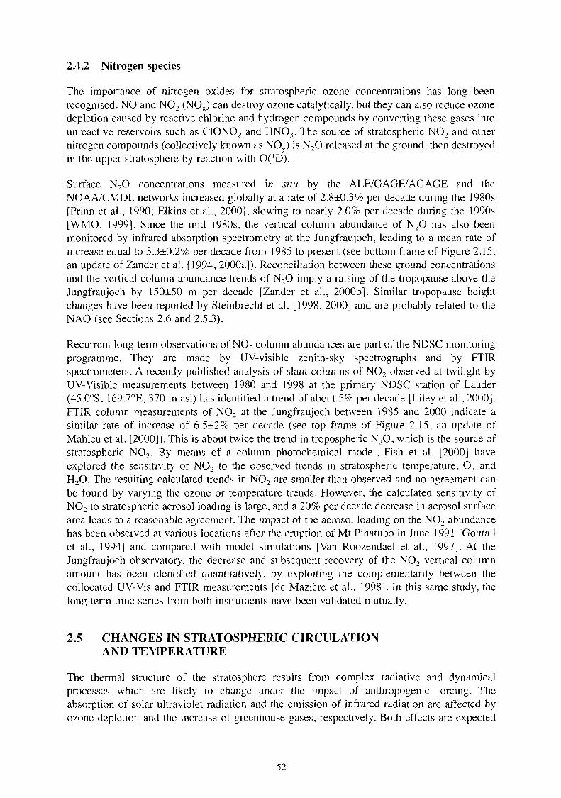
Surface N2O concentrations measured in situ by the ALE/GAGE/AGAGE and the NOAA/CMDL networks increased globally at a rate of 2.8±0.3% per decade during the 1980s [Prinn et al., 1990; Elkins et al., 2000], slowing to nearly 2.0% per decade during the 1990s [WMO, 1999]. Since the mid 1980s, the vertical column abundance of N2O has also been monitored by infrared absorption spectrometry at the Jungfraujoch, leading to a mean rate of increase equal to 3.3±0.2% per decade from 1985 to present (see bottom frame of Figure 2.15, an update of Zander et al. [ 1994, 2000a]). Reconciliation between these ground concentrations and the vertical column abundance trends of N2O imply a raising of the tropopause above the Jungfraujoch by 150±50 m per decade [Zander et al., 2000b]. Similar tropopause height changes have been reported by Steinbrecht et al. [1998, 2000] and are probably related to the NAO (see Sections 2.6 and 2.5.3).

RecmTent long-term observations of NO2 column abundances are part of the NDSC monitoring programme. They are made by UV-visible zenith-sky spectrographs and by FTIR spectrometers. A recently published analysis of slant columns of N02 observed at twilight by UV-Visible measurements between 1980 and 1998 at the primary NDSC station of Lauder (45.0°S, 169.7°E, 370 mas!) has identified a trend of about 5% per decade [Liley et al., 2000]. FTIR column measurements of NO2 at the Jungfraujoch between 1985 and 2000 indicate a similar rate of increase of 6.5±2% per decade (see top frame of Figure 2.15, an update of Mahieu et al. [2000]). This is about twice the trend in tropospheric N2O, which is the source of stratospheric NO2 • By means of a column photochemical mode!, Fish et al. [2000] have explored the sensitivity of NO2 to the observed trends in stratospheric temperature, 0 3 and H2O. The resulting calculated trends in NO2 are smaller than observed and no agreement can be found by varying the ozone or temperature trends. However, the calculated sensitivity of NO2 to stratospheric aerosol Ioading is large, and a 20% per decade decrease in aerosol surface area Ieads to a reasonable agreement. The impact of the aerosol loading on the NO2 abundance has been observed at various locations after the eruption of Mt Pinatubo in June 1991 [Goutai! et al., 1994] and compared with model simulations [Van Roozendael et al., 1997]. At the Jungfraujoch observatory, the decrease and subsequent recovery of the NO2 vertical column amount has been identified quantitatively, by exploiting the complementarity between the collocated UV-Vis and FTIR measurements [de Mazière et al., 1998]. In this same study, the long-term time series from both instruments have been validated mutually.

2.5 CHANGES IN STRATOSPHERIC CIRCULATION AND TEMPERATURE

The thermal structure of the stratosphere results from complex radiative and dynamical processes which are likely to change under the impact of anthropogenic forcing. The absorption of solar ultraviolet radiation and the emission of infrared radiation are affected by ozone depletion and the increase of greenhouse gases, respectively. Both effects are expected

52

-N

E (.)

- 6.0 (.) Q)

0 E 5.o L!)

0 ~ 4.0

C E ::J 3.0 0 ü

2.0 CO .......

Jungfraujoch - NO2 P-Normalised Monthly Mean Column

o e

0 0 Mean: +(0.62±0.19)% per yr

0 0

c9

0

0 0

0 1- 1 .0 l...-__JL.....---1----1.----'-----1....---'--...J..._-...J.... _ _L_ _ __.___..L-_..___,..___._____, _ __,

1985 1987 1989 1991 1993 1995 1997 1999 2001

-N 5.0 ,----,,----,----.---,--~---,--~--,----r--.----,---.,--..----.---,,----,

E (.) -(.) Q)

0 E

CX)

0

4.5

::S 4.0 C E ::J

8 3.5

CO ....... 0

Jungfraujoch - N2O P-Normalised Monthly Mean Column

Mean: +(0.33±0.02)% per yr 1- 3 .0 .___.____,'----'----'-----L---'----'------'---'--......_ _ _,___....___.,___..___.____,

1985 1987 1989 1991 1993 1995 1997 1999 2001

Year

Figure 2.15 Time series of monthly mean total vertical column abundances of NO2 (top frame) [update from Mahieu et al., 2000] and N2O (bottom frame) [update from Zander et al., 2000b] observed by FTIR spectrometry above the Jungfraujoch since 1985. Note the large reduction of the NO2

column after the 1991 volcanic eruption of Mt Pinatubo [de Mazière et al., 1998] and the seasonal modulations affecting bath compounds; also the different vertical scale units of both frames.

to lead to a cooling of the stratosphere. Changes in the aerosol loading and in water vapour also affect the radiation budget. The transport of heat and mass by the general circulation can be affected by changes in radiatively-induced thermal gradients as well as by changes in the absorption of waves propagating up from the troposphere.

An extensive review of stratospheric temperature trends by Ramaswamy et al. [2001] came to the overall conclusion that the stratosphere has cooled considerably from the mid-1960s to the mid-1990s, most strikingly since 1979. It is generally agreed that a cooling trend is observed,

53

but it is still unclear how much can be attribu ted to anth ropogenic fo rc ing. The large dy namica l vari ability in the no rthern po lar reg ion during late winte r and spring makes re li ab le de tecti on of trends in the Arcti c winter difficult - e ithe r in the observati ons or in model s imulati ons (see C hapte r 5) .

2.5.1 Natural Variability

The large inter-annual vari ability of the northern hemisphere in late winte r and spring over polar latitudes is due to the occurrence of stratospheric warmings . T he 30 hPa temperature dev iations from the long-term monthl y mean in January 1999 and January 2000 (Figure 2 .1 6) impress ively show the contrast between a warm and a co ld winter. Since the essenti al mechani sm fo r these warmings is the upward propagati on of planetary waves from the troposphere and the ir interaction w ith the ex isting stratospheri c fl ow, the occurrence and magnitude of thi s natu ra l variability is influenced by vari ati ons in both the troposphere and the stratosphere . Factors influencing the state of the winter-time stratospheri c circul ati on will now be described .

• During its easterl y phase the Quasi-Biennial Oscillation (QBO) offers ideal conditi ons fo r the propagatio n of planetary wavenumber 1, leading to a strengthening of the A leuti an anti cyclo ne and an amplificati on of po leward transport , thus to a more di sturbed and warmer Arcti c. During the westerl y phase of the QBO the po lar vortex tends to be co lder and more stable . G ray et a l. [2001] have shown that thi s sensiti vity of the polar vortex to the equ atori a l wind direction is influenced by the phase of the QBO in the upper stratosphere and not just in the lower stratosphere, as prev iously assumed . Further deta il s abo ut the QBO may be fo und in the rev iew by Baldwin et al. [200 l ] .

JAN 99

-10 -7 .5 -5 -2.5 0 2.5 5

30 hPa t.T

30 hPa t.T in K

FU Berli n Ana lysis

-15 -12.5 -10 -7 .5 -5 -2.5 0 2.5

Figure 2.16 JO hPa te111perature devia1ionsjim11 !he /011g- tem1111eans in Ja1111ary 1999 and 2000; dots indicate

!he No r1h Pole and the nearest g rid points 10 the observing stations Nv Alesund. Kiruna. Oslo ,

Berlin , and Bordeaux (FU Berlin analvses) .

54

• The solar cycle modulates this expected connection between the QBO and the winter-time stratospheric circulation, weakening it during sunspot maximum. Labitzke and van Loon found stati stically significant differences between the east and the west years of the QBO when they considered periods of sunspot minima , whereas during high so lar activity the w inters in the west phase of the QBO tend to be disturbed and are often connected with major mid-winter wa1mings [Labitzke and van Loon , 2000; van Loon and Labitzke, 2000]. This results in positive coITelations between the 30 hPa geopotential heights and the 10.7 cm solar flux and in positive height differences between maxima and minima of the solar activity over the Arctic during the west phases of the QBO (Figure 2.17, lower panels) . During the east phases (Figure 2.17 , upper panels), negative correlations and negative height differences illustrate a more disturbed polar vortex in qui et sun periods, as expected from the QBO connection above.

Solar Cycle; 30 hPa Height (Jan+Feb)/2 1958-2000 FUB

corr Height Diff. (gpm)

East (n =1 8)

corr Height Diff. (gpm)

West (n=25)

Figure 2.17 Correla1io11 s be/1\'een the 10.7 C/11 solar.flu.r and mean 30 hPa heights in January!February fo r 1he period 1958-2000 (le.fi, shaded are correlations above 0.5) and heigh1 differences between so/ar 11wxil11a and 111i11i111a (rig/11 ), grouped into the years in 1he east and ive.\"/ phase of the QBO. / Updated fro111 Labir:.ke, 2001 } .

SS

• During a warm event of the El Nino/Southern Oscillation (ENSO), increased convection in the equatorial belt leads to a stronger upward motion of air and to a cooling of the tropopause and lower stratosphere in the tropics. Although this mainly results in dipole patterns over Indonesia and the central Pacifie Ocean [Randel et al., 2000], there are also signais in the zonal averages of lower stratospheric temperatures over the tropics. The weaker temperature gradient to high latitudes causes weaker westerly winds, a stronger Aleutian anticyclone, and a weaker vortex. Warm ENSO events often result in major midwinter warmings and the associated mixing of air in the polar region with air from mid­latitudes while cold ENSO events are mostly connected with a cold and intense polar vortex [Labitzke and van Loon, 1999).

• The North Atlantic Oscillation/Arctic Oscillation (NAO/AO) modulates the stratospheric wintertime circulation; this is described further in Section 2.6.

• Finally, volcanic eruptions, injecting gaseous material into the stratosphere which forms sulphate aerosols, additionally disturb the stratospheric temperature and circulation pattern for some time after the event. The aerosol loading after the three eruptions of Mt Agung (1963), El Chichon (1982), and Mt Pinatubo (1991) (see Section 2.8) caused a strong warming of the tropical stratosphere almost immediately (through direct absorption of Iong­wave radiation). Pawson et al. [1998] have shown that the observed negative trend in the 30 hPa annual mean temperatures over the northern hemisphere seems to have occurred in a stepwise manner following the volcanic eruptions of El Chichon and Mt Pinatubo.

2.5.2 Long-term changes

The trends in annual mean, zonally-averaged temperatures and geopotential heights in the northern hemisphere lower stratosphere for the period January 1965 to December 1999 are shown in Figure 2.18. The temperature trends are negative at ail latitudes with maxima in the subtropics and in the polar region slightly above 50 hPa. Changes in the geopotential heights are positive in the lowermost stratosphere sou th of about 60°N, reflecting the vertically diminishing positive temperature trend in the troposphere, and negative to the north, becoming more so with height. This meridional distribution of height trends indicates a strengthening of the westerly winds at mid-latitudes.

Trends in the annual means in Figure 2 .18 are the residual of different trend patterns in different months. In winter especially, the influence of natural variability leads to rather low statistical significance for stratospheric trends. Moreover, calculated trends strongly depend on the beginning and the end of the time series, e.g. the year 1979, when satellite data became available and when the ECMWF ERA-15 data begin, coïncides with a maximum in solar activity. Figure 2 .19 shows striking differences in the linear trends calculated for two different time periods of monthly mean 50 hPa temperatures - the level of the strongest cooling for the period 1965-1999 in Figure 2.18. The trends are negative for the longer period over the whole of the northern hemisphere, but weaker than for the shorter period, and strongest deviations are observed during the winter and spring months.

2.5.2.1 Winter and Spring

The longest data set available for stratospheric temperatures is that for the 30 hPa monthly mean temperatures over the North Pole from the FU Berlin analyses for the winters

56

ro o... ..c

50

100

30

ro 50 o... ..c

Trend Annual Mean (January 1965-December 1999) Temperature (°C per decade) Trend Annual Mean

(January 1965-December 1999)

10°N 20°N 30°N 40°N 50°N 60°N

I •

I ,I / / i i

.,.' i

\ \

70°N

Geopotential Height (gpdm per decade)

\

80°N

100 ______________ .......__ __ ___.__~

10°N 20°N 30°N 40°N 50°N 60°N 70°N 80°N

Latitude

90°N

90°N

Figure 2.18 Annual mean , w nally a veraged trends of tempera/ure (top) and of geopotential heighl in decametres (bol/0111 ) over the nor!hern hemisphere between 100 and 30 hPa jimn FUB da/a for the period 1965- / 999. / Updated jim11 Labitzke and van Loon , 1994/.

57

Q) '"O

:::J +-' +-' m

Q) '"O :::J +-' +-' m

90°N , ,

80°N

70°N

60°N

50°N

40°N

30°N

10°N JUL

90°N

80°N --·

70°N

60°N

50°N

,,

50 hPa Temperature Trend (°C per decade)

1965-2000 , 1 1 1 1 ' ' ' 1 1 1 1 ' '· , 1 1 1 1 '

-, _______ -0.5

, 1 1 1 1 1

' 1 1 1 1 1 , 1 1 1 1 1 i \ , 1 1 1 ' 1

', , 1 1

' ' ' 1, , 1 1 ' , 1

\,' , 1 1 ,

' ' ,.-0.5 , 1 1 , , ' ,

1 1 , , ' , 1 1 ,,,, , ' ,, ·, , 1 ' ,' \ ,, ' ,' 1 1 ,, ' ' ' ,/ ' .. ,........ ,/ ' / ' -, ' ' ' ' ...... _, ' '

,, \\ ' \ / ,,

1 ,,' 1 ' -1

\\ ,,,,,' -,

1 --1 --1 ', 1 \ ' ,,,, ' 1 ' ' 1 ' ' 1 \ 1

' , 1

' ' , 1

\ 1, 1 , ,

1 ,,_ , 1 , / ' ,,l -- ' -- ,, 1 --- ,, 1

-------- 0 5'' 1

···, -o.5----------· ' \ ,, ... _. ,, .................. __ ,, ,,

AUG SEP OCT NOV DEC JAN FEB MAR APR MAY JUN JUL

,,----------1 ,/ ,,

_,

1979-2000

2

' 1 1

' ' ' ' ' 1 • -, ______ _

-------·-1 .• ___

40°N ... ,,\

\ ' ' ' 1

30°N 1

' /

20°N ,,,,,,.,,,

,,,, ·'

AUG SEP OCT NOV DEC JAN FEB MAR APR MAY JUN JUL

Month

Figure 2.1 9 Mon!h ly 111ean , ::.unal/y m·eraged 1e111peralllre !rends ar 50 hPa uver 1he nor!hern he111isphere fo r Iwo diffe ren1 periods : / 965-2000 (!Op) and / 979-2000 (bo110111 ) jim11 FUB daw. [Upda1ed f imn Labi1::.ke and van Loon , / 994}.

58

1955/56-1 999/2000. These data exhibit a stati stically significant linear trend onl y in November: - 1 .2 K per decade [Labitzke and Naujokat, 2000]. The w inter months December, January, and February show sli ghtl y negati ve but not significant trends, and in March and April almost no trend at a il is di scernible.

A closer look at the monthly mean temperatures of forty-five w inters reveals that in earl y w inter a clear change in temperature and circulation took place . In November/December, Canad ian warrnings were frequentl y ob erved in the years until 1981/82, but have been almost absent fo r the las t e ighteen winters . This points to changes in tropospheric conditions, s ince the Canad ian warmings are connected with intensification of the Aleuti an stratospheri c high/tropospheric low. While almost a il Novembers have been cold in the past e ighteen years, December has been more variable : very cold conditions were observed in some years , but also two major warm ings took place ( 1987 and 1998), a feature not observed in the thirty-two years fro m 1952- 1985. T hi s is refl ected in the pos iti ve trends for December for the period 1979-2000 in F igure 2. 19. During the latter peri od six major warmings took place in January and eight in February, compared with one in January and three in February from 1986 onwards . Indeed , there was a period of seven winters from 1991/92- 1997/98 without major warmings. A possible ex planati on fo r thi s is that the QBO was in a westerl y phase during the fo ur w inters fro m 1993- 1996, a sequence not prev iously experienced . In addition, solar activity was low during these winters.

Late w inter/spring is an important time since a long-las ting cold vortex favo urs ozone destruction , while earlier break-ups of the vortex are connected w ith transport of ozone in to the polar reg ion . F igure 2.20 shows the 30 hPa monthly mean temperatures fo r March at the North Pole fro m 1956-2000 . Linear trends have been calcul ated fo r three di fferent periods: fo r the complete series the trend is zero, fro m 1956-1 979 it is pos iti ve (and s ignificant) , and it is strongly negati ve (again s ignificant) fro m 1979-2000 .

(OC) Temperature Trend March POLE 30 hPa

-40 @ 1979-2000

-45

CD Tm= -59 n = 24 - 50 sigma= 7.6 Trend = 2.06°C/dec. Prob = 63%

-55

@ Tm= -56 8 - 60 n = 22 sigma= 78 2 Trend = 5.95°C/dec. Prob = 97% -65

@ - 70

Tm=-5675 n = 45 sigma= 7.9 - 75

CD 1955-1978

Trend= 0.02°C/dec Prob = 2%

1955 1960 1965 1970 1975 1980 1985 1990 1995 2000

Figure 2.20 Time series of 30 hPa mon th/y mean tempera/ures at the North Pole in Ma rch, / 956-2000 Ji-o,n FU Berlin da ta; linear trends ha ve been computecl fo r three different periods . / Upda ted .fi-0, 11 Labit~ke and van Loon, 1999}.

59

Zonally and monthly averaged data possibly obscure the occurrence of extremely cold regions which are often associated with amplified planetary waves. The inspection of daily data revealed that the minimum temperatures reached on any day at any location of the northern hemisphere show a negative trend, at least until the winter 1996/97 [Pawson and Naujokat, 1997). During the three winters of the middle 1990s extremely cold periods of long duration occmTed and the coldness persisted into the late winter [Pawson and Naujokat, 1999). The indicated cool ing trend there was interrupted by the two warm winters 1997 /98 and 1998/99, but continued by the winter 1999/2000 which was one of the coldest on record since the Berlin northern hemispheric temperature analyses began in 1964/65. Figure 2.21 shows the number of days for each winter season on which the minimum temperature was below the thresholds for the formation of Type 1 Polar Stratospheric Clouds (NAT PSC). In the lower part of Figure 2 .21 , the area of possible PSC formation over the northern hemisphere is shown, integrated for each winter. The linear trends reported before [Pawson and Naujokat, 1997] are slightly reduced when adding the recent years to the record, but still persist.

2.5.2.2 Summer and Autumn

The relatively undisturbed stratosphere in summer and autumn, when the predominantly easterly winds prevent the upward propagation of planetary waves from the troposphere, is

100 (a)n,. 50hP~ Cl) 80 >, 0 -0 -0

0 z

Cl) >,

60

40

20

0 \4 .• ___ ..,,.__ ~ 1965 1970 1975 1980 1985 1990 1995 2000 /66 /71 /76 /81 /86 /91 /96 /01

50hP 0 1 5 -0 .

X I z

0.5

0 _.,__ ___ _,_...:-__ ._..a.:..,.._..,_ ______ -:.-.,,

1965 1970 1975 1980 1985 1990 1995 2000 /66 /71 /76 /81 /86 /91 /96 /01

season

100

80

60

40

20

0

(b)nT

"'

:c:

"-

~

30hPa '

"' ~

" ~ ..

F-•

1 • 1965 1970 1975 1980 1985 1990 1995 2000 /66 /71 /76 /81 /86 /91 /96 /01

30hPa 1.5

0.5

0 --""''-,,----'-,...;-----.-----.----------1965 1970 1975 1980 1985 1990 1995 2000 /66 /71 /76 /81 /86 /91 /96 /01

season

Figure 2.21 Number of days (a, b) with minimum temperatures below the PSC thresholds for NAT and ice at 50 and 30 hPa and the integral of the areas o_f'possible PSC formation (c, d) ovcr the winter at 50 and 30 hPa for the winters l 965!66-1999/2000 /rom FU Berlin analyses. [ Updated jimn Pawson and Naujokat, 1999].

60

Temperature Trend July POLE 30 hPa (OC) ~---------------------~

CD Tm = -38.4 _

36 n = 25 sigma= 0.7 Trend= 0.04°C/dec. Prob = 16% - 3 7

-38

Tm= -39.7

;;;;; = 1 1 - 39 Trend = 1.32°C/dec. Prob = 99%

-40

G) -41

Tm= -39.0 n = 46 sigma=1 .1 -42 Trend = 0.56°C/dec. Prob = 99%

(3) 1979-2000

G) 1955•2000

CD 1955-1 978

-43 -'-T---~-~--~-~--~ -~-~,----,--~~ 1955 1960 1965 1970 1975 1980 1985 1990 1995 2000

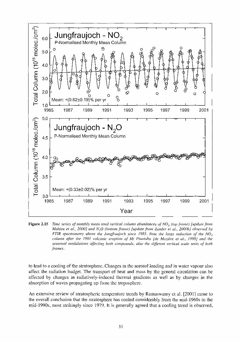
Figure 2.22 Same as Figure 2 .20, but f or July.

better suited to trend detecti on . Considering again the longest avail able peri od fro m 1955-2000 , the 30 hPa monthl y mean temperatures at the North Pole for Jul y (Figure 2.22) shows a stati sti call y significant negati ve trend of about 0.5 K per decade. The linear trend calcul ati ons fo r the two sub-peri ods 1955-1 979 and 1979-2000 show more cooling in the latter period , thus suggesting that at least part of the observed strong cooling in the Arcti c w inter since l 979 might be attributed to a reali stic trend in spite of the natural vari ability.

F igure 2.23 shows the northern hemispheri c di stribution of temperature trends per decade at 50 hPa in summer (average of June and Jul y) fo r the peri od 1964-2000. The negati ve trends in this map are signifi cant on the 99% level and are quite robust against diffe rent data peri ods.

2.5.3 Changes in the lowermost stratosphere

Changes to the c ircul ation of the main part of the stratosphere affect the Brewer-Dobson c ircul ati on and the re-di stribution of ozone around the pl anet, thus hav ing a first-order influence on ozone. However, the dynamics of the troposphere also has a direct influence on the lowermost part of the stratosphere since short-wavelength Rossby waves can propagate into thi s region. In recent years it has become clear that mi xing of subtropical, ozone-poor air into the mid- lat itude lower stratosphere acts to reduce the ozone concentrati on there [O 'Connor et a l. , 1999 ; Orso lin i et a l. , 1995a; Vaughan and Timmi s, 1998] and that thi s mi xing is contro ll ed by Rossby-wave break ing [Peters and Waugh, 1996] . There is some ev idence that the frequency of Rossby wave-break ing events is increasing [Hood et a l. , 1999] and that layers of ozone-poor air in the lower stratosphere have become more common [Re id et al. , 2000], although thi s may be another manifes tati on of the North Atlantic Osc ill ation (see Section 2.6). Indeed , Hudson and Fro lov [2000] analysed trends in TOMS total ozone according to the

61

Figure 2.23 Linear !rend of 50 hPa 11 10111h/v 111ean 1e111pera1ures in June/Julv (K per decade) over 1he non hem he111isphere for 1he period / 964-2000 .fi-0,11 FUB da/a.

meteoro logical reg ime of each measurement (tropi cal, mid-l atitude and po lar), and fo und no trend at a il in tota l ozone within each reg ime. The ir conclusion was that ozone changes in the northern mid-l atitudes are caused by the systematic northward movement of the po lar and sub­tropical jetstreams.

A 30-year data record ( 1967- 1997) of vertica l te mperature and ozone profi les measured at the Meteoro log ica l O bservatory Hohenpe issenberg (47 .8°N, l l .0°E) was analysed w ith respect to trends lSte inbrecht et a l. , 1998]. They fo und that the tropopause height rose 150± 70 m per decade over the peri od . This he ight shift is corre lated w ith an observed warming of the troposphere , fo r example , 0 .7±0 .3 K per decade at 5 km altitude. Basecl on the we ll known anticorre lati on between tropopause he ight and ozone column it was specul ated that the increase in tropopause he ight coulcl contribute approx imately one third of the mid-latitucle ozone reducti on. This result however could be re lated to the North Atl antic Osc ill ation (see below).

2.5.4 Changes to the Arctic polar vortex

The Arctic po lar vortex usua ll y form s in November-December and breaks up in March-April. There are, however, large differences between indi vidual winters in vortex du ra ti on, coldness and strength. Figure 2 .24 presents the break-up dates of Arctic polar vortices and average vo1tex

62

strengths in the 1980s and 1990s, derived from ECMWF analyses using the method of Nash et al. [ 1996]. It is obvious that vortices in the 1990s have persisted longer than in the 1980s and also the isolation from mid latitudes has increased. The change of vortex persistence has been 3-4 weeks during the last two decades. Similar results have been reported from other studies using NCEP re-analysis data [Waugh et al., 1999]. Zhou et al. [2000], who studied vortex persistence at

3 Jun

14 May

Q) +-' CU 24Apr "O

1 o.. :::::l

1 ~ 4Apr CU Q) ,_ ..c CU 15 Mar C ü:

24 Feb

4 Feb 1979 1982 1985

2

--79/80-88/89 1.6 -- 89/90-98/99

-- 1.2 Q) 0)

"O Q)

'--" 0.8 I

0.4

0 1.11 1.12 31.12

--e---wind<15 mis

· · X· · grad<3 PVU/10 Deg

-0-eq.lat.>75 Deg

1988 1991 1994 1997

Spring

30.1

Date

2.3 1.4

2000

Figure 2.24 Top panel: Vortex break-up dates at 475 K for twenty-one winters from 1979/80 to 1999/2000, determined from threshold values of three different parameters: maximum wind speed, maximum PV gradient with respect to equivalent latitude, and vortex area measured in terms of equivalent latitude [updated from Kyro et al., 2000]. Bottom panel: Average vortex strength in the 1980s and /990s defined as the mean PV gradient with respect to equivalent latitude at 475 K. [Updated from Kyrü et al., 2000].

63

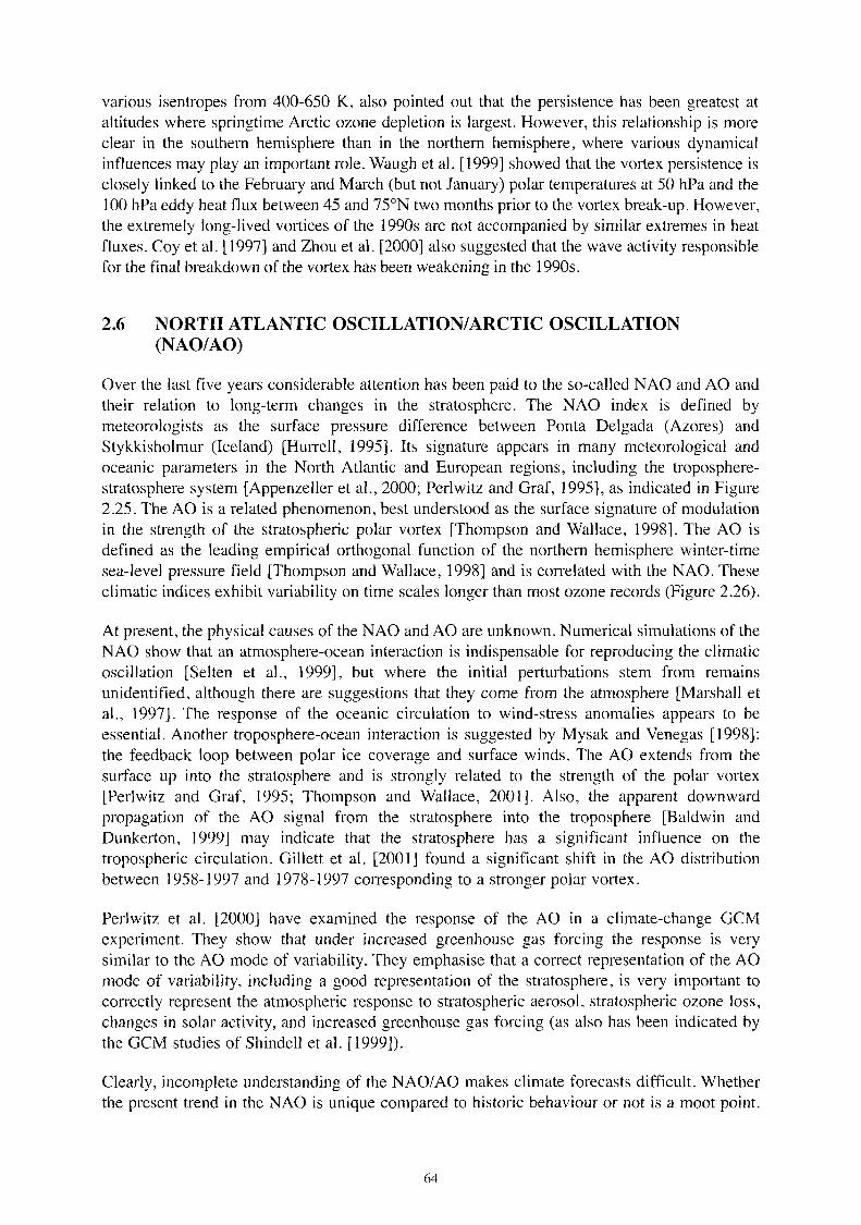
various isentropes from 400-650 K, also pointed out that the persistence has been greatest at altitudes where springtime Arctic ozone depletion is largest. However, this relationship is more clear in the southern hemisphere than in the northern hemisphere, where various dynamical influences may play an important role. Waugh et al. [1999) showed that the vortex persistence is closely linked to the February and March (but not January) polar temperatures at 50 hPa and the 100 hPa eddy heat flux between 45 and 75°N two months prior to the vortex break-up. However, the extremely long-lived vortices of the 1990s are not accompanied by similar extremes in heat fluxes. Coy et al. [ 1997) and Zhou et al. [2000) also suggested that the wave activity responsible for the final breakdown of the vortex has been weakening in the 1990s.

2.6 NORTH ATLANTIC OSCILLATION/ARCTIC OSCILLATION (NAO/AO)

Over the last five years considerable attention has been paid to the so-called NAO and AO and their relation to long-term changes in the stratosphere. The NAO index is defined by meteorologists as the surface pressure difference between Ponta Delgada (Azores) and Stykkisholmur (Iceland) [Hurrell, 1995). Its signature appears in man y meteorological and oceanic parameters in the North Atlantic and European regions, including the troposphere­stratosphere system [Appenzeller et al., 2000; Perlwitz and Graf, 1995), as indicated in Figure 2.25. The AO is a related phenomenon, best understood as the surface signature of modulation in the strength of the stratospheric polar vortex [Thompson and Wallace, 1998). The AO is defined as the leading empirical orthogonal fonction of the northern hemisphere winter-time sea-level pressure field [Thompson and Wallace, 1998) and is conelated with the NAO. These climatic indices exhibit variability on time scales longer than most ozone records (Figure 2.26).

At present, the physical causes of the NAO and AO are unknown. Numerical simulations of the NAO show that an atmosphere-ocean interaction is indispensable for reproducing the climatic oscillation [Selten et al., 1999), but where the initial perturbations stem from remains unidentified, although there are suggestions that they corne from the atmosphere [Marshall et al., 1997). The response of the oceanic circulation to wind-stress anomalies appears to be essential. Another troposphere-ocean interaction is suggested by Mysak and Venegas [ 1998): the feedback loop between polar ice coverage and surface winds. The AO extends from the surface up into the stratosphere and is strongly related to the strength of the polar vortex [Perlwitz and Graf, 1995; Thompson and Wallace, 2001). Also, the apparent downward propagation of the AO signal from the stratosphere into the troposphere [Baldwin and Dunkerton, 1999) may indicate that the stratosphere has a significant influence on the tropospheric circulation. Gillett et al. [2001] found a significant shift in the AO distribution between 1958-1997 and 1978-1997 conesponding to a stronger polar vortex.

Perlwitz et al. [2000) have examined the response of the AO in a climate-change GCM experiment. They show that under increased greenhouse gas forcing the response is very similar to the AO mode of variability. They emphasise that a conect representation of the AO mode of variability, including a good representation of the stratosphere, is very important to conectly represent the atmospheric response to stratospheric aerosol, stratospheric ozone loss, changes in solar activity, and increased greenhouse gas forcing (as also has been indicated by the GCM studies of Shindell et al. [ 1999]).

Clearly, incomplete understanding of the NAO/AO makes climate forecasts difficult. Whether the present trend in the NAO is unique compared to historie behaviour or not is a moot point.

64

80°N

60°N -

4 0°N -

20°N -

■

oo -~---~----- ~------------~------~~ 100°W 60°w 20°w 20°E

-1.0 -0.5 0.0 0.5 1.0

Figure 2.25 Cross corre!ation map (in colours) between winter mean (December-March) tropopause pressure and NA O index both derived fro m NCEP reanalysis da/a fo r the period 1958 to 1998 . On/y correlation coefficients abovelbelow ±0.3 are shown . Contours indicate tropopause pressure variation (in hPa) associatecl with + l a in NA O index, (A) location ofArosa and (R) location of Reykjavik. [Appenzel/er et al ., 2000.]

X (l)

~ 4

1 2 0 <(

z 0

1875 1900 _J_

1925 1950 1975 2000

Year

Figure 2.26 No rma!ised time series of NA O index f or winters (Dece111ber-March) .fim n 1864 to the present , basecl on da ta fro m Hurre/1 (http://wwiv.met .rdg.ac .uk/cag!NA O!index.html)

65

There have been many attempts to reconstruct the climate and the NAO of the past, employing historical weather records, tree ring data and ice core data [Appenzeller et al., 1998, and references therein]. Less work has been done with the AO, as it requires the pressure field of the whole hemisphere. There have been suggestions that the observed NAO/ AO variation is a random or chaotic behaviour, which does not depend on external forcing [Christiansen, 2001; Stephenson et al., 2000]. This would mean that the observed NAO/AO long-term behaviour is natural variability. The other possibility implies an anthropogenic influence, i.e., that the cun-ently observed NAO and AO change is a response to anthropogenic climate forcing [Hoerling et al., 200 l; Paeth et al., 1999; Shindell et al., 1999].

2.7 CHANGES IN STRATOSPHERIC AEROSOLS SINCE THE 1970S.

The lower stratosphere, between the tropopause and about 30 km, contains a layer of aerosol pai1icles, composed mainly of spherical droplets of sulphuric acid solution. Under background conditions (such as have pertained since 1996) the monomodal droplet size distribution peaks at radii of 50-80 nm and the aerosol layer often extends only to 25-27 km. Following a major volcanic eruption however, the total number of particles increases (up to a hundredfold), a population of larger particles (radii ~200-300 nm) is formed, and the layer extends above 30 km. Aerosol is important for a full understanding of the ozone layer for two reasons:

a) heterogeneous chemical reactions take place on aerosol surfaces - primarily conversion of N20 5 to HN03 but also, at temperatures <200 K, conversion of halogen reservoirs to free radicals.

b) aerosol affects radiative transfer in the stratosphere and thus impacts the dynamics (Section 2.5.1).

We present in this section the longest record of stratospheric aerosol measurements that exist in Europe- the lidar record at Garmisch-Partenkirchen (47.5°N, ll.1°E), which began in 1976 and which bas been part of the NDSC since 1991. The lidar provides measurements of particle backscatter with high ve11ical resolution. A conversion model is used to calculate aerosol extinction, mass and surface from the backscatter data. This model is based on height and time­resolved aerosol size distributions derived from balloon-borne particle counter data from Laramie, Wyoming [Jager and Hofmann, 1991; Jager et al., 1995].

The lidar record of Figure 2.27 shows the integrated particle backscatter coefficient at 694.3 nm. Data are integrated from l km above the tropopause to the top of the aerosol layer at 30-35 km. The measurement density is several soundings per month. Volcanic eruptions of various magnitudes have been observed at this northern mid-latitude site: perturbations of global and long lasting significance (years) were caused by the equatorial eruptions of El Chichon (Mexico, 1982) and Pinatubo (Philippines, 199 l), and hemispheric perturbations ( of about l year) by the high latitude eruptions of St. Helens (USA, 1980) and Alaid (Kurile Islands, 1981 ). Other tropical eruptions causing diffuse backscatter increases were La Soufriere (Caribbean, 1979), Sie1Ta Negra (Galapagos, 1979), Nyamuragira (Zaire, the "Mystery Cloud'' of 1981), Nevada del Ruiz (Colombia, 1985) and Nyamuragira (Zaïre, 1986), the latter two probably delaying the decay of the El Chichon perturbation. A fm1her category is high latitude eruptions of only local significance which had no lasting effect on the lidar record but could be traced in individual backscatter profiles: Redoubt (Alaska, 1989), Kliuchevskoi (Kamchatka, 1994), and finally Shishaldin (Aleu tian Islands, 1999).

66

IFU GARMISCH-PARTENKIRCHEN 47.5°N, 11.1°E

w 10-2 -=-----------------------------------.=-d TROPOPAUSE+ 1 km TO LAYER TOP ~ ,._ 0::: .!!:., <r: o::: 10-3

Cl. w 0 ~ w <(

~ u 10-4 0::: (j)

(.? ès w <( !z CO 10-5 -+-----.--,---r'-_.,........_,....._-+'----r----ir--~.....,_ ........... _-,----,---+-T'"'""'"--.----.--.------r----,--,-----.'--+-

76 77 78 79 80 81 82 83 84 85 86 87 88 89 90 91 92 93 94 95 96 97 98 99

YEAR

Figure 2.27 Tilne variation of the integrated aerosol backscatter from lidar measurements of the stratospheric aerosol layer at northern hemisphere mid-latitudes. The dashed line indicates the 1979 mean. Volcanic eruptions are marked.

This record of stratospheric particle load, which is typical for northem mid-latitudes, is characterised by two periods of increased volcanism and by three periods with little or no influence by volcanic eruptions, namely 1977 to 1979, 1989 to 1991, and 1997 up to the present time. The decay of the Pinatubo aerosol load terminated in 1996 when the 1979 background level was reached. In the background period prior to the Pinatubo eruption, however, a decay to values comparable with the late 1970s or 1990s could not be observed. Then Hofmann [ 1991] and Jager [ 1994] discussed the possibility of anthropogenic influences contaminating the lower stratosphere. The retum of the stratospheric aerosol load after the decay of the Pinatubo perturbation to values around the 1979 minimum indicates that any anthropogenic contribution to stratospheric aerosol must be far less than estimated in the previous EC assessment.

67