Long-term correction of wind measurements State-of-the-art, guidelines and future work

Elforsk report 13:18

Sónia Liléo, Erik Berge, Ove Undheim, Rickard Klinkert and Rolv E. Bredesen, Kjeller Vindteknikk, January 2013

Long-term correction of wind measurements State-of-the-art, guidelines and future work

Elforsk report 13:18

Sónia Liléo, Erik Berge, Ove Undheim, Rickard Klinkert and Rolv E. Bredesen, Kjeller Vindteknikk, January 2013

ELFORSK

Preface The description of the temporal variability of the wind conditions is essential when assessing the wind conditions at sites potentially suitable to wind power development. In order to describe the effects of the use of different long-term datasets, as well as the effects of the use of different long term correction methods, project V-377, Long-term correction of wind measurements, was carried out within the Swedish wind energy research program "Vindforsk - III".

The work was carried out by Kjeller Vindteknikk with Sónia Liléo as project leader. This report is the final report of the project.

Apart from funding from Vindforsk, Kjeller Vindteknikk has also contributed to the funding of the project.

Vindforsk - III is funded by ABB, Arise windpower, AQSystem, E.ON Elnät, E. ON Vind Sverige, Energi Norge, Falkenberg Energi, Fortum, Fred. Olsen Renewables, Gothia wind, Göteborg Energi, Jämtkraft, Karlstads Energi, Luleå Energi, Mälarenergi, O2 Vindkompaniet, Rabbalshede Kraft, Skellefteå Kraft, Statkraft, Stena Renewable, Svenska Kraftnät, Tekniska Verken i Linköping, Triventus, Wallenstam, Varberg Energi, Vattenfall Vindkraft, Vestas Northern Europe, Öresundskraft and the Swedish Energy Agency.

Comments on the work and the final report have been given by a reference group composed by the following members: Lasse Johansson from AQSystem, Johannes Lundvall from Stena Renewable, Måns Håkansson from Statkraft, Morten Thøgersen from EMD International, and Lars Landberg from GL Garrad Hassan.

Stockholm January 2013

Anders Björck

Programme maganger Vindforsk-III

Electricity- and heatproduction, Elforsk

ELFORSK

Acknowledgements by the authors The authors would like to thank the Vindforsk - III research programme for co-funding this project, and the members of the reference group, Lasse Johansson, Johannes Lundvall, Måns Håkansson, Morten Thøgersen, and Lars Landberg, for valuable comments on the work. Furthermore, the authors are also thankful to the colleagues Knut Harstveit, Øyvind Byrkjedal and Lars Tallhaug at Kjeller Vindteknikk for valuable discussions.

The authors thank EMD Internatial AS for providing a temporary license of the WindPRO's MCP module, and GL Garrad Hassan for providing a temporary license of the software WindFarmer.

Finally, the authors also want to acknowledge the entities listed below for their work in producing the different long-term datasets used in this study, and for providing public access to these data.

NCEP/NCAR for the development of the R1 reanalysis project.

NOAA/OAR/ESRL PSD, Boulder, Colorado, USA, for providing NCEP Reanalysis derived data via their webpage (PSD, 2012).

The Japan Meteorological Agency (JMA) and the Central Research Institute of Electric Power Industry (CRIEPI) for the development of the JRA-25 long-term reanalysis cooperative research project.

ECMWF for the development of the ERA-Interim reanalysis project.

Global Modeling and Assimilation Office (GMAO) and the GES DISC (Goddard Earth Sciences Data and Information Services Center) for the dissemination of MERRA.

NCEP for the development of the CFSR reanalysis project and for the production of CFSv2 data.

The U.S. Department of Energy, Office of Science Innovative and Novel Computational Impact on Theory and Experiment (DOE INCITE) program, Office of Biological and Environmental Research (BER), and the National Oceanic and Atmospheric Administration Climate Program Office for providing support to the Twentieth Century Reanalysis Project (20CR).

The Research Data Archive (RDA) which is maintained by the Computational and Information Systems Laboratory (CISL) at the National Center for Atmospheric Research (NCAR) for providing data access via their webpage (RDA, 2012) to a large number of datasets. NCAR is sponsored by the National Science Foundation (NSF). The CFSR, CFSv2 and 20CRv2 datasets used in this study were retrieved from RDA (2012).

ELFORSK

Summary The main purposes of this study are to report on the state-of-the-art long-term datasets available for use in the long-term correction of wind measurements, as well as on the long-term correction methods most commonly used at the present; to present guidelines on how to reduce the uncertainty in the long-term correction of wind measurements; to give recommendations on the expected intervals of the uncertainty associated with different contributing factors, and finally, to highlight issues in need of further investigation.

A description of the main properties of different long-term datasets is given in Chapter 2. These are categorized into long-term weather observations, reanalysis global datasets, and reanalysis mesoscale datasets. The ability of these long-term datasets to describe the local wind climate in terrain with low complexity is discussed in Chapter 3. The results indicate that the reanalysis global dataset MERRA, as well as the reanalysis mesoscale datasets WRF FNL and WRF ERA-Interim, are, among the selected datasets, the most suitable to the use in the long-term correction of wind measurements performed in terrain with low complexity. The results also suggest that the increase of the spatial resolution of a long-term dataset to finer than about 0.5 x 0.5 degrees in latitude and longitude (~55 km x 30 km in Scandinavia) does not necessarily result in the increase of the hourly correlation coefficient of its relationship to site wind measurements. Note that the above conclusions are based on our best judgement of the obtained results, and not on the comparison with a known answer. The analysis of the monthly correlation coefficients shows only small differences between the selected reference datasets. A discussion is conducted on the need of a more appropriate measure of the long-term data's representativeness, i.e., of how well a long-term data series from a given position represents the long-term wind variations at another position. Neither the hourly nor the monthly correlation coefficients represent an ideal measure of the long-term data's representativeness.

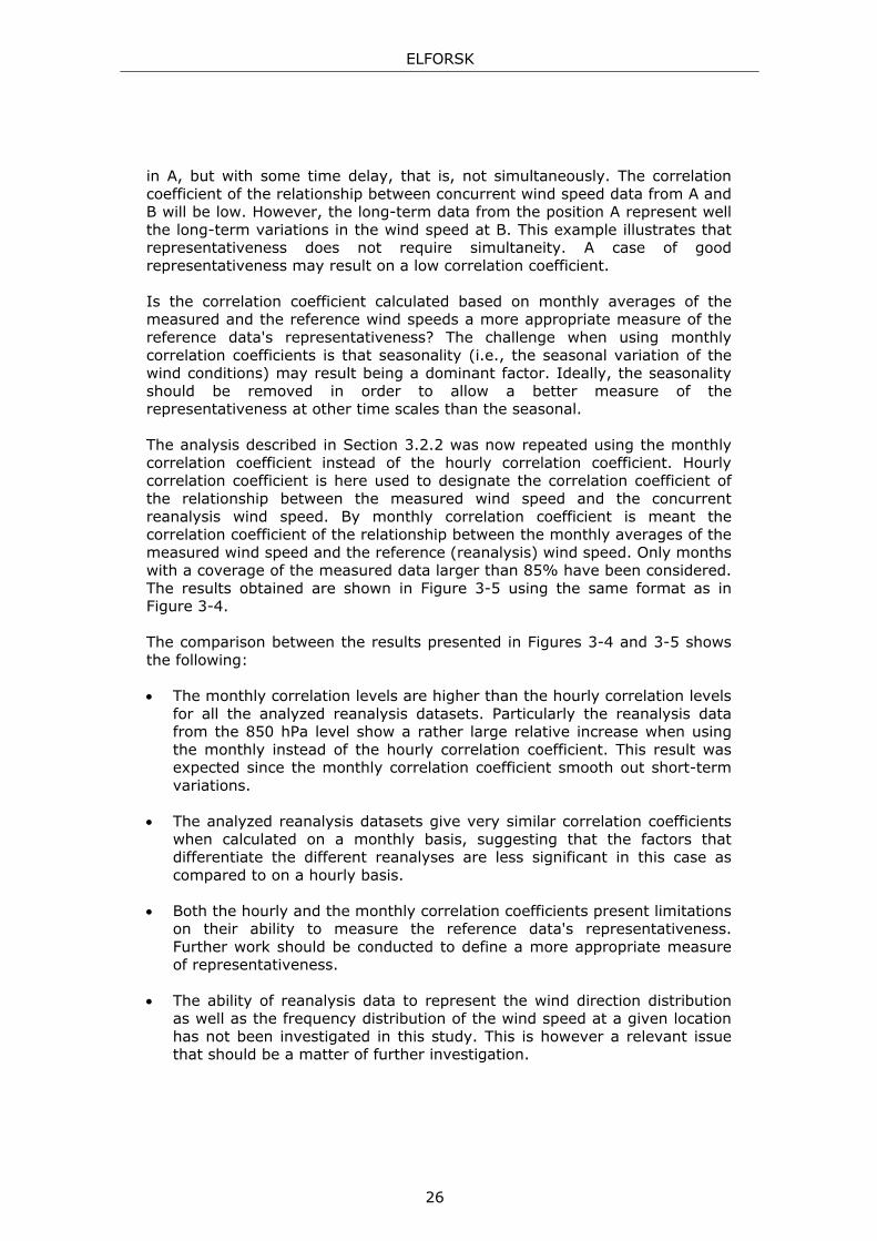
In addition to the uncertainty arising from the long-term correction process, the uncertainty related to the inter-annual variability of the wind speed is also relevant. This issue is discussed in Chapter 4. The results show that the inter-annual variability of the wind speed is rather site specific, and should therefore be evaluated specifically for the site in consideration. Values ranging between 3 and 7 % are found in the analyzed region (Norway, Denmark, Sweden, Finland and the Baltic countries), based on reanalysis data.

Since the future long-term wind conditions are unknown, it is assumed that the past may be used as a predictor of the future wind conditions. A given time period of the past is chosen (reference period), and the wind conditions observed in this period are considered representative of the future wind conditions. The variations observed in the past wind climate are discussed in Chapter 5, based on wind speed data from the reanalysis dataset 20CRv2. In an earlier study by Wern and Bärring (2009), an average negative long-term trend (-4%) was found in the wind speed in Sweden for the period 1951 to 2008. The authors emphasized though that this trend was not statistically significant. The results presented here confirm that there is no statistically significant trend in the wind speed during that period in Sweden. However, the wind speed over central and northern Norway shows a positive long-term

ELFORSK

trend (2-3 %) in the period 1951-2008 that is statistically significant. The analysis of the past wind climate has also led to the conclusion that the period 1989 to 1995 was characterized by unusual high annual mean wind speeds associated with a large positive peak in the North Atlantic Oscillation (NAO) index. The decrease in the mean wind speed seen between 1990 and 2005 represents a return to the longer-term mean, after the unusually large maximum in 1990.

Chapter 6 discusses the assumption of the past being used as a predictor of the future wind conditions. The performed analysis shows that the prediction error associated with this assumption is about 1.5 - 2 %, but may vary up to 6 % in a worst-case scenario. Random and consecutive sampling of the years forming the reference period has been tested. Consecutive sampling resulted in a slightly smaller prediction error as compared to random sampling. This result suggests the existence of a weak underlying pattern (non-randomness) in the annual mean wind speed from one year to the next. Another relevant issue is the optimal length of the reference period that minimizes the prediction error. That is, how long should the long-term reference period be? The results show a significant decrease of the mean prediction error with the increase of the reference period length from 1 to about 12-15 years, remaining in average rather constant (1.5 %) for longer reference periods. The standard deviation from the mean value shows however a slight increase for lengths larger than 20 years. Based on these results, the choice of a reference period length of about 15 to 20 years is recommendable. The choice of a 15 to 20-year long reference period from the near past period 1993-2012 gives multiple alternatives: the 17-year period 1996-2012 as an example of a more conservative choice; and the 20-year period 1993-2012 as a less conservative choice.

A categorization of the most commonly used long-term correction methods, into regression and non-regression methods, is presented in Chapter 7. A description of the main properties of these methods is given. Furthermore, the self-prediction ability of these methods is analyzed. The results show an average prediction error of about 1.5 to 2 %, and a normal variation up to 4 %, independently on the method applied, provided that the hourly correlation between reference and measured data is larger than 75-80 %. The performance of the methods has not been analyzed for cases with lower correlation coefficients.

Based on the results summarized above, guidelines have been defined in Chapter 9 on the evaluation of the uncertainty associated with the long-term correction of wind measurements, and of the uncertainty associated with the inter-annual variability of the wind speed. Expected uncertainty intervals are presented for the different sources contributing to the total uncertainty. The assumption of using the past as a predictor of the future wind climate is seen to contribute significantly to the total uncertainty in the long-term corrected wind speed. The increase of the measurement period from 1 year (with a coverage of the quality controlled data larger than 85 %) to 2 years, is shown to reduce the uncertainty in the long-term corrected wind speed from 2.1-4.5 % to about 1.8-3.6 %. The largest reduction is seen when increasing the measurement period length from some months to one complete year.

Finally, several issues in need of further investigation are highlighted in Chapter 10.

ELFORSK

Sammanfattning Huvudmålen med denna studie är att presentera olika långtidsdataserier som kan användas vid normalårskorrigering av vindmätningar, med speciell fokus på de senast utvecklade serierna; beskriva de vanligaste normalårskorrigeringsmetoderna; presentera riktlinjer för hur osäkerheten i normalårskorrigering kan reduceras; ge rekommendationer om osäkerhetens förväntade intervall för olika bidragande faktorer och, slutligen, att definiera frågor som är i behov av framtida forskning och utvecklingsarbete.

En beskrivning av huvudegenskaperna hos olika långtidsdataserier ges i kapitel 2. Dessa serier är grupperade enligt tre kategorier: långtidsväderobservationer, globala reanalysdataserier och mesoskaliga reanalysdataserier. De olika långtidsdataseriernas förmåga att beskriva det lokala vindklimatet i terräng med låg komplexitet diskuteras därefter i kapitel 3. Resultaten visar att, av de analyserade serierna, är den globala reanalysdataserien MERRA och de mesoskaliga dataserierna WRF FNL och WRF ERA-Interim, de som lämpar sig bäst för normalårskorrigering av vindmätningar utförda i terräng med låg komplexitet. Resultaten indikerar även att ökningen av en dataseries rumsupplösning till mer än cirka 0.5 x 0.5 grader i latitud och longitud (~55 km x 30 km i Skandinavien) inte nödvändigtvis resulterar i en ökning av korrelationskoefficienten med vindmätningar utförda i terräng med låg komplexitet. Notera att dessa slutsatser baserar sig på vår bästa bedömning av de erhållna resultaten, och inte på en jämförelse mot ett känt svar. Analysen av korrelationskoefficienten baserad på månadsmedelvärdena av serierna visar endast små skillnader mellan de analyserade dataserierna. Behovet av ett mer korrekt mått på långtidsdatats representativitet, det vill säga hur bra långtidsdata från en given position representerar vindens långtidsvariationer i en annan position, har diskuterats. Varken korrelationskoefficienten beräknad med timmesdata eller med månadsdata är ett idealt mått på långtidsdatas representativitet.

Förutom att ta hänsyn till osäkerheten som resulterar från normalårskorrigeringsprocessen är det även relevant att ta hänsyn till osäkerheten relaterad till vindens årliga variabilitet. Denna fråga är analyserad i kapitel 4. Resultaten antyder att den årliga variationen av vindhastigheten är platsspecifik och bör därför estimeras individuellt för det aktuella området. Vindens årliga variabilitet beräknad baserad på reanalysdata varierar mellan 3 och 7 % i det analyserade området (Norge, Danmark, Sverige, Finland och Baltikum).

Eftersom de framtida långtidsvindförhållandena är okända antas det att det förgångna kan användas för att förutsäga det framtida vindklimatet. En viss tidsperiod från det förgångna väljs (referensperiod) och vindförhållandena observerade under denna period anses vara representativa för de framtida vindförhållandena. Det förgångna vindklimatet analyseras i kapitel 5 utifrån vindhastighetsdata från den globala reanalysdataserien 20CRv2. I en tidigare studie utförd av Wern och Bärring (2009) har en negativ trend (-4 %) estimerats för vindhastigheten i Sverige under perioden 1951-2008. Wern och Bärring betonade dock att denna trend inte anses vara statistiskt signifikant. Resultaten som presenteras i denna rapport bekräftar att det inte finns någon statistiskt signifikant trend i vindhastigheten under denna period i Sverige. Resultaten visar däremot en positiv trend (2-3 %) som är statistiskt

ELFORSK

signifikant i vindhastigheten under 1951-2008 för centrala och norra Norge. Analysen av det förgångna vindklimatet har även lett till slutsatsen att den årliga medelvinden var ovanlig hög under perioden 1989 till 1995, associerad med en hög topp i NAO indexet (NordAtlantiska Oscillationen). Minskningen i den genomsnittliga vindhastigheten sett mellan 1990 och 2005 representerar en återgång till vindens långtidsmedelvärde, efter det ovanligt stora maximum det haft år 1990.

I kapitel 6 presenteras en diskussion kring antagandet att det förflutna kan användas för att prediktera det framtida vindklimatet. Den genomförda analysen visar att prediktionsfelet som resulterar från detta antagande är cirka 1.5 - 2 %, men kan variera upp till ett maximum av 6 %. Slumpmässigt och konsekutivt urval av de åren som bygger referensperioden har testats. Konsekutivt urval resulterade i ett något mindre prediktionsfel jämfört med slumpmässigt urval. Detta resultat tyder på förekomsten av ett svagt underliggande mönster (icke-slumpmässighet) i den årliga medelvinden från år till år. En ytterligare relevant fråga är den optimala längden av referensperioden som minimerar prediktionsfelet. Det vill säga, hur lång ska referensperioden vara? Resultaten visar en signifikant minskning av det genomsnittliga prediktionsfelet när referensperiodens längd ökas från 1 till cirka 12-15 år och ett relativt konstant prediktionsfel (1.5%) för längre referensperioder. Standardavvikelsen från medelvärdet visar dock en svag ökning för perioder längre än 20 år. Baserad på dessa resultat, vi rekommenderar valet av en referensperiod som är 15 till 20 år lång. Valet av en 15 till 20 år lång referensperiod från den senaste 20-årsperioden (1993-2012) ger olika alternativ: den 17 år långa perioden 1996-2012 som ett exempel på ett mer konservativt val; och den 20 år långa perioden 1993-2012 som ett mindre konservativt val.

En kategorisering av de vanligaste normalårskorrigeringsmetoderna i regressions- och icke-regressionsmetoder presenteras i kapitel 7. Huvudegenskaperna hos dessa metoder beskrivs och deras självprediktionsförmåga analyseras. Resultaten visar ett genomsnittligt prediktionsfel på cirka 1.5 till 2 % och en normal variation upp till 4 %, oberoende av den använda metoden. Detta förutsatt att en korrelationskoefficient (R) mellan referens och uppmätt timmesdata är högre än 75-80 %.

Utifrån de ovannämnda resultaten presenteras riktlinjer i kapitel 9 rörande estimering av osäkerheten associerad med normalårskorrigering och osäkerheten associerad med vindens årliga variabilitet. Förväntade intervall för de olika bidragande osäkerhetskällorna definieras. Antagandet att det förgångna kan användas för att prediktera det framtida vindklimatet är en starkt bidragande orsak till den totala osäkerheten i den normalårskorrigerade vindhastigheten. Ökningen av mätperiodens längd från 1 år (där täckningen av det kvalitetskontrollerade datat är högre än 85 %) till 2 år minskar den totala osäkerheten i den normalårskorrigerade vindhastigheten från 2.1-4.5 % till cirka 1.8-3.6 %. Den största minskningen av osäkerheten sker vid ökandet av mätperiodens längd från några månader till ett helt år.

Slutligen, presenteras i kapitel 10 frågor i behov av framtida forskning och utvecklingsarbete.

ELFORSK

Contents

1  Introduction 1 

2  Description of different long-term reference datasets 4 2.1  Long-term weather observations ....................................................... 4 

2.1.1  NCEP ADP Global Surface Observations ................................... 4 2.1.2  Satellite observations of the ocean surface ............................... 6 

2.2  Reanalysis global datasets ................................................................ 7 2.2.1  NCEP/NCAR Reanalysis 1 ....................................................... 8 2.2.2  NCEP/DOE Reanalysis 2 ........................................................ 9 2.2.3  NCEP/CFSR and NCEP/CFSv2 ................................................. 9 2.2.4  NOAA-CIRES Twentieth Century Global Reanalysis Version II

(20CRv2). ......................................................................... 10 2.2.5  MERRA ............................................................................. 10 2.2.6  ERA-Interim and ERA-40 ..................................................... 11 2.2.7  JRA-25 and JRA-55 ............................................................. 11 2.2.8  Summary of the main properties of different reanalysis global

datasets............................................................................ 12 2.3  Reanalysis mesoscale datasets ........................................................ 14 

2.3.1  WRF FNL ........................................................................... 14 2.3.2  WRF ERA-Interim ............................................................... 15 

3  Using reanalysis data to describe the local wind climate in terrain with low complexity 16 3.1  Analysis of the temporal and spatial characteristics of reanalysis data ... 16 

3.1.1  Linear rate of change maps ................................................. 17 3.1.2  Decomposition into high and low-frequency components .......... 21 

3.2  Strength of the relationship to local wind measurements ..................... 23 3.2.1  Description of the database used .......................................... 23 3.2.2  Results ............................................................................. 23 3.2.3  Is the correlation coefficient an appropriate measure of

representativeness? ............................................................ 25 

4  Inter-annual variability of the wind speed 28 

5  The past wind climate according to 20CRv2 data 31 5.1  Statistically significant long-term trends in the wind speed .................. 31 5.2  Relation between the wind variations and the North Atlantic Oscillation . 36 

6  Choice of the reference period 39 6.1  Accuracy in the assumption of the past being a predictor of the future

wind conditions ............................................................................. 39 6.2  Random and consecutive sampling ................................................... 42 6.3  Dependence of the prediction error on the reference period length ....... 44 

7  Long-term correction methods 49 7.1  Description of different LTC methods ................................................ 50 

7.1.1  Regression LTC methods ..................................................... 50 7.1.2  Non-regression LTC methods ............................................... 53 

7.2  Uncertainty associated with the different LTC methods ........................ 58 7.3  Dependence of the prediction error on the measurement period length . 62 

8  Conclusions 67 

ELFORSK

9  Guidelines on uncertainty reduction and on expected values for the uncertainty interval 71 

10  Future work 75 

11  Appendix - U&N method 76 11.1  Method description ........................................................................ 76 

11.1.1  Long-term direction distribution ........................................... 76 11.1.2  Long-term wind speed distribution ........................................ 77 

12  Bibliography 80 

ELFORSK

1

1 Introduction

The description of the temporal variability of the wind conditions is essential when assessing the wind conditions at sites potentially suitable to wind power development. Wind measurements are typically performed during a relatively short time period (~1-3 years), that is commonly not representative of the long-term wind conditions at the site. Long-term correction of the wind measurements is therefore needed in order to estimate the expected long-term wind climate that best represents the site. Figure 1-1 illustrates the main steps involved in the long-term correction of wind measurements. The bulleted items indicate relevant factors that should be taken into account in the assessment of the uncertainty in the estimated long-term wind climate.

Figure 1-1. Schematic illustration of the process involved in the long-term correction of wind measurements. The bulleted items indicate parameters of high relevance for the estimate of the uncertainty in the resultant long-term corrected wind climate.

1. Short-term site measurements Accuracy of the measurements Measurements'

representativeness of the long-term site wind climate

2. Long-term reference data Characteristics of the data Data's representativeness of the

long-term site wind climate

3. Long-term correction methodology Self-prediction ability

4. Past as predictor of the future Assumption accuracy Length of the past period

5. Estimate of the long-term wind climate at the measurement site and corresponding uncertainty

ELFORSK

2

The two main elements given as input to the long-term correction process are the wind measurements performed at the site under a given time period (short-term period), and the long-term data from a representative location. How well the short-term data represent the wind farm's long-term wind climate is mainly determined by the quality of the measurements and by the measurement period length (box 1 in Figure 1-1). This is often about 1 year, in order to capture the seasonal variations of the meteorological conditions. However, the longer-term variability of the wind conditions is not captured. It is therefore necessary to find a long-term time series that is believed to represent appropriately the long-term wind climate at the measurement site. The long-term data's representativeness is an important factor that should be evaluated, as well as the characteristics of the data (box 2 in Figure 1-1). By representativeness it is meant how well the chosen long-term data represent the long-term variations of the wind conditions at the measurement site. The long-term data shall be representative, i.e, shall describe in an appropriate way the long-term variations of the wind conditions at the measurement site. Furthermore, the long-term data shall describe real changes in the local climatic conditions, and shall not be affected by artificial changes caused by modifications in the measurement system or in the methodology used in the generation of the data. For this reason, the analysis of the spatial and temporal characteristics of the long-term data is essential. When the short-term and the long-term data series have been established, a long-term correction methodology is applied with the main purpose of obtaining an adequate description of the long-term wind climate at the measurement site. The accuracy of the used long-term correction method is dictated by its self-prediction ability, i.e., its ability to predict a known answer (box 3). The future wind climate is however unknown. It is therefore assumed that the past is as a predictor of the future wind climate, i.e., the statistical properties of the future wind climate are assumed to be the same as for the past wind climate. The accuracy of this assumption is however of major importance for the accuracy of the estimated long-term site wind conditions and shall therefore be evaluated Moreover, one has to define how long is the future period for which the energy production should be calculated, and how long back in time should one look at in order to predict the wind conditions in the future period of interest (box 4 in Figure 1-1). Adopting the investor's perspective, the length of future period of interest is equal to the length of the amortization period. The investor needs to know how much energy a wind farm is expected to produce during the period the debt has to be paid off (amortization period). This is typically 10 to 20 years. In cases when no debts have to be paid, the future period of interest is the lifetime of the wind farm, when the profits will be collected. This is typically 20 years. For these reasons, the energy production of a wind farm is often estimated for a long-term period of 10 to 20 years. The question that follows is, how long back in the past the long-term reference data shall extend in order to accurately predict the wind conditions in the future 10 to 20 years.

ELFORSK

3

The main goals of this investigation study are to provide a description of the state-of-the-art long-term datasets and correction methods that may be used in the long-term correction of wind measurements; to obtain fundamental results that aid the definition of guidelines on how to more accurately long-term correct wind measurements, and on how to assess the uncertainty in the estimated result; and finally, to highlight relevant issues in need of further investigation. This report is structured as follows. Chapter 2 gives a description of the main properties of different long-term datasets. The ability of these datasets to describe the local wind climate in terrain with low complexity is discussed in Chapter 3. Besides the contribution of the uncertainty arising from the long-term correction process, the uncertainty related to the inter-annual variability of the wind speed should also be considered. This issue is discussed in Chapter 4. The variations observed in the past wind climate are discussed in Chapter 5, and the uncertainty in the assumption of the past being a predictor of the future wind conditions, as well as in the choice of the reference period length, is investigated in Chapter 6. Chapter 7 begins with a description of different long-term correction models typically used in industry at the present. This is followed by an analysis on the accuracy of these models, and on the influence of the measurement period length. A summary of the main conclusions obtained in this investigation study is presented in Chapter 8. Based on these conclusions, guidelines on the assessment of the uncertainty resultant from the long-term correction process are defined in Chapter 9. Several issues have been identified during the development of this project considered of relevance for further investigation. These are highlighted in Chapter 10.

ELFORSK

4

2 Description of different long-term reference datasets

There are several types of long-term reference datasets. These may be wind measurements from weather stations or from satellites, reanalysis global datasets or reanalysis mesoscale datasets. This chapter distinguishes between these different types of long-term reference datasets, and gives a description of the most relevant ones.

2.1 Long-term weather observations

In-situ observations from climate monitoring stations operated by national weather institutions constitute a valuable source of measurements of several atmospheric parameters such as temperature, barometric pressure, humidity, wind speed, wind direction, and precipitation. These data are mainly used in climate monitoring, weather forecasting, severe weather warnings and for research purposes. They may however also be used as reference data for use in wind resource assessment if the datasets cover a sufficient long time period.

2.1.1 NCEP ADP Global Surface Observations

The NCEP ADP dataset includes observations from land surface stations and from marine platforms that are collected by the National Centers for Environmental Prediction (NCEP) using the coordinated global system of telecommunications known as GTS. The collected GTS reports are decoded by NCEP using Automated Data Processing (ADP) and stored in files with a synoptic time stamp. The term "synoptic surface observations" refers to observations made near the surface simultaneously on different weather stations located all over the globe.

The NCEP ADP observations from land surface stations include SYNOP and METAR weather reports, as well as AWOS and ASOS report types. The SYNOP reporting code is generally used to report observations made at manned and automated weather stations, while the METAR format is typically used in weather reports made at airports and military bases. SYNOP reports are typically generated every six hours, while METAR reports are normally sent once an hour. The reporting frequency may however differ between stations. Weather reports generated by airport weather stations located in the United States are generally designated by AWOS (Automated Weather Observing System) and ASOS (Automated Surface Observing System) reports. The main difference between these systems is related to which institutions are responsible for the operation and control of the units.

ELFORSK

5

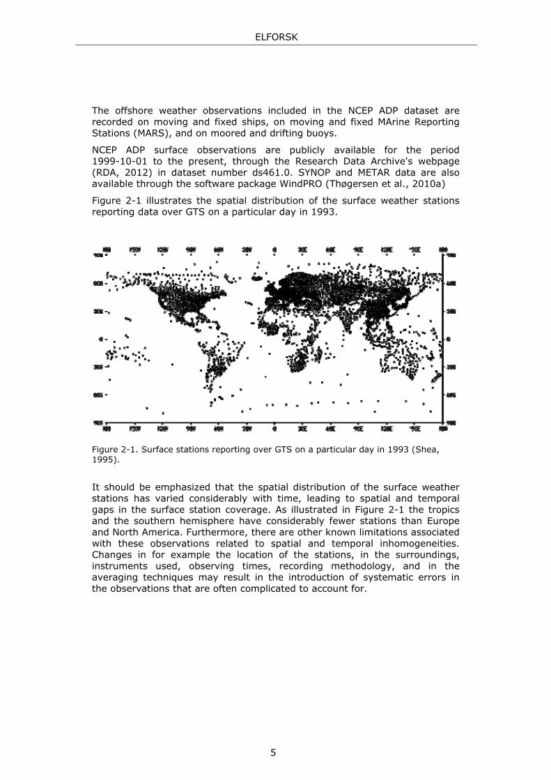
The offshore weather observations included in the NCEP ADP dataset are recorded on moving and fixed ships, on moving and fixed MArine Reporting Stations (MARS), and on moored and drifting buoys.

NCEP ADP surface observations are publicly available for the period 1999-10-01 to the present, through the Research Data Archive's webpage (RDA, 2012) in dataset number ds461.0. SYNOP and METAR data are also available through the software package WindPRO (Thøgersen et al., 2010a)

Figure 2-1 illustrates the spatial distribution of the surface weather stations reporting data over GTS on a particular day in 1993.

Figure 2-1. Surface stations reporting over GTS on a particular day in 1993 (Shea, 1995).

It should be emphasized that the spatial distribution of the surface weather stations has varied considerably with time, leading to spatial and temporal gaps in the surface station coverage. As illustrated in Figure 2-1 the tropics and the southern hemisphere have considerably fewer stations than Europe and North America. Furthermore, there are other known limitations associated with these observations related to spatial and temporal inhomogeneities. Changes in for example the location of the stations, in the surroundings, instruments used, observing times, recording methodology, and in the averaging techniques may result in the introduction of systematic errors in the observations that are often complicated to account for.

ELFORSK

6

2.1.2 Satellite observations of the ocean surface

QuikSCAT and Seawinds data

QuikSCAT is the name of a satellite launched on 1999 carrying onboard a microwave scatterometer named SeaWinds. As the name suggests, the main mission of this scatterometer was to measure the wind near the ocean surface. The QuikSCAT satellite was operational until the end of 2009. At the end of 2002, a nearly identical SeaWinds scatterometer was launched onboard the satellite ADEOS-II which though failed about 1 year later. Data from the SeaWinds scatterometer onboard QuikSCAT is typically known as QuikSCAT data, or as QuikSCAT/SeaWinds data; data from the Seawinds scatterometer onboard ADEOS-II is typically known as SeaWinds data.

Both these scatterometers are radars that emit microwaves pulses with a frequency near 14 GHz down to the Earth's surface where they are scattered back to the instrument. The power of the backscattered pulses depend on the ocean surface roughness which is strongly related to the near-surface wind speed and direction (wind stress). Consequently, the wind speed and direction at 10 meters above the ocean surface may be derived from the measured scattered power. Wind speed vectors are only derived for locations at a distance larger than 30 km of land/ice boundaries. Furthermore, it might be difficult to distinguish between changes in the surface roughness caused by wind stress and those caused by rain. Therefore, the reliability of the derived surface wind tends to be lower when rain is present. Erroneous cross track vectors and/or unrealistic high speeds may occur. In order to allow the filtering of rain contaminated data, a rain flag is available in the data files.

QuikSCAT and Seawinds data are produced by the research company Remote Sensing Systems (RSS) and sponsored by the NASA Ocean Vector Winds Science Team. QuikSCAT and Seawinds data are available at RSS's webpage (RSS, 2012) for the periods 1999.07.19 - 2009.11.19 and 2003.04.10 - 2003.10.24, respectively. The data is mapped to a 0.25 x 0.25 degrees grid and is provided twice daily according to the timing of the ascending and descending satellite swath coverage. Note, however, that these datasets do not extend to the present since their generation has been concluded.

Blended Sea Winds dataset

Blended Sea Winds is the designation of a dataset that contains blending observations of the ocean surface wind speed, and of the surface wind stresses, measured onboard multiple satellites (up to 6 satellites) equipped with scatterometers. The blending of observations from multiple satellites allows a larger spatial and temporal coverage of the measurements as compared to the individual satellite datasets. The wind speed at 10 m above the ocean surface is retrieved on a global 0.25 x 0.25 degrees grid and with 6-hours temporal resolution. The blended speeds are then decomposed into the zonal and meridional wind speed components (hereafter designated as the U and V components of the wind speed) using the NCEP Reanalysis 2 wind

ELFORSK

7

direction value at the corresponding gridpoints. A description of the NCEP Reanalysis 2 dataset may be found in Section 2.2.2.

Blended Sea Winds data are available for the period 1987.07.09 to the present, and may be acquired through the webpage of the National Climatic Data Center (NCDC) of the National Oceanic and Atmospheric Administration (NOAA) agency (NCDC, 2012a).

2.2 Reanalysis global datasets

Atmospheric reanalysis consists on the use of a constant data assimilation system to ingest worldwide observational data spanning a large time period back in time. The observational data have a rather wide range of sources, such as surface weather stations, weather balloons, airport reports, commercial aircrafts, and satellite measurements. Normally, these data correspond to different observation times and different spatial resolutions. When ingested by a data assimilation system, the observational data are used as input to a Numerical Weather Prediction model (often referred to as a General Circulation Model (GCM) when applied to the whole Earth) in order to create a description of the state of the atmosphere on an uniform horizontal grid and at uniformly spaced time instants. This process is illustrated in Figure 2-2.

Figure 2-2. Schematic illustration of the process involved in the creation of a reanalysis global dataset (Courtesy of Cristoph Schär, Institute for Atmospheric and Climate Science, ETH Zürich, (Schär, 2012)).

Since reanalysis datasets are produced using a modern and unchangeable analysis system in the assimilation of long measurement time series, their use in the study of trends and low frequency variability of different atmospheric parameters, such as the atmospheric temperature, has become a matter of great interest. However, there are several aspects related to the intrinsic

ELFORSK

8

accuracy of the reanalysis datasets that makes the use of reanalysis datasets questionable. Problems arise mainly due to biases in the observational data used as input to the assimilation system. These biases are often related to changes in the measuring instruments, in the temporal resolution of the measurements, and even in the surrounding environment to the instruments. These biases introduce artificial trends and low-frequency variations in the reanalysis datasets, making the identification of real climatic changes difficult to pursue. However, the typical long temporal extension of reanalysis datasets turns their use appropriate as reference data in the long-term correction of wind measurements, especially in regions where long-term in situ wind measurements are either not available or not reliable.

The main properties of different reanalysis global datasets considered relevant for wind resource assessment are presented in the next sections. The analysis of the properties of these data are presented in Chapter 3.1.

2.2.1 NCEP/NCAR Reanalysis 1

The NCEP/NCAR Reanalysis 1 dataset, also designated as R1 or NNRP, has been the most commonly used reanalysis dataset during the last decades. This reanalysis project was developed in cooperation by the National Center for Atmospheric Research (NCAR) and the National Centers for Environmental Prediction (NCEP), in the U.S. The initial main purpose of this project was to produce a 40-year record of global analyses of atmospheric fields for the period 1957-96. The production of this reanalysis dataset has however extended back to 1948 and continues forward to the present. A large variety of weather observations, ground, sea, air and satellite-based, are used as input to the generation of this dataset.

Due to its large temporal coverage, the NCEP/NCAR R1 dataset has been extensively used for wind resource purposes during the last decade. The reanalysis of the U and V components of the wind speed are available on a 2.5 x 2.5 degrees global grid at different sigma and pressure levels. Sigma levels refer to a coordinate system where the vertical level is given in sigma units. The sigma coordinate of a given vertical level is given by the ratio between the pressure at that level divided by the surface pressure. In this way, the 0.995 sigma level corresponds to a vertical level with a pressure of 99.5% of the surface pressure. This corresponds to an altitude of approximately 42.2 m above the ground, assuming standard atmosphere conditions. The analysis of the U and V components at a level of 10 m above the ground are also retrieved. Note however that these parameters are forecast products, not reanalysis products.

The NCEP/NCAR R1 reanalysis dataset is available at 6 hour intervals and may be downloaded from the NOAA/OAR/ESRL PSD webpage (PSD, 2012), or from the Research Data Archive's webpage (RDA, 2012) in dataset number ds090.0. The compiled wind speed and direction at the 0.995 sigma level and at the 10 m surface level are also available through the WindPRO software. More information of the NCEP/NCAR R1 dataset may be found in Kalnay et al. (1996).

ELFORSK

9

2.2.2 NCEP/DOE Reanalysis 2

The NCEP/DOE Reanalysis 2 dataset is an improved version of the NCEP Reanalysis 1 dataset that includes the addition of more observations, the correction of errors and updated parametrizations. The spatial and temporal resolutions of this dataset are the same as for NCEP/NCAR R1, but the dataset extends back only to 1979 instead of 1948 as NCEP/NCAR R1 does. The NCEP/NCAR R2 reanalysis dataset is kept current and may be downloaded from the Research Data Archive's webpage (RDA, 2012) in dataset number ds091.0. Kanamitsu et al. (2002) gives a detailed description of the NCEP/DOE Reanalysis 2 dataset.

2.2.3 NCEP/CFSR and NCEP/CFSv2

In 2010, NCEP delivered a new reanalysis dataset named Climate Forecast System Reanalysis (CFSR). The general atmospheric circulation model used in the assimilation process associated with the generation of this dataset includes improvements as compared to the model used in the generation of the NCEP/NCAR R1 and NCEP/DOE R2 datasets. For instance, a description of the atmosphere-ocean coupling, as well as an interactive sea-ice model, are included. Furthermore, the assimilation of satellite measurements of surface radiances is performed for the entire period. Hourly time series of several different parameters are available on global grids with different spatial resolutions: 0.3, 0.5, 1.0 and 2.5 degree resolution. However, the U and V components of the wind speed are available, as a reanalysis product at the 0.995 sigma level, only on a global grid with 0.5 x 0.5 degree resolution and 6-hours time resolution. The U and V variables at 10 m height above ground are available at a higher spatial resolution (0.3 x 0.3 degree resolution), and higher temporal resolution (1 hour), but only as a forecast product, not as a reanalysis product reanalysis.

The NCEP/CFSR dataset covered initially the 31-year period of 1979 to 2009 but has then been extended to March 2011, when its termination occurred. However, in March 2011, NCEP upgraded their forecast system to the same assimilation system used to create NCEP/CFSR. This system is designated as the Climate Forecast System Version 2 (CFSv2) and retrieves analysis and forecast products since April 2011 up to the present. As long as no changes occur in this model, the NCEP/CFSv2 analysis products may be considered as an extension of the NCEP/CFSR reanalysis products. Note, however, that NCEP does not intend to keep the CFSv2 system constant in time. CFSv2 is intended to be used as an operational forecast system. Consequently, upgrades of the system may occur in the future. The termination of the NCEP/CFSR/CFSv2 reanalysis dataset will then occur. The spatial and temporal resolutions of the U and V components of the wind speed at the 0.995 sigma level, continue being 0.5 x 0.5 degree and 6 hours in the CFSv2 dataset.

The CFSR and CFSv2 6-hourly products may be downloaded from the Research Data Archive's webpage (RDA, 2012) in dataset numbers ds093.0

ELFORSK

10

and ds094.0, respectively. More information on these datasets may be found in Saha et al. (2010).

2.2.4 NOAA-CIRES Twentieth Century Global Reanalysis Version II (20CRv2).

The Physical Sciences Division of the Earth System Research Laboratory from NOAA and the CIRES/Climate Diagnostics Center of the University of Colorado developed the Twentieth Century Reanalysis Project (20CR) with the main objective of producing a global reanalysis dataset spanning about 140 years, from November 1869 to the end of 2010, to place current atmospheric circulation patterns into a historical perspective. This reanalysis dataset differs from other reanalyses in the fact that only surface observations of synoptic pressure are assimilated into the global atmospheric model used to produce the reanalysis data. As boundary conditions for the atmosphere are used monthly sea surface temperature and sea ice distributions. The reanalysis of the U and V components of the wind speed are available with 6-hours temporal resolution on a global grid with 2 x 2 degrees resolution, for the time period between 01.11.1869 and 31.12.2010. The data are available at different pressure levels, at the 0.995 sigma level and at the tropopause.

The NOAA-CIRES Twentieth Century Reanalysis Version II data may be downloaded for instances from the Research Data Archive's webpage (RDA, 2012) in dataset number ds131.1. The version I of the NOAA-CIRES Twentieth Century Reanalysis data is identical to version II but includes only the years 1908 to 1958. Version I data is archived in RDA's dataset ds131.0. The NOAA-CIRES Twentieth Century Reanalysis Version II dataset is hereafter designated as the 20CRv2 dataset. Further information on this dataset may be found in Compo et al. (2011).

2.2.5 MERRA

The Modern Era Retrospective-analysis for Research and Applications (MERRA) is a reanalysis dataset produced by the Global Modeling and Assimilation Office (GMAO) of the NASA Goddard Space Flight Center. The data assimilation system used is the GEOS-5 system (Goddard Earth Observing System Version 5), which incorporates a new set of physics packages for the atmospheric general circulation model. Furthermore, GEOS-5 incorporates a joint analysis with NCEP, benefiting in this way from the developments achieved at NCEP, particularly regarding the assimilation of radiances. MERRA assimilates observations from a broad spectra of instruments including ground- and sea-based instruments, as well as instruments onboard balloons, aircrafts and satellites.

The MERRA reanalysis of the U and V components of the wind speed are produced on a global grid with an horizontal resolution of 1/3 degrees longitude by 1/2 degrees latitude, at different pressure levels and at the 50 m level above the ground. These data consist of continuous sequences of data averaged over a time interval of 1 hour and time stamped with the central

ELFORSK

11

time of the interval. MERRA data spans 1979 to the present. The data is available through the Modeling and Assimilation Data and Information Services Center's (MDISC) webpage (MDISC, 2012) More information on the MERRA data may be found in Lucchesi (2008).

2.2.6 ERA-Interim and ERA-40

ERA-Interim is a reanalysis dataset produced by the European Centre for Medium-Range Weather Forecasts (ECMWF) that extends backwards to 1979 and continues forward in time. ERA-Interim provides a transition (interim) between the previous reanalysis dataset ERA-40, with data for the period 1957-2002, and the next generation reanalysis in preparation at ECMWF. ERA-Interim has a finer spatial resolution (0.75 x 0.75 degrees) as compared to ERA-40 (1.125 x 1.125 degrees), uses an enhanced data assimilation system (4D-Var instead of 3D-Var1), and takes advantage of improved model physics. Furthermore, ERA-Interim benefits from an improved quality control of observational data, more extensive use of radiance data, as well as improved bias correction of satellite data. ERA-Interim reanalysis data has a temporal resolution of 6 hours and is publicly available through ECMWF's webpage (ECMWF, 2012). More information on the ERA-Interim dataset may be found in Berrisford et al. (2009) and Dee et al. (2011). The ERA-40 dataset is described in Uppala et al. (2005).

2.2.7 JRA-25 and JRA-55

The Japanese 25-year Reanalysis (JRA-25) is the first long-term reanalysis project developed in Asia. It was conducted as a joint research project by the Japan Meteorological Agency (JMA) and the Central Research Institute of Electric Power Industry (CRIEPI). JRA-25 was generated using the latest numerical assimilation and forecast system developed at JMA and covers the period from 1979 to 2004. In similarity to the previously described reanalysis datasets, JRA-25 assimilates observations from a broad spectra of instruments including ground- and sea-based instruments, as well as instruments onboard balloons, aircrafts and satellites. A large part of the observational data used in the production of JRA-25 is ERA-40 observational data supplied by ECMWF. JRA-25 data is available with a spatial resolution of 1.25 degrees in latitude and longitude and with 6 hours temporal resolution. JRA-25 data may be downloaded from the website JRA (2012). A description of this dataset is found in Onogi et al. (2007).

JRA-55 is a reanalysis dataset planned to be released in mid-2013 that will cover the period 1958-2012. JRA-55 will be generated using an improved data assimilation system (4D-Var instead of 3D-Var) and will include many improvements as compared to JRA-25, such as increased model resolution, improved bias correction methods for satellite data, and updated dynamical

1 Information on the differences between 3D and 4D variational data assimilation may be found in Schär (2012).

ELFORSK

12

and physical processes. More information on the JRA-55 dataset may be found in Ebita et al. (2011).

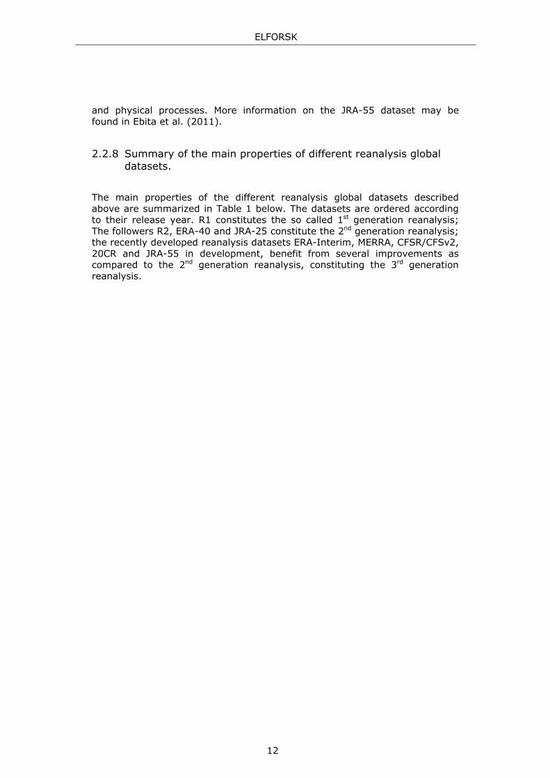
2.2.8 Summary of the main properties of different reanalysis global datasets.

The main properties of the different reanalysis global datasets described above are summarized in Table 1 below. The datasets are ordered according to their release year. R1 constitutes the so called 1st generation reanalysis; The followers R2, ERA-40 and JRA-25 constitute the 2nd generation reanalysis; the recently developed reanalysis datasets ERA-Interim, MERRA, CFSR/CFSv2, 20CR and JRA-55 in development, benefit from several improvements as compared to the 2nd generation reanalysis, constituting the 3rd generation reanalysis.

ELFORSK

13

Release year Reanalysis Institution

Horizontal resolution

lat x lon (deg)

Vertical level of interest

Temporal resolution

Data assimilation

scheme

Temporal coverage

1995 R1 NCEP/NCAR 2.5 x 2.5 0.995 sigma level 6 h 3D-Var 1948 - on

2002 R2 NCEP/NCAR 2.5 x 2.5 0.995 sigma level 6 h 3D-Var 1979 - 2010

2005 ERA-40 ECMWF 1.125 x 1.125 10 m a.g.l. 6 h 3D-var 9/1957 - 8/2002

2006 JRA-25 JMA & CRIEPI 1.25 x 1.25 10 m a.g.l. 6 h 3D-Var 1979 - 2004

2008 ERA-Interim ECMWF 0.75 x 0.75 10 m a.g.l. 6 h 4D-var 1979 - on

2009 MERRA NASA 1/2 x 2/3 50 m a.g.l. 1 h 3D-Var with incremental

update 1979 - on

2009 CFSR NCEP 0.5 x 0.5 0.995 sigma level 1 h 3D-Var 1979 - 3/2011

2010 20CRv2 NOAA-CIRES 2.0 x 2.0 0.995 sigma level 6 h Ensemble Kalmar Filter

11/1869 - 12/2010

2011 CFSv2 NCEP 0.5 x 0.5 0.995 sigma level 6 h 3D-Var 4/2011 - on

expected 2013 JRA-55 JMA --- --- --- 4D-var 1958-2012

Table 1. Main properties of different reanalysis global datasets ordered according to their release year. The background gray color with increasing darkness marks the 1st, 2nd, and 3rd generation reanalyses. The 0.995 sigma level corresponds to an altitude of about 42 m a.g.l. 1 degree latitude is equivalent to approximately 111.4 km for the latitudes of the Scandinavia, and 1 degree longitude to 55.8 km.

ELFORSK

14

2.3 Reanalysis mesoscale datasets

Since the reanalysis global datasets have typically rather coarse temporal and spatial resolutions, there is the need for datasets with finer spatial and temporal resolutions that may represent the local wind climate with higher accuracy. Mesoscale numerical models may be used to downscale reanalysis global data to a horizontal grid with finer resolution (typically 1 km x 1 km to 10 km x 10 km) and with hourly temporal resolution. The resultant long-term time series are here designated as reanalysis mesoscale datasets, but are also known as virtual time series or virtual met masts.

There is a large number of different reanalysis mesoscale datasets available in the market. Note however that none of them are publicly available. For this reason, only the two mesoscale datasets produced at Kjeller Vindteknikk have been used in the present study. These datasets are therefore briefly described below.

2.3.1 WRF FNL

WRF FNL is the name of a long-term dataset produced by Kjeller Vindteknikk using the mesoscale model WRF driven by FNL data.

The Weather Research and Forecast (WRF) model is a state-of-the-art mesoscale numerical weather prediction system, aiming at both operational forecasting and atmospheric research needs. The model version used to produce the WRF FNL dataset is version v3.2.1 described in Skamarock et al. (2008). Details on the modeling structure, numerical routines and physical packages available can be found in Klemp et al. (2000) and Michalakes et al. (2001). The development of the WRF model is supported by a strong scientific and administrative community in U.S.A. The number of users is large and is growing rapidly. The code is publicly accessible through the WRF's webpage (WRF, 2012).

The solving of the model equations requires the definition of the boundary conditions of the area of interest, as well as of the initial conditions. FiNaL operational global analysis data (FNL) produced by NCEP is used in the definition of the boundary and of the initial conditions. NCEP FNL data is available as global data with 1 degree resolution and 6 hours temporal resolution and is an analysis product from the Global Data Assimilation System (GDAS). It should be noted that NCEP FNL is an analysis product, not reanalysis, since GDAS is not kept constant in time. WRF FNL data is available for the time period 2000 to the present with a temporal resolution of 1 hour and a horizontal resolution of 4 km x 4 km.

ELFORSK

15

2.3.2 WRF ERA-Interim

WRF ERA-Interim is another long-term dataset produced at Kjeller Vindteknikk. The main difference between WRF ERA-Interim and WRF FNL is the data used in the definition of the boundary and initial conditions. ERA-Interim reanalysis data is used in this case instead of NCEP FNL analysis data. WRF ERA-Interim data is available for the period 1992 to the present with 1 hour temporal resolution and 6 km x 6 km horizontal resolution.

ELFORSK

16

3 Using reanalysis data to describe the local wind climate in terrain with low complexity

This chapter presents an analysis of the ability of reanalysis data to describe the local wind climate in terrain with low complexity. First, a discussion is presented on the temporal and spatial characteristics of reanalysis global data over the geographical region located between 54 and 72 degrees North and 4 and 32 degrees East. This region covers Norway, Sweden, Denmark, Finland and the Baltic states, and is hereafter designated by focus region. Secondly, the correlation coefficients of the relationships between reanalysis data and local wind measurements, from 42 different sites located in terrain with low complexity, are analyzed. Finally, a discussion is presented concerning the difficulties on defining the long-term data's representativeness, i.e., on defining how well long-term data from a reference site represents the long-term wind climate at the measurement site.

3.1 Analysis of the temporal and spatial characteristics of reanalysis data

Reanalysis data constitute a relevant tool in the investigation of past climate variability (Trenberth, 2010). However, the assimilating atmospheric models used in the generation of reanalysis data are prone to biases which may be corrected through the use of abundant and unbiased observations. Difficult challenges arise though when the spatial and temporal coverage of the observations are poor, and when the observations are themselves biased due to changes in the instrumentation or in the recording system. This may result in the introduction of artificial trends and low-frequency variations, i.e. inconsistencies, in the reanalysis data that are mixed with true climatic changes.

The use of reanalysis data as representative of the local long-term wind climate, and in the consequent estimate of the long-term energy production of wind farms, is a common practice. Either publicly available reanalysis global datasets, or commercial mesoscale reanalysis datasets with finer spatial and temporal resolutions, may be used. The consistency of the data is however an important issue that should be taken into account when choosing the most appropriate long-term dataset. This issue is addressed in Sections 3.1.1 and 3.1.2, below.

Long-term weather observations from climate monitoring stations may also be used in the long-term correction of wind measurements. These are however rather sparse and often affected by inhomogeneities As emphasized in Section 2.1.1, there are known limitations in the measurements from surface weather stations that may induce systematic errors in the data, requiring a

ELFORSK

17

careful cleaning of erroneous data. Data from the NCEP ADP dataset is not included in the analysis below. However, the analysis methods presented below may also be used in the analysis of these and other long-term data.

The QuickSCAT and Seawinds datasets described in Section 2.1.2 are also not investigated in this report since these datasets have terminated in 2009 and 2003, respectively, and are therefore not relevant for use in the long-term correction of ongoing measurements. Results on the analysis of QuickSCAT data may be found in e.g. Hasager et al. (2006) and Harstveit et al. (2012). Note, that the Blended Sea Winds dataset is kept current and may therefore be of interest for the long-term correction of offshore wind measurements. Nevertheless, since the geographical focus area of this study is mainly onshore, the analysis of Blended Sea Winds data is not included in this report.

3.1.1 Linear rate of change maps

In order to analyze and compare the temporal and spatial characteristics of different reanalysis datasets, the linear rate of change of the wind speed for the period 1979 to 2004 was calculated for each grid point of the reanalyses R1, JRA-25, ERA-Interim, MERRA and CFSR/CFSv2. The choice of these reanalysis datasets is based on the fact that all of them are kept current and are therefore relevant to wind resource analysis. The choice of the period 1979-2004 is justified by the fact that the JRA-25 dataset has data only until 2004, and all of them have data from 1979. Since the reanalysis mesoscale datasets WRF FNL and WRF ERA-Interim begin only on 2000 and 1992, respectively, they are not included in this analysis.

The methodology used in the calculation of the linear rate of change is illustrated in Figure 3-1 based on data for a specific grid point. The monthly average of the wind speed at 42 m a.g.l. from the R1 grid point 60.0◦ N 17.5◦

E is shown in blue for the period 1979 to 2004. The monthly averages are normalized to the mean wind speed of the entire period. The black line shows the 12-months moving average of the monthly mean wind speed. The linear function that best fits, according to the least squares principle, to the 12-months moving averaged data is shown in red.

The linear rate of change of a given wind speed series during a given time period is here defined as the slope of the linear function that best fits the 12-months moving average of the monthly mean wind speed during that period. This parameter is commonly used in climatology to measure long-term trends in different meteorological variables, such as temperature (e.g. Simmons, 2004).

ELFORSK

18

Figure 3-1. The blue line shows the monthly mean wind speed for the period 1979 to 2004 of the R1 grid point 60.0◦ N 17.5◦ E , normalized to the mean wind speed for the entire period. The 12-months moving average of the monthly mean wind speed is shown in black. The red line shows the linear function that best fits to the black curve.

Using the methodology described above, the linear rate of change of the wind speed corresponding to each grid point of the R1, JRA-25, ERA-Interim, MERRA and CFSR/CFSv2 datasets, and located within the chosen focus area, was calculated. The results are presented in the form of rate of change maps in Figure 3-2. The top panels show the rate of change maps of the surface wind speed, while the bottom panels show the rate of change maps for the wind speed at the 850 hPa pressure level retrieved from the different reanalysis datasets. The wind speed at the pressure level of 850 hPa may be considered a good approximation of the geostrophic wind, i.e., the wind driven by the balance between the Coriolis force and the pressure gradient force.

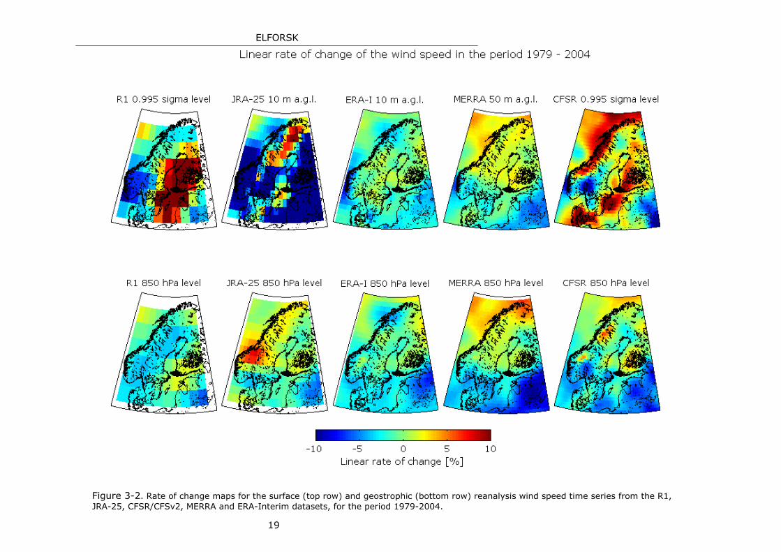
ELFORSK

19

Figure 3-2. Rate of change maps for the surface (top row) and geostrophic (bottom row) reanalysis wind speed time series from the R1, JRA-25, CFSR/CFSv2, MERRA and ERA-Interim datasets, for the period 1979-2004.

ELFORSK

20

The following conclusions may be drawn from the results presented in Figure 3-2:

The linear rate of change of the R1 and JRA-25 surface wind speed data in the period 1979-2004 shows rather large differences between the grid cells in parts of the analyzed region. These differences appear much smoother in the finer resolution datasets, particularly in ERA-Interim and MERRA.

The coarse spatial resolution of the R1 and the JRA-25 datasets (2.5x2.5 and 1.25x1.25 degrees, respectively, see Table 1) may explain the observed large differences in the linear rate of change of neighbor grid points at the surface level. Due to the large dimensions of a grid cell, the atmospheric conditions at the boundaries of a given grid cell may differ significantly at the surface level, and probably less significantly at the 850 hPa level. Consequently, larger differences in the temporal characteristics of the data for different grid points may be expected mainly at the surface level for the low resolution datasets.

The linear rate of change of the geostrophic wind (bottom panels) is more homogeneous throughout the analyzed area and varies less between the models. These results are associated with the larger spatial scale of the wind speed patterns at the 850 hPa level as compared to that at the surface level.

The rate of change maps of ERA-Interim, MERRA and CFSR/CFSv2 are rather similar to each other. At the surface level, CFSR/CFSv2 wind speed data show more extreme values as compared to ERA-Interim and MERRA. Note, however, that the answer on how the linear rate of change map should look like is not known. Therefore one can't say that a given reanalysis gives a more correct result than the other. It is though important to be aware that different reanalyses have different spatial and temporal characteristics. This has an impact in the long-term corrected wind conditions. In a case study presented by Liléo and Petrik (2011) a difference of 14 to 18 % in the estimated long-term energy at a given position was obtained, using reanalysis data from closely located grid points, associated with different linear rates of change.

Based on the conclusions presented above, we recommend the use of reanalysis wind speed data with fine spatial resolution in the long-term correction of wind measurements. Moreover, the finer resolution reanalysis datasets ERA-Interim, MERRA and CFSR/CFSv2 belong to the 3rd generation reanalysis (Table 1) which favors from advances in the assimilation techniques, as well as in the used global atmospheric model, as compared to the previous generation reanalyses. For these reasons, the reanalysis datasets R1 and JRA-25 are discarded at this point, and are therefore not included in the remaining study. An investigation study on the use of the R1 dataset in the long-term correction of wind measurements may though be found in Liléo and Petrik (2011).

ELFORSK

21

3.1.2 Decomposition into high and low-frequency components

A further analysis of the specific wind speed long-term time series intended to be used in the long-term correction of wind measurements is recommendable in order to detect possible structural changes in the data.

BFAST (Breaks For Additive Seasonal and Trend) is a technique used to detect changes in the structure of time series by decomposing the series into three different components: a periodic high-frequency component designated as seasonal component, a low-frequency component designated as trend, and a noise component (remainder). BFAST has been developed by Verbesselt et al. (2009) to detect trend and seasonal changes in the land cover using satellite image time series. Their approach may however be applied to a broad spectra of other fields including the analysis of long-term wind data. The main difference between BFAST and standard time series decomposition methods (e.g. Fourier decomposition) is that BFAST integrates the iterative decomposition of time series into trend, seasonal and noise components with methods for detecting and characterizing changes (breakpoints) within the time series. BFAST is integrated as a package in the R system for statistical computing. The package can be downloaded from the Comprehensive R Archive Network (CRAN) through the webpage CRAN (2012).

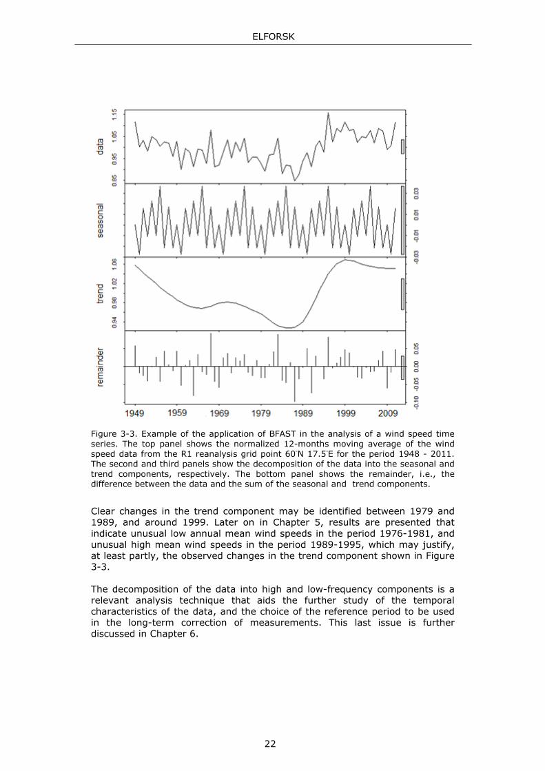
Figure 3-3 shows the decomposition of the reanalysis wind speed data (normalized 12-months moving average) from the R1 grid point 60◦N 17.5◦E into seasonal, trend and remainder components (same grid point as shown in Figure 3-1). Note that "seasonal" designates in this context the high-frequency component of the data which may have a periodicity of a couples of years, and is not necessarily related to the variation of the wind in the different seasons of the year.

The top panel shows the annual averages of the wind speed data from the 0.995 sigma level for the period 1948 - 2011. The second and third panels show the decomposition of the data into the high and low-frequency components (seasonal and trend components). The bottom panel shows the remainder, i.e., the difference between the data and the sum of the seasonal and the trend components. The solid bars on the right hand side of the panels show the same data range, to facilitate comparisons.

ELFORSK

22

Figure 3-3. Example of the application of BFAST in the analysis of a wind speed time series. The top panel shows the normalized 12-months moving average of the wind speed data from the R1 reanalysis grid point 60◦N 17.5◦E for the period 1948 - 2011. The second and third panels show the decomposition of the data into the seasonal and trend components, respectively. The bottom panel shows the remainder, i.e., the difference between the data and the sum of the seasonal and trend components.

Clear changes in the trend component may be identified between 1979 and 1989, and around 1999. Later on in Chapter 5, results are presented that indicate unusual low annual mean wind speeds in the period 1976-1981, and unusual high mean wind speeds in the period 1989-1995, which may justify, at least partly, the observed changes in the trend component shown in Figure 3-3. The decomposition of the data into high and low-frequency components is a relevant analysis technique that aids the further study of the temporal characteristics of the data, and the choice of the reference period to be used in the long-term correction of measurements. This last issue is further discussed in Chapter 6.

ELFORSK

23

3.2 Strength of the relationship to local wind measurements

Data from the reanalysis global datasets ERA-Interim, MERRA and CFSR/CFSv2 and from the reanalysis mesoscale datasets WRF FNL and WRF ERA-Interim are used in this section to analyze the strength of the relationship between reanalysis data and wind measurements. The reanalysis global datasets R1 and JRA-25 are not included in this analysis due to the reasons presented in Section 3.1.1.

3.2.1 Description of the database used A database composed by data recorded at 24 met masts placed in sites potentially suitable for wind power development, and at 18 masts belonging to meteorological stations, has been used in this study. These masts are located in Norway, Denmark and Sweden, in terrain with rather low complexity. The precise location of the masts is not presented in this report for confidentiality reasons. Data from the meteorological stations were retrieved through NCDC's Land-based Data webpage (NCDC, 2012b) for the period 2002 to 2009. Wind speed and direction data from each of the masts included in the database have been inspected manually. Erroneous data and data influenced by the formation of ice on the sensors have been removed. The measurements are from 10, 50, 80 and 100 m height, and the measurement period varies between 1 and 8 years.

3.2.2 Results The strength of the relationship between the wind speed data measured at each of the masts included in our database, and the wind speed data from the nearest located reanalysis grid point, has been measured by means of the Pearson correlation coefficient, R, calculated based on concurrent data at the highest possible temporal resolution (6 hours for ERA-Interim and CFSR/CFSv2 data and 1 hour for MERRA data), i.e., no averaging is involved. The term concurrent data is used in this report to designate data with identical time stamps.

The definition of the Pearson correlation coefficient has been adopted in this report as the measure of the strength of the relationship between two variables2. If nothing else is specified, the definition of the Pearson correlation coefficient is used whenever the term correlation coefficient is mentioned.

Surface and geostrophic wind speed data from ERA-Interim, MERRA and CFSR/CFSv2, as well as surface wind data from WRF FNL and WRF ERA-Interim have been included in this analysis. The median value of the correlation coefficients obtained for the considered sites, and for a given 2 The Pearson correlation coefficient is the most commonly used definition of the correlation coefficient. It measures the strength of the relationship between two variables, being sensitive only to a linear relationship between the variables (Wikipedia Correlation, 2012).

ELFORSK

24

reanalysis dataset, is plotted with a blue bar in Figure 3-4 below. Each bar corresponds to a reanalysis dataset. The median values are also explicitly displayed in the figure. The lower and the upper whiskers mark the minimum and the maximum values of the obtained correlation coefficients, respectively. The lower and the upper edges of the white boxes mark the first and the third quartiles, respectively. Note that the quartiles divide the samples into four equally sized parts, and that the second quartile is the same as the median (shown with the blue bars and the displayed values). Within each white box is located half of the samples. Larger boxes represent a larger dispersion of the results.

Such a box-and-whisker plot showing the minimum, the three quartiles and the maximum of the results is considered to adequately represent the distribution of the results, since the correlation coefficient has most likely a non-normal distribution (Gorsuch and Lehmann, 2010).

Figure 3-4. Box-and-whisker plot of the correlation coefficient (R) of the relationship between wind speed measurements from 42 different sites and wind speed data from the nearest located reanalysis grid point. Data from the surface level (10, 42, 50 and 100 m a.g.l.) and from the geostrophic level (850 hPa pressure level) from different reanalyses are used. The blue bars and the displayed values show the median of the results. The lower and the upper whiskers mark the minimum and the maximum values, respectively. The lower and the upper edges of the boxes mark the first and the third quartiles, respectively. The median is the same as the second quartile.

ELFORSK

25

The results presented in the figure above suggest the following conclusions:

The relationship between measured wind speed data and reanalysis geostrophic wind speed data (850 hPa level) is weaker than the relationship with reanalysis wind speed data from the surface level. This result was expected since the weather patterns in the atmosphere are shifted in time with height, and because the strength of the relationship (i.e. the correlation coefficient) is related to simultaneity (i.e. simultaneous occurrence in time).

The relationship between measured and MERRA wind speed data is, for

the majority of the analyzed cases, stronger than the relationship with the remaining reanalysis datasets. The larger correlation coefficients obtained for MERRA as compared to WRF FNL and WRF ERA-Interim suggests that a finer spatial resolution of the long-term reference data may not necessarily result in a larger correlation coefficient. The correlation coefficient calculated based on hourly values is first and foremost a measure of how well the short-term fluctuations in the reference and in the measured wind speed data agree in phase. The correlation coefficient does not measure, for example, how well the mean wind speed level of the reference data agrees with that of the measured wind. Modeled datasets with fine spatial resolution such as WRF FNL and WRF ERA-Interim may capture some properties of the local wind climate, such as the mean wind speed level, more accurately than datasets with coarser spatial resolution (e.g. MERRA). This property is of high relevance for wind resource mapping for example, but not as relevant in the long-term correction of wind measurements.

Similar analysis should be conducted for sites located in complex terrain and looking at other parameters such as the wind direction and the frequency distribution.

3.2.3 Is the correlation coefficient an appropriate measure of representativeness?

The correlation coefficient calculated based on hourly data has been used above to investigate how well different reanalysis datasets represent the local wind climate at measurement sites. However, as discussed above, a large hourly correlation coefficient is strongly associated with simultaneity, i.e., with the phase consistency of the short-term fluctuations in the reference and in the measured wind speeds. But does a good representativeness by the reference data require simultaneity? By representativeness is meant how well long-term data from a reference site represents the long-term wind variations at the measurement site. Suppose that a met mast is located at the position A and that a weather front hits A at a given instant and moves further towards position B located some kilometers away. A met mast located at B will experience similar weather as

ELFORSK

26

in A, but with some time delay, that is, not simultaneously. The correlation coefficient of the relationship between concurrent wind speed data from A and B will be low. However, the long-term data from the position A represent well the long-term variations in the wind speed at B. This example illustrates that representativeness does not require simultaneity. A case of good representativeness may result on a low correlation coefficient. Is the correlation coefficient calculated based on monthly averages of the measured and the reference wind speeds a more appropriate measure of the reference data's representativeness? The challenge when using monthly correlation coefficients is that seasonality (i.e., the seasonal variation of the wind conditions) may result being a dominant factor. Ideally, the seasonality should be removed in order to allow a better measure of the representativeness at other time scales than the seasonal. The analysis described in Section 3.2.2 was now repeated using the monthly correlation coefficient instead of the hourly correlation coefficient. Hourly correlation coefficient is here used to designate the correlation coefficient of the relationship between the measured wind speed and the concurrent reanalysis wind speed. By monthly correlation coefficient is meant the correlation coefficient of the relationship between the monthly averages of the measured wind speed and the reference (reanalysis) wind speed. Only months with a coverage of the measured data larger than 85% have been considered. The results obtained are shown in Figure 3-5 using the same format as in Figure 3-4. The comparison between the results presented in Figures 3-4 and 3-5 shows the following: The monthly correlation levels are higher than the hourly correlation levels

for all the analyzed reanalysis datasets. Particularly the reanalysis data from the 850 hPa level show a rather large relative increase when using the monthly instead of the hourly correlation coefficient. This result was expected since the monthly correlation coefficient smooth out short-term variations.

The analyzed reanalysis datasets give very similar correlation coefficients when calculated on a monthly basis, suggesting that the factors that differentiate the different reanalyses are less significant in this case as compared to on a hourly basis.

Both the hourly and the monthly correlation coefficients present limitations

on their ability to measure the reference data's representativeness. Further work should be conducted to define a more appropriate measure of representativeness.

The ability of reanalysis data to represent the wind direction distribution

as well as the frequency distribution of the wind speed at a given location has not been investigated in this study. This is however a relevant issue that should be a matter of further investigation.

ELFORSK

27

Figure 3-5. Box-and-whisker plot of the correlation coefficient (R) of the relationship between the monthly averages of the measured wind speed from 42 different sites and of the wind speed data from the nearest located reanalysis grid point. Only the months with a data coverage of the site measurements larger than 85% have been considered. The lower and the upper whiskers mark the minimum and the maximum values, respectively. The lower and the upper edges of the white boxes mark the first and the third quartiles, respectively. The median is the same as the second quartile, and is shown with the blue bars and with the displayed values.

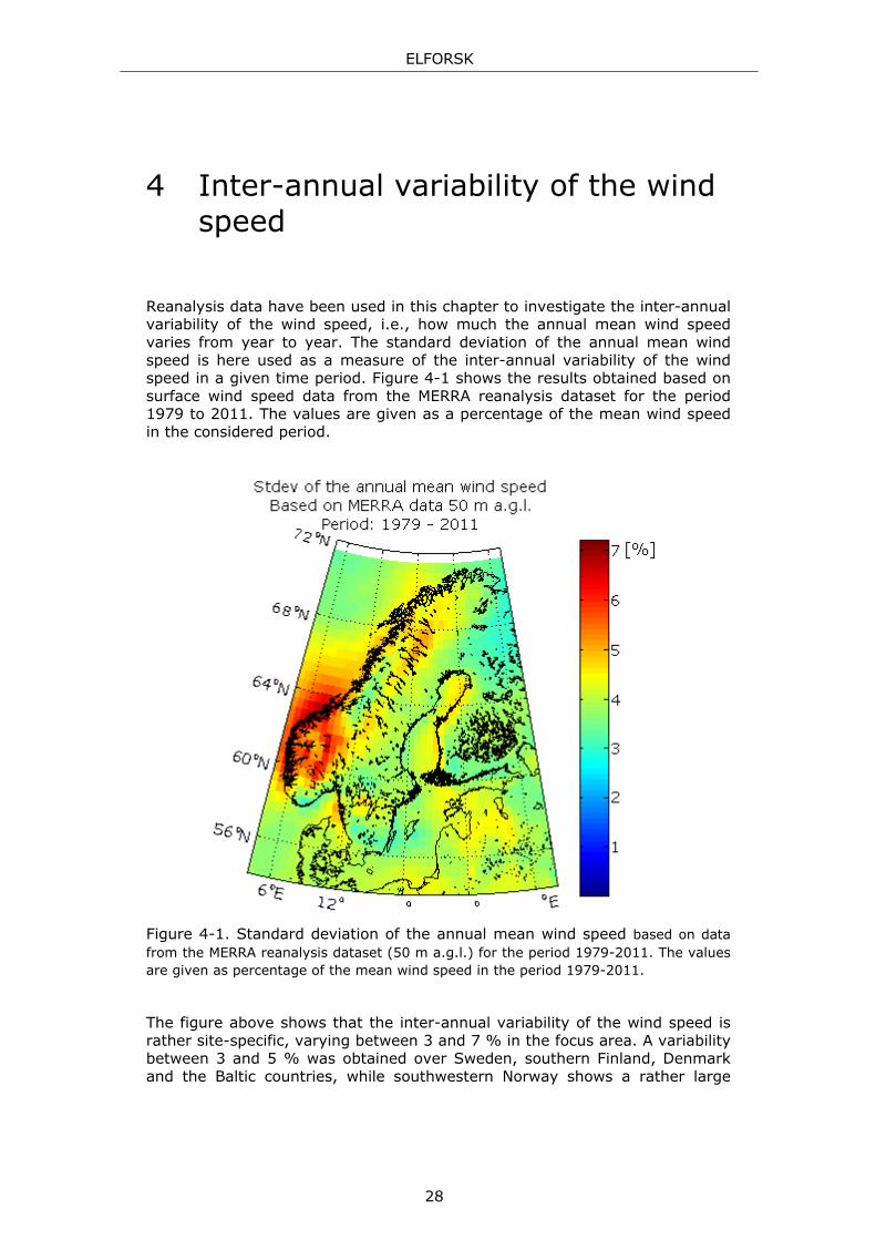
ELFORSK

28

4 Inter-annual variability of the wind speed

Reanalysis data have been used in this chapter to investigate the inter-annual variability of the wind speed, i.e., how much the annual mean wind speed varies from year to year. The standard deviation of the annual mean wind speed is here used as a measure of the inter-annual variability of the wind speed in a given time period. Figure 4-1 shows the results obtained based on surface wind speed data from the MERRA reanalysis dataset for the period 1979 to 2011. The values are given as a percentage of the mean wind speed in the considered period.

Figure 4-1. Standard deviation of the annual mean wind speed based on data from the MERRA reanalysis dataset (50 m a.g.l.) for the period 1979-2011. The values are given as percentage of the mean wind speed in the period 1979-2011.

The figure above shows that the inter-annual variability of the wind speed is rather site-specific, varying between 3 and 7 % in the focus area. A variability between 3 and 5 % was obtained over Sweden, southern Finland, Denmark and the Baltic countries, while southwestern Norway shows a rather large

ELFORSK

29

variability (up to 7 %), and northern Norway and Finland rather low (down to about 2.5 %).

A similar analysis was conducted based on MERRA and WRF ERA-Interim data for the 20-year period 1992-2011. The results are presented in Figure 4-2. Note that the WRF ERA-Interim dataset available at the moment covers only part of the focus area.

The inter-annual variability of the MERRA mean wind speed in the periods 1979-2011 and 1992-2011 has very similar amplitudes. It is not possible to do such a comparison based on WRF ERA-Interim data, since this dataset covers only the period 1992-2011. However, it is interesting to compare the MERRA and the WRF ERA-Interim wind variability for the period 1992-2011 (Figure 4-2). A slightly larger wind variability is observed in the WRF ERA-Interim data as compared to MERRA data, particularly over Sweden. This result may be coupled to the finer spatial resolution of the WRF ERA-Interim data allowing for a more accurate description of the local wind variability.

In a publication by EWEA (2009), the inter-annual variability of the wind speed was investigated based on long-term datasets of about 30 years in duration. The authors concluded that although the variability of the wind speed is site specific, it tends to be similar across Europe, and can reasonably be assumed to be about 6 %. It is however our opinion that the inter-annual variability of the wind speed should be estimated specifically for the site in consideration, instead of assuming a general value.

The knowledge on the inter-annual variability of the wind speed is important for the following reasons:

The inter-annual variability of the wind speed is an important source of uncertainty in the estimate of the energy production of a wind farm. A variation of the annual mean wind speed of 3 to 7 % corresponds to a variation of the annual energy production of a wind farm of about 8 to 18 % (assuming a factor of 2.5 between change in energy and change in wind speed; this factor does however vary from case to case). It is therefore important to be aware that the annual energy production of a wind farm may deviate from the expected value by about 8 to 18 % (depending on the location of the wind farm), just due to the intrinsic variability of the wind. The awareness of this fact is important for the investors, as well as for the electric utilities that handle the energy production.

Locations with an expected large wind variability may require longer measurement periods in order to allow a better description of the local wind climate, not only in terms of the wind speed but also in terms of wind direction, stability, wind shear and turbulence.

As a further study it would be interesting to analyze the inter-annual variability of the wind direction, stability, wind shear and turbulence. No publications have been found on these issues.

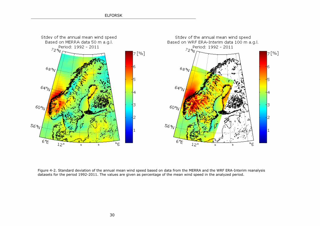
ELFORSK

30

Figure 4-2. Standard deviation of the annual mean wind speed based on data from the MERRA and the WRF ERA-Interim reanalysis datasets for the period 1992-2011. The values are given as percentage of the mean wind speed in the analyzed period.

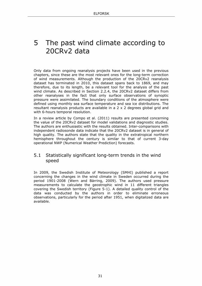
ELFORSK

31

5 The past wind climate according to 20CRv2 data

Only data from ongoing reanalysis projects have been used in the previous chapters, since these are the most relevant ones for the long-term correction of wind measurements. Although the production of the 20CRv2 reanalysis dataset has terminated in 2010, this dataset spans back to 1869, and may therefore, due to its length, be a relevant tool for the analysis of the past wind climate. As described in Section 2.2.4, the 20CRv2 dataset differs from other reanalyses in the fact that only surface observations of synoptic pressure were assimilated. The boundary conditions of the atmosphere were defined using monthly sea surface temperature and sea ice distributions. The resultant reanalysis products are available in a 2 x 2 degrees global grid and with 6-hours temporal resolution.

In a review article by Compo et al. (2011) results are presented concerning the value of the 20CRv2 dataset for model validations and diagnostic studies. The authors are enthusiastic with the results obtained. Inter-comparisons with independent radiosonde data indicate that the 20CRv2 dataset is in general of high quality. The authors state that the quality in the extratropical northern hemisphere throughout the century is similar to that of current 3-day operational NWP (Numerical Weather Prediction) forecasts.

5.1 Statistically significant long-term trends in the wind speed

In 2009, the Swedish Institute of Meteorology (SMHI) published a report concerning the changes in the wind climate in Sweden occurred during the period 1901-2008 (Wern and Bärring, 2009). The authors used pressure measurements to calculate the geostrophic wind in 11 different triangles covering the Swedish territory (Figure 5-1). A detailed quality control of the data was conducted by the authors in order to eliminate erroneous observations, particularly for the period after 1951, when digitalized data are available.

ELFORSK

32

Figure 5-1. Definition of the triangles used in the calculation of the geostrophic wind performed by Wern and Bärring (2009). Pressure measurements from the stations marked with blue dots were used. The red dots mark the locations of alternative stations used when data from the main stations are missing (from Wern and Bärring, 2009).

Based on the geostrophic wind speed calculated for each of the triangles shown in the figure above, Wern and Bärring (2009) estimated the linear rate of change of the geostrophic wind speed in the period 1951 to 2008. The results obtained by the authors are presented in Table 2 below. Aiming to compare these results with the equivalent values based on the 20CRv2 dataset, wind speed data from the 0.995 sigma level of the 20CRv2 dataset have been used to estimate the linear rate of change of the wind speed in the period 1951 to 2008, for each of the triangles shown in the figure above. The results obtained are also included in Table 2 below.

ELFORSK

33

Linear rate of change of the wind speed during the period 1951-2008 (%)

Triangle Results obtained by Wern

and Bärring (2009) based on geostrophic wind speed.

Results based on surface wind speed data from the

20CRv2 dataset

1 -3 1.7

2 4 -0.8

3 -1 1.0

4 -2 0.6

5 -2 2.5

6 -3 0.4

7 -10 0.3

8 -10 -0.9

9 -6 1.1

10 -8 -0.9

11 -2 -1.2 Mean value -4 0.3

Table 2. Comparison between the linear rate of change of the geostrophic wind speed obtained by Wern and Bärring (2009) for the period 1951-2008, and the linear rate of change of the 20CRv2 wind speed at the 0.995 sigma level during the same period.

There is a general disagreement of the results both in sign and magnitude. The results obtained using the 20CRv2 dataset do not confirm the decreasing trend concluded by Wern and Bärring (2009) for the wind speed in Sweden during the period 1951-2008. Although a great work has been conducted by Wern and Bärring (2009) to eliminate erroneous data from the used database, surface pressure observations may be affected by systematic errors that may still prevail. On the other hand, the 20CRv2 assimilation system includes an improved methodology for bias correction of pressure observations that may be more efficient on removing systematic errors in the assimilated data. Furthermore, as noted by Wern and Bärring (2009), results from trend analysis should not be used to draw conclusions on the long-term variation of the wind climate if the estimated trends are not statistically significant. A statistically significant trend means that the probability of that trend will occur given no linear long-term variation in the data series, is lower than 5% (Wikipedia, Statistical significance, 2012). Wern and Bärring analyzed the significance of the estimated trends and concluded that only for 4 of the 11 triangles the obtained trends are statistically significant.

The left panel in Figure 5-2 shows the linear rate of change map of the 20CRv2 wind speed for the period 1951 to 2008. This map is the basis of the

ELFORSK

34

results presented in Table 2 above. The statistical significance (p-level) of the rate of change values shown in this map has been estimated and is presented in the right panel of Figure 5-2. A value is significant if the corresponding p-level is lower than 0.05.

The results show that the significance of the estimated linear rate of change values is rather weak for most of the grid points located in the Swedish territory (p larger than 0.05). It may therefore be concluded that neither the results presented by Wern and Bärring (2009) nor the results based on 20CRv2 data indicate a statistically significant long-term trend in the wind speed over Sweden during the period 1951-2008.

However, the slightly increasing long-term trend observed in the 20CRv2 wind speed data over the coastal and inland regions of central and northern Norway, appears to be statistically significant, since the corresponding linear rate of change values are associated to rather low p-values (the smaller the p-level, the more significant the trend).

ELFORSK

35

Figure 5-2. Left panel: rate of change map of the wind speed based on 20CRv2 reanalysis data for the period 1951-2008. Right panel: Statistical significance (p-level) of the estimated linear rate of change values shown in the left panel. A value is significant if the corresponding p-level is lower than 0.05.

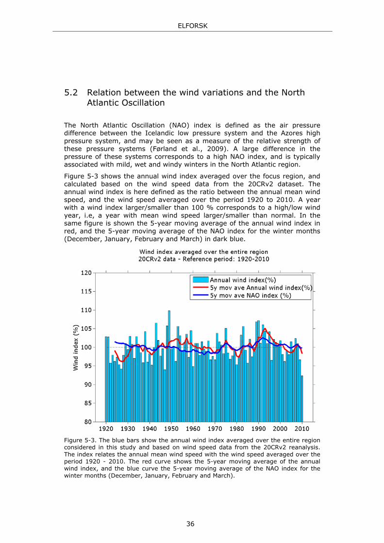
ELFORSK

36

5.2 Relation between the wind variations and the North Atlantic Oscillation

The North Atlantic Oscillation (NAO) index is defined as the air pressure difference between the Icelandic low pressure system and the Azores high pressure system, and may be seen as a measure of the relative strength of these pressure systems (Førland et al., 2009). A large difference in the pressure of these systems corresponds to a high NAO index, and is typically associated with mild, wet and windy winters in the North Atlantic region.

Figure 5-3 shows the annual wind index averaged over the focus region, and calculated based on the wind speed data from the 20CRv2 dataset. The annual wind index is here defined as the ratio between the annual mean wind speed, and the wind speed averaged over the period 1920 to 2010. A year with a wind index larger/smaller than 100 % corresponds to a high/low wind year, i.e, a year with mean wind speed larger/smaller than normal. In the same figure is shown the 5-year moving average of the annual wind index in red, and the 5-year moving average of the NAO index for the winter months (December, January, February and March) in dark blue.

Figure 5-3. The blue bars show the annual wind index averaged over the entire region considered in this study and based on wind speed data from the 20CRv2 reanalysis. The index relates the annual mean wind speed with the wind speed averaged over the period 1920 - 2010. The red curve shows the 5-year moving average of the annual wind index, and the blue curve the 5-year moving average of the NAO index for the winter months (December, January, February and March).

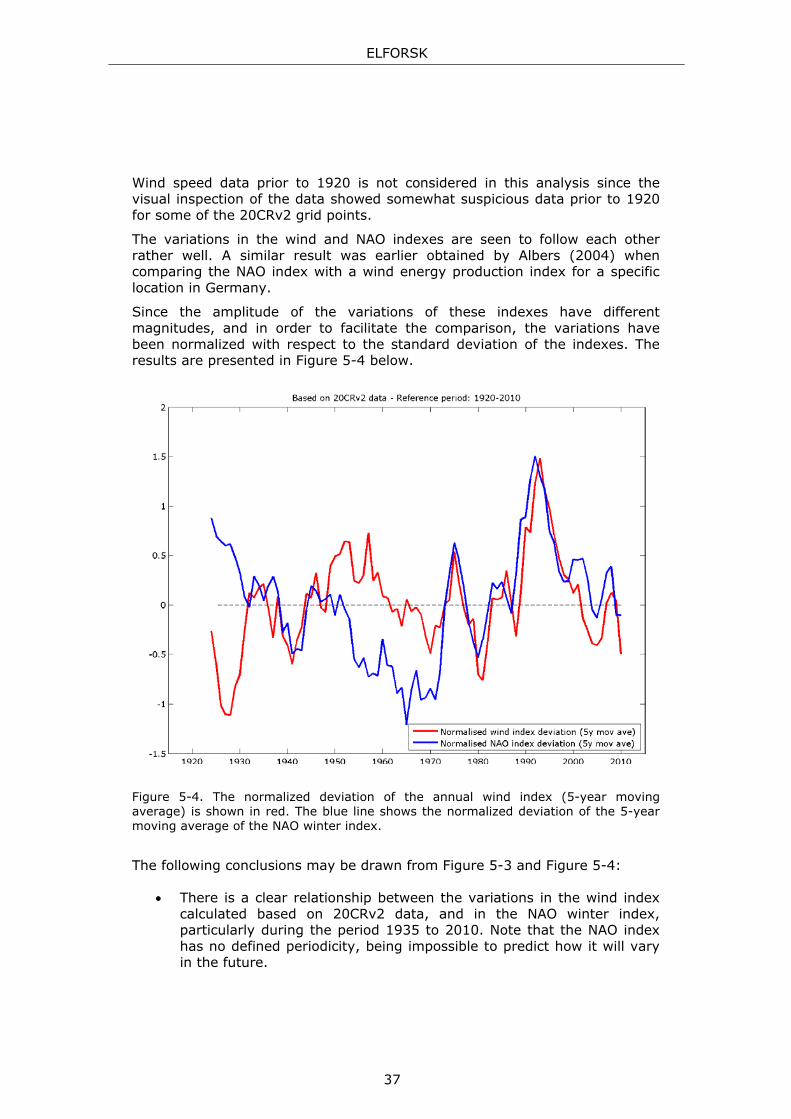
ELFORSK

37

Wind speed data prior to 1920 is not considered in this analysis since the visual inspection of the data showed somewhat suspicious data prior to 1920 for some of the 20CRv2 grid points.

The variations in the wind and NAO indexes are seen to follow each other rather well. A similar result was earlier obtained by Albers (2004) when comparing the NAO index with a wind energy production index for a specific location in Germany.

Since the amplitude of the variations of these indexes have different magnitudes, and in order to facilitate the comparison, the variations have been normalized with respect to the standard deviation of the indexes. The results are presented in Figure 5-4 below.

Figure 5-4. The normalized deviation of the annual wind index (5-year moving average) is shown in red. The blue line shows the normalized deviation of the 5-year moving average of the NAO winter index.

The following conclusions may be drawn from Figure 5-3 and Figure 5-4:

There is a clear relationship between the variations in the wind index calculated based on 20CRv2 data, and in the NAO winter index, particularly during the period 1935 to 2010. Note that the NAO index has no defined periodicity, being impossible to predict how it will vary in the future.

ELFORSK

38

The period 1989 to 1995 was characterized by unusual high annual mean wind speeds associated with a large positive peak in the NAO index.

The decrease in the mean wind speed seen between 1990 and 2005 represents a return to the longer-term mean, after the unusual large maximum in 1990. This result is in accordance with the conclusions by Thomas et al (2009) obtained based on different windiness indexes for northern Europe.

The period 1976 - 1981 had unusual low annual mean wind speeds associated with a dip in the NAO index. The period 1922 - 1928 was also a low wind speed period, however not consistent with a dip in the NAO index.

In the next chapter, the influence of the choice of the reference period in the estimate of the long-term corrected wind speed is investigated, benefiting from the results presented in this chapter.

ELFORSK

39

6 Choice of the reference period

The main purpose of long-term correction of wind measurements is to estimate the future long-term wind conditions at a given site potentially suitable to wind power development. However, since it is not possible to predict how the wind will vary in the next decades, the past is normally used as a predictor of the future wind climate. In other words, it is assumed that the wind conditions will vary in the next decades in a similar way as they did in the past. But how certain is this assumption? It is important to evaluate the uncertainty associated with this assumption and to account for it in the total uncertainty of long-term corrected wind. Another important issue is the choice of the past period that is assumed to be representative of the future wind variations. This period is hereafter designated as the reference period. The uncertainty in the estimated long-term corrected wind should also account for the uncertainty inferred by the choice of the reference period. In this chapter, wind speed data from the 20CRv2 reanalysis surface level for the period 1951 to 2010 is used to estimate the uncertainty associated with the assumption that the future wind climate will vary in a similar way as in the past. Furthermore, this data is also used to analyze how the uncertainty in the long-term corrected wind depends on the choice of the reference period.

6.1 Accuracy in the assumption of the past being a predictor of the future wind conditions

As concluded in Section 5.2, the period 1989 to 1995 was characterized by unusual high annual mean wind speeds, followed by years with lower mean wind speeds. Looking at Figure 6-1 below, one may guess that the mean wind speed in the period 1996-2010 is fairly lower than the mean wind speed in the precedent period with the same length (15 years). The comparison between the mean wind speeds in these two periods is of interest, since it gives an estimate of the error in using the past to predict the future in a worst-case scenario. How large is the prediction error in this case? In order to answer to this question, the mean wind speeds of the reference period (1981-1995) and of the future period (1996-2010) were calculated based on wind speed data from each grid point of the 20CRv2 dataset located in the focus region. The percentage difference between the reference and the future mean wind speeds is here defined as the prediction error. The prediction error was calculated based on wind speed data from each grid point. The results are shown in Figure 6-2 below.

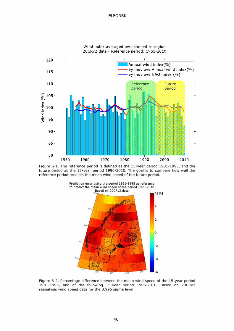
ELFORSK

40

Figure 6-1. The reference period is defined as the 15-year period 1981-1995, and the future period as the 15-year period 1996-2010. The goal is to compare how well the reference period predicts the mean wind speed of the future period.

Figure 6-2. Percentage difference between the mean wind speed of the 15-year period 1981-1995, and of the following 15-year period 1996-2010. Based on 20CRv2 reanalysis wind speed data for the 0.995 sigma level

Referenceperiod

Future period

ELFORSK

41

Figure 6-2 shows that using the 15-year period 1981-1995 to predict the mean wind speed of the following 15-year period results in an overestimation of the wind speed of about 2 to 6 %. The 15-year period 1981-1995 is therefore not a good predictor of the following 15-year period. The main reason is the unusual high mean wind speeds observed in 1989-1995, and the subsequent decrease to normal values. Is the prediction error lower if the reference period is chosen from within the interval 1951-1988 preceding the high wind period 1989-1995? In order to answer to this question the reference period was set as a 15-year moving window defined within the period 1951 - 1988, as illustrated in the figure below.

Figure 6-3. Illustration of the method used to estimate the error in the prediction of the mean wind speed for the future period, if the reference period is set as a 15-year moving window defined within 1951 - 1988.

There are 25 different 15-year broad windows in the period 1951 - 1988. The mean wind speed of each of these windows (reference periods) was calculated and then compared to the mean wind speed of the future period. The prediction error for each case is, as previously, defined as the percentage difference between the mean wind speeds of the reference period and of the future period. The absolute prediction error averaged over all the 25 different cases is presented in Figure 6-4 below.

Referenceperiod 15 y

Future period 15 y

ELFORSK

42

Figure 6-4. Average of the absolute prediction error obtained using different periods of 15 consecutive years chosen among 1951 - 1988 to predict the mean wind speed of the period 1996-2010. The results are based on 20CRv2 wind speed data at the 0.995 sigma level.

The error in the prediction of the mean wind speed for the period 1996 - 2010 is in this case about 1 to 2 % for the majority of the focus area. This is much lower than the prediction error (2 to 6 %) obtained using the precedent 15-year period (1981 - 1995) as reference period (Figure 6-2). This analysis illustrates that not always the near past is the best predictor of the near future. For the case analyzed above, choosing a reference period from the far past resulted in a lower prediction error. The accuracy in the assumption of using the past as a predictor of the future wind climate is further discussed in Section 6.3.

6.2 Random and consecutive sampling Random sampling of the years composing the reference period was also tested against consecutive sampling. The results presented in Figure 6-4 correspond to consecutive sampling, i.e., the reference period is composed by 15 consecutive years. How would the result differ if the years composing the reference period are chosen randomly instead for consecutively from within the period 1951 - 1988? Figure 6-5 shows the difference between the absolute mean prediction error obtained using random sampling and that

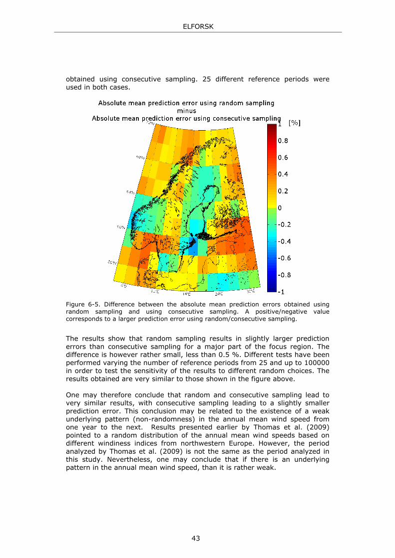
ELFORSK

43

obtained using consecutive sampling. 25 different reference periods were used in both cases.

Figure 6-5. Difference between the absolute mean prediction errors obtained using random sampling and using consecutive sampling. A positive/negative value corresponds to a larger prediction error using random/consecutive sampling.

The results show that random sampling results in slightly larger prediction errors than consecutive sampling for a major part of the focus region. The difference is however rather small, less than 0.5 %. Different tests have been performed varying the number of reference periods from 25 and up to 100000 in order to test the sensitivity of the results to different random choices. The results obtained are very similar to those shown in the figure above. One may therefore conclude that random and consecutive sampling lead to very similar results, with consecutive sampling leading to a slightly smaller prediction error. This conclusion may be related to the existence of a weak underlying pattern (non-randomness) in the annual mean wind speed from one year to the next. Results presented earlier by Thomas et al. (2009) pointed to a random distribution of the annual mean wind speeds based on different windiness indices from northwestern Europe. However, the period analyzed by Thomas et al. (2009) is not the same as the period analyzed in this study. Nevertheless, one may conclude that if there is an underlying pattern in the annual mean wind speed, than it is rather weak.

ELFORSK

44

6.3 Dependence of the prediction error on the reference period length

The following analysis concerns the evaluation of the error in the predicted future mean wind speed as a function of the length of the chosen reference period. The method used in this analysis is illustrated in Figure 6-6 and is described below.

Figure 6-6. Illustration of the method used to estimate the influence of the reference period length in the error of the estimated mean wind speed for the future period.

The length of the future period is set to 20 years (typical lifetime of a

wind farm) and the period moves within the interval 1952 to 2010.

The reference period is always chosen as adjacent (precedent) to the reference period and is composed by consecutive years.

The length of the reference period is allowed to vary between 1 and 30 years. Note that the reference period length could vary up to 40 years, but since the number of possible periods longer than 30 years is rather low, a maximum period length of 30 years is defined.

The percentage difference between the mean wind speeds of the reference and future periods is calculated for each case, and is designated as the prediction error.

Reference period Varying length: 1 to 30 years Moving period

Future period Const. length: 20y Moving period

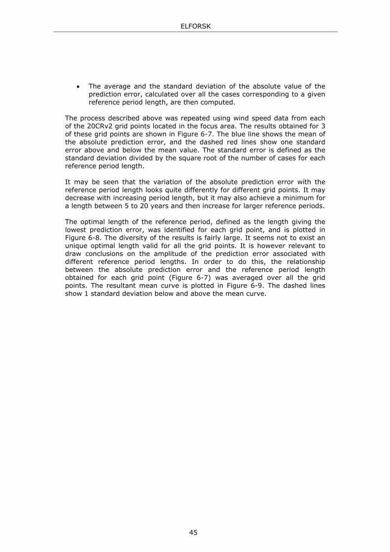
ELFORSK

45

The average and the standard deviation of the absolute value of the

prediction error, calculated over all the cases corresponding to a given reference period length, are then computed.

The process described above was repeated using wind speed data from each of the 20CRv2 grid points located in the focus area. The results obtained for 3 of these grid points are shown in Figure 6-7. The blue line shows the mean of the absolute prediction error, and the dashed red lines show one standard error above and below the mean value. The standard error is defined as the standard deviation divided by the square root of the number of cases for each reference period length. It may be seen that the variation of the absolute prediction error with the reference period length looks quite differently for different grid points. It may decrease with increasing period length, but it may also achieve a minimum for a length between 5 to 20 years and then increase for larger reference periods. The optimal length of the reference period, defined as the length giving the lowest prediction error, was identified for each grid point, and is plotted in Figure 6-8. The diversity of the results is fairly large. It seems not to exist an unique optimal length valid for all the grid points. It is however relevant to draw conclusions on the amplitude of the prediction error associated with different reference period lengths. In order to do this, the relationship between the absolute prediction error and the reference period length obtained for each grid point (Figure 6-7) was averaged over all the grid points. The resultant mean curve is plotted in Figure 6-9. The dashed lines show 1 standard deviation below and above the mean curve.

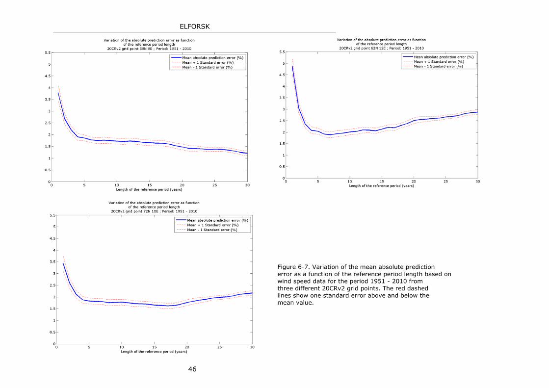
ELFORSK

46

Figure 6-7. Variation of the mean absolute prediction error as a function of the reference period length based on wind speed data for the period 1951 - 2010 from three different 20CRv2 grid points. The red dashed lines show one standard error above and below the mean value.

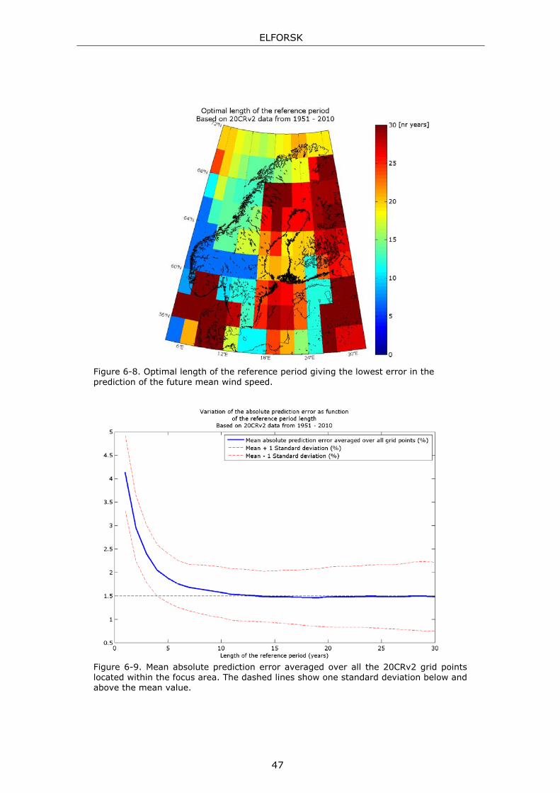
ELFORSK

47

Figure 6-8. Optimal length of the reference period giving the lowest error in the prediction of the future mean wind speed.

Figure 6-9. Mean absolute prediction error averaged over all the 20CRv2 grid points located within the focus area. The dashed lines show one standard deviation below and above the mean value.

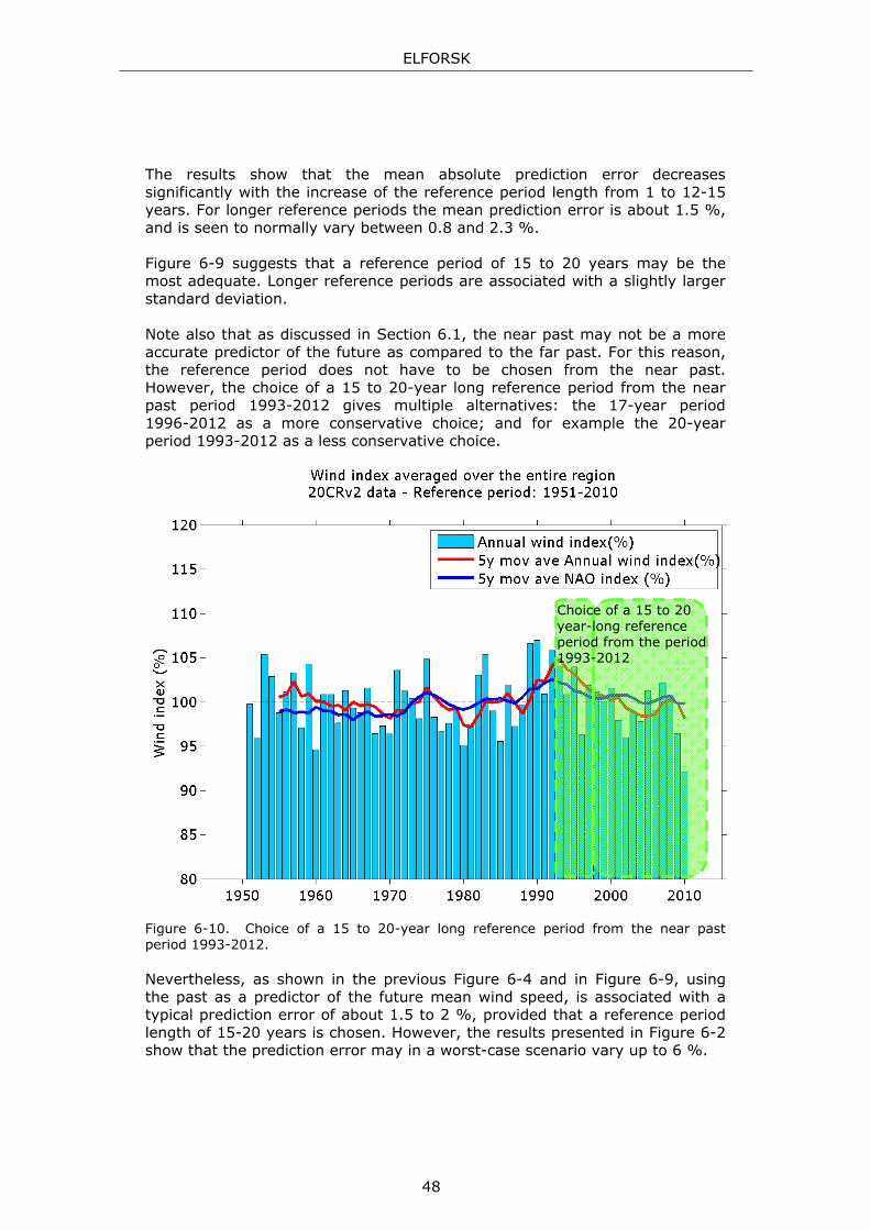
ELFORSK

48

The results show that the mean absolute prediction error decreases significantly with the increase of the reference period length from 1 to 12-15 years. For longer reference periods the mean prediction error is about 1.5 %, and is seen to normally vary between 0.8 and 2.3 %. Figure 6-9 suggests that a reference period of 15 to 20 years may be the most adequate. Longer reference periods are associated with a slightly larger standard deviation. Note also that as discussed in Section 6.1, the near past may not be a more accurate predictor of the future as compared to the far past. For this reason, the reference period does not have to be chosen from the near past. However, the choice of a 15 to 20-year long reference period from the near past period 1993-2012 gives multiple alternatives: the 17-year period 1996-2012 as a more conservative choice; and for example the 20-year period 1993-2012 as a less conservative choice.

Figure 6-10. Choice of a 15 to 20-year long reference period from the near past period 1993-2012. Nevertheless, as shown in the previous Figure 6-4 and in Figure 6-9, using the past as a predictor of the future mean wind speed, is associated with a typical prediction error of about 1.5 to 2 %, provided that a reference period length of 15-20 years is chosen. However, the results presented in Figure 6-2 show that the prediction error may in a worst-case scenario vary up to 6 %.

Choice of a 15 to 20 year-long reference period from the period 1993-2012

ELFORSK

49

7 Long-term correction methods

Different methodologies have been developed to long-term correct wind measurements. A common property of all of them is their main purpose: to describe the long-term wind climate at a specific site, based on short-term measurements performed at the site (hereafter called short-term site measurements), and long-term data available from a representative location (hereafter called long-term reference data). The main differences between the different methodologies consist on how the comparison between site and reference data is performed, and on how the sought long-term wind climate at the site is calculated.

Table 3 presents commonly used long-term correction methods (LTC methods) grouped according to the methodology used in the comparison of the site and reference data.

Category Method's name Developer

Regression LTC methods

Least squares regression Regression MCP EMD, WindPRO

Least Squares method GL-GH, WindFarmer

Principal component regression PCA method GL-GH, WindFarmer

Quantile regression U&N method KVT, internal use

Non-regression LTC methods

Linear scaling methods Weibull Scale MCP EMD, WindPRO

Wind Index MCP EMD, WindPRO

T&N method KVT, internal use

KH method KVT, internal use

Probabilistic LTC methods Matrix Method MCP EMD, WindPRO

Table 3. Categorization of commonly used long-term correction methods.

The different LTC methods may be grouped into two main categories: regression LTC methods and non-regression LTC methods. Section 7.1 presents a description of the main properties of the different LTC methods included in Table 3. An analysis of the performance of the different methods is presented in Section 7.2.

ELFORSK

50

7.1 Description of different LTC methods

7.1.1 Regression LTC methods

Regression analysis is a statistical technique commonly used to find the relationship between two variables. In the context of long-term correction of wind measurements, regression analysis is used to find the relationship between the wind climate at the reference position and the wind climate at the measurement site. Regression analysis may be performed based on different techniques. Some of these are for example the least squares, the principal component and the quantile regression techniques. Four different LTC methods developed based on one of these regression techniques have been analyzed. These are the Regression MCP method, the Least Squares method, the PCA method and the U&N method.

Least squares regression methods

Regression MCP

Regression MCP is the name of a regression LTC method developed by EMD International A/S and implemented in the WindPRO software package. The Regression MCP method applies a regression model to the relationship between the short-term site wind speed and the concurrent reference wind speed, as well as to the relationship between the short-term wind veer and the concurrent reference wind speed. The parameter wind veer is defined as the change in wind direction between the site and the reference positions. A special characteristic of the Regression MCP method is the inclusion of a model for the distribution of the wind speed and wind veer residuals.

Let us suppose that y represents the site wind speed or direction measurements and x the reference concurrent wind data. After performing a regression analysis to x and y, a regression function is obtained describing the relationship between these parameters. This function is here denominated as f(x). y' = f(x) is the fitted value, whereas the difference between the fitted and the original values (y'-y) is designated as the residual, . In another words, is the bias (error) of the fitting process for the specific pair (x,y).

For each pair (xi, yi) of the concurrent time series, a residual j corresponding to the pair (xj, yj) is randomly chosen, and then added to yi. The regression model initially applied to (xi, yi) is then reapplied to the set of values (xi, yi+j), and a new fitted function is obtained. Residual resampling consists on repeating this process a statistically significant number of times. This technique allows the use of the information regarding the scatter of the regression analysis in the estimation of statistical properties of the dataset.

WindPRO allows the user to choose if the function (x) is modeled as a 1st or 2nd order polynomial. Furthermore, the user may also choose between different orders of polynomial functions to be applied in the regression analysis of the wind speed and wind veer. The default alternatives presented

ELFORSK

51

in WindPRO are a linear (1st order polynomial) regression model for the wind speed, and a constant (0th order polynomial) model for the wind veer. A 1st order Gaussian model is recommended to be used as the residual model of the wind speed, and no residual resampling is recommended to be applied to the wind direction. These default alternatives have been used when applying the Regression MCP model in the performance analysis presented in Section 3.2.

The user is also given the opportunity to choose whether the transfer function that will be applied to the long-term reference data should be found for different moving sectors of a given width and 1 degree step (e.g. 360 overlapping sectors being each of them 30 deg broad), or for a user-defined number of non-overlapping sectors with uniform width (e.g. 12 non-overlapping sectors 30 deg broad). The default alternative is the first one. This alternative has been chosen in the comparison study presented in Section 3.2.

The long-term time series at the site position is then finally estimated by applying the transfer functions to the long-term reference data.

More information on this method may be found in Thøgersen et al. (2010b) and Thøgersen and Sørensen (2007).

Linear Squares method

The software package WindFarmer developed by GL Garrad Hassan includes a LTC method named the Least Squares method. This method is based on the standard linear regression technique and consists on the calculation of the linear function that best fits the relationship between the short-term wind speed at the site position (y) and the concurrent wind speed at the reference position (x). The linear fit is calculated by minimizing the sum of the squared distances between each measured value, yi, and the corresponding fitted value yi'. The regression analysis is performed sectorwise using an user-inferred number of direction bins.

WindFarmer allows the user to choose whether to force the fit to pass through the origin or not. The user is also given the opportunity to adjust the settings for cut off wind speeds used in the regression analysis. In this way, data at low wind speeds may be excluded from the regression analysis.

The linear function resultant from the regression analysis is then applied to the long-term reference wind speed in order to calculate the long-term site wind speed. This may be done sectorwise (default option) or the user may choose to apply a fixed correction factor for all the direction bins. The long-term wind direction at the site is assumed by default to be the same as the long-term wind direction at the reference position. However, the user may choose to apply sectorwise shifts or a constant shift to the reference wind direction.

A detailed description of this method may be found in the WindFarmer's theory manual (Garrad Hassan & Partners, 2011).

ELFORSK

52

Principal component regression methods

PCA method

PCA stands for Principal Component Analysis and is a LTC method available through the software WindFarmer. This method is based on the principal component regression technique and seeks to find the direction (y*) along which a given variable presents the greatest variance. Let's suppose that the variable B is linearly correlated to the variable A, and that we plot B along the y-axis and A along the x-axis. The direction y* along which B has the greatest variance is called the principal component, and x* which is orthogonal to y* is the second principal component. The idea is that if the variables A and B are plotted in the coordinate system (x*,y*), then B does not longer depend on A, i.e., these variables become linearly uncorrelated. Figure 7-1 illustrates this technique.

Figure 7-1. Illustration of the coordinate systems (x,y) and (x*,y*), where y* is the principal component, and x* the second principal component of the variable B.

The PCA method consists on the calculation of the linear function that minimizes the distance d (shown in Figure 7-1) between the site wind speed y and the fitted wind speed y', measured along the direction y*. This is performed sectorwise using an user-inferred number of direction bins.

WindFarmer allows the user to choose whether to force the fit to pass through the origin or not. As for the Linear Squares method, the resultant regression function may be applied sectorwise (default option) or a fixed correction factor may be chosen for all the direction bins. The long-term wind direction at the site is assumed by default to be the same as the long-term wind direction at the reference position. However, the user may choose to apply sectorwise shifts or a constant shift to the reference wind direction.

ELFORSK

53

More information on this method may be found in the WindFarmer's theory manual (Garrad Hassan & Partners, 2011).

Quantile regression methods

U&N method

The U&N method is a LTC method recently developed by Ove Undheim and Finn Nyhammer at Kjeller Vindteknikk. This method is used solely in-house at Kjeller Vindteknikk and is based on the quantile regression technique. This technique consists in applying regression analysis to the relationship between the quantile3 values of two datasets, instead of the dataset values themselves. By describing the relationship between the quantile values, the temporal dimension of the datasets is ignored. That is, the datasets are not ordered according to a time stamp, but according to the quantile order. This methodology ensures that the statistical properties (mean value, standard deviation and others) of the site wind speed and direction distributions are correctly described in the estimated site long-term wind speed and wind direction time series. The present version of the U&N method focuses on the description of the wind direction and wind speed. A relevant further development of this method would be to include the description of the atmospheric stability.

A detailed description of this method is attached in Appendix.

7.1.2 Non-regression LTC methods

The second main category presented in Table 3 refers to non-regression LTC methods. This category includes LTC methods that do not include a description of the relationship between site wind measurements and concurrent reference wind data based on regression analysis. Two subcategories are presented: Linear scaling methods and Probabilistic LTC methods. The methods included in each of these subcategories are described below.

3 Quantiles are points taken at regular intervals from the cumulatitive distribution function of a variable. For example, the 1st 4-quantile of a variable is the value such that the probability of the variable being less than this value is at most 1/4. For the 3rd 4-quantile, the corresponding probability is 3/4. One can then say that the kth q-quantile of a variable is the value such that the probability of the variable being less than this value is at most k/q (Wikipedia Quantile, 2012).

ELFORSK

54

Linear scaling methods

Weibull Scale MCP

The Weibull Scale MCP method here described is implemented in WindPRO and consists in a simple empirical method that assumes a linear scaling between the measured site and the concurrent reference Weibull scale parameter (k), Weibull form parameter (A), occurrence frequency and mean wind speed. More specifically, the ratio between the measured site and the concurrent reference Weibull parameter A, Weibull parameter k, occurrence frequency and mean wind speed are calculated for each of 12 equally broad direction bins. These ratios are here designated as sectorwise correction values. The sectorwise mean values of the parameters A and k, as well as the sectorwise occurrence frequency and mean wind speed of the long-term reference data are then multiplied by the corresponding sectorwise correction values. In this way, a sectorwise description of the long-term Weibull distribution for the site wind speed is obtained. Note that since this method only transforms the parameters A, k, occurrence frequency and the mean wind speed, no long-term site time series is calculated. A strong sectorwise correlation between the site measurements and the reference data is needed in order to ensure a good accuracy of this method. Furthermore, the method will fail to predict wind climates described by non-Weibull distributions.

This method is further described in Thøgersen et al. (2010b) and Thøgersen and Sørensen (2007).

Wind Index MCP

A LTC method named Wind Index MCP is available in WindPRO. This method assumes that the ratio between the short-term4 and the long-term average power outputs at the site is equal to the corresponding ratio at the reference position. That is, if the average short-term power output at the reference position was X% of the long-term power output at that position, then the short-term average power output at the measurement site should also be x% of the corresponding long-term average power output. In this way, the expected long-term average power output at the site may be calculated from the measured short-term site power output and the known short and long-term average power outputs at the reference location. A special property of this method is that the averaging is performed on a monthly basis.

Since this method works with the power output instead of the wind speed, a power curve must be chosen to convert wind speed to power. The user is given the opportunity to choose between a real power curve specific to a given turbine model, and a generic power curve where the power is assumed to increase with the square of increasing wind speeds until the rated power is reached. For larger wind speeds the power output is kept constant and equal

4 By site short-term data is meant the measured data; reference short-term data refers to the reference data with the same time stamps (concurrent) as the measured data.

ELFORSK

55

to the rated power. Furthermore, the reference power output should be representative of the site power output. Consequently, the reference mean wind speed is scaled such that it equals the site mean wind speed at the height of interest. This value is user-inferred and is recommended to be defined as the expected site mean wind speed at hub height.

More information on this method may be found in Thøgersen et al. (2010b) and Thøgersen and Sørensen (2007).

T&N method

The T&N method was developed by Tallhaug and Nygaard and published in 1993 (Tallhaug and Nygaard, 1993). This method is a development of the method originally presented by Nygaard (1992) and is one of the LTC methods used at Kjeller Vindteknikk. For each direction bin of the reference short-term data, the mean and the standard deviation of the site and of the reference short-term wind speeds are calculated, as well as the correlation coefficient of their relationship. The long-term mean wind speed at the site for each direction bin of the long-term reference data may be estimated using the following formula

_ _ ∙ _

_∙ _ _ Eq. 1

where s stands for site, r for reference, st and lt for short and long-term respectively, for mean wind speed, for standard deviation and R for correlation coefficient. The superscript i designates the direction bin at the reference position.

Since Eq. 1 gives the site long-term mean wind speed conditioned to the reference wind direction bin, it is now necessary to calculate the long-term wind speed conditioned to the site wind direction, that is, to calculate the site long-term mean wind speed for a given site wind direction bin j. The following equation is used

_ ∑ _ ∙ ∙ , Eq. 2

where pji is the probability of the direction bin j occurring at the site simultaneous with the direction bin i occurring at the reference, and is calculated based on the concurrent data. pi is the probability of the direction bin i occurring at the reference during the short-time period, and pj represents the probability of the direction bin j occurring at the site during the short-term period.

Note that this method includes the correlation coefficient of the relationship between site and reference data (calculated based on concurrent data at the

ELFORSK

56

finest possible time resolution, typically that of the reference data) explicitly in the estimation of the site long-term wind data (Eq. 1), but it does not use the regression function of this relationship. Since this method does not involve regression analysis (just correlation analysis) it is not classified as a Regression LTC method. The strength of the relationship between measured site data and concurrent reference data is however important for the accuracy of the method.

KH method

The KH method was presented by Knut Harstveit (2004) and is a LTC method used at Kjeller Vindteknikk. This method sorts the non-zero reference and the site concurrent wind speed data according to the respective wind direction data into 12 equally broad direction bins (boxes), and the zero wind speed values into a 13th box. In this way, the site data is sorted into 13 different boxed and the reference into another 13 different boxes. The average wind speed for each box is then calculated and weighted according to the occurrence frequency of that specific box. Next, the ratios between the reference and site weighted averages are calculated for each box. These ratios are hereafter designed as correction factors. Although the correction factors are calculated based on short-term data, they are assumed to be valid also in the long-term period. Based on this assumption, the weighted average of the reference long-term data for each box is then multiplied by the corresponding correction factor. In this way, the site long-term sectorwise mean wind speed is obtained. The KH method is less susceptible to the strength of the relationship between concurrent site and reference data, than the T&N method, since the correlation coefficient is not explicitly included in the calculations. Moreover, the KH method reduces the effects of the data dispersion when the correlation is poor since it uses the mean wind speed for each box. More information on this method may be found in Harstveit (2004).

Matrix MCP method

The Matrix MCP method here described is available through the software package WindPRO. This method calculates the wind speed-up and the wind veer as the differences between the site and the reference concurrent wind speed and wind direction, respectively, and then sorts the results according to the reference wind speed and wind direction. In this way, two matrixes are created, one for the wind speed-up and the other for the wind veer, where each entry corresponds to a user-inferred reference wind speed bin (default value is 1 m/s) and reference wind direction bin (default value is 30 degrees). These matrixes are the core elements of the Matrix MCP method. Figure 7-2 illustrates an example of a wind speed-up matrix.

Since some entries of the matrixes may be empty, a polynomial fit is applied to some statistical properties of the wind speed-up and wind veer in order to fill the gaps in the matrixes. The statistical properties chosen to be fitted are the mean value, the standard deviation and the correlation coefficient of the

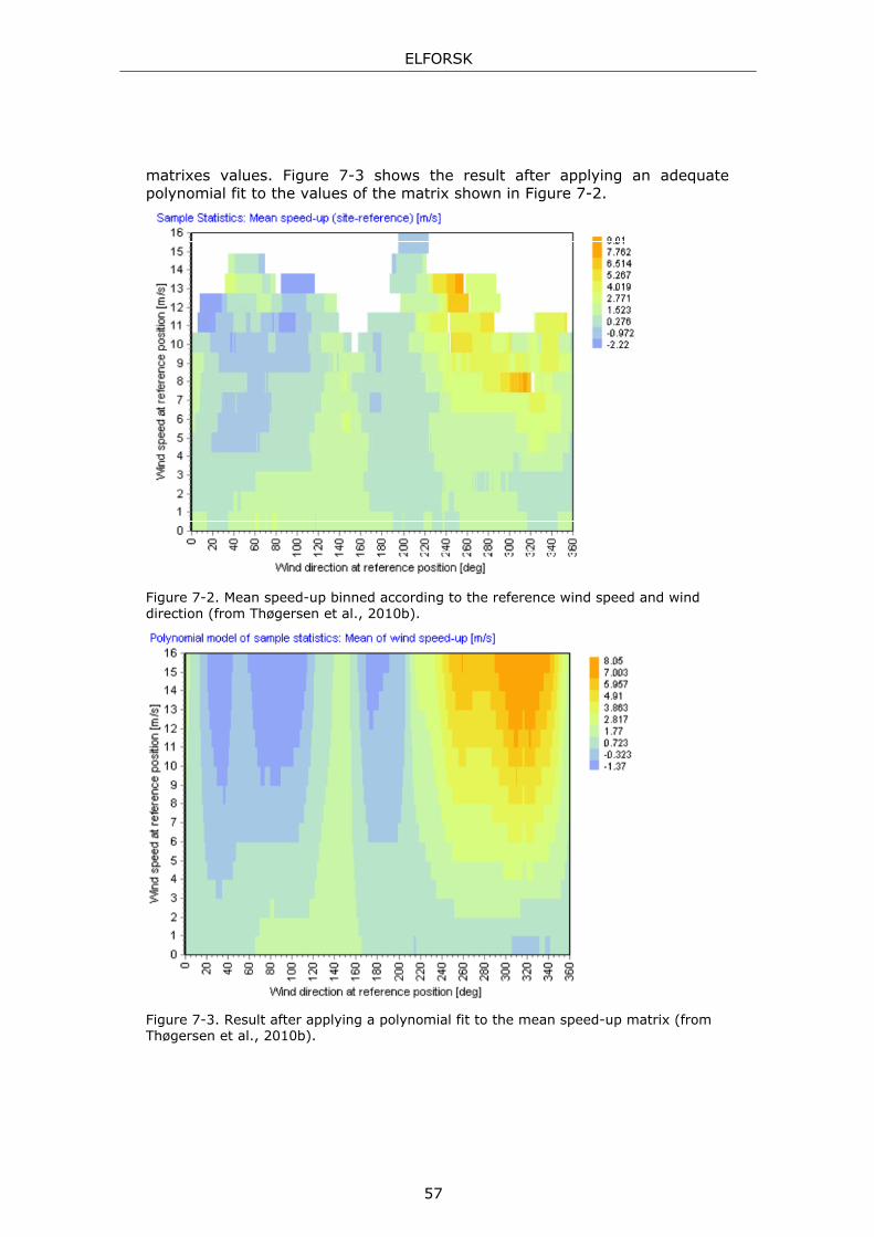
ELFORSK

57

matrixes values. Figure 7-3 shows the result after applying an adequate polynomial fit to the values of the matrix shown in Figure 7-2.

Figure 7-2. Mean speed-up binned according to the reference wind speed and wind direction (from Thøgersen et al., 2010b).

Figure 7-3. Result after applying a polynomial fit to the mean speed-up matrix (from Thøgersen et al., 2010b).

ELFORSK

58

The next step consists on transforming the reference long-term wind speed and direction series into the corresponding site long-term time series, which are the main target of this process. In order to do this, the Matrix MCP model presents two alternatives: either to model the wind speed-up and the wind veer as a function of the reference wind speed and direction by using the measured samples in each matrix entry and the corresponding probability distribution, or to use the fitted polynomial functions together with a bivariate Gaussian distribution5 of the wind speed-up and wind veer occurrence frequency. The option set as default in WindPRO is the first one if the number of samples in the matrix entry of interest is at least 5. Otherwise, the second alternative is chosen.

The long-term time series of the reference wind speed and wind direction are then transformed to the corresponding time series at the site position by applying either bootstrapping (if the first abovementioned alternative is chosen) or Monte-Carlo simulation (if the second alternative is chosen instead) to randomly create samples of wind speed and direction based on the long-term reference wind distribution. These randomly created samples are then converted to the corresponding site values by applying the wind speed-up and wind veer matrixes. The use of these probabilistic techniques in the calculation of the site long-term data justifies the categorization of the Matrix MCP method as a probabilistic LTC method.

A detailed description of the Matrix MCP method may be found in Thøgersen et al. (2010b) and Thøgersen and Sørensen (2007).

7.2 Uncertainty associated with the different LTC methods

A set composed by 16 different masts have been selected from the database presented in Section 3.2.1, to analyze the performance of the different LTC methods. The selected masts fulfill the following criteria:

More than 24 months of data.

Data coverage larger than 85 %.

Hourly correlation coefficient (R) between site and reference data larger than 80 %.

The main goal of this analysis is to estimate the error in the long-term corrected mean wind speed by testing the results from the different LTC methods against a known result, i.e., performing a self-prediction test. The procedure used is illustrated in Figure 7-4 and is described below.

5 A bivariate Gaussian distribution is a generalization of the one-dimensional Gaussian distribution to higher dimensions. The plot of the bivariate Gaussian distribution is in this case a 3-dimensional plot where the x and y axes show the wind speed-up and the wind veer, and the z axis shows the frequency according to the Gaussian function of the simultaneous occurrence of a given wind speed-up and wind veer bin.

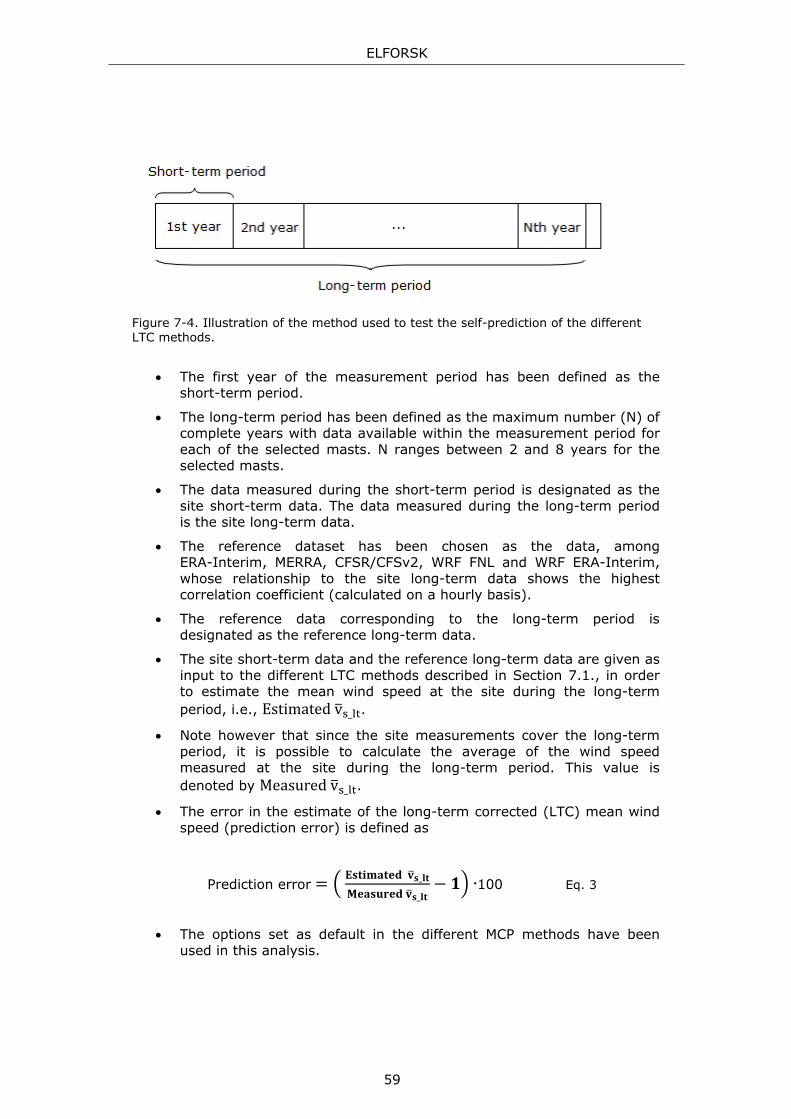
ELFORSK

59

Figure 7-4. Illustration of the method used to test the self-prediction of the different LTC methods.

The first year of the measurement period has been defined as the

short-term period.

The long-term period has been defined as the maximum number (N) of complete years with data available within the measurement period for each of the selected masts. N ranges between 2 and 8 years for the selected masts.

The data measured during the short-term period is designated as the site short-term data. The data measured during the long-term period is the site long-term data.

The reference dataset has been chosen as the data, among ERA-Interim, MERRA, CFSR/CFSv2, WRF FNL and WRF ERA-Interim, whose relationship to the site long-term data shows the highest correlation coefficient (calculated on a hourly basis).

The reference data corresponding to the long-term period is designated as the reference long-term data.

The site short-term data and the reference long-term data are given as input to the different LTC methods described in Section 7.1., in order to estimate the mean wind speed at the site during the long-term period, i.e., Estimatedv _ .

Note however that since the site measurements cover the long-term period, it is possible to calculate the average of the wind speed measured at the site during the long-term period. This value is denoted by Measuredv _ .

The error in the estimate of the long-term corrected (LTC) mean wind speed (prediction error) is defined as

Prediction error _

_∙100 Eq. 3

The options set as default in the different MCP methods have been

used in this analysis.

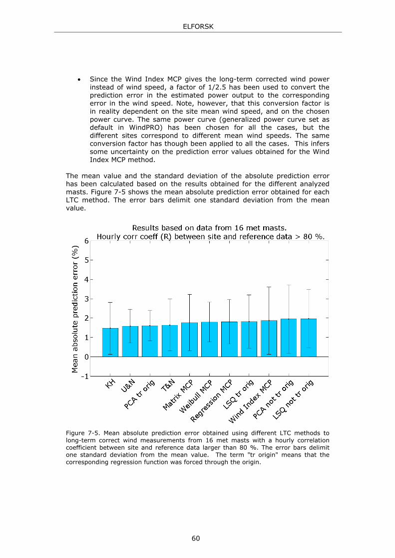
ELFORSK

60

Since the Wind Index MCP gives the long-term corrected wind power instead of wind speed, a factor of 1/2.5 has been used to convert the prediction error in the estimated power output to the corresponding error in the wind speed. Note, however, that this conversion factor is in reality dependent on the site mean wind speed, and on the chosen power curve. The same power curve (generalized power curve set as default in WindPRO) has been chosen for all the cases, but the different sites correspond to different mean wind speeds. The same conversion factor has though been applied to all the cases. This infers some uncertainty on the prediction error values obtained for the Wind Index MCP method.

The mean value and the standard deviation of the absolute prediction error has been calculated based on the results obtained for the different analyzed masts. Figure 7-5 shows the mean absolute prediction error obtained for each LTC method. The error bars delimit one standard deviation from the mean value.

Figure 7-5. Mean absolute prediction error obtained using different LTC methods to long-term correct wind measurements from 16 met masts with a hourly correlation coefficient between site and reference data larger than 80 %. The error bars delimit one standard deviation from the mean value. The term "tr origin" means that the corresponding regression function was forced through the origin.

ELFORSK

61

The results presented in Figure 7-5 show that the absolute error obtained in the estimate of the long-term mean wind speed is in average about 1.5 to 2 % for the tested LTC methods. The maximum standard deviation observed is about 1.8 %, meaning that in about 68 % of the analyzed masts the prediction error deviates at maximum about 1.8 % from its mean value. It is important to point out that the ranking shown in Figure 7-5 is not statistically significant, meaning by this that it is susceptible to the set of site and reference data used in the analysis. Particularly, the correlation coefficient between the site and reference data used in the analysis is expected to affect the performance of the different methods. Figure 7-6 shows a change in the average performance of the different LTC methods when 2 other met masts with lower correlation coefficient (75 to 80 %) were added to the database. Furthermore, the mean absolute prediction error shows a slight increase for most of the methods.

Figure 7-6. Mean absolute prediction error calculated based on 18 met masts with a correlation coefficient between site and reference data larger than 75 %. The error bars delimit one standard deviation from the mean value. The term "tr origin" means that the corresponding regression function was forced through the origin.

The performance of a similar analysis based on cases characterized by a low correlation coefficient would be of interest in order to evaluate the performance of the different models for such cases.

ELFORSK

62

7.3 Dependence of the prediction error on the measurement period length

The database used in the previous section will now be used to investigate on the influence of the measurement period length on the error of the estimated long-term corrected wind speed. The methodology used is the following:

The long-term period has been defined as the maximum number of complete years with available data. This is the same definition as the one used in the previous section and illustrated in Figure 7-4.

The short-term period is here varied from 2 months to the maximum possible number of months within the long-term period, by steps of 2 months.

The site short-term data and the reference long-term data (the meaning of these terms, and the choice of the reference data, are the same as described in the previous section) are given as input to the following LTC methods: T&N, KH and U&N method.

The reason for the choice of these methods is because they allow the automatic performance of this exercise. The consideration of the other methods described in Section 7.1 would also have been relevant, but would have been very time-consuming, since the change of the short-term period has to be done manually.

The prediction error obtained based on each of the considered short-term periods is then calculated using Eq. 3. The results are shown in Figure 7-7.

ELFORSK

63

Figure 7-7. Mean absolute prediction error as a function of the measurement period length. The results are based on data from 16 different masts with a hourly correlation coefficient between site and reference data larger than 80 %. The LTC methods used are the KH, T&N and U&N methods.

The mean absolute prediction error is seen to strongly decrease with the increase of the measurement period (concurrent period) length from 2 to 12 months. A further decrease of the mean prediction error from about 1.8 to 0.8 % is seen when the measurement period length is increased from 1 to 3 years. Note also the increase in the prediction error when slightly more than 1 and than 2 years of measurements are used. This might be related to a bias introduced by the unequal representation of each month. The use of complete years of measurements is recommended.

The accuracy of the U&N method appears to become lower than the accuracy of the KH and T&N methods for longer measurement periods. The reason for the lower performance of the U&N method for longer measurement periods should be further investigated. Applying quantile regression also to the stability conditions of the site and reference positions may contribute to the improvement of the method's performance (see Appendix).

The dashed lines in Figures 7-8 to 7-10 show one standard deviation below and above the mean value of the absolute prediction error, for the KH, T&N and U&N methods, respectively. The standard deviation of the mean absolute prediction error decreases with increasing length of the measurement period when using the KH and T&N methods, while it slightly increases for the U&N method, reflecting its lower accuracy for longer measurement periods.

ELFORSK

64

Figure 7-8. Mean absolute prediction error as a function of the measurement period length when using the KH method. The dashed lines show one standard deviation below and above the mean value.

Figure 7-9. Mean absolute prediction error as a function of the measurement period length when using the T&N method. The dashed lines show one standard deviation below and above the mean value.

ELFORSK

65

Figure 7-10. Mean absolute prediction error as a function of the measurement period length when using the U&N method. The dashed lines show 1 standard deviation below and above the mean value.

The main conclusions drawn from the results presented in this chapter are the following:

The error in the estimate of the long-term corrected wind speed is

about 1.5 to 2 % independently on the LTC method applied, provided that the hourly correlation coefficient between site measurements and reference data is greater than 75-80%, and that 1 year of site measurements with high data coverage is used. The standard deviation from the mean value may vary up to about 2 %.

Increasing the length of the measurement period from 1 to 2 years is

seen to reduce the prediction error to slightly over 1 %. This result was obtained using the KH and the T&N methods.

The use of complete years of measurements is recommended.

The evaluation of the performance of the different LTC methods for

cases with low correlation coefficient would be of interest.

ELFORSK

66

ELFORSK

67

8 Conclusions

The main conclusions obtained in the present work are summarized below.

Chapter 2 Description of different long-term reference datasets

A rather large number of datasets covering a long time period back in time are available either publicly or for purchase. These datasets may be surface and satellite observations, as well as reanalysis global datasets and finer resolution reanalysis mesoscale datasets. The main properties of some of these datasets are described in Chapter 2.

Chapter 3 Using reanalysis data to describe the local wind climate in terrain with low complexity

The coarse spatial resolution of the R1 (2.5 x 2.5 degrees) and of the JRA-25 (1.25 x 1.25 degrees) reanalysis datasets make these data less suitable to the use in the long-term correction of wind measurements. A rather large difference is observed in the linear rate of change pattern of these datasets as compared to that of the finer resolution datasets ERA-Interim, MERRA and CFSR/CFSv2, which show rather similar patterns between each other.

The use of decomposition techniques (e.g. BFAST) is recommended in order to further analyze the temporal characteristics of a specific wind speed time series, prior to its use in the long-term correction of wind measurements.

In terrain with low complexity, the hourly correlation coefficient of the relationship between MERRA surface wind speed data and measured wind speed is, for the majority of the analyzed cases, larger (median R = 0.85) than using other reanalysis global datasets (median R = 0.80), and slightly larger than using the reanalysis mesoscale datasets WRF ERA-Interim and WRF FNL (median R = 0.83). These results suggest that MERRA, as well as WRF ERA-Interim and WRF FNL, are, among the selected datasets, the most suitable to the use in the long-term correction of wind measurements performed in terrain with low complexity. The results also suggest that the increase of the spatial resolution of a long-term dataset to finer than about 0.5 x 0.5 degrees in latitude and longitude (~55 km x 30 km) does not necessarily result in the increase of the hourly correlation coefficient of its relationship to site wind measurements.

The monthly correlation coefficients obtained for different reanalysis surface datasets are very similar (0.94-0.95), suggesting that the influence of the factors differentiating these datasets is smoothed out when analyzing the data on a monthly basis.

ELFORSK

68

Neither the hourly nor the monthly correlation coefficients are an ideal measure of the reference data's representativeness. By representativeness it is meant how well the reference data describe the long-term wind variations at the measurement site. The hourly correlation coefficient is strongly influenced by simultaneity (i.e., phase consistency) which is not a necessary requirement of representativeness. On the other hand, the monthly correlation coefficient is influenced by seasonality which masks the representativeness at shorter time scales. This issue should be further investigated.

Chapter 4 Inter-annual variability of the wind speed

The inter-annual variability of the wind speed is rather site specific and should therefore be evaluated specifically for the site in consideration. Values ranging between about 3 and 7 % are found in the analyzed region (Norway, Denmark, Sweden, Finland and the Baltic countries), based on reanalysis data.

Larger spatial variations are seen in the inter-annual variability of the wind speed when calculated based on WRF ERA-Interim data (finer resolution) as compared to using MERRA data.

The performance of a study on the ability of WRF ERA-Interim and of MERRA data to describe the inter-annual variability of the wind speed would be of interest.

Chapter 5 The past wind climate according to 20CRv2 data

The 20CRv2 reanalysis dataset spans about 140 years, from the end of 1869 to the end of 2010. This dataset differs from other reanalyses in the fact that only surface observations of synoptic pressure were assimilated. Previous published studies (e.g. Compo et al., 2011) have shown that the 20CRv2 data appear to be of fairly good quality.

In an earlier study by Wern and Bärring (2009), an average negative long-term trend (-4%) was found in the wind speed in Sweden for the period 1951 to 2008. The authors emphasized though that this trend was not statistically significant. The results presented here based on 20CRv2 data confirm that there is no statistically significant trend in the wind speed during that period in Sweden (+0.3 % and not statistically significant).

20CRv2 wind speed data show a positive long-term trend (~2-3 %) over central and northern Norway in the period 1951-2008 which appears to be statistically significant. A similar analysis based on another long-term reference dataset would be of interest.

There is a clear relationship between the variations in the annual wind index calculated based on 20CRv2 data, and in the NAO winter index, particularly during the period 1935 to 2010. Note that the NAO index has no defined periodicity (Førland et al., 2009), being impossible to predict how it will vary in the future.

ELFORSK

69

The period 1989 to 1995 was characterized by unusual high annual

mean wind speeds associated with a large positive peak in the NAO index.

The decrease in the mean wind speed seen between 1990 and 2005 represents a return to the longer-term mean, after the unusual large maximum in 1990. This result is in accordance with the conclusions by Thomas et al (2009) obtained based on different windiness indexes for northern Europe.

Chapter 6 Choice of the reference period

The near past may not be a more accurate predictor of the future as compared to the far past. As an example, the mean wind speed during the 15-year period 1981-1995 was, in the analyzed region, about 2-6 % larger than the mean wind speed during the following 15-year period 1996-2010. The unusual high wind period observed in 1989-1995 explains this large prediction error.

The comparison of the mean wind speed in other reference periods from the far past (prior to 1981-1995), with the mean wind speed in the period 1996-2010, shows on average a prediction error of about 1-2 %.

Random and consecutive sampling of the years forming the reference period lead to very similar results, with consecutive sampling resulting in a slightly smaller prediction error. This conclusion suggests the existence of a weak underlying pattern (non-randomness) in the annual mean wind speed from one year to the next.

The results show the non-existence of an optimal reference period length valid for all the grid points, i.e., valid over the entire analyzed region. By optimal reference period length it is meant the length of the reference period giving the lowest prediction error. This length is seen to vary between 7 and 30 years based on 20CRv2 data for the analyzed region.

However, the results show that the mean prediction error decreases significantly with the increase of the reference period length from 1 to about 12-15 years, remaining in average rather constant (1.5 %) for longer reference periods. The standard deviation shows however a slight increase for lengths larger than 20 years. Based on these results, the choice of a reference period length of about 15 to 20 years appears reasonable.

The choice of a 15 to 20-year long reference period from the near past period 1993-2012 gives multiple alternatives: the 17-year period 1996-2012 as a more conservative choice; and for example the 20-year period 1993-2012 as a less conservative choice.

The assumption of the past being a predictor of the future mean wind speed is associated with a typical prediction error of about 1.5 to 2 %, provided that a reference period length of 15-20 years is chosen.

ELFORSK

70

However, the prediction error may in a worst-case scenario vary up to 6 %. These values are based on the analysis of the wind speed variations, occurred in the past 60-year period 1951 to 2010, according to 20CRv2 data. Possible future climate changes that may lead to smaller or larger wind variations as compared to those occurred in the past, are not considered.

Chapter 7 Long-term correction methods

A description of the main properties of the most commonly used LTC methods is given in Section 7.1.

The error in the estimate of the long-term corrected wind speed is seen to be in average about 1.5 to 2 % independently on the LTC method applied, provided that a long-term reanalysis dataset with fine spatial resolution is chosen as reference data; the hourly correlation coefficient of the relationship between reference and site data is rather large (>75-80%), and 1 year of site wind measurements with a data coverage (after quality control filtrering) larger than 85 % is used. The average error is seen to normally vary up to about 4 % (mean value plus standard deviation of the mean value).

Increasing the length of the measurement period from 1 to 2 years may reduce the average prediction error from 1.5-2 % to a level close to 1 %, when using the KH and the T&N methods.

The prediction error is seen to increase when slightly more than 1 and than 2 years of measurements are used. This might be related to a bias introduced by the unequal representation of each month. The use of complete years of measurements is recommended.

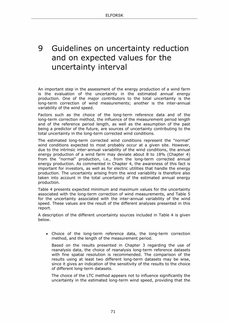
ELFORSK

71

9 Guidelines on uncertainty reduction and on expected values for the uncertainty interval

An important step in the assessment of the energy production of a wind farm is the evaluation of the uncertainty in the estimated annual energy production. One of the major contributors to the total uncertainty is the long-term correction of wind measurements; another is the inter-annual variability of the wind speed.

Factors such as the choice of the long-term reference data and of the long-term correction method, the influence of the measurement period length and of the reference period length, as well as the assumption of the past being a predictor of the future, are sources of uncertainty contributing to the total uncertainty in the long-term corrected wind conditions.

The estimated long-term corrected wind conditions represent the "normal" wind conditions expected to most probably occur at a given site. However, due to the intrinsic inter-annual variability of the wind conditions, the annual energy production of a wind farm may deviate about 8 to 18% (Chapter 4) from the "normal" production, i.e., from the long-term corrected annual energy production. As commented in Chapter 4, the awareness of this fact is important for investors, as well as for electric utilities that handle the energy production. The uncertainty arising from the wind variability is therefore also taken into account in the total uncertainty of the estimated annual energy production.

Table 4 presents expected minimum and maximum values for the uncertainty associated with the long-term correction of wind measurements, and Table 5 for the uncertainty associated with the inter-annual variability of the wind speed. These values are the result of the different analyses presented in this report.

A description of the different uncertainty sources included in Table 4 is given below.

Choice of the long-term reference data, the long-term correction method, and the length of the measurement period.

Based on the results presented in Chapter 3 regarding the use of reanalysis data, the choice of reanalysis long-term reference datasets with fine spatial resolution is recommended. The comparison of the results using at least two different long-term datasets may be wise, since it gives an indication of the sensitivity of the results to the choice of different long-term datasets.

The choice of the LTC method appears not to influence significantly the uncertainty in the estimated long-term wind speed, providing that the

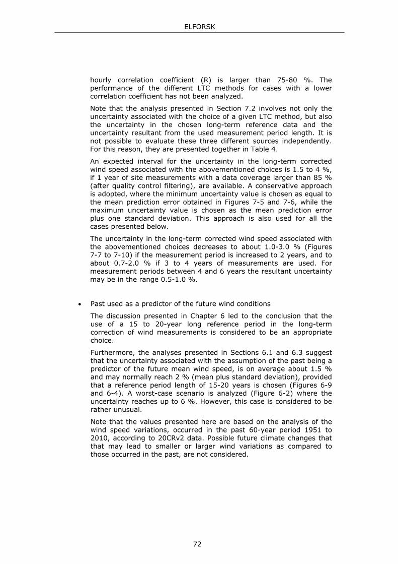
ELFORSK

72

hourly correlation coefficient (R) is larger than 75-80 %. The performance of the different LTC methods for cases with a lower correlation coefficient has not been analyzed.

Note that the analysis presented in Section 7.2 involves not only the uncertainty associated with the choice of a given LTC method, but also the uncertainty in the chosen long-term reference data and the uncertainty resultant from the used measurement period length. It is not possible to evaluate these three different sources independently. For this reason, they are presented together in Table 4.

An expected interval for the uncertainty in the long-term corrected wind speed associated with the abovementioned choices is 1.5 to 4 %, if 1 year of site measurements with a data coverage larger than 85 % (after quality control filtering), are available. A conservative approach is adopted, where the minimum uncertainty value is chosen as equal to the mean prediction error obtained in Figures 7-5 and 7-6, while the maximum uncertainty value is chosen as the mean prediction error plus one standard deviation. This approach is also used for all the cases presented below.

The uncertainty in the long-term corrected wind speed associated with the abovementioned choices decreases to about 1.0-3.0 % (Figures 7-7 to 7-10) if the measurement period is increased to 2 years, and to about 0.7-2.0 % if 3 to 4 years of measurements are used. For measurement periods between 4 and 6 years the resultant uncertainty may be in the range 0.5-1.0 %.

Past used as a predictor of the future wind conditions

The discussion presented in Chapter 6 led to the conclusion that the use of a 15 to 20-year long reference period in the long-term correction of wind measurements is considered to be an appropriate choice.

Furthermore, the analyses presented in Sections 6.1 and 6.3 suggest that the uncertainty associated with the assumption of the past being a predictor of the future mean wind speed, is on average about 1.5 % and may normally reach 2 % (mean plus standard deviation), provided that a reference period length of 15-20 years is chosen (Figures 6-9 and 6-4). A worst-case scenario is analyzed (Figure 6-2) where the uncertainty reaches up to 6 %. However, this case is considered to be rather unusual.

Note that the values presented here are based on the analysis of the wind speed variations, occurred in the past 60-year period 1951 to 2010, according to 20CRv2 data. Possible future climate changes that that may lead to smaller or larger wind variations as compared to those occurred in the past, are not considered.

ELFORSK

73

Long-term correction of wind measurements

Uncertainty source Expected interval of the

uncertainty in wind speed (%)

Min Max

Choice of the long-term reference data, the long-term correction method, and the length of the measurement period

1 year measurements 1.5 4.0

2 years measurements 1.0 3.0

3-4 years measurements 0.7 2.0

4-6 years measurements 0.5 1.0

Past used as a predictor of the future wind conditions

1.5 2.0

Total uncertainty

1 year measurements 2.1 4.5

2 years measurements 1.8 3.6

3-4 years measurements 1.7 2.8

4-6 years measurements 1.6 2.2

Table 4. Uncertainty associated with the long-term correction of wind measurements. Expected values for the minimum and maximum uncertainty values are presented.

Table 4 shows that the total uncertainty associated with the long-term correction of wind measurements is about 2.1 to 4.5 %, provided that 1 year of local wind measurements with high quality and a data coverage (after quality control filtering) larger than 85 %, are used; long-term reference data with fine spatial resolution is chosen; the correlation coefficient (R) of the relationship between measured and reference data is larger than 75-80 %, and a 15 to 20-year long reference period is chosen. The increase of the measurement period from 1 to 2 years results on a decrease of the total uncertainty related to the long-term correction of wind measurements, to about 1.8 to 3.6 %. Note that the uncertainty associated with the quality of the wind measurements shall be evaluated separately from the long-term correction uncertainty, and is therefore not considered here.

The uncertainty in the estimated annual mean wind speed associated with the inter-annual variability of the wind speed is presented in Table 5 below. As discussed in Chapter 4, the inter-annual variability of the wind speed is site specific and should therefore be estimated specifically for the site in consideration. Reasonable values range between 3 and 7 % for the 1-year

ELFORSK

74

variability in the analyzed region. Assuming statistical independence of the annual mean wind speed (which is a rather certain assumption since no strong underlying pattern in the annual mean wind speed has been identified), the uncertainty in the 10-year mean wind speed may be expressed by the standard error of the mean value, i.e., by the ration between the standard deviation of the annual mean wind speed and the root square of 10. In a similar way, the uncertainty in the 20-year mean wind speed is given by the standard deviation of the annual mean wind speed divided by the root square of 20.

Inter-annual variability of the wind

Expected interval of the

uncertainty in wind speed (%)

Time frame Min Max

1 year 3.0 7.0

10 years 0.9 2.2

20 years 0.7 1.6

Table 5. Uncertainty associated with the inter-annual variability of the mean wind speed. Reasonable values for the minimum and maximum uncertainty values are presented for 1, 10 and 20-year frames.

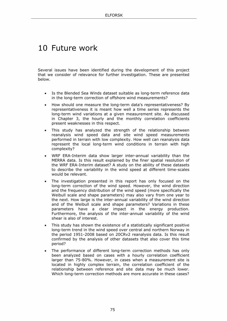
ELFORSK

75

10 Future work

Several issues have been identified during the development of this project that we consider of relevance for further investigation. These are presented below.

Is the Blended Sea Winds dataset suitable as long-term reference data in the long-term correction of offshore wind measurements?

How should one measure the long-term data's representativeness? By representativeness it is meant how well a time series represents the long-term wind variations at a given measurement site. As discussed in Chapter 3, the hourly and the monthly correlation coefficients present weaknesses in this respect.

This study has analyzed the strength of the relationship between reanalysis wind speed data and site wind speed measurements performed in terrain with low complexity. How well can reanalysis data represent the local long-term wind conditions in terrain with high complexity?

WRF ERA-Interim data show larger inter-annual variability than the MERRA data. Is this result explained by the finer spatial resolution of the WRF ERA-Interim dataset? A study on the ability of these datasets to describe the variability in the wind speed at different time-scales would be relevant.

The investigation presented in this report has only focused on the long-term correction of the wind speed. However, the wind direction and the frequency distribution of the wind speed (more specifically the Weibull scale and shape parameters) may also vary from one year to the next. How large is the inter-annual variability of the wind direction and of the Weibull scale and shape parameters? Variations in these parameters have a clear impact in the energy production. Furthermore, the analysis of the inter-annual variability of the wind shear is also of interest.

This study has shown the existence of a statistically significant positive long-term trend in the wind speed over central and northern Norway in the period 1951-2008 based on 20CRv2 reanalysis data. Is this result confirmed by the analysis of other datasets that also cover this time period?

The performance of different long-term correction methods has only been analyzed based on cases with a hourly correlation coefficient larger than 75-80%. However, in cases when a measurement site is located in highly complex terrain, the correlation coefficient of the relationship between reference and site data may be much lower. Which long-term correction methods are more accurate in these cases?

ELFORSK

76

11 Appendix - U&N method

11.1 Method description

The primary basis of the U&N method is the Q-Q method. This is a quantile method that consists in plotting quantile values of two datasets. The resultant plot is called the Q-Q plot. If the relation between the two datasets is linear, than the Q-Q plot shows a straight line. A simple example is the case of two datasets of the same size. In this case, to make the Q–Q plot, one orders each set in increasing order, then pairs off and plots the corresponding values. The Q-Q method ignores simultaneity, and focuses on the statistics of the datasets. The present version of the U&N method focuses on the wind direction and velocity. However, a relevant further development of this method would be to include stability. The methodology used seeks to capture the probability distribution of both the wind direction and the wind speed, as opposed to the majority of other long-term correction methods that focuses mainly on the direction distribution together with the mean value of the wind speed. The U&N method compares concurrent site and reference data, but unlike the majority of other LTC methods, the concurrency is only a starting point to ensure that the data represents the same time period.

11.1.1 Long-term direction distribution

The strength of the Q–Q methodology is also a weakness. When the concurrency for the wind direction is discarded, the direction conversion methodology will depend on a reference wind direction towards which the datasets are sorted. It is important that this reference wind direction represents the differences in the wind direction of the two sites as good as possible. To ensure this, the reference direction is chosen as the predominant wind direction at the reference station. For this direction, the corresponding median direction at site is found based on simultaneous data. The site wind direction time series is then corrected for the difference between these values. This synchronization of the endpoints is needed as the Q-Q method sorts the two datasets ascending independently. Note, that this difference is calculated based on simultaneous data but only for the predominant wind direction observations. This value is however applied to the entire direction series, even though the simultaneity of the entire series has not been taken into account. Based on the sorted wind direction time series for the site and the reference station, the direction difference is calculated for each 1° direction bin (Figure 11-1). The reference wind direction time series is then shifted by this difference to obtain the synthetic long-term time series of the site wind

ELFORSK

77

direction. The methodology used will ensure that the statistical properties of the site wind rose will be correctly represented in the resultant site long-term time series for the period of simultaneous data.

Figure 11-1. Example of the direction difference between a site time series and the corresponding reference time series.

11.1.2 Long-term wind speed distribution

As a result of the previous step, the site and reference wind speed time series are individually sorted by direction. The focus will now be on establishing the wind speed correction factors. The data is first divided into 24 direction sectors with equal number of elements in each sector. Since the sectors are defined based on equal amount of data, less predominant directions with few observations will be clustered into broader sectors, whereas the most frequent directions will form narrower sectors. This results in an improved accuracy of the long-term time series as compared to using the standard direction binning into 12 sectors with uniform width. A 12 sector version of the synthetic method is also available for comparison to other methods that are based on a 12 sector binning (different binning will cause some smoothing between the sectors).

ELFORSK

78

Regardless of the chosen binning method, the next step is to establish the wind speed relation between the site and the reference station for the given direction bin. Also here the wind speeds of the corresponding sectors at the site and the reference station are sorted individually to give a detailed wind speed relation. This relation is then applied to the long-term reference wind speed to obtain a synthetic long-term time series of the wind speed at the site. Figure 11-2 and Figure 11-3 show an example of the relation between the wind speeds at the site and the reference station for sectors 1 and 6, respectively. The relation for sector 1 is almost linear, whereas there is a kink at about 9 m/s for sector 6, reflecting a non-linear relation for this sector. A main advantage of this method is that non-linear properties are captured.

Figure 11-2. Relation between the site and the reference wind speeds for sector 1. The blue line indicates the extrapolation line for observations exceeding the values contained in the dataset.

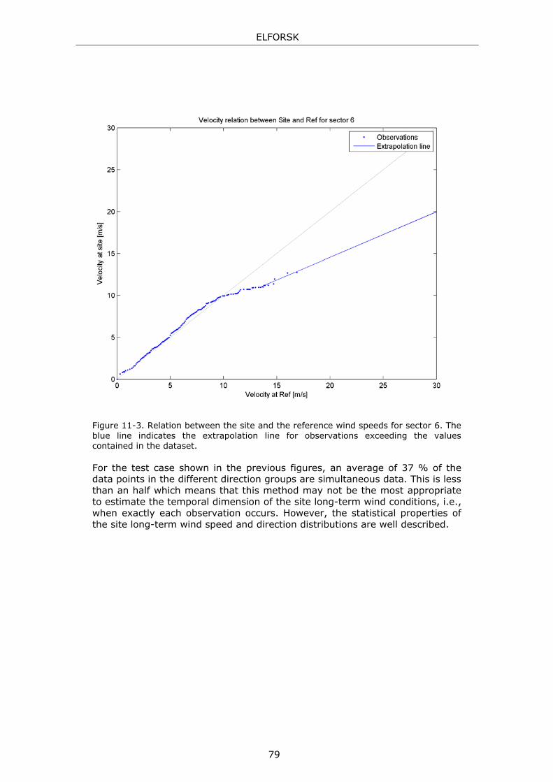
ELFORSK

79

Figure 11-3. Relation between the site and the reference wind speeds for sector 6. The blue line indicates the extrapolation line for observations exceeding the values contained in the dataset. For the test case shown in the previous figures, an average of 37 % of the data points in the different direction groups are simultaneous data. This is less than an half which means that this method may not be the most appropriate to estimate the temporal dimension of the site long-term wind conditions, i.e., when exactly each observation occurs. However, the statistical properties of the site long-term wind speed and direction distributions are well described.

ELFORSK

80

12 Bibliography

Albers, A., "Long term variation of wind potential: Are we moving into a low NAO-cycle period?", EWEA conference proceedings, 2004

Berrisford, P., Dee, D., Fielding, K., Fuentes, M., Kållberg, P., Kobayashi, S. and Uppala, S., "The ERA-Interim archive. Version 1.0.", ERA report series, 2009.

Compo, G.P., Whitaker, J. S., Sardeshmukh, P. D., Matsui, N., Allan, R. J., Yin, X., Gleason, B. E., Vose, R. S., Rutledge, G., Bessemoulin, P., Bronnimann, S., Brunet, M., Crouthamel, R. I., Grant, A. N., Groisman, P. Y., Jones, P. D., Kruk, M. C., Kruger, A. C., Marshall, G. J., Maugeri, M., Mok, H. Y., Nordli, O., Ross, T. F., Trigo, R. M., Wang, X. L., Woodruff, S. D., Worley, S. J., "The Twentieth Century Reanalysis Project", Quarterly J. Roy. Met. Soc., 2011.

CRAN, http://cran.r-project.org/, retrieved in 2012.

Dee, D. P., Uppala, S. M., Simmons, A. J., Berrisford, P., Poli, P., Kobayashi, S., Andrae, U., Balmaseda, M. A., Balsamo, G., Bauer, P., Bechtold, P., Beljaars, A. C. M., van de Berg, L., Bidlot, J., Bormann, N., Delsol, C., Dragani, R., Fuentes, M., Geer, A. J., Haimberger, L., Healy, S. B., Hersbach, H., Hólm, E. V., Isaksen, L., Kållberg, P., Köhler, M., Matricardi, M., McNally, A. P., Monge-Sanz, B. M., Morcette, J.-J., Park, B.-K., Peubey, C., de Rosnay, P., Tavolato, C., Thépaut, J.-N. and Vitart, F., "The ERA-Interim reanalysis: configuration and performance of the data assimilation system", Quart. J. R. Meteorol. Soc., 2011.

Ebita, A., Kobayashi, S., Ota, Y., Moriya, M., Kumabe, R., Onogi, K., Harada, Y., Yasui, S., Miyaoka, K., Takahashi, K., Kamahori, H., Kobayashi, C., Endo, H., Soma, M., Oikawa, Y. and Ishimizu, T., "The Japanese 55-year reanalysis "JRA-55": An interim report", SOLA, Vol. 7, 2011.

ECMWF, http://www.ecmwf.int/products/data/archive/descriptions/ei/index.html, retrieved in 2012.

EWEA, "Wind Energy - The Facts", 2009

Førland, E. J., Benestad, R. E., Flatøy, F., Hanssen-Bauer, I., Haugen, J E., Isaksen, K., Sorteberg, A. and Ådlandsvik, B., "Climate development in North Norway and the Svalbard region during 1900-2100", Norwegian Polar Institute, Report series no. 128, 2009

Garrad Hassan & Partners Ltd., "WindFarmer Theory Manual", 2011.

Garrett, P., ”Wind speed site tests come under scrutiny,” Wind Power Monthly, November 2011.

Gorsuch, R. L. and Lehmann, C. S., "Correlation coefficients: mean bias and confidence interval distortions", Journal of Methods and Measurement in the Social Sciences, Vol. 1, No. 2, 52-65, 2010.

ELFORSK

81

Harstveit, K., "Estimating long-term wind distribution from short-term data set using a reference station", EWEA conference proceedings, 2004.

Harstveit, K., Klinkert, R., Berge, E. and Tallhaug, L., "NORSEWInD - Long-term adjustments. Testing reference data sets and long-term adjustment methods", KVT/KH/2012/066, 2012.

Hasager, C. B., Barthelmie, R. J., Christiansen, M. B., Nielsen, M. B. and Pryor, S. C., "Quantifying offshore wind resources from satellite wind maps: Study area the north sea.", Wind Energy, 9, 2006.

JRA, http://www.jreap.org/indexe.html, retrieved in 2012.

Kalnay, E., Kanamitsu, M., Kistler, R., Collins, W., Deaven, D., Gandin, L., Iredell, M., Saha, S., White, G., Woollen, J., Zhu, Y., Leetmaa, A., Reynolds, B., Chelliah, M., Ebisuzaki, W., Higgins, W., Janowiak, J., Mo, K. C., Ropelewski, C., Wang, J., Jenne, R. and Joseph, D., "The NCEP/NCAR 40-year reanalysis project", Bull. Amer. Metor. Soc., 1996.

Kanamitsu, M., Ebisuzaki, W., Woollen, J., Yang, S.-K., Hnilo, J. J., Fiorino, M. and Potter, G. L., "NCEP-DOE AMIP-II Reanalysis (R-2) ", Bull. Amer. Metor. Soc., 2002.

Klemp, J., B., Skamarock, W. C., and Dudhia, J., "Conservative split-explicit time integration methods for the compressible nonhydrostatic equations", 2006, retrieved in 2012 from http://www.mmm.ucar.edu/individual/skamarock/wrf_equations_eulerian.pdf.

Liléo, S., and Petrik, O., "Investigation study on the use of NCEP/NCAR, MERRA and NCEP/CFSR reanalysis data in wind resource analysis", Scientific proceedings of the EWEA conference, 2011.

Lucchesi, R., "File Specification for MERRA products”, Global Modeling and Assimilation Office, 2008.

MDISC, http://disc.sci.gsfc.nasa.gov/daac-bin/FTPSubset.pl, retrieved in 2012.

Michalakes, J., Chen, S., Dudhia, J., Hart, L., Klemp, J., Middlecoff, J., and Skamarock, W., "Development of a Next Generation Regional Weather Research and Forecast Model", Developments in Teracomputing: Proceedings of the Ninth ECMWF Workshop on the Use of High Performance Computing in Meteorology, 2001.

NCDC, http://www.ncdc.noaa.gov/oa/rsad/air-sea/seawinds.html, retrieved in 2012a.

NCDC, http://www.ncdc.noaa.gov/oa/land.html, retrieved in 2012b.

Nygaard, T. A., "Estimating expected energy capture at potential wind turbines in Norway", Journal of Wind Engineering and Industrial Aerodynamics, 39, 1992.

Onogi, K., Tsutsui, J., Koide, H., Sakamoto, M., Kobayashi, S., Hatsushika, H., Matsumoto, T., Yamazaki, N., Kamahori, H., TAkahaski, K., Kadokura, N., Kamahori, H., Takahashi, K., Kadokura, S., Wada, K., Kato, K.,

ELFORSK

82

Oyama, R., Ose, T., Mannoji, N. and Taira, R., "The JRA-25 reanalysis", Journal of the Meteorological Society of Japan, Vol. 85, No. 3, 2007.

PSD, http://www.esrl.noaa.gov/psd/data/gridded/data.ncep.reanalysis.s

urface.html, retrieved in 2012.

RDA, http://dss.ucar.edu, retrieved in 2012

RSS, http://www.remss.com/, retrieved in 2012

Saha, S, Moorthi, S., Pan, H.-L., Wu, X.,Wang, J., Nadiga, S., Tripp, P., Kistler, R., Woolen, J., Behringer, D., Liu, H., Stokes, D., Grumbine, R., Gayno, G., Wang, J., Hou, Y.-T., Chuang, H.-Y., Juang, H.-M., Sela, J., Iredell, M., Treadon, R., Kleist, D., Van Delst, P., Keyser, D., Derber, J., Ek, M., Meng, J., Wei, H., Yang, R., Lord, S., Dool, H., Kumar, A., Wang, W., Long, C., Chelliah, M., Xue, Y., Huang, B., Schemm, J.-K., Ebisuzaki, W., Lin, R., Xie, P., Chen, M., Zhou, S., Higgins, W., Zou, C.-Z., Liu, Q., Chen, Y., Han, Y., Cucurull, L., Reynolds, R. W., Rutledge, G. and Goldberg, M., ”The NCEP Climate Forecast System Reanalysis,” Bull. Amer. Meteor. Soc., 2010, DOI: 10.1175/2010BAMS3001.1

Schär, C., ”Atmospheric data assimilation,” 2012, retrieved in 2012 from http://www.iac.ethz.ch/edu/courses/master/modules/numerical_modelling_of_weather_and_climate/05_DataAssim_FS12.pdf.

Skamarock, W. C., Klemp, J. B., Dudhia, J., Gill, D. O., Barker, D. M., Duda, M. G., Huang, X.-Y., Wang, W. and Powers, J. G., "A Description of the Advanced Research WRF Version 3", NCAR Technical Note NCAR/TN-475+STR, 2008.

Shea, D. J., Worley, S. J., Stern, I. R. and Hoar, T. J., ”An introduction to atmospheric and oceanographic datasets,” NCAR Technical Note, 1995.

Simmons, A., "Global numerical weather prediction and environmental monitoring: the present and future", ECMWF, 2004.

Tallhaug, L. and Nygaard, T. A., "The potential of wind energy in Sør-Trøndelag, Norway", EWEA conference proceedings, 1993.

Thomas, P., Cox, S. and Tindal A., "Long-term wind speed trends in northwestern Europe", EWEA conference proceedings, 2009.

Thøgersen, M. L., Nielsen, P., Bredelle, K., Svenningsen, L. and Jacobsen, T., "WindPRO/ONLINE, Remore sensing data and other data for download in WindPRO", EMD International A/S, 2010a.

Thøgersen, M. L., Nielsen, P., Sørensen, T. and Svenningsen, L. U., "MCP - Measure-Correlate-Predict, An Introduction to the MCP facilities in WindPRO", EMD International A/S, 2010b.

Thøgersen, M. L., Motta, M., Sørensen, T. and Nielsen, P., "Measure-Correlate-Predict Methods: Case Studies and Software Implementation", EWEA conference proceedings, 2007.

Trenberth, K. E., "Atmospheric reanalyses: a major resource for climate services", Group on Earth Observations (GEO), 2010.

ELFORSK

83

Uppala, S. M., Kållberg, P. W., Simmons, A. J., Andrae, U., da Costa Bechtold, V., Fiorino, M., Gibson, J. K., Haseler, J., Hernandez, A., Kelly, G. A., Li, X., Onogi, K., Saarinen, S., Sokka, N., Allan, R. P., Andersson, E., Arpe, K., Balmaseda, M. A., Beljaars, A. C. M., van de Berg, L., Bidlot, J., Bormann, N., Caires, S., Chevallier, F., Dethof, A., Dragosavac, M., Fisher, M., Fuentes, M., Hagemann, S., Hólm, E., Hoskins, B. J., Isaksen, L., Janssen, P. A. E. M., Jenne, R., McNally, A. P., Mahfouf, J.-F., Morcrette, J.-J., Rayner, N. A., Saunders, R. W., Simon, P., Sterl, A., Trenberth, K. E., Untch, A., Vasiljevic, D., Viterbo, P. and Woollen, J., "The ERA-40 re-analysis.", Quart. J. R. Meteorol. Soc., 131, 2961-3012, 2005.

Verbesselt, J., Hyndman, R., Newnham, G. and Culvenor, D., "Detecting trend and seasonal changes in satellite image time series", Remote Sensing of Environment, 2009.

Wern, L. and Bärring, L., "Sveriges vindlimat 1901-2008. Analys av förändring i geostrofisk vind", Meteorologi Nr 138/2009, SMHI, 2009.

Wikipedia Correlation, http://en.wikipedia.org/wiki/Correlation_and_dependence, retrieved in 2012.

Wikipedia Quantile, http://en.wikipedia.org/wiki/Quantile, retrieved in 2012.

Wikipedia Statistical significance, http://en.wikipedia.org/wiki/Statistical_significance, retrieved in 2012.

WRF, http://www.wrfmodel.org/, retrieved in 2012.

ELFORSK

84