long-term dependence characteristics of european stock indices

1

Long-Term Dependence Characteristics

Of European Stock Indices

Joanna M. Lipka

Department of Finance, BSA 420 Kent State University, Kent, OH 44242-0001

330-672-1208; [email protected]

Cornelis A. Los*

Department of Finance, BSA 416 Kent State University, Kent, OH 44242-0001

330-672-1207; [email protected]

July 2003

The authors would like to thank Rossitsa Yalamova for assisting with the computation of the wavelet statistics. The authors remain fully responsible for this paper’s contents. * Corresponding author

2

Long-Term Dependence Characteristics

Of European Stock Indices

Abstract

This paper measures the degrees of persistence of the daily returns of eight European stock market indices, after their lack of ergodicity and stationarity has been established. The proper identification of the nature of the persistence of financial time series forms a crucial step in deciding what kind of diffusion modeling of such series might provide invariant results. Our results indicate that ergodicity and stationarity are very difficult to establish with only daily observations of market indexes and thus various price diffusion models cannot be successfully identified. However, the measured degrees of persistence point to the existence of long-term dependencies, most likely of a nonlinear nature. Global Hurst exponents, computed from wavelet multi-resolution analysis, measure the long-term dependence of the data series. The FTSE turns out to be an ultra-efficient market with abnormally fast mean-reversion, faster than theoretically postulated by a Geometric Brownian Motion. But the various measurement methodologies produce non-unique empirical results and thus it is very difficult to obtain definite conclusions regarding the presence or absence of long-term dependence phenomena based on the global Hurst exponents. Although it is our judgment from these daily data that most stock markets in Europe appear to be anti-persistent, more powerful methods, such as the computation of the multifractal spectra of financial time series may be required. Still, we demonstrate that the visualization of the wavelet resonance coefficients and their power spectra, in the form of localized scalograms and averaged scalegrams, forcefully assists with the detection and measurement of several nonlinear types of market price diffusion.

3

1. Persistence in Financial Price Series For a long time, financial researchers have struggled with the identification of properly

specified econometric and time series models that can capture the dynamic dependence in

financial time series. The most popular models that account for lagged observations are the

family of ARIMA models and the family of GARCH models. Some models from these families

have become extremely popular among technical analysts due to their ability to capture short-

term dependence. Unfortunately, these, often linear, models are criticized for not being able to

model long-term dependence too well and for requiring (and often presuming) Gaussian

distribution characteristics for the residuals.

Loretan and Phillips (1994) recognize that distribution characteristics of time series often

vary over time. Cochrane (1988) already pointed out several weaknesses of the ARIMA models

and suggested a measure for long-term dependence, like unit root integration A(1), because of

the presence of approximate common factors in the AR and MA polynomials. A very common

and easily recognizable weakness of the ARIMA and GARCH models is the requirement for the

modeled residual series to be stationary. Although one can achieve apparent wide-sense

stationarity of the financial series after several adjusted differencing transformations, it has

become clear that such adjusted differencing cannot remove the time dependence in the series

between far-distant observations: the remaining auto-covariance functions (ACFs) of the squared

errors just don’t die out. This feature has also been observed in certain hydrological studies of

long-range rivers and has been called the Hurst effect (Mandelbrot and Van Ness, 1968).

It has again come into research focus in the past decade. Recently, there a number of

studies have appeared devoted to measuring such persistence phenomena in various financial

data series using newer measurement technologies used in signal processing. A short discussion

4

on persistence is provided, for example, in Mills (1999). Mandelbrot (1969, 1972) introduced

the concept of the long-term persistence in the study of time series of economic and financial

prices. With Fama he researched the resulting non-Gaussian distributions of financial prices.

Once the concept of long-term memory in prices was accepted in the late 1970s, financial

researchers searched for models that could properly identify such long-term dependence

behavior. Hosking (1981) and Granger and Joyeux (1980) built on the prevalence of the well-

known ARIMA models and proposed fractionally integrated ARMA models to measure long-

term dependence. These models are more recently discussed in greater detail in Beran (1992),

Baillie (1996) and Robinson (1994). Empirical studies of long-term dependence often rely on

the study of Geweke and Porter-Hudak (1983), who proposed a method for the calculation of

Hosking’s fractional differencing parameter d.

The finding of long-term dependence in financial data might be in contradiction with the

Efficient Markets Hypothesis of Fama (1970), which is based on the assumption of martingale

behavior of financial market prices. The martingale theory requires an invariant stationarity and

independence of the innovations of the historical price information sets, but it is difficult to show

that this requirement is met either in weak form or, even less so, in strong form. Peters’ work

(1994) on the Fractional Market Hypothesis is an application of long-term dependence concept

that is broader and encompasses Fama’s theory of market efficiency.

The objective of this paper is to identify the dynamic diffusion models of several

European equity indexes. This is done primarily to demonstrate that even though in the literature

on econometric modeling one can find various models that fit financial data apparently well, one

cannot fully rely on the conclusions about the properness of the identification of these models.

For example, conventional econometric and time series modeling emphasizes only the

5

measurement of the first two moments of the residuals, but ignores the measurement of the

higher moments. Or, in frequency terms, it ignores the whole power spectrum of the

innovations. Caution with respect to these “statistically estimated” models is therefore highly

recommended, because, when these models are estimated. It is more often than not presumed

that the data meet the assumptions of the theoretical models, even though the data show glaring

discrepancies from those basic assumptions. Sometimes it is now even admitted that the data do

not meet the assumptions of the theoretical models, but despite that admission the models are

still being “estimated” and the results used with a confidence that is scientifically unwarranted

(Los, 2001).

To pursue the objective of this paper and to shed some light on such analytical

inconsistencies, we’ll try to answer several questions about the dynamic character of stock

market index prices for several European countries. Answering these questions is crucial for

performing further econometric and time series analysis of the daily price traces, which are used

for the valuation of and hedging by derivatives and, thus, for serious portfolio risk management.

These questions are:

1. Are the pricing series or their innovations ergodic?

2. Is the pricing series or their innovations stationary? And if so, are they strict or wide-

sense stationary?

3. Do the pricing series, after proper Taylor expansion type differencing, exhibit

independence, short-term dependence or long-term dependence?

4. If the pricing series exhibit long-term dependence, are they persistent or anti-persistent?

5. What are the theoretical benchmark models for the analyzed pricing series?

6

6. How far do the empirically identified dynamic price diffusion models deviate from

theoretical benchmark models?

7. Can the identified pricing models help market traders to earn abnormal returns?

In the context of this paper, a more detailed discussion of the approach to question 4

might be worthy some more elaboration, because of its unfamiliarity among financial analysts

and econometric researchers. We measure the degree of global persistence by computing the

Hurst exponent from the wavelet multi-resolution analysis (MRA) developed by signal

processing engineers, such as Mallat (1989). MRA is a powerful technique that allows one to

simultaneously analyze time series in both time and frequency domains. This feature is a simple

way to identify time series data, since it also allows for the measurement and visualization of

nonlinear dependencies, and thus of dependencies other than the usual collinearities between

integer lags, which only measure simple linear dependencies.

A scalogram, which is a color-coding visualization of the measured wavelet resonance

coefficients, i.e., of the squared correlation coefficients between the time series and the chosen

wavelet bases, allows one to immediately detect shocks in financial markets and their localized

frequency strength or power or risk.

The average of such scalograms over time, that can be graphically represented by the

logarithm of the average power spectrum of the financial time series, or a scalegram, allows one

to investigate the autocorrelation function of the financial time series in the conventional

Fourier-type frequency dimension and thus to identify possible (certain) periodicities or

cyclicities (= uncertain periodicities) in the stock indexes. Such periodicities cannot be easily

viewed when the statistical methodologies of classical time series analysis are used.

7

This paper is organized as follows: section 2 contains a short review of the long-term

dependence literature; section 3 presents the details of the stock market index data; and section 4

discusses the methodologies used in this paper, together with the measured empirical results.

Finally, section 5 draws some tentative conclusions.

2. Long-Term Dependence

One of the first finance researchers who formally recognized long-term persistence in

financial economic data was Mandelbrot (1969, 1972). By doing so, he launched a search for the

proper model identification to account for this phenomenon. Granger and Joyeux (1980), and

Hosking (1981) developed a method of determining long-term dependence with fractionally

integrated ARMA, or ARFIMA models. Geweke and Porter-Hudak (1983) proposed calculating

the differencing parameter d that allows one to determine the level of long-term dependence.

Beran (1992), Baillie (1996) and Robinson (1994) review such models of long-term dependence

and their applications. Ding, Granger, and Engle (1993) focus on the detection of the long-term

memory process in second moments, which are of importance to financial risk analysis and

management. Baillie, Bollerslev, and Mikkelsen (1996) capture long-term dependence with their

newly introduced class of fractionally integrated generalized autoregressive conditionally

heteroskedastic (FIGARCH) processes by applying it to daily Deutschmark-U.S. dollar exchange

rates. Bollerslev and Mikkelsen (1996) use the FIGARCH process to model financial market

volatility, in particular in the foreign exchange markets, and assert, not completely convincingly,

that a mean-reverting fractionally integrated process is superior in characterizing the volatility

than any other model. In a slightly different approach, Crato and de Lima (1994) find long-

memory or persistent stochastic volatility in high-frequency stock market data.

8

Thus far, the identification results, regarding the degree of long-term dependence or

memory in the analyzed data, appear to depend very much on the analytic methodology used and

therefore calls into question how and if it really can be identified by the existing methodologies

and technologies. For example, Green and Fielitz (1977) and Aydogan and Booth (1988) apply

in their studies the R/S (range-over-scale) metric of Hurst (1951) to test the long-term

dependence in common stock return. But then Lo (1991) uses the modified rescaled range

statistic for value and equal weighted CRSP index returns and finds that although the original

Hurst rescaled range statistic detects the existence of the long-memory in the data, his modified

Hurst statistic rejects such long-term memory. Moreover, Lo also cannot find the long-term

dependence in annual returns for a long period from 1872 until 1986. We suspect that Lo

focused on only one type of long-term dependence-persistence and could not find it, because

these series represent the other type of long-term dependence: anti-persistence. If so, the

research question should be reformulated and the technology adjusted to enable the detection of

both types of long – term dependence. Also, Lo’s modification incorporates only the linear

research technology of collinearity analysis, which, per definition, cannot detect nonlinear long-

term dependencies. It is of importance to emphasize that collinearity analysis can only detect

linear dependencies in the data. It cannot detect nonlinear dependencies. We suspect that

nonlinear dependencies are more prevalent in the data than linear dependencies.

The detection of long-term dependence processes has crucial implications for the

measurement of the efficiency of financial markets. If long-term dependence is confirmed in

asset prices, then one can have a viable suspicion about the existence of even the weakest form

of efficiency, not to mention of other forms of financial market efficiency. Los (2000) and by

Sadique and Silvapulle (2001) brought this issue into focus. Los (2000) used nonparametric

9

efficiency tests of markets of Hong Kong, Indonesia, Malaysia, Singapore, Taiwan, and Thailand

and rejected their efficiency on the basis of lack of stationarity and independence of the time

series innovations. Sadique and Silvapulle looked specifically for long memory process in the

stock market returns of Japan, Korea, New Zealand, Malaysia, Singapore, the USA and

Australia, with the help of classical and modified rescaled range tests, the semi-parametric test

proposed by Geweke and Porter-Hudak, the frequency domain score test proposed by Robinson

and its time-domain counterpart derived by Silvapulle. Their study finds long-term dependence

in stock market returns in Korea, Malaysia, Singapore and New Zealand. The results of Los and

of Sadique and Silvapulle are in contradiction with the results of Cheung (1995), who did not

find a persuasive support for the stock returns of eighteen countries of Asia, Europe, and North

America using the classical techniques.

Given the lack of agreement on the existence of long-term memory process in stock

returns, it is important to study this phenomenon further using more powerful methodologies and

technologies. A significant contribution to such a more and more influential study of the

persistence in financial data is Los (2003), who, in great detail and in language understandable to

financial and economic researchers, reviews the currently available time-frequency signal

processing methodologies and technologies to detect and measure long-term dependence,

including the measurement not only of homogeneous or global Hurst exponents, but also of

multifractal spectra of Lipschitz alphas. Recently, Mandelbrot contended that financial time-

series probably are multifractal, or more precisely, can be modeled by Geometric Brownian

Motion in multifractal time (Mandelbrot, 1997).

10

3. Data

The data used in this paper are daily deviations on eight European stock market indices

and their various simple transformations. Detailed information for the indices is presented in

Table 1 and in Table 2. The time period for the series varies from index to index due to data

availability. All the series were taken from the “Yahoo, Finance!” website and therefore are

freely available for further inspection and for replication of the results of this paper.

We analyze various transformations of the stock market indices: the index levels, X(t),

logarithms of index levels, ln{X(t)}, differenced index levels D[X(t)], differenced logarithm of

index levels, D[ln{X(t)}], which are the stock market returns, and differenced returns, D[x(t)].

These transformations of index levels and their returns are analyzed to find out whether the

applied transformations allow one to find desirable properties of the data, such as stationarity and

ergodicity. We also provide graphs supporting the conclusions of our study. The graphs

included in this paper are only for the FTSE series, due to space limitations. The graphs for all

other data series studied in this paper are available upon request.

4. Methodology and Empirical Identification Results A) Ergodicity, Stationarity, and Independence

Ergodicity is defined by Terence C. Mills (1999, p. 9) as follows: “… the process is

ergodic, which roughly means that the sample moments for finite stretches of the realization

approach their population counterparts as the length of the realization becomes infinite.” Mills

remarks that it is impossible to test for the ergodicity of time series using only one realization

and thus he assumes that all time series have this property. That is a very strong but tenuous

assumption. Obviously, one cannot have more than one historical realization of any time series.

11

However, one can use time-ordered sample drawings of data from the available historical time

series as substitutes for various length increasing realizations of a given population or infinite

sample. Thus, moments for the five time series for each index using time windows of increasing

size are computed and then these computed moments are plotted against their window length.

One can then visually inspect whether the plots gradually converge to a flat line, which would

suggest ergodicity of the time series.

In neither of our data series, we observe such gradual convergence to a flat time line.

Several sharp discontinuities and shifts occur, which is an indication of fractality in the time

series, and no convergence points appear to exist. Thus, visually it is reasonable to conclude that

these series are not ergodic. Of course, it is an empirical scientific question, what realization is

long enough to decide that the estimated moments can be relied on to make conclusions about

ergodic property of a time series. Therefore several window sizes were tried. None provides

results that even remotely could suggest ergodicity of these stock market time series. As an

example of the increasing-window methodology, the first four moments of the analyzed FTSE in

are plotted in Figure 2. This lack of visual ergodicity suggests that the usual procedure of using

time moments as substitutes for ensemble moments is empirically severely flawed (or may we

even conclude: it is visually falsified?).

A time series is said to be strictly stationary if the joint distribution of any set of

n observations Xt1, Xt2, …, Xtn is the same as the joint distribution of Xt1+k, Xt2+k, …, Xtn+k for all n

and k. Strict stationarity is difficult to observe in financial time series data, because we would

have to compute an infinite set of moments, since for an unknown distribution it is unknown how

many moments exist. Thus, the strict stationarity assumption is often relaxed to weak or wide

sense stationarity. A time series is said to be weakly stationary if its first moment or mean is

12

constant and its second moment or auto-covariance function (ACF) depends only on the time

lags. If you normalize the ACF on the time lags you would see one constant standard definition

or a horizontal time line over time in the normalized ACF plot.

In order to test for wide sense stationarity with an expansion to third and fourth moments,

rolling windows are computed for the first four moments of all stock market indices and their

transformations. As a representative example of the plots for these four rolling-window

moments, the moments for FTSE are plotted in Figure 3. In neither case constant moments are

observed. Again sharp shifts occur in the rolling window moments, an indication of the possible

fractality of the time series. Thus, we conclude that our series are neither strict-sense nor wide-

sense stationary.

The elements of a time series are independent if the autocorrelation function of this series

equals one for the lag equal to zero and zero for any lag different from zero. A time series is

long-term dependent if the autocorrelation function for the series decays at some hyperbolic rate.

The decay at a hyperbolic rate is much slower than the decay at the geometric rate. To

investigate the nature of the dependence of the time series, one can thus visually inspect the

autocorrelation function of each of the five series. The autocorrelation functions, or ACFs of the

five stock market indices, and their transformations were computed and inspected up to 200 lags.

Table 3 shows that the behavior of the autocorrelation function varies for each of the five

series. For prices, logarithms of prices, and differences of returns, one can easily detect short-

term dependence, because the autocorrelation function takes significant values for initial lags.

For example, for one lag the absolute values of the ACFs vary from 0.441 up to 0.999 for these

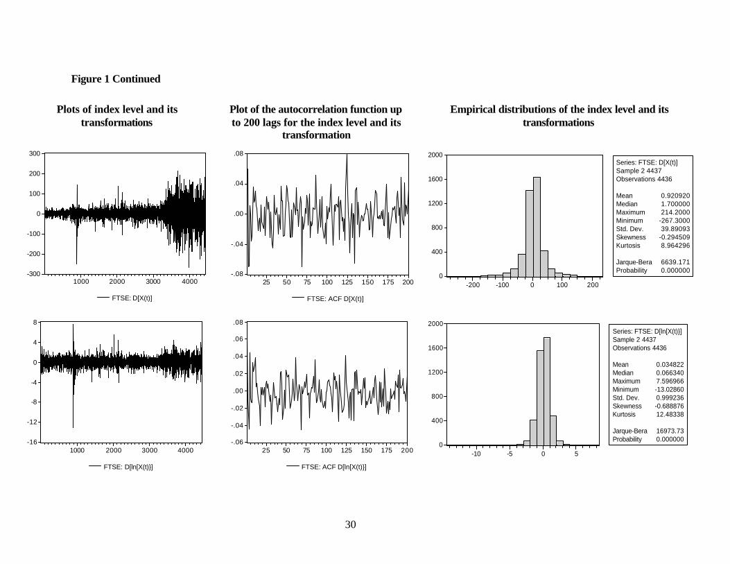
series. ACFs for the differences of prices and for returns are much smaller than for other series

and their absolute values vary between 0.036 and 0.176. For the price levels and for the

13

logarithmic transformations of prices, the autocorrelation function has a clear pattern and slowly

dies off, thereby suggesting the existence of long-term dependence.

An empirical question is for how many lags the autocorrelation function should be

different from zero in order to undoubtedly admit the long-term dependence. Assuming that 200

days is a long enough period to determine the long-term dependence for our daily data, large

values for ACFs for 200 lags for prices and logarithms of prices suggest that one can detect long-

term memory in these series. For other transformations of prices, like for the differences of

prices, returns, and differences of returns, there are no clear patterns in the autocorrelation

functions. The plots oscillate around zero without visible decline in the amplitudes of the ACF.

The nature of the ACF functions for the studied series is indicated in Table 4, which

reports maximum, minimum, and the difference for minimum and maximum values for the

various ACFs. The minimum and maximum values constitute a bandwidth for the ACF.

Because the autocorrelation function is a decreasing function for prices and for logarithms of

prices for the first 200 lags, small values of the difference between the maximum and minimum

for ACFs suggest a stronger long-term dependence, and large values for the difference between

maximum and minimum for ACFs suggest a weaker long-term dependence. Based on this, one

can see that the strongest long-term dependence in prices occurs for the FTSE and the weakest

long-term dependence for prices and for logarithm of prices occurs for the SMSI. The

differences between maximum and minimum for ACFs for the differences of prices, returns, and

differences of returns are very small. However, they remain different from zero. Because the

plot for these series is rough with visible positive and negative spikes occurring at different lags,

this suggests that these series retain weak long-term memory. Examples of plots of the

autocorrelation functions are provided in Figure 1 and Figures 4 and 5.

14

B) Persistence

Based on the visual inspection of the ACF function, the series appear to be long-term

dependent, and therefore can be better represented by Fractal Brownian Motion (FBM) then by

Geometric Brownian Motion. For the model of Fractal Brownian Motion, the Hurst exponents,

H, are computed for all the series, in order to determine the degree if their long-term dependence.

The three manifestations of the long-term dependence are anti-persistence, when 0 < H < 0.5,

white (independent) noise when H = 0.5, and persistence when 0.5 < H < 1.

We computed the Hurst exponent by seven different method and summarized the results

in Tables 5 and 6: (1) R/S Analysis Method (R/S), (2) Power-Spectral Analysis Method (P-S),

(3) Roughness-Length Relationship Method (R-L), and (4) Variogram Method (V), (5) the

method proposed by developers of the IDL Wavelet Toolkit software1, (6) the method developed

by Veitch and Arby of the University of Melbourne2, and (7) the method proposed by developers

of FracLab software3. Table 7 reports more extensive results obtained from a procedure

developed by Veitch and Arby.

Based on the calculated Hurst exponents, we find that stock market index series might be

either persistent, P, or anti-persistent, AP, or white noise. It depends on the particular stock

market. In order to draw any general conclusion about the data, one might decide that the series

has a given property, if the majority of the proposed methods of analysis identify the given

property. Thus, based on the results in Table 6, the ATX, CAC 40, DAX, IBEX, SMSI, and

FTSE prices appear persistent. In case of KFX and TOTX, however, the results remain

1 The IDL Wavelet Toolkit software was developed by Research Systems, a Kodak Company, and is available on the http://ion.researchsystems.com/IONScript/wavelet/ website 2 The code for the procedure and the description of the procedure is available on the following website http://www.cubinlab.ee.mu.oz.au/~darryl/secondorder_code.html 3 FracLab software is available for free on the following website http://fractales.inria.fr/index.php?page=fraclab

15

inconclusive. If one requires that all methods allow for the same unique conclusion about the

nature of long-term dependence, for stock market in general, then the empirical results remain

inconclusive. It would clearly be of no added value to require some sort of “significance”

criterion, since each of the methods has different residual noise characteristics, because of the

different projections involved. Thus, our conclusion is that the degree of the measured

persistence depends on the particular stock market. Some stock markets are anti-persistent and

are thus ultra-efficient. Some stock markets show independent innovations, and thus are

efficient in the traditional sense. But some stock markets are persistent and thus inefficient and

even dangerous: long periods of calmness in pricing may be disrupted by sudden and large

discontinuities and drawdowns. Such differences in the degrees of persistence between the

various financial markets are probably caused by the differences in their institutional

organization.

Because in modeling of financial series the idea has always been accepted to test whether

well-established models can fit the data, this paper also examines whether the European indexes

can be proxied by some theoretical models available in the theoretical financial literature. The

theoretical models that can be used to compare with the empirical time series are the random

walk model, the Geometric Brownian Motion and the Fractional Brownian Motion. These

models are defined in the following way (Los, 2003):

Definition 1: A random walk model is a particular wide sense Markov or unit root

process of the original variables with independent innovations:

X(t) – X(t-1) = (1 – L)X(t) = e(t), where e(t) ~ i.i.d.(0, se2) and L is the one – period lag

operator.

16

Definition 2: A geometric Brownian motion is a random walk of the natural logarithm of

the original process. Thus lnX(t) –lnX(t-1) = x(t) are the rates of return and for Brownian

motion:

?x(t) = x(t) – x(t-1) = (1 – L)x(t) = e(t), where e(t) ~ i.i.d. (0, s e2)

Definition 3: Fractional Brownian Motion (FBM) is defined by the fractionally

differenced time series (1 – L)dx(t) = e(t), d ? ( -0.5, 0.5) with e(t) ~ i.i.d.(0, s e2).

Based on the rolling window test of the first four moments and based on the ACF

function, the first differences of prices, returns, which are first differences of logarithms of

prices, and the first differences of returns are not identically and independently distributed.

Thus, prices, logarithms of prices and returns are clearly not processes integrated from or driven

by white noise and the random walk model is immediately falsified.

To compare our series with the geometric Brownian motion, the ACF function for the

analyzed series is compared with the correlations of geometric Brownian motion. (ACF

comparison for FTSE series is provided in Figure 4). In almost all cases, the correlations of

geometric Brownian motion substantially differ from the calculated ACFs for the original series.

Thus, we also reject the geometric Brownian motion as a good model to fit the analyzed series.

To compare the empirical series with the theoretical FBM, one can compare the

autocorrelation function of the series with the FBM based autocorrelation function that is given

by the formula: ?(t) = t? G(t) for ? ? [-1, 0), or ?(t) = -t ? G(t) for ? ? [-2, -1). In this formula t is

time lag, G(t) is a slowly varying function at infinity (like a constant or a proportion of the time

lag t, and the exponent ? is related to the Hurst exponent by the following relationship

? = 2H – 2. Because we obtain different Hurst exponents with different estimation methods, one

17

needs to compute different ACFs functions with different ?s and then to compare the obtained

ACFs functions with ACFs of the original series. We suspected that FBM based ACFs are the

closest to the original ACFs. Thus we computed ACFs for the theoretical FBMs for all series

using the empirical ?s, but even these ACFs still do not approximate well the original ACFs.

(The ACF comparison for FTSE series is provided in Figure 5)

The models that most likely can be used to identify abnormal stock market returns are

those models which represent the persistence of the time series, that is models for which 0.5 < H

< 1.0. The series that appear to be anti-persistent with 0 < H < 0.5 are abnormally fast mean –

reverting and will not generate abnormally high returns, since those markets are ultra-efficient.

C) Persistence and Wavelet MRA Plots

Examples of the scalogram and scalegram results of the wavelet MRA are plotted in

Figure 6. A scalogram measures all power spectra localized in time and frequency (=1/scale)

domains at various scales and for various times. The wavelet resonance coefficients are

computed by Mallat’s (1989) wavelet MRA with the use of Morlet-6 wavelet4. A scalogram,

which is a visualization of the colorized wavelet resonance coefficients, allows one to identify

the precise timing and power of the innovations or shocks occurring in the markets. Scalegrams

are averaged based on wavelet bases scalograms and thus comparable to Fourier spectra based on

trigonometric bases. They help to detect the institutional periodicities or, more precisely, the

aperiodic cyclicities (= uncertain “periodicities”) of the financial markets, which cannot be easily

identified by the static ergodicity-based methodologies. Scalegrams also assist with the

identification of the global or homogeneous Hurst exponent for each time series and can

4 Often wavelets with six or more non-vanishing moments produce similar results. Less non-vanishing moments tend to obfuscate the details of the analysis because the wavelet basis is too regular. The more non-vanishing moments, the more irregular the wavelet is. The less non-vanishing moments, the shorter a wavelet is. E.g., the Gaussian wavelet has only two non-vanishing moments.

18

determine if the residuals are, indeed, white noise. The discussed scalograms and scalegrams in

this paper are computed with the help of software available on the following website:

http://ion.researchsystems.com/IONScript/wavelet.

There are three parts in each plot in Figure 3. Part (a) is the plot of original time series

and the type of wavelet used to analyze the time series, c.q. the Morlet-6 wavelet, often used for

the analysis of meteorological and environmental time series, such as the El Niño effect, or the

level of CO2. Part (b) is the scalogram, which is the color-coded plot of the magnitude of the

wavelet resonance coefficients. Finally, part (c) is the scalegram, which is the logarithm of the

power spectrum or Fourier transform of the series’ autocorrelation function (ACF).

On the basis of the price and return time series of FTSE index, one can see in Figure 7

that there are numerous spikes in the processes, which are consistent with sudden changes in the

stock market prices. Figure 7 shows that the most significant price changes in the FTSE have

occurred in October 1987, October 1989, April 1992, September 1992, October 1998, January

2000, and September 2001. For example, the sudden decline in the FTSE stock index in

October, 1987 followed the crash in the US stock markets (black Monday), caused by rapidly

rising of short term US interest rates, followed by rapidly rising long-term US interest rates, a

weakening US dollar, deteriorating US current account deficit, unjustifiably high domestic price-

earnings-ratios, very low dividend yields, and, most likely, too optimistic investor sentiment.

In terms of the wavelet analysis, stock market crashes can be easily detected by sudden

spikes in power, or singularities, indicated in the scalogram by a steep upward migration of blue,

green to red color. In October 1987, on the scalogram, one sees the burst of higher power

through all frequencies for both stock market prices and returns, spreading from the high

frequencies (at the top) to the low frequencies (at the bottom). The scalegram makes it easy to

19

calculate the Hurst exponent from slope of the line fitted to the scalegram, which is 2H+2 for the

price indices. The Hurst exponents calculated from the slope of the line fitted to the scalegram

are reported in Table 5 under the title IDL Wavelet Toolkit. In case of the FTSE, the Hurst

exponent is 0.33, indicating anti-persistence in the FTSE stock market returns data and definitely

not consistent with a long memory or persistent process of H > 0.5. It indicates that the FTSE is

an ultra-efficient market with abnormally fast mean – reversion, faster than theoretically

postulated by a Geometric Brownian Motion (which has H = 0.5).

V. Conclusions

This paper attempts to identify the ergodicity, stationarity, independence, and persistence

of the eight European index prices and their transforms, or the lack thereof. We find that the

analyzed data are far from being either ergodic, or stationary or independent. Thus, such series

cannot be modeled with ARIMA or GARCH family models that assume stationarity of the final

residual series. The stock market prices and their returns and their various transformations are

then compared with theoretical benchmark models, which are white (independent) noise (which

integrates to Brown noise), Geometric Brownian Motion, and Fractional Brownian Motions.

Even though some series appear to be fitted quite well by the white noise residual model (based

on the computed global Hurst exponent), the estimated ACFs contradict often this finding. This

demonstrates that the indiscriminate use of the global, homogeneous Hurst exponent computed

from the average power spectrum (or Fourier transform of the ACF) is also not completely

substantiated.

It remains an empirical scientific question which theoretical model is better for modeling

of the original financial market series. The Fractional Brownian Motion is more general and

20

encompasses the Geometric Brownian Motion. But also the Fractional Brownian Motion cannot

capture all the empirically observed intricacies, such as “cyclicities” or “uncertain and time-

varying periodicities” and the extremely valued power spikes observable in the power spectra of

the stock market returns, as was originally suggested by Mandelbrot. Finally, the question

should be raised whether such models can be used to earn abnormal stock market returns, in

particular when persistence is observed. The methods thus far suggested in the literature appear

not to lead to unique scientific conclusions regarding stock market returns in general. For

example, not all European stock markets are conventionally efficient, but some appear to be anti-

persistent or ultra- efficient, such as the FTSE, and some are persistent and inefficient.

The more important question for regulators and risk managers is thus which of the other

European stock market indices are persistent and thus inefficient and which can therefore

produce abnormal returns? By strictly focusing on long-term memory, i.e., persistence, and by

not allowing for the possibility of anti-persistence, many research analysts have been guided

themselves into blind alleys, since most of the European stock market indices appear to exhibit

anti-persistent behavior. But the methods currently suggested in the literature lead to non-unique

overall results. There exists no general stock market model. The various stock markets clearly

differ in their degrees of persistence. It is most disturbing is that the various research

methodologies do not yet lead to unique model identification results even for the same market.

However, this paper does find that visualization of the time-frequency spectra by wavelet

scalograms is a useful way to visualize the important localized characteristics of the financial

time series. Of course, scalegrams and spectrograms are also based on computed averages, be it

based on wavelets or Fourier transforms in the scale, respectively frequency domains and thus on

the ergodicity in the frequency domain. Accordingly they also tend to obscure the important and

21

not easily modeled, localized risk and time-variant higher moment phenomena, which are clearly

observable in scalograms. This suggests that researchers must pay more attention to the changes

in frequencies of the time series over time

22

References Baillie, R. T., ‘Long memory processes and fractional integration in econometrics’, Journal of

Econometrics, Vol. 73, 1996, pp. 5-59. Baillie, R. T., Bollerslev, T., and Mikkelsen, H. O., ‘Fractionally integrated generalized

autoregressive conditional heteroskedasticity’, Journal of Econometrics, Vol. 74, 1996, pp. 3-28.

Beran, J. A., ‘Statistical methods for data with long-range dependence’, Statistical Science, Vol.

7, 1992, pp. 404 – 27. Cheung, Y. W., ‘A search for long memory in international stock market returns’, Journal of

International Money and Finance, Vol. 14, 1995, pp. 597-615. Cochrane, J. H., , ‘How big is the random walk in GNP?’, Journal of Political Economy, Vol.

86, 1988, pp. 893-920. Crato, N. and de Lima, P. J. F., ‘Long-range dependence in the conditional variance of stock

returns’, Economic Letters, Vol. 45, 1994, pp. 281-285. Ding, Z., Granger, C. W. J., and Engle, R. F., ‘A long memory property of stock returns and a

new model’, Journal of Empirical Finance, Vol. 1, 1993, pp. 83-106. Fama, E. F., ‘Efficient capital markets: A review of theory and empirical work’, Journal of

Finance, Vol. 25, 1970, pp. 383-417. Geweke, J. and Porter-Hudak, S., ‘The estimation of and application of long memory time series

models’, Journal of Time Series Analysis, Vol. 4, 1983, pp. 221-238. Granger, C. W. J. and Joyeux, R., ‘An introduction to long memory time series models and

fractional differencing’, Journal of Time Series Analysis, Vol. 1, 1980, pp. 15 – 29. Greene, M. and Fielitz, B., ‘Long-term dependence in common stock returns’, Journal of

Financial Economics, Vol. 4, 1977, pp. 339-349. Hosking, J. R. M., ‘Fractional Differencing’, Biometrika, Vol. 68, 1981, pp. 165-76. Hurst, H. E., ‘Long-term storage capacity of reservoirs’, Transactions of the American Society of

Civil Engineers, Vol. 1, 1951, pp. 519 – 543. Lo, A. W., ‘Long-term-memory in stock market prices,’ Econometrica, Vol. 59, 1991, pp. 1279-

1313. Loretan, M. and Phillips, P. C., ‘Testing the covariance stationarity of heavy-tailed time series’,

Journal of Empirical Finance, Vol. 1, 1994, pp. 211-248.

23

Los, C. A., Computational Finance: A Scientific Perspective (World Scientific Publishing Co.,

Ltd, 2001). Los, C. A., ‘Nonparametric efficiency testing of Asian stock markets using weekly data’,

Advances in Econometrics, Vol. 14, 2000, pp. 329 – 363. Los, C. A., Financial Market Risk: Measurement & Analysis (Routledge International Studies in

Money and Banking, Taylor & Francis Books Ltd, 2003). Maaltat, S., ‘A Theory for Multiresolution Signal Decomposition: The Wavelet Representation’,

IEEE Transactions on Pattern Analysis and Machine Intelligence, Vol. 11 (7), July, 1989, pp. 674-693.

Mandelbrot, B. B., ‘Long-run linearity, locally Gaussian process, H-spectra, and infinite

variances’, International Economic Review, Vol. 10, 1969, pp. 82 – 111. Mandelbrot, B. B., ‘Statistical methodology for nonperiodic cycles: From covariance to R/S

analysis’, Annals of Economic and Social Measurement, Vol. 1/3, 1972, pp. 259 – 90. Mandelbrot, B. B., and Van Ness J. W., ‘Fractional Brownian Motion, Fractional Noises and

Applications’, SIAM Review, Vol. 10 (4), October, 1968, pp. 422-437. Mills, T. C., The Econometric Modelling of Financial Time Series (Cambridge University Press,

1999). Peters, E. E., Fractal market analysis: applying chaos theory to investment and economics (J.

Wiley & Sons, 1994). Robinson, P., Time series with strong dependence (in C. A. Sims, ed.: Advances in

Econometrics: Sixth World Congress 1, Cambridge University Press, 1994). Sadique, S., and Silvapulle, P., ‘Long-term memory in stock market returns: international

evidence’, International Journal of Finance and Economics, Vol. 6, 2001, pp. 59-67.

24

Table 1 Index prices analyzed in this study.

Country

Index

Index Yahoo

Symbol

Symbol Used in the Project

Daily Data

Range

Number of

Observations

Austria ATX-Index (Vienna) ATX ATX 11 Nov 92 – 23 Oct 00

2235

Denmark KFX- Index (Copenhagen) KFX KFX 26 Jan 93– 23 Oct 00

2194

France CAC 40 Index (Paris) FCHI FCHI or CAC or CAC 40 1 Mar 90– 23 Oct 00

2918

Germany XETRA DAX Index

GDAXI GDAXI or DAX 26 Nov 90– 23 Oct 00

2737

Norway Oslo Total Index

NTOT NTOT or TOTX 1 July 97– 23 Oct 00

1065

Spain IBEX 35 Index (Barcelona)

IBEX IBEX 9 Sept 97– 23 Oct 00

435

Spain Madrid GEN Index SMSI SMSI 29 Apr 99 – 23 Oct 00

550

United Kingdom

FTSE 100 Index (London) FTSE FTSE 2 Apr 84– 23 Oct 00

4437

Table 2 Description of the indexes analyzed in the study. (Information presented in this table comes from http://www.finix.at/).

ATX (Austria) Long name Austrian Traded Index Owner/publisher/sponsor Wiener Börse AG (Vienna Stock Exchange) Constituents 22 Austrian companies continuously traded on the Vienna Stock Exchange Construction principle Capitalization-weighted value ratio Base date January 2, 1991 Base value 1,000.00 Interval of calculation Real time

KFX (Denmark) Long name Københavns Fondsbørs Index (Copenhagen Stock Exchange Index) Owner/publisher/sponsor Københavns Fondsbørs AS (Copenhagen Stock Exchange) Constituents 21 Danish companies Construction principle Capitalization-weighted value ratio Base date July 3, 1989 Base value 100.00 Interval of calculation 1 minute

25

Table 2 Continued CAC-40 (France) Long name Compagnie des Agents de Change 40 Index

Owner/publisher/sponsor Société des Bourses Françaises (SBF)-Bourse de Paris (Association of French Stock Exchanges-Paris Stock Exchange)

Constituents 40 French companies listed on the Paris Stock Exchange that are also traded on the options market

Construction principle Capitalization-weighted value ratio Base date December 31, 1987 Base value 1,000.00 Interval of calculation 30 seconds

DAX (Germany) Long name Deutscher Aktienindex DAX Owner/publisher/sponsor Deutsche Börse Group (German Stock Exchange) Constituents 30 German companies Construction principle Capitalization-weighted total return Laspeyres index Base date December 30, 1987 Base value 1,000.00 Interval of calculation 1 minute

Total Index (Norway) Long name Oslo Bors Total Index Owner/publisher/sponsor Oslo Bors Number of constituents All stocks registered on the Main List of the Oslo Stock Exchange Construction principle Capitalization-weighted total return value ratio Base date/base value January 1, 1983 / 100.00 Interval of calculation 1 minute

IBEX 35 (Spain) Long name IBEX 35 Owner/publisher/sponsor Association of Stock Exchanges (Sociedad de Bolsas S.A.) Constituents 35 Spanish companies Construction principle Capitalization-weighted value ratio Base date December 29, 1989 Base value 3000.00 Interval of calculation Real time

FT-SE 100 (UK) Long name Financial Times Stock Exchange 100 Index Owner/publisher/sponsor FT-SE International Limited Constituents Shares of the top 100 UK companies ranked by market capitalization Construction principle Capitalization-weighted value ratio Base date December 31, 1983 Base value 1,000.00 Interval of calculation 1 minute

26

Table 3 Autocorrelation function values for one lag and for two hundred lags.

ACF for 1 lag X(t) ln{X(t)} D[X(t)] D[ln{X(t)}] D[x(t)]

ATX 0.996 0.996 0.076 0.084 -0.441 KFX 0.999 0.999 -0.176 -0.157 -0.590 CAC 0.999 0.999 0.039 0.040 -0.466 DAX 0.999 0.999 0.036 0.040 -0.471

TOTX 0.993 0.993 0.049 0.047 -0.464 IBEX 0.999 0.973 0.079 0.097 -0.477 SMSI 0.984 0.984 -0.079 -0.086 -0.442 FTSE 0.999 0.999 0.060 0.060 -0.462

ACF for 200 lags X(t) ln{X(t)} D[X(t)] D[ln{X(t)}] D[x(t)]

ATX 0.328 0.290 0.010 0.004 0.024 KFX 0.711 0.735 -0.006 0.001 0.005 CAC 0.796 0.818 0.020 0.014 0.014 DAX 0.804 0.826 -0.004 0.006 -0.010

TOTX 0.002 -0.008 -0.036 -0.032 -0.048 IBEX 0.879 -0.125 -0.067 -0.067 -0.053 SMSI -0.187 -0.166 0.003 0.002 -0.014 FTSE 0.879 0.846 0.033 0.018 0.034

Table 4 Maximum, minimum, and difference between minimum and maximum for ACFs for the analyzed series.

X(t) X(t) X(t) ln{X(t)} ln{X(t)} ln{X(t)} D[X(t)] D[X(t)] D[X(t)] MAX MIN MAX-MIN MAX MIN MAX-MIN MAX MIN MAX-MIN

ATX 0.996 0.328 0.668 0.996 0.290 0.706 0.097 -0.067 0.164 KFX 0.999 0.711 0.288 0.999 0.735 0.264 0.082 -0.176 0.258 CAC 0.999 0.796 0.203 0.999 0.818 0.181 0.076 -0.080 0.156 DAX 0.999 0.804 0.195 0.999 0.826 0.173 0.093 -0.068 0.161

TOTX 0.993 0.002 0.991 0.993 -0.008 1.001 0.083 -0.075 0.158 IBEX 0.999 0.879 0.120 0.973 -0.125 1.098 0.088 -0.277 0.365 SMSI 0.984 -0.187 1.171 0.984 -0.166 1.150 0.105 -0.079 0.184 FTSE 0.999 0.879 0.120 0.999 0.846 0.153 0.078 -0.070 0.148

Table 4 Continued

D[ln{X(t)}] D[ln{X(t)}] D[ln{X(t)}] D[x(t)] D[x(t)] D[x(t)] MAX MIN MAX-MIN MAX MIN MAX-MIN

ATX 0.087 -0.059 0.146 0.090 -0.441 0.531 KFX 0.084 -0.157 0.241 0.109 -0.590 0.699 CAC 0.057 -0.050 0.107 0.066 -0.466 0.532 DAX 0.059 -0.054 0.113 0.070 -0.471 0.541

TOTX 0.085 -0.085 0.170 0.090 -0.464 0.554 IBEX 0.097 -0.237 0.335 0.120 -0.477 0.597 SMSI 0.089 -0.086 0.174 0.111 -0.442 0.553 FTSE 0.060 -0.045 0.105 0.075 -0.462 0.537

27

Table 5 Hurst exponent for the analyzed series.

IDL

Wavelet Toolkit

D. Veitch and

P. Abry procedure

FracLab software

R/S (Benoit

software)

P-S (Benoit

software)

R-L (Benoit

software)

V (Benoit software)

Index

Austria: ATX 0.42 0.48 0.47 0.55 0.50 0.55 0.47

Denmark: KFX 0.55 0.28 0.40 0.50 0.51 0.41 0.52

France: CAC 40 0.46 0.41 0.46 0.51 0.50 0.44 0.56

Germany: DAX 0.47 0.43 0.43 0.51 0.54 0.44 0.52

Norway: TOTX 0.45 0.49 0.50 0.53 0.52 0.49 0.53

Spain: IBEX 0.46 0.46 0.39 0.46 0.51 0.51 0.40

Spain: SMSI 0.48 0.46 0.23 0.41 0.47 0.36 0.46

UK: FTSE 0.33 0.41 0.44 0.51 0.53 0.45 0.49

Table 6 Long-term dependence of the series: P – persistence; AP – anti-persistence, WN – white noise.

IDL

Wavelet Toolkit

D. Veitch and

P. Abry procedure

FracLab software

R/S (Benoit

software)

P-S (Benoit

software)

R-L (Benoit

software)

V (Benoit software)

Index Austria: ATX AP AP AP P WN P AP Denmark: KFX P AP AP WN P AP P France: CAC 40 AP AP AP P WN AP P Germany: DAX AP AP AP P P AP P Norway: TOTX AP AP WN P P AP P Spain: IBEX AP AP AP AP P P AP Spain: SMSI AP AP AP AP AP AP AP UK: FTSE AP AP AP P P AP AP

28

Table 7 This table reports the identified homogeneous Hurst exponents of the stock indices. The parameters were obtained with the LDestimate function developed by D. Veitch and P. Abry of The University of Melbourne. The LDestimate function estimates two parameter of long-range dependent process (LRD), alpha using the wavelet based joint estimator of Abry and Veitch. CI’s are confidence intervals. The relationship between the slope of the power spectrum alpha and the Hurst exponent H is as follows:

alpha = (2H+1), so that H = 2

1alpha −. A Hurst exponent of 0.50 indicates that market

prices follow a Geometric Brownian motion, while a Hurst exponent between 1 and 0.50 means the market prices are persistent, and a Hurst exponent between 0 and 0.50 means the market prices are anti-persistent.

Goodness of fit (Probability of data

assuming linear regression)

Scaling parameter alpha (LRD) (slope

of log-log plot) Scaling parameter H

Scaling parameter D (fractal dimension,

if alpha in (1,3))

Austria: ATX 0.00314 1.950 0.475 1.525 CI's: [1.880,2.019] [0.440,0.510] [1.490,1.560] Denmark: KFX 0.01618 1.567 0.283 1.717 CI's: [1.496,1.637] [0.248,0.319] [1.681,1.752] France: CAC 40 0.99767 1.814 0.407 1.593 CI's: [1.755,1.874] [0.377,0.437] [1.563,1.623] Germany: DAX 0.25144 1.853 0.427 1.573 CI's: [1.791, 1.915] [0.396, 0.457] [1.543, 1.604] Norway: TOTX 0.12103 1.985 0.493 1.507 CI's: [1.877, 2.094] [0.438, 0.547] [1.453, 1.562] Spain: IBEX 0.52905 1.92 0.46 1.54 CI's: [1.715, 2.124] [0.358, 0.562] [1.438, 1.642] Spain: SMSI 0.04523 1.927 0.464 1.536 CI's: [1.758, 2.097] [0.379, 0.548] [1.452, 1.621] U1UK: FTSE 0.00567 1.821 0.411 1.589 CI's: [1.774, 1.868] [0.387, 0.434] [1.566, 1.613]

29

Figure 1 Plots of the index level and its transformation, autocorrelations up to 200 lags end empirical distributions for the analyzed FTSE index level and its transformations .

Plots of index level and its transformations

Plot of the autocorrelation function up to 200 lags for the index level and its

transformation

Empirical distributions of the index level and its transformations

0

1000

2000

3000

4000

5000

6000

7000

1000 2000 3000 4000

FTSE: X(t)

0.86

0.88

0.90

0.92

0.94

0.96

0.98

1.00

25 50 75 100 125 150 175 200

FTSE: ACF X(t)

0

100

200

300

400

500

1000 2000 3000 4000 5000 6000 7000

Series: FTSE: X(t)Sample 1 4437Observations 4437

Mean 3292.276Median 2793.700Maximum 6930.200Minimum 986.9000Std. Dev. 1674.617Skewness 0.667081Kurtosis 2.139468

Jarque-Bera 465.9776Probability 0.000000

6.8

7.2

7.6

8.0

8.4

8.8

9.2

1000 2000 3000 4000

FTSE: ln{X(t)}

0.84

0.88

0.92

0.96

1.00

25 50 75 100 125 150 175 200

FTSE: ACF ln{X(t)}

0

50

100

150

200

250

300

7.00 7.25 7.50 7.75 8.00 8.25 8.50 8.75

Series: FTSE: ln{X(t)}Sample 1 4437Observations 4437

Mean 7.969422Median 7.935122Maximum 8.843644Minimum 6.894569Std. Dev. 0.514763Skewness 0.014331Kurtosis 2.021372


30

Figure 1 Continued



transformation


-300

-200

-100

0

100

200

300

1000 2000 3000 4000

FTSE: D[X(t)]

-.08

-.04

.00

.04

.08

25 50 75 100 125 150 175 200

FTSE: ACF D[X(t)]

0

400

800

1200

1600

2000

-200 -100 0 100 200

Series: FTSE: D[X(t)]Sample 2 4437Observations 4436

Mean 0.920920Median 1.700000Maximum 214.2000Minimum -267.3000Std. Dev. 39.89093Skewness -0.294509Kurtosis 8.964296


-16

-12

-8

-4

0

4

8

1000 2000 3000 4000

FTSE: D[ln[X(t)}]

-.06

-.04

-.02

.00

.02

.04

.06

.08

25 50 75 100 125 150 175 200

FTSE: ACF D[ln[X(t)}]

0

400

800

1200

1600

2000

-10 -5 0 5

Series: FTSE: D[ln[X(t)}]Sample 2 4437Observations 4436

Mean 0.034822Median 0.066340Maximum 7.596966Minimum -13.02860Std. Dev. 0.999236Skewness -0.688876Kurtosis 12.48338


31

Figure 1 Continued



transformation


-15

-10

-5

0

5

10

15

20

25

1000 2000 3000 4000

FTSE: D[x(t)]

-.5

-.4

-.3

-.2

-.1

.0

.1

25 50 75 100 125 150 175 200

FTSE: ACF D[x(t)]

0

200

400

600

800

1000

1200

1400

-10 -5 0 5 10 15 20

Series: FTSE: D[x(t)]Sample 3 4437Observations 4435

Mean 0.000800Median -0.020173Maximum 20.62556Minimum -13.45514Std. Dev. 1.369526Skewness 0.635964Kurtosis 18.00603


32

Figure 2 Increasing window moments for FTSE index level. (1) Window mean of X(t) (1) Window variance of X(t) (1) Window skewness of X(t) (1) Window kurtosis of X(t)

(3) Window mean of DX(t) (3) Window variance of DX(t) (3) Window skewness of DX(t) (3) Window kurtosis of DX(t)

(4) Window mean of 100*x(t) (4) Window variance of 100*x(t) (4) Window skewness of 100*x(t) (4) Window kurtosis of 100*x(t)

(5) Window mean of 100*Dx(t) (5) Window variance of 100*Dx(t) (5) Window skewness of 100*Dx(t) (5) Window kurtosis of 100*Dx(t)

0.000

500.000

1000.000

1500.000

2000.000

2500.000

3000.000

3500.000

1 585 1169 1753 2337 2921 3505 4089

-2.000

-1.500

-1.000

-0.500

0.000

0.500

1.000

1.500

2.000

1 497 993 1489 1985 2481 2977 3473 3969

-0.250

-0.200

-0.150

-0.100

-0.050

0.000

0.050

0.100

0.150

1 497 993 1489 1985 2481 2977 3473 3969

-0.040

-0.020

0.000

0.020

0.040

0.060

0.080

0.100

0.120

1 542 1083 1624 2165 2706 3247 3788 4329

0.000

500000.000

1000000.000

1500000.000

2000000.000

2500000.000

3000000.000

1 613 1225 1837 2449 3061 3673 4285

0.000

200.000

400.000

600.000

800.000

1000.000

1200.000

1400.000

1600.000

1800.000

1 567 1133 1699 2265 2831 3397 3963

0.000

0.200

0.400

0.600

0.800

1.000

1.200

1.400

1.600

1 529 1057 1585 2113 2641 3169 3697 4225

0.000

0.500

1.000

1.500

2.000

2.500

3.000

1 533 1065 1597 2129 2661 3193 3725 4257

-1.500

-1.000

-0.500

0.000

0.500

1.000

1.500

1 537 1073 1609 2145 2681 3217 3753 4289

-5.000

-4.000

-3.000

-2.000

-1.000

0.000

1.000

1 523 1045 1567 2089 2611 3133 3655 4177

-3.500

-3.000

-2.500

-2.000

-1.500

-1.000

-0.500

0.000

0.500

1.000

1 531 1061 1591 2121 2651 3181 3711 4241

-0.500

0.000

0.500

1.000

1.500

2.000

2.500

3.000

3.500

4.000

1 522 1043 1564 2085 2606 3127 3648 4169

-1.500

-1.000

-0.500

0.000

0.500

1.000

1.500

2.000

2.500

1 518 1035 1552 2069 2586 3103 3620 4137

-10.000

0.000

10.000

20.000

30.000

40.000

50.000

60.000

1 531 1061 1591 2121 2651 3181 3711 4241

-5.000

0.000

5.000

10.000

15.000

20.000

25.000

30.000

35.000

1 529 1057 1585 2113 2641 3169 3697 4225

-10.000

0.000

10.000

20.000

30.000

40.000

50.000

60.000

1 527 1053 1579 2105 2631 3157 3683 4209

33

Figure 3 Plots of moving moments (50 observations window) for FTSE index level and its transformations. (1) Moving mean of X(t) (1) Moving variance of X(t) (1) Moving skewness of X(t) (1) Moving kurtosis of X(t)

(3) Moving mean of ∆X(t) (3) Moving variance of ∆X(t) (3) Moving skewness of ∆ X(t) (3) Moving kurtosis of ∆X(t)

(4) Moving mean of 100*x(t) (4) Moving variance of 100*x(t) (4) Moving skewness of 100*x(t) (4) Moving kurtosis of 100*x(t)

(5) Moving mean of 100*∆x(t) (5) Moving variance of 100* ∆x(t) (5) Moving skewness of 100* ∆x(t) (5) Moving kurtosis of 100*∆x(t)

0.000

200.000

400.000

600.000

800.000

1000.000

1200.000

1400.000

1600.000

1 32 63 94 125 156 187 218 249 280311 342 373 404 435

-40.000

-20.000

0.000

20.000

40.000

60.000

80.000

100.000

120.000

140.000

1 389 777 1165 1553 1941 2329 2717 3105 3493 38814269

-1.000

-0.500

0.000

0.500

1.000

1.500

2.000

2.500

3.000

1 379 757 1135 1513 1891 22692647302534033781 4159

-0.500

0.000

0.500

1.000

1.500

2.000

2.500

1 376 751 1126 1501 1876 2251 26263001337637514126

0.000

20000.000

40000.000

60000.000

80000.000

100000.000

120000.000

140000.000

1 439 877 1315 1753 21912629306735053943 4381

0.000

2000.000

4000.000

6000.000

8000.000

10000.000

12000.000

14000.000

1 433 865 1297 1729 2161 2593 3025 3457 3889 4321

0.000

2.000

4.000

6.000

8.000

10.000

12.000

1 411 821 1231 1641 2051 2461 2871 3281 3691 4101

0.000

5.000

10.000

15.000

20.000

25.000

1 414 827 1240 1653 2066 2479 2892 330537184131

-4.000

-3.000

-2.000

-1.000

0.000

1.000

2.000

3.000

1 408 815 1222162920362443 2850 32573664 4071

-4.000

-3.000

-2.000

-1.000

0.000

1.000

2.000

3.000

4.000

1 398 795 119215891986 2383 27803177 3574 3971 4368

-5.000

-4.000

-3.000

-2.000

-1.000

0.000

1.000

2.000

3.000

4.000

1 404 807 1210 1613 2016 2419 2822 3225 3628 4031 4434

-3.000

-2.000

-1.000

0.000

1.000

2.000

3.000

4.000

5.000

1 398 795 119215891986 2383 27803177 3574 3971 4368

-4.000

-2.000

0.000

2.000

4.000

6.000

8.000

10.000

12.000

14.000

1 397 793 11891585 1981 2377 2773 3169 3565 3961 4357

-5.000

0.000

5.000

10.000

15.000

20.000

1 397 793 11891585 1981 2377 2773 3169 3565 3961 4357

-10.000

-5.000

0.000

5.000

10.000

15.000

20.000

25.000

1 406 811 1216 1621 2026 2431 2836 3241 3646 4051

-5.000

0.000

5.000

10.000

15.000

20.000

25.000

30.000

35.000

1 394 787 118015731966 2359 2752 3145 3538 3931 4324

34

Figure 4. ACF functions for five series, X(t), ln{X(t)}, D[X(t)], D[ln{X(t)}], and D[x(t)], for FTSE index and ACF functions for geometric Brownian motion. (In the legends provided under the figures ACF stands for empirical correlation and FBM stands for autocorrelation that would exist if the data would be geometric Brownian motion.)

Correlations

0.000

0.200

0.400

0.600

0.800

1.000

1.200

1 5 9 13 17 21 25 29 33 37 41 45 49 53 57 61 65 69 73 77 81 85 89 93 97 101

105

109

113

117

121

125

129

133

137

141

145

149

153

157

161

165

169

173

177

181

185

189

193

197

X(t): UK ACF X(t): UK BM Cor

Correlations

0.000

0.200

0.400

0.600

0.800

1.000

1.200

1 5 9 13 17 21 25 29 33 37 41 45 49 53 57 61 65 69 73 77 81 85 89 93 97 101

105

109

113

117

121

125

129

133

137

141

145

149

153

157

161

165

169

173

177

181

185

189

193

197

ln{X(t)}: UK ACF ln{X(t)}: UK BM Cor

Correlations

-0.100

-0.050

0.000

0.050

0.100

1 5 9 13 17 21 25 29 33 37 41 45 49 53 57 61 65 69 73 77 81 85 89 93 97 101

105

109

113

117

121

125

129

133

137

141

145

149

153

157

161

165

169

173

177

181

185

189

193

197

D[X(t)]: UK ACF D[X(t)]: UK BM Cor

Correlations

-0.060

-0.040

-0.020

0.000

0.020

0.040

0.060

0.080

1 5 9 13 17 21 25 29 33 37 41 45 49 53 57 61 65 69 73 77 81 85 89 93 97 101

105

109

113

117

121

125

129

133

137

141

145

149

153

157

161

165

169

173

177

181

185

189

193

197

D[ln{X(t)}]: UK ACF D[ln{X(t)}]: UK BM Cor

Correlations

-0.500

-0.400

-0.300

-0.200

-0.100

0.000

0.100

0.200

1 5 9 13 17 21 25 29 33 37 41 45 49 53 57 61 65 69 73 77 81 85 89 93 97 101

105

109

113

117

121

125

129

133

137

141

145

149

153

157

161

165

169

173

177

181

185

189

193

197

D[x(t)]: UK ACF D[x(t)]: UK BM Cor

35

Figure 5 ACF functions for five series, X(t), ln{X(t)}, D[X(t)], D[ln{X(t)}], and D[x(t)], for FTSE index and ACF functions for Fractal Brownian Motion. (In the legends provided under the figures ACF stands for empirical correlation and FBM stands for autocorrelation that would exist if the data would be fractal Brownian motion.)

Correlations

0.000

0.200

0.400

0.600

0.800

1.000

1.200

1 6

11

16

21

26

31

36

41

46

51

56

61

66

71

76

81

86

91

96

101

106

111

116

121

126

131

136

141

146

151

156

161

166

171

176

181

186

191

196

X(t): UK ACF X(t): UK FBM Cor

Correlations

-1.500

-1.000

-0.500

0.000

0.500

1.000

1.500

1 6

11

16

21

26

31

36

41

46

51

56

61

66

71

76

81

86

91

96

101

106

111

116

121

126

131

136

141

146

151

156

161

166

171

176

181

186

191

196

ln{X(t)}: UK ACF ln{X(t)}: UK FBM Cor

Correlations

-0.100

-0.050

0.000

0.050

0.100

1 6

11

16

21

26

31

36

41

46

51

56

61

66

71

76

81

86

91

96

101

106

111

116

121

126

131

136

141

146

151

156

161

166

171

176

181

186

191

196

D[X(t)]: UK ACF D[X(t)]: UK FBM Cor

Correlations

-0.080

-0.060-0.040-0.0200.000

0.0200.040

0.0600.080

1 6 11 16 21 26 31 36 41 46 51 56 61 66 71 76 81 86 91 96

101

106

111

116

121

126

131

136

141

146

151

156

161

166

171

176

181

186

191

196

D[ln{X(t)}]: UK ACF D[ln{X(t)}]: UK FBM Cor

Correlations

-0.600

-0.400

-0.200

0.000

0.200

0.400

0.600

1 6

11

16

21

26

31

36

41

46

51

56

61

66

71

76

81

86

91

96

101

106

111

116

121

126

131

136

141

146

151

156

161

166

171

176

181

186

191

196

D[x(t)]: UK ACF D[x(t)]: UK FBM Cor

36

Figure 6. Scalogram and Scalegram from Wavelet Analysis

I. FTSE Index Level (Observations for April 2, 1984 – February 12, 1996)

October, 1987

37

Figure 6 Continued

II. FTSE Index Level (Observations for January 2, 1990 – October 23, 2001)

38

Figure 6 Continued

III. FTSE Index – Returns (Observations for April 2, 1984 – February 25, 1992)

39

Figure 6 Continued

III. FTSE Index – Returns (Observations for February 26, 1992 – October 23, 2001)

40

Figure 7

FTSE Stock Index (Close Price)

0

1000

2000

3000

4000

5000

6000

7000

8000

4/2/

1984

10/2

/198

4

4/2/

1985

10/2

/198

5

4/2/

1986

10/2

/198

6

4/2/

1987

10/2

/198

7

4/2/

1988

10/2

/198

8

4/2/

1989

10/2

/198

9

4/2/

1990

10/2

/199

0

4/2/

1991

10/2

/199

1

4/2/

1992

10/2

/199

2

4/2/

1993

10/2

/199

3

4/2/

1994

10/2

/199

4

4/2/

1995

10/2

/199

5

4/2/

1996

10/2

/199

6

4/2/

1997

10/2

/199

7

4/2/

1998

10/2

/199

8

4/2/

1999

10/2

/199

9

4/2/

2000

10/2

/200

0

4/2/

2001

10/2

/200

1

-30.000%

-20.000%

-10.000%

0.000%

10.000%

20.000%

30.000%

- Prices --- Stock Returns

October , 1987

October, 1998April , 1992

October, 1989 September, 1992 September, 2001January, 2000

long-term dependence characteristics of european stock indices

Documents