long-term dynamics for well productivity …bloshanl/research_files/abi11.pdf · long-term dynamics...

LONG-TERM DYNAMICS FOR WELL PRODUCTIVITY INDEX

FOR NONLINEAR FLOWS IN POROUS MEDIA

EUGENIO AULISA, LIDIA BLOSHANSKAYA AND AKIF IBRAGIMOV

Abstract. Motivated by the reservoir engineering concept of the well Produc-tivity Index (PI) we study a time dependent functional for general non-linearForchheimer equation. The PI of the well characterizes the well capacity with

respect to drainage area of the well. Unlike the linear case for which thisconcept is well developed, there are only a few recent publications dedicatedto the PI for nonlinear case. In this paper the PI is comprehensively studiedboth theoretically and numerically. The impact of the nonlinearity of the flow

filtration on the value of the PI is analyzed. Exact formula for the so called“skin factor” in radial case is derived depending on the rate of the flow, theorder of nonlinearity and the geometric parameters. Dynamics of the PI forthe class of boundary conditions is studied and its convergence to the spe-

cific value of steady state PI was justified. Developed framework is applied toobtain non-linear analog of Peaceman formula for the well-block pressure inunstructured grid. Numerical simulations sustain theoretical results.

1. Introduction

Many physical and engineering characteristics of the flows in porous media canbe considered as the particular mathematical entities, which in its turn allows theiraccurate evaluation and analysis. In this paper we will study the well productivityindex (PI) as a functional defined on the solutions of differential equations modelingnon-linear flows. Petroleum engineers define the PI as “a mathematical means ofexpressing the ability of a reservoir to deliver fluids to the wellbore. The PI isusually stated as the volume delivered per psi of drawdown at the sandface”1.(Schlumberger online dictionary, [27]). Analytically this relation can be expressedas (see [11, 26])

J =Total flux of the flow over well surface

Average pressure in the reservoir – Average pressure on the well.

For a long time it was empirically observed by engineers that in case when thetotal flux Q through the well-boundary is prescribed, the PI of the well stabilizes intime to a specific constant value regardless of initial pressure distribution [21, 25].This value is Q-independent for linear Darcy flows (see [7]). However, for numerousfield data the PI actually does depend on Q exhibiting non-Darcy phenomena, [11].

Non-Darcy law is often associated with high-rate production wells when the flowconverging to the wellbore reaches velocities exceeding the Reynolds number forlaminar flow, and results in turbulence (see [9, 21]). Dupuit and Forchheimer pro-posed to generalize the flow equation at large Reynolds numbers [15]. Forchheimer

1Psi is unit of pressure, pound-force per square inch. Drawdown is defined as ”the differencebetween the average reservoir pressure and the flowing bottomhole pressure”. Sandface is definedas ”the physical interface between the formation and the wellbore”.

1

LONG-TERM DYNAMICS FOR FORCHHEIMER WELL PRODUCTIVITY INDEX 2

equations are widely used by engineers to account the nonlinearity of the flow inporous media and to match the field data.

The main purpose of this paper is theoretically and numerically modeling the PIof the well for the flows governed by generalized Forchheimer equations.

Traditional approach to the PI evaluation uses semi-analytical solution of tran-sient problem and as a rule restricts the class of geometry of the well-reservoirsystem (see [10] and references therein). Corresponding methods are not suitablefor application to non-linear flows. This brings up the necessity in developing atechnique for the PI evaluation in non-linear models and for its comparison withDarcy PI2. The framework proposed in this paper provides accurate numerical andanalytical tools for the PI calculation in case of general Forchheimer flows. Thetechniques herein developed enable explicitly quantify the deviation of the Forch-heimer PI from the Darcy one.

As it was mentioned above, one of the most important properties of the PI isits stabilization to a constant value in a long time dynamics regardless of initialcondition [21, 25]. The time-invariant PI is a characteristic of the two productionregimes. The regime of production controlled by total flux on the well with constantPI is called pseudo-steady state (PSS) regime; the regime of production controlledby wellbore pressure with constant PI is called boundary dominated (BD) regime,[25]. For non-linear Forchheimer flows the properties of BD and PSS regimes aredifferent. In case of prescribed well-pressure the difference between Darcy andForchheimer PI vanishes in long-time asymptote. However, in case of prescribedconstant total flux the value of the Forchheimer PI deviates from the Darcy PI forall time, and converges to different values depending on the production rate Q. Inthis paper we investigate in detail the steady state and transient problems for giventotal flux on the well-boundary. We obtain some estimates for long-term dynamicsof the transient Forchheimer PI and analyze the dependence of PSS PI on the fluxQ.

Under the assumptions that the fluid is slightly compressible and the flow issubjected to linear Darcy law, PI of the well can be formulated in terms of solutionof linear parabolic equation (see [18]). Forchheimer flows in porous media can beeffectively modeled by the non-linear degenerate parabolic equation of second order,and we will investigate the PI in terms of solution of this equation.

The described approach was introduced in our previous papers [2, 7, 18]. How-ever, in [18] we covered the linear case only, and in [7] we worked with the two-termForchheimer law under the constraint that the pressure gradient is bounded. In [2]we dropped these constraints and built a mathematical framework for generalizedForchheimer flows, but we did not investigate important applied problems. In thispaper we will focus on the theoretical and numerical analysis of the PI and itsapplications to engineering problems.

The well productivity index is used not only for the analysis of the field data butis also applied for interpretation of the well-block pressures in numerical reservoirsimulations. Namely, in big reservoir simulators the size of grid block containinga well is incomparably larger than the dimensions of the well and the PI is usedto reconstruct the actual well-pressure. In [23] Peaceman obtained the relationshipbetween well-block and flowing bottom-hole pressures for Cartesian grid and for

2For simplicity the PI obtained using linear model of flow is called Darcy PI, and the PIobtained using non-linear Forchheimer model of the flow is called Forchheimer PI.


finite-difference method in case of Darcy law. Ewing et al. in [14] presented theanalogue of Peaceman formula using analytical solution for radial flow for two-termslaw. In this paper we apply the developed framework to obtain the formula for theflowing pressure around the well bore, and to evaluate the productivity index ofthe well by solving an auxiliary problem with reduced degrees of freedom for thegeneral Forchheimer equation.

The paper is organized as follows. In Sec. II we introduce the generalized Forch-heimer law for slightly compressible fluids and the associated IBVP with prescribedtotal flux on the well boundary. Next we review some of our previous results from[2, 17] which are used throughout this paper. In Sec. III the Diffusive Capacityis defined as the generalization of notion of well Productivity Index. The DiffusiveCapacity is studied as a functional over the solution of degenerate parabolic equa-tion of second order. Further, the PSS regime of filtration is defined. Existenceand uniqueness of PSS solution are proven. The section ends with the theorem onlong-term dynamics and convergence of transient diffusive capacity to the corre-sponding PSS value. In Sec. IV the properties of PSS PI are analyzed. Namely,the dependence of the Productivity index on the production rate Q and on theorder of nonlinearity of Forchheimer law is studied. As an application, in Subsec.3.3 we derive for radial case an explicit engineering formula for the so called “skinfactor” depending on the flux Q, the reservoir geometry, and the parameters ofForchheimer polynomial. In the last two sections numerical results are presented.In Sec. V we describe the method for computation of Forchheimer PSS PI usingthe Peaceman’s approach. In Sec. VI the values of PI for different geometries andorders of nonlinearities are computed. Numerical results sustain the convergenceof time-dependent PI to corresponding PSS value.

The authors are thankful to Dr. Luan Hoang for his valuable discussions, sug-gestions and recommendations.

2. Formulation of the Problem, and Preliminary Results

In this section we will bring in the formulation of the problem and some pre-liminary results on the generalized Forchheimer equations obtained in our previousworks [2, 17].

According to the Darcy law for laminar flow in porous media, the velocity vectoru(x, t) and the pressure gradient ∇p(x, t) are related linearly:

(1)µ

ku = −∇p,

where µ is a viscosity of the fluid and k is the permeability of the porous media.For slightly compressible fluid equation of state takes the form

(2)1

ρ

dρ

dp=

1

κ, or ρ = ρ0 exp(

p− p0κ

),

where ρ(p) and 1/κ are the density and the compressibility of the fluid, respectively,and ρ0, p0 are some reference density and pressure. Finally, the continuity equationcan be written in the form

(3)∂ρ

∂t= −∇ · (ρu).

The original PDE system (1)-(3) can be reduced to a scalar linear second orderparabolic equation for the pressure only. Namely, substituting (1) and (2) in (3)


one gets

(4)∂p

∂t= κ

(∇ ·(k

µ∇p

)+

1

κ· kµ|∇p|2

).

For slightly compressible fluids the value of the compressibility 1/κ is of the orderof 10−8, so the last term in (4) is neglected in many applications, and we get

(5)1

κ· ∂p∂t

= ∇ ·(k

µ∇p

).

There are different approaches to model non-Darcy Forchheimer flows (see [2]).Following our previous work [2] we consider two equivalent forms for the non-linearg-Forchheimer equation, where the function g(s) ≥ 0 for s ≥ 0. Namely, we considerequations

(6) g(|u|)u = −∇p;

and

(7) u = −K(|∇p|)∇p,

where

(8) K(ξ) =1

g(G−1(ξ)), ξ ≥ 0, G(s) = sg(s), s ≥ 0.

Then, as in the linear case, using (7) instead of (1), we will get the degenerateparabolic equation

(9)1

κ

∂p

∂t= ∇ · (K(|∇p|)∇p),

where all constants have been included in the non-linear term K(|∇p|), that to-gether with p, x and t is now a non-dimensional parameter (for details see [2]).

We restrict our study of g-Forchheimer equations to the case when function g(s)is so called GPPC (Generalized Polynomial with Positive Coefficients).

Definition 2.1. We say that a function g(s) is a GPPC if

(10) g(s) = a0sα0 + a1s

α1 + · · ·+ aksαk = a0 +

k∑j=1

ajsαj ,

k ≥ 0, the real exponents satisfy α0 = 0 < α1 < α2 < . . . < αk, and the coefficientsa0, a1, . . . , ak are strictly positive. The largest exponent αk is the degree of g and isdenoted by deg(g). Class GPPC is defined as the collection of all GPPC function.

We will also use a notation

(11) a =deg(g)

deg(g) + 1=

αk

αk + 1∈ [0, 1).

Here we state some of the properties of K(ξ) obtained in [2] and [17] that willbe used further:

1. (See [2], Lemma III.5.) K(ξ) is decreasing and

(12) 0 ≥ K ′(ξ) ≥ −aK(ξ)

ξ.


2. (See [2], Lemma III.11.) Let

(13) Φ(y, y′) = (K(y′)y′ −K(y)y) · (y′ − y).

Then for any functions u1, u2 ∈ W 1,q(U), 2− a ≤ q < 2,

(14)

(∫U

|∇(u1 − u2)|qdx)2/q

≤ C

∫U

Φ(∇u1,∇u2)dx,

where

(15) C = C1(1 + max(∥∇u1∥Laq/(2−q)(U), ∥∇u2∥Laq/(2−q)(U)))a.

3. (See [2], Eq. (97)) For any function ξ, ξ ≥ 0 we define functional H(ξ) by

(16) H(ξ) =

∫ ξ2

0

K(√s)ds .

Then, there exist constants C1 and C2 such that

(17) C1ξ2−a − 1 ≤ H(ξ) ≤ C2ξ

2−a.

4. (See [17], Lemma 3.8.) Let f(x), ξ(x) be any two functions on U ⊂ Rn,n ≥ 2, such that ξ(x) ≥ 0. Under the degree condition

(18) αk = deg(g) ≤ 4

n− 2,

the following Weighted Poincare inequality holds(19)∫U

|f(x)|2dx ≤ C1

(∫U

K(ξ(x))|∇f(x)|2dx)(

1+

∫U

H(ξ(x))dx) a

2−a+C2

(∫U

f(x)dx

)2

.

Clearly, for n = 2 constraint (18) holds for any degree αk. For n = 3 itholds for αk ≤ 4.

In our application U ⊂ Rn, n ≥ 2, is the reservoir domain with C1 boundary∂U = Γe ∪Γi, where Γe is the exterior impermeable boundary of the reservoir, andΓi is the interior boundary of the well. We will study the initial boundary valueproblem (IBVP-S) with total flux boundary condition imposed on the well-bore Γi

and additional constraint on the trace of the solution on Γi.

Definition 2.2. (IBVP-S) The function p(x, t) is a solution of the IBVP-S if itsatisfies:

1κ

∂p∂t = ∇ ·K(|∇p|)∇p, in D = U × (0,∞),(20)

∂p∂N = 0 on Γe × (0,∞),(21)

p(x, 0) = p0(x) in U,(22)

−∫Γi

K(|∇p(x, t)|)∇p(x, t) ·Nds = Q(t) on Γi × (0,∞),(23)

with additional restriction on the trace of the solution to be of the form

(24) p(x, t) = γ(t) + φ(x) on Γi,

where p0(x) is given initial pressure, Q(t) is the prescribed total flux, function φ(x)is given, while γ(t) is not specified and determined by the total flux Q(t), see [2].

Remark 2.3. Restriction on the trace of the solution on the boundary Γi is in-troduced due to the lack of uniqueness of solution of the original problem (20) –(23).


The solution of the IBVP is used to characterize a large variety of hydrodynam-ical parameters of the process of filtration. One of those parameters is the Produc-tivity Index (PI) of the well which determines the well management in reservoiregineering. It is applied to quantify the well capacity with respect to the drainagearea. In the next section we will introduce the notion of “diffusive capacity” as ageneralization of the definition of PI of the well and will explore its properties.

3. Modeling Productivity Index, Diffusive Capacity

The concept of the Productivity Index of the well is employed by reservoir en-gineers in estimation of the available reserves and optimizing the well recoveryefficiency. It is the characteristic of reservoir-well system which relates three param-eters: rate of production, average wellbore pressure and average reservoir pressure.From mathematical point of view the PI is the functional defined on the solutionsof IBVP-S for the non-linear diffusive equation for the pressure. Following our pre-vious works, along with the engineering term “Productivity Index of the well” wewill also use the mathematical term “diffusive capacity”. Notice that the “diffusivecapacity”, here defined, is not similar to the parabolic capacity (see [13, 19] andreferences therein).

Definition 3.1. Let p(x, t) be solution of the IBVP-S. Then the Productivity In-dex/Diffusive Capacity is defined as the ratio

(25) Jg(t) =Q(t)

pU (t)− pΓi(t),

where pU (t)− pΓi(t) is called a pressure drawdown on the well; and

Q(t) =

∫Γi

v ·Nds, pU (t) =1

|U |

∫U

p(x, t)dx, pΓi(t) =1

|Γi|

∫Γi

p(x, t)ds.

In case when the well is producing at a constant rate Q(t) = Q = const, it hasbeen observed empirically that the PI of the well stabilizes over time to a constantvalue (see [25]). The resulting regime with time-invariant PI is called pseudo-steadystate. We will investigate this regime both theoretically and numerically. In thissection first we will prove, that there exists an initial pressure distribution suchthat diffusive capacity/PI defined on the solution of IBVP-S is time invariant. Andsecond we will show that the values of the PI over solutions of IBVP-S converge tothis constant PI for arbitrary initial data.

3.1. Pseudo-Steady State Regime.

Definition 3.2. Let the well production rate Q be time independent:∫Γi

v(x, t) ·Nds = Q. The flow regime is called a pseudo-steady state (PSS) if the correspondingpressure drawdown is constant: pU (t) − pΓi(t) = const. Corresponding solution ofIBVP-S is called PSS solution.

Obviously, for the PSS regime the diffusive capacity/PI is time invariant.If function p(x, t) is a solution of IBVP-S (20) – (24) with constant production

rate Q and if the diffusive capacity is constant in time, then it is not difficult to seethat

(26)1

|Γi|

∫Γi

p(x, t)ds = −κQ

|U |t+B = −At+B,


where A = κQ/|U |, and B is some constant. Indeed, integrating both parts ofequation (20) and applying Green’s formula, we get

1

κ

d

dt

∫U

p(x, t)dx = −Q.

On the other hand the fact that the pressure drawdown is constant, implies

1

|Γi|d

dt

∫Γi

p(x, t)ds =1

|U |d

dt

∫U

p(x, t)dx = −κQ

|U |,

which implies (26).Thus the trace on the boundary Γi of PSS solution of IBVP-S in (24) has the

form

p(x, t) = γ(t) + φ(x) = −At+B + φ(x) on Γi,

where ∫Γi

φ(x)ds = 0.

Of particular interest is the case φ(x) = 0. From physical point of view this cor-responds to the constraint that the conductivity inside the well is non-comparablyhigher than the conductivity inside the porous media.

Let us introduce the admissible class for the pseudo-steady state regime as

M(A,B) = {p(x, t)|Γi = −At+B; p(x, t) ∈ W 1,2−a(U)}.If p ∈ M(A,B) we say that p(x, t) has PSS boundary profile on Γi.

Let Q be constant production rate. The function W (x) will be called the “basicPSS profile” corresponding to the flux Q and defined as a solution of steady stateboundary value problem (BVP):

−A = −κQ

|U |= ∇ ·K(|∇W |)∇W,(27)

∂W

∂N= 0 on Γe,(28)

W = 0 on Γi.(29)

By the compatibility condition, the total flux on the interior boundary Γi is iden-tically equal to Q.

It is not difficult to see that if the initial condition of IBVP-S (20) – (24) is givenby a B-shifting of the basic profile

p0(x) = B +W (x),

then solution of IBVP-S can be written as

(30) ps(x, t) = −At+ p0(x) = −At+B +W (x)

In view of (30) one can see that diffusive capacity for g-Forchheimer flow can beexpressed with the following formula

(31) Jg,PSS =Q

1|U |∫U

W (x)dx.

Here Jg,PSS is time invariant and depends on the g-polynomial, on Q, and onthe geometry of the domain U . Consequently ps(x, t) in formula (30) is a pseudosteady-state solution of the IBVP-S.


The existence and uniqueness of PSS basic profile will be proved in the followingsubsection.

3.2. Variational Principle and Existence of Pseudo-Steady State Solu-tion. The existence of the PSS solution of IBVP-S follows from general theory onnonlinear elliptic equations (see [20]) using Galerkin approximation. In this sectionwe will sketch the proof of existence and uniqueness of the weak solution of thesteady state BVP (27) – (29) using calculus of variations.

LetA = {u ∈ W 1,2−a

0 (U,Γi)}be the admissible class of functions u.

Remark 3.3. u ∈ W 1,2−a0 (U,Γi) if u is in the closure of the C∞ functions vanishing

near Γi with respect to W 1,2−a norm.

Function w ∈ A is a weak solution of BVP (27) – (29) if for any function v ∈ A

(32)

∫U

K(|∇w|)∇w · ∇vdx = A

∫U

vdx.

Notice, that equation (27) with boundary conditions (28) and (29) serves as theEuler-Lagrange equation for the functional

(33) I[u] =

∫U

L(u(x),∇u(x))dx,

where

(34) L(u,∇u) =1

2

∫ |∇u|2

0

K(√s)ds−Au =

1

2H(|∇u|)−Au.

For simplicity we will adopt the notation for the Lagrangian L

L = L(q, z), q ∈ R, z ∈ RN ,

substituting u(x) by q and ∇u(x) by z.Let us consider the following minimization problem. Find w ∈ A such that

(35) I[w] = infu∈A

I[u].

Proof will be based on the following general theorems (see [13], Ch. 8, Theorems2 and 4):

Theorem 3.4. Assume that I[u] satisfies coercivity condition and L(q, z) is convexin variable z. Then there exists at least one function u ∈ A solving the minimizationproblem (35).

Theorem 3.5. Assume that L verifies the growth conditions

|L(q, z)| ≤ C(|z|2−a + |q|2−a + 1

),

|∇zL(q, z)| ≤ C(|z|1−a + |q|1−a + 1

),

|∇qL(q, z)| ≤ C(|z|1−a + |q|1−a + 1

)for some constant C, and that u ∈ A solves the minimization problem (35), then uis a weak solution of BVP (27)− (29).

To prove the existence of the solution let us check the fulfillment of conditions inthe above Theorems 3.4 and 3.5. First let us state lemma obtained in [2] (TheoremV.4.).


Lemma 3.6. For any A the corresponding basic profile W (x) satisfies

(36) ∥∇W∥L2−a(U) ≤ C(|A|+ 1)1/(1−a).

Proposition 3.7. There exists a function w ∈ A which minimizes the integral in(33) and any minimizer w is a weak solution of BVP (27)− (29). This solution isunique.

Proof. Coercivity of functional I[u] follows from monotonicity of H(|∇u|). In viewof (17) we have

I[u] =

∫U

H(|∇u|)−Audx ≥ C1

∫U

|∇u|2−adx−A

∫U

|u|dx− |U |.

Applying Young and Poincare inequalities, one can obtain

I[u] ≥ C0

∫U

|∇u|2−adx− εA

∫U

|u|2−adx− C(ε)A|U | − |U | ≥

≥ (C0 − εAC1)

∫U

|∇u|2−adx− (C(ε)A+ 1) |U |.

Finally choosing ε small enough so that α = C0 − εAC1 > 0 and setting β =C(ε)A+ 1 we get

(37) I[u] ≥ α

∫U

|∇u|2−adx− β|U |,

which proves coercivity of functional I[u].Convexity of functional L(q, z) in variable z follows from the following

(38)n∑

i,j=1

∂2L(q, z)

∂zi∂zjξiξj =

K ′(|z|)|z|

n∑i,j=1

ziξizjξj +K(|z|)|ξ|2 ≥

≥ −a ·K(|z|)|z|2

|z|2|ξ|2 +K(|z|)|ξ|2 = (1− a)K(|z|)|ξ|2 ≥ 0.

Thus according to Theorem 3.4 there exists a function w(x) ∈ A which minimizesI[u].

Next, let us check the growth conditions on L(q, z)

|L(q, z)| ≤ C1|z|2−a +A|q| ≤ C1|z|2−a + ϵA|q|2−a + C(ϵ) ≤(39)

≤ C(|z|2−a + |q|2−a + 1

),

where C = max(C1, ϵA,C(ϵ)

).

(40) |∇zL(q, z)| = K(|z|)|z| ≤ C1|z|1−a,

(41) |∇qL(q, z)| = A

Estimates (39) – (41) ensure that function w(x) ∈ A is a weak solution of BVP(27) - (29).

Assume there exist two weak solutions of (27) – (29): w1(x), w2(x) ∈ A. Then

for any v(x) ∈ W 1,2−a0∫

U

(K(|∇w1|)∇w1 −K(|∇w2|)∇w2)∇vdx = 0.


Taking v = w1 − w2 we get

0 =

∫U

(K(|∇w1|)∇w1 −K(|∇w2|)∇w2)∇(w1 − w2)dx.

Applying (14), (36) and Poincare inequality we get

0 ≥ C1

[1 + max(∥∇w1∥L2−a(U), ∥∇w2∥L2−a(U))

]−a(∫

U

|∇(w1 − w2)|2−a

) 22−a

≥

≥ C1

[1 + C2(|A|+ 1)1/(1−a)

]−a(∫

U

|∇(w1 − w2)|2−a

)2/(2−a)

≥

≥ C3 ·M(∫

U

|w1 − w2|)2

,

where M = C1

[1 + C2(|A|+ 1)1/(1−a)

]−a. Thus w1 = w2 a.e. �

3.3. Asymptotic convergence of Diffusive Capacity to PSS Diffusive Ca-pacity. Here we will analyze the long-term dynamics of the time dependent dif-fusive capacity for g-Forchheimer flow aiming to prove that it converges to thecorresponding PSS value for any initial data and under some constraint on bound-ary data.

The time invariant PSS diffusive capacity is a functional over the PSS solution

ps(x, t) = −At+W (x) +B,

of the IBVP for equation (20). This solution possesses the following initial andboundary condition properties: a) the initial pressure distribution is given byps(x, 0) = p0(x) = W (x) + B, where W (x) is the basic profile satisfying BVP(27) – (29); b) no-flux condition is imposed on exterior boundary Γe; and c) on thewell-boundary Γi the solution trace is given by ps(x, t)|Γi = −At+B, and by com-patibility condition the total flux Q(t) = Q is constant. If the initial distributiondiffers from W (x), the resulting diffusive capacity is a time dependent functional.In this case the solution of the corresponding IBVP can not satisfy both conditionson Γi (see (c)). Let us introduce some “relaxations” of the conditions on the wellboundary.

First, we consider case of the constant flux boundary condition on Γi

(42) Q(t) = −∫Γi

K(|∇p(x, t)|)∇p(x, t) ·Nds = Q = const,

with the additional constraint that the solution trace

(43) p(x, t)|Γi = γ(t)

is spatially invariant, where γ(t) is not specified.Second, we consider case of PSS boundary profile:

(44) p(x, t) = −At+B on Γi.

Remark 3.8. Constraint (43) is imposed to insure well-posedness of the corre-sponding IBVP.

We will study asymptotic behavior of the PI for the solutions of equation (20)with arbitrary initial data and with the two types of boundary conditions on Γi:a) given constant total flux (42) with constraint (43), and b) given PSS boundaryprofile (44). In both cases we will assume no-flux boundary condition on Γe.


Further in this section for simplicity we will let κ = 1.

3.3.1. Case of given constant total flux. Let p(x, t) be a solution of IBVP-S (20)–(22) satisfying conditions (42) and (43) on Γi. Let Jg(t) be corresponding diffusivecapacity.

Let ps(x, t) = −At + W (x), A = Q/|U |, be a PSS solution of IBVP-S, withinitial function ps(x, 0) = W (x), where W (x) is basic profile satisfying (27)–(29)and Jg,PSS be corresponding diffusive capacity. Let z(x, t) = p(x, t)−ps(x, t)−A0,where A0 = 1

|U |∫U(p(x, 0) − ps(x, 0))dx is a shifting constant evaluated on the

difference between the two initial pressure distribution averages. In the case ofconstant total flux Q, the constant A0 assures that

(45) zU (t) =1

|U |

∫U

z(x, t)dx = 0, for all t.

Given the same production rate Q, the difference in productivity indices Jg −Jg,PSS → 0 as t → ∞ if and only if the difference between the two pressuredrawdowns vanishes as t → ∞. The pressure drawdown difference can be writtenas

(psU − psΓi)− (pU − pΓi

) =1

|Γi|

∫Γi

(p− ps) ds−1

|U |

∫U

(p− ps) dx

=1

|Γi|

∫Γi

(z +A0) ds−1

|U |

∫U

(z +A0) dx =1

|Γi|

∫Γi

z ds = zΓi .

Then in order to prove convergence of the two productivity indices to each other itis sufficient to prove that zΓi → 0 as t → ∞.

From Trace theorem, Poincare inequality and from condition (45)

(46)

∫Γi

|z|2−ads ≤ C

∫U

|∇z|2−adx.

Let us show that the integral on the right-hand side of (46) converges asymptot-ically to 0. Consequently zΓi → 0 as t → ∞. First, we prove the following auxiliarytheorem.

Theorem 3.9. Under the degree condition (18) there exist constants C1 and C2

such that for t ≥ t0 > 0

(47)

∫U

∣∣∣∣∂p∂t − ∂ps∂t

∣∣∣∣2 dx =

∫U

∣∣∣∣∂p∂t +A

∣∣∣∣2 dx ≤ C2e−C1t.

Proof. Let p|Γi = γ(t). Taking into account that ddt

∫Uptdx = −Q, we have

(48)d

dt

∫U

(pt +A)2 dx =d

dt

∫U

(p2t + 2A · pt +A2)dx =d

dt

∫U

p2t dx.

Taking the derivative in t of both sides of equation (20), multiplying on pt andintegrating over U we get

1

2

d

dt

∫U

p2t dx = −∫U

(K(|∇p|)∇p)t∇pt dx+

∫Γi

(K(|∇p|)∇p)t ·N · ptdx =

= −∫U

(K(|∇p|)∇p)t∇pt dx+ γ′(t)

(∫Γi

(K(|∇p|)∇p)t ·Ndx

)=

= −∫U

(K(|∇p|)∇p)t∇pt dx+ 0 =


= −∫U

K(|∇p|)(∇pt)2dx−

∫U

K ′(|∇p|) (∇pt · ∇p)2

|∇p|dx.

From (12) and Cauchy-Schwarz inequality we have∣∣∣∣K ′(|∇p|) (∇pt · ∇p)2

|∇p|

∣∣∣∣ ≤ a ·K(|∇p|) |∇pt|2|∇p|2

|∇p|2= a ·K(|∇p|)|∇pt|2.

Thus

(49)1

2

d

dt

∫U

p2t dx ≤ −(1− a)

∫U

K(|∇p|)|∇pt|2dx.

From weighted Poincare inequality (19) with f = pt + A and ξ(x) = |∇p| wehave

(50)∫U

|pt +A|2dx ≤ C1

(∫U

K(|∇p|)|∇(pt +A)|2dx)(

1 +

∫U

H(|∇p|)dx) a

2−a

+

+ C2

(∫U

(pt +A)dx

)2

.

In [2], Theorem VI.6., it was shown that for all t ≥ 0

(51)

∫U

H(|∇p|)dx ≤ C

∫U

|∇p(x, t)|2−adx ≤ C.

Here constant C depends on Q, |U |, coefficients of g-polynomial and initial data.Taking into account that

∫U(pt +A)dx = −Q+A|U | = 0 in (50) we have

(52)

∫U

|pt +A|2dx ≤ C

∫U

K(|∇p|)|∇(pt +A)|2dx.

Thus in view of (48), (49) and (52) we have

1

2

d

dt

∫U

|pt +A|2 dx ≤ −(1− a)

∫U

K(|∇p|)|∇pt|2dx ≤ −C

∫U

|pt +A|2 dx.

Hence, ∫U

|pt +A|2 dx =

∫U

∣∣∣∣∂p∂t − ∂ps∂t

∣∣∣∣2 dx ≤ C2e−C1t.

Theorem is proved. �

Convergence of the integral in the RHS of (46) follows from

Theorem 3.10. Under the degree condition (18) we have

(53)

∫U

|∇z|2−adx =

∫U

|∇(p− ps)|2−adx → 0 as t → ∞

Proof. Taking q = 2− a in (14) we get(∫U

|∇(p− ps)|2−adx

)1/(2−a)

≤ C

∫U

Φ(∇p,∇ps)dx,

where C is as in (15) and is bounded by virtue of (36) and (51).By definition∫

U

Φ(∇p,∇ps)dx =

∫U

(K(|∇p|)∇p−K(|∇W |)∇W ) · ∇(p−W )dx =


=

∫U

K(|∇p|)|∇p|2dx−∫U

K(|∇p|)∇p∇Wdx−∫U

K(|∇W |)∇p∇Wdx+

(54) +

∫U

K(|∇W |)|∇W |2dx = I1 − I2 − I3 + I4.

Applying Green formula and using boundary conditions, one has

I1 =

∫U

K(|∇p|)|∇p|2dx =

∫Γi

K(|∇p|)∇p ·N ·pds−∫U

∇· (K(|∇p|)∇p) ·p(x, t)dx =

= −γ(t)Q−∫U

p∂p

∂tdx.

Similarly,

I2 =

∫U

K(|∇p|)∇p∇Wdx = −∫U

W (x)∂p

∂tdx,

I3 =

∫U

K(|∇W |)∇W∇pdx = −γ(t)Q+A

∫U

p(x, t)dx,

I4 =

∫U

K(|∇W |)|∇W |2dx = A

∫U

W (x)dx.

Applying Poincare inequality and (36) one has

|I4 − I2| =∣∣∣∣∫

U

W (x)

(∂p

∂t+A

)dx

∣∣∣∣ ≤ ∥W (x)∥L2(U) · ∥pt +A∥L2(U) ≤

≤ C ∥∇W (x)∥L2−a(U) · ∥pt +A∥L2(U) ≤ C∥pt +A∥L2(U).

By virtue of Theorem 3.9

(55) |I4 − I2| → 0 as t → ∞.

Next,

I3 − I1 =

∫U

p(x, t)

(∂p

∂t+A

)dx =

∫U

[p− (ps +A0) + (ps +A0)](pt +A)dx =

=

∫U

(p− ps −A0)(pt +A)dx+ (−At+A0) ·∫U

(pt +A)dx+

∫U

W (x)(pt +A)dx.

Then

|I1 − I3| ≤ ∥p− ps −A0∥L2(U)∥pt +A∥L2(U) +

∣∣∣∣∫U

W (x)(pt +A)dx

∣∣∣∣ .From [2], Th. VII.6.,

(56) ∥p(x, t)− ps(x, t)−A0∥L2(U) ≤ e−Lt∥p(x, 0)− ps(x, 0)−A0∥L2(U),

where L > 0. From (56) and Theorem 3.9 one can get

(57) |I1 − I3| → 0 as t → ∞.

Then (53) follows from (54), (55) and (57). �

Now let us prove the main result.


Theorem 3.11. Under the degree condition (18) the time-dependent diffusive ca-pacity Jg(t) stabilizes asymptotically to the PSS diffusive capacity Jg,PSS

Jg(t) → Jg,PSS as t → ∞.

Proof. We have

Q

∣∣∣∣ 1

Jg(t)− 1

Jg,PSS

∣∣∣∣ ==

∣∣∣∣ 1

|U |

∫U

[p(x, t)− ps(x, t)−A0]dx+1

|Γi|

∫Γi

[ps(x, t) +A0 − p(x, t)]ds

∣∣∣∣ ==

1

|Γi|

∣∣∣∣∫Γi

[ps(x, t) +A0 − p(x, t)]ds

∣∣∣∣ ≤ 1

|Γi|

∫Γi

|ps(x, t) +A0 − p(x, t)| ds.

By Holder inequality and Trace theorem (46)

1

|Γi|

∫Γi

|ps(x, t) +A0 − p(x, t)| ds ≤ |Γi|(a−1)/(2−a)

(∫Γi

|p− ps −A0|2−ads

) 12−a

≤

≤ C

(∫U

|∇(p− ps)|2−adx

) 12−a

.

The result follows from Theorem 3.10. �

3.3.2. Case of PSS boundary profile. Similar to the previous case, let ps(x, t) =−At+B+W (x), A = Qs/|U |, be a PSS solution of IBVP-S, with initial distributionps(x, 0) = W (x), where W (x) is basic profile satisfying (27) – (29) and Jg,PSS becorresponding diffusive capacity.

Let p(x, t) be a solution of IBVP (20) – (22) with PSS boundary profile on Γi,i.e. p(x, t)|Γi = −At + B, A = Qs/|U | and let Q(t) be total flux and Jg(t) becorresponding diffusive capacity. Let z(x, t) = p(x, t)− ps(x, t).

In order to prove that Jg(t) − Jg,PSS → 0 as t → ∞ we will first prove theconvergence of corresponding fluxes Q(t) → Qs.

Lemma 3.12. Under the degree condition (18) one has

Q(t) → Qs as t → ∞.

Proof. Integrating both sides of equation (20) we get formula for total flux

d

dt

∫U

p(x, t)dx = −Q(t).

Hence

(58) |Q(t)−Qs|2 =

∣∣∣∣∫U

pt dx−Qs

∣∣∣∣2 =

∣∣∣∣∫U

(pt +A)dx

∣∣∣∣2 ≤ C

∫U

|pt +A|2dx.

The proof that the RHS converges to 0 is similar to the proof of Theorem 3.9.On the boundary (pt +A)|Γi = 0, therefore similar to (49)

(59)1

2

d

dt

∫U

(pt +A)2 dx ≤ −(1− a)

∫U

K(|∇p|)|∇pt|2dx.

Once again, from weighted Poincare inequality (19) follows

(60)1

2

d

dt

∫U

(pt +A)2 dx ≤ −C1

∫U

(pt +A)2 dx

(1 +

∫U

H(|∇p|)dx)− a

2−a

.


For the RHS we will apply the estimate from [17], Prop. 3.17.

(61)

∫U

H(|∇p|)dx ≤ C.

Here constant C depends on Qs, |U | and initial data. Consequently

(62)

∫U

|pt(x, t) +A|2dx ≤ C1e−Ct

From (58) and (62) the assertion of the Lemma follows. �

Theorem 3.13. Under the degree condition (18) one has

Jg(t) → Jg,PSS as t → ∞.

Proof. Let us shift the functions p(x, t) and ps(x, t) by a constant so that A0 =1|U |∫U(p(x, 0) − ps(x, 0))dx = 0. Note that the fluxes Q(t) and Qs and the pro-

ductivity indices Jg(t) and Jg,PSS will remain the same. Then, applying (56), wehave∣∣∣∣Q(t)

Jg(t)− Qs

Jg,PSS

∣∣∣∣2 =

∣∣∣∣ 1

|U |

∫U

p(x, t)dx− 1

|Γi|

∫Γi

p(x, t)ds− 1

|U |

∫U

W (x)dx

∣∣∣∣2 =

=

∣∣∣∣ 1

|U |

∫U

z(x, t)dx+At−B −At+B

∣∣∣∣2 ≤ 1

|U |

∫U

|z(x, t)|2dx ≤

≤ |U |−1e−Lt

∫U

|z(x, 0)|2dx,

where L > 0 depends on initial data.The assertion of the Theorem follows from Lemma 3.12 and equality

Q(t)

Jg(t)− Qs

Jg,PSS=

1

Jg,PSS(Q(t)−Qs) +Q(t)

(1

Jg(t)− 1

Jg,PSS

).

�

4. Properties of PSS Diffusive Capacity

In this section the important applied properties of PSS Diffusive Capacity willbe studied. First, an estimation of the PI of the well with respect to perturbationin flux Q will be obtained. Second, the impact of order of nonlinearity and ofcoefficients of g-polynomial on the value of diffusive capacity will be investigated.Analytical formula for PSS PI in case of radial g-Forchheimer flows will be derived.

4.1. Continuous Dependence of Diffusive Capacity on Total Flux. PSSdiffusive capacity, as it can be seen from formula (31), is non-linearly dependenton the flux Q, as basic profile W (x) depends on Q nonlinearly. Thus the questionarises: if one can expect continuous dependence of PI of the well on flux Q? Thefollowing theorem provides weighted Lipschitz continuous dependence.

Theorem 4.1. Let W1(x) and W2(x) be two basic profiles corresponding to fluxesQ1 and Q2, and J1, J2 be corresponding productivity indices. Then there exists aconstant C depending on domain U such that

(63)

∣∣∣∣1− J2J1

∣∣∣∣ ≤ ∣∣∣∣1− Q2

Q1

∣∣∣∣ (1 + CM

|U |2J2

),


where

(64) M =

(1

|U |max(|Q1|, |Q2|) + 1

)a/(1−a)

.

Proof. From definition of PI

|J1 − J2| =∣∣∣∣ Q1|U |∫

UW1dx

− Q2|U |∫UW2dx

∣∣∣∣ = |U |∣∣∣∣Q1 −Q2∫

UW1dx

−Q2

∫U(W1 −W2)dx∫

UW1dx ·

∫UW2dx

∣∣∣∣ ≤≤ J1

Q1

[|Q1 −Q2|+

J2|U |

∫U

|W1 −W2|dx].

Applying estimate

∥W1 −W2∥L1(U) ≤CM

|U ||Q1 −Q2|,

with M as in (64) (see [2], Eq. (84)), we get(65)

|J1 − J2| ≤J1Q1

[|Q1 −Q2|+

J2|U |2

CM |Q1 −Q2|]= J1

∣∣∣∣1− Q2

Q1

∣∣∣∣ [1 + CM

|U |2J2

].

Dividing both sides of (65) by J1 one gets (63). �4.2. Estimates of the Differences Between PSS Diffusive Capacities ForDarcy and Forchheimer Laws. The purpose of this section is to estimate devia-tion of the g-Forchheimer polynomial flows from Darcy flow in terms of coefficientsof g-polynomial and geometrical characteristic of the domain. We will quantifythis deviation in terms of difference between diffusive capacity for linear and non-linear case correspondingly. This allows to get the evaluation of impact of thenon-linearity on technological parameter using engineering routine without actualsolving of the problem.

Let WD(x) be a basic PSS profile for Darcy equation, i.e. WD(x) is a solutionof the steady state BVP:

− 1

κ

1

|U |= ∇ · (a−1

0 ∇WD),(66)

∂WD

∂N= 0 on Γe,

WD = 0 on Γi.(67)

In this case the diffusive capacity can be calculated as

(68) JD =|U |∫

U

WD(x)dx.

Note that because of linearity of the flow JD does not depend on Q.Due to linearity of equation (66)WD(x) = a0W

1D(x), whereW 1

D(x) is the solutionof (66) – (67) corresponding to a0 = 1.

As usual W (x) is a basic profile corresponding to g-Forchheimer equation andJg,PSS is corresponding diffusive capacity.

Along with the standard definition of g-polynomial the following notation willbe used:

(69) g0(s) =g(s)

a0= 1 +

k∑j=1

aja0

sαj .


Lemma 4.2. Suppose αi ≥ 1, i = 1, . . . , k. Then

(70)

∣∣∣∣1− Jg,PSS

JD

∣∣∣∣ ≤ MQ ·maxU

|∇W 1D(x)|

where

(71) M =

k∑i=1

aia0

· max0≤ξ<∞

ξαi−1

g0(ξ).

Proof. Multiplying equation (27) by W 1D(x) and equation (66) with a0 = 1 by

W (x), integrating by parts and subtracting obtained integral identities from eachother one can get:

(72)

∫U

(W (x)−QW 1D(x))dx = |U |

∫U

(1−K(|∇W |))∇W (x)∇W 1D(x)dx.

From (6) and (7) we have (1 +

k∑i=1

ai|v|αi

)v = −∇p,

(1 +

k∑i=1

aiK(|∇W |)αi |∇W |αi

)K(|∇W |) = 1.

1−K(|∇W |) =k∑

i=1

aiK(|∇W |)αi+1|∇W |αi .

Thus

(73)∣∣∣∣∣∣∫U

(W (x)−QW 1D(x))dx

∣∣∣∣∣∣ ≤ |U |∫U

k∑i=1

aiK(|∇W |)αi+1|∇W |αi+1|∇W 1D| dx =

= |U |∫U

K(|∇W |)|∇W |2 ·k∑

i=1

aiK(|∇W |)αi |∇W |αi−1|∇W 1D|dx.

In view of (6), (7) and (69) we have

k∑i=1

aiK(|∇W |)αi |∇W |

αi−1

=k∑

i=1

aia0

· |v|αi−1

g0(|v|)=

k∑i=1

aia0

Di(|v|),

where

(74) Di(ξ) =ξαi−1

g0(ξ), ξ ≥ 0.

Denote

M =

k∑i=1

aia0

max0≤ξ<∞

Di(ξ).


In (74) Di(ξ) ≤ 1 if αi = 1. If αi > 1, then Di(ξ) → 0 as ξ → 0 and ξ → ∞. Hencethere exists ξ0, 0 ≤ ξ0 < ∞, such that Di(ξ0) = max

0≤ξ<∞Di(ξ) < ∞. Then from (73)

follows∣∣∣∣∣∣∫U

(W (x)−QW 1D(x))dx

∣∣∣∣∣∣ ≤ |U | ·M ·maxU

|∇W 1D(x)|

∫U

K(|∇W |)|∇W |2dx =

= M ·maxU

|∇W 1D(x)| ·Q

∫U

W (x)dx.

Dividing both sides on∫UW (x)dx one can obtain (70). �

Proposition 4.3. Suppose αi ≥ 1, i = 1, 2, . . . , k. Then

(75)

∣∣∣∣1− Jg,PSS

JD

∣∣∣∣ ≤ Q ·M0 ·maxU

|∇W 1D(x)|,

where

(76) M0 =

a1a0

+k∑

i=2

1

αi(αi − 1)

1− 1αi

(aia0

)1/αi

, if α1 = 1,

k∑i=1

1

αi(αi − 1)

1− 1αi

(aia0

)1/αi

, if α1 > 1.

Proof. From (74) one has

Di(ξ) =ξαi−1

g0(ξ)=

ξαi−1

1 +k∑

j=1

aj

a0ξαj

≤ Di(ξ) for all ξ ≥ 0,

where

Di(ξ) =ξαi−1

1 + ai

a0ξαi

.

From the Definition 2.1 of GPPC function and condition αi ≥ 1 it follows thateither αi > 1 for i = 1, 2, . . . , k or α1 = 1 and αi > 1 for i = 2, . . . , k. If α1 = 1,then max

0≤ξ<∞D1(ξ) = 1, if α1 > 1, then

max0≤ξ<∞

Di(ξ) =1

αi(αi − 1)

1/αi

(a0ai

)1− 1αi

for i = 1, 2, . . . , k

and

M ≤k∑

i=1

aia0

max0≤ξ<∞

Di(ξ) = M0,

where M0 is defined as in (76). �

Remark 4.4. Estimate (75) is dependent on four parameters Q, maxU

|∇W 1D(x)|,

αi and ai/a0. All four parameters are mutually independent. This estimate hasclear hydrodynamical interpretation. If the flux Q → 0 or ai/a0 → 0, then thedifference between Forchheimer and Darcy PI vanishes.


Remark 4.5. In general case parameter M in (71) depends on coefficients of theg-polynomial implicitly, and Prop. 4.3 provides only rough estimate of M . Howeverfor polynomial of the order less then 3 it can be estimated accurately in explicitform. It can be performed numerically for any particular set of the coefficients. Forsome particular cases one can obtain accurate estimates for M analytically. Someresults of these kind are presented below for cases k = 1, α1 = 1 which correspondsto two term Forchheimer law, k = 2, α1 = 1, and α2 = 2, which corresponds tothree term Forchheimer law and k = 3, α1 = 1, α2 = 2, α3 = 3.

Example 4.6. Case k = 1 (two-term Forchheimer law):For g0(s) = 1 + a1/a0s

M = a1/a0.

Example 4.7. Case k = 2 (three-term Forchheimer law):For g0(s) = 1 + a1/a0s+ a2/a0s

2

M =a1a0

+a2/a0

2√

a2/a0 + a1/a0.

Example 4.8. Case k = 3:For g0(s) = 1 + a1/a0s+ a2/a0s

2 + a3/a0s3

M =a1a0

+a2a0

q

g0(q)+

a3a0

r2

g0(r),

where q and r are the positive roots of equations

2a3q3 + a2q

2 − a0 = 0,

a3r3 − a1r − 2a0 = 0.

Remark 4.9. Examples 4.6 – 4.8 support the accuracy of estimate for parameterM in Prop. 4.3.

4.3. Analytical Formulae for PSS g-Diffusive Capacity. The aim of this sec-tion is to introduce an alternative formula for diffusive capacity. Under certainconstraints on the nature of the flow this will allow to get fast approximation ofthe value of PI.

For this purpose let us rewrite formula (31) for PSS diffusive capacity in termsof the velocity vector. Let vQ be the velocity vector field generated by the pressure

distribution pQ = −κ Q|U | t+B +W (x) for g-Forchheimer flows.

Proposition 4.10. The diffusive capacity can be computed as

(77) Jg,PSS =Q2∫

U

g(|vQ|)|vQ|2dx=

Q2∫U

∑kj=0 aj |vQ|αj+2dx

.

Proof. In view of (6) we have |∇W | = |∇pQ| = g(|vQ|)|vQ|. ThenQ

|U |

∫U

W (x)dx =

∫U

K(|∇W |)|∇W |2dx =

∫U

K(|∇pQ|)|∇pQ|2dx =

=

∫U

|vQ| · |∇pQ|dx =

∫U

g(|vQ|)|vQ|2dx.

Substituting the expression above in (31) we get (77).�


We will say that the velocity vector field vQ(x) is uniform with respect to a giventotal flux Q if at any point x of the reservoir U

vQ(x) = Qv1(x).

In case of uniform flow Proposition 4.10 can be reformulated.

Proposition 4.11. Let the vector field be uniform with respect to the total flux,then

Jg,PSS =1∫

U

g(Q|v1|)|v1|2dx=

1∫U

∑kj=0 ajQ

αj |v1|αj+2dx.

In case of radial flows formula (77) can be written explicitly in terms of geo-metrical parameters of the reservoir. Namely, let re and rw be the radius of thereservoir and of the well. The velocity field has the form

(78) vr(r) =Q(r2e − r2)

2πr(r2e − r2w).

Plugging (78) above in (77) one can get

(79) J−1g,PSS =

k∑j=0

ajQαj

(2π)αj+1

(r2e − r2w)αj+2

re∫rw

(r2e − r2)αj+2

rαj+1 dr = J−1

D + S−1F ,

where

J−1D =

a02π(r2e − r2w)

2

∫ re

rw

(r2e − r2)2

rdr =

=a0

2π(r2e − r2w)2

[r4e ln

rerw

− r2e(r2e − r2w) +

1

4(r4e − r4w)

],

S−1F =

k∑j=1

ajQαj

(2π)αj+1

(r2e − r2w)αj+2

re∫rw

(r2e − r2)αj+2

rαj+1 dr.

In (79) JD refers to Darcy(linear) part, wile SF can be interpreted as Forchheimercorrection. Thus we obtain:Engineering Theorem. In the case of radial flows the value of non-linear g-Forchheimer PI can be calculated based only on information about the value of DarcyPI, coefficients ai and αi of g-Forchheimer equation and geometrical characteristicsof the well-reservoir system.

Engineering theorem can be applied for explicit representation of so called “skin“factor. Reservoir engineers employ skin in order to evaluate the well PI usingexplicit formula for Darcy case. In case re ≫ rw the Darcy PI can be written as

(80) J =2πa0

ln rerw

− 34

.

Then the correction in the denominator in (80) is added to account inertial forcesdue to non-linearity of the flows:

(81) J =2πa0

ln rerw

− 34 + s

,

where skin s is tuned by matching actual field data.Using (79) an analytical formula for the skin s can be derived.


In fact, for any given re and rw (79) can be modified as

(82) Jg,PSS =1

J−1D + S−1

F

=2π(r2e − r2w)

2

a0

[r4e ln

rerw

− r2e(r2e − r2w) +

14 (r

4e − r4w)

] · 1

1 + JD

SF

=

=2πa0(r2e − r2w)

2[r4e ln

rerw

− r2e(r2e − r2w) +

14 (r

4e − r4w)

]+ s

,

where

s =2π(r2e − r2w)

2

a0 SF.

In case re ≫ rw formula (81) can be obtained from (82) with

s =2π

a0 SF

,

S−1

F =

k∑j=1

ajQαj

(2π)αj+1

r2(αj+2)

e

re∫0

(r2e − r2)αj+2

rαj+1 dr.

5. Peaceman Numerical PI for Nonlinear Flows

In this section we examine the grid pressure distribution obtained in the numer-ical simulation of non-linear flows, exploiting the developed framework for general-ized Forchheimer equation. The first research in this area was done by Peacemanin [23] for linear Darcy’s flows in Cartesian grid and for finite difference. Using ourapproach we were capable to extend his idea to non-linear flows in non-structuredgrid and for finite element method. In particular we numerically observed that thewell-block pressure is essentially equal to the actual flowing pressure at a radius of0.5731 ∆x, where ∆x is the well-block size. This allows accurately reconstruct theflowing pressure around the well bore, and evaluate the PI of the well by solving anauxiliary problem with reduced degrees of freedom. Similar problem was studiedfor the two term law in [14].

For the well-block simulation the well and its surrounding area are replaced bya square well-block of size ∆x. This defines two regions: the well-block region U1

and the remaining part U2 = U \ U1 (see Figure 1). The following auxiliary BVP

U2

U1= U /U1

∆ x

Figure 1. Well-block simulation


is solved in U1 ∪ U2:

f(x) = ∇ ·K(|∇V |)∇V in U,(83)

f(x) =

−

Q

|U |·|U2||U1|

in U1,

Q

|U |in U2,

(84)

∂V

∂N= 0 on Γe.(85)

In solving the auxiliary problem (83) – (85) the well-block is discretized with 4triangles obtained by the intersection of the diagonals and the edges of the square.

The solution V (x) of BVP (83) – (85) is compared to the solution W (x) ofBVP (27) – (29) with prescribed total flux Q. In order to assure uniqueness of thesolutions, the value of the pressure is set to be equal to zero at some point on theexterior boundary Γe for both BVPs.

Clearly W and V are different, however we will describe a numerical method torelate V from W (forward procedure), and vice-versa (backward procedure).

In perfect axial-symmetric conditions the velocity around the well is radial only,and if Q is the total flux for some radius r then

vr(r) = − Q

2πr.

On the other hand for PSS the generalized Forchheimer equation states that

g(vr)vr = −dW

dr.

Combining the two equations above and Eq. (10), and integrating in r we get thefollowing pressure profile

(86) W (r) = W0 +Qa0

2π ln(

rr0

)+

k∑j=1

aj

αj

(Q2π

)αj+1(1

rαj0

− 1rαj

),

where W0 is some reference pressure measured at the radius r0. Equation (86) isthe generalization to the non-linear case of the linear case formula introduced byPeaceman in [23], and it holds for all GPPC polynomials.

Forward procedure: In Eq. (86) we set the reference pressure W0 to be equalto the flowing pressure W (rw) on the well, where r0 = rw is the radius of thewell. Define the well-block pressure, V1, as the average value of the pressure onthe perimeter of the well-block. We are interested in finding the value r1 for whichW (r1) equals the block pressure value V1. In the linear case r1 in (86) can be foundanalytically

r1 = rw · exp[2π

Qa0(V1 −W (rw))

].

However in all non-linear cases finding r1 requires few steps of Newton’s iterativemethod, starting from the linear value.

We have observed numerically, for both linear and nonlinear cases, that the well-block pressure V1 corresponds to the value of the actual flowing pressure evaluatedat c∆x, where c is constant and independent not only of well-block size ∆x and ofthe considered geometry (as had already been observed by Peaceman), but also of


Table 1. PI: Q=10, Cylindrical Reservoir

∆x \ Nonlin Darcy 1 2 3 Poweract.sim. 0.1977 0.1972 0.1548 0.1536 0.1972

500.1977 0.1972 0.1550 0.1538 0.19720.1983 0.1979 0.1560 0.1549 0.1979

1000.1977 0.1972 0.1549 0.1537 0.19720.1983 0.1979 0.1555 0.1544 0.1978

2000.1977 0.1972 0.1548 0.1537 0.19720.1983 0.1978 0.1553 0.1542 0.1978

4000.1976 0.1972 0.1548 0.1536 0.19720.1983 0.1978 0.1552 0.1540 0.1978

Table 2. PI: Q=100, Cylindrical Reservoir


500.1977 0.1929 0.0317 0.0125 0.19290.1983 0.1936 0.0325 0.0131 0.1926

1000.1977 0.1929 0.0316 0.0123 0.19290.1983 0.1935 0.0318 0.0124 0.1935

2000.1977 0.1929 0.0315 0.0123 0.19290.1983 0.1935 0.0316 0.0123 0.1935

4000.1976 0.1928 0.0315 0.0123 0.19280.1983 0.1934 0.0316 0.0123 0.1934

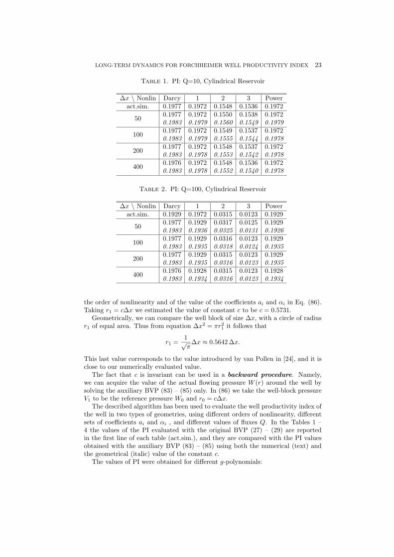
the order of nonlinearity and of the value of the coefficients ai and αi in Eq. (86).Taking r1 = c∆x we estimated the value of constant c to be c = 0.5731.

Geometrically, we can compare the well block of size ∆x, with a circle of radiusr1 of equal area. Thus from equation ∆x2 = πr21 it follows that

r1 =1√π∆x ≈ 0.5642∆x.

This last value corresponds to the value introduced by van Pollen in [24], and it isclose to our numerically evaluated value.

The fact that c is invariant can be used in a backward procedure. Namely,we can acquire the value of the actual flowing pressure W (r) around the well bysolving the auxiliary BVP (83) – (85) only. In (86) we take the well-block pressureV1 to be the reference pressure W0 and r0 = c∆x.

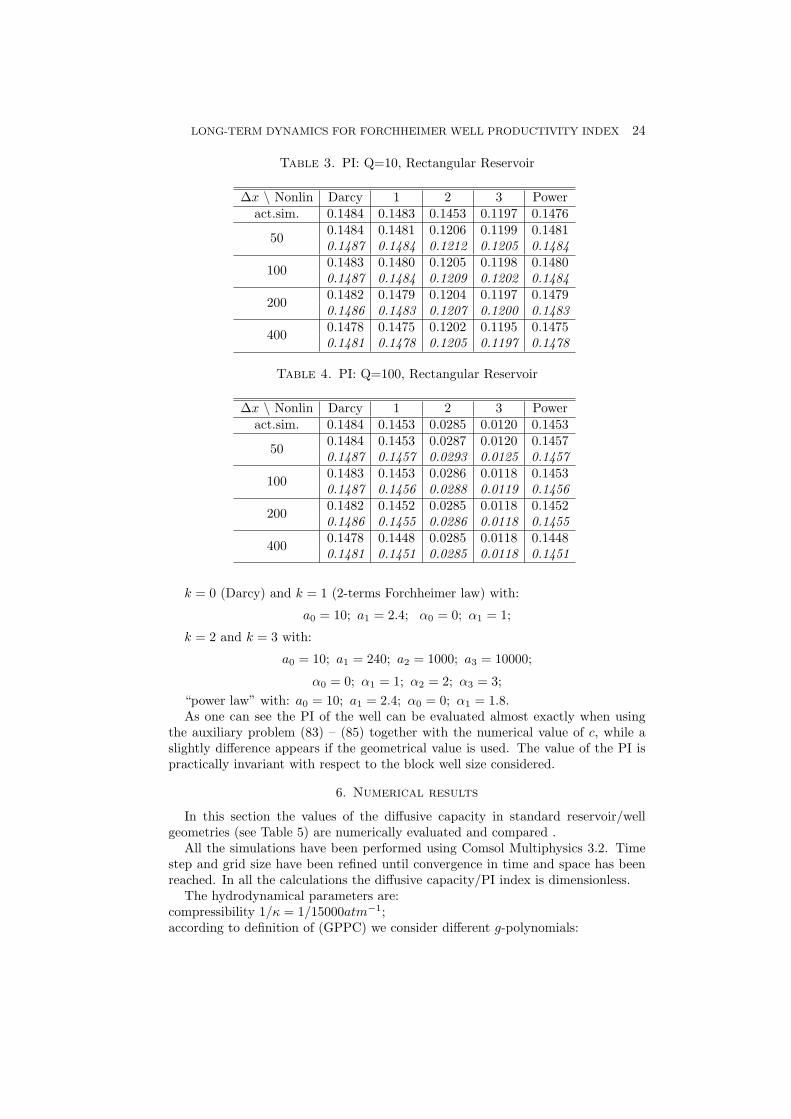
The described algorithm has been used to evaluate the well productivity index ofthe well in two types of geometries, using different orders of nonlinearity, differentsets of coefficients ai and αi , and different values of fluxes Q. In the Tables 1 –4 the values of the PI evaluated with the original BVP (27) – (29) are reportedin the first line of each table (act.sim.), and they are compared with the PI valuesobtained with the auxiliary BVP (83) – (85) using both the numerical (text) andthe geometrical (italic) value of the constant c.

The values of PI were obtained for different g-polynomials:


Table 3. PI: Q=10, Rectangular Reservoir


500.1484 0.1481 0.1206 0.1199 0.14810.1487 0.1484 0.1212 0.1205 0.1484

1000.1483 0.1480 0.1205 0.1198 0.14800.1487 0.1484 0.1209 0.1202 0.1484

2000.1482 0.1479 0.1204 0.1197 0.14790.1486 0.1483 0.1207 0.1200 0.1483

4000.1478 0.1475 0.1202 0.1195 0.14750.1481 0.1478 0.1205 0.1197 0.1478

Table 4. PI: Q=100, Rectangular Reservoir


500.1484 0.1453 0.0287 0.0120 0.14570.1487 0.1457 0.0293 0.0125 0.1457

1000.1483 0.1453 0.0286 0.0118 0.14530.1487 0.1456 0.0288 0.0119 0.1456

2000.1482 0.1452 0.0285 0.0118 0.14520.1486 0.1455 0.0286 0.0118 0.1455

4000.1478 0.1448 0.0285 0.0118 0.14480.1481 0.1451 0.0285 0.0118 0.1451

k = 0 (Darcy) and k = 1 (2-terms Forchheimer law) with:

a0 = 10; a1 = 2.4; α0 = 0; α1 = 1;

k = 2 and k = 3 with:

a0 = 10; a1 = 240; a2 = 1000; a3 = 10000;

α0 = 0; α1 = 1; α2 = 2; α3 = 3;

“power law” with: a0 = 10; a1 = 2.4; α0 = 0; α1 = 1.8.As one can see the PI of the well can be evaluated almost exactly when using

the auxiliary problem (83) – (85) together with the numerical value of c, while aslightly difference appears if the geometrical value is used. The value of the PI ispractically invariant with respect to the block well size considered.

6. Numerical results

In this section the values of the diffusive capacity in standard reservoir/wellgeometries (see Table 5) are numerically evaluated and compared .

All the simulations have been performed using Comsol Multiphysics 3.2. Timestep and grid size have been refined until convergence in time and space has beenreached. In all the calculations the diffusive capacity/PI index is dimensionless.

The hydrodynamical parameters are:compressibility 1/κ = 1/15000atm−1;according to definition of (GPPC) we consider different g-polynomials:


Table 5. Geometries

Shape Parameters

rw

re

circle

radius of reservoirre = 10000cm

reservoir thicknessH = 1000cmwell radiusrw = 30cm

2L

= 4

000

cmx

x 1L = 8000 cm

D=500

rectangle

Lx1 = 8000cmLx2 = 4000cmrw = 30cmH = 1000cmD = 500cm

L=

1/4

L

3/2

o60

L=10000 cm

triangle

L = 8000cmd = 2000cmrw = 30cmH = 1000cm

L x 2

x 1L

L wθ

fractures 00, 450, 900

(frac.-0; 45; 90)

Lx1 = 8000cmLx2 = 4000cmrw = 30cm

Lw = 3800cmH = 1000cmvarying angleθ = 00, 450, 900

θ

cylinderre = 10000cmH = 8000cmrw = 30cm

Lw = 8000cm

varying angleθ = 00, 150, 300,450, 600, 750

k = 0 (Darcy) and k = 1 (2-term Forchheimer law) with

a0 = 10; a1 = 2.4; α0 = 0; α1 = 1;


Table 6. Table of well Productivity Index, PSS regime - 2D case

flux circle triangle rectangle fract.-0 fract.-45 fract.-90Darcy 0.1977 0.1456 0.1484 0.9523 1.2092 1.4893

Q = 1 0.1976 0.1456 0.1483 0.9523 1.2092 1.4893k=1 Q = 10 0.1972 0.1453 0.1480 0.9521 1.2089 1.4889

Q = 100 0.1929 0.1426 0.1453 0.9502 1.2064 1.4853Q = 1 0.1975 0.1455 0.1482 0.9522 1.2091 1.4892

power Q = 10 0.1966 0.1449 0.1476 0.9515 1.2081 1.4879Q = 100 0.1910 0.1412 0.1439 0.9469 1.2022 1.4800Q = 1 0.1928 0.1426 0.1453 0.9502 1.2064 1.4853

k=2 Q = 10 0.1548 0.1182 0.1204 0.9312 1.1814 1.4506Q = 100 0.0315 0.0281 0.0285 0.7707 0.9770 1.1817Q = 1 0.1927 0.1425 0.1452 0.9502 1.2064 1.4853

k=3 Q = 10 0.1183 0.0956 0.0971 0.9311 1.1813 1.4503Q = 100 0.0005 0.0005 0.0005 0.7463 0.9367 1.1156

k = 2 and k = 3 with

a0 = 10; a1 = 240; a2 = 1000; a3 = 10000;

α0 = 0; α1 = 1; α2 = 2; α3 = 3;

“power law“: a0 = 10; a1 = 2.4; α0 = 0; α1 = 1.8;in 2D case Q/H = 1, 10, 100cm2/s;in 3D case Q = 8 ∗ 103, 8 ∗ 104, 8 ∗ 105cm3/s;

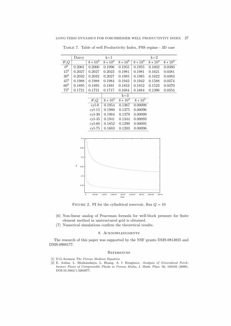
Tables 6 and 7 report the numerical values of the well Productivity Index for PSSregime for different non-linearities, different values of total flux Q and for differentshapes of the reservoirs for 2D and 3D geometries respectively. It can be seen thatthe higher is the order of nonlinearity of g-polynomial the smaller is the value ofPI.

On example of the cylindrical reservoir with a fully penetrated vertical well lo-cated at the center we present numerical study of the behavior of transient diffusivecapacity depending on the non-linearity of g-polynomial.

The time evolution of transient PI is reported in Fig.2. Here total flux is constantQ = 10. The curve above represents the values of PI in linear Darcy case, the curvebelow represents the PI for the 2-term Forchheimer law. As expected the linear PIis always distinctly greater than non-linear PI, and each of them stabilizes in timeto corresponding PSS PI values.

7. Conclusions

(1) Well Productivity Index can be modeled as a functional over a solution ofdegenerate parabolic equation.

(2) An accurate method for evaluation of the time invariant productivity indexhas been proposed.

(3) Convergence of transient Forchheimer PI to corresponding PSS value isproved for the wide class of boundary conditions and arbitrary initial data.

(4) Estimate for the difference between Forchheimer and Darcy PI’s in term ofparameters of Forchheimer polynomial and rate Q is obtained.

(5) Exact formula for the so called skin factor is derived.


Table 7. Table of well Productivity Index, PSS regime - 3D case

Darcy k=1 k=2θ\Q 8 ∗ 103 8 ∗ 104 8 ∗ 105 8 ∗ 103 8 ∗ 104 8 ∗ 10500 0.2001 0.2000 0.1996 0.1955 0.1955 0.1602 0.0380150 0.2027 0.2027 0.2023 0.1981 0.1981 0.1621 0.0381300 0.2032 0.2032 0.2027 0.1985 0.1985 0.1622 0.0383450 0.1988 0.1988 0.1984 0.1942 0.1942 0.1588 0.0374600 0.1895 0.1895 0.1891 0.1853 0.1852 0.1523 0.0370750 0.1721 0.1721 0.1717 0.1684 0.1684 0.1396 0.0354

k=3θ\Q 8 ∗ 103 8 ∗ 104 8 ∗ 105cyl-0 0.1954 0.1367 0.00098cyl-15 0.1980 0.1375 0.00096cyl-30 0.1984 0.1379 0.00099cyl-45 0.1941 0.1344 0.00093cyl-60 0.1852 0.1299 0.00095cyl-75 0.1683 0.1203 0.00096

0.15

0.2

0.25

0.3

0.35

0.4

0 5e+06 1e+07 1.5e+07 2e+07 2.5e+07 3e+07 3.5e+07 4e+07

PI

Time

Figure 2. PI for the cylindrical reservoir, flux Q = 10

(6) Non-linear analog of Peaceman formula for well-block pressure for finiteelement method in unstructured grid is obtained.

(7) Numerical simulations confirm the theoretical results.

8. Acknowledgments

The research of this paper was supported by the NSF grants DMS-0813825 andDMS-0908177.

References

[1] D.G.Aronson The Porous Medium Equation[2] E. Aulisa, L. Bloshanskaya, L. Hoang, A. I. Ibragimov, Analysis of Generalized Forch-

heimer Flows of Compressible Fluids in Porous Media, J. Math. Phys. 50, 103102 (2009),DOI:10.1063/1.3204977.


[3] E. Aulisa, A. I. Ibragimov, J. R. Walton, A new method for evaluation the productivity indexfor non-linear flow, SPE Journal, SPE Journal, Volume 14, Number 4, 693–706, (2009),DOI:10.2118/108984-PA.

[4] E. Aulisa, A. I. Ibragimov, P. P. Valko, J. R. Walton, Mathematical Frame-Work For Pro-ductivity Index of The Well for Fast Forchheimer (non-Darcy) Flow in Porous Media. Pro-ceedings of COMSOL Users Conference 2006, Boston (2006).

[5] E. Aulisa, A. Cakmak, A. Ibragimov, A. Solynin, Variational Principle and Steady State In-

variants for Non-Linear Hydrodynamic Interactions in Porous Media, Dynamics of Continu-ous, Discrete and Impulsive Systems, Series A Supplement, Advances in Dynamical Systems14 (S2) 148 (2007).

[6] E. Aulisa, A. Ibragimov, M. Toda, Geometric Framework for Modeling Nonlinear Flows in

Porous Media and Its Applications in Engineering, Nonlinear Analysis: Real World Appli-cations, in press (2009), DOI:10.1016/j.nonrwa.2009.03.028.

[7] E. Aulisa, A. I. Ibragimov, P. P. Valko, J. R. Walton, Mathematical Frame-Work ForProductivity Index of The Well for Fast Forchheimer (non-Darcy) Flow in Porous Me-

dia, Mathematical Models and Methods in Applied Sciences (M3AS), 8, 1241-1275, (2009),DOI:10.1142/S0218202509003772.

[8] M. T. Balhoff, A. Mikelic, M. F. Wheeler, Polynomial Filtration Laws for Low Reynolds

Number Flows Through Porous Media, Transport in Porous Media, in press (2009),DOI:10.1007/s11242-009-9388-z.

[9] J. Bear, Dynamics of Fluids in Porous Media, Dover Publications, Inc., New York, 1972.[10] T. A. Blasingame, L.E. Doublet, P.P. Valko, Development and application of the multiwell

Productivity Index (MPI), SPE Journal, 5(1) (2000), PP. 21-31.[11] L. P. Dake, Fundamental in reservoir engineering. Elsevier, Amsterdam, 1978.[12] J. Jr. Douglas, P. J. Paes-Leme, T. Giorgi, Tiziana Generalized Forchheimer flow in porous

media, Boundary value problems for partial differential equations and applications, 99–111,

RMA Res. Notes Appl. Math., 29, Masson, Paris, 1993.[13] L. C. Evans, Partial Differential Equations. American Mathematical Society, Providence,

1998.[14] E. Ewing, R. Lazarov, S. Lyons, D. Papavassiliou, Numerical well model for non Darcy flow,

Comp. Geosciences, 3, 3-4, (1999) 185–204.[15] P. Forchheimer, Wasserbewegung durch Boden Zeit, Ver. Deut. Ing. 45, (1901).[16] W. Helmy, R.A.Wattenbarger, New Shape Factors for Wells Produced at Constant Pressure,

Proceedings of SPE Gas Technology Symposium, SPE 39970, Calgary, Canada, 1998.

[17] L. Hoang, A. Ibragimov, Structural Stability of Generalized Forchheimer Equations for Com-pressible Fluids in Porous Media, 2010, submited for publication, preprinthttp://www.ima.umn.edu/preprints/jan2010/2294.pdf.

[18] A. I. Ibragimov, D. Khalmanova, P. P. Valko, J. R. Walton, On a mathematical model ofthe productivity index of a well from reservoir engineering, SIAM J. Appl. Math., 65 (2005),1952–1980.

[19] E. Landis, Second order equations of elliptic and parabolic type, Translations of Mathematical

Monographs, Vol. 171(1998), AMS, Providence, RI.[20] J.- L. Lions, Quelques mthodes de rsolution des problmes aux limites non linaires, Gauthier-

Villars, 1969[21] M. Muskat, The flow of homogeneous fluids through porous media. McGraw-Hill Book Com-

pany, Inc., New York and London, 1937.[22] L. E. Payne, B. Straughan, Convergence and Continuous Dependence for the Brinkman-

Forchheimer Equations. Studies in Applied Mathematics, 102 (1999), 419–439.[23] D. W. Peaceman, Interpretation of Well-Block Pressures in Numerical Reservoir Simulation.

SPE 6893 (1989), 183–192.[24] van Pollen H.K., Breitenbach, E.A. and Thurnau. D.H..Treatment of Individual Wells and

Grids in Reservoir Modeling, Soc. Pet. Eng. J. (Dec. 1968), 341–346. Trans., AIME, Vol.243.[25] R. Raghavan, Well Test Analysis. Prentice Hall, New York 1993.

[26] H.C. Slider, Worldwide Practical Petroelum Reservoir Engineering Methods., PennWell Pub-lishing Company, 1983.

[27] Schlumberger online dictionary URL:

http://www.glossary.oilfield.slb.com/Display.cfm?Term=productivity%20index%20(PI).


Department of Mathematics and Statistics, Texas Tech University, Box 41042, Lub-bock, TX 79409–1042, U. S. A.

E-mail address: [email protected]

E-mail address: [email protected] address: [email protected]

long-term dynamics for well productivity …bloshanl/research_files/abi11.pdf · long-term dynamics...

Documents