long-term multi-risk assessment: statistical treatment of ... · long-term multi-risk assessment:...

Natural Hazards manuscript No.(will be inserted by the editor)

Long-term multi-risk assessment: statistical treatmentof interaction among risks

Jacopo Selva

Received: date / Accepted: date

Abstract Multi-risk approaches have been recently proposed to assess and com-1

pare different risks in the same target area. The key points of multi-risk assess-2

ment are the development of homogeneous risk definitions and the treatment of3

risk interaction. The lack of treatment of interaction may lead to significant bi-4

ases and thus to erroneous risk hierarchization, which is one of primary output5

of risk assessments for decision makers. In this paper, a formal statistical model6

is developed to treat interaction between two different hazardous phenomena in7

long-term multi-risk assessments, accounting for possible effects of interaction at8

hazard, vulnerability and exposure levels. The applicability of the methodology9

is demonstrated through two illustrative examples, dealing with the influence of10

(i) volcanic ash in seismic risk and (ii) local earthquakes in tsunami risk. In these11

applications, the bias in single-risk estimation induced by the assumption of in-12

dependence among risks is explicitly assessed. An extensive application of this13

methodology at regional and sub-regional scale would allow to identify when and14

where a given interaction has significant effects in long-term risk assessments, and15

thus it should be considered in multi-risk analyses and risks hierarchization.16

Keywords multi-risk · multi-hazard17

1 Introduction18

In most of the areas in the world, more than one hazard may act in the same19

time frame, leading to different risks. Until recent years, risks were often assessed20

with different definitions/approaches/assumptions, making them substantially not21

comparable (e.g., [24]). Recently, different analyses and case studies have been22

proposed in order to make comparable assessments, with the goal of comparing and23

J. SelvaIstituto Nazionale di Geofisica e Vulcanologia, sezione di Bologna, Via Donato Creti 12 - 40128Bologna, ItalyTel.: +39-051-4151457Fax: +39-051-4151499E-mail: [email protected]

2 Jacopo Selva

ranking the different risks (e.g., [15,17,13]). Very recently, the analysis of cascade24

(or domino) effects highlighted the importance of the interaction among different25

risks, demonstrating that in multi-risk approaches the different risks should not26

only be compared, but also made interact [6,24,23].27

Classical risk assessments are based on the independence of risks, and thus28

may be substantially biased due to the fact that this assumption is not always29

and/or everywhere true. For example, the assessment of expected damages due30

to a given hazard is commonly made through vulnerability assessments based on31

fragility models of the target assets. The structural analyses usually adopted to32

develop fragility curves are based on the assumption of not perturbed structures,33

that is, only one specific hazard acts on the structure at the same time (e.g., [29]).34

In this case, it is evident that the possible simultaneous action of two hazards is35

not considered at all. Such interactions are of course in many case statistically ir-36

relevant. However, on one hand, many times the eventuality of two hazards acting37

at the same time is not unlikely at all, like for example when one hazard increases38

the probability of occurrence of a second hazard (e.g., earthquakes during vol-39

canic eruptions) or the two hazards may share a common source (e.g., seismic40

and tsunami hazards), or when the action of one hazard covers quite large time41

windows (e.g., snow on roofs of buildings). On the other hand, the consequence of42

simultaneous hazards may be so catastrophic that their impact on risk assessments43

may be significant, even in case of a rare simultaneous events.44

Focusing on one specific hazard, the mechanism leading to losses in case of45

single or simultaneous events is the same. For example, focusing on seismic risk,46

inter-story drift may be used as leading criterium for damages in case of ground47

shaking (e.g., [32]), both in presence or in absence of volcanic ash on roofs. There-48

fore, each specific mitigation action (e.g., retrofit, land-use plans, etc) decreases49

the total risk, that is, both single- and multi- risk components. Thus, a complete50

and coherent risk comparison is meaningful only when such interactive effects are51

accounted for. In other words, the bias of single-risk assessments (without inter-52

action) may lead to erroneous assessments of risks hierarchy and actions’ priority.53

A quantitative analysis of this possible bias in long-term risk assessments is54

still lacking. Indeed, the treatment of interaction among risks is still a quite open55

field, in which several case studies of cascade effects have been developed [22,42,56

24], while a complete formalization of the problem is not available. Recently, such57

interaction at hazard level (multi-hazard) have been treated by [23], where the for-58

mal distinction between single non-interacting hazard and complete multi-hazard59

assessment is proposed. However, the interaction of risks may act also at levels60

other than hazard, fact that deserves a specific treatment. Indeed, in several case61

studies, it has been shown how the contemporaneous action of different hazards62

may significantly either change the response of assets to the hazards (vulnerability63

interaction, e.g., [22,42]), or induce changes to the distribution of ’goods’, as for64

example when people moves from their original ’standard’ position (exposure in-65

teraction, e.g., [20,38]). Even restricting to natural hazards only, such interaction66

is conceivable in many realistic cases, such as for earthquakes striking areas in67

which are present volcanic ash, snow, or even floods (different fragility, as in appli-68

cation 1); tsunami striking shortly after an earthquake (different exposure, as in69

application 2); generic events striking pre-damaged (and not repaired) structures70

by, for example, earthquakes (different fragility and exposure). In other words,71

significant interaction is possible at both vulnerability and exposure level.72

Long-term multi-risk assessment: statistical treatment of interaction among risks 3

In this paper, a formal procedure is developed to account for interaction in risk73

assessments at all levels (hazard, vulnerability and exposure), in the case of two74

interacting hazardous phenomena. In this framework, the effect of interaction on75

single loss/risk assessment can be quantitatively evaluated, and the assumption76

of complete independence of risks verified. Two illustrative applications are then77

presented, demonstrating the practical applicability of the methodology in real78

case studies.79

2 Interaction in multi-risk assessment80

The risk curve due to a generic event E1 for a given asset in a given exposure time81

∆T represents the probability that a given loss value l is overcome in a target82

area and in the exposure time ∆T . By use of the total probability rule, it can be83

written84

Rc(E1)(l) =

∫d

∫x

E(l|d) · dF(d|x) · dH(x) (1)

where l is a loss measure in a specific metrics, d a given damage measure, x a given85

hazard intensity measure, and86

– H(x) represents the cumulative hazard assessment (survivor function), in terms87

of its intensity x88

– F(d|x) represents the fragility of the target asset, that is, the probability that89

the damage level d is overcome due to an intensity x [13]90

– E(l|d) is the probability that a given loss level l is reached or overcome, given91

the damage level d. Since E(l|d) accounts for the consequence of damage d with92

its specific metrics (economic loss, casualties, dead), hereinafter it is referred93

to as the ‘exposure’ term.94

The formulation in Eq. 1 represents a generalization for a generic ∆T of the Pacific95

Earthquake Engineering Research (PEER) formula [10,12], it may be used as a96

general formulation for any kind of natural risks [23], and formally it holds for97

small probabilities for the hazardous phenomenon [34]. Given the large number98

of symbols used throughout the paper, in Tab. 1 a complete list of symbols is99

reported.100

In case of non-systemic risk assessments (e.g., [7]), losses due to different assets101

in the target area can be assessed independently and then summed up over all the102

present assets (e.g., damages to buildings in seismic risk [40]). Commonly, damages103

d, for each single asset, are expressed through a discrete number of damage states104

di (e.g., [29]). In addition, also the hazard assessment is commonly approximated105

for discrete intervals of intensity xj (e.g., [4]). With these simplifications and using106

the notations in Tab. 1, Eq. 1 becomes107

Rc(E1)(l)≈∑i

{E(E1)(l|di) ·

[∑j

δF(E1)(di|xj) · δH(E1)(xj)

]}(2)

where the symbol δ, instead of d, is used, to highlight the discretization. The108

superscript (E1) indicates that all the quantities refer to the specific hazardous109

phenomenon E1 (e.g., ground shaking). The term into square brackets is often110

referred to as physical vulnerability (e.g., [14]), and it represents the probability111

4 Jacopo Selva

that a damage state di is observed for the asset in the exposure time. In its112

cumulative form reads113

PV (E1)(di) =∑j

F(E1)(di|xj) · δH(E1)(xj) (3)

A quite special case, but very common for most of natural hazards, occurs when114

the hazard term H(E1)(xj) is assumed Possonian, with annual rate λ(E1)≥xj

. In this115

case, also the physical vulnerability is Poissonian (from [9]), with annual rates116

λ(E1)≥di =

∑j

F(E1)(di|xj) · δλ(E1)≥xj

(4)

which is numerically equivalent to Eq. 3 for small λ(E1)xj [12]. This formulation al-117

lows to automatically account for the repeatability of the hazardous phenomenon118

(many earthquakes in the exposure time), problem that should be specifically ad-119

dressed in Eq. 3 in case of significant probability of multiple events in the exposure120

time [34].121

In many areas, two hazardous events (E1 and E2) can act on the same structure122

in the exposure time ∆T (e.g., ground shaking and snow). Interaction among the123

consequent risks occurs when E1 acts in a temporal windows in which E2, or124

its consequence, is still acting (e.g., ground shaking occurs when snow is present125

on roofs). If the effects of E2 may influence the expected losses due to E1, either126

through the exposure E(E1) and/or the vulnerability F(E1), their consequences are127

completely neglected whenever E1 risk is assessed through Eq. 2. In other words,128

to account for the interaction between E1 and E2 in losses/risk assessment of E1,129

it must be considered that for limited time windows (e.g., snow is present on roofs)130

the expected losses due to the event E1 are modified by E2, potentially influencing131

the overall long-term assessment. In other words, following the reported example,132

in assessing the probability of damages due to ground shaking in the exposure133

time ∆T , it must be considered that (i) the presence of snow on roofs alters the134

fragility F(E1) [22], and (ii) the snow is present only in limited time windows.135

To account for this interaction, the different contributions to damages due to136

E1 in presence or not of E2 should be factorized. The probability of E1 in ∆T in137

presence of the effects of E2 can be defined as138

H(E1,E2)(xj) = pr(≥ xj at time t in ∆T & t− tE2 < ∆Tp)= pr(≥ xj ;∆Tp|E2) · pr(E2,∆T ) =

= H(E1|E2)(xj ;∆Tp) · pr(E2,∆T )

(5)

which represents the probability that, during the exposure time∆T , E1 is preceded139

by E2 within a time window ∆Tp. In the second row, this probability is factorized140

in conditional probabilities, where H(E1|E2) represents the probability of x ≥ xj in141

a time window ∆Tp, given that E2 has occurred. Note that this does not necessary142

imply a cause-effect relationship between E1 and E2, but possibly just a temporal143

coincidence. The term pr(E2,∆T ) represents the probability of E2 in the exposure144

time ∆T . For sake of simplicity, just at this stage, the secondary event E2 is145

assumed Boolean (yes/no), but this restriction will be overcome in paragraph 2.2.146

The time window ∆Tp, herein referred to as persistence time window, represents147

for how long the effect of E2 will be active after the occurrence of the event E2,148


so potentially influencing E1 vulnerability or exposure terms. The length of ∆Tp149

strongly varies for different E2. To better understand the meaning of all terms150

in 5, we can follow the example reported above (E1 is ’ground shaking’, E2 is151

’snow on roofs’): pr(E2,∆T ) is the probability of significant snow in ∆T , ∆Tp is152

the time window in which snow melts, and H(E1,E2) represents the probability of153

significant ground shaking in presence of snow.154

Since the events x ≥ xj within ∆Tp after E2 represent a subset of the events155

x ≥ xj in ∆T , the hazard H(E1,E2) is only a part of the total E1 hazard H(E1);156

thus157

H(E1)(≥ xj) = H(E1,E2)(≥ xj) +H(E1,E2)(≥ xj) (6)

where H(E1,E2) is the same of Eq. 5, and H(E1,E2) represents the probability158

of x ≥ xj in ∆T not preceded by an event E2 in ∆Tp. Following the reported159

example, H(E1,E2) represents the probability of ground shaking in ∆T when snow160

is not present on roofs. Hereinafter, H(E1,E2) and H(E1,E2) will be referred to as161

co-active and isolated-hazard factors, respectively. Note that this factorization is162

similar to the one proposed by [23] for multi-hazard assessments. The fundamental163

difference is that this factorization specifies a temporal limit ∆Tp for interaction.164

Without this specification, none of the following developments would be possible.165

The probability of damages ≥ di due to any xj is evaluated by assessing the166

physical vulnerability through Eq. 3. However, the two complementary (to the167

total hazard) hazard factors now must be kept separated, that is:168

PV (E1)(≥ di) =∑j F

(E1,E2)(≥ di|xj) · δH(E1,E2)(xj)

+∑j F

(E1,E2)(≥ di|xj) · δH(E1,E2)(xj)(7)

where different symbols for the fragility terms are reported, to highlight that they169

should be evaluated in condition of occurrence and non-occurrence of E2, respec-170

tively. Following the reported example, F(E1,E2) represents the fragility to ground171

shaking assuming snow on roofs, while F(E1,E2) assumes no snow on roofs.These172

two fragilities, as discussed above, may significantly differ in these two different173

conditions.174

To complete the risk analysis, the consequences of damages should be consid-175

ered through the exposure term, as in Eq. 2. The expression for the PV (E1) can176

be substituted in Eqs. 3 and 2, obtaining177

Rc(E1)(≥ l) = Rc(E1,E2)(≥ l) +Rc(E1,E2)(≥ l) (8)

where178 {Rc(E1,E2)(≥ l) =

∑i E

(E2)(l|di)∑j δF

(E1,E2)(di|xj) · δH(E1,E2)(xj)

Rc(E1,E2)(≥ l) =∑i E

(E2)(l|di)∑j δF

(E1,E2)(di|xj) · δH(E1,E2)(xj)(9)

and, as for fragilities above, different symbols for the exposure terms are reported,179

in condition of occurrence or non-occurrence of E2.180

In Eqs. 8 and 9, the contributions to the total risk of the co-active and the181

isolated-risk factors result completely separated. With this formulation, the effects182

of interaction on damaging are accounted for whenever risk is assessed. Since only183

in this case a complete risk assessment in a multi-risk perspective is made, Rc(E1)184

will be referred to as multi-risk for E1.185

6 Jacopo Selva

The co-active risk factor Rc(E1,E2) represents the risk posed by the event E1186

in the time lapses ∆Tp, in which it is active the hazard E2. The effects of E2 in187

both fragility and exposure are accounted for in this term. Considering Eq. 5, the188

co-active risk factor reads189 {Rc(E1,E2)(≥ l) =

∑i E

(E2)(l|di) · δPV (E1|E2)(di) · pr(E2;∆T )

PV (E1|E2)(di) =∑j δF

(E1,E2)(di|xj) · δH(E1|E2)(xj)(10)

where the physical vulnerability δPV (E1|E2) is highlighted. This vulnerability is190

exactly as a canonical physical vulnerability, but it is conditioned to the occur-191

rence of the event E2 and it is referred to a time window ∆Tp. Following the192

reported example, this risk term refers to losses occurring when ground shaking193

strike structures covered by snow.194

The isolated risk factor Rc(E1,E2) represents the residual risk posed by E1,195

when this is not influenced by the occurrence of E2. To better understand its196

meaning, it can be rewritten in light of Eq. 6, so that197

Rc(E1,E2)(≥ l) =∑i E

(E2)(l|di)∑j δF

(E1,E2)(di|xj) · δH(E1,E2)(xj) =

= Rc(E1,s)(≥ l)−Rc(E1,v)(≥ l)(11)

where the two terms identified have a clear physical meaning. Indeed, the first198

term199 {Rc(E1,s)(≥ l) =

∑i E

(E2)(l|di) · δPV (E1,s)(di)

δPV (E1,s)(di) =∑j δF

(E1,E2)(di|xj) · δH(E1)(xj)(12)

represents the risk evaluated considering the isolated fragility δF(E1,E2) and ex-200

posure E(E2) factors, and the total hazard δH(E1)(≥ xj). This is what it is usu-201

ally done in the literature, whenever the hazard is assessed from undifferentiated202

catalogs [23]. For this reason, Rc(E1,s) will be referred to as single-risk for E1.203

Following the reported example, this risk term considers fragility and exposure204

evaluated assuming no snow on roofs, while hazard is assessed independently from205

the fact that snow is present on roofs.206

The second term in Eq. 11 reads207 {Rc(E1,v)(≥ l) =

∑i E

(E2)(l|di) · δPV (E1|E2,v)(di) · pr(E2;∆T )

δPV (E1|E2,v)(di) =∑j δF

(E1,E2)(di|xj) · δH(E1,E2)(xj)(13)

and it represents the risk that would have been forecast in case of occurrence208

of E2, if no changes to fragility and exposure were expected. Since the physical209

vulnerability term δPV (E1|E2,v) has the same meaning of δPV (E1|E2) in Eq. 10, it210

is used the same symbol with the addition of v, to highlight that the fragility term211

here is the isolated one, instead of the coactive one. Rc(E1,v) will be referred to as212

virtual risk factor, and it is fundamental to compensate the coactive-risk factor in213

Eq. 10. Indeed, if both fragility and exposure are not affected by the occurrence214

of E2 (fragility and exposure to ground shaking are equal, with or without snow),215

Rc(E1,E2) equals Rc(E1,v), for all l, and thus, from Eq. 8,216

Rc(E1)(≥ l) = Rc(E1,s)(≥ l) (14)


meaning that the multi-risk assessment Rc(E1), in this case, is exactly equal to217

the single-risk assessment Rc(E1,s), for all l.218

In practice, the multi-risk analysis can be performed through Eqs. 8 and 9.219

The coactive-risk factor Rc(E1,E2) is assessed though Eq. 10. The assessment of220

the isolated risk factor Rc(E1,E2) is based either on a direct assessment through221

Eq. 11, first row, or through the evaluation of the two further risk factors, that is,222

the single risk factor Rc(E1,s) (Eq. 12) and the virtual risk factor Rc(E1,v) (Eq.223

13).224

All physical vulnerability terms share the same functional form, that is:225

PV (∗) =∑j

F(∗)(≥ di|xj) · δH(∗)(xj) (15)

which is identical to the classical assessment, as reported in Eq. 3. In case of226

Poissonian hazards, they can also be assessed through 4, as commonly reported227

in the literature (e.g., [14]). However, it is worth noting that PV (E1,s) (single-risk228

factor, Eq. 12) is referred to the hazard of E1 in the exposure time ∆T . On the229

contrary, both PV (E1|E2) (co-active risk factor, Eq. 10) and PV (E1|E2,v) (virtual-230

risk factor, Eq. 13) are referred to time windows ∆Tp just after the occurrence of231

E2 in ∆T . During these periods, all terms (including the hazard term H(E1,E2))232

may be largely influenced [23].233

2.1 Single-risk assessment and its bias234

In the literature, sometimes only one of the two hazard factors in Eq. 6 is assessed,235

but more commonly they are assessed jointly like, for example, when hazard is236

assessed from undifferentiated catalogs [23]. On the contrary, just one fragility237

term is usually assessed (the isolated one), that is, the one in absence of external238

influences (e.g., [29]). The same is valid for the exposure term, for which either239

the variability due to external factors (day/night, summer/winter) or a averaged240

value is assumed, but in any case not considering the effects of E2. Since, in case241

of occurrence of E2, one or more of these terms may be potentially significantly242

influenced, single-risk assessment may result significantly biased.243

To evaluate the effective strength of the interaction among risks, in the fol-244

lowings single and multi-risk assessments are compared, as assessed through Eqs.245

8 and 12, respectively. In the single-risk formulation, the assessment is based on246

the isolated fragility F(E1,E2) and exposure E(E2) terms, and the total hazard247

H(E1)(≥ xj). This is the case in most of applications, even though sometimes248

H(E1,E2) is assessed instead. In these cases, the single-risk assessment is equal to249

the isolated risk factor Rc(E1,E2) in Eq. 8.250

In order to allow a simpler comparison among the same risk in different areas,251

as well as, different risks in the same area, a single risk index is often considered,252

instead of using the whole risk curve (e.g., [24]). As risk index, the average (mean)253

of losses in the target area in the exposure time is considered, which reads:254

R(∗) =

∫l

l · dRc(∗)(≥ l) =

∫l

∫d

∫x

l · dE(l|d) · dF(d|x) · dH(x) =

≈∑i

l(∗)ave(di) · δPV (∗)(≥ di)(16)

8 Jacopo Selva

where l(∗)ave(di) is the average loss caused by the damage state di for the generic255

(∗) risk factor (e.g., [5]). The risk index R(∗) is often expressed for ∆T = 1 year256

and, in the case of earthquakes, referred to as Average Annual Earthquake Losses257

(AEL in [28]). The average in Eq. 16 applies to both the single-risk assessment,258

and to all the factors of the multi-risk assessment, so that259

R(E1,s) =∑i

l(E2)ave (di) · δPV (E1,s)(≥ di)

R(E1) ≡ R(E1,E2) +R(E1,s) −R(E1,v) =

=∑i

l(E2)ave (di) · δPV (E1|E2)(≥ di) · pr(E2;∆T )

+∑i

l(E2)ave (di) · δPV (E1,s)(≥ di)

−∑i

l(E2)ave (di) · δPV (E1|E2)(≥ di) · pr(E2;∆T )

(17)

The bias that a single-risk assessment introduces, since it does not account for260

the effects of E2, reads:261

δR(E1) = R(E1) −R(E1,s) = R(E1,E2) −R(E1,v) =

=∑ij

[l(E1,E2)ave (di)δF(E1,E2)(di|xj)− l(E2)

ave (di)δF(E1,E2)(di|xj)]δH(E1,E2)(xj) =

=∑j

[L(E1,E2)(xj)− L(E1,E2)(xj)

]δH(E1,E2)(xj)

(18)and, normalized by the single-risk:262

δR(E1)/R(E1,s) =

∑j

[L(E1,E2)(xj)− L(E1,E2)(xj)

]δH(E1,E2)(xj)∑

j L(E1,E2)(xj)δH(E1)(xj)(19)

This means that the bias depends, for each level of intensity xj , on two factors:263

(i) how strong the interaction at damaging level is (the term in brackets), and (ii)264

how probable it is the occurrence of the event E1, within the persistence time265

window ∆Tp, just after E2 in ∆T .266

In many cases, the bias of single-risk assessments will be negligible. In particu-267

lar, this is certainly true whenever (i) pr(E2) ≈ 0 (approximately no E2 hazard),268

that is, δH(E1,E2) ≈ 0, or (ii) the damaging term is not influenced by E2, that is,269

L(E1,E2)(xj) = L(E1,E2)(xj), for all xj .270

In other cases, a more specific analysis of both terms is necessary. A quite271

common situation is when E1 and E2 are two independent and rare events, that272

is273

δH(E1,E2) = pr(E1;∆Tp) · pr(E2;∆T ) (20)

due to their independence, and274

δH(E1,E2) = pr(E1;∆Tp) · pr(E2;∆T )� pr(E1;∆T ) = δH(E1) (21)

due to the fact that pr(E2;∆T ) � 1 and pr(E1;∆Tp) < pr(E1;∆T ), for all275

intensity levels x. This means, in practice, that the possibility of concomitant276

events E1 and E2 is quite rare. However, this can be sufficient to neglect the bias277

only assuming that this difference in probability is sufficient to compensate the278


increase in vulnerability due to E2. This is valid only if L(E1,E2) is smaller, but279

approximately of the same order of magnitude, of L(E1,E2), at all intensity levels280

x. In general, this can be the case, but a careful assessment of both isolated and281

coactive-vulnerability factors should be preferable.282

Whenever the events E1 and E2 effectively interact, that is, the occurrence283

of E2 increases the probability of E1, it is surely necessary a careful evalua-284

tion of both terms. Indeed, δH(E1|E2) may be close to 1 and then δH(E1,E2) ∼285

pr(E2;∆T ), that is, all the hazard terms have the same order of magnitude. In286

this case, R(E1) and R(E1,s) may actually significantly differ.287

2.2 From Boolean to discrete intensity values288

In most of cases, the secondary event E2 cannot be considered as Boolean, since289

different intensities for E2 may lead to different levels of interaction with the E1290

risk terms.291

The influence of the different levels of intensity of E2 must be considered in292

both the co-active (all terms) and the virtual-risk (hazard term) factors. Starting293

from the co-active risk factor R(E1,E2) in Eq. 10, it is noted that the event E2 can294

lead to different levels of intensity yk, with probability pr(yk|E2). By definition,295

the yk, for all k and given the occurrence of E2, represent a complete and mutually296

exclusive set of events (∑k pr(yk|E2) = 1), and thus:297

Rc(E1,E2)(l) ≡∑i E

(E2)(l|di)∑j δF

(E1,E2)(di|xj)δH(E1,E2)(xj) ≡≡ pr(≥ l|E2)pr(E2;∆T ) ==[∑

k pr(≥ l|E2)pr(yk|E2)]pr(E2;∆T ) =

=∑i,k[E(E2,yk)(l|di)

∑j δF

(E1,yk)(di|xj , yk)δH(E1|yk)(xj , yk)]δH(E2)(yk) =

=∑i,k E

(E2,yk)(l|di)δPV (E1|yk)(di|yk)δH(E2)(yk)

(22)where298

– each yk represents a specific interval of values for the intensity of E2, and the299

index k covers all possible values for the intensity, so that∑k pr(yk|E2) = 1300

– in the second row, all probability terms are highlighted using the symbol pr(e),301

which generically indicates the probability of the event e302

– for each of the original terms (first row), symbols are modified to highlight303

their potential dependence on the value yk. Hazard, fragility and exposure304

may all theoretically depend on yk. In practical applications, exposure is often305

not dependent on yk and can exit from the sum in k.306

– the term δH(E1|yk)(xj) represents the (discrete) non-cumulative hazard curve307

for the primary event E1 in the persistence time window ∆Tp after an event308

E2 with intensity yk in ∆T . This conditional hazard term, combined to the309

fragility, allows the assessment of the conditional physical vulnerability δPV (E1|yk)(di|yk),310

as identified in the last row. This physical vulnerability is equivalent to the one311

in Eq. 3, in its cumulative version, and it can be assessed as the ordinary one,312

but it is conditioned to the occurrence of E2 with intensity yk (one separate313

assessment for each k), and relative to the time window ∆Tp.314

– the term pr(yk|E2)pr(E2) is identified as the (discrete) non-cumulative hazard315

curve for the secondary event E2, in the exposure time ∆T , i.e., δH(E2)(yk).316

10 Jacopo Selva

The formulation in Eq. 22 allows accounting for the effects on hazard, fragility317

and exposure of the different intensities of E2. Of course, all these additional terms318

need specific assessments, strongly increasing the effort necessary for a complete319

multi-risk assessment. However, on one side, not necessarily both vulnerability and320

exposure depend on yk, on the other side, the width of E2 intensity intervals (the321

number of yk) can be rather large (i.e., few ks), depending on the sensitivity on y322

of the E1 risk terms.323

The same development is necessary for the virtual-risk factor, in Eq. 13. The324

result is exactly the same, but in this case neither fragility nor exposure terms do325

depend on E2, and consequently on yk, that is326

Rc(E1,v)(l) =∑i,k[E(E2)(l|di)

∑j δF

(E1,E2)(di|xj)δH(E1|yk)(xj , yk)]δH(E2)(yk) =

=∑i,k E

(E2)(l|di)δPV (E1|yk,v)(di|yk)δH(E2)(yk)

(23)where in each physical vulnerability term (one for each k), there is a dependence327

on yk only at the hazard level, if any. In any case, as for PV (E1|yk)(di|yk) in Eq.328

22, each one of these terms is equivalent to the one in Eq. 3. Thus, as above,329

it can be assessed as the ordinary physical vulnerability, but it is conditioned to330

the occurrence of E2 with intensity yk (one separate assessment for each k), and331

relative to the time window ∆Tp.332

Equations 22 and 23 contain the hazard terms in both xj and yk. The to-333

tal (discrete) non-cumulative hazard curve for the primary event E1, in case of334

occurrence of E2, can be derived by marginalizing with respect to yk, that is:335

δH(E1,E2)(xj) =∑k

δH(E1|yk)(xj)δH(E2)(yk) (24)

Note that, if there is not a specific dependence between the intensity of primary336

and secondary events, as in most of real cases, this expression again collapses to337

the formulation in Eq. 5, since δH(E1|yk) does not depend on yk and can exit from338

the sum, and thus the sum simply becomes the probability of the event E2 in ∆T .339

3 Applications340

3.1 Case study 1: fragility dependence in ground-motion/ash-fall interaction341

This application focuses in assessing the long-term seismic risk (E1 ≡ ground342

shaking) related to economic loss, in presence (E2) and in absence (E2) of previous343

volcanic eruptions with significant ash fall (loading > 3 kPa) [42]. In particular, it344

is discussed here the effect of a possible increase of the vulnerability to earthquakes345

when buildings’ roofs are loaded by significant ash. This increase is discussed in346

[42] and it is reported here as illustrative example of interaction at the fragility347

level.348

This illustrative analysis is indicatively located in the area of Naples (Italy).349

This area is subject to seismic hazard due to both tectonic earthquakes located350

the Apennines chain, and to seismic events located in the nearby volcanic areas351

(e.g., [8]). In addition to this, this area is subject to significant volcanic hazard due352

to the three active volcanoes in the Neapolitan area, Mt. Vesuvius, Campi Flegrei353


and Ischia (e.g., [3]). For this application, an exposure time ∆T of 50 years is354

selected, in agreement with the official seismic hazard for Italy [18]. For simplicity,355

it is considered as target just one specific building, of a specific class.356

The seismic fragility curves adopted are the ones in [42] for a class Bs building,357

that is, good masonry with iron beam floor. Such fragility curves change for various358

levels of ash load on the roof. The fragility in presence of significant ash loading359

(F(E1,yk)) can be deduced from the one in absence of loading (F(E1,E2)), with the360

relationship proposed in Tab. 8 of [42] with loading variable from 3 to 20 kPa, at361

intervals of 1 kPa. No significant changes to fragilities are expected for y < 3 kPa.362

The seismic intensity adopted for seismic hazard (xj) is macro-seismic intensity363

EMS92. Such fragility curves consider 5 damage states, ranging from minor to364

complete damages.365

The exposure E(l|di) is assumed not dependent on the presence or absence of366

ash loading. For simplicity, the uncertainty on the losses due to each di is not367

considered (e.g., [39,5]), in which case the distribution E(l|di) can be modelled as368

a step function θ centered on an average value lave(di). The average loss lave is369

set as RC · CDFi, that is, the ’replacement cost’ RC of the structure multiplied370

by the ’cost damage factor’ CDFk, which represents the fraction of RC to repair371

the k-th damage state [39], that is372 {l(E2,yk)ave (di) = l

(E2)ave (di) = RC · CDFi

E(E2,yk)(l|di) = E(E2)(l|di) = θ(RC · CDFi − l)(25)

In order to provide numerical results, RC is set to 10 million Euro (MEuro), and373

CDFi is set as in Tab. 2. These values are reliable and not critical, since in common374

for both single and multi-risk assessments.375

3.1.1 Single-risk assessment376

The single-risk assessment is performed implementing Eq. 12. As total seismic377

hazard, the annual rates for the city of Naples (LAT 40.8322, LON 14.2832, ID:378

33201) provided by the official Italian hazard map [18,41] are taken, where PGA379

values are transformed to macroseismic EMS92 intensity values as in [27]. For380

simplicity, epistemic uncertainties are neglected, and only the best guess curve is381

considered. This hazard assessment formally includes also volcanic sources and it382

is produced starting from an undifferentiated seismic catalogue. This hazard is in383

the Poissonian form, and reads384

H(E1)(xj) = 1− exp{−λ(E1)xj·∆T} (26)

where the annual rates λ(E1)xj are available online [21]. The obtained seismic hazard385

curve for ∆T = 50 years is reported in Figure 1.386

Since H(E1) is Poissonian, the physical vulnerability PV (S1;s)(≥ di) can be387

assessed through Eq. 4, that is388 {PV (S1;s)(≥ di) = 1− exp{−λ(E1,s)

≥di ∆T}λ(E1,s)≥di =

∑j F

(E1,E2)(≥ di|xj)× δλ(E1)xj

(27)

12 Jacopo Selva

where the fragility models for Bs building are available in [42]. The single-risk389

curve is then evaluated by substituting in Eq. 12, that is390

Rc(E1,s)≥l =

∑i

θ(RC · CDFi − l) · δPV (S1;s)(≥ di) (28)

and it is reported in Figure 2 (black line).391

3.1.2 Multi-risk assessment392

The multi-risk assessment is performed through Eqs. 8 and 9, as modified in Eqs.393

22 and 23 for non Boolean E2.394

The co-active risk factor is evaluated through Eq. 10. To assess the volcanic395

hazard H(E2)(yk), ash loadings ≥ 3 kPa, up to 10 kPa, with intervals of 1 kPa, are396

considered. Under the assumption of independence of time intervals, this hazard397

can be set as398

H(E2)(≥ yk) = 1−[1− pr(ER) · pr(≥ yk|ER)

]12·∆Tk=1,2,...,10 (29)

where pr(ER) is the probability of eruption per month, whose a reliable order of399

magnitude for the volcanoes in the Napolitan area is 1 ·10−3 per month [25,26,35],400

and pr(≥ yk|ER) represents the probability to have ash loading ≥ yk given the401

occurrence of an eruption. To set this probability, a target point 4 km eastward402

of eruptive vent is selected and the hazard is modelled as in COMBO1 analysis403

in [36] (in which the Bayesian Event Tree method is set for the Campi Flegrei404

caldera). The COMBO1 analysis considers 4 possible eruption’s sizes for 1 specific405

eruptive vent, typical configuration of most of central volcanoes, and it is used406

here to derive the entire hazard curve for all the yk values. For simplicity, also in407

this case, epistemic uncertainties are neglected and only the best guess curve is408

considered. The obtained hazard curve is reported in Figure 3. The distance of 4 km409

is reasonable in the Napolitan area, since it represents approximately the distance410

between Naples (central area) and the most likely vent position for the Campi411

Flegrei caldera [37]. Of course, the results will strongly depend on this distance412

and here only one representative value is selected. Indeed, the quantification in all413

the urbanized areas around the volcano is important, but it is beyond the goals of414

this illustrative application.415

The seismic hazard, conditioned to the occurrence of E2, is assumed to not416

depend on yk, meaning that it is assumed to be equal for all eruptions. To set417

reliable values for HE1|E2(xj), it is noted that (i) the persistence time is quite418

long and, for this application, ∆Tp is set to 3 months [8], (ii) it is quite unlikely419

concomitant earthquakes and volcanic eruptions, except for the case of earthquakes420

occurring during the eruptive dynamics. As first approximation, the syn-eruptive421

seismicity is assumed Poissonian, that is422

H(E1|E2)(xj) = 1− exp{−λ(E1|E2)xj

·∆Tp} (30)

The annual rates are calculated from the 1982-84 seismicity at Campi Flegrei [11].423

Macro-seismic intensities are estimated from Ms and attenuated for distances of 4424

km as in [42]. The resulting non cumulated monthly rates, dλ(E1|E2)xj are reported in425

Figure 4, with maximum expected intensities at site equal to 7 (epicentral intensity426


8). Note that, a rather spread seismicity is expectable, so that the attenuation427

selected might underestimate peak intensities at the target site. On the other hand,428

it is noted that the 1982-84 did not lead to eruptions. On one side, higher intensities429

are expected during crises leading to eruptions (e.g., the maximum macroseismic430

intensity registered during the last eruption, Monte Nuovo 1582 AD, is 10 [19]).431

On the other side, most of those seismic events are expected before the actual432

eruption. However, the eruption sizes that contribute more to the hazard are quite433

large (classes 3 and 4 in [31]), for which a complex eruptive dynamics is expected,434

with several eruptive phases [30]. For comparison with the total hazard reported435

above (H(E1), as used in the single-risk assessment), the combined seismic hazard436

curve, as computed applying Eq. 24, is reported in Figure 1 (grey dots).437

The physical vulnerability of the co-active risk factor is then assessed through438

Eq. 4, so that439 {PV (E1|yk)(≥ di|yk) = 1− exp{−λ(E1|yk)

≥di ·∆Tp}λ(E1|yk)≥di =

∑j F

(E1,yk)(≥ di|xj , yk) · δλ(E1|E2)xj

(31)

in which fragility functions are set as in Table 8 of [42], and the hazard is set as in440

Eq. 30. The co-active risk factor can be evaluated by substituting in Eqs. 22 and441

10, that is442

Rc(E1,E2)(≥ l) =∑i

θ(RC · CDFi − l)∑k

δPV (E1|yk)(di|yk)δH(E2)(yk) (32)

where the volcanic hazard term is assessed as in Eq. 29. The obtained co-active443

risk factor is reported in Figure 2 (dashed line).444

The isolated risk factor is assessed through Eq. 11, from the single-risk and445

virtual-risk factors. The single-risk term is exactly the one assessed above, for the446

single-risk assessment, as reported in Figure 2 (black line). The virtual-risk factor447

can be assessed directly from Eq. 13, since there is not dependence of the E1448

hazard on yk. The physical vulnerability, as above, is assessed through Eq. 4, that449

is450 {PV (E1|E2,v)(≥ di) = 1− exp{−λ(E1|E2,v)

≥di ·∆Tp}λ(E1|E2,v)≥di =

∑j F

(E1,E2)(≥ di|xj) · δλ(E1|E2)xj

(33)

where the fragilities are exactly the same adopted above for the single-risk assess-451

ment (Eq. 27), while the annual rates are the ones adopted to assess the co-active452

risk factor (Eq. 31). The virtual-risk factor is then evaluated by substituting in453

Eq. 13 (or, equivalently, Eq. 23), that is454

Rc(E1,v)(≥ l) =∑i

θ(RC · CDFi − l)δPV (E1|E2,v)(di)H(E2)(≥ y1) (34)

and it is reported in Figure 2 (dotted line).455

The final multi-risk curve, as obtained through Eqs. 8 and 11, is reported in456

Figure 2 (grey line).457

14 Jacopo Selva

3.1.3 Single vs Multi-risk assessments458

The bias between single (black) and multi-risk (grey) curves is evident in Figure 2.459

A more quantitative evaluation of this bias is given by average losses (risk index).460

By substituting in Eq. 17, the single-risk assessment reads:461

R(E1,s) = RC ·∑i

CDFi · δPV (S1;s)(≥ di) = 1.2003 MEuro (35)

and for the multi-risk assessment:462 R(E1) = R(E1,E2) +R(E1,s) −R(E1,v) =

= RC ·∑i,k CDFi · δPV

(E1|yk)(di|yk)δH(E2)(yk)

+RC ·∑i CDFi · δPV

(S1;s)(≥ di)−RC ·

∑i,k CDFi · δPV

(E1|yk,v)(di|yk)δH(E2)(yk) =

= 1.3389 MEuro

(36)

that is, the bias of single-risk assessment results:463 {δR(E1) = 0.13859 MEuro

δR(E1)/R(E1,s) = 0.115 ≈ 10%(37)

These results are based on very first-order, but reasonable values, and they464

show that the single-risk assessment underestimates the actual risk by about 10465

percent. It is important to note that this results strongly depend on the selected466

position, since the long-term volcanic hazard decays quite quickly with distance467

(e.g., [36]). Therefore, this bias could strongly vary also at urban scale, affecting in468

a non-uniform manner the total multi-risk assessment. This bias, together with the469

intrinsic epistemic uncertainties associated to any risk assessment [1], could have470

large effects on the resulting risk hierarchization presented to decision makers, at471

least in specific areas.472

3.2 Case study 2: exposure dependence in tsunami/earthquake interaction473

This application focuses in assessing the tsunami risk (E1 ≡ tsunami) related to474

human life losses, in presence and in absence of a previous seismic event (E2 is a475

significant earthquake) that can influence the exposure in coastal areas. In partic-476

ular, it is investigated here the effect on tsunami risk of changes in the exposure477

to tsunamis due to local strong earthquakes striking the target area. Indeed, such478

local earthquakes may significantly modify the exposure to tsunamis, either in-479

creasing it (e.g., concentration in seaside areas of people escaping from damaged480

buildings), or decreasing it (spontaneous evacuation of seaside areas of adequately481

informed population). This effect is here reported as illustrative example of inter-482

action at the exposure level. For significant earthquakes, events strong enough to483

generate significant damages in the target area are considered, so that such dam-484

ages could induce changes to the tsunami exposure. It is set, as risk metrics, the485

number of deaths and, for simplicity, only direct effects of tsunami are considered.486

An exposure time of 1 year (∆T = 1 yr) is considered.487

With these choices, only one damage state contribute to the loss assessment488

(d1 ≡ d means ’death’). The fragility (mortality) of persons exposed to tsunami489


waves is independent from the occurrence/non-occurrence of significant earth-490

quakes in the area. In this application, the formulation in [33] is assumed, where491

the rates of deaths (and injuries) as functions of water depth are assessed by us-492

ing information from both the survey and prior events for the 17 July 2006 Java493

tsunami. This fragility function reads:494

F(E1,E2)(d = 1|xj) = F(E1,E2)(d = 1|xj) = F(d = 1|xj) ≈0.4

10xj (38)

where xj is expressed in meter. In this formulation, differences (e.g., age, sex, etc.)495

among the people exposed to the tsunami waves are not considered.496

As regards the exposure, each person counts as one in the risk assessment.497

The total risk should consider the total number of people exposed to tsunami498

in the target area. While an explicit formulation for the total risk curve is more499

complicated, under the assumption of identical and independent individuals and500

identical capability in movements at all times (day/night, summer/winter), the501

risk index can be written as502

R(∗) =

∫d

∫x

< N (∗) >t ·dF(d|x) · dH(x) (39)

where < N (∗) >t is the average number (in time) of exposed people to tsunamis of503

intensity x, and it plays the role of l(∗)ave in Eq. 16. For simplicity, this application504

is then limited to the assessment of risk indexes, in order to quantify the bias505

between single- and multi-risk assessments.506

In general, in case of non occurrence of E2, the number of exposed people507

strongly varies through time, in particular for day/night as well as summer/winter508

changes, and its average reads509

l(E2)ave =

1

∆T

∫ ∆T

0

N(t)dt ≡ Nave (40)

In case of occurrence of E2, the number of exposed persons may drastically510

vary. Indeed, it may be extremely high if the population is not correctly informed511

about tsunamis, since many people can move to the seaside in order to escape512

from falling buildings (e.g., Lisbon 1755, Messina 1908). If, on the opposite, the513

population has been adequately prepared to the risk of tsunamis, the exposure to514

tsunamis may be very low (provided that they have sufficient time to evacuate),515

since the informed population runs toward less exposed areas (e.g., Padang 2009).516

In either case, in first approximation, it does not depend on time, so that517

l(E2)ave = NEQ (41)

which can be, for limited time windows, very different from Nave.518

To assess the single-risk index, the total hazard curve for a given location is con-519

sidered. In Fig. 5, for example, it is reported the tsunami hazard curve δHE1(xj)520

for a representative location offshore Seaside, Oregon, as obtained by [16]. Note521

that this hazard curve is not obtained for inundation, and also it is relative to a522

completely different environment with respect to fragilities. Thus, the risk assess-523

ment obtained by combining this hazard curve with the fragility reported above524

16 Jacopo Selva

is only really indicative, with the solely goal of illustrating a complete analysis.525

Applying Eq. 17, first row, single-risk indexes can be assessed as526

R(E1,s) =∑i

Nave · δF(d = 1|xj) · δH(E1)(xj) = Nave × 1.4 · 10−3 (42)

where δH(E1)(xj) is the non-cumulative hazard curve relative to the target coast-527

line area.528

To assess the multi-risk index, the hazard factor H(E1,E2)(≥ xj) must be529

defined, that is, the probability in ∆T that a significant seismic event E2 occurs,530

followed within ∆Tp by a tsunami with intensity ≥ xj . The persistence time ∆Tp531

can be approximately set to few hours, that is the time after which people start532

moving back to cities, and/or emergency actions start taking place. The probability533

to have a tsunami within few hours after an earthquake that causes large damages534

in the target coastline is surely very low, unless the tsunami is caused by the535

earthquake itself or by close in time aftershocks. Thus, the term H(E1,E2)(xj)536

essentially refers to the tsunami caused by earthquakes close enough to the target537

area to cause significant damages to structures. This allows a more quantitative538

definition of significant earthquakes, since such events must be strong enough539

to generate significant tsunami ( e.g., M > 7), and close enough to generate540

significant damages due to seismic waves (e.g., at distances < 100 km). Note that541

all the other possible tsunamis, due to either distant earthquakes or non-seismic542

sources, for which no significant seismic damages are experienced at the target543

site, will contribute through the isolated hazard term H(E1,E2).544

In Figure 5, the contribution to the hazard curve of near seismic sources (green545

line), and the one of the other (only seismic, in this case) sources (red lines)546

are individuated [16], allowing the identification of δH(E1,E2)(xj). This allows an547

explicit assessment of the multi-risk factors, since the co-active risk factor reads548

R(E1,E2) = NEQ∑j δF(d = 1|xj) · δH(E1,E2)(xj) =

= NEQ × 1.6 · 10−4 (43)

where δH(E1,E2)(xj) is the hazard related to the near seismic sources. The virtual-549

risk factor reads550

R(E1,v) = Nave∑j δF(d = 1|xj) · δH(E1,E2)(xj) =

= Nave × 1.6 · 10−4 (44)

that is, obviously, equal to co-active risk factor, a part for the number of exposed551

persons.552

The multi-risk index can finally be computed:553

R(E1) = R(E1,E2) +R(E1,s) −R(E1,v) == [0.16 ·NEQ + 1.24 ·Nave] · 10−3 (45)

and the bias between single and multi-risk assessed:554 {δR(E1) = 0.16 · (NEQ −Nave) · 10−3

δR(E1)/R(E1,s) = 0.11 · (NEQ

Nave− 1)

(46)

Note that, in this illustrative application, a significant bias (> 0.05, that is,555

5%) is obtained already for an increase of 50% of the exposure in presence of E2556


(NEQ = 1.5 · Nave), which is a rather small increase in case of significant local557

earthquakes. Note also that δR also quantifies the long-term benefit (decrease of558

risk) in case of correct education of people and/or management plan about the559

possibility of tsunamis just after a large local earthquake, in which case NEQ ≈560

0. In this case, indeed, the earthquake works as an efficient precursor for local561

tsunamis, reducing the long-term tsunami risk by ≈ 10%.562

4 Final Remarks563

The presented method allows a full assessment of one specific long-term risk, con-564

sidering the interaction that its terms may have with other hazards and/or external565

events. Beside considering interaction at the hazard level (e.g., [23]), the method566

focuses to the possibility that one secondary hazard triggers changes to the vul-567

nerability and exposure terms relative to the primary hazard (e.g., [42]). To do568

that, the method (i) makes use of interacting (sometimes called time-dependent)569

vulnerability and exposure terms, in which the effect on the target assets of com-570

bined hazards is accounted for, and (ii) it introduces the concept of persistence571

time window for the hazard that triggers the interaction. Combining such terms572

with the hazard assessments, the presented method allows an explicit quantifica-573

tion (eqs. 8 and followings) of the long-term risk associated to the primary hazard574

in a multi-risk perspective, that is, considering risk interactions at all levels. This575

quantification finally allows an explicit estimate (eqs. 18 and 19) of the bias that576

it is induced by neglecting risk interactions (as in single-risk analyses), and thus577

an explicit assessment of the statistical significance in long-term risk assessments578

of any conceivable interaction among two risks.579

In assessing risk, the method makes use of fully aggregated hazard assessments.580

This characteristic makes it applicable in systematic analyses of the strength of581

interactions in extended target areas, since it does not imply large computational582

efforts. This is of primary importance, since only such systematic analyses (i) al-583

low identifying if and where a specific interaction is significant and thus when it is584

important to consider strictly multi-hazard/risk procedures, and (ii) may help im-585

plementing effective multi-risk mitigation actions, focusing to specific interactions586

and selected areas.587

This method is limited to applications with only two interacting risks. In sev-588

eral case studies, however, more than two hazards may potentially interact in the589

same area. In theory, the developed method could be recursively extended to more590

than two hazards, but this further development would lead to an explosion in the591

number of the terms necessary to the analysis (e.g., all terms could eventually592

depend on three or more intensity measures). On the other side, the presented593

method may be applied to each couple of hazards, and it may be used to filter594

out interactions that lead to statistically non significant effects in long-term risk595

assessments. In alternative, other methods considering combinations of single sce-596

narios (cascade events) may be applied (e.g., [2]). However, the large number of597

scenarios to be considered in long-term risk assessments may limit their effective598

applicability.599

18 Jacopo Selva

Acknowledgements600

The work described in this paper has been carried out in the framework of the601

project Quantificazione del Multi-Rischio con approccio Bayesiano: un caso stu-602

dio per i rischi naturali della citta di Napoli (2010-2013), funded by the Ital-603

ian Ministry of Education, Universities and Research (Ministero dell’Istruzione,604

dell’Universita e della Ricerca) [1].605


Fig. 1 Complete (black) and co-active (grey) Probabilistic Seismic Hazard Assessment in thearea of Naples (Italy), with an exposure time ∆T = 50 years. The co-active hazard factorconsiders only seismic event occurring in presence of significant ash loading (> 3 kPa) onroofs, within a persistence time window ∆Tp = 3 months.

Fig. 2 Seismic risk curves in the area of Naples (Italy), with an exposure time ∆T = 50 years.Single (black) and multi-risk (grey) assessments are reported, together with multi-risk factors,i.e., the co-active (dashed grey line) and the virtual (dotted grey line) ones.

Fig. 3 Probabilistic Volcanic Hazard Assessment for ash fall in the area of Naples (Italy),with an exposure time ∆T = 50 years. This hazard curve is assessed assuming a target area4 km eastward of a possible eruptive vent, with 4 possible eruption sizes typical of the CampiFlegrei caldera, Italy (see text for more details).

Fig. 4 Annual rates of macroseismic intensity at site (attenuated at 4 km) during the 1982-1984 unrest episode in Campi Flegrei, Italy. See text for more details.

Fig. 5 Probabilistic Tsunami Hazard Assessment offshore Seaside, Oregon, as obtained by[16]. With different colours, the distinct contributions to the hazard of near (green) and other(red) sources are highlighted.

20 Jacopo Selva

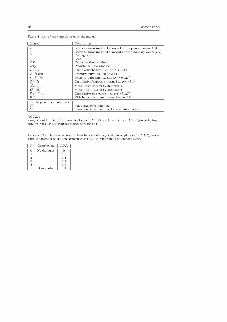
Table 1 List of the symbols used in the paper.

Symbol Description

x Intensity measure for the hazard of the primary event (E1)y Intensity measure for the hazard of the secondary event (E2)d Damage statel Loss∆T Exposure time window∆Tp Persistence time window

H(∗)(x) Cumulative hazard, i.e., pr(≥ x;∆T )

F(∗)(d|x) Fragility curve, i.e., pr(≥ d|x)

PV (∗)(d) Physical vulnerability, i.e., pr(≥ d;∆T )

E(∗)(l) Cumulative ’exposure’ term, i.e., pr(≥ l|d)

l(∗)ave(d) Mean losses caused by damages d

L(∗)(x) Mean losses caused by intensity x

Rc(∗)(≥ l) Cumulative risk curve, i.e., pr(≥ l;∆T )

R(∗) Risk index, i.e., herein mean loss in ∆T

for the generic cumulative FdF non-cumulative functionδF non-cumulative function, for discrete intervals

NOTES:∗ may stand for: ‘E1, E2’ (co-active factor); ‘E1, E2’ (isolated factor); ‘E1, s’ (single factor,only for risk); ‘E1, v’ (virtual factor, only for risk)

Table 2 Cost damage factors (CDF s) for each damage state in Application 1. CDFk repre-sents the fraction of the replacement cost (RC) to repair the k-th damage state.

di Description CDFi

0 No damages 01 0.12 0.23 0.64 0.85 Complete 1.0


References606

1. ByMuR project: Quantificazione del Multi-Rischio con approccio Bayesiano: un caso studio607

per i rischi naturali della citta di Napoli (Bayesian Multi-Risk assessment: a case study608

for natural risks in the city of Naples) (2010-2013). URL http://bymur.bo.ingv.it609

2. MATRIX - New Multi-Hazard and Multi-Risk Assessment Methods for Europe (2010-610

2013). URL http://matrix.gpi.kit.edu611

3. Alberico, I., Petrosino, P., Lirer, L.: Volcanic hazard and risk assessment in a multi-source612

volcanic area: the example of Napoli city. Natural Hazards - Earth System Science (11),613

1057–1970 (2011). DOI 10.5194/nhess-11-1057-2011614

4. Bazzurro, P., Cornell, C.: Disaggregation of seismic hazard. Bulletin of the Seismological615

Society of America 89(2), 501–520 (1999)616

5. Bommer, J., Spence, R., Erdik, M., Tabuchi, S., Aydinoglu, N., Booth, E.,617

del Re, D., Peterken, O.: Development of an earthquake loss model for Turk-618

ish catastrophe insurance. Journal of Seismology 6, 431–446 (2002). URL619

http://dx.doi.org/10.1023/A:1020095711419. 10.1023/A:1020095711419620

6. Bovolo, A., Abele, S., Bathurst, J., Caballero, D., Ciglan, M., Eftichidi, G., Simo, B.:621

A distributed framework for multi-risk assessment of natural hazards used to model the622

effects of forest fire on hydrology and sediment yield. Computers and Geosciences 35,623

924–945 (2009). DOI 10.1016/j.cageo.2007.10.010624

7. Cavalieri, F., Franchin, P., Gehl, P., Khazai, B.: Quantitative assessment of social625

losses based on physical damage and interaction with infrastructural systems. Earth-626

quake Engineering and Structural Dynamics (2012). DOI 10.1002/eqe.2220. URL627

http://dx.doi.org/10.1002/eqe.2220628

8. Convertito, V., Zollo, A.: Assessment of pre-crisis and syn-crisis seismic hazard at Campi629

Flegrei and Mt. Vesuvius volcanoes, Campania, southern Italy. Bulletin of Volcanology630

73, 767–783 (2011). DOI 10.1007/s00445-011-0455-2631

9. Cornell, C.: Engineering seismic risk analysis. Bulletin of the Seismological Society of632

America 58, 1583–1606 (1968)633

10. Cornell, C., Krawinkle, H.: Progress and challanges in seismic per-634

formance assessment. PEER Center News 3(2) (2000). URL635

http://peer.berkeley.edu/news/2000spring/index.html636

11. De Natale, G., Zollo, A.: Statistical analysis and clustering features of the Phlegraean637

Fields earthquake sequence (May 1983 - May 1984). Bulletin of the Seismological Society638

of America 76(3), 801–814 (1986)639

12. Der Kiureghian, A.: Non-ergodicity and PEER’s framework formula. Earthquake Engi-640

neering and Structural Dynamics 34, 1643–1652 (2005). DOI 10.1002/eqe.504641

13. Douglas, J.: Physical vulnerability modelling in natural hazard risk assessment. Natural642

Hazards - Earth System Science 7, 283–288 (2007)643

14. Elefante, L., Jalayer, F., Iervolino, I., Manfredi, G.: Disaggregation-based response weight-644

ing scheme for seismic risk assessment of structures. Soil Dynamics and Earthquake En-645

gineering 30, 1513–1527 (2010)646

15. FEMA: Multi hazard identification and risk assessment:a cornerstone of the national mit-647

igation strategy. Tech. rep., FEMA (1997)648

16. Gonzalez, F., Geist, E., Jaffe, B., Kanoglu, U., Mofjeld, H., Synolakis, C., Titov, V., Arcas,649

D., Bellomo, D., Carlton, D., Horning, T., Johnson, J., Newman, J., Parsons, T., Peters, R.,650

Peterson, C., Priest, G., Venturato, A., Weber, J., Wong, F., Yalciner, A.: Probabilistic651

tsunami hazard assessment at Seaside, Oregon, for near- and far-field seismic sources.652

Journal of Geophysical Research 114(C11023) (2009). DOI 10.1029/2008JC005132653

17. Grunthal, G., Thieken, A., Schwarz, J., Radtke, K., Smolka, A., Merz, B.: Comparative654

Risk Assessments for the City of Cologne – Storms, Floods, Earthquakes. Natural Hazards655

38(1-2), 21–44 (2006). DOI 10.1007/s11069-005-8598-0656

18. Gruppo di Lavoro: Redazione della mappa di pericolosita’ sismica prevista dall’Ordinanza657

PCM 3274 del 20 marzo 2003. Rapporto Conclusivo per il Dipartimento della Protezione658

Civile. Tech. rep., Istituto Nazionale di Geofisica e Vulcanologia, Milano-Roma (2004)659

19. Guidoboni, E., Ciucciarelli, C.: The Campi Flegrei caldera: historical revision and new data660

on seismic crises, bradyseisms, the Monte Nuovo eruption and ensuing earthquakes (twelfth661

century 1582 AD). Bulletin of Volcanology 73, 655–677 (2011). DOI 10.1007/s00445-010-662

0430-3663

22 Jacopo Selva

20. Guidoboni, E., Mariotti, D.: Il terremoto e il maremoto del 1908: effetti e parametri sismici.664

In: G. Bertolaso, E. Boschi, E. Guidoboni, G. Valensise (eds.) Il terremoto e il maremoto665

del 28 dicembre 1908: analisi sismologica, impatto, prospettive, p. 814pp. SGA edizioni666

(2008)667

21. INGV-DPC: Interactive Seismic Hazard Maps (2004). URL http://esse1-gis.mi.ingv.it668

22. Lee, K., Rosowsky, D.: Fragility analysis of woodframe buildings considering combined669

snow and earthquake loading. Structural Safety 28(3), 289–303 (2006)670

23. Marzocchi, W., Garcia-Aristizabal, A., Gasparini, P., Mastellone, M., Di Ruocco, A.: Basic671

principles of multi-risk assessment: a case study in Italy. Natural Hazards pp. 1–23 (2012).672

URL http://dx.doi.org/10.1007/s11069-012-0092-x. 10.1007/s11069-012-0092-x673

24. Marzocchi, W., Mastellone, M.L., Di Ruocco, A., Novelli, P., Romeo, E., Gasparini, P.:674

Principles of multi-risk assessment 2009. Principles of multi-risk assessment: interactions675

amongst natural and man-induced risks, Project Report - FP6 NARAS project (contract676

No. 511264). Tech. Rep. EUR23615, European Commision - Directorate-General Research677

– Environment (2009)678

25. Marzocchi, W., Sandri, L., Gasparini, P., Newhall, C., Boschi, E.: Quantifying probabilities679

of volcanic events: the example of volcanic hazard at Mt. Vesuvius. Journal of Geophysical680

Research 109(B11201) (2004). DOI 10.1029/2004JB003155681

26. Marzocchi, W., Sandri, L., Selva, J.: BET EF: a probabilistic tool for long- and short-term682

eruption forecasting. Bulletin of Volcanology 70, 623 632 (2008)683

27. Masi, A.: Seismic Vulnerability Assessment of Gravity Load Designed R/C Frames. Bul-684

letin of Earthquake Engineering 1, 371–395 (2003)685

28. NIBS: HAZUS99 Estimated Annualized Earthquake Losses for the United States. Tech.686

Rep. 366, Federal Emergency Management Agency, Washington, D.C. (2000)687

29. NIBS: HAZUS, Technical manuals, vol. Earthquake loss estimation methodology, federal688

emergency management agency edn. Washington, D.C. (2004)689

30. Orsi, G., Civetta, L., Del Gaudio, C., de Vita, S., di Vito, M.A., Isaia, R., Petrazzuoli,690

S., Ricciardi, G., Ricco, C.: Short-term ground deformations and seismicity in the nested691

Campi Flegrei caldera (Italy): an example of active block-resurgence in a densely populated692

area. Journal of Volcanology and Geothermal Research 91(2-4), 415–451 (1999)693

31. Orsi, G., Di Vito, M.A., Selva, J., Marzocchi, W.: Long-term forecast of eruption style and694

size at Campi Flegrei caldera (Italy). Earth and Planetary Science Letters 287, 265–276695

(2009)696

32. Pinto, P.E. (ed.): Probabilistic Methods for Seismic Assessment of Existing Structures,697

vol. LESSLOSS Report No. 2007/06. IUSS Press, Pavia, Italy (2007)698

33. Reese, S., Cousins, W., Power, W., Palmer, N., Tejakusuma, I., Nugrahadi, S.: Tsunami699

vulnerability of buildings and people in South Java - field observations after the July 2006700

Java tsunami. Natural Hazards - Earth System Science 7(5), 573–589 (2007)701

34. Ryden, J., Rychlik, I.: Probability and Risk Analysis, An Introduction for Engineers,702

springer edn. Springer Berlin / Heidelberg, Berlin NY (2006)703

35. Sandri, L., Guidoboni, E., Marzocchi, W., Selva, J.: Bayesian event tree for eruption704

forecasting (BET EF) at Vesuvius, Italy: a retrospective forward application to the 1631705

eruption. Bulletin of Volcanology 71(7), 729–745 (2009)706

36. Selva, J., Costa, A., Marzocchi, W., Sandri, L.: BET VH: Exploring the influence of natural707

uncertainties on long-term hazard from tephra fallout at Campi Flegrei (Italy). Bulletin708

of Volcanology 72(6), 717–733 (2010). DOI 10.1007/s00445-010-0358-7709

37. Selva, J., Orsi, G., Di Vito, M., Marzocchi, W., Sandri, L.: Probability hazard map for710

future vent opening at the Campi Flegrei caldera, Italy. Bulletin of Volcanology 74,711

497–510 (2012). DOI 10.1007/s00445-011-0528-2. 10.1007/s00445-011-0528-2712

38. Spahn, H., Hoppe, M., Vidiarina, H., Usdianto, B.: Experience from three years of lo-713

cal capacity development for tsunami early warning in Indonesia: challenges, lessons and714

the way ahead. Natural Hazards - Earth System Science 10, 1411–1429 (2010). DOI715

10.5194/nhess-10-1411-2010716

39. Stergiou, E., Kiremidjian, A.: Treatment of Uncertainties in Seismic Risk Analysis of717

Transportation Systems. Tech. Rep. 154, John A. Blume Earthquake Engineering Center,718

Civil Engineering Department, Stanford University, Stanford, CA (2006)719

40. Strasser, F., Bommer, J., Sesetyan, K., Erdik, M., Cagnan, Z., Irizarry, J., Goula, X.,720

Lucatoni, A., Sabetta, F., Bal, I., Crowley, H., Lindholm, C.: A Comparative Study of721

European Earthquake Loss Estimation Tools for a Scenario in Istanbul . Journal of Earth-722

quake Engineering 12(S2), 246–256 (2008). DOI 10.1080/13632460802014188723


41. Stucchi, M., Meletti, C., Montaldo, V., Crowley, H., Calvi, G.M., Boschi, E.: Seismic724

Hazard Assessment (2003-2009) for the Italian Building Code. Bulletin of the Seismological725

Society of America 101, 1885–1911 (2011)726

42. Zuccaro, G., Cacace, F., Spence, R., Baxter, P.: Impact of explosive eruption scenarios at727

Vesuvius. Journal of Volcanology and Geothermal Research 178, 416–453 (2008)728

long-term multi-risk assessment: statistical treatment of ... · long-term multi-risk assessment:...

Documents