long-term power system capacity expansion planning
TRANSCRIPT
Graduate Theses and Dissertations Iowa State University Capstones, Theses andDissertations
2011
Long-term power system capacity expansionplanning considering reliability and economiccriteriaYang GuIowa State University
Follow this and additional works at: https://lib.dr.iastate.edu/etd
Part of the Electrical and Computer Engineering Commons
This Dissertation is brought to you for free and open access by the Iowa State University Capstones, Theses and Dissertations at Iowa State UniversityDigital Repository. It has been accepted for inclusion in Graduate Theses and Dissertations by an authorized administrator of Iowa State UniversityDigital Repository. For more information, please contact [email protected].
Recommended CitationGu, Yang, "Long-term power system capacity expansion planning considering reliability and economic criteria" (2011). GraduateTheses and Dissertations. 10163.https://lib.dr.iastate.edu/etd/10163

Long-term power system capacity expansion planning considering reliability and economic criteria
by
Yang Gu
A dissertation submitted to the graduate faculty
in partial fulfillment of the requirements for the degree of
DOCTOR OF PHILOSOPHY
Major: Electrical Engineering
Program of Study Committee:
James D. McCalley, Major Professor Dionysios Aliprantis
Lizhi Wang Sarah Ryan Arka Ghosh
Iowa State University
Ames, Iowa
2011
Copyright © Yang Gu, 2011. All rights reserved

ii
Table of Contents
NOMENCLATURE .............................................................................................................. vii
LIST OF FIGURES ................................................................................................................ x
LIST OF TABLES ............................................................................................................... xiii
ACKNOWLEDGEMENTS ................................................................................................ xiv
CHAPTER 1 INTRODUCTION ........................................................................................... 1
CHAPTER 2 LITERATURE REVIEW ............................................................................... 6
2.1 SYSTEM CAPACITY EXPANSION PLANNING ALGORITHMS ................................................ 6
2.1.1 Generation Expansion Planning Algorithms ............................................................ 6
2.1.2 Transmission Expansion Planning Algorithms ........................................................ 9
2.2 SYSTEM CAPACITY EXPANSION PLANNING TOOLS ......................................................... 14
2.2.1 Introduction ............................................................................................................ 14
2.2.2 Production Cost Simulation Tools .......................................................................... 17
2.2.3 Resource Planning Tools ........................................................................................ 19
2.2.4 Reliability Assessment Tools ................................................................................. 20
2.2.5 National Planning Tools ......................................................................................... 22
CHAPTER 3 MODELING THE INTEGRATED ENERGY SYSTEM ......................... 25

iii
3.1 GENERALIZED NETWORK FLOW MODEL ........................................................................ 27
3.2 COMBINING DC POWER FLOW MODEL WITH GNF MODEL ............................................ 30
3.2.1 System Formulation ................................................................................................ 30
3.2.2 Nodal Prices ............................................................................................................ 31
3.3 NUMERICAL EXAMPLE ................................................................................................... 33
CHAPTER 4 RELIABILITY-BASED AND MARKET-BASED PLANNING .............. 44
4.1 RELIABILITY -BASED TRANSMISSION EXPANSION PLANNING ......................................... 47
4.1.1 Overall Formulation ............................................................................................... 47
4.1.2 Master Problem....................................................................................................... 48
4.1.3 Slave Problem ......................................................................................................... 49
4.1.4 Iteration Procedures ................................................................................................ 51
4.2 MARKET-BASED TRANSMISSION EXPANSION PLANNING ............................................... 52
4.2.1 Overall Problem ...................................................................................................... 52
4.2.2 Market Structure and Operation ............................................................................. 53
4.2.3 Master Problem....................................................................................................... 57
4.2.4 Slave Problem ......................................................................................................... 58
4.2.5 Iteration Procedures ................................................................................................ 60
4.3 NUMERICAL EXAMPLE ................................................................................................... 61
4.3.1 5-bus System........................................................................................................... 61
4.3.2 A 30-bus System ..................................................................................................... 65
iv
3.4.3 Scalability of The Market-based Planning Algorithm ............................................ 67
4.4 TRANSMISSION PLANNING CONSIDERING BOTH RELIABILITY AND ECONOMIC
CRITERIA .............................................................................................................................. 70
CHAPTER 5 MODELING UNCERTAINTIES ................................................................ 74
5.1 MONTE CARLO SIMULATION METHOD ........................................................................... 76
5.2 BENDERS DECOMPOSITION ITERATION PROCEDURES ..................................................... 79
5.3 ROBUSTNESS TESTING AND MULTIPLE FUTURES ............................................................ 82
5.4 NUMERICAL EXAMPLE ................................................................................................... 86
CHAPTER 6 TRANSMISSION PLANNING CONSIDERING LARGE-SCALE
INTEGRATION OF RENEWABLE ENERGY ................................................................ 89
6.1 INTRODUCTION ............................................................................................................... 89
6.2 WIND FORMULATION ..................................................................................................... 92
6.3 GENERATION EXPANSION PLANNING MODEL ................................................................. 93
6.3.1. Unit Commitment Problem Formulation ............................................................... 97
6.3.2. Economic Dispatch Problem Formulation .......................................................... 101
6.3.3. GEP Master Problem Formulation ...................................................................... 103
6.4 TRANSMISSION EXPANSION PLANNING MODEL ............................................................ 104
6.5 COORDINATING GEP AND TEP .................................................................................... 106
6.6 NUMERICAL EXAMPLE ................................................................................................. 107

v
CHAPTER 7 EVALUATING ENERGY STORAGE SYSTEM AS AN
ALTERNATIVE TO TRANSMISSION EXPANSIONS ................................................ 115
7.1 INTRODUCTION ............................................................................................................. 115
7.2 STORAGE MODEL ......................................................................................................... 117
7.3 CASE STUDY ................................................................................................................. 122
7.4 COMPARING THE ECONOMIC PERFORMANCE OF CAES AND TRANSMISSION LINE
ADDITIONS ......................................................................................................................... 131
CHAPTER 8 THE MARKET-BASED TRANSMISSION PLANNING TOOL .......... 133
8.1 INTRODUCTION ............................................................................................................. 133
8.2 INPUT DATA ................................................................................................................. 136
8.3 PREPROCESSOR ............................................................................................................. 138
8.3 MPS FILE GENERATION ................................................................................................ 139
8.4 OPTIMIZATION MODEL .................................................................................................. 141
8.4.1 Benders Decomposition and Monte Carlo Simulation ......................................... 141
8.4.2 System Long-term Performance Evaluation ......................................................... 144
CHAPTER 9 CONCLUSIONS .......................................................................................... 146
9.1 CONTRIBUTIONS ........................................................................................................... 146
9.2 FURTHER RESEARCH DIRECTIONS ................................................................................ 147
APPENDIX: DETAILS OF THE TEST SYSTEMS ....................................................... 152

vi
BIBLIOGRAPHY ............................................................................................................... 154

vii
NOMENCLATURE
A. Sets
T Set of time periods
M Set of arcs in the existing electric transmission network
Mf Set of arcs in the fuel transportation network
Mt Set of arcs that represent electric transmission system
Mn’ Arcs that represent potential lines
Mg Set of arcs that represent power generation processes for generators (excluding
wind farms)
Md Set of arcs that represent LSEs’ bidding curves
N Set of nodes
Nf Set of nodes in the fuel transportation network
Ng Set of generators (excluding wind farms)
Nt Set of transmission buses
Nw Set of wind farms
Ns Set of compressed air energy storage systems
Lij Set of linearization segments of the energy bidding from node i to node j
Sij Set of linearization segments of the spinning reserve bidding from node i to
node j

viii
NSij Set of linearization segments of the non-spinning reserve bidding from node i to
node j
Bi Set of nodes adjacent to node i
Gi Set of generator nodes connected to node i
B. Variables
eij(l,t) Energy flow segment l from node i to node j during period t
enij(l,t) Energy flowing segment l from node i to node j through potential line during
period t
fij(s,t) Spinning reserve bidding segment s from node i to node j during period t
gij(ns,t) Non-spinning reserve bidding segment ns from node i to node j during period t
Uij Unit commitment decision variable for generator ij
r i(t) Load curtailment at node i during time t
C. Parameters
Ceij(l,t) Per-unit cost of the energy flow segment l from node i to node j during period t
Csij(s,t) Per-unit cost of the spinning reserve bidding segment s from node i to node j
during period t
Cnij(ns,t) Per-unit cost of the energy flowing from node i to node j during period t
( , )e l tij Upper bound on the energy flowing from node i to node j, also expressed as
eij.max

ix
( , )e l tij Lower bound on the energy flowing from node i to node j, also expressed as
eij.min
ηij Efficiency parameter associated with the arc connecting node i to node j
ηii Efficiency parameter associated with the arc connecting CAES i from one time
step to the next
lol Load curtailment penalty factor
bij Susceptance of the arc between node i and node j, also expressed as Bij
t The tth time period
δw(t) System wind penetration level at time t
σwij Capacity factor for wind farm ij
woij(t) Nominal 1-MW wind power time series ij at time t
wcij The steps of wind power capacity expansion
Davg Average system power demand level
dj(t) Supply (if positive) or negative of the demand (if negative) at node j, during
time t
ruij Generator ij ’s up-ramp rate limit
rdij Generator ij ’s down-ramp rate limit
uij Unit commitment decision for generator ij
λi Locational marginal price at node i
a Load time in generation investments

x
LIST OF FIGURES
Fig. 2.1. Generation Expansion Planning Procedure. ............................................................... 7
Fig. 2.2. Transmission expansion planning procedure ........................................................... 10
Fig. 2.3. Classification of system capacity expansion planning tools .................................... 15
Fig. 2.4. A simplified diagram of system model..................................................................... 16
Fig. 2.5. A simplified diagram of modular packages .............................................................. 16
Fig. 2.6. A simplified diagram of integrated models .............................................................. 17
Fig. 3.1. A typical network flow diagram. .............................................................................. 28
Fig. 3.2. Representing a generator’s marginal cost curve ....................................................... 29
Fig. 3.3. The interactions between fuel transportation system and electric transmission
system ..................................................................................................................................... 30
Fig. 3.4. Five-node system with fuel suppliers. ...................................................................... 34
Fig. 3.5. Fuel transportation and storage system. ................................................................... 35
Fig. 3.6. Oil and natural gas prices ......................................................................................... 37
Fig. 3.7. Oil Storage level ....................................................................................................... 37
Fig. 3.8. Generation levels ...................................................................................................... 38
Fig. 3.9. Locational marginal prices ....................................................................................... 38
Fig. 3.10. Branch flows (with DC power flow) ...................................................................... 39
Fig. 3.11. Branch flow (no DC power flow) ........................................................................... 40
xi
Fig. 4.1. An example two-bus system ..................................................................................... 44
Fig. 4.2. Iterations between master and slave problems in the reliability-based planning ..... 52
Fig. 4.3. Generator marginal cost curve .................................................................................. 55
Fig. 4.4. Supply- and Demand-side bidding curves ................................................................ 56
Fig. 4.5. Iterations between master and slave problems in the market-based planning .......... 61
Fig. 4.6. Five-bus system with four fuel suppliers .................................................................. 61
Fig. 4.7. The thirty-bus system (six regions with seven interregional interconnections) ....... 66
Fig. 4.8. Transmission planning considering both economic benefits and reliability
requirement ............................................................................................................................. 71
Fig. 5.1. The flow chart of Benders decomposition iteration procedures ............................... 82
Fig. 6.1. Wind generation expansion planning model ............................................................ 95
Fig. 6.2. Transmission expansion planning model ............................................................... 105
Fig. 6.3. Coordinate the two planning processes .................................................................. 107
Fig. 6.4. IEEE 24-bus reliability test system ........................................................................ 108
Fig. 6.5. GEP results from the original system ..................................................................... 111
Fig. 6.6. GEP results from the fifth iteration ........................................................................ 112
Fig. 7.1. Fields of application of the different storage techniques according to energy
stored and power output ........................................................................................................ 116
Fig. 7.2. Storage system model ............................................................................................. 119
Fig. 7.3. IEEE 24-bus reliability test system ........................................................................ 122

xii
Fig. 7.4. CAES average charge/discharge pattern and LMPs at bus 21 under scenario 1 .... 125
Fig. 7.5. CAES average charge/discharge pattern and LMPs at bus 21 under scenario 2 .... 126
Fig. 7.6. CAES average charge/discharge pattern and LMPs at bus 2 under scenario 3 ...... 127
Fig. 7.7. CAES average charge/discharge pattern and LMPs at bus 2 under scenario 4 ...... 128
Fig. 8.1. The structure of the MBTEP tool ........................................................................... 135
Fig. 8.2. The structure of the preprocessor ........................................................................... 139
Fig. 8.3. The MPS file format ............................................................................................... 141
Fig. 8.4. The same optimization problem written in equation-oriented format .................... 141
Fig. 8.5. The flow chart of the Benders decomposition and Monte Carlo simulation
processes ............................................................................................................................... 143
Fig. 8.6. The economic and reliability assessment functions of the MBTEP tool ................ 145

xiii
LIST OF TABLES
Table 2.1 Production Simulation and Costing tools ...................................................................... 18
Table 2.2 Resource Planning tools .................................................................................................. 19
Table 2.3 Reliability assessment tools ............................................................................................ 21
Table 2.4 National Planning tools ................................................................................................... 23
Table 3.1 Optimal results of five scenarios .................................................................................... 36
Table 3.2 Generators’ real power output and branch flows (week 2 low demand hours). ...... 40
Table 4.1. Investment plans made by the two planning methods ................................................ 62
Table 4.2. Comparison of the results of the two planning methods ............................................ 63
Table 4.3. Economic benefits generated by the market-based planning method ...................... 64
Table 4.4. Detailed information about the results of the 5-bus system ...................................... 69
Table 4.5. Detailed information of the results of the 30-bus system .......................................... 70
Table 4.6. Comparison of the results of the three planning methods ......................................... 72
Table 5.1. The weights of the four Futures .................................................................................... 86
Table 5.2. Four investment plans ..................................................................................................... 86
Table 5.3. The social surplus increases of the four plans ............................................................. 87
Table 5.4. Benefit/cost ratios of the four plans .............................................................................. 87
Table 5.5. Final scores of the four plans ......................................................................................... 88
Table 6.1 Capacity factors for candidate wind sites .................................................................... 108
Table 6.2 Results from the Copper sheet method ........................................................................ 109

xiv
Table 6.3 Average LMP of each bus ............................................................................................. 110
Table 6.4 TEP results from the original system........................................................................... 111
Table 6.5 TEP results from the fifth iteration .............................................................................. 112
Table 6.6 Results from the two cases ............................................................................................ 113
Table 7.1. Annual Profits of the CAES......................................................................................... 128
Table 7.2. CAES’s Annual Profits and System Total Production Costs V.S. CAES
Capacity ................................................................................................................................ 130
Table A.1. Generator Data .................................................................................................... 152
Table A.2. Transmission Line Data ...................................................................................... 152
Table A.3. Fuel Characteristics ............................................................................................. 152
Table A.4. Interregional Interconnection Data ..................................................................... 152
Table A.5. Generators’ O&M cost curves and demand bidding curves ............................... 153

xv
ACKNOWLEDGEMENTS
It would not have been possible to write this dissertation without the help and support of
the kind people around me, to only some of whom it is possible to give particular mention
here.
First and foremost I offer my sincerest gratitude to my supervisor, Dr. James McCalley,
who has supported me throughout my Ph.D. study with his patience and knowledge whilst
allowing me the room to work in my own way. I appreciate all his contributions of time,
ideas, and funding to make my Ph.D. experience productive and stimulating. The joy and
enthusiasm he has for research was contagious and motivational for me throughout my Ph.D.
study. For me, he is not only a teacher, but also a lifetime friend and advisor.
I would like to acknowledge my committee members, Dr. Lizhi Wang, Dr. Sarah Ryan,
Dr. Dionysios Aliprantis, Dr. Alicia L. Carriquiry and Dr. Arka Ghosh for their
encouragements, insightful comments and all the contributions to this work.
I am grateful to all my friends in Iowa State University and Midwest ISO for helping me
get through the difficult time, and for all the emotional support, entertainment, and caring
they provided.
Finally, I want to express my appreciation to my parents, Chuanguang Gu and Xinghua
Yu, and my sister Lin Gu, for their love, understanding, patience, endless support, and never
failing faith in me. To them I dedicate this dissertation.

1
CHAPTER 1 INTRODUCTION
Before the deregulation of the electric industry, a vertically integrated utility made planning
decisions for both the generation system and the transmission system according to reliability
criteria with incurred expenditures recovered via rate structures. Interconnections between
neighboring systems were developed primarily for reliability reasons. The advent of
electricity markets together with organizational restructuring have resulted in an unbundling
of the long-term planning function for generation and transmission systems. In the
deregulated world, transmission planning is different from that in the regulated environment.
On the one hand there are more uncertainties under the restructured market; on the other
hand the objectives of the two transmission planning approach are different as planning and
decision making for generation and transmission are carried out by different organizations
now [1].
There are significant transmission bottlenecks in the United States’ Independent System
Operator/Regional Transmission Organization (ISO/RTO) control areas now as the result of
growths in certain generation technologies, lack of transmission investment, and increased
regional interchange [2]. Congestions in transmission system will impair the physical
security of the electric system, reduce grid reliability and prevent the efficient operation of
the electric market [3]. Congestions not only reduce the reliability of the system, but also
cause losses in economic value. Inexpensive energy won’t be transferred to locations where
energy prices are higher because of bottlenecks in the transmission system. What is more,

2
congestions will also enhance opportunities for suppliers to exploit market power so the
competition in the market is impaired. In reliability-based transmission planning, the
economic benefits of new lines and the economic effects of congestions are usually ignored.
As the congestion level increases, economic transmission expansion planning becomes
necessary to alleviate the excess cost of it, see [4], [5], [6], [7], [8]. In FERC order 890 issued
in 2008, transmission economic study is required in each transmission provider’s planning
process. Unlike traditional planning approach which seeks to find the least-cost way to
expand the system while satisfying the reliability constraints during peak-load times,
economic transmission planning models try to find the optimum expansion plan for economic
justification of network investment costs with the economic benefits that network expansions
incur. In this paper, we present a market-based transmission planning model, which considers
a wholesale electricity market with double-sided auctions. The fundamental economic
impacts of a transmission upgrade are that it promotes competition and enables the system
operator to dispatch the generation resources in a more efficient and economic way. Based on
economic theory, social surplus is a good indicator of how efficiently the market is working.
Thus, it can be used to quantify the economic benefits of transmission expansions.
Market-based transmission planning model needs to calculate the sum of the social surplus at
each hour of the planning horizon and find a trade-off between investment costs and an
increase in social surplus incurred by network expansions. The traditional reliability-based
planning approach and market-based approach are also compared in the dissertation.

3
There is no clear distinction between reliability-based transmission projects and
value-based transmission projects as most transmission additions can bring reliability and
economic benefits to the system. Although market-based transmission planning method can
identify the optimal investment plan to maximize the economic benefits, the reliability
criterion is not considered in the planning model. A new transmission planning method
which considers both the reliability and economic performance of the electric system is
proposed. Traditional reliability-based planning and the new market-based planning methods
are combined to collect the advantages of both planning methodologies. The transmission
investment plan generated by this planning model maximizes the economic benefits of new
projects while satisfying the reliability criterion.
The market-based transmission expansion planning problem is a large-scale
mixed-integer non-linear optimization problem that requires large computation efforts. In this
dissertation, Benders decomposition is employed to reduce the computation time. Benders
decomposition was first introduced by J. F. Benders in 1962 to solve mixed-integer
programming (MIP) problems [9]. A. M. Geoffrion later generalized this method so it can be
applied to solve mixed-integer nonlinear planning (MINLP) problems under some convex
and regularity assumptions [10]. The Benders decomposition method, as well as the
combination of decomposition techniques with other approaches, has been used in
transmission planning with success [1], [7], [11], [12]. In this model, the overall optimization
problem is decomposed into a master problem, which makes investment decisions; and a

4
slave problem (or multiple slave problems when conducting reliability-based planning),
which implements the expansion plans suggested by the master problem and gives feedbacks
to the master problem about the system’s operating conditions.
The planning process has all kinds of uncertainties. Uncertainty is defined as “a state of
having limited knowledge where it is impossible to exactly describe existing state or future
outcome” [13]. The numerous uncertainties in the operation and planning of power system
which need to be identified and taken care of can be classified into two categories: random
and nonrandom [7]. Random uncertainties are those that occur repeatedly and their patterns
can be captured by fitting probability distribution functions to their values based on the
analysis of historical data. The future outcome of these uncertainties can be predicted by
using their probability distribution functions. Uncertainties in fuel prices and outages of
power plants or transmission lines fall into this category. Nonrandom uncertainties, on the
other hand, either had never happened before or do not happen repeatedly, so we cannot
forecast them mathematically. In other words, their statistical behaviors cannot be derived
from past observations, if there are any. Market rules and national energy policies are typical
nonrandom uncertainties. In the proposed model, random uncertainties are simulated by
assigning probability density functions (pdfs) to random parameters and then using Monte
Carlo method to simulate their effects on the system. Nonrandom uncertainties are
considered by building multiple futures and analyzing transmission projects across all futures
and to find the project which consistently provides the highest economic benefits [14].
5
The objective of this dissertation is to propose, design, and implement a market-based
system capacity expansion planning model that can: 1) Identify transmission and generation
investments based on economic benefits and/or reliability criteria; 2) handle various
uncertainties in the planning problem; 3) evaluate alternatives to transmission expansion; 4)
integrate generation expansion planning and transmission expansion planning in a
computationally tractable way.
The remaining sections are organized as follows. Chapter II presents the literature review
on transmission and generation expansion planning and the classification of commercial
planning software. Section III presents the formulation of the integrated energy system and
the way to combine generalized network flow method with DC power flow method. Section
IV describes the reliability-based transmission expansion planning and market-based
transmission planning methods and compares them side by side. A new transmission
planning method that considers both reliability and economic performance of the electric
system is also illustrated in chapter IV. Chapter V describes how to incorporate uncertainties
in the planning model. Chapter VI shows the way to consider the interactions between
large-scale wind integration and transmission expansion planning. Chapter VII discusses the
economic performance of compressed-air energy storage (CAES) system and the possibility
of building CAES to defer or substitute transmission investments. The description of the
market-based transmission expansion planning tool is provided in section VIII. Sections IX
summarizes the contributions of the dissertation and identifies further research direction
6
CHAPTER 2 LITERATURE REVIEW
2.1 System Capacity Expansion Planning Algorithms
2.1.1 Generation Expansion Planning Algorithms
Generation expansion planning (GEP) problem is defined as a problem of determining
the best size, timing and type of generation units to be built over the long term planning
horizon, to satisfy the expected demand. Since the emerge of the electric power system,
significant efforts have been made to optimize the generation asset investment.
Before the deregulation of the power industry, the generation expansion planning is
conducted together with the transmission expansion planning by a centralized decision make.
The investment criteria are normally minimization of sum of capital investment and
operation cost or maximization of system long-term reliability with various constraints.
A generic form of GEP problem is:
Min ∑�investment cost � � Operating cost ��
Subject to:
Demand� � constraint
LOLP� � constraint
Fuel Price� � Price path
Technological parameters � assumed or calculated values;

7
where j and k represent technology and time period.
This simplified formulation addresses the major questions of cost, fuel choice,
technology and system reliability.
Fig. 2.1. Generation Expansion Planning Procedure from [15].
The high level description of the generation expansion procedure is illustrated in Fig. 2.1.
Since that time, the traditional way of generation expansion planning has been totally
changed as the result of the competition and the deregulation of electricity market. Compared
to the generation planning problem in the regulated world, the planning models in the
deregulated industry generally have higher complexity. First, the planning problem is

8
exposed to much more uncertainties via the input data, such as load forecasting, price and
availability of fuels, construction lead time, economic and technical characteristics of new
generating techniques, governmental regulations, and transmission. For example, not only the
future load level is uncertain, utilities nowadays cannot take their market share for granted as
the result of the competition with other utilities as well as other independent power suppliers.
Second, in the planning process several conflicting objectives must be fulfilled. For example,
such objectives could be maximizing the system’s profit, maximizing the system’s reliability,
minimizing the emission of greenhouse gases, or minimize the investment risks. These
objectives are difficult to coordinate or even conflicting with each other. Third, the large
scale integration of renewable energy has a profound impact on the reliability and economic
performance in the future operations of the system, which requires new tools for production
cost simulation and reliability evaluation. Fourth, as the result of increasing competition,
there are increased interactions between neighboring regions. The frequent inter-regional
transactions need to be represented in the planning model [16]. Fifth, the change of market
structure incurs the change in the way that utilities secure their investment. In the deregulated
system, vertically integrated utilities can get a pre-determined rate of return on the authorized
rate base. In the electric market, the generation owner (GenCos) bear a larger share of the
risk associated with the investment as they need to secure their investment via sell electric
power or ancillary services in the electric market. So the objective of the generation

9
expansion planning might shift from minimization of (production cost + investment cost) to
maximization of (generator profit – investment cost).
Generation expansion planning problem is a challenging problem because of the
large-scale, long-term, non-linear, and discrete nature of generation investment. Various
optimization techniques have been applied to solve the generation planning problem, such as
dynamic programming [17], decomposition methods [18], network flow [19], expert system
[20], neural networks [21], genetic algorithm [22], and stochastic optimization method [23].
2.1.2 Transmission Expansion Planning Algorithms
The primary purpose of Transmission expansion planning (TEP) is to determine, on the
least-cost basis, the best transmission additions to provide the load with sufficient energy and
facilitate wholesale power marketing with a given criteria. Most new lines can help improve
local voltage quality and improve system reliability, as well as enabling new generation units
to served area load and increasing capability for longer-distance transaction. The benefits of a
transmission upgrade changes over time as the result of the changes of loads, generation and
grid topology. In the regulated environment, the vertically integrated utilities operate the
whole electric system and make investment decision for both generation and transmission
additions. Transmission expansions can be justified if there is a need to build new lines to
connect cheaper generators to meet the current and forecasted demand or new additions are
required to enhance the system reliability so some reliability criteria can be fulfilled, or both.
In the traditional transmission planning model, the capital investments are often justified by

10
fulfilling the reliability requirements to serve the current and forecasted load. As costs is
often used as a criterion to select the alternative investment plan and various reliability
criteria are used to constrain the decision making problem, the traditional transmission
planning problem normally formulated as cost minimization problem with reliability as a
constraint [24].
A simplified transmission planning procedure is shown in Fig. 2.2.
Fig. 2.2. Transmission expansion planning procedure from [24]
In the restructured power industry, transmission expansion planning encompasses many
economic and engineering issues. As the results of the issues arising in the new system
structure, many aspects of the planning problem are under re-evaluation and numerous
attempts have been made to explore the right way to solve them.
(1) The objective of the transmission expansion planning problem

11
As the paradigm of the traditional least-cost expansion criteria is not valid in the new
market environment, there has been a debate on what criteria shall guide the transmission
expansion decision making. Based on the decision maker’s concerns, the objective function
could be minimization of (production cost + investment cost), minimization of (congestion
cost + investment), maximization of (Social surplus – investment cost), maximization of
(TransCo’s expected revenue – investment cost), minimization of investment risk,
minimization of greenhouse gas emissions, or evaluating multiple objectives at the same time.
These various kinds of objective are a reflection of the interests that different parties want to
gain from the planning problem. From the government agencies such as Federal Energy
Regulatory Commission (FERC) and North American Electric Reliability Corporation
(NERC)’s perspective, they want to ensure enough transmission lines are built to maintain
the system reliability. From the TransCos’ perspective, they want the transmission
investment to be returned via cost allocation plan and revenues from FTR market, energy
market, and bilateral contracts. For TransCos, they also want their financial risk to be
minimized. From ISO/RTO’s perspective, they want to ensure that the electric system will be
operating reliably. What’s more, they also want to stimulate enough transmission investment
to relieve the transmission system bottlenecks, reduce the congestion cost, transfer the
economical generation resources from remote areas, promote the competition in the electric
market, and lower the system production cost and customer payment. From GenCos’
perspective, they want a transmission investment plan that can facilitate the transportation of

12
their generation resources. It is very difficult to satisfy all the above needs, which causes
problem with deciding the objective function of the planning problem.
(2) Coordination with generation and load
As the planning for both generation and transmission planning is carried out by a single
decision maker in the regulated industry, the transmission planner can obtain near-perfect
information on generation expansion schedule and load information. In the restructured
environment, however, the authority that is making transmission planning does not own the
generation companies so it is difficult to get the detailed information on the generation and
load information. For example, when the Midwest ISO is conducting transmission planning,
the first step is to forecast the generation resource additions within the planning horizon. The
imperfect information might produce imperfect expansion plans. Moreover, as generally
generation projects have much shorter lead time than that of the transmission expansions,
new generation projects might be built after a transmission plan is finalized but before the
line is ready to be operated. As the initial transmission plan did not take those generation
projects into consideration, the transmission investment might not be able to be justified in
terms of economic value or reliability requirements. Just like the impacts of GEP on TEP,
transmission additions might affect the economic or reliability justification of the generation
investment plan. For example, in U.S. eastern interconnection, most of the wind-rich areas
are located in the Midwest and Texas, which are far away from load centers. If there are no
high capacity transmission lines to connect the wind resource centers to the load center, it

13
might not be economic to build numerous wind farms in the Midwest and Texas as the
existing generation fleets in those areas are large enough to support the regional energy
demand. However, if there is not enough low-cost clean energy flowing through the
inter-regional transmission lines to the load center, the transmission expansions might not be
profitable to invest. The interactions between generation, transmission and demand are worth
exploring.
(3) Cost allocation
In the regulated industry, the transmission investment plan often needs to be approved by
state public service commissions, and the cost associated with it can be reimbursed via a
surcharge in customers’ utility bills. In the deregulated industry, however, there is more
uncertainty associated with the return on investment. The transmission investments are
classified into several categories according to their main purpose, each having a unique cost
allocation plan. For example, in the Midwest ISO, the new transmission projects are
classified as baseline reliability projects, which are required to fulfill the NERC standards;
generation interconnection projects, which are network upgrades required to ensure the
system reliability when new generation connects to the grid; transmission service delivery
projects, which are projects needed to connect new generators to the system; market
efficiency projects, which are those system expansions that relieves the congestions; and
multi-value projects, which provides both reliability enhancement and economic benefits.
Each of these categories has a different cost allocation plan. Although each cost allocation

14
plan needs to be discussed and approved by all the stakeholders, there have always been
debates about whether the existing cost allocation plan is fair for all the parties or not. One
practical problem associated with deciding the cost allocation plan is whether the investment
cost should be allocated based on the cost incurred or usage of the new transmission
lines/benefits gain from the transmission lines. While it seems more reasonable to adopt the
usage-based or benefit-based cost allocation mechanism, it is hard to decide the actual
usage/benefits of each market participant because of the ever-changing market conditions.
Just like generation expansion planning, transmission expansion planning problem is a
large-scale non-linear mixed-integer programming problem. Many optimization techniques
have been employed in the transmission planning processes, such as dynamic programming
[25], game theory [26], fuzzy set theory [27], objected-oriented model [28], expert system
[29], decomposition method [30,31,32], heuristic method [33], non-linear programming [34],
and mixed-integer programming algorithm [35].
2.2 System Capacity Expansion Planning Tools
2.2.1 Introduction
There has already been a lot of commercial-grade system planning tools with different
features like model types, modeling granularities and so on in the market. Some of them are
mainly employed by Utilities, GENCOs, TRANSCOs, and ISOs, while others are national

15
planning tools which are used by government and other organizations to facilitate the
decision/policy making.
There are three main types of planning tools for electric infrastructure: reliability,
production costing, and resource optimization, as shown in Fig. 2.3.
Fig. 2.3. Classification of system capacity expansion planning tools
The tools can be sub-divided into three categories: System models, Modular packages
and integrated models [36]. Their differences are illustrated below:
System models normally have only a database and some means to organize and/or
analyze data. Such tools are generally not as comprehensive in scope as Modular packages.
Fig. 2.4 is a simplified system model.

16
Fig. 2.4. A simplified diagram of system model
Modular packages are integrated software packages for economic/reliability analysis,
for estimating the growth of system load level, or for balancing energy supply and demand.
In the planning process, the users do not need to use all of the modules. They can select to
use any module according to their need and nature of the problem. A simplified diagram of
Modular packages is shown below in Fig. 2.5.
Fig. 2.5. A simplified diagram of modular packages
Integrated models solve different aspects of the planning problem simultaneously. They
usually cover the energy-economic-environment interaction. Following is a simplified
diagram of integrated models.

17
Fig. 2.6. A simplified diagram of integrated models
However, the comparison and classification of different tools is not straightforward as
each tool is designed for a specific purpose and they normally have different target audiences.
For example, the underlying economic structure varies from model to model and it’s difficult
to compare which one is better.
2.2.2 Production Cost Simulation Tools
Production cost programs have become the workhorse of long-term planning. These
programs perform chronological optimizations, often hour-by-hour, of the electric system
operation, where the optimization simulates the electricity markets, providing an annual cost
of producing energy. Although production cost models make use of optimization, it is for
performing dispatch, and not for selection of infrastructure investments. Therefore,
production cost models are equilibrium/evaluation models. A representative list of
commercial grade production cost models include GenTrader [37], MAPS [38], GTMax [39],
ProMod [40], and ProSym [41]. Production cost programs usually incorporate one or more
reliability evaluation methods.

18
Table 2.1 Production Simulation and Costing tools
Production cost simulation tools
Features ProMod GTMax GENTRADER ProSym
Model category Integrated
model
Integrated
model
Modular
package
Integrated
model
Function (Generation
or transmission
planning or both)
Both Both G Both
Modeling granularity Regional Regional and
national Regional Regional
Economic/ Reliability Both Economic Both Economic
Reliability simulation
methods Baleriaux-Booth Monte-Carlo
Methods to
represent system
load
Hourly
chronological
load
Hourly
chronological
load
Hourly
Chronological
load
Hourly
Chronologic
al load
Capital cost √ √ √ √
Investment cost √ √ √ √
Estimated operating
cost √ √ √ √
Unit-commitment √ ? √
Operations in market √ √ √

19
2.2.3 Resource Planning Tools
Resource optimization models select a minimum cost set of generation investments from
a range of technologies and sizes to satisfy constraints on load, reserve, environmental
concerns, and reliability levels. These models, as optimization models, identify the best
generation investment subject to the constraints. However, at this point in time, these models
generally do not represent transmission, or they represent it but do not consider transmission
investments. A representative list of resource optimization models includes EGEAS [42],
PLEXOS [43], Strategist [44], and WASP-IV [45]. Resource optimization models usually
incorporate a production cost evaluation, which may also include a reliability evaluation. Fig.
2.3 classifies common commercial system capacity planning software.
Table 2.2 Resource Planning tools
Resource planning tools
Features PLEXOS GEM EGEAS Strategist
Model category System model Integrated
model
Modular
packages
Modular
packages
Function (Generation
or transmission
planning or both)
Both G G G
Modeling granularity Regional Regional Regional Regional

20
Algorithm
Mixed integer
linear
programming
Mixed integer
linear
programming
Generalized
benders
decomposition
and Dynamic
Programming
Dynamic
programmin
g
Economic / Reliability Both Both Both Both
Objective
Maximize
portfolio
profit or least
cost
Least cost Least cost
10 different
objective
functions
Methods to represent
system load
load duration
curve
load duration
curve
load duration
curve
chronological
load in
twelve
typical weeks
per year
Plant retirement
decision √ √ √
Transmission Loss DC OPF only losses on
HVDC ?
quadratic
loss function
Competition/
transaction modeling √ √
Reliability
evaluation/simulation
methods
Monte-Carlo N-1 Monte-Carlo Monte-Carlo
2.2.4 Reliability Assessment Tools

21
Reliability assessment tools are evaluative only, i.e., they do not identify solutions but
just evaluate them. Both deterministic and probabilistic tools exist and are heavily used in the
planning process. Deterministic tools include power flow, stability, and short-circuit
programs, providing yes/no answers for specified conditions. Probabilistic tools compute
indices such as loss-of-load probability, loss of load expectation, or expected unserved energy,
associated with a particular investment plan. A representative list of commercial-grade
reliability evaluation models include CRUSE [46], MARS [47], TPLAN [48], and TRELSS
[49].
Table 2.3 Reliability assessment tools
Reliability assessment tools
Features MARS TRELSS TPLAN PRA TRANSRE
L
Hierarchical
levels level 1 level 2 level 2 level 2 level 2
Modeling
granularity Regional Regional Regional Regional Regional
Operating
Conditions Sequential
Non-sequent
ial
Non-sequent
ial
Sequential
? ?
Contingency
selection Monte-Carlo Enumeration Monte-Carlo
Monte-Car
lo
Enumerat
ion
Single-area/
Multi-area Multi-area Multi-area Multi-area ?
Single-are
a

22
2.2.5 National Planning Tools
While above-mentioned planning tools are powerful to perform regional system capacity
planning, other tools are needed when the national electric system or even wilder geographic
area are studies. National planning tools can be used by governments and other entities to
help them evaluate the system conditions and design national energy policies. In considering
the differences between the two set of planning tools, some major factors must be considered.
1) Level of regional aggregation
In national planning tools, the regional aggregation is highly aggregated. For example, in
some studies using MARKAL, all of Europe has been aggregated as a single node. However,
in many regional planning tools, the regional aggregation can be specified by the users.
Normally, regional planning tools can have multiple aggregation levels. For example,
PLEXOS can aggregate at 3 types of geographical units: regional, zonal, or nodal.
2) Perspective user
National planning tools are mainly used by regulatory bodies and governments, while
regional planning tools are widely used among electric power utilities, ISOs, and many
consulting firms.
3) Function
National planning tools normally cover all of the three aspect of system planning or they
are designed to combine with other software to enhance their capabilities. For example,

23
WASP can be combined with dispatch and IPP-oriented models, such as GTMax, to improve
the accuracy of results and identify interactions between generation and transmission and
transmission bottlenecks. Regional planning tools, on the other hand, are focused on
performing one or two duties of system planning only.
Table 2.4 National Planning tools [50]
NEMS MARKAL/TIMES WASP-IV
Output
Alternative
energy
assessment
Optimal
investment plan
Optimal
investment plan
Optimization
model
Objective
function
Single
objective
Single objective Single objective
Stochastic
events
√ √ √
Formulation
Modular Generalized
network
Generalized
network,
modular
Forecast
horizon
20-25 years Unconstrained 30 years
Sustainability
GHG √ √ √
Other
emissions
√ √ √
Depletability
Resiliency
Loss of load
Energy
represented
Primary
energy
sources
√ √
Electricity √ √ √
Liquid fuels √

24
Table 2.4 Continued
NEMS MARKAL/TIMES WASP-IV
Transportatio
n
Freight √ ? Only fuel
demand
Passenger ? ?

25
CHAPTER 3 MODELING THE INTEGRATED
ENERGY SYSTEM
In recent years, there have been many studies on the operation and planning of electric
power systems. However, there has been little effort on analyzing the economic and physical
interdependencies between the electric energy system and other energy subsystems, such as
the fuel production system, fuel transportation system, and storage system. Due to difficulties
in collecting data and modeling complex dynamics of highly interacted subsystems, most
energy systems described in the literature either deal with systems in a smaller geographic
area or focus mainly on one aspect of the integrated energy system. Quelhas et al. [1]
formulated a model that connected fuel supply and electric demand nodes via a transportation
network and validated it with year 2002 data. The model can help decision makers to have a
more comprehensive understanding of the whole energy sector. However, in that model
power flowing in the transmission system only follows the Kirchhoff current law (KCL),
ignoring Kirchhoff voltage law (KVL). Thus, the transmission system is not well
represented.
A multiperiod generalized network flow model in conjunction with DC power flow is
formed to analyze the integrated energy system, which includes fuel production, fuel
transportation, storage, electric generation, and transmission system. The model focuses on
the physical and economic interdependencies among various subsystems. Some linear
constraints are added to the existing network flow formulation to generate optimal flows in

26
the transmission system that follow both KCL and KVL. Besides model flexibility, one of the
key advantages with the network flow formulation is that the network simplex method can be
employed to reduce the computation time. Due to the special structure of the coefficient
matrix of the network flow model, specialized simplex-based software can solve these
problems in from one to two orders of magnitude faster than general linear programming
software. Although adding some linear constraints (also called side constraints) will change
the structure of the coefficient matrix, the computational results in [10] suggest that the
simplex method can still maintain a high efficiency if the number of side constraints is much
smaller than the number of nodes of the network.
The advantages of the proposed model are: (1) Network flow formulation that enables
the use of the network simplex algorithm, which is generally much faster than the general
linear or nonlinear algorithm; (2) Extra linear constraints are added to the network flow
model to incorporate the DC power flow algorithm; (3) In the multiperiod model, different
subsystems can be modeled using different time steps, considering the dynamics of each
subsystem; (4) Different parts of the electric system can be aggregated at different levels.
This enables one part of the electric system to optimize its operation while considering the
interaction with other parts of the electric system as well as the other energy subsystem.
In general, the model can foster a better understanding of how the fuel production,
transportation, and storage industry interact with the electric energy sector of the U.S.
economy facilitate decision makers from ISOs, utilities, and government agencies with their
27
analysis of the operational and planning issues with regard to the electric power system while
considering the integrated dynamics of fuel markets and infrastructures.
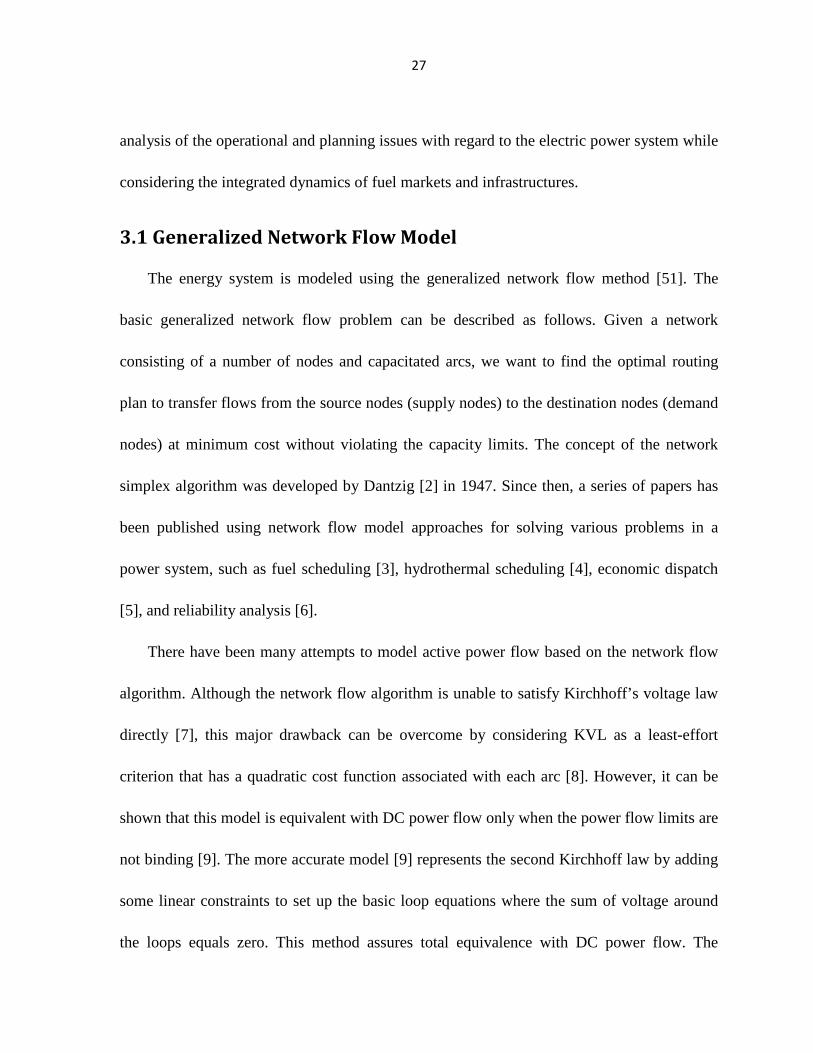
3.1 Generalized Network Flow Model
The energy system is modeled using the generalized network flow method [51]. The
basic generalized network flow problem can be described as follows. Given a network
consisting of a number of nodes and capacitated arcs, we want to find the optimal routing
plan to transfer flows from the source nodes (supply nodes) to the destination nodes (demand
nodes) at minimum cost without violating the capacity limits. The concept of the network
simplex algorithm was developed by Dantzig [2] in 1947. Since then, a series of papers has
been published using network flow model approaches for solving various problems in a
power system, such as fuel scheduling [3], hydrothermal scheduling [4], economic dispatch
[5], and reliability analysis [6].
There have been many attempts to model active power flow based on the network flow
algorithm. Although the network flow algorithm is unable to satisfy Kirchhoff’s voltage law
directly [7], this major drawback can be overcome by considering KVL as a least-effort
criterion that has a quadratic cost function associated with each arc [8]. However, it can be
shown that this model is equivalent with DC power flow only when the power flow limits are
not binding [9]. The more accurate model [9] represents the second Kirchhoff law by adding
some linear constraints to set up the basic loop equations where the sum of voltage around
the loops equals zero. This method assures total equivalence with DC power flow. The

28
advantage of this algorithm, regarding DC power flow algorithms, is explicit representation
of branch flows. Consequently, transmission limits can be promptly imposed and
transmission losses can be expressed in the objective function. The proposed model
represents KVL in a similar way by adding some variables and linear constraints.
Fig. 3.1 is an example of a typical network, which is composed of supply and demand
nodes together with directed arcs connecting them. There are four properties associated with
each arc: cost coefficient c, flow efficiency η, lower bound emin, and upper bound emax.
Piecewise linearization can be performed to deal with the convex quadratic cost function of
the arc flow. Then a single arc can be substituted by multiple arcs, each representing one
segment of the piecewise linear function. For nodes that represent facilities that add cost or
losses to the flow, such as fuel production facilities and power plants, one node is split into a
pair of nodes with arcs connecting them. The cost and/or loss generated by these facilities
can be expressed in the arc.
Fig. 3.1. A typical network flow diagram.

29
Fig. 3.2. Representing a generator’s marginal cost curve
In Fig. 3.2, when the generator is bidding at its marginal costs, the three arcs represent
the generator’s energy bidding curves. As the objective of the production cost simulation
problem is the minimization of total production cost, arc 1 will first be used to transfer the
energy flow due to its low cost. When the demand goes higher and flow in arc 1 reaches it
limit, arc 2 will then be used, followed by arc 3. In the same manner, the cost/efficiency
associated with transmission lines and the generating units can be captured.
In the proposed model, both the electric system and fuel system are considered in order
to capture the fuel cost of generators directly. In the proposed model, one generator node is
split into a pair of generator nodes so that operating constraints and operation and
maintenance (O&M) costs can be expressed as the properties of the arc connecting the two
nodes. Generator maximum and minimum output limits are enforced by constraining the
energy flow between the paired generator nodes.

30
3.2 Combining DC Power Flow Model with GNF Model
3.2.1 System Formulation
In this minimal cost network flow model, the interest is to optimize the flows of fuel and
electric energy in an integrated network in the most economical way. Fuel production,
transportation and storage costs and losses, generation costs, and transmission costs and
losses are included in the model.
Fig. 3.3. The interactions between fuel transportation system and electric transmission system
The objective function, which is to be minimized, is the sum of the costs associated with
all kinds of flows in the network. The prices of different kinds of fuels at the fuel production
side, such as wellhead natural gas prices and spot price of coal in different coal-producing
regions, are included in the cost property of transportation arcs. Equation (3.2) represents that
for each node, the sum of flows into the node minus the flows out of the node equals the
demand (or supply if negative) of the node. For the electric transmission system, Kirchhoff's
first and second laws are fulfilled by Equations (3.3) and (3.4). Arc flows and power angles

31
must be within constraints, as is shown in Equations (3.5) and (3.6). For the fuel
transportation network, arc flows should be larger than or equal to zero, whereas in the
transmission network, arc flow can be negative to account for the bidirectional nature of the
power flow. Each generation nodes is split into a pair of nodes and an arc linking them in
order to account for the operation and maintenance (O&M) cost of the power plant as well as
its generation capacity.
Minimize ( , )
Z ( ) ( )ij ijt T i j Mt Mf
c t e t∈ ∈ ∪
=∑ ∑ (3.1)
Subject to
( ) ( ) ( ),ij ij ij ji k
e t e t d tη∀ ∀
− =∑ ∑ ,j Nf t T∀ ∈ ∀ ∈ (3.2)
( ) ( ( ) ( )) 0,ij ij i je t b t tθ θ− − = ( , )i j Mt∀ ∈ (3.3)
( ) ( ( ) ( )) ( ),i i
ji ji ij i j ij G j B
e t b t t d tη θ θ∈ ∈
− − =∑ ∑ , ( , )i Nt i j Mt∀ ∈ ∀ ∈ (3.4)
.min .max( ) ,ij ij ije e t e<= <= ( , ) ( )i j Mt Mf∀ ∈ ∪ (3.5)
,iπ θ π− <= <= i Nt∀ ∈ (3.6)
3.2.2 Nodal Prices
As a byproduct of the model, marginal prices of nodes in both the fuel transportation and
storage network and the electric network can be calculated. The term nodal price is defined
as the change in total cost that arises when the quantity produces changes by one unit. The
objective function and equation (3.1)--(3.5) can be combined to form the Lagrange function
L using Lagrangian multipliers (which are interpreted as dual prices or shadow prices). The

32
Lagrangian multiplier is the rate of change in objective value as a function of constraint
variable. In the production cost model, when optimal solutions are obtained, Lagrangian
multipliers are indicators of the costs of supplying/consuming one more unit of energy. In
electric system, this means the cost of serving the next MW of load at a specific node. In fuel
system, Lagrangian multiplier is the cost of transporting/storing the next unit of fuel at a
specific location. We use the term nodal prices for these marginal costs in both systems.
L= ( , )
( ) ( )ij ijt T i j Mt Mf
c t e t∈ ∈ ∪∑ ∑ + ( )j
t T j Nf
tλ∈ ∈∑∑ ( ) ( ) ( )ij ij jk j
i k
e t e t d tη∀ ∀
− + + ∑ ∑
+( , )
( ) ( ) ( ( ) ( )) ( )i i
i ji ji ij i j it T i j Mt j G j B
t e t b t t d tγ η θ θ∈ ∈ ∈ ∈
− + − +
∑ ∑ ∑ ∑ +( , )
( )ijt T i j Mt
tα∈ ∈∑ ∑
( ) ( ( ) ( ))ij ij i je t b t tθ θ − − + .min( , )
( ) ( )ij ij ijt T i j Mt Mf
t e e tδ∈ ∈ ∪
− ∑ ∑ +
.max( , )
( ) ( )ij ij ijt T i j Mt Mf
t e t eµ∈ ∈ ∪
− ∑ ∑ + [ ]( ) ( )ij it T i Nt
t tβ π θ∈ ∈
− −∑∑ + [ ]( ) ( )ij it T i Nt
t tω θ π∈ ∈
−∑∑
(3.7)
The relationship between linked nodes can be derived by applying
Karush-Kuhn-Tucker(KKT) first-order optimal conditions to the above Lagrangian function.
When an optimal solution to the optimization problem is obtained, the first-order derivatives
of Lagrange function L with respect to each decision variable ( )ije t should be zero. Thus, the
relationship between nodal prices of nodes that are connected by ( )ije t can be shown.
When( )ij Mf∈ , the nodal prices between two linked nodes i and j are given in the
following equation:
( ) ( ) ( ) ( ) ( ) 0( ) ij i ij j ij ij
ij
Lc t t t t t
e tλ η λ δ µ
∂= + − − + =
∂ (3.7)

33
If the arc flow constraints are not binding, ( )ij tδ and ( )ij tµ are both zero. If we assume the
energy flow is costless and lossless, then( )i tλ = ( )j tλ . Under normal conditions, the difference
between nodal prices of two connected nodes is decided by whether the arc flow is congested,
the cost of transferring the energy and the efficiency of energy flow. The nodal prices of fuel
production nodes are given as the prices of raw fuel resources at wellhead/coal mines. Then
according to equation (3.7), nodal prices of other nodes in fuel system can also be obtained.
The connections between fuel system and electric system are arcs that connect pseudo
generator nodes to generator nodes. Equation (3.7) also applies to energy flows in these arcs,
so we can get nodal prices of generator nodes.
When( )ij Mt∈ , the nodal prices between two linked nodes i and j are given in the
following equation:
( ) ( ) ( ) ( ) ( ) 0( ) i j ij ij ij
ij
Lt t t t t
e tλ γ α δ µ
∂= − + − + =
∂
(3.8)
In this model, in electric system, neither line losses nor transmission costs is considered.
So transmission line congestion is the only factor for nodal prices differences between two
connected nodes. The presence of difference between nodal prices means the generation at
lower-priced locations cannot be transferred to high-priced locations due to flow constraints.
3.3 Numerical Example
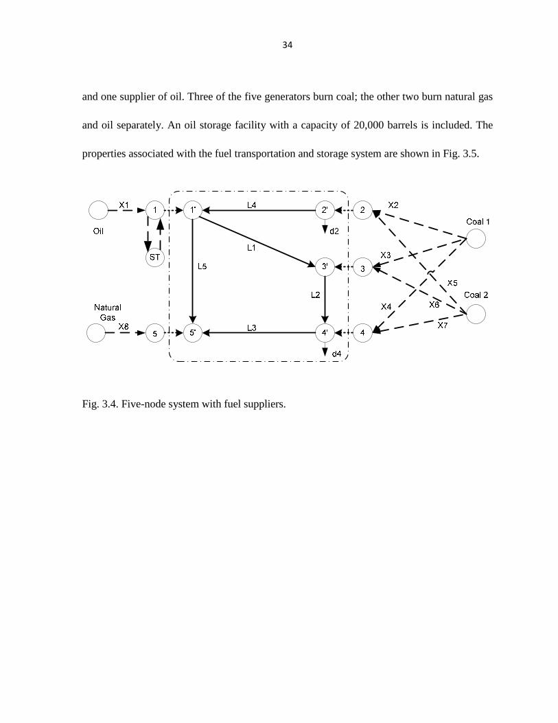
To evaluate the methodology presented before, a five-node system has been considered.
In the system shown in Fig. 3.4, there are two suppliers of coal, one supplier of natural gas,
34
and one supplier of oil. Three of the five generators burn coal; the other two burn natural gas
and oil separately. An oil storage facility with a capacity of 20,000 barrels is included. The
properties associated with the fuel transportation and storage system are shown in Fig. 3.5.
Fig. 3.4. Five-node system with fuel suppliers.

35
Fig. 3.5. Fuel transportation and storage system.
The five-bus system is tested for a period of 52 weeks to analyze the mid-term operation
characteristics. In order to encapsulate the load duration characteristics of the demand in the
algorithm, load is represented as weekly load duration curves (LDCs). An LDC plots the
number of hours (percentage of hours per year) that the load equals or exceeds a given level
of demand. In order to reduce the computation time, the LDC is simplified to have three
levels of load that represent high, medium and low demand. There are variations with
wellhead oil and natural gas prices, with peak price appearing in the middle of the year (see
Figure 5). Coal price is determined mainly by long-term contracts and coal supply is less
dependent on import than oil and natural gas, so coal price tends to be stable. This estimation
is in line with historical data of coal prices from EIA.

36
The flows of the test system under five scenarios were calculated, as shown in table 1.
The “No DC OPF” scenario uses the original generalized network flow model and one set of
the multiple solution sets is shown. The “Base case” scenario considers a transmission
system without any flow constraints. In scenario “Case 1”, a 100 MW flow constraint is
applied on line L4. In scenarios “Case 2”, load on node 4 was increased to 1600 MW. In
scenario “Case 3”, the flow limit in line X5 is 200 ton (per hour).
Table 3.1 Optimal results of five scenarios

37
Fig. 3.6. Oil and natural gas prices
Fig. 3.7. Oil Storage level
Fig. 3.6 shows the oil storage level for the 52-week term. The storage level is very high in
the beginning, when oil price is in a low level; whereas when oil price increases, the storage
level drops accordingly.
5 10 15 20 25 30 35 40 45 50
15
20
25
30
Week
$/ba
rrel
Wellhead oil and natural gas prices
5 10 15 20 25 30 35 40 45 503
3.5
4
4.5
5
5.5
$/M
cf
5 10 15 20 25 30 35 40 45 500
50
100
150
200
Week
100
Bar
rel
Oil storage level

38
Fig. 3.8. Generation levels
Fig. 3.9. Locational marginal prices
Fig. 3.8 shows the weekly average generation levels of generators over 52 weeks.
Coal-fired power plants generally have higher fixed costs and lower operating cost than
gas-fired and oil-fired plants, so they run all the time (base-load plants). Gas-fired power
plants, on the contrary, have higher operating costs and lower fixed costs, so they only run
0 5 10 15 20 25 30 35 40 45 500
1
2
3
4
5
6
7
8
9
10
11
Week
100
MW
Weekly Average Generation level
V1
V2
V3V4
V5
0 5 10 15 20 25 30 35 40 45 5010
15
20
25
30
35
40
45
50
Week
$/
MW
h$
/ M
Wh
$/
MW
h$
/ M
Wh
Weekly Average LMP
Gen 1
Gen 2
Gen 3
Gen 4
Gen 5
Load 2
Load 4

39
when load is very high. Fig. 3.9 presents the weekly average LMPs of each bus and load.
Although LMPs of oil-fired and gas-fired plants are higher, they only operate for a short time
each week, so the average LMPs of two demands are only a little higher than the highest
coal-fired power plant. What is more, the storage facility helps to reduce the oil price by
saving the cheaper oil in the beginning of the year for later use.
Fig. 3.10. Branch flows (with DC power flow)
0 5 10 15 20 25 30 35 40 45 50-10
-8
-6
-4
-2
0
2
4
6
8
10
Week
100
MW
Weekly Average Branch Flows (with DC power flow )
L1
L2
L3L4
L5

40
Fig. 3.11. Branch flow (no DC power flow)
A comparison of branch flows optimized by models with and without DC power flow is
shown in Fig. 3.10 and Fig. 3.11. There is a 1,000 Mw constraint on each transmission line in
both cases. Fig. 3.11 shows the extreme condition where no loss or cost is considered. The
reason for differences between the two cases is that in the first case, DC power flow function
is not incorporated, so the flows in the transmission system only comply with KCL, but not
KVL.
Table 3.2 Generators’ real power output and branch flows (week 2 low demand hours).
Table 3.2 shows the optimal solutions generated by the models with and without DC
power flow. We can see that when DC power flow is not incorporated, active power flows in
the direction of 1→5→4→3→1, which violates KVL in that the sum of price drop in one
0 5 10 15 20 25 30 35 40 45 50-10
-8
-6
-4
-2
0
2
4
6
8
10
Week
100
MW
Weekly Average Branch Flows (No DC power flow)
L1
L2
L3L4
L5

41
loop is not zero. Consequently, the flow generated in this model won’t happen in the real
system.
Let’s take a look at network flow model without DC power flow. There is no cost or loss
associated with the branch flows, so for the overall optimization problem, as long as branch
flows can satisfy KCL for buses 1−5, the value won’t affect the optimal value of the
objective function and other variables. So we can assume that the generators’ active power
output is given, and the following equations can be made to get branch flow.
" BP � # (3.9)
$%%%&'()*'()*'()*'()*'()*+
,,,-
.
$%%%&'1'2'3'4'5+
,,,-
.
$%%%&'(45'(45'(45'(45'(45+
,,,- (3.10)
Where "=
$%%%& 1 0 0
0 0 071 1 0
010
100
0 0
710
171
00
071+
,,,-, BP =
$%%%&'1'2'3'4'5+
,,,-, and # =
$%%%& 8182 7 92
8384 7 94
85 +,,,-.
V1−V5 are the generators’ real power output. d2 and d4 are loads in buses 2 and 4, which
are known. The determinant of " is zero. According to Cramer’s rule, if the right-hand side
of the equation is not zero and the determinant of coefficient matrix is zero, the system has
no unique solution. So there will be multiple solutions to the same equation and the branch
flows generated from the model can be any one of the multiple solutions, which explains why
the branch flows change so violently over time. For example, in Table 3.2, the branch flows
in both cases satisfy Equation 3.9, yet they are totally different. In larger transmission

42
systems, the coefficient matrices tend to be sparse, so their determinants are usually zero.
Consequently, for a given level of the generators’ real power output, there might be multiple
sets of branch flows that can satisfy equation (3.9) and the solution generated by the model
can be either one of them.
For the network model with DC power, we can also form equations to get branch flows.
#: = (; < ")=>′?@A# (3.11)
#: is a vector of branch flows. D is a diagonal matrix with the diagonal elements in row k,
column k contains the negative of susceptance of the BCD branch. A is the M<(N-1)
node-arc incidence matrix. B is of dimension (N-1)<(N-1). P is the vector of nodal injections
for buses 2,…,N. Apparently, given a certain P, there will be a unique #:.
If costs or losses are associated with branch flows, the branch flows in the second case
(without DC power flow) are included in the objective function, and then the optimal
solution would be the one that minimizes the overall cost of the system. However, there is no
guarantee that the branch flow solution will comply with KVL. When modeling larger
systems, e.g., western interconnection, the difference with branch flow solutions will still
occur in that, after all, KVL is not represented by the model without DC power flow. The
solution derived from this model might be optimal the least-cost way but physically
impossible. The differences with branch flows will in turn affect the optimal solutions of the
other variables and the overall objective function if cost or losses is considered. For decision
makers, accurate active power flow solutions will give them a better idea of transmission line

43
congestion level so that they can arrange their operation plans accordingly. What is more,
LMP will not be right if it’s based on inaccurate branch flows.
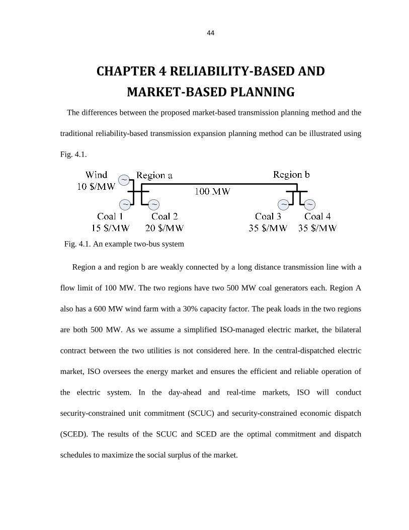
44
CHAPTER 4 RELIABILITY-BASED AND
MARKET-BASED PLANNING
The differences between the proposed market-based transmission planning method and the
traditional reliability-based transmission expansion planning method can be illustrated using
Fig. 4.1.
Fig. 4.1. An example two-bus system
Region a and region b are weakly connected by a long distance transmission line with a
flow limit of 100 MW. The two regions have two 500 MW coal generators each. Region A
also has a 600 MW wind farm with a 30% capacity factor. The peak loads in the two regions
are both 500 MW. As we assume a simplified ISO-managed electric market, the bilateral
contract between the two utilities is not considered here. In the central-dispatched electric
market, ISO oversees the energy market and ensures the efficient and reliable operation of
the electric system. In the day-ahead and real-time markets, ISO will conduct
security-constrained unit commitment (SCUC) and security-constrained economic dispatch
(SCED). The results of the SCUC and SCED are the optimal commitment and dispatch
schedules to maximize the social surplus of the market.

45
If there were no transmission limit on the transmission line, the low-cost generators in
region a will substitute the high-cost generators in region b so that the total production costs
in the system are minimized at all hours. There will be a 500 MW flow in the transmission
system during the peak hours. However, due to transmission line thermal limit and other
reliability reasons, ISO needs to make sure that the flow limits will not be violated. Thus, a
rather than allowing 500MW flow during the peak hours, the maximum flow on the
transmission line is 100MW. Apparently, the test system has a much higher production cost
now than that of the case with no transmission limits.
In the electric system, there are generally two ways to maintain the transmission flow
within the defined set limit. When there is an overload in the transmission network, system
operator can conduct TLR (through curtailment of scheduled transactions), market
re-dispatch (by means of binding elements), or both, to maintain system reliability. While
congestions as the result of contingencies and dispatches need to be taken care of
immediately, most of the congestions only reflect proper system management with reliability
regions and do not mean requirement for system expansion. There are generally two
categories of transmission congestions:
1) Most of the time, when congestion occurs, there are plenty of other generation
resources and mitigation options available. Simply shifting the generation supply among the
available generator and reducing the demand via demand-side management can solve the

46
congestions. In this kind of situation, the system is operating in a less-economical way
compared to the non-congested system.
2) Alternatively, in some rare cases, transmission thermal limits are reached and there is
either no generation resources readily available for dispatch or generation resources are
sufficient system-wide but limited by transmission bottlenecks. As the result of this kind of
congestions, system operators have limited mitigation plans except for curtailing the load.
The former category of congestions might not justify the needs for transmission system
expansion from reliability point of view, the later, however, violates system reliability
criteria set by FERC and is a clear indicator for system expansion needs.
In the test system, reliability-based transmission planning will not expand transmission
system because there is no load curtailment during peak hours under N-1 contingency
conditions. However, as the inter-regional transmission line is heavily congested, LMP in
region b is much higher than region a. Although region a has excess low-cost energy, it
cannot be transferred to region b because of transmission bottleneck. The consumers in
region b need to pay a much higher price for electricity. Due to the congestion, the total
load payments in the two regions are higher than the total amount of money that generators
receive. The difference between the revenues collected and costs incurred is called
merchandising surplus or congestion cost. The appearance of large merchandising surplus
means there is social surplus loss in the whole market, which indicates that the system is
operating inefficiently [52]. Unlike reliability-based transmission planning method, the

47
market-based transmission planning model will consider investing new transmission lines
between the two regions to relieve the congestions, promote competition and enhance the
efficiency of the market. Similarly, reliability-based planning would not build HVDC
transmission from the US Midwest, where energy prices are low, to the US East Coast, where
energy prices are high, but market-based planning would.
4.1 Reliability-Based Transmission Expansion Planning
4.1.1 Overall Formulation
The objective of traditional transmission expansion planning is to find the least-cost
alternative to serve the load demand of all existing and future customers reliably. Capital
investments are justified on the grounds of reliability requirements. In reliability-based
transmission planning, the investment decision is made based on the operating conditions
during the system’s peak-load hours and under various contingencies. Such a planning effort
is based upon load/generation forecasts and the lead times required to implement resource
and transmission investment decisions. In today’s ISO/RTO markets, such planning
processes are conducted both by regional transmission organizations and/or by transmission
companies. When ISO/RTOs are conducting reliability-based planning, the planning are done
at a regional level with the active participation from generation and transmission companies,
load serving entities, state regulators, and many other market participants. Based on various
reliability criteria (power flow, power transfer limits, contingency analysis for steady-state,

48
dynamic, voltage, and small-signal stability) and economic assessment of investment costs, a
set of transmission investment plans are created. In this paper, an N-1 contingency reliability
criterion is adopted. The N-1 contingency criterion means that the system should withstand
an outage of one major element, such as a line, generator or transformer. In this paper, we
only consider transmission line outages. This is a reasonable assumption considering that
most major blackouts are transmission based, and that transmission lines are vulnerable to
various disturbances.
4.1.2 Master Problem
The master problem is the decision making problem. The objective function is the
minimization of the present value of investment costs. Constraint (4.2) is the cut from the
slave problem, which indicates that there are violations (loss of load) in iteration k under wth
contingency. Constraint (4.3) updates the total number of each line at time t considering the
lead time of investments. Both the number of lines to be built each year and the total number
of lines are subject to constraints, as shown in constraints (4.4) and (4.5).
(1 ) ( )
( ) '
tMin r I m tij ij
t T ij Mn
−+∑ ∑∈ ∈
(4.1)
subject to
( )( ( ) ( )) 0 ( ) '
kw k kwt n t n t Zij ij ij
t T ij Mnδ − + ≤∑ ∑
∈ ∈ (4.2)
( ) ( 1) ( )n t n t m t aij ij ij
= − + −
(4.3)

49
0 ( ) m t mij ij
≤ ≤ (4.4)
0 ( ) n t nij ij
≤ ≤ (4.5)
where ijδ is the sensitivity of the optimum value Z with respect to the decision variable nij
given by Romero and Monticelli [53]:
( ) ( ( ) ( ))( ( ) ( )) t B t t t tij ij i j i j
δ θ θ λ λ= − − − (4.6)
4.1.3 Slave Problem
In the slave problem, the impact of the transmission expansion plan is assessed under
worse-case scenarios to ensure the system is designed and operated to a certain level of
reliability. As the N-1 contingency criterion is adopted, the transmission investment must
ensure that, under the loss of any single equipment, the system won’t have any load
curtailment during peak hours throughout the planning horizon. Thus, each slave problem is
a feasibility check problem, which checks the reliability of the system under an N-1
contingency. In each iteration, there are w sub-problems, each representing the outage of one
major element in the system. rj(t) is the slack variable in constraint (4.2), which balances the
total energy input and total energy output for node j at time t. If rj(t) > 0, it means that there
is not enough power to supply the electric demand. In this case, a portion of the demand is
not satisfied, which, in other words, means a violation occurs. Zw is the sum of all slack
variables, and if Zw > 0, it means that violations occur during wth contingency and the load
cannot be satisfied at some time. Thus, a feasibility cut is added to the master problem in
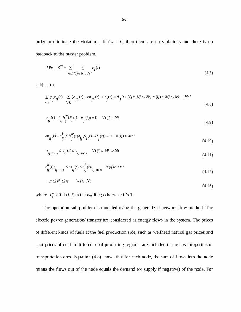
50
order to eliminate the violations. If Zw = 0, then there are no violations and there is no
feedback to the master problem.
( )
'
wMin Z r tjt T j N N
= ∑ ∑∈ ∀∈ ∪
(4.7)
subject to
( ) ( ( ) ( )) ( ) ( ), , ( ) 'e t e t en t r t d t j Nf Nt ij Mf Mt Mnij ij jk jk j j
i kη − + + = ∀ ∈ ∪ ∀ ∈ ∪ ∪∑ ∑
∀ ∀ (4.8)
( ) ( ( ) ( )) 0 ( )we t b h t t ij Mtij ij ij i j
θ θ− − = ∀ ∈ (4.9)
( ) ( ) ( ) ( ( ) ( )) 0 ( ) 'k wen t n t h t b t t ij Mn
ij ij ij ij i jθ θ− − = ∀ ∈
(4.10)
( ) ( )
.min .maxe e t e ij Mf Mtij ij ij
≤ ≤ ∀ ∈ ∪ (4.11)
( ) ( ) ( ) ( ) '
.min .maxk k
n t e en t n t e ij Mnij ij ij ij ij
≤ ≤ ∀ ∈ (4.12)
i Nt
iπ θ π− ≤ ≤ ∀ ∈
(4.13)
where wijh is 0 if (i, j) is the wth line; otherwise it’s 1.
The operation sub-problem is modeled using the generalized network flow method. The
electric power generation/ transfer are considered as energy flows in the system. The prices
of different kinds of fuels at the fuel production side, such as wellhead natural gas prices and
spot prices of coal in different coal-producing regions, are included in the cost properties of
transportation arcs. Equation (4.8) shows that for each node, the sum of flows into the node
minus the flows out of the node equals the demand (or supply if negative) of the node. For

51
the electric transmission system, Kirchhoff's first and second laws are fulfilled by constraints
(4.9), (4.10) and (4.11). Arc flows and power angles must be within constraints, as shown in
constraints (4.11), (4.12) and (4.13). Constraint (4.11) exerts constraints on flows in the
existing network; Constraint (4.12) exerts constraints on flows in the potential lines. If no
new line is installed in time t, nij(t) is 0, then enij(t) is also 0. For the fuel transportation
network, arc flows should be larger than or equal to zero, whereas in the transmission
network, arc flow can be negative to account for the bidirectional nature of the power flow.
4.1.4 Iteration Procedures
Fig. 5 shows the iteration procedures for the reliability-based transmission planning
model. At the beginning of the planning process, the master problem is solved without any
cut (constraint (4.2)). Then the investment decisions about when, where and which lines
should be built are sent to the slave problems. The slave problems check the adequacy of the
electric supply under various contingencies for the whole planning horizon. If there is a
violation in any slave problem, a feasibility cut is generated and added to the master problem.
The iterations between the master problem and slave problem continue until there are no
violations in all of the slave problems.

52
1 1,
k kZijδ
knij
2 2,
k kZijδ
knij
,kw kw
Zijδ
Fig. 4.2. Iterations between master and slave problems in the reliability-based planning
4.2 Market-Based Transmission Expansion Planning
4.2.1 Overall Problem
Market-based transmission investment assumes that an efficient investment might bring
sufficient economic benefit when the transmission system has a high level of congestion. In
this paper, we assume ISOs will conduct the market-based transmission planning study for
the whole system in order to find the profitable investment opportunities for companies or
individual investors that are interested. By doing so, ISOs ensure the efficient operation of
the whole electric market.
According to economic theories, social surplus is a good indicator of how well the
market is working. Thus, social surplus should be used to quantify the economic benefits that
network expansions bring. From the social welfare perspective, a market-based transmission
investment is justified if the total social surplus increase caused by the investment is higher

53
than the cost of the investment itself. However, the two values are hard to compare in that
while investment cost is incurred at a certain time and can be considered as present value at
the beginning of the planning horizon, social surplus occurs at every time step. So in the
slave problem, social surplus must be calculated at every hour throughout the planning
horizon or a way to approximate this process must be found.
4.2.2 Market Structure and Operation
In this paper, the ISO-managed day-ahead market is considered. In the ISO-managed
day-ahead market, all transactions are carried out by an ISO which clears the market for both
the generation companies (GenCos) and load-serving entities (LSEs) [54]. The responsibility
of an ISO is to ensure the reliable and efficient operation of the wholesale electricity market.
The objective of the LSEs (buyers) is to ensure the highest possible net earning each day by
buying electric power from the day-ahead market and selling it in the retail electric market.
The objective of GenCos (sellers) is to acquire the highest possible net earning each day by
selling electric power in the day-ahead market.
At the beginning of each day, each GenCo submits to the operator an incremental cost
and the amount of energy it is willing to sell and each LSE submits to the operator a
decremental cost and the amount of energy it is willing to buy. After receiving offers and
bids for the next day, the ISO then conducts an optimal power flow based on offers/bids and
determines the hourly dispatch schedules and locational marginal prices (LMPs). Each
GenCo gets paid by the LMP it receives and each LSE pays the LMP for the electric power it

54
purchases. In this paper, all generators are bidding according to their marginal cost curves, so
strategic bidding is not considered.
The generator’s cost is generally comprised of two parts: the fuel cost and the O&M cost.
The fuel cost is decided by the price of fuel at its production site, e.g., coal mines, gas well,
etc., and the costs to transport and store the fuel. In our generalized network flow model, fuel
cost can be expressed as the cost of transferring the flows (fuel) from the supply nodes to the
generator. The O&M cost is generalized to have not only the regular maintenance, repair, and
spare parts costs, but also fixed costs such as insurance, return to stockholders, administration
costs, etc. The marginal cost of generators normally grows with the increase of power output.
The marginal cost curves can usually be adequately approximated using piecewise linear
functions. Fig. 4.3 shows the generator marginal cost curve as well as incremental fuel cost
curve and incremental O&M cost curve. The marginal fuel cost can be described using a step
function, while the incremental O&M cost increases linearly as generation output increases.
As can be seen in the figure, when the generator output is x MW, the production cost is the
sum of areas S1 and S2, which are the total fuel cost and total O&M cost respectively.
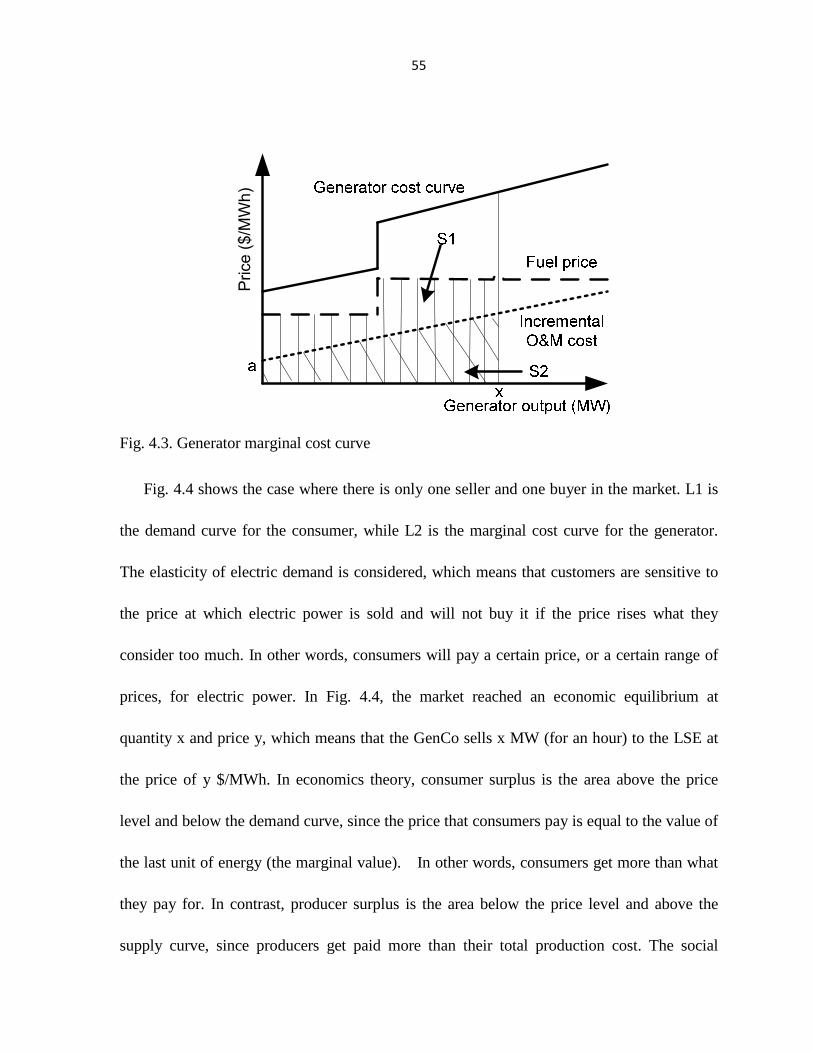
55
Price ($/MWh)
Fig. 4.3. Generator marginal cost curve
Fig. 4.4 shows the case where there is only one seller and one buyer in the market. L1 is
the demand curve for the consumer, while L2 is the marginal cost curve for the generator.
The elasticity of electric demand is considered, which means that customers are sensitive to
the price at which electric power is sold and will not buy it if the price rises what they
consider too much. In other words, consumers will pay a certain price, or a certain range of
prices, for electric power. In Fig. 4.4, the market reached an economic equilibrium at
quantity x and price y, which means that the GenCo sells x MW (for an hour) to the LSE at
the price of y $/MWh. In economics theory, consumer surplus is the area above the price
level and below the demand curve, since the price that consumers pay is equal to the value of
the last unit of energy (the marginal value). In other words, consumers get more than what
they pay for. In contrast, producer surplus is the area below the price level and above the
supply curve, since producers get paid more than their total production cost. The social

56
surplus is the sum of consumer surplus and producer surplus, which is essentially area S3
(S4-S1-S2). For a market that has multiple participants, we can get the total social surplus on
the figure of the cumulative demand curve and cumulative supply curve.
Fig. 4.4. Supply- and Demand-side bidding curves
In many economic planning models, in order to capture the fundamental economic
benefits of circuit installations, various expansion criteria are defined, such as production
costs [5], flatness of price profile [1], congestion rent [4], redispatch cost, etc. In this paper, a
day-ahead bulk electric market is considered. According to [8], the objectives of the electric
market framework are promoting market efficiency, lowering energy delivery cost, securing
system reliability, mitigating significant market power and increasing the choices offered to
market participants. Thus, social surplus is used as the market-based expansion criterion as it
is the primal measure of the efficiency of a market. When there are congestions in the

57
transmission grid, less expensive energy cannot be freely transferred in the market, which
causes some valuable resource to remain unused. What is more, the congestions in the system
will hamper the full extract of all possible surpluses as price-sensitive demand might be
curtailed as the result of an insufficient supply of less expansive energy. In order to enhance
market efficiency, we need to invest in new transmission lines to eliminate or reduce the
level of congestion in the system. The idea of market-based transmission expansion planning
is based on the trade-off between the investment costs and the induced increase in social
surplus.
4.2.3 Master Problem
In the planning problem, while generally more circuit expansions will promote the
efficient operation of the electric market and increase the social surplus, they also means
more investment cost. The master problem tries to find a trade-off between high investment
cost and increase in social surplus. The objective function is the minimization of social costs
(investment costs minus social surplus), which is the same as maximization of social surplus
minus investment costs.
(1 ) ( ) ( ) '
tMin r I m t Zij ij
t T ij Mn
− ∗+ +∑ ∑∈ ∈ (4.14)
Subject to
0Z∗ ≤ (4.15)
( )( ( ) ( ))( ) '
k k kZ t n t n t Zij ij ij
t T ij Mnδ∗ ≥ − +∑ ∑
∈ ∈ (4.16)

58
( ) ( 1) ( )n t n t m t aij ij ij
= − + − (4.17)
0 ( ) m t m
ij ij≤ ≤
(4.18)
0 ( ) n t nij ij
≤ ≤ (4.19)
where Zk is the optimal value of the slave problem in the kth iteration and ijδ can also be
expressed as (4.6).
4.2.4 Slave Problem
The slave problem tries to minimize the social cost plus loss of load penalties. The major
differences between the slave problem in market-based transmission planning and that of
reliability-based transmission planning are that: (1) The former tries to minimize the social
costs by conducting optimal power flow (OPF), while the latter tries to check if there is any
load curtailment; (2) The former needs to calculate the economic value introduced by circuit
additions throughout the planning horizon, which means it needs to optimize the operations
of system either chronologically or under a set of typical conditions that can approximate the
hour-by-hour load levels, while the latter only needs to check violations during peak-load
hours of each year; (3) The former is a quadratic programming problem as the double-sided
bidding is considered, while the latter is a linear programming problem; (4) There is only one
slave problem in market-based planning, while there are w slave problems in
reliability-based planning, each representing a contingency in the system; and (5) The slave
problem in market-based planning will generate an optimality cut to the master problem,

59
while one slave problem in reliability-based planning will generate a feasibility cut only
when its optimal objective value is higher than zero.
(1 ) ( ( ) ( ) ( ) ( )( , )
( ( )) ( ( )))( , ) ( , )
tMin Z r c t e t lol t r tij ij j
t T i j Mf Mt j Nf Nt
S e t D e tij ij ij ij
i j Mg i j Md
−= + +∑ ∑ ∑∈ ∈ ∪ ∀ ∈ ∪
+ −∑ ∑∈ ∈
(4.20)
Subject to
( ) ( ( ) ( )) 0 ( )e t b t t ij Mtij ij i j
θ θ− − = ∀ ∈ (4.21)
( ) ( ) ( ( ) ( )) 0 ( ) 'ken t n t b t t ij Mnij ij ij i j
θ θ− − = ∀ ∈ (4.22)
( ) ( ) ( ) ( ) 'k kn t e en t n t e ij Mnij ij ij ij ij
≤ ≤ ∀ ∈ (4.23)
( ) ( ( ) ( )) ( ) 0 ,
( ) ', ( ) '
e t e t en t r t j Nf Ntij ij jk jk j
i k
ij Mf Mt Mn jk Mf Mt Mn
η − + + = ∀ ∈ ∪∑ ∑∀ ∀
∀ ∈ ∪ ∪ ∀ ∈ ∪ ∪ (4.24)
( ) ( ).min .max
e e t e ij Mf Mtij ij ij
≤ ≤ ∀ ∈ ∪ (4.25)
i Nti
π θ π− ≤ ≤ ∀ ∈ (4.26)
As shown in Fig. 4.3, if we assume the intercept and slope of the incremental O&M cost
curve for( , )i j Mg∈ are aij and sij respectively, the total O&M cost Sij(eij(t)) is:
2( ( )) ( ) ( ) / 2S e t a e t s e tij ij ij ij ij ij
= + (4.27)
In the same way, if we assume the intercept and slope of consumer bidding curve for
( , )i j Md∈ are pij and qij respectively, the total consumer benefit Dij(eij(t)) is:

60
2( ( )) ( ) ( ) / 2D e t p e t q e tij ij ij ij ij ij
= + (4.28)
In order to encapsulate the load duration characteristics of the demand, load is
represented as yearly load duration curves (LDCs). An LDC plots the number of hours
(percentage of hours per year) that the load equals or exceeds a given level of demand.
Compared to simulating the system chronologically, LDC helps to reduce the computation
time.
4.2.5 Iteration Procedures
The overall problem is solved by iterating between the master and the slave problem, as
shown in Fig. 4.5. In each iteration, the master problem generates a set of investment
decisions and passes them to the slave problem. The slave problem simulates the operation of
the market and gets new values of Z and δij using the solution obtained in the master problem.
Then the Benders optimality rule is used to check whether the optimal solution is achieved. If
not, a cut will be added to the master problem and the next iteration gets started.
knij
,k k
Zijδ

61
Fig. 4.5. Iterations between master and slave problems in the market-based planning
4.3 Numerical Example
4.3.1 5-bus System
To evaluate the methodology presented before, a 5-bus system has been considered. Fig.
4.6 shows the network diagram of the integrated energy system, which has three integrated
gasification combined cycle (IGCC) power plants, one natural gas combined cycle (NGCC)
power plant and an oil-fueled power plant. The fuel subsystem which includes four fuel
suppliers and eight fuel transportation lines is also considered. Fuel transportation arcs X5
and X6 do not exist at the beginning of the planning horizon. They will come into use at year
2 and year 5, respectively.
Fig. 4.6. Five-bus system with four fuel suppliers
The expected values of the natural gas price and oil price increases at a rate of 4% per
year, while the coal price has a growth rate of 2% per year. The coal price is determined
mainly by long-term contracts, and coal supply is less dependent on import than oil and

62
natural gas, so the coal price tends to be stable. This estimation is consistent with historical
data of coal prices from the Energy Information Administration (EIA).
The market-based transmission expansion planning is carried out on this system for a
planning horizon of 10 years. In order to reduce the computation time, yearly LDCs are used.
Investment decisions are made at the beginning of each year.
Reliability-based transmission expansion planning considers the N-1 contingencies and
generates investment decisions to ensure the system has no loss of load even in peak hours.
The reliability-based planning method is also carried in this system with the same load
conditions.
Table 4.1. Investment plans made by the two planning methods
A comparison between the results of the two planning methods is shown in Table 4.1. In
order to reduce the investment cost, reliability-based planning will not invest new lines until
they are needed. Because of the discount rate, the later the investment is made, the smaller
the present value of the investment is. Market-based planning, however, tries to find the
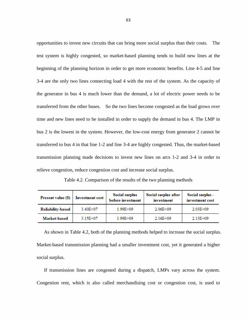
63
opportunities to invest new circuits that can bring more social surplus than their costs. The
test system is highly congested, so market-based planning tends to build new lines at the
beginning of the planning horizon in order to get more economic benefits. Line 4-5 and line
3-4 are the only two lines connecting load 4 with the rest of the system. As the capacity of
the generator in bus 4 is much lower than the demand, a lot of electric power needs to be
transferred from the other buses. So the two lines become congested as the load grows over
time and new lines need to be installed in order to supply the demand in bus 4. The LMP in
bus 2 is the lowest in the system. However, the low-cost energy from generator 2 cannot be
transferred to bus 4 in that line 1-2 and line 3-4 are highly congested. Thus, the market-based
transmission planning made decisions to invest new lines on arcs 1-2 and 3-4 in order to
relieve congestion, reduce congestion cost and increase social surplus.
Table 4.2. Comparison of the results of the two planning methods
As shown in Table 4.2, both of the planning methods helped to increase the social surplus.
Market-based transmission planning had a smaller investment cost, yet it generated a higher
social surplus.
If transmission lines are congested during a dispatch, LMPs vary across the system.
Congestion rent, which is also called merchandising cost or congestion cost, is used to

64
measure the congestion. The congestion rent refers to the difference between the total load
payments and total revenues that generators receive. One of the goals of market-based
planning is to relieve congestion, so congestion rent is a good indicator of how well
market-based planning is working. In Table 4.3, market-based planning reduced congestion
rent from 929 million dollars to 378 million dollars. Moreover, consumer payment was also
reduced as less expensive energy can be freely transferred to where it is needed. Producer
revenues decreased a little bit, showing that producers in total don’t benefit much from
transmission investments. However, as system expansion helps to relieve congestions and
promote market efficiency, low-cost generators generally produce more power than before
and take a larger portion from the overall producer revenues.
Table 4.3. Economic benefits generated by the market-based planning method
The test system is highly congested, so there are many investment opportunities for
market-based planning. In a less congested system, the two planning methods might make
fewer investments. However, in both cases market-based planning will outperform
reliability-based planning in terms of economic benefits generated by investments.
While intensive studies have been done on expanding the electric transmission system,
few efforts have been made to understand how bottlenecks in the fuel delivery system

65
interact with those in the transmission system to affect the operating efficiency of the whole
energy sector [55]. Just like congestions in the electric system, congestions in the fuel
transportation lines will also cause differences in nodal prices and prevent the efficient
transportation of fuel resources. Because of economic interdependencies between the fuel
system and electric system, investments in the fuel system will have a profound impact on
the electric system. So it makes sense to include fuel transportation network investments as
decision variables in the overall planning problem. In the 5-bus system, when investments on
X5 and X6 are included in the market-based planning as decision variables, the investment
decisions on the transmission system are different than earlier, which shows that the planning
of the electric system is directly affected by the planning of the fuel system and vice versa.
Although there are a lot of problems that need to be solved, such as cost allocation, data
collection, and coordinating authorities and investors from both systems, this model can help
decision makers carry out an analysis on this issue and get a better understanding of it.
4.3.2 A 30-bus System
The market-based transmission expansion planning model is applied on a 30-bus system,
as shown in Fig. 4.7. The 30-bus system is composed of six weakly interconnected regions,
each of which is a 5-bus system used in section A. All of the six regions are the same except
that in each region, the fuel prices, marginal O&M costs for each generator, and consumer
bidding curves are scaled by a factor. We assume each interconnection connects bus 3 of two
regions.

66
Fig. 4.7. The thirty-bus system (six regions with seven interregional interconnections)
In the 30-bus system, although candidate interconnections have very high investment
costs compared to those of intra-regional transmission lines, the final solution of the planning
problem suggests that one new interconnection between region 5 and 6 and three new
interconnections between regions 1 and 4 should be built at the beginning of the planning
horizon. This means that significant economic benefits can be obtained by transferring a
large amount of energy from regions that have low energy prices and sufficient supply to
regions that have higher energy price and high demand. In the U.S. eastern interconnection
system, where several ISO/RTOs have long distances between each other and high
differences in energy prices (e.g., Midwest ISO and ISO NE), the market-based transmission
planning model can analyze the economic value of connecting these regions using HVAC or
HVDC and make investment decisions accordingly.

67
When each region optimizes their own transmission investments and no candidate
interconnections are considered, the optimal objective value is $1.76e10. On the other hand,
when all six regions are considered as one big market and candidate interconnections are
included, the optimal objective value is $1.78e10. This shows that inter-regional energy
transference helps to enhance the market efficiency. The small difference between the
optimal values is because regions with low energy prices don’t have too much spare energy
to supply the other regions. Should these regions have more generation capacities, there
would be a higher difference between the optimal objective values of the two cases.
3.4.3 Scalability of The Market-based Planning Algorithm
All results illustrated in this section were taken from a PC with 32 GB of RAM and 3.16
GHz of CPU frequency running Microsoft windows server 2003. The mathematical programs
are built in MATLAB and TOMLAB and solved using CPLEX. The tolerance for
convergence is set to be 1%. For the five-bus system, seven iterations were performed for the
market-based planning model to find the optimal solution. The total CPU time is about 1.39
seconds. When the same market-based planning approach is applied on a thirty-bus system,
convergence to the optimal solution takes about 45 iterations and 0.2 hour. Tables 4 and 5
illustrate parts of the convergence report, where iteration number, lower and upper bounds,
gaps for convergence, and CPU time for each master and slave problems are included.

68
The total computation time is decided by three factors: the number of iterations,
computation time of the master problem in each iteration and computation time of the slave
problem in each iteration. The iteration number is directly related to the number of candidate
lines in the master problem. The master problem is an integer programming problem with all
decision variables being the investment decision on candidate lines at each year. Thus, the
computation time of the master problem is decided only by the number of candidate lines and
the number of constraints, rather than the system size. It takes a longer time to solve the
master problem as the number of iterations increases (more cuts added to the master system).
According to reference [56], an integer programming problem with a fixed number of
constraints can be solved by a pseudopolynomial-time algorithm, that is, an algorithm with
running time polynomial in the numeric value of the input. Cobham's thesis [57] states that
polynomial time is a synonym for “tractable”, “feasible”, “efficient”, or “fast”. In
transmission planning of large systems, such as the joint coordinated system plan (JCSP)
carried out by several ISO/RTOs in the Eastern Interconnection, there are a small number of
candidate lines compared to system size [58], so the total computation time of the master
problem is tractable.
The computation time for slave problems is generally the same in each iteration. The
slave problem is a quadratic programming problem that optimizes a quadratic function of
some variables subject to linear constraints of these variables. As sij in constraint (3.8) are all
positive and qij in constraint (3.9) are all negative, all of the quadratic terms in the objective

69
function have a positive coefficient, which means that the slave problem is a convex problem
and can be solved in polynomial time [59]. The slave problem is essentially running OPF at
every time step and adding the social surplus together. For larger systems, slave problems
will take up most of the computation time as there will be a huge number of decision
variables and constraints. In order to reduce the computation time, the slave problem can be
broken into multiple small problems that run the OPFs for each year. For example, for the
30-bus system, if we divide the slave problem into 10 small problems (one for each year), the
total computation time for the 10 problems is 0.114 second, much smaller than the
computation time for the single slave problem. What is more, the parallel computing
technique can be used to improve the performance of the algorithm and reduce the execution
time.
As shown in Tables 4 and 5, the gap in the second iteration is already very small, so if the
tolerance for convergence is higher, the optimal solution can be reached in a much shorter
time. For larger systems, we can reduce the computation time by setting a larger tolerance for
convergence or further decomposing the system over time (e.g. one master problem and one
slave problem each year).
Table 4.4. Detailed information about the results of the 5-bus system
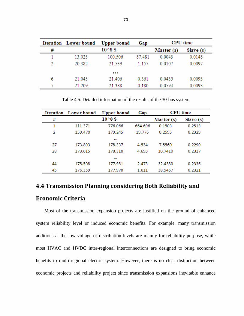
70
Table 4.5. Detailed information of the results of the 30-bus system
4.4 Transmission Planning considering Both Reliability and
Economic Criteria
Most of the transmission expansion projects are justified on the ground of enhanced
system reliability level or induced economic benefits. For example, many transmission
additions at the low voltage or distribution levels are mainly for reliability purpose, while
most HVAC and HVDC inter-regional interconnections are designed to bring economic
benefits to multi-regional electric system. However, there is no clear distinction between
economic projects and reliability project since transmission expansions inevitable enhance
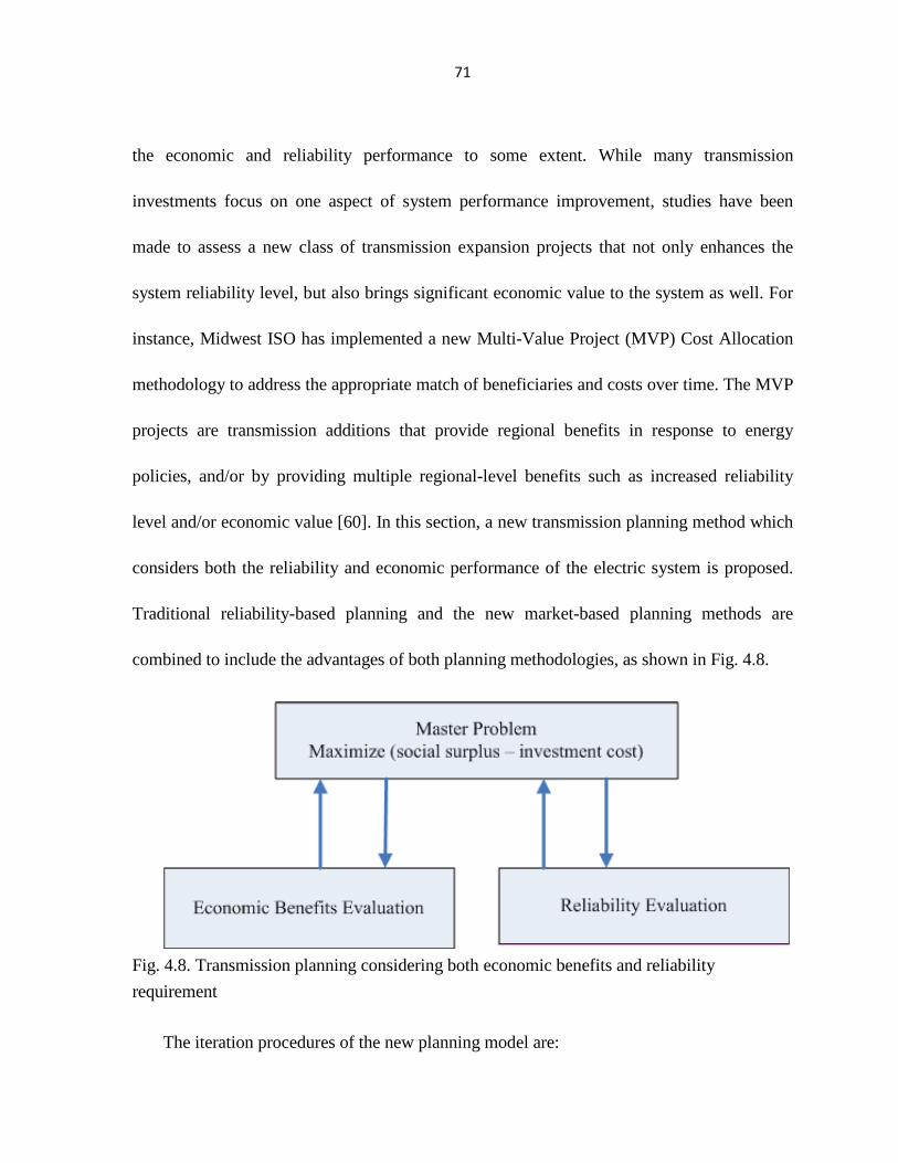
71
the economic and reliability performance to some extent. While many transmission
investments focus on one aspect of system performance improvement, studies have been
made to assess a new class of transmission expansion projects that not only enhances the
system reliability level, but also brings significant economic value to the system as well. For
instance, Midwest ISO has implemented a new Multi-Value Project (MVP) Cost Allocation
methodology to address the appropriate match of beneficiaries and costs over time. The MVP
projects are transmission additions that provide regional benefits in response to energy
policies, and/or by providing multiple regional-level benefits such as increased reliability
level and/or economic value [60]. In this section, a new transmission planning method which
considers both the reliability and economic performance of the electric system is proposed.
Traditional reliability-based planning and the new market-based planning methods are
combined to include the advantages of both planning methodologies, as shown in Fig. 4.8.
Fig. 4.8. Transmission planning considering both economic benefits and reliability
requirement
The iteration procedures of the new planning model are:

72
1. The master problem is solved based on the existing system conditions. A
transmission investment plan is identified.
2. The economic benefits evaluation sub-problem is updated based on the
transmission investment plan proposed by the master problem. Then the slave
problem is solved.
3. A benders optimality check is conducted to check if the current investment plan
is optimal (in terms of economic benefits) or not. If not, an optimality cut will be
added to the master problem.
4. The reliability evaluation sub-problems are also updated based on the
transmission investment plan proposed by the master problem.
5. For each reliability evaluation sub-problem, if the objective function is greater
than 0, the load curtailment is made during a contingency. So a benders
feasibility cut is added to the master problem.
6. If no optimality cut or feasibility cut is added to the master problem, the current
investment plan is optimal and the program stops, otherwise the iteration
continues.
Table 4.6. Comparison of the results of the three planning methods
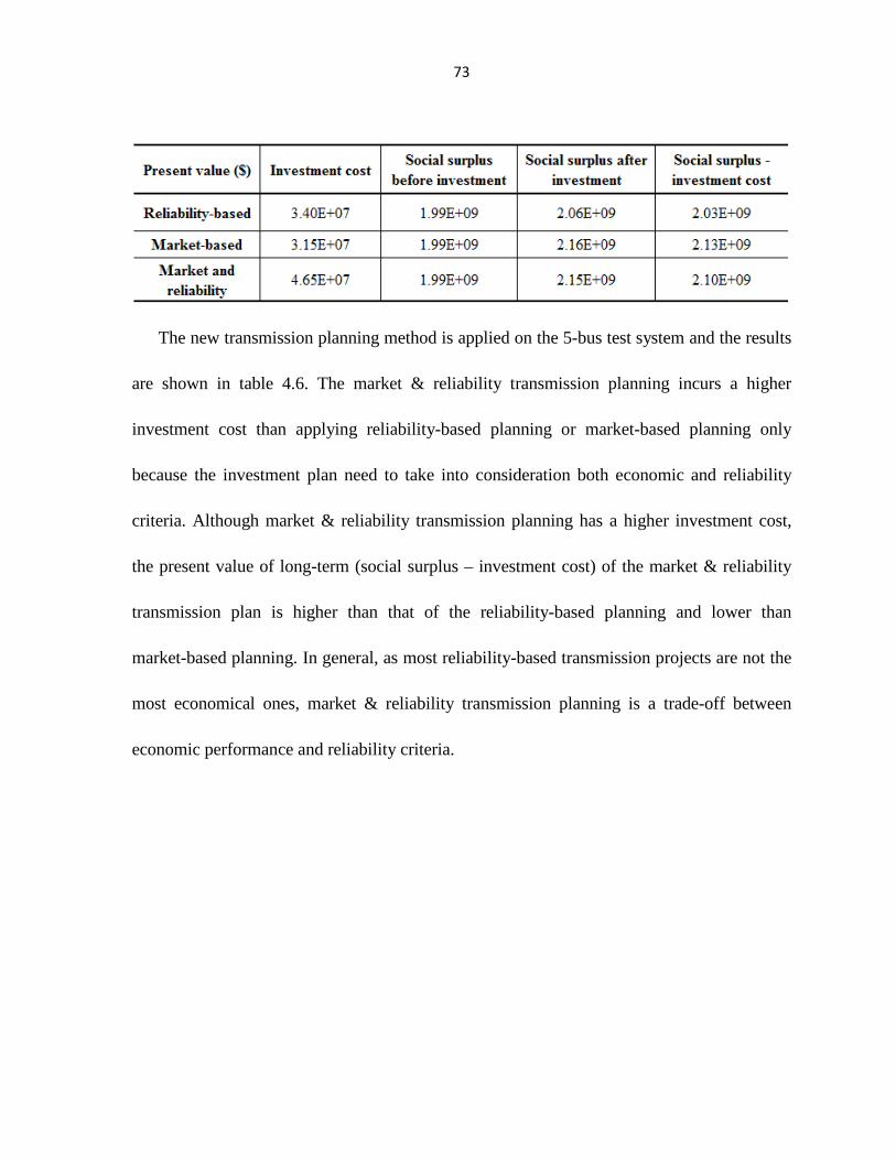
73
The new transmission planning method is applied on the 5-bus test system and the results
are shown in table 4.6. The market & reliability transmission planning incurs a higher
investment cost than applying reliability-based planning or market-based planning only
because the investment plan need to take into consideration both economic and reliability
criteria. Although market & reliability transmission planning has a higher investment cost,
the present value of long-term (social surplus – investment cost) of the market & reliability
transmission plan is higher than that of the reliability-based planning and lower than
market-based planning. In general, as most reliability-based transmission projects are not the
most economical ones, market & reliability transmission planning is a trade-off between
economic performance and reliability criteria.

74
CHAPTER 5 MODELING UNCERTAINTIES
Significant uncertainties occur in the planning model in the deregulated world. Numerous
studies have been made to analyze the effects of uncertainties on the reliability-based
planning model, see [61], [62], and [63]. However, in the deregulated world, uncertainties
have more impacts on transmission expansion planning than on traditional transmission
planning because: 1) Many uncertainties in market-based planning are not considered in
reliability-based planning, e.g. uncertainties in fuel prices. 2) In market-based planning,
uncertainties affect the long-term hourly operations of the electric market. Whereas in the
reliability-based planning, uncertainties’ impacts on the supply-demand balance during the
are peak hours are analyzed. 3) The effects of uncertainties in the market-based model can be
quantified in momentary terms. In the reliability-based planning, however, the effects of
uncertainties are captured by changes in values of reliability indices
In this chapter, the uncertainties that occur in the long-term transmission planning
problem are classified into two categories: random uncertainties (also known as
high-frequency uncertainties), and non-random uncertainties (also known as low-frequency
uncertainties). The two categories of uncertainties are considered in the planning model using
different methods. In order to capture the random uncertainties in the market-based planning
model, Monte Carlo simulation method and Benders decomposition method are combined to
simulate the uncertainties on the operations of the system. The Confidence Interval (CI)
technique is used to check the optimality of the Benders decomposition problem. For

75
non-random variables in the planning model, the robustness testing method is used to identify
one optimal investment plan which works well under all major planning scenarios.
Some studies have been conducted to incorporate uncertainties to the planning models in
the deregulated world, see [1], [7], [64]. Reference [1] uses Monte Carlo simulation
technique to obtain the probability distribution functions of the LMPs during the peak
loading conditions in the planning horizon. Transmission investment decisions are then made
based on several market-based criteria, such as flatness of the price profile, average
congestion cost, average load payment, etc. The minimax regret approach is also used to
minimize the worst-case regret in the planning model [1]. Monte Carlo simulation method is
used to evaluate the system’s operating condition. The decision making problem is separated
from this. Reference [7] also employed Monte Carlo simulation method in the planning
model. In this model, the calculated expected values of LMPs are used in the decision
making problem. However, there are two limitations of the planning model used in [7]: 1) in
the transmission investment problem, there is no iteration mechanism between the master
problem (decision making problem) and slave problem (optimal operation problem) and no
Benders cut in the master problem. So the transmission investment plan generated by the
master problem is solely based on the average LMPs of the original system. The investment
obtained in this way might not be the optimal one as it normal takes several iterations
between the master and the slave problem to get the optimal solution for the whole
optimization problem. For example, tables 4.4 and 4.5 illustrate the gaps between the upper

76
and the lower bounds of the whole optimization problem at different numbers of iterations.
One iteration between master and slave problem might generate big gap which indicate huge
difference between current solution and optimal solution for the whole system. 2) In the
master problem, average LMPs are used to calculate expected production cost. The variance
(risk) of the Monte Carlo simulation results is not considered.
Compared with existing studies on incorporating uncertainties to transmission planning,
the major different features of the model proposed in this chapter are: 1) systematic way to
deals with two categories of uncertainties by combining Monte Carlo simulation with
Benders Decomposition and employing the robustness testing method, 2) ensures optimal
solution for the whole planning problem, 3) variance of the production cost results generated
by the Monte Carlo simulation is captured via building CI, 4) different planning objective.
5.1 Monte Carlo Simulation Method
Monte Carlo method is computational simulation algorithm that generates random trials
to obtain a solution [65]. Monte Carlo method is employed to capture the effects of random
uncertainties in the planning of transmission system. Given the probability density function
of random uncertainties, the deterministic integrated energy system model is then evaluated
iteratively using the values of uncertain parameters which are generated randomly using their
specific probability densities.
The random uncertainties considered in this article are as follows:
i) Uncertainties in fuel prices

77
In the long term planning model, coal price is considered to be constant while natural gas
prices and oil prices are considered to be uncertain. The natural gas prices and oil prices
follow normal distributions and have increasing variances. Essentially, the expected value of
uncertain fuel prices are the same as the forecasted values used in the deterministic case,
however, standard deviations of fuels prices increase over time in order to reflect the
accumulated errors in forecasts.
( ) ( )(1 ( )).
c t c t RC tij s ij s
= + (5.1)
ii) Uncertainties in availability of generation and transmission facilities
We use utij,s(t) and ugi,s(t) in the Monte Carlo simulation to represent transmission line
and generating unit availability. utij,s(t)=0 means that the transmission line between node i
and j has a major outage at time step t while utij,s(t)=1 indicates otherwise; ugi,s(t)=0 means
that generating unit i is not available at time step t while ugi,S(t)=1 indicates it is in service.
utij,s(t) can also be a value between 0 and 1 to indicate that the rating of transmission line is
reduced because of outage or maintenance. At the beginning of each iteration of Monte Carlo
simulation, a random number which follows uniform distribution on [0, 1] is sampled for
each generation unit and transmission line and is compared to the forced outage rate of that
facility. If the random variable is higher than the forced outage rate, then the unit is available
and ugi,s(t) or utij,s(t) is set to be 1. Otherwise it is on outage and ugi,s(t) is set to be 0 if it is a
generating unit or utij,s(t) is set to be 0.6 if it is a transmission line. In the proposed model,
one generator node is split into a pair of generator nodes so that operating constraints and

78
O&M costs can be expressed as the properties of the arc connecting the two nodes. Generator
maximum and minimum output limits are enforced by constraining the energy flow between
the paired generator nodes. In (5.3), when ugi,s(t) is 0, the maximum and minimum
constraints for flow in that arc are both zero, hence the arc flow is zero.
( ) ( ) ( ) ( , ).min . . .max .
e ut t e t e ut t i j Mtij ij s ij s ij ij s
≤ ≤ ∀ ∈ (5.2)
( ) ( ) ( ) ( , ).min . . .max .
e ug t e t e ug t i j Mgij ij s ij s ij ij s
≤ ≤ ∀ ∈ (5.3)
The process to analyze the operation of electric market using Monte Carlo simulation
method is given below:
Step 1) Determine the forecasts of prices of each kind of fuel resources and the load levels.
Step 2) Determine the probability density functions for all of the random uncertainties
mentioned above. For each time step, we need to determine:
• The variances of natural gas and oil prices
• The forced outage rates of generating units and transmission lines
Step 3) Generate a number from the probability density functions of each random variable
and compute the value of its corresponding parameter. For parameter associated with
fuel prices, cij,s(t) is updated for each time t; for parameter about availability of
generating units or transmission lines, the number generated by the standard uniform
distribution is compared with forced outage rate of one unit and then utij,s(t) or ugi,s(t)
is decided.

79
Step 4) Run the slave problem using the inputs and parameters generated in steps 1, 2 and 3
and the decisions made in the master problem.
Step 5) Repeat steps 3 and 4 a large number of times until the results converge.
5.2 Benders Decomposition Iteration Procedures
The combination of Benders decomposition and Monte Carlo simulation method is
employed in the market-based planning approach. Unlike traditional benders decomposition
process, the slave problems are repeated for a large number of times in order to account for
various random uncertainties. Then the program checks the convergence of the results from
slave problems. If the results converge, a statistical test will be carried out to check the null
hypothesis that the population mean is equal to a specified value, otherwise the Monte Carlo
simulation process will increase the number of simulation until the results converge [66].
In each Benders iteration, the master problem generates a set of decisions and an optimal
objective value, which is an upper bound of the real optimal value of the whole planning
problem. Each slave problem can also generate a lower bound of the real optimal value of the
whole planning problem.
In order to check whether the lower bound and the upper bound converge, the confidence
interval of the mean of the whole population of the lower bounds is calculated at each
iteration. Confidence interval is a statistical method to estimate the interval that the true value
of system parameter can lie in. Conference interval method is based on the premise that if the
statistical model is right, large number of observations can help to construct an interval

80
within which the true value of system parameter lies with a specified probability [67].
Although theoretically the confidence interval requires the random variables to be normally
distributed, the confidence interval can be approximated according to central limit theorem.
According to central limit theorem, for n independently and identically distributed random
variables, if the sample size n is large enough, the distribution of sample average 5E (5E =
(x1+ … + xn)/n) is approximately normal with mean µ and variance σ2/n, where µ and σ2 are
mean and variance of the random variable, respectively [67]. In our study, the mean and
variance of the Monte Carlo simulation results are unknown. In this case, the standard
deviation σ is replaced by the standard error s. s can be expressed in the following equation:
12 2( )1
S x xin
= −−
(5.4)
Then given a confidence level α, the confidence interval for the lower bounds calculated
in the Monte Carlo simulation can be expressed as ,cs cs
x xn n
− +
, where c is the 100 α
percentile of the standard normal distribution. For example, when a 95% confidence level is
considered, c is 1.96.
During each iteration, the upper bound is compared with the confidence interval of the
lower bound using (5.5):
(1 )cs
B xupper n
ε− <= − (5.5)
where ε is a very small value. When (5.5) is fulfilled, the upper bound and lower bound are
converged and the optimal solution of the whole transmission planning problem is obtained.

81
Otherwise the iteration continues and an optimality cut is added to the master problem. The
optimality cut is given in (4.16) where Zk is the mean of optimal objective values of all slave
problems.
The employment of confidence interval ensures that not only the mean of the Monte
Carlo simulation results are considered in the planning problem, the variance of the lower
bounds are also used to check the convergence of the whole planning problem. The variance
of the Monte Carlo simulation results (lower bounds) quantifies how sensitive the electric
system is to the random uncertainties considered in the Monte Carlo simulation process. For
example, if the long-term production cost of the system is very sensitive to the oil prices. If
the variation of the results cannot be captured, the transmission plan generated might not be
satisfactory when oil prices are very volatile in the future.

82
Fig. 5.1. The flow chart of Benders decomposition iteration procedures
5.3 Robustness Testing and Multiple Futures
Robustness testing is used to incorporate major non-random uncertainties in the planning
process and identify transmission projects that perform well under most, if not all, Futures.

83
There are two major components in the robustness testing process: defining the Futures and
identifying the attributes that quantify the performance of various investment plans.
A Future is a set of outcomes or realizations of non-random uncertainties [14], for
example: “a Carbon tax of $15 per ton of CO2 emission will be charged.” As different
Futures have different combinations of non-random variables, a transmission investment plan
generated one the basis of one Future might not perform as well in another Future. In other
words, one transmission investment plan might be very sensitive to different Futures. In
order to check the sensitivities of various transmission plans to different Futures, robustness
testing technique is employed in the planning process.
Robustness testing will evaluate the performance of each investment plan under all
Futures. In order to quantify the long-term performance of the investment plan, various
attributes can be identified. Attributes are measures of goodness of a transmission investment
from decision makers’ perspective: production cost, benefit/cost ratio, loss of load
expectation, environmental impact, etc. The values of attributes are decided by investment
plans and Futures. In order to capture various attributes of an investment plan, a production
cost model must be employed to simulate the operations of electric market over the whole
planning horizon. The attributes of each investment plan under the multiple Futures can then
be calculated and compared. The plan that performs consistently well under most Futures
will be chosen.

84
Identifying the best investment plan is a decision making problem as it involves selecting
one investment plan among the optimal investment plans under the multiple Futures. As
mentioned earlier, the attributes of the investment plan reflect the concerns of decision
makers. These attributes might be conflicting in some cases, e.g. lowering production cost vs.
reducing carbon emission. Consequently, the decision making process needs to find a plan
representing reasonable trade-offs among various attributes. Although it is impossible to
thoroughly eliminate the uncertainties in the planning problem, the risk can be managed with
proper techniques. According to [62], risk is “a hazard to which a utility is exposed because
of uncertainty.” Many decision theory techniques have been applied successfully on
managing the risks [62], [63], [68], such as minimax regret approach, maximin approach,
expected value approach, etc. However, these techniques are most useful when only one
attribute is considered and all Futures have the same weight. When multiple attributes are
considered, other methods need to be used to manage the risk. In this section, a scoring
method is used to evaluate the performance of candidate investment plans. The scoring
method is a function of weights on the attributes and each investment plan’s performance
under all Futures. First, the attributes generated by the transmission investments are obtained
from the simulation. Then for each plan and each attribute, the expected value of that
attribute under all the Futures is calculated. For each attribute, the plan that has the highest
expected value of that attribute has a score of 100. For the other plans, their score can be
calculated by dividing their expected values of that attribute by the highest value and then

85
times 100. After the score for each plan on each attributes is obtained, the expected value of
the overall score for each plan can then be calculated. The transmission plan that has the
highest expected overall score is selected as the best one.
The solution steps for the proposed transmission planning problem are given as follows:
Step 1) Identify major non-random uncertainties, such as carbon tax, carbon cap-and-trade,
high wind penetration level, and new generation technologies. Then multiple futures
are generated, each representing a certain set of non-random uncertainties. Futures
can have different weight to represent their probabilities of occurrence or how
important the decision makers think they are.
Step 2) Monte Carlo simulation generates a set of scenarios assuming uncertainties of fuel
prices, future load growth, availability of generation and transmission units, and
capacity factor of wind turbines. Then the market-based transmission planning
problem is solved under these random uncertainties and under each Future.
Step 3) Under each Future, the electric system is updated based on the assumptions made in
step one. Then the transmission expansion planning model is executed and one
investment plan is generated.
Step 4) After the preliminary transmission plans under each Future are identified, each
preliminary transmission plan must be analyzed under the other Futures to test its
robustness. Several attributes of an investment plan are identified, such as social
surplus, greenhouse gas emissions, reserve margin, and reliability of electric system.

86
A long-term production cost model is used to calculate the values of each attributes
under each Future for each investment plan. Then the attributes under multiple
Futures are obtained and scores are calculated. The plan with the highest overall
score is selected.
5.4 Numerical Example
The planning model is applied on the same 5-bus system as shown in Fig. 4.6. Four
Futures are considered in the robustness testing part.
Future 1: base case.
Future 2: a 20% wind penetration level is enforced so 3 wind farms will be built in node 1, 3
and 5 with capacity 250 MW, 200 MW and 125 MW, respectively.
Future 3: a 20% wind penetration level is enforced and a 15 $/tCO2 carbon tax will be
charged since year 1.
Future 4: a 15 $/tCO2 carbon tax will be charged since year 1.
Table 5.1. The weights of the four Futures
The weights of the four Futures are considered in this study. The weights represent the
possibilities of occurrences of these Futures.
Table 5.2. Four investment plans
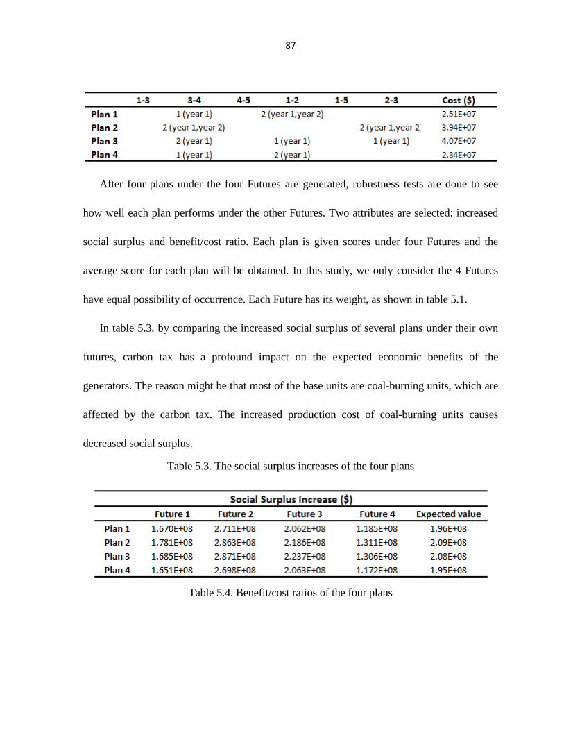
87
After four plans under the four Futures are generated, robustness tests are done to see
how well each plan performs under the other Futures. Two attributes are selected: increased
social surplus and benefit/cost ratio. Each plan is given scores under four Futures and the
average score for each plan will be obtained. In this study, we only consider the 4 Futures
have equal possibility of occurrence. Each Future has its weight, as shown in table 5.1.
In table 5.3, by comparing the increased social surplus of several plans under their own
futures, carbon tax has a profound impact on the expected economic benefits of the
generators. The reason might be that most of the base units are coal-burning units, which are
affected by the carbon tax. The increased production cost of coal-burning units causes
decreased social surplus.
Table 5.3. The social surplus increases of the four plans
Table 5.4. Benefit/cost ratios of the four plans

88
Table 5.5. Final scores of the four plans
According to the results given in table 5.5, plan 4 has the highest overall score (95.96), so
it is selected. Although plan 2 and 3 outperform plan 4 in terms of the first attribute, plan 4
has a higher benefit/cost ratio than the other plans. In table 5.5, the weights of the two
attributes are considered. The weight on the attribute reflects how important the decision
maker think it is.
This study only considers two attributes: social surplus increase and benefit/cost ratio.
However, the robustness testing technique used in this study can consider more attributes if
needed. As long as these attributes are properly defined and their weights are fixed, the risks
associated with non-random uncertainties can be managed and one optimal investment plan
can be selected.

89
CHAPTER 6 TRANSMISSION PLANNING
CONSIDERING LARGE-SCALE INTEGRATION OF
RENEWABLE ENERGY
6.1 Introduction
In the last decade, there has been significant growth in US wind capacity, partly because of
advances in wind generation technology, government subsidies, and other policy incentives.
By October 2010, 31 states had a Renewable Portfolio Standard (RPS) and an additional 7
states had goals for renewable energy deployment, and so it is apparent that wind capacity
will continue to increase in the coming years.
The economic impact of such a highly variable energy source needs to be assessed as wind
power penetration level keeps increasing. Compared to other conventional power sources,
wind power has many unique characteristics which have significant impacts on the operation
and planning of electric system. First, the majority of the wind resource is located remote
from the major load centers. For example, in the US most of the wind-rich areas are in
Mid-west and Texas which are far away from major urban and industrial centers—where
demand for energy is greatest. Long transmission lines with high capacities would be
necessary to transport the most economically attractive wind power from where it is
generated to where it is consumed. Second, as wind resource in variable in nature, there will
be increased volatility in LMPs in the market. Third, as wind energy is less dispatchable than
conventional generators, when the wind penetration level is high, it is more difficult for

90
system operators to balance the market. Currently, system operators commit generating units
based on forecasts of load and wind generation, and then dispatch the available units against
the actual quantities. While there are mature models and enough historical data to accurately
forecast the load level in the next day, hour or minute, there are still high forecasting errors in
wind generation. There are energy imbalances in the market as the result of forecasting errors.
Fourth, wind energy cannot be used as system reserve, so as wind penetration level increases,
more reserve is required. With the increase of wind penetration level, there are less energy
generated by conventional generators in the market. Wind farms cannot be used as a source
of reserve, so more reserves are required to secure the reliable operation of the electric
system and more regulations costs are incurred. Finally, as wind energy is negatively
correlated with the demand, large-scale energy storage capabilities are needed. During the
peak hours when the demand and electricity price are high, wind generation is generally low;
during the off-peak hours when there are less demand and lower price, wind farms have
maximal generation. So it makes sense to invest energy storage facilities to store the low-cost
wind energy during the night and sell it to the market during the peak hours when the price is
high.
As the current transmission is not designed to transport the large amount of wind power, a
lot of congestions occur in the system. With the increase of wind penetration, more and more
wind power is curtailed out of the market for transmission bottlenecks and minimum
generation events. Congestion will cause price differences among the nodes connected by

91
that transmission line, which indicate that the market is not operating efficiently as electric
power from the lower-price end cannot be freely transferred to the high-price end.
Consumers will pay more for electricity as LSEs cannot access the low-cost supplies. The
result of the congestion is lower market efficiency and less competition. As stated in FERC
order 2000, two of the minimal functions that an RTO must perform are managing the
congestion and planning transmission system expansion [69]. So from ISO/RTO’s point of
view, efforts must be made to expand the transmission system in order to alleviate the
congestions caused by excess amount of wind power. By adding more transmission to the
system properly, less expensive resources that had previously been curtailed are given an
opportunity to be used by the system.
The economic impacts of large-scale wind power on the operation and planning of bulk
electric transmission are investigated and illustrated in this chapter. The market-based
transmission expansion planning method is modified in order to capture the unique features
of wind power and storage system. The market-based transmission planning model can
justify transmission additions at a regional level which facilitates the efficient utilization of
large-scale wind power.
Most planning optimization tools optimize generation expansion plans under an assumed
transmission expansion plan, or they optimize transmission expansion plans under an
assumed generation expansion plan. In practice, engineers typically find optimal transmission
expansion plans for various generation expansion futures, often iterating between generation

92
planning and transmission planning results, settling on those transmission expansion plans
which are needed under most or all of the generation expansion futures [60]. Inadequately
accounting for the interdependency between the two planning processes may result in
suboptimal investment decisions and lost economic benefits. In this chapter, the interactions
between large-scale wind integration and transmission system planning are analyzed, and a
new computational procedure of system expansion planning that coordinates generation and
transmission investment is proposed.
6.2 Wind Formulation
Wind farms’ generation outputs are highly volatile. Many attempts have been made to
use various statistical methods to capture the wind power output characteristics, such as using
wind generation probability density function (pdf) [70], auto-regressive moving average
(ARMA) model [71], or multivariate statistical model [72]. For wind and storage related
production cost simulation, a purely “Monte Carlo” sampling using wind generation pdf
cannot capture the inter-temporal system dependencies. ARMA is accurate for short-term
wind generation forecast. However, it is not suitable for long-term simulation as its accuracy
tends to degrade with increasing lead time. The multivariate sequential time-series method
has been used with success to model the wind power inter-temporal variations over long
period of time [73]. In this study, a nominal 1-MW multivariate wind power hourly
production time series is used for each wind farm. The 1-MW wind power time series
contains the hourly maximum power output information for a wind farm with 1 MW capacity
93
in a specific geographic area. As 1-MW wind power time series is independent of the wind
farm capacity, it can be used in the planning model to determine the maximum power output
for each hour.
6.3 Generation Expansion Planning Model
With the focus on promoting the use of renewable energy, the efficient and cost-effective
integration of wind energy to the grid is becoming increasingly important. As the decision
makers for the wind integration are generation companies, the generation expansion planning
model is formulated from their perspective. The proposed wind generation expansion
planning (GEP) model optimizes the large-scale wind power integration by maximizing the
expected profits of the wind farms minus the investment costs.
As shown in Fig. 1, the wind generation expansion planning model is decomposed into a
master problem, which identifies generation investment decisions, and two slave problems,
which simulate the hourly operations of the electric system over the whole planning horizon.
The slave problems are comprised of one unit commitment (UC) problem and one economic
dispatch (ED) problem. In order to fully capture the impacts of large-scale wind integrations,
the co-optimization of the energy market subject to transmission constraints and the ancillary
service market subject to resource constraints is implemented. As the result of the
co-optimization, the reserve price will reflect the marginal cost of the services as well as any
lost opportunity cost incurred by having to back up rather than bidding in the energy market.

94
The overall planning problem is solved by iterating between the master and the slave
problems. In each iteration, the master problem generates a set of investment decisions and
passes them to the slave problems. The slave problems simulate the operations of the market
using the solution obtained in the master problem. Then the Benders optimality rule is used
to check whether the optimal solution is achieved. If not, an optimality cut will be added to
the master problem, and generation companies’ total profits can be calculated. Then the next
iteration gets started. Otherwise the final investment plan is obtained.

95
Fig. 6.1. Wind generation expansion planning model
In the production cost simulation model, the hourly operations in a day-ahead energy and
ancillary service markets are considered. In the energy market, each generator submits

96
energy bids to the independent system operator (ISO) according to their marginal production
costs. No strategic bidding is considered in this article.
In the ancillary service market, each eligible generator submits hourly bids for the next
day for ancillary services, i.e. operating reserve [74]. Operating reserve is used to ensure the
reliable and secure operations of the system under normal and emergency conditions.
Operating reserve can be divided into two categories: regulating reserve and contingency
reserve. The former is provided by generators’ automatic generation control (AGC) devices
to compensate the minute to minute frequency deviations in the network, while the latter is
used to respond to system contingencies, such as losses of generating units or transmission
lines. There are two types of contingency reserves, spinning reserve and non-spinning reserve.
Only those generators that are running and can provide fast response (fully available within
10 minutes) to system imbalance can bid for the spinning reserve. Non-spinning reserve is
off-line generation capacity that can be ramped to capacity and synchronized to the grid
within 10 minutes. In order to assure that the highest quality service is procured if
economically appropriate, higher quality reserve (spinning reserve) can substitute for low
quality reserve (non-spinning reserve).
After the bids in both the energy and ancillary service markets are received, ISO
dispatches generation resources based on bid-clearing methodology. In the day-ahead market,
the co-optimization of the energy market subject to transmission constraints and the ancillary
service market subject to resource constraints is implemented. In this way, both markets are

97
cleared simultaneously. The clearing of the energy and ancillary service markets is a
two-stage procedure. First, a unit commitment (UC) problem is solved to commit the
generating resources. Based on the unit commitment schedule, an economic dispatch (ED)
problem is then solved to dispatch the generators in the most economical way.
6.3.1. Unit Commitment Problem Formulation
The unit commitment problem is formulated as a mixed-integer optimization problem.
The objective function is the minimization of {the total energy and ancillary service biddings
+ start-up costs + shut-down costs + loss of load penalties}. As the result of the
co-optimization of the energy and ancillary services markets, the reserve price will reflect the
marginal cost of the services as well as any lost opportunity cost incurred by having to back
up rather than bidding in the energy market. Regulating reserve is not considered in this
formulation as the time step considered here is one hour, while regulating reserve are
generally used in the 1 minute to 10 minute time frame in order to provide fast response to
load variations. The results of the UC problem are the operating schedules for all the
generators at each time step.
( , ) ( , ) ( ) ( ) ( , ) ( , )( , ) ( , )
( , ) ( , ) ( ) ( )
( , ) ( ) ( )
Ce l t e l t lol t r t Cs s t f s tij ij j ij iji j M l L j N i j M s Sij ij
MinCn ns t g ns t Su Ux t SdUy tij ij ij ij ijt T
i j M ns NS ij Mg ij Mgij
+ +∑ ∑ ∑ ∑ ∑∈ ∈ ∈ ∈ ∈
∑+ + +∑ ∑ ∑ ∑∈
∈ ∈ ∈ ∈
(6.1)
At each node, the sum of flow injections minus the sum of flow extractions is the demand
at that node.

98
( , ) ( , ) ( ) ( ), , ( ) , ( ) e l t e l t r t d t j N ij M jk Mij ij jk j j ti l L k l Lij jk
η − + = ∀ ∈ ∀ ∈ ∀ ∈∑ ∑ ∑ ∑∀ ∈ ∀ ∈
(6.2)
In order to capture the limits on generator ij ’s output at each time step, two kinds of
constraints are considered: the constraints on each segment of generator ij ’s bidding curve
and the constraints on generator ij ’s total generation level. If generator ij is online at time t
(Uij=0), then its energy bidding segment l must satisfy the upper and lower flow limits,
otherwise it is zero. In order to make sure that the commitment schedule is considered in the
equation, the UC decision variable is included in the upper and lower bounds.
( ) ( ) ( , ) ( ) ( ), ( )e l U t e l t e l U t ij Mgij ijij ij ij≤ ≤ ∀ ∈ (6.3)
In the UC problem, the transmission system is simulated using a transportation model,
which considers the flow limits only.
( ) ( , ) ( ), ( )e l e l t e l ij Mtij ijij≤ ≤ ∀ ∈ (6.4)
For generator ij , the sum of {energy + spinning reserve + non-spinning reserve} must be
less than its thermal limit. If a unit is on-line, it can submit energy, spinning, and
non-spinning reserves offers. If it is off-line, it can only bid non-spinning reserve. In both
cases, the sum of three biddings needs to be constrained by the generator’s maximum
capacity.
( , ) ( , ) ( , ) ( ), ( , )e l t f s t g ns t e l i j Mgij ij ij ijl L s S ns NS l Lij ij ij ij
+ + ≤ ∀ ∈∑ ∑ ∑ ∑∈ ∈ ∈ ∈
(6.5)
99
The spinning reserve provided by generator ij must follow its capacity constraint. When
the unit is off-line, it cannot bid any spinning reserve. Equation (6.5) and (6.6) makes sure
that spinning reserve can substitute non-spinning reserve when the unit is synchronized to the
grid.
( , ) ( ) ( )f s t U t e lij ijijs S l Lij ij
≤∑ ∑∈ ∈
(6.6)
In order to ensure the reliable operation of the energy system, sufficient operating reserve
needs to be provided at each time step. Spinning and non-spinning reserves are considered in
this article, with the possibility of including more reserve types in the future. Operating
reserve is defined as:
OR = max{OR1,OR2} + 100% of non-firm imports
where OR1 is 5% of hydro generation + 7% of generation provided by other conventional
generators (excluding intermittent generation resources) + x% of wind power output (x is a
number higher than 7); OR2 is the MW loss of generation due to the outage of the largest
generating unit at each hour. Spinning reserve needs to be at least 50% of the operating
reserve requirement. The reasons for the fact that hydro generation requires less reserve and
wind generation requires more reserve than traditional generators are that non-hydro
generation has additional risks related to fuel scheduling and wind generation has much
higher variations in its output. This definition of operating reserve is in line with California
ISO’s operation reserve requirement and is similar with that of many other ISO/RTOs [75].

100
Spinning reserve requirement:
1( , )
2( , )f s t ORij
i j Mg s Sij
≥∑ ∑∈ ∈
(6.7)
Non-spinning reserve requirement:
1( , )
2( , )g ns t ORij
i j Mg ns NSij
≥∑ ∑∈ ∈
(6.8)
Constraint (6.9) shows that at each time step, the maximum generation output is
constrained by the wind maximum generation time series forecast.
( , ) ( ) ( ), ( )e l t C t wo t ij Mwij ij ijl Lij
≤ ∀ ∈∑∈
(6.9)
A generator’s start-up and shut-down costs are considered in the objective function. Ux
and Uy are binary variables indicating whether unit ij is switched on or shut down at time t or
not, respectively.
( ) ( 1) ( ) ( ), ( )U t U t Ux t Uy t ij Mg
ij ij ij ij− − = − ∀ ∈
(6.10)
A generating unit has limited ability to vary its generation output from one time step to
the next.
Up-ramp constraints:
( , ) ( , 1) ( )e l t e l t ru ij Mgij ij ijl Lij l Lij
− − ≤ ∀ ∈∑ ∑∈ ∈
(6.11)
Down-ramp constraints:
( , 1) ( , ) ( )e l t e l t rd ij Mgij ij ijl Lij l Lij
− − ≤ ∀ ∈∑ ∑∈ ∈ (6.12)

101
The configurations of CAES are modeled as three parts: the compressor, the gas
turbine/generator, and the air reservoir. At the end of time step t, the energy stored at the air
reservoir is decided by the storage level at time step (t-1), energy stored at time step t, and
storage’s power output at time step t.
( ) ( 1) ( ) ( , ), e t e t e t e l t i Nsijii ii ki kil Lij
iiη η= − + − ∀ ∈∑
∈ (6.13)
Storage system can provide not only electric power, but also spinning and non-spinning
reserves. In (6.5), the sum of {energy + spinning reserve + non-spinning reserve} is
constrained by that generator’s maximum output. For storage system, the maximum amount
of {energy + spinning reserve + non-spinning reserve} at time step t should also be limited
by the storage level at time step (t-1).
( , ) ( , ) ( , ) ( 1),e l t e s t e ns t e t i Nsij ij ij iil L s S ns NSij ij ij
iiη+ + ≤ − ∀ ∈∑ ∑ ∑
∈ ∈ ∈ (6.14)
6.3.2. Economic Dispatch Problem Formulation
Based on the commitment schedule generated by the UC problem, the ED problem
dispatches the generating units in the minimal cost way and obtains LMPs at each node for
energy and market clearing prices (MCP) for ancillary service. Unlike the UC problem, the
ED problem considers the transmission network using the DC-OPF formulation.
( , ) ( , ) ( ) ( ) ( , ) ( , )( , ) ( , )
( , ) ( , )
( , )
Ce l t e l t lol t r t Cs s t f s tij ij j ij iji j M l L j N i j M s Sij ij
MinCn ns t g ns tij ijt T
i j M ns NSij
+ +∑ ∑ ∑ ∑ ∑∈ ∈ ∈ ∈ ∈
∑+ ∑ ∑∈
∈ ∈
(6.15)

102
The ED problem is similar with the UC problem in most parts except that uij is a
parameter, not a variable. The start-up and shut-down costs are fixed after the unit
commitment schedule is decided so they are not considered in ED problem’s objective
function. As there is no integer variable in the optimization problem, the ED problem is a
linear optimization problem.
( , ) ( , ) ( ) ( ), , ( ) , ( ) e l t e l t r t d t j N ij M jk Mij ij jk j j ti l L k l Lij jk
η − + = ∀ ∈ ∀ ∈ ∀ ∈∑ ∑ ∑ ∑∀ ∈ ∀ ∈
(6.16)
( ) ( ) ( , ) ( ) ( ), ( )e l u t e l t e l u t ij Mgij ijij ij ij≤ ≤ ∀ ∈ (6.17)
( ) ( , ) ( ), ( )e l e l t e l ij Mtij ijij≤ ≤ ∀ ∈ (6.18)
( , ) ( , ) ( , ) ( ), ( , )e l t f s t g ns t e l i j Mgij ij ij ijl L s S ns NS l Lij ij ij ij
+ + ≤ ∀ ∈∑ ∑ ∑ ∑∈ ∈ ∈ ∈
(6.19)
1( , )
2( , )f s t ORij
i j Mg s Sij
≥∑ ∑∈ ∈
(6.20)
1( , )
2( , )g ns t ORij
i j Mg ns NSij
≥∑ ∑∈ ∈
(6.21)
( , ) ( ) ( )f s t u t e lij ijijs S l Lij ij
≤∑ ∑∈ ∈
(6.22)
( , ) ( ) ( ), ( )e l t C t wo t ij Mwij ij ijl Lij
≤ ∀ ∈∑∈
(6.23)
( ) ( 1) ( ) ( , ),e t e t e t e l t i Nsijii ii ki kil Lij
iiη η= − + − ∀ ∈∑
∈ (6.24)
( , ) ( , ) ( , ) ( 1),e l t e s t e ns t e t i Nsij ij ij iil L s S ns NSij ij ij
iiη+ + ≤ − ∀ ∈∑ ∑ ∑
∈ ∈ ∈ (6.25)
103
With some modifications, DC-OPF algorithm is employed in the ED problem. Equation
(2.12) and (2.13) represent the Kirchhoff’s voltage law.
( , ) ( ( ) ( )) 0, ( )e l t b t t ij Mtij ij i jl Lij
θ θ− − = ∀ ∈∑∈
(6.26)
, i Nti
π θ π− ≤ ≤ ∀ ∈ (6.27)
When ED problem is solved, the generation dispatch schedule for each generation unit is
decide. As the byproducts of the optimization problem, the LMP in each node and MCP for
spinning and non-spinning reserves can be obtained.
6.3.3. GEP Master Problem Formulation
The master problem minimizes the investment cost and the present value of wind
generator profits. Constraint (6.30) is the benders optimality constraint which forces the
master problem to generate the optimal investment plan for the whole planning problem.
Constraint (6.30) refers to the renewable penetration target which requires certain wind
penetration levels to be fulfilled each year. Constraints (6.31), (6.32), (6.33) update the total
number of wind farms built each year and the constraints on the number of investment each
year and the total number of wind farm that can be built.
(1 ) ( )( , )
tMin r I m t Zij ijt T i j Mg
− ∗+ +∑ ∑∈ ∈
(6.28)
Subject to:
0Z∗ ≤ (6.29)

104
(1 ) ( , ) ( , ) (1 ) ( ) ( , )( ) ( )
( ) ( )( )( )
t k t k kZ r Ce l t e l t r t e l tij ij j ijt T ij Mwl L t T ij Mwl Lij ij
k kwc t wo t n nj ij ij ijt T ij Mw
λ
λ
∗ − −≥ + − +∑ ∑ ∑ ∑ ∑ ∑∈ ∈ ∈ ∈ ∈ ∈
− −∑ ∑∈ ∈
(6.30)
( ) ( ) 0( )
C t w D w tij ij avg ijij Mw
σ δ− ≥∑∈
(6.31)
( ) ( 1) ( ), ( )n t n t m t a ij Mwij ij ij
= − + − ∀ ∈ (6.32)
0 ( ) , ( )m t m ij Mwijij≤ ≤ ∀ ∈ (6.33)
0 ( ) , ( )n t n ij Mwijij≤ ≤ ∀ ∈ (6.34)
6.4 Transmission Expansion Planning Model
In this section, a market-based transmission planning model in a wholesale electricity
market with double-sided auctions is formulated. The market-based transmission is justified
based on the trade-off between investment costs and an increase in economic value incurred
by network expansions. Effective transmission expansions will promote market efficiency,
lower energy delivery cost, enhance system reliability, and mitigate significant market power.
In order to quantify the economic benefits brought by transmission investment, the value of
transmission investments in the energy market and ancillary service market are considered.
According to economic theories, social surplus is a good indicator of how well a market is
working. Thus, social surplus is used to quantify the economic benefits that network
expansions bring to the energy market. Transmission additions can resolve transmission
bottlenecks so local reserve needs can be fulfilled by remote low-cost generators. As local

105
reserve requirement is now satisfied by a larger fleet of generators, the total ancillary service
cost is reduced. Thus, reduction in ancillary service cost is used to quantify the economic
benefits that network expansions bring to the ancillary service market. In the objective
function, (energy cost + ancillary service cost + investment cost) is minimized to ensure that
transmission investments can bring at least as much economic benefits as costs. The master
problem makes transmission investment decisions and the slave problem is the same as that
of the generation expansion planning problem.
Fig. 6.2. Transmission expansion planning model
In this paper, we assume an ISO will conduct the market-based transmission planning
study for the whole system in order to find the profitable investment opportunities for
companies or individual investors that are interested. In the objective function, the total
present value of system production costs and investment cost is minimized. Constraint (6.30)
is the benders optimality cut that is added to the master problem at each iteration.

106
(1 ) ( )( , )
tMin r I m t Zij ijt T i j Mg
− ∗+ +∑ ∑∈ ∈
(6.28)
Subject to:
0Z∗ ≥ (6.29)
( )( ( ) ( ))( ) '
k k kZ Z t n t n tij ij ij
t T ij Mnδ∗ ≥ −∑ ∑
∈ ∈− (6.30)
( ) ( 1) ( ), ( )n t n t m t a ij Mwij ij ij
= − + − ∀ ∈ (6.31)
0 ( ) , ( )m t m ij Mwijij≤ ≤ ∀ ∈ (6.32)
0 ( ) , ( )n t n ij Mwijij≤ ≤ ∀ ∈ (6.33)
6.5 Coordinating GEP and TEP
As the planning and decision making for wind integration and transmission investment
are separated, the two processes are usually considered as two independent problems.
However, both wind and transmission investments will have profound impacts on each other
as they will affect the topology of the system and the operation of the market. In order to
capture the interactions between large-scale wind integration and transmission planning, a
coordinated system expansion planning was formulated. First, the generation planning is
conducted. Then the resulted generation investment plan is transferred to the transmission
planning model. The TEP model will update the system information based on the generation

107
investment plan and generate a transmission investment plan which is then passed to the GEP
model. This iteration continues until there is enough coordination between the two processes.
Fig. 6.3. Coordinate the two planning processes
6.6 Numerical Example

108
Fig. 6.4. IEEE 24-bus reliability test system
The proposed methodology is applied on a modified IEEE 24-bus reliability test system
(RTS) [76]. The planning horizon is 10 years. Some modifications to the original system
were made. The load levels increase by 5% per year while the generators’ bidding prices
increase by 4% per year. The capacities of generators 16, 18, 21, 22 and 23 are increased by
50% at year five.
A 20% wind penetration level is required by the 10th year. There are four candidate wind
sites and the capacity factors of the wind farms in these sites are shown in table 6.1.
Table 6.1 Capacity factors for candidate wind sites

109
In order to identify the candidate lines, a method named Copper Sheet method was used.
“Copper Sheet” analysis illustrates the increase in energy flows in various transmission paths
if the transmission constraints were removed. Firstly, the system average flows over the
whole planning horizon were calculated. Then, assuming that the system did not have any
transmission line flow limits, the system average flows were calculated. By comparing the
results of the two cases, we could identify some candidate lines to invest. The huge changes
in averages flows means that the congestions in the system had a significant impact on the
lines. So these lines should be considered as candidate lines. In this process, nine candidate
lines are selected and shown in bold in table 1.
Table 6.2 Results from the Copper sheet method

110
As the Copper Sheet method can only show the changes of flows in existing lines,
additional analysis needs to be made to identify candidate lines between buses that were not
connected currently. If the existing transmission system is not well designed, the topology of
the network might be the major reason for the transmission bottlenecks. In this work, a long
term production cost problem is applied to the test system. As the by-product of the production
cost problem, the LMP of each load at each hour can be obtained. The existence of congestions
in transmission lines will cause the differences in LMPs of the buses connected by the lines.
Table 6.3 Average LMP of each bus
Table 6.2 shows the average LMP of each bus over the planning horizon. As shown in
table 6.2, generally the buses in the upper region, where there are significant amount of wind
power and plenty of low-cost coal plants, have lower LMPs; while buses in the lower region,
where the transmission system has huge congestions, have higher LMPs. It makes senses to
add candidate lines to connect the two regions in order to transfer the low cost energy to the
high energy price area. Two candidate lines (EL11EL21 and EL12EL22) are identified at the
end of this process.

111
Fig. 6.5. GEP results from the original system
After all of the candidate transmission lines are identified, the GEP and TEP are conducted
and coordinated. In this study, 5 iterations of GEP and TEP are considered. Fig. 6.5 shows the
generation expansion results when applying the GEP model to the original system. As shown
in fig. 6.5, most of the new wind units are built in sites near the load center although they have
lower capacity factors compared with that of the sites far away from the load center. This might
due to the high congestions in the transmission lines linking wind rich areas with the load
center. When there are congestions, the wind energy from remote wind rich areas cannot be
transferred to the demand center. Consequently, although bus 21 and bus 22 have high capacity
factors, most wind units are built on bus 11.
Table 6.4 TEP results from the original system
0
2
4
6
8
10
12
1 2 3 4 5 6 7 8 9 10
Ca
pa
city
(1
00
MW
)
Year
Bus 22
Bus 21
Bus 17
Bus 11

112
Table 6.4 shows the results of the TEP. Transmission lines are built to connect the upper
region, where low-cost generators are located, to the lower region, where the demand is high.
Fig. 6.6. GEP results from the fifth iteration
Fig. 6.6 shows the GEP results from the fifth iteration between generation planning and
transmission planning. As previous transmission planning processes have already identified
new transmission lines that can relieve the congestions between the two regions, more
capacities are built in the upper region. If it were not for the coordination between GEP and
TEP, most of the wind units would have been built in sites that have lower capacity factors.
Table 6.5 TEP results from the fifth iteration
0
1
2
3
4
5
6
7
8
9
10
1 2 3 4 5 6 7 8 9 10
Ca
pa
city
(1
00
MW
)
Year
Bus 22
Bus 21
Bus 17
Bus 11

113
Comparing table 6.4 and table 6.5, we can notice the differences between conducting
TEP one the original system and coordinating TEP with GEP.
Table 6.6 Results from the two cases
The simulation results obtained from this case study illustrate the impacts of
coordinating the GEP and TEP processes on both the generation system and the transmission
system. As shown in table 6.6, coordinating GEP and TEP yields a higher system social
surplus. The social surplus of the original system is $1.01E+09, so the social surplus increase
incurred by the GEP and TEP coordination is about 3.8 times as much as the social surplus
increase caused by conducting GEP and TEP separately. The fundamental advantage of
coordinating GEP and TEP is that this planning method can find the optimal generation and
transmission investment plans and bring maximum economic benefits to the system. When
GEP and TEP are conducted separately, wind rich areas that are remote from load center are

114
not selected as the result of transmission congestions, so more wind capacity needs to be
invested to satisfy the wind penetration target as wind sites near the load center generally has
lower capacity factor. When GEP and TEP are coordinated, more transmission lines are
invested to transfer the wind energy from remote wind sites to load center. There is a much
higher benefit/cost ratio in the GEP/TEP coordination case compared to conducting GEP and
TEP separately (3.19 v.s. 0.81). When the interaction between GEP and TEP is considered,
more accurate information about the current and future generation system can be obtained.
So the transmission planning process can evaluate the system conditions thoroughly and
generates a transmission investment plan that can maximize the (system social surplus –
transmission investment costs).
More studies are needed to simulate how the current electricity industry coordinates the
TEP and GEP and to come up with the better mechanism to stop the interaction between the
two processes. Moreover, further studies are required to explore possible market rules or
planning methodology than can promote the efficient system capacity expansion planning
and generate more economic benefits from the generation and transmission investment.

115
CHAPTER 7 EVALUATING ENERGY STORAGE
SYSTEM AS AN ALTERNATIVE TO TRANSMISSION
EXPANSIONS
7.1 Introduction
With the focus on promoting the use of renewable energy, the efficient and cost-effective
integration of wind energy to the grid is becoming increasingly important. While
transmission system investment can solve the problem associated with transferring the large
amount of wind energy in the grid in the long run, significant lead-time and investment
hampers the transmission system expansion. The overall system capacity expansion plan
should consider the generation and demand-side alternatives to transmission constructions. In
the short term, in order to relieve the bottlenecks in the system and promote the efficient
operation of the market, other investments can be considered to maximize the use of the
electric system. Recently, a number of studies have been carried out to evaluate the
possibility of using various kinds of Energy Storage Systems (ESS) to offset the wind
generation variation [77], [78], [79], [80]. Energy storage systems can be used to purchase
and store energy when the price is low and sell it to the market when energy price is high.
Besides peak shifting and load leveling, energy storage can also be used to provide
high-value ancillary services, enhance the stability of electric system, and serve as a
substitute for transmission line investment. Moreover, as most energy storage systems can
provide fast response, they are the ideal options to counterbalance wind output variability.
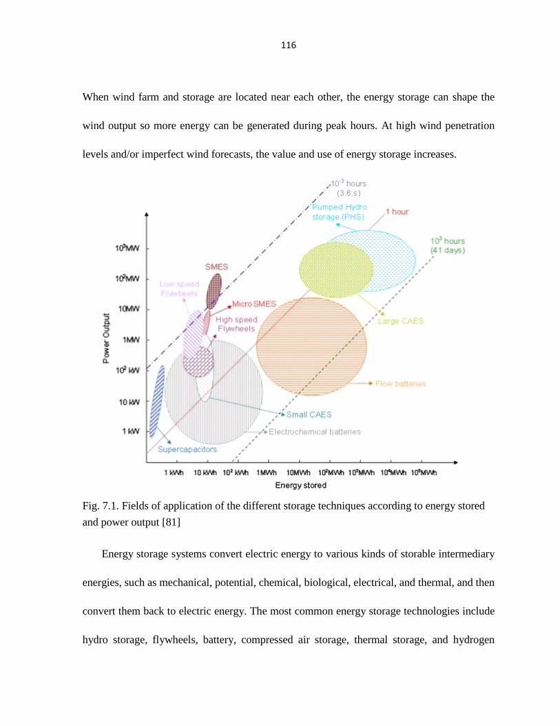
116
When wind farm and storage are located near each other, the energy storage can shape the
wind output so more energy can be generated during peak hours. At high wind penetration
levels and/or imperfect wind forecasts, the value and use of energy storage increases.
Fig. 7.1. Fields of application of the different storage techniques according to energy stored
and power output [81]
Energy storage systems convert electric energy to various kinds of storable intermediary
energies, such as mechanical, potential, chemical, biological, electrical, and thermal, and then
convert them back to electric energy. The most common energy storage technologies include
hydro storage, flywheels, battery, compressed air storage, thermal storage, and hydrogen

117
storage. A comparison of fields of application of different storage technologies is shown in
Fig. 7.1. An extensive comparison of energy storage systems is shown in [82]. One of the
major obstacles of the wide adoption of energy storage systems is their economic
justification. Converting electric energy to another form and converting it back involves high
energy losses and costs. Pumped hydro and compressed air energy storage (CAES) are bulk
energy storage options. Pumped hydro storage is the most widespread energy storage system
today with about 90 GW of installed capacity which accounts for around 3% of global
generation capacity. However, pumped hydro is very site-specific and involves high capital
cost. It also has adverse effects on the environment [83]. CAES is a modification of gas
turbine (GT) technology, where off-peak (low-cost) electrical power is used to compress air
into an underground air storage cavern. When the energy price is high, a natural gas fired
burner preheats the compressed air and then uses it to power the turbine. CAES’s ability to
support large-scale power application with low capital and maintenance costs per unit energy
makes it attractive. What is more, compared to pumped hydro, CAES is less site-specific
because over 75% of the U.S. has geologic conditions favorable for underground air storage
[84].
7.2 Storage Model
The CAES is comprised of a compressor, a gas turbine/generator, and an air reservoir. In
Fig. 7.2, these three major components are represented by arcs L1, L2, and L3, respectively.

118
Each arc has four properties: cost, efficiency, minimum flow, maximum flow. At each time
step, storage can buy electricity from the market, sell electricity to the market, or do nothing.
L1 models the operations of the compressor. The compressor capacity (L1max) is defined
as the maximum amount of power that it can use to compress the air at each time step. The
efficiency (η) of the compressor is defined as the total storage energy input divided by the
total power input. The O&M cost of the compressor can also be considered.
L2 represents the process of converting the storage energy to electric power. As the
co-optimization of both the energy market and the ancillary service market are considered,
L2 contains the energy bidding, spinning-reserve bidding and non-spinning reserve bidding.
Each kind of bidding is comprised of several arcs, which represent the segments of CAES’s
bidding curve. The fuel and O&M costs, efficiency, and maximum capacity of the gas
turbine/generator can also be considered. At each time step, the maximum amount of the
power output is decided by maximum capacity of the gas turbine or the energy storage level
in the air reservoir, whichever is less.
L3 represents the storage level in the air reservoir. The energy flow in L3 is decided by
L1, L2, and storage level at the last time step. There is a loss factor associated with L3 to
represent the leaks in the energy storage system over time.

119
Fig. 7.2. Storage system model
There are two operating scenarios of CAES: co-located with wind farms or located near
the load center [77]. Wind rich areas are generally far away from the load center, so the wind
energy needs to be transferred via long-distance transmission lines. The transmission lines
linking wind farms and load center are often congested as they are not designed to transfer
the significant amount of wind power. However, transmission system expansions that
facilitate the large-scale wind power integration have many obstacles such as significant
lead-time, large investment cost, and low public acceptance [85]. In the short term, storage
can be used as an alternative to transmission expansions. When storage is located near the
wind sites which are remote from load center, it can take advantage of the time-varying spot
prices caused by high-penetration of wind power and ensure the efficient use of wind
generation. When storage is located at the load center, it also has many applications such as
energy arbitrage and providing regulation services. One of the objectives of this article is to
identify the impact of the two operating scenarios on the economic value of storage.

120
The formulation of the energy storage system is such that the storage model can “plug
and play” in the transmission planning tool. Various characteristics of energy storage system
are considered in the formulation, yet the application of this model is not technology-specific.
Theoretically, any storage technology can be captured in this storage model in detail.
The main characteristics of energy storage system considered in the storage model are
listed below:
1. Charging efficiency
This parameter indicates the efficiency of the energy storage system when it is
charging.
2. Discharging efficiency
This parameter indicates the efficiency of the energy storage system when it is
discharging.
3. Storage capacity (MWh)
This parameter is the maximum amount of energy that can be stored in the storage
facility. Different kinds of energy storage system have different ways to store the
energy, the amount of energy after a full charge can be captured by this property.
4. Available power (MW)
This property indicates the maximum power of charge or discharge which is
decided by the constitution and size of the motor-generator in the energy
conversion chain.

121
5. Self-discharge rate
Due to various technical reasons, such as leakage of air reservoir in the CAES, the
energy stored in the storage system cannot maintain the same level. Self-discharge
rate indicates the rate that energy that dissipates over time.
6. Ramp-up and ramp-down rates
When a storage system joins the electric market as an energy supplier, the system
operator might require the storage system to ramp-up or ramp down to balance the
supply and demand. Ramp-up and ramp-down rates describes the speed of the
energy storage system to increase or decrease the power output.
7. Cycling capability
The parameter indicates the maximum number of cycles (one charge and one
discharge) that the storage can bear because of fatigue or wear by usage.
8. Construction cost
Construction cost is the cost to construct the energy storage system.
9. O&M cost
This refers to the operating and maintenance cost of the storage system.
10. Reliability (forced outage rate)
The forced outage rate of major parts of the energy storage can be considered in
the model.
11. Environmental aspect

122
The greenhouse gases emitted during various parts of the storage processes can be
captured.
Many properties mentions above can be expressed as a curve rather than a value. For
example, the discharge efficiency many change at different storage level, so it makes sense to
express this parameter using a curve. More properties which are unique to each some storage
technology can also be included without too much effort. In this way, various storage
technologies can be compared with each other and with transmission additions.
7.3 Case Study
Fig. 7.3. IEEE 24-bus reliability test system

123
In order to evaluate the CASE’s economic performance and impacts on the operations of
the electric system and compare it with transmission investments, a mid-term (annual)
production cost simulation model is built. Similar with the slave problems shown in chapter
6.3, the co-optimization of the energy and ancillary service market is considered. The hourly
operations of the power market are simulated over the study time scope and the detailed
information of the system can be obtained, such as LMPs, generation costs, load payments,
congestion rents, etc.
The proposed methodology is applied on a modified IEEE 24-bus reliability test system
(RTS) [76]. The flow constraints of each transmission line are reduced by 50%. Three wind
farms with capacity 300MW, 400MW, and 300MW are located at bus 17, 21, and 22,
respectively. The capacity factors for the three wind farms are 30%, 35%, and 30%. In this
way, the 20% wind penetration level is reached. Historical synchronously recorded wind
power output data at each wind site is normalized to 1-MW capacity.
A CAES with a compressor capacity of 50 MW, a gas turbine capacity of 50 MW and an
air reservoir capacity of 200 MWh is considered in the system. The conversion efficiency of
the compressor is 0.7. The efficiency of the gas turbine (electric power output /
compressed-air energy input) is 2. Per 1 MWh of gas turbine generation output, 4331 MJ
natural gas is consumed [78]. The natural gas price is 3.7 $/MMBTU. An hourly
self-discharge rate of 0.99 is considered. The arcs L1, L2, and L3 in Fig. 7.2 can be
expressed as (2, 0.7, 0, 50), (31.1, 2, 0, 25), and (0, 0.99, 0, 200), respectively. The operation

124
of the system is simulated for one year. In order to reduce the computation time, one typical
winter week and one typical summer week are considered. The time step of the simulation is
one hour.
Four scenarios are considered when evaluating the economic performance of CAES:
1) A CAES is located near the wind sites (bus 21), which is far away from load centers.
2) A CAES is located near the wind sites (bus 21). A 15 $/tCO2 carbon tax is considered.
3) A CAES is located near the load center (bus 2).
4) A CAES is located near the load center (bus 2). A 15 $/tCO2 carbon tax is considered.
Fig. 7.4 and Fig. 7.5 show the performance of CAES when it is located near the wind
sites. All of the values shown in the two figures are average values over the year. In the
CAES charge curve, positive value means the CAES is charging (buying electric power from
the market), while in the CAES discharge curve, negative value means the CAES is
discharging (selling electric power to the market). The average LMPs at bus 21 at each hour
of the day are also included.
The charge/discharge patterns of CAES are mainly decided by the fluctuations of the
LMPs at the bus where CAES is located. As there are many low cost generators in the upper
region of the test system, the LMPs are pretty low compared with those of the load center. In
the lower region, there are many oil-burning generators and high demand, so the LMPs are
generally higher. There are significant congestions in the system as the result of limited
transmission capacity between the two regions. In the upper region, during the off-peak hours,

125
the base-load power is mainly provided by nuclear generators, low-cost coal-burning
generators and wind farms. In the peak hours, generators with higher marginal costs are
committed.
As shown in Fig. 7.4, CAES tends to buy energy from market during the off-peak hours
when the LMPs are low. During the peak hours, CAES sells electricity to the market. As
there are plenty of generation capacities in the upper region and the transmission lines
between the two regions are congested almost all the time, in the upper region low-cost
energy is available all day long and the spread of off- and on-peak prices is relatively small.
Consequently, there is not too much room for CAES to perform energy arbitrage.
Fig. 7.4. CAES average charge/discharge pattern and LMPs at bus 21 under scenario 1
Fig. 7.5 shows the operations of the CAES when a 15 $/tCO2 carbon tax is charged. In
the off-peak hours, generators with little or no carbon emissions are running, so the energy
prices are similar with the energy prices in scenario 1. In the peak hours, however, there are
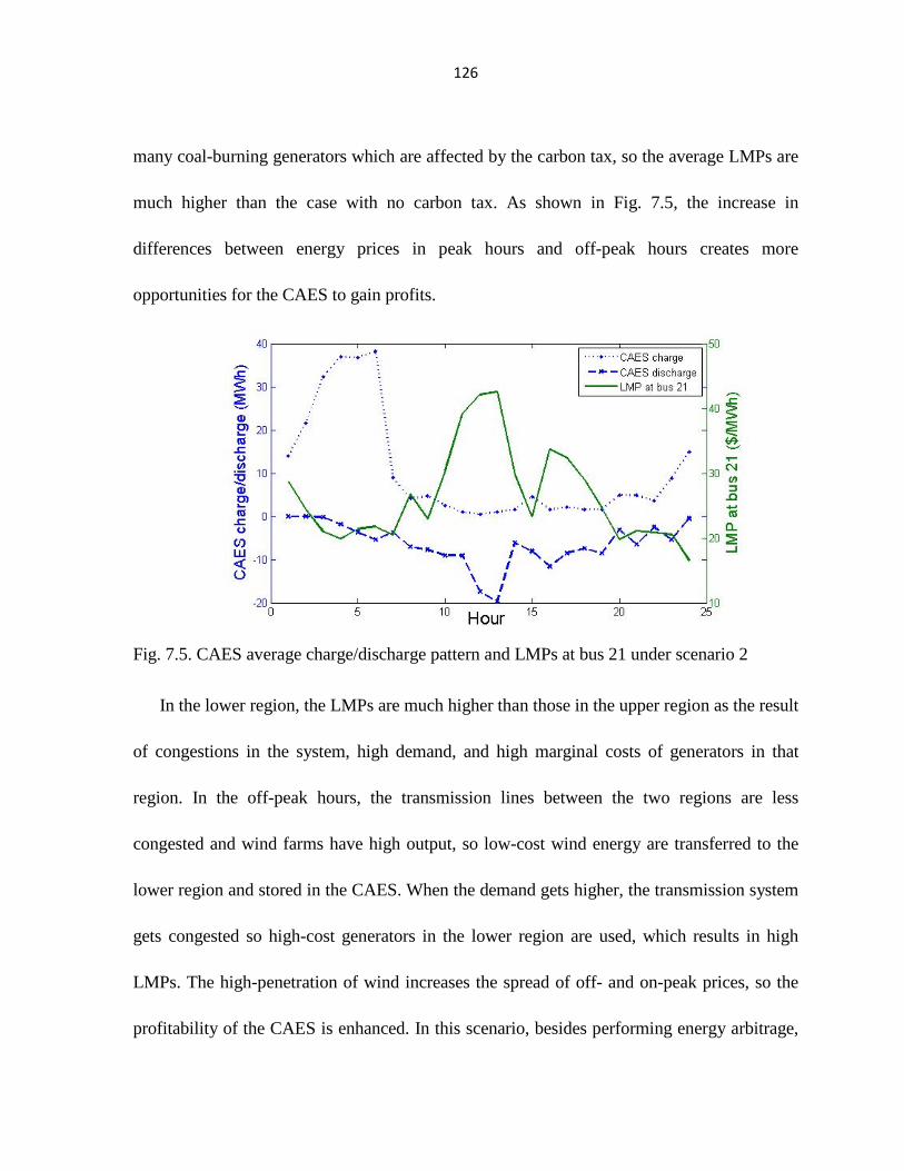
126
many coal-burning generators which are affected by the carbon tax, so the average LMPs are
much higher than the case with no carbon tax. As shown in Fig. 7.5, the increase in
differences between energy prices in peak hours and off-peak hours creates more
opportunities for the CAES to gain profits.
Fig. 7.5. CAES average charge/discharge pattern and LMPs at bus 21 under scenario 2
In the lower region, the LMPs are much higher than those in the upper region as the result
of congestions in the system, high demand, and high marginal costs of generators in that
region. In the off-peak hours, the transmission lines between the two regions are less
congested and wind farms have high output, so low-cost wind energy are transferred to the
lower region and stored in the CAES. When the demand gets higher, the transmission system
gets congested so high-cost generators in the lower region are used, which results in high
LMPs. The high-penetration of wind increases the spread of off- and on-peak prices, so the
profitability of the CAES is enhanced. In this scenario, besides performing energy arbitrage,
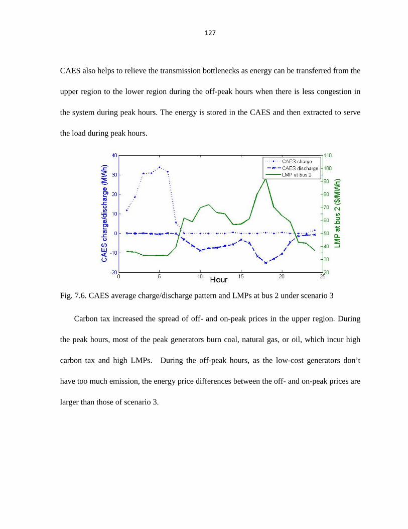
127
CAES also helps to relieve the transmission bottlenecks as energy can be transferred from the
upper region to the lower region during the off-peak hours when there is less congestion in
the system during peak hours. The energy is stored in the CAES and then extracted to serve
the load during peak hours.
Fig. 7.6. CAES average charge/discharge pattern and LMPs at bus 2 under scenario 3
Carbon tax increased the spread of off- and on-peak prices in the upper region. During
the peak hours, most of the peak generators burn coal, natural gas, or oil, which incur high
carbon tax and high LMPs. During the off-peak hours, as the low-cost generators don’t
have too much emission, the energy price differences between the off- and on-peak prices are
larger than those of scenario 3.

128
Fig. 7.7. CAES average charge/discharge pattern and LMPs at bus 2 under scenario 4
Besides providing electric energy, CAES can also provide high-value ancillary services
such as spinning and non-spinning reserves. Table 7.1 shows the CAES’s profits from the
energy and ancillary service markets. The CAES has the highest overall profit under
scenarios 4, possibly due to volatility in nodal prices and high gap between peak prices and
off-peak prices. As shown in the table, the CAES can gain a significant amount of profits
from the ancillary service market.
Table 7.1. Annual Profits of the CAES

129
A sensitivity analysis was conducted to evaluate the effects of CAES’s capacity on its
annual earning and total system production cost under scenario 3. In table 7.2, the CAES’s
profits first go up then go down as CAES’s capacity increases. When the CAES’s capacity is
twice as large as its original capacity, it can get more profits by providing energy and
spinning reserve. However, as CAES is bidding at its marginal cost, when CAES’s capacity
gets larger and larger, it can substitute the high cost units during the peak hours, resulting in
low peak hour prices. As the CAES is paid LMP for its energy, it will have less revenue.
When the CAES’s capacity is infinite, it will totally substitute the high-cost peak generators
and have fewer profits. As strategic bidding is not considered in this study, the actual profits
of the CAES should be higher.
The profitability of the CAES is affected by transmission congestions as if system is
congested all day long, the CAES cannot obtain enough low-cost energy from the upper

130
region, which interferes the energy arbitrage function of the CAES. In table 7.2, when there
is no transmission limits in the system, the total production costs reduced a lot.
Table 7.2. CAES’s Annual Profits and System Total Production Costs V.S. CAES Capacity
The results showed that CAES can provide both energy and reserves, reduce the carbon
dioxide emission and promote the efficient use of wind energy. For that particular system, the
case study showed that CAES could get the higher profits when it was located near the load
center. Carbon tax also had some effects on CAES’s profitability, but not too much.
As the regulating reserve is not considered in the study, this analysis only shows the
lower bound of CAES’s profits. As wind causes a lot of variation in the supply side, many
thermal units need to constantly vary their generation outputs to maintain the frequency
stability. The excessive cycling of these coal- and natural gas- fired units will cause aging
and extra maintenance costs. As wind penetration level gets higher and higher, these units

131
may bid higher regulating reserve prices in order to offset the extra cycling costs.
Fast-responding units such as CAES can benefit from this as they are designed to vary the
generation levels frequently at low costs.
The conclusion drawn from this case study about whether storage should be located near
the wind sites or load center is applicable to the test system only. The conclusion might be
different for another system with different load patterns, generation mix, fuel prices, or
transmission topology/constraints. However, the models proposed and analytical methods
employed in this study can be applied to various systems.
7.4 Comparing the Economic Performance of CAES and
Transmission Line Additions
As illustrated in previous chapters, both CAES and new transmission lines are bring
significant economic benefits if planned carefully, however, in order to evaluate the
possibility of building CAES to defer or even substitute transmission investments, a
systematic approach to compare the two investment plans needs to be designed. The
procedures to use the above proposed mid-term hourly production cost simulation model to
assess the two planning alternatives are shown below:
1) Evaluate system condition and propose candidate CAES investment projects.
2) Use the mid-term production cost simulation tool to simulate the operations of the
system and identify the best CAES candidate. Depending on the decision maker’s

132
preference, there can be multiple criteria for the candidate CAES projects such as
benefit/cost ratio, reduced load payments, reduced congestion costs, etc.
3) Evaluate system condition and propose candidate transmission investment projects.
4) Use the market-based transmission expansion planning tool to identify the best
transmission investment plan.
5) Use the mid-term production cost simulation tool to simulate the operations of the
system with the new transmission lines.
6) Assess the economic performance of the two set of plans by comparing their
benefit/cost ratios.

133
CHAPTER 8 THE MARKET-BASED TRANSMISSION
PLANNING TOOL
8.1 Introduction
The Market-based Transmission Expansion Planning (MBTEP) tool is written in
MATLAB/TOMLAB and uses CPLEX as the optimization engine. The system information
needs to be prepared using a .csv or .txt file following a specific format. After the input files
are ready, the preprocessor reads the input files and generates a MPS file for the master
problem and a MPS file for slave problem, random seed generators for the Monte Carlo
simulation, and the wind speed foresting model for wind. Then all the generated files are sent
to the model generator where the Benders decomposition and Monte Carlo simulation are
conducted. Once the final optimal solution is obtained, a solution report will be generated
containing information about the system information and investment plan. The MBTEP tool
can conduct long-term market-based transmission expansion planning and identify an
investment plan that can bring the maximum amount of net economic benefits to the system.
The general properties of the MBTEP tool include:
• Simulating the long-term operation of the electric system in flexible time steps
(5-minute, hourly, daily, monthly, annual)
• Simulating different parts of the electric system in different time steps, e.g. hourly
simulation time step for traditional generators, 5-min simulation time step for
wind and CAES.

134
• Simulating the operation of electric market with double-sided biddings
• Methodology to calculate the LMPs for all the buses, and MCP for spinning and
non-spinning reserves.
• Ability to simulate not only electric system but also related systems such as fuel
transportation system.
• Methodology to analyze the long-term economic performance of the system
• Methodology to analyze the long-term reliability performance of the system
• Ability to simulate the greenhouse gas emission, model emission constraints, and
include carbon tax in the model.
• Simulating the generation expansion planning problem from generation
companies’ perspective, i.e. maximize the expected value of (generation profits –
investment cost)
• Simulating the transmission expansion planning problem from ISO/RTO’s
perspective, i.e. maximize the expected value of (social surplus for the whole
market – investment cost)
• Methodologies that enable the users to identify/verify specific transmission
bottlenecks.
• Ability to easily calibrate the models and subsystems of the tools.
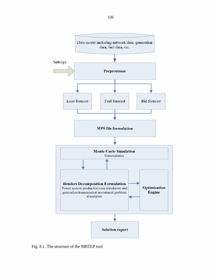
135
Fig. 8.1. The structure of the MBTEP tool

136
One concern with using this MBTEP tool on large system is the computation time.
Although this dissertation did not test the MBTEP tool on a big system, the structure of the
optimization problem makes it possible to solve the large planning problem in a reasonable
time. The total computation time is decided by three factors: the number of iterations,
computation time of the master problem in each iteration and computation time of the slave
problem in each iteration. Section 3.4.3 discussed this issue and analyzed the computation
time for the master and slave problems, respectively. One conclusion that can be drawn from
that section is that for a large system, the computation time is mainly decided by the number
of iterations and the slave problem. In order to reduce the iteration time, the hierarchical
decomposition method can be easily introduced in the MBTEP tool [86]. Hierarchical
decomposition method will first relieve some constraints from the slave problem (such as the
DC power flow constraints) and get the optimal solution set for the relaxed optimization
problem. Then this solution can be used as the starting point to get the final optimal solution
for the whole planning problem. With regard to the computation time of the slave problem,
the slave problem can be further decomposed and parallel computing technique can be
employed to make the computation time tractable. In summary, although the system capacity
expansion planning problem is very computation intensive, the formulation of the planning
model is very suitable to be combined with other techniques to make the computation time
on large systems reasonable.
8.2 Input Data

137
The MTEP tool uses the Generalized Network Flow method to model the whole system.
In the GNF formulation, the system is comprised of nodes and arcs. The detailed information
on the nodes and arcs of the system is included in the nodesinitial.csv and arcsinitial.csv.
In the nodesinitial.csv file, all of the nodes in the system and their properties are included.
The entries in the input file are: node name, the type of flow that go through the node (e.g.
coal, natural gas, electricity, oil, etc.), node type (e.g. a generation bus, a transmission bus,
etc.).
In the arcinitial.csv file, all of the arcs in the system and their properties are include.
Arcs are considered as the link between two nodes. Many processes such as generation, fuel
transportation, transmission can be treated as arcs with flows going through. There are 30
data entries in the arcsinitial.csv file. The data entries are: 1) Arc name (source node name +
sink node name), 2) Source node name, 3) Sink node name, 4) Type of flow, 5) Cost, 6)
Efficiency, 7) Minimum flow constraint, 8) Maximum flow constraints, 9) Number of arcs,
10) Investment cost (the expansion investment if applicable, otherwise it is 0), 11)
Susceptance (for transmission lines only, 0 for other kinds of arcs), 12) Whether it can
provide spinning) reserve or not (entries 12 to 28 are valid for arcs representing electric
generation processes only, 13) Whether it can provide non-spinning reserve or not, 14)
Ramp-up rate , 15) Ramp-down rate, 16) Start-up cost, 17) Shut-down cost, 18)/19)/20)
energy bidding segment 1 (minimum capacity, maximum capacity, cost), 21)/22)/23) energy
bidding segment 2, 24)/25)/26) energy bidding segment 3, 27) Spinning reserve bid, 28)

138
Non-spinning reserve bid, 29) Forced-outage rate, 30) Co2 emission coefficient, 32) whether
it can provide regulating reserve or not, 32) regulating reserve bid.
The employment of .csv files as input makes it possible to consider more properties of
nodes and arcs if needed. For example, if we need one more property for generator such as
regulating reserve bid, one more column can be added to the arcsinitial.csv file. The above
input files only consider the status of the system at the beginning of the planning horizon,
further information are required to capture the dynamic properties of the system such as load
level, fuel prices, generation capacities, etc.
8.3 Preprocessor
The preprocessing process read the input files about nodes and arcs and also the input
files about load data and wind data. Preprocessor also requires proper setting such as load
growth rate, fuel cost growth rate, generation maintenance schedule, planning horizon, time
step, etc. The outputs of the preprocessor are nodes.csv and arcs.csv, which contains the
system information over the whole planning horizon.
On interesting function of the preprocessor is that it can expand different subsystems of
the existing system using different time steps. Various energy subsystems have different
dynamics. For example, the wind speed is highly volatile, so in order the capture the impact
of wind output on the operation of the market, it makes sense to use a 5-min simulation time
step. The coal transportation subsystem, however, has a much lower dynamics as most of the
coal-burning power plants have long-term contracts with the fuel provider so a weekly or

139
monthly time step can be used for this subsystem. If a single simulation time step is used for
the whole system as many other system simulation tools do, that time step needs to be small
enough to capture the fastest dynamics in the system, which incurs huge computational
burden. Using various time steps to account for different dynamics helps to reduce the
computation time while capturing the unique operating characteristics of different
subsystems.
Fig. 8.2. The structure of the preprocessor
8.3 MPS file generation
Mathematical Programming System (MPS) is a file format to store optimization
problems. All major optimization engines accept this format, which make the MBTEP
flexible to the kind of optimization solver it uses. MPS file has a specific format to formulate
the optimization problem, as shown in Fig. 8.3. MPS is a column-oriented format and all of

140
the components of the optimization problem, such as variables, columns, rows, etc., have
unique names. Fig. 8.4 shows the equation-oriented format of the same optimization problem
as the one in Fig. 8.3. Most optimization engines have the ability to convert the MPS format
to the standard format. One advantage of the MPS format is that, compared to generating
huge matrices directly, it is easy to generate the MPS file based on the nodes.csv and arcs.csv.
For example, in order to generate the generation/load balance equations for all the buses, first,
the list of buses are read from the nodes.csv and n (n is the number of buses) rows are
defined; then for each buses, all of the connected arcs are identified in the arcs.csv and the
“COLUMNS” section can be created by assigning coefficients (1 for input arc and -1 for
output arc if loss is not considered) to the arcs; finally, the “RHS” section can be generated
by entering the load for each bus.

141
Fig. 8.3. The MPS file format
Fig. 8.4. The same optimization problem written in equation-oriented format
8.4 Optimization model
8.4.1 Benders Decomposition and Monte Carlo Simulation
One of the important features of the MBTEP is that Benders Decomposition is employed
to split the whole optimization problem into sub-problems and solve them iteratively. This
formulation of the planning problem can: 1) Enable the optimization server to solve what
previously are unsolvable problems. For instance, the CPLEX solver cannot solve
mixed-integer non-linear problem. By dividing the whole problem into a mixed-integer
problem and a non-linear problem, the optimal solution can be obtained. 2) Reduce the
computation time. 3) Obtain the dual solution of the slave problem and use it in the master.
For instance, in the overall planning problem, it is not possible to consider the LMPs of the
buses in the objective function because LMPs is a byproduct of the optimization problem.
Benders Decomposition enables the usage of LMPs to calculate the generators’ profit in the
objective function of the master problem. 4) Use several system performance evaluation

142
sub-systems to capture various aspects of the operation of the system. For example, there can
be two sub-problems in the MBTEP tool, the system production cost simulation sub-problem
and the system reliability evaluation sub-problem. It is also possible to include other
sub-problems to assess other aspects of the operation.
The operation of the electric market is strongly related to physical characteristics of the
power system such as loads, fuel prices, hydrological conditions, national energy policy,
wind energy output, transmission capability, emission allowances, and unit operating
characteristics. Another important feature of the MBTEP tool is the employment of Monte
Carlo method to account for the various uncertainties associated with parameters of the
planning model. By combining Benders Decomposition method and Monte Carlo simulation
technique, the MBTEP can analyze the long-term operations of the electric system and make
investment decisions based on numerous simulations of possible states of the system. The
flow chart of the Bender Decomposition and Monte Carlo simulation processes is shown in
Fig. 8.5.
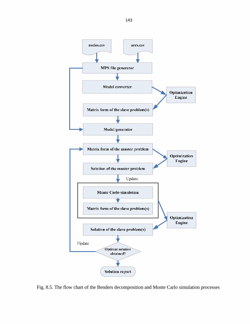
143
Fig. 8.5. The flow chart of the Benders decomposition and Monte Carlo simulation processes

144
8.4.2 System Long-term Performance Evaluation
Making the wise transmission and/or generation expansion investment plan involves
extensive evaluation of the performance of the electric power system over the whole
planning scope. The slave problems of the TEP and GEP models make the long-term system
performance evaluation. Currently, there are two kinds of the slave problems in the MBTEP,
as shown in Fig. 8.6. The first slave problem assesses the economic performance of the
electric market; the second slave problem assesses the reliability of the electric system. The
MBTEP can be configured to use either one, or both of the slave problems. The structure of
the MBTEP also makes it possible to include other user defined slave problems or
constraints.
The economic assessment slave problem simulates the operation of the electric/ancillary
market with double-sided biddings. The UC and ED problems are solved hourly in order to
simulate the day-ahead market. This slave problem has the capability of producing the
following results:
• Locational Marginal Prices for all of the electric buses.
• Nodal prices for all of the nodes in the fuel subsystem (if applicable).
• Market Clearing Prices for the spinning and non-spinning reserves.
• Detailed hourly generation, transmission, and storage information.
• Detailed commitment schedules of the generation fleet.
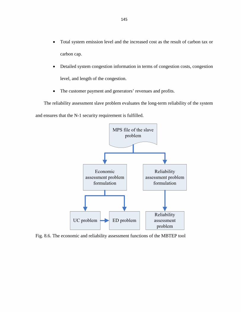
145
• Total system emission level and the increased cost as the result of carbon tax or
carbon cap.
• Detailed system congestion information in terms of congestion costs, congestion
level, and length of the congestion.
• The customer payment and generators’ revenues and profits.
The reliability assessment slave problem evaluates the long-term reliability of the system
and ensures that the N-1 security requirement is fulfilled.
MPS file of the slave
problem
Economic
assessment problem
formulation
Reliability
assessment problem
formulation
UC problem
Reliability
assessment
problem
ED problem
Fig. 8.6. The economic and reliability assessment functions of the MBTEP tool

146
CHAPTER 9 CONCLUSION
9.1 Contributions
• Proposed a new transmission planning methodology, compared it with the traditional
planning models, and validated it advantage over existing models by conducting the
case study.
• Implemented the market-based transmission planning method and built a planning
tool.
• Proposed a transmission planning methodology that took both the reliability and
economic criteria into consideration.
• Employed Benders decomposition method to reduce the computation time and
employed Monte Carlo simulation/robustness testing methods to incorporate various
uncertainties in the planning model.
• Used generalized network flow model to represent the energy flow in both the electric
system and the fuel network.
• Built models for wind farms and storage facilities and incorporated them into the
planning model.
• Implemented the co-optimization of both the energy market and ancillary service
market in the transmission planning model so that the impacts of increasing wind
penetration level on the operating reserve can be evaluated.
147
• Proposed a new transmission planning methodology that can simulate the interactions
between large scale wind integration and transmission expansion planning.
• Designed a systematical way to evaluate the possibility of building energy storage
system to defer or substitute the transmission expansion investments.
9.2 Further Research Directions
Further research might be done in a variety of directions based on the proposed research
work in the dissertation. Some of the interesting ideas for further research are shown below.
• Employing parallel computing algorithm in the MBTEP tool. One of the major
issues with the optimization model of transmission expansion planning is the
significant computation time. As the transmission expansion planning problem is a
mix-integer non-linear optimization problem, the computational complexity of the
model would be as bad as NP-hard (non-deterministic polynomial-time hard). In
order to reduce the computational time, computer technologies such as parallel
computing can be employed. Parallel computing is used in a wide range of fields,
from bioinformatics (protein folding and sequence analysis) to economics
(mathematical finance). Combining parallel computing algorithm and transmission
expansion planning model might significantly reduce the computation time and
enable the proposed model to be applied on larger systems.
• Using statistical model to forecast the long-term wind speed. Wind turbine
generator’s output is highly volatile as the result of constantly changing wind speed

148
and direction. In order to forecast the wind speed, many mathematical models were
formulated, such as ARMA model, multi-variable statistical model, neural network
model, etc. Wind speed model, combined with detailed wind turbine output model,
generate the wind power generation at each time step. While lots of efforts have been
made to simulate and forecast the wind output, there are still big errors in the forecast.
In order to capture the long term patterns as well as short-term variations of the wind
speed, multi-variable statistical model and ARMA model can be used together in the
production cost simulation problem. Multi-variable statistical model can be used to
forecast the wind output for the next twenty-four hours in the day-ahead market. In
the day-ahead market, the UC and ED models decide the commitment and dispatch
schedule for the next day based on the wind generation forecast from the
multi-variable statistical model. Then in the real-time market, the sequential Monte
Carlo simulation method can be employed to account for the uncertainties the wind
generation output. In order to capture the wind forecast errors, multiple wind
generation forecast can be generated by the ARMA model based on the forecasted
values used in the day-ahead market. Then the production cost model simulates the
operation of the real-time market for a large number of times. In each simulation, a
new wind generation forecast is generated by the ARMA model. The proposed model
can properly consider not only the annual, seasonal, weekly, or hourly patterns, but
also the sub-hourly fluctuations of the site-specific wind speed variations.

149
• Analyzing the interactions between the fuel transportation system and the
electric system. Fuel price is a major component of the generating units’ marginal
cost. The fluctuation of the fuel price will significantly impact the LMPs, unit
commitment schedule, dispatch schedule, and economic benefits. For example, in
many electric systems, sometimes the oil-burning units are the marginal units in the
peak hours, so the market clearing prices are mainly decided by the oil prices. The
fuel prices that generators see are mainly comprised of two components: the raw fuel
price and the transportation/storage cost. The fuel transportation will affect the fuel
prices that generators pay, and final the LMPs in the market. Investigating the
interactions between fuel transportation system and electric power can provide
valuable information about the long-term fuel price forecast and uncertainty with the
fuel price.
• Capturing the impacts of emerging technologies on the system expansion
planning model. With the advancement of technologies and applications such as
demand-side management, distributed generation, and plug-in hybrid vehicles, the
future demand level and shape will be changed. The system expansion planning tool
needs to consider the impacts of these new technologies on the economic
performance and reliability of the system.
• Evaluating the impacts of changes in national renewable energy policies on
system expansion planning problem. In the past decodes, wind has been the fastest

150
growing electric power source in U.S. The rising costs of fossil fuels, improvements
in renewable energy technologies, growing number of states enforcing renewable
portfolio standards (RPS), prospect of future carbon regulations and federal
production tax credit (PTC) have been the major driver of the growth of renewable
energy. Despite the significance of national/state renewable policies on wind energy,
little efforts have been made to analyze their impacts on the long-term electric system
expansion outcome. Energy policies such as PTC, carbon tax and/or carbon cap and
trade will change the GenCo and TransCo’s expectations on their future profits and
consequently their investment strategies. It is very important to assess the influence of
possible major national/state energy policies on the system capacity expansion
planning problem.
• Evaluate the impacts of large-scale wind power on the operations of the system
and the possible way to fix the issues. Wind energy will have substantial growth in
the decade ahead as the result of aggressive wind penetration level and on-shore and
off-shore wind potential. Although the variability of wind energy and the significant
wind forecast errors in the day-ahead and real-time markets can be partially
accommodated by existing operational procedures, the increasing wind penetration
level will challenge system operators regarding the procurement of enough ancillary
services. Studies need to be carried out to analyze the impact of high wind penetration
on the electric market. What is more, possible solutions to that issue such as CAES

151
should also be evaluated. To thoroughly analyze the operating characteristics of
CAES and wind power and how they perform in the energy and ancillary service
market, a simulation tool which co-optimize the two markets and simulate the system
at a 5-min time step is required.
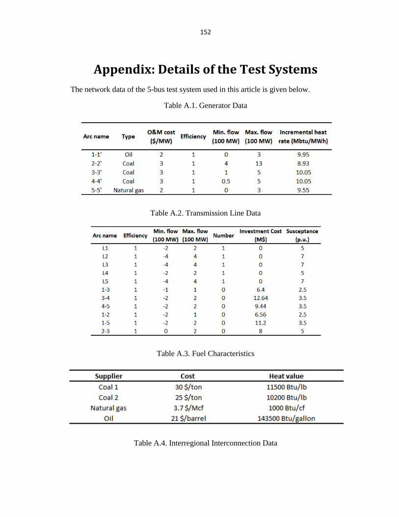
152
Appendix: Details of the Test Systems
The network data of the 5-bus test system used in this article is given below.
Table A.1. Generator Data
Table A.2. Transmission Line Data
Table A.3. Fuel Characteristics
Table A.4. Interregional Interconnection Data
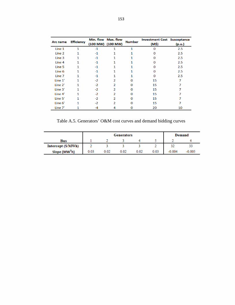
153
Table A.5. Generators’ O&M cost curves and demand bidding curves

154
BIBLIOGRAPHY
[1] M. Buygi, G. Balzer, H. Shanechi, and M. Shahidehpour, “Market-based transmission expansion
planning,” IEEE Trans. on Power Syst., vol. 19, no. 4, November 2004.
[2] Department of Energy, National Transmission Grid Study. May 2002.
[3] U.S. Department of Energy, Transmission Bottleneck Project Report. March 2003.
[4] G. B. Shrestha and P. A. J. Fonseka, “Congestion-driven transmission expansion in competitive
power market,” IEEE Trans. on Power Syst., vol. 19, no. 3, August 2004.
[5] Sevin Sozer, Chan S. Park, and Jorge Valenzuela, “Economic analysis of electric power
transmission expansion,” The Engineering Economist, 53:293--317, 2008.
[6] S. Wang, J. Zhu, L. Trinh, and J. Pan, “Economic assessment of HVDC project in deregulated
energy markets,” DRPT, April 2008.
[7] J. Roh, M. Shahidehpour, and L. Wu, “Market-based generation and transmission planning with
uncertainties,” IEEE Trans. on Power Syst., vol. 24, no. 3, August 2009.
[8] Consortium of Electric Reliability Technology Solutions, Economic evaluation of transmission
interconnection in a restructured market, California ISO, June 2004.
[9] J. F. Benders, “Partitioning procedures for solving mixed-variables programming problems,”
Journal Numerische Mathematik, vol. 4, no. 1, pp. 238–252, Dec. 1962.
[10] A. M. Geoffrion, “Generalized benders decomposition,” Journal of Optimization Theory and
Applications, vol. 10, no. 4, pp. 237–260, Oct. 1972.
[11] S. Binato, M. Pereira, S. Granville, “A new Benders Decomposition Approach to Slove Power
Transmission Network Design Problems,” IEEE Trans. on Power Syst., vol. 16, no. 2, May 2001.

155
[12] Y. Li and J. McCalley, “A General Benders Decomposition Structure for Power System Decision
Problems,” IEEE International Conference on Electro/Information Technology, EIT 2008.
[13] Douglas Hubbard, How to Measure Anything: Finding the Value of Intangibles in Business, John
Wiley & Sons, 2007
[14] Midewest ISO, Midwest ISO Transmission Expansion Plan 2009, December 2009
[15] H. Stoll, “Least-cost electric utility planning,” 1989, John Wiley.
[16] Hobbs BF. “Optimisation methods for electric utility resource planning,” Eur J Operational
Research, 1995
[17] C.K. Pang; G.B. Sheble, and F. Albuyeh, “ Evaluation of Dynamic Programming Based
Methods and Multiple area Representation for Thermal Unit Commitments,” IEEE Transactions on
Power Apparatus and Systems, March 1981.
[18] Y. Gu, J. McCalley, and M. Ni, “Coordinating Large-scale Wind Integration and Transmission
Planning,” submitted to IEEE Trans. On Renewable Energy, 2011
[19] N. Nabona, “Multicommodity Network Flow Model for Long-Term Hydro-Generation
Optimization”, IEEE Trans. on Power System. Vol. 8, No. 2, May 1993.
[20] N. J. Balu, R. Adapa, G. Cauley, M. Lauby, and D. J. Maratukulam, “Review of Expert Systems
in Bulk Power System Planning and Operation”, Proceedings of the IEEE, Vol. 80, No. 5, May 1992.
[21] K. P. Wong. “Artificial Intelligence and Neural Network Applications in Power Systems”, IEE
Second International Conference on advances in Power System Control, Operation and Management.
Hong Kong,December 1993.
[22] Y. Fukuyama, and H. Chiang, “A parallel genetic algorithm for generation expansion planning,”
IEEE Transactions on Power System, Vol. 11, May 1996.

156
[23] J. Barquín, E. Centeno and J. Reneses . “Stochastic market equilibrium model for generation
planning,” Probability in the Engineering and Informational Sciences, 19, pp 533-546, 2005
[24] F. F. Wu, F. L. Zheng, and F. S. Wen, “Transmission investment and expansion planning in a
restructured electric market,” J. Energy, 2006
[25] Y.P. Dusonchet, and A. El-Abiad, “Transmission Planning Under Discrete Dynamic
Optimizating,” IEEE Trans. On Power Apparatus and Systems, Vol. PAS-92, Jan. 2007.
[26] J. Contreras and F. F.Wu, “A kernel-oriented algorithm for transmission expansion planning,”
IEEE Trans. Power Syst., vol. 15, pp. 1434–1440, Nov. 2000.
[27] H. Sun and D. C. Yu, “A multiple-objective optimization model of transmission enhancement
planning for independent transmission company (ITC),” Proc. IEEE Power Eng. Soc. Summer
Meeting 2000, vol. 4, pp. 2033–2038.
[28] E. Handschin, M. Heine, D. König, T. Nikodem, T. Seibt, and R. Palma, “Object-oriented
software engineering for transmission planning in open access schemes,” IEEE Trans. Power Syst.,
vol. 13, pp. 94–100, Feb. 1998.
[29] F. E. N. Nasser, A. P. A. Silva, and L. A. P. Araujo, “Development of an expert system for
long-term planning of power transmission networks,” in Proc. 2nd Symp. Experts Syst. Applicat.
Power Syst., Jul. 1989, pp. 237–242.
[30] Y. Gu and J. McCalley, “Market-based Transmission Planning Considering Large-scale Wind
Power,” in Proc. The International Workshop on Large-Scale Integration of Wind Power into Power
Systems as well as on Transmission Networks for Offshore Wind Power Plants, Québec, Canada,
October 2010.
157
[31] Y. Gu and J. McCalley, “Market-based Transmission Expansion Planning,” in Proc. IEEE PES
Power Systems Conference & Exhibition (PSCE), Phoenix, Arizona, March 2011.
[32] Y. Gu and J. McCalley, “Market-based Transmission Expansion Planning With Uncertainty,” in
Proc. North American Power Symposium, Arlington, Texas, September 2010.
[33] G. Latorre-Bayona and I. J. Pérez-Arriaga, “Chopin, a heuristic model for long term transmission
expansion planning,” IEEE Trans. Power Syst., vol. 9, pp. 1886–1894, Nov. 1994.
[34] H. K. Youssef and R. Hackam, “New transmission planning model,” IEEE Trans. Power Syst.,
vol. 4, pp. 9–18, Feb. 1989.
[35] L. Bahiense, G. C. Oliveira, M. Pereira, and S. Granville, “A mixed integer disjunctive model for
transmission network expansion,” IEEE Trans. Power Syst., vol. 16, pp. 560–565, Aug. 2001.
[36] International Atomic energy agency, ‘’Enhanced electricity system analysis for decision
making‘’, 2000
[37] GenTrader website: http://www.powercosts.com/products/gentrader.asp
[38] J. Bastian, J. Zhu, V. Banunarayanan, and R. Mukerji, “Forecasting
Energy Prices in a Competitive Market,” IEEE Computer Applications in Power Magazine, vol. 12,
no. 3, pp. 40-45, July 1999.
[39] V. Koritanov, T. Veselka, “Modeling the regional electricity network in Southeast Europe,” Pwr
Engr Society General Meeting, Volume 1, July 2003 .
[40] Promod Website: http://www1.ventyx.com/analytics/promod.asp
[41] ProSym website: http://www.ventyx.com/analytics/market-analytics.asp

158
[42] W. Head, H. Nguyen, et al “The procedure used to assess the long range generation and
transmission resources in the Mid-Continent Area Power Pool,” IEEE Transactions on Power
Systems, Volume 5, Nov. 1990
[43] PLEXOS website: http://www.energyexemplar.com
[44] H. Yamin, J. Finney, W. Rutz and H. Holly, “GENCOs portfolio management using
“STRATEGIST” in deregulated power markets,” Large Engineering Systems Conference on Power
Engineering, July 2001.
[45] WASP-IV model documentation: http://www.adica.com/wasp_iv.html
[46] M. Lu, Z. Dong,T. Saha, “A Framework for Transmission Planning in a Competitive Electricity
Market,” Proc. of the Transmission and Distribution Conference and Exhibition: Asia and Pacific,
2005 IEEE/PES 2005, pp 1-6.
[47] MARS website:
www.gepower.com/prod_serv/products/utility_software/software/en/ge_mars.htm.
[48] TPLAN website: http://www.pti-us.com/pti/software/tplan/index.cfm
[49] T. Tran, J. Kwon, J. Choi, D. Jeon and K. Han, “Sensitivity Analysis of Probabilistic Reliability
Evaluation of KEPCO System Using TRELSS, ” International Conf on Probabilistic Methods
Applied to Power Systems, 2006.
[50] Eduardo Ibanez, “A multiobjective optimization approach to the operation and investment of the
national energy and transportation systems,” Ph. D dissertation, Iowa State University, 2011.
[51] A. Quelhas, E. Gil, J. D. McCalley, and S. Ryan, “A multiperiod generalized network flow
model of the U.S. integrated energy system part I- model description,” IEEE Trans. on Power Syst.,
vol. 22, no. 2, 2007.

159
[52] H. He, Z. Xu, “Transmission Congestion and its Social Effects,” IEEE PES., vol. 1, pp. 350- 354,
June 2005.
[53] R. Romero, A. Monticelli, “A hierarchical decomposition approach for transmission network
expansion planning,” IEEE Trans. on Power Syst., vol. 9, no. 1, Feburary 1994.
[54] J. Nicolaisen, V. Petrov, and L. Tesfatsion, “Market Power and Efficiency in a Computational
Electricity Market With Discriminatory Double-Auction Pricing,” IEEE Transactions on Evolutional
Computation, vol. 5, no. 5, October 2001.
[55] S. Ryan, A. Downward, A. Philpott, and G. Zakeri, “Welfare Effects of Expansions in
Equilibrium Models of an Electricity Market With Fuel Network.” IEEE Trans Pwr Sys., August
2010.
[56] C. H. Papadimitriou, “On the complexity of integer programming,” Journal of the ACM (JACM),
1981
[57] Cobham, Alan, "The intrinsic computational difficulty of functions," Proc. Logic, Methodology,
and Philosophy of Science II. North Holland, 1965
[58] Joint Coordinated System Plan ( JCSP). Available online: http://www.jcspstudy.org/.
[59] M. K. Kozlov, S. P. Tarasov and L. G. Khachiyan,. "Polynomial solvability of convex quadratic
programming," Doklady Akademii Nauk SSSR, vol. 248, 1049-1051. Translated in: Soviet
Mathematics - Doklady 20: 1108-1111, 1979
[60] Midwest ISO, Midwest ISO Transmission expansion plan 2010, Jan. 2011
[61] B.G. Gorenstin, N.M. Campodonico, J.P. Costa, and M.V.F. Pereira, “Power system expansion
planning under uncertainty,” IEEE Trans. Pwr. Sys., Volume 8, Issue 1, Feb. 1991.
[62] H. M. Merrill and A. J. Wood, “Risk and uncertainty in power system planning,” International
Journal of Electrical Power & Energy Systems, Volume 13, Issue 2, April 1991.

160
[63] A.P. Douglas, A.M. Breipohl, F.N. Lee, and R. Adapa, “Risk due to load forecast uncertainty in
short term power system planning,” IEEE Trans, Pwr. Sys., Volume 12, Issue 4, Nov. 1998.
[64] I.J. Silva, M.J. Rider, R. Romero, and C.A.F. Murari, “Transmission Network Expansion
Planning Considering Uncertainty in Demand,” IEEE Trans, Pwr. Sys., Volume 21, Issue 4, Nov.
2006.
[65] C. P. Robert, G. Casella, Monte Carlo Statistical Methods (2nd ed.). New York: Springer, 2004.
[66] G. Infanger, “Monte Carlo (Importance) Sampling within a Benders Decomposition Algorithm
for Stochastic Linear Programs,” TECHNICAL REPORT SOL 91-6, Annals of Operations Research,
1992
[67] George Casella and Roger L. Berger. Statistical Inference. Duxbury Press, 1990.
[68] E.O. Crousillat, P. Dorfner, P. Alvarado, H.M. Merrill, “Conflicting objectives and risk in power
system planning,” IEEE Trans. Pwr. Sys., Volume 8, Issue 3, Aug. 1993.
[69] H. M. Merrill, “Regional transmission organizations: FERC Order 2000,” IEEE Power
Engineering reviews, vol. 20, July 2000.
[70] H. Bludszuweit, J. A. Dominguez-Navarro, and A. Llombart, “Statical Analysis of Wind Power
Forecasr Error,” IEEE Trans. Power Syst. Vol. 23, No. 3, August 2008.
[71] A. Boone, “Simulation of short-term wind speed forecast errors using a multi-variate ARMA(1,1)
time-series model,” M.Sc. thesis, Royal Inst.Technol., Stockholm, Sweden, 2005.
[72] P. Pinson, H. Madsen, H. Nielsen, G. Papaefthymiou, and B. Klock, “From probabilistic
forecasts to statistical scenarios of short-term wind power production,” Wind Energy, Vol. 12, Issue 1,
pp 51–62, January 2009.
[73] D. J. Burke and M. J. O’Malley, “Maximizing Firm Wind Connection to Security Constrained
Transmission Networks,” IEEE Trans. Power Syst. Vol. 25, No. 2, May 2010

161
[74] K. W. Cheung, P. Shamsollahi, D. Sun, J. Milligan, and M. Potishnak, “Energy and Ancillary
Service Dispatch for the Interim ISO New England Electricity Market,” IEEE Trans. Power Syst. Vol.
15, No. 3, Aug. 2000.
[75] California ISO, “Spinning Reserve and Non-Spinning Reserve.” available online
http://www.caiso.com/docs/2003/09/08/2003090815135425649.pdf
[76] Reliability Test System Task Force of Probability Methods Subcommittee, “IEEE reliability test
system,” IEEE Trans. PAS-98, pp. 2047-2054, 1979.
[77] L. E. Benitez, P. C. Benitez, and G. Cornelis van Kooten, “The economics of Wind Power with
Energy Storage,” Energy Economics, No. 30, pp 1973-1989, 2008.
[78] P. Denholm, R. Sioshansi, “The Value of Compressed Air Energy Storage with Wind in
Transmission-constrained Electric Power Sytems,” Energy Policy, No. 37, pp. 3149-3158, 2009.
[79] P. Denholm, E. Ela, B. Kirby, and M. Milligan, “The Role of Energy Storage with Renewable
Electricity Generation,” Technical Report, NREL/TP-6A2-47187, Jan. 2010.
[80] H. Lund, G. Salgi, “The Role of Compressed Air Energy Storage in Future Sustainable Energy
Systems,” Energy Conversion and Management, No. 50, pp 1172-1179, 2009.
[81] Emerging Energy Storage Technologies in Europe. Rapport Frost and Sullivan, 2003.
[82] H. Ibrahim, A. Ilinca, and J. Perron, “Energy Storage Systems-Characteristics and Comparisons,”
Renewable and Sustainable Energy Reviews, No. 12, pp. 1221-1250, 2008
[83] Y.V. Makarov, et.al. “Wide-Area Energy Storage and Management System to Balance
Intermittent Resources in the Booneville Power Administration and California ISO Control Areas,”
PNNL Report, June 2008. Available Online:
http://www.electricitystorage.org/images/uploads/docs/Wide_Area_EMS_Report_V7.pdf

162
[84] Succar, S. and R. Williams. “Compressed Air Energy Storage: Theory, Operation, and
Applications.” March 2008.
[85] All Island Grid Study, Workstream 4—Analysis of Impacts and Benefits, Irish Government
Department of Communications, Energy and Natural Resources/United Kingdom Department of
Enterprise, Trade and Investment, Jan. 2008. Available online:
http://www.dcenr.gov.ie/Energy/North-South+Co-operation+in+the+Energy+Sector/All+Island+Grid
+Study.htm.
[86] R. Romero, A. Monticelli, “A hierarchical decomposition approach for transmission network
expansion planning,” IEEE Trans. Pwr. Syst. Vol. 9, issue 1, Feb 1994.