long-term vegetation dynamics of african savannas at a
TRANSCRIPT

Aristides Moustakas: Long-term vegetation dynamics of African savannas at a landscape level.
Long-term vegetation dynamics of African savannas at a
landscape level
Dissertation
Zur Erlangung des akademischen Grades
doctor rerum naturalium (Dr.rer.nat.)
Vorgelegt dem Rat der Biologisch-Pharmazeutischen Fakultät
der Friedrich – Schiller - Universität Jena
von Aristides Moustakas
Geboren am 20. April 1976 in Athen, Griechenland
Jena, 2006
1

Aristides Moustakas: Long-term vegetation dynamics of African savannas at a landscape level.
2

Aristides Moustakas: Long-term vegetation dynamics of African savannas at a landscape level.
Gutachter: 1.:……………………………………………………………….. 2.:……………………………………………………………….. 3.:……………………………………………………………….. Tag der Doktorprüfung:………………………………………. Tag der öffentlichen Verteidigung:……………………………
3

Aristides Moustakas: Long-term vegetation dynamics of African savannas at a landscape level.
“… supposedly they were searching for lignite. Actually they were searching for freedom...” The song of Nikos Kazantzakis & Alexis Zorbas Traditional Cretan song.
…as for the dilatoriness that we are accused, you shouldn’t feel shame, because if now you hurry to start the war, it will take you very long to finish it as you will be unprepared. And at last hasn’t our city always been free and famous? This is a proof of a sedate wisdom, since we are the only ones that don’t become arrogant when we are successful neither despondent when we fail. If some others try to drive us, against our intention, to dangerous adventures by praising us we are not flattered, and if they want to upset us by using insincere accusations we are not irritated and we don’t change our mind. Our political wisdom as well as our war virtue is based at the rule of law. This is due to the fact that honour is connected with wisdom and bravery with the feeling of shame. Our city is ruled by the law because the way we are raised is not as refined as to make us condemn the law. On the contrary, it is as hard as it is necessary to make us respect the law. We are not amongst those people that do unnecessary things and pass easy judgements on the preparation of the enemy during peace time but they fall short during action time. We believe that our opponents are at least as well prepared as we are and that the turns of luck cannot be predicted with logic. We are always prepared to face our opponents assuming that they are always acting with a well prepared plan. Thus, we should not be based on the mistakes of our enemies but on the measures that we will take, and we shouldn’t believe that humans differ from each other so much. Excellent though, is only the one who is sensitive but also raised hard and with self-discipline… Speech of Arhidamos, King of the Spartans to the Spartan assembly in preparation to the war with Athens. Thoukydides History, Book A, 84-86.
4

Aristides Moustakas: Long-term vegetation dynamics of African savannas at a landscape level.
TABLE OF CONTENTS CHAPTER ONE: General Introduction 7 CHAPTER TWO: Long-term mortality patterns of a deep-rooted Acacia tree:
the middle class shall die! 14 CHAPTER THREE: The paradox of climate-dependent growth in one of the
world’s deepest-rooted trees, Acacia erioloba 29 CHAPTER FOUR: Tree spacing patterns of an Acacia tree in the Kalahari over
61-year time replicate: how clumped becomes regular and vice versa! 47
CHAPTER FIVE: A spatially explicit savanna model along a soil and
precipitation gradient. Are savannas cyclothymiacs? 62 CHAPTER SIX: General Discussion 89 Summary: 94 Deutsche Zusammenfassung: 95 Acknowledgements: 97 Statement (Erklärung): 98 Curriculum Vitae (Lebenslauf): 99
5

Aristides Moustakas: Long-term vegetation dynamics of African savannas at a landscape level.
CHAPTER 1: General Introduction.
Overview
Savannas are ecosystems comprised of a mixture of two life forms, woody species
(trees and bushes) and grasses. Savannas cover about 13% of the global land surface and about half of the area of Africa, Australia, and South America (Scholes & Archer 1997). Till early 1990’s it was generally believed that trees and grasses coexist due to a separation of rooting niches (Sankaran et al. 2004). This idea was based on Walter’s two-layer hypothesis (Walker et al. 1981). According to this hypothesis, water is the limiting factor for woody species as well as grasses. Due to the fact that woody species can develop deep roots, it was assumed that grasses use only topsoil moisture, while woody species use subsoil resources. While there have been several studies concluding that savanna stability is based on the two-layer hypothesis (e.g. Weltzin & McPherson 1997), several findings that disputed that theory were also reported (e.g. Jeltsch et al. 1996). Among others, recently, Ludwig et al. (2004) reported a field experiment where the two-layer hypothesis is not valid. This means that rooting niche separation fails to generally explain savanna tree-grass coexistence.
As the niche separation hypothesis was invalid in several cases, new hypotheses were proposed in order to explain savanna stability and woody-grass coexistence. One hypothesis is that disturbances are key determinants of savannas. According to this hypothesis, savannas are lastingly unstable ecosystems due to the fact that they are under frequent or constant disturbances and perturbations. Ideally, in the absent of such disturbances, a savanna would turn into a woodland (forest) or into a grassland (Scholes & Archer 1997). A significant factor of disturbance is claimed to be fire (Higgins et al. 2000). According to this claim, fire intensity and frequency in combination with climatic factors determine the savanna physiognomy.
A common phenomenon in savannas is the increase of woody species often referred as “bush encroachment”. Bush encroachment is the increased dominance of woody species, mainly thorny bushes, which suppress grasses. Bush encroachment is usually characterised by the dramatic increase of species of thorny bushes. Bush encroachment is a serious problem reported in many geographically different savanna ecosystems. Drastic increase of woody species is a phenomenon observed in African (O’Connor & Crow 2000) as well as in American (Archer 1989) and Australian (Burrows et al. 1990) savannas. This increase of woody species is a serious problem in savannas because many herbaceous plants are suppressed or lost, and as a result, biodiversity is decreased. Furthermore, the density of woody species is often very high and reduces savanna carrying capacity, which has a direct effect on local mammalian herbivores as well as on domestic livestock which are unable to pass through or survive in such places (Scholes & Archer 1997).
There have been attempts to explain the causes of bush encroachment. One of them is based on the evidence that increasing levels of global CO2 favor the growth of trees and bushes which are C3 species rather than grasses which are mainly C4 species (Knapp 1993). However the validity of this theory was significantly reduced by the findings of
6
Aristides Moustakas: Long-term vegetation dynamics of African savannas at a landscape level.
Archer et al. (1995). Other theories combining fire with low atmospheric CO2 have been proposed (Bond et al. 2003) however they have not been verified with field studies.
A second alternative theory attempting to explain the increase of woody thorny species was based on Walter’s two-layer hypothesis. According to this theory, grass removal by heavy grazing allows more water to penetrate in the deep soil and thus more available water for woody plant growth. Despite the fact that the validity of Walter’s two-layer hypothesis is diminished, several studies explained the increase of woody species based on heavy grazing (e.g. Skarpe 1990). However, bush encroachment in areas where soil depth is too low to allow niche differentiation between woody and grassy species has been reported (Wiegand et al. 2005). As a result, apart from the fact that this theory is built on a problematic presupposition (two-layer hypothesis), the validity of this explanation is very limited.
According to disturbance theory of savanna stability, fire plays a key role for tree-grass coexistence (Higgins et al. 2000). However this theory is based on the presupposition that there is sufficient fuel load to support frequent and extensive fires (Belsky 1990; Ward 2005). While there is sufficient evidence that humid savannas could be fire-dominated, there is no such evidence in semi-arid or arid savannas where fires are not frequent and do not cover large spatial scales (Belsky 1990; Ward 2005). Thus, fire is not the driving factor in mesic and arid savannas and its general applicability to explaining bush encroachment fails to live up to the reality. The fact that disturbance theory fails to explain generation and persistence of bush encroached sites, questions also the general applicability of this theory on tree-grass coexistence and savanna stability.
Summing up, despite the fact that savannas cover 13% of land surface, the driving forces of savanna ecology remain mainly unknown. Furthermore the globally reported increase of woody species in savannas, is not well understood (Ward 2005). As a result there is a need for a new theory explaining savanna dynamics. Recently, Gillson (2004a; 2004b) and Wiegand et al. (2005; 2006) developed the idea that savannas are patch dynamic systems. According to the patch dynamics hypothesis, savannas are patch-dynamic systems composed of many patches in different states of transition between grassy and woody dominance. In arid savannas, key factors for patches are rainfall, which is highly variable in space and time, and intra-specific tree competition. According to the savanna patch dynamics theory, bush encroachment is part of a cyclical succession between open savanna and woody dominance. The conversion from a patch of open savanna to a bush-encroached area is initiated by the spatial and temporal overlap of several (localized) rainfall events sufficient for germination and establishment of woody species (trees & bushes). With time, growth and self-thinning will transform the bush-encroached area into a mature woody species stand and eventually into open savanna again. Patchiness is sustained due to the local rarity (and patchiness) of rainfall sufficient for germination of woody plants as well as by plant-soil interactions. According to this hypothesis, there is a spatial and temporal variation of the savanna facies. Temporally, a specific patch will pass through an encroached phase and sequentially to a more open savanna one, till it is encroached again. Spatially, when a savanna is viewed at a specific time step, there are some encroached patches, while some other patches are comprised of an open savanna (Wiegand et al. 2006). However, in order to validate or reject such a theory and possibly counter propose an alternative one, there is a need for long-term data on savanna plant demography.
7

Aristides Moustakas: Long-term vegetation dynamics of African savannas at a landscape level.
Demography of savanna plants Overview
The most common assumption in estimating tree age is that the largest trees are likely to be old (Harper 1977). Savanna tree life cycles are known to be long but are unquantified (Midgley & Bond 2001). Savannas in general and in particular African savannas are mainly dominated by Acacia species. Trees in non-temperate regions and particularly Acacia sp. in savannas may produce several growth rings in wet years and none in dry years (Gourlay & Kanowski 1991). Thus, plant age-size-growth-mortality relationships in savanna plants remain unclear. Due to the longevity of Acacia species and the absence of data, simulations have been used to estimate relationships between mortality and age or size in Acacia species but no such relationship was found (Wiegand et al. 2000).
Given that savannas cover a significant part of the global land surface, they play a significant role in climate change models (Privette et al. 2004). Due to the absence of data for savanna tree growth and mortality, models commonly either use a linearly-increasing relationship between tree size and mortality once a certain size threshold has been reached (e.g., Jeltsch et al. 1996), or consider mortality to be size-independent (e.g., Wiegand et al. 1999). Even though this seems to be a common assumption, it is not based on real field data.
Tree mortality
Mortality is an extremely important factor for understanding population dynamics and for management and yet, it is one of the most poorly-known processes in ecology (Zens & Peart 2003). Trees are usually long-lived organisms outliving researchers (Menges 2000). Causes of tree mortality apart from fire, wind, and diseases have seldom been quantified (Franklin et al. 1987). Specifically, slow-acting and cumulative natural causes of mortality are not well understood due to the difficulties involved in collecting long-term data (Menges 2000). Consequently, development of a theoretical approach to the relationship between tree size and mortality is slow (Hawkes 2000). There are no long-term studies on savanna tree mortality to our knowledge.
Tree growth
Unlike forests where light is a primary limiting resource, savanna tree growth is mainly limited by nutrients and water (Frost et al. 1986; Coomes and Grubb 2000). Thus, we expect forest species to allocate more resources aboveground to light capture and savanna species to capture mainly below-ground resources (Coomes and Grubb 2000, Hoffmann and Franco 2003). Savannas are more stressful and unproductive environments than forests and thus savanna trees grow slower (Chapin et al. 1993). Good studies on savanna tree growth have been conducted (e.g. Miller et al. 2001; Shackleton 2002; Hoffmann and Franco 2003). However, most of them are relative short-term studies
8

Aristides Moustakas: Long-term vegetation dynamics of African savannas at a landscape level.
covering up to 10 y time. There are no studies on long-term savanna tree growth to our knowledge. Spatial pattern analysis
A major problem in the study of vegetation dynamics in arid systems are the long time scales involved. Furthermore, these systems are typically event-driven (extreme droughts, rare germination) meaning that a study over 10 years may still miss important recruitment or dieback events and thus monitor practically unchanged vegetation. Patterns such as the spatial distribution of long-lived plants are archives of the history of the system. Thus, methods inferring information on long-term dynamics from snapshot patterns are extremely valuable. Understanding and explaining the underlying processes of the observed spatial patterns of plant individuals have long been an interesting question in plant ecology (Sterner et al. 1986). Spatial heterogeneity and interactions are important to the population dynamics of plants. Spatial influences such as plant competition or the distribution of safe sites for germination result in temporally variable spatial patterns of plant distribution (Kenkel 1988). If spatial processes of plant population dynamics have a strong influence on spatial patterns of plant distribution, then these spatial patterns necessarily contain information on population dynamics. Therefore, it should be possible to learn about population processes by investigating spatial patterns of plant distribution (Wiegand T. & Moloney 2004). Ecological Modelling
The use of modelling in ecology and other disciplines is a common tool to investigate questions that are difficult to investigate by field studies exclusively due to the absence of long or even medium-term data, time limitations and workforce. Much of the difficulty in savanna modelling and management arises from dealing with very different scales in time, space, and species interactions. Uneven spatial scales are particularly difficult to address using differential equations, because these models focus mainly on population dynamics but not on spatial distribution. Instead of than trying to add interaction mechanisms to models based on more uniform population dynamics, an alternate approach is to focus on the spatial distribution of trees, grass, and bushes, and to develop models which focus on the factors affecting plant growth based on their neighbouring situation. Good reviews of existing savanna models are given by Belsky (1990) and Sankaran et al. (2004). Aims and objectives
The main objective of this thesis was to study long-term, large-scale savanna vegetation dynamics. Specifically our main aims were:
• On a species level to study the demography (growth and mortality patterns) of Acacia erioloba, a key species in the Kalahari and in African savannas. A. erioloba is a deep-rooted, long-lived tree and thus appropriate for studying long-
9

Aristides Moustakas: Long-term vegetation dynamics of African savannas at a landscape level.
term tree mortality and growth. Our main field study area was located in the southern Kalahari, South Africa.
• To characterize spatial savanna dynamics. Specifically we aimed to examine scale-dependent tree spacing over time and space replicate.
• To build a computer model to simulate long-term savanna dynamics, using mainly published data. In contrast to most savanna simulation models, we wanted to study general savanna properties and we did not focus on a single place. As precipitation and soil properties are usually the limiting factors of savanna vegetation dynamics, we examined savanna vegetation dynamics on a precipitation and soil gradient.
Overall, we aimed to improve our understanding of savanna dynamics across scales.
We started at a species level (patch level), determined differences within patches, and finally simulated dynamics of different savannas at a landscape level consisting of many patches. References Archer S., Schimel D.S. & Holland E.A. (1995) Mechanisms of shrubland expansion:
land-use, climate or CO2? Climatic Change, 29, 91-99 Belsky A.J. (1990) Tree/grass ratios in East African savannas: a comparison of existing
models. Journal of Biogeography, 17, 483-489 Brown J.R. & Archer S. (1989) Woody plant invasion of grasslands: establishment of
honey mesquite (Prosopis glandulosa var. glandulosa) on sites differing in herbaceous biomass and grazing history. Oecologia, 80, 19-26
Brown J.R. & Archer S. (1999) Shrub invasion of grassland: recruitment is continuous and not regulated by herbaceous biomass or density. Ecology, 80, 2385-2396
Chapin, F.S., Autumn, K., Pugnaire, F. (1993). Evolution of suites of traits in response to environmental stress. American Naturalist (Suppl.), 142: S78–S92.
Coomes D.A. & Grubb P.J. (2000) Impacts of root competition in forests and woodlands: A theoretical framework and review of experiments. Ecological Monographs, 70, 171-207
Franklin J.F., Shugart H.H. & Harmon M.E. (1987) Tree death as an ecological process. BioScience, 37, 550-556
Frost, P., Medina, E., Menaut, J.-C., Solbrig, O., Swift, M., Walker, B. (1986). Responses of savannas to stress and disturbance. Biology International, Special Issue, 10: 1–82.
Gillson L. (2004a) Testing non-equilibrium theories in savannas: 1400 years of vegetation change in Tsavo National Park, Kenya. Ecological Complexity, 1, 281-298
Gillson L. (2004b) Evidence of hierarchical patch dynamics in an East African savanna? Landscape Ecology, 19, 883-894
Gourlay L.D. & Kanowski P.J. (1991) Marginal parenchyma bands and crystalliferous chains as indicators of age in African Acacia species. IAWA Bull., 12, 187-194
Harper J.L. (1977) Population biology of plants. Academic Press, New York, USA.
10

Aristides Moustakas: Long-term vegetation dynamics of African savannas at a landscape level.
Hawkes C. (2000) Woody plant mortality algorithms: description, problems and progress. Ecological Modelling, 126, 225-248
Higgins S.I., Bond W.J. & Trollope S.W. (2000) Fire, resprouting and variability: A recipe for grass-tree coexistence in savanna. Journal of Ecology, 88, 213-229
Hoffmann W.A. & Franco A.C. (2003) Comparative growth analysis of tropical forest and savanna woody plants using phylogenetically independent contrasts. Journal of Ecology, 91, 475-484
Jeltsch F., Milton S.J., Dean W.R.J. & Van Rooyen N. (1996) Tree spacing and coexistence in semiarid savannas. Journal of Ecology, 84, 583-595
Kenkel N.C. (1988) Pattern of self-thinning in jack pine: testing the random mortality hypothesis. Ecology, 69, 1017-1024
Ludwig F., Dawson T.E., Prins H.H.T., Berendse F. & Kroon H. (2004) Below-ground competition between trees and grasses may overwhelm the facilitative effects of hydraulic lift. Ecology Letters, 7, 623
Menges E.S. (2000) Population viability analyses in plants: challenges and opportunities. Trends in Ecology & Evolution, 15, 51-56
Midgley J.J. & Bond W.J. (2001) A synthesis of the demography of African acacias. Journal of Tropical Ecology, 17, 871-886
Miller D., Archer S.R., Zitzer S.F. & Longnecker M.T. (2001) Annual rainfall, topoedaphic heterogeneity and growth of an arid land tree (Prosopis glandulosa). Journal of Arid Environments, 48, 23-33
Noy-Meir I. (1982) Stability of plant-herbivore models and possible applications to savanna. In: Ecology of tropical Savannas (eds. Huntley BJ & Walker BH), pp. 591-609. Springer Verlag, Berlin and Heidelberg
Privette J.L., Tian Y., Roberts G., Scholes R.J., Wang Y., Caylor K.K., Frost P. & Mukelabai M. (2004) Vegetation structure characteristics and relationships of Kalahari woodlands and savannas. Global Change Biology, 10, 281-291
Sankaran M., Ratnam J. & Hanan N.P. (2004) Tree-grass coexistence in savannas revisited - insights from an examination of assumptions and mechanisms invoked in existing models. Ecology Letters, 7, 480
Scholes R.J. & Archer S.R. (1997) Tree-grass interactions in savannas. Annual Review of Ecology and Systematics, 28, 517-544
Scholes R.J. & Walker B.H. (1993) An African savanna - synthesis of the Nylsvley study. Cambridge University Press, Cambridge.
Shackleton C.M. (2002) Growth patterns of Pterocarpus angolensis in savannas of the South African lowveld. Forest Ecology and Management, 166, 85-97
Skarpe C. (1990) Shrub layer dynamics under different herbivore densities in an arid savanna, Botswana. Journal of Applied Ecology, 27, 873-885
Skarpe C. (1991) Spatial patterns and dynamics of woody vegetation in an arid savanna. Journal of Vegetation Science, 2, 565-572
Sterner R.W., Ribic C.A. & Schatz G.E. (1986) Testing for life historical changes in spatial patterns of four tropical tree species. Journal of Ecology, 74, 621-633
Sterner R.W., Ribic C.A. & Schatz G.E. (1986) Testing for life historical changes in spatial patterns of four tropical tree species. Journal of Ecology, 74, 621-633
11

Aristides Moustakas: Long-term vegetation dynamics of African savannas at a landscape level.
Walker B.H. & Noy-Meir I. (1982) Aspects of the stability and resilience of savanna ecosystems. In: Ecology of tropical savannas (eds. Huntley BJ & Walker BH), pp. 556-590. Springer Verlag, Berlin
Walker B.H., Ludwig D., Holling C.S. & Peterman R.M. (1981) Stability of semi-arid savanna grazing systems. Journal of Ecology, 69, 473-498
Walter H. (1971) Ecology of tropical and subtropical vegetation. Oliver & Boyd, Edinburgh, UK.
Ward D. (2005) Do we understand the causes of bush encroachment in African savannas? African Journal of Range & Forage Science, 22, 101-105
Weltzin J.F. & McPherson G.R. (1997) Spatial and temporal soil moisture partitioning by trees and grasses in a temperate savanna, Arizona, USA. Oecologia, 112, 156-164
Wiegand K., Jeltsch F. & Ward D. (1999) Analysis of the population dynamics of Acacia trees in the Negev desert, Israel with a spatially-explicit computer simulation model. Ecological Modelling, 117, 203-224
Wiegand K., Jeltsch F. & Ward D. (2000) Do spatial effects play a role in the spatial distribution of desert-dwelling Acacia raddiana? Journal of Vegetation Science, 11, 473-484
Wiegand K., Saltz D. & Ward D. (2006) A patch dynamics approach to savanna dynamics and woody plant encroachment - Insights from an arid savanna. Perspectives in Plant Ecology, Evolution and Systematics, 7, 229-242
Wiegand K., Ward D. & Saltz D. (2005) Multi-scale patterns in an arid savanna with a single soil layer. Journal of Vegetation Science, 16, 311-320
Wiegand T. & Moloney K.A. (2004) Rings, circles and null-models for point pattern analysis in ecology. Oikos, 104, 209-229
Zens M.S. & Peart D.R. (2003) Dealing with death data: individual hazards, mortality and bias. Trends in Ecology & Evolution, 18, 366-373
12

Aristides Moustakas: Long-term vegetation dynamics of African savannas at a landscape level.
CHAPTER 2: Long-term mortality patterns of a deep-rooted Acacia tree: the middle class shall die! Moustakas, Aristides1* Guenther, Matthias2; Wiegand, Kerstin1; Mueller, Karl-Heinz2; Ward, David3; Meyer, Katrin M.1 & Jeltsch, Florian4
1Institute of Ecology, Friedrich Schiller University, Dornburgerstr. 159, 07743 Jena, Germany 2Department of Geography, Research Lab GIS & Remote Sensing, Philipps University Marburg, Deutschhausstr. 10, 35037 Marburg, Germany 3School of Biological & Conservation Sciences, University of KwaZulu-Natal, P. Bag X1, Scottsville 3209, South Africa 4Plant Ecology and Nature Conservation, University of Potsdam, Maulbeeralle 2, 14469 Potsdam, Germany This chapter is in press at the Jounal of Vegetation Science Abstract Question: Is there a relationship between size and death in the long-lived, deep-rooted tree, Acacia erioloba, in a semi-arid savanna? What is the size-class distribution of A. erioloba mortality? Does the mortality distribution differ from total tree size distribution? Does A. erioloba mortality distribution match the mortality distributions recorded thus far in other environments? Location: Dronfield Ranch, near Kimberley, Kalahari, South Africa. Methods: A combination of aerial photographs and a satellite image covering 61 y was used to provide long-term spatial data on mortality. We used aerial photographs of the study area from 1940, 1964, 1984, 1993 and a satellite image from 2001 to follow three plots covering 510 ha. We were able to identify and individually follow about 3000 individual trees from 1940 till 2001. Results: The total number of trees increased over time. No relationship between total number of trees and mean tree size was detected. There were no trends over time in total number of deaths per plot or in size distributions of dead trees Kolmogorov-Smirnov tests showed no differences in size class distributions for living trees through time. The size distribution of dead trees was significantly different from the size distribution of all trees present on the plots. Overall, the number of dead trees was low in small size classes, reached a peak value when canopy area was 20-30 m2, and declined in larger size-classes. Mortality as a ratio of dead vs. total trees peaked at intermediate canopy sizes too. Conclusion: A. erioloba mortality was size-dependent, peaking at intermediate sizes. The mortality distribution differs from all other tree mortality distributions recorded thus far. We suggest that a possible mechanism for this unusual mortality distribution is intraspecific competition for water in this semi-arid environment. Keywords: Acacia erioloba; competition; remote sensing; savanna; size dependent mortality; tree death; size distribution; long-term data.
Nomenclature: Barnes et al. (1997)
13

Aristides Moustakas: Long-term vegetation dynamics of African savannas at a landscape level.
Introduction
Mortality is an extremely important factor for understanding population dynamics and for management and yet, it is one of the most poorly-known processes in ecology (Zens & Peart 2003). This problem is particularly acute in the case of long-lived organisms such as trees, whose lifetimes are usually considerably longer than those of researchers (Franklin et al. 1987; Menges 2000). Causes of tree mortality apart from fire, wind, and diseases have seldom been quantified (Franklin et al. 1987). Specifically, slow-acting and cumulative natural causes of mortality are not well understood due to the difficulties involved in collecting long-term data (Menges 2000). Consequently, development of a theoretical approach to the relationship between tree size and mortality is slow (Hawkes 2000). It is generally assumed that there is a relationship between tree mortality, age, and size (White & Harper 1970) as well as between tree age, size-distribution, density, and disturbance (Niklas et al. 2003; Coomes et al. 2003). However, size and age are not necessarily strongly correlated. For many organisms, birth and death may depend more upon the size than the age of individuals (Harper 1977).
Savannas cover about 13% of the global land surface and about half of the area of Africa, Australia, and South America (Scholes & Archer 1997). Trees in savanna are critical for providing shade and shelter to animals (Belsky et al. 1989; Belsky 1994), and they influence plant communities by altering soil moisture and nutrient concentration (Belsky et al. 1989). Acacia erioloba is a keystone tree species in the Kalahari Desert and in African savannas (Milton & Dean 1995). It is long-lived and not easily affected by short-term climatic variations (Barnes et at. 1997), probably because individuals of this species have some of the deepest roots of any known species (maximum recorded = 68 m), allowing them access to deep groundwater sources (Jennings 1974).
The most common assumption in estimating tree age is that the largest trees are likely to be old (Harper 1977). Savanna tree life cycles are known to be long but are unquantified (Midgley & Bond 2001); Acacia trees may produce several growth rings in wet years and none in dry years (Gourlay 1991). In A. erioloba, tree rings may reveal time since release from fire or browsing rather than age (Gourlay 1995). Due to the longevity of Acacia species and the absence of data, simulations have been used to estimate relationships between mortality and age or size in Acacia species but no such relationship was found (Wiegand et al. 2000).
Given that savannas cover a significant part of the global land surface, they play a significant role in climate change models (Privette et al. 2004). Due to the absence of data for savanna tree mortality, models commonly either use a linearly-increasing relationship between tree size and mortality once a certain size threshold has been reached (e.g., Jeltsch et al. 1996), or consider mortality to be size-independent (e.g., Wiegand et al. 1999).
Lacking long-term demographic data for African savanna trees, we used aerial photographs and satellite images covering 61 y to provide long-term spatial data on mortality to quantify trends in tree populations (Menges 2000). Specifically, we attempted to:
1. Quantify the size-class distribution of A. erioloba mortality. 2. Examine the relationship between size and mortality in Acacia erioloba.
14

Aristides Moustakas: Long-term vegetation dynamics of African savannas at a landscape level.
3. Compare size-class distributions of total trees to size-class distributions of dead trees.
4. Determine whether A. erioloba mortality distribution matches mortality distributions recorded thus far in other environments.
Study area and Methods
Study area
Our three study plots are located on Dronfield Ranch, near Kimberley, in the
Kalahari, South Africa. All three plots are rectangular and their area and locations are: Plot 1 - 149 ha, 28o 38´ 43´´ S and 24o 51´ 19´´ E, Plot 2 - 164 ha, 28o 36´ 30´´ S and 24o 47´ 30´´ E, Plot 3 - 197 ha, 28o 37´ 48´´ S and 24o 50´ 7´´ E. Rain falls mainly during summer months (December – February). Mean annual precipitation is 411 mm (S.D.= 132), summer mean maximum daily temperature is 32 Co, and winter mean minimum daily temperature is 3 Co (data from South African Weather Forecast Service). In all plots, soil consisted of mainly Hutton (haplic arenosol) soil type and was > 2 m deep (S. African Dept. of Agric. Tech. Serv. 1974, and soil samples taken by us in the field, unpublished data).
The land was bought by the De Beers Consolidated Mines Ltd. in 1870 to serve as rangeland for horses, donkeys, and oxen used as draft animals in the diamond mines of Kimberley. Initially, the ranch was supported a mix of cattle and wild mammalian herbivores. The wild ungulates were gradually removed and the ranch became, and remains a cattle farm.
In our three study plots, A. erioloba is the only tree species present. Cattle do not browse A. erioloba but wild ungulates do (Barnes 2001). Therefore, there was little recent browsing of A. erioloba. There were no tree diseases observed (A. Anthony, Dronfield farm manager, pers. comm.). There was no record of tree cutting in any of our plots with the exception of plot 1 between 1940 and 1964 where 89 trees were cut. The trees cut in plot 1 could be identified with the help of the farm manager and were excluded from the analysis. A. erioloba characteristics
A. erioloba canopy shape varies from circular to semicircular. It usually starts to
flower at about 10 y and by 20 y can regularly produce large pod crops (Barnes et al. 1997). Recruitment is episodic and occurs in wet years. During dry years, immature trees suffer high mortality (van Rooyen et al. 1984). Young trees tend to be closely spaced while old trees tend to be widely and randomly spaced (Jeltsch et al. 1998). Seedlings compete against grass, but mature A. erioloba trees favor the growth of diverse plant species under their canopies (Barnes et al. 1997). Unlike other Acacia species, the study species is relatively free from herbivory by cursorial mammals when mature due to the height of the canopy.
A. erioloba is generally very drought resistant. Above ground, it grows slowly during the first years of its life and canopies begin to spread at 17 y. During the first 5 y, it is unlikely to have a canopy diameter larger than 30 cm (Barnes et al. 1996). Old trees
15

Aristides Moustakas: Long-term vegetation dynamics of African savannas at a landscape level.
can reach 12 m in height, with a canopy diameter of 22 m (Carr 1976). A. erioloba may live more than 200 y (Timberlake 1980). Fire can kill young A. erioloba but mature trees are very fire resistant (Barnes et al. 1997). However, fire is not a common event in the study area because there is insufficient grass fuel to sustain a fire (A. Anthony, pers. comm.). Remote-sensing methods
For identification and multi-temporal analysis of A. erioloba we used black-and-white aerial photographs taken in July 1940 (scale 1:25,000), April 1964 (scale 1:36,000), August 1984 (scale 1:30,000), and September 1993 (scale 1:50,000) and an Ikonos satellite image taken in January 2001. All aerial photos were resampled to 1 m to have the same resolution as the Ikonos image. The spatial overlap of the aerial photos varied from 40% to 60%. For every date, the position and size of existing trees in the images were automatically extracted with ER Mapper 6.3 using supervised and unsupervised classification methods. Classified images were visually refined and then converted into a vector format for further processing in MapInfo Professional 6.0. Before classification of the Ikonos image, reflectance data were converted to a Normalized Difference Vegetation Index (NDVI), based on the ratio of the difference and sum of the near infrared and the visual red band reflectance (Jensen 2000). The purpose of classification was to identify trees and bushes and separate them from soil and grass. In the study plots A. erioloba was the only woody species.
To develop the classification of Ikonos imagery, all four spectral bands of Ikonos (three visible and near infrared) with a resolution of 4 m and the NDVI and the panchromatic band of Ikonos with 1 m resolution were integrated in ER Mapper`s classification algorithms. In the field, we selected distinctive trees within the 3 study plots as well as clearly demarcated vegetation patterns and other landmarks that could easily be located on the images. These points where also used as ground control points (GCPs) for the orthorectification. These easy-to-distinguish trees and landscape patterns were used as training samples (i.e. indicating the spectral reflectance of these known objects) for the supervised classification (Lillesand & Kiefer 1994). Initial classification passes were then iteratively improved with advanced settings and manually imported in ER Mapper´s Formula Editor to yield a raster image differentiating trees within the test site for the year 2001.
The aerial photographs were scanned and then orthorectified with GCPs and a DTM to ensure that they were accurately superimposed on the Ikonos image. This DTM file was created by digitizing the contour lines of a topographical map of the area and by using GPS points recorded in the field, and converted to a raster file of elevation data, in turn allowing the orthorectifying algorithm to eliminate distortions due to relief (E.R. Mapper 1998). Completing the pre-processing, the aerial photographs for each date were superimposed to cover the extent of the Ikonos image (with a maximum deviation between the Ikonos image and the aerial photos of 2 pixels, corresponding to 2 m). In contrast to the algorithms used for the Ikonos image, the aerial photos were processed using an unsupervised classification with an IsoClass algorithm. This algorithm iteratively groups the gray values of the black-and-white aerial photos until the predefined number of classes is reached (Lillesand and Kiefer 1994). Resulting classes
16

Aristides Moustakas: Long-term vegetation dynamics of African savannas at a landscape level.
were then merged to produce a single class representing A. erioloba trees. This was possible because in our study plots there are no other trees but A. erioloba, grass is not differentiated in aerial photographs, and grass has a different NDVI than trees.
To verify our tree classification we compared GPS readings taken in the field to the position in our classification for randomly-selected trees. This ground-truth process assessed only errors of omission – not the other possible error of misclassifying ‘non-trees’ as trees, which is hard to assess. This latter error should be very small given the distinctive spectral signatures of background and trees. Our misclassification error was less than 10%. In our classification, seedlings and small trees would not appear (Fig. 1). As our RMS error was 1.0 (corresponding to 1 m), we included only trees with a diameter of at least 2 m to obtain a high level of reliability. A. erioloba trees reach maturity at a canopy diameter of about 4 m (Barnes et al. 1997). Thus, our sample includes all mature trees and some larger immature individual trees with a canopy diameter of 2 m.
Fig. 1. Typical picture of A. erioloba and the study area (upper left), detail of an aerial photo of the area in 1940 (upper right), and detail of a processed aerial photo (lower left). In the aerial photo, tree canopy in 1940 is coloured meanwhile the transparent circled surface is the tree canopy area in 1964.
17

Aristides Moustakas: Long-term vegetation dynamics of African savannas at a landscape level.
Data classification
Using the remote-sensing techniques described above, we identified every tree on each of the 3 plots in years 1940, 1964, 1984, 1993, and 2001. The aerial photograph of plot 2 during 1940 was unavailable and therefore our analysis of plot 2 starts in 1964. In each plot, and for each year, we numbered each tree and extracted its projected canopy area in m2 (henceforward referred to as canopy area) and its center coordinates using MapInfo Professional 7.0. A tree was classified as dead when: (a) at the location of the canopy (using X, Y coordinates) of a tree in the previous photo there was no tree or (b) at the previous location of the canopy there was a tree that was at least 25% smaller than the previous canopy size of the tree. We recorded the period within which the tree died and the canopy area of the dead tree, and we determined when this dead tree had first appeared in our database. Thus, we derived an age estimate (interval) for dead trees. Thereafter, we clustered dead trees according to the plot they appeared in, the year that they were first established, the year that they were last seen, and the first photo year in which they were absent.
Statistical analyses
We calculated, for all standing trees and dead trees, mean and standard deviation for tree size for each plot and measurement date. We plotted frequency distributions over size classes for all trees and for dead trees in each plot for each time period. We also plotted percent mortality against size-class for each time interval. Note that ‘dead trees’ were defined as trees that did not appear at the next measurement date for that plot – that is, trees that will die during the immediately subsequent interval. Since these trees were still alive at the initial measurement date, they are included in the total trees for that date. In general, statistical comparisons of dead vs. total trees will yield similar results to comparisons of dead vs. surviving trees. Mortality refers to an interval, namely the 1940 mortality are the dead trees between 1940-1964. Therefore, we always refer back to the last time that the dead trees were seen.Tree death refers to the period between the two available photos.
Using the two sample Kolmogorov-Smirnov test, we determined (1) if there were significant changes in the size-frequency distribution of dead trees in a plot through time, (2) if the size-frequency distribution of total trees in a plot differed through time and (3) if the size-frequency distribution of dead trees differed significantly from the size-frequency distribution of total trees present for the same plot and time period. These comparisons should reveal whether changes in rate of tree deaths per size-class are related to changes in the total tree abundance per size-class.
Mortality measures
Given that the time intervals of our pictures are not equal we calculated the mean
annual death rate m as given by Sheil et al (1995): [ tNNNm /1
010 /)(11 −−−= ] (1)
18
Aristides Moustakas: Long-term vegetation dynamics of African savannas at a landscape level.
where N0 and N1 are population counts at the beginning and end of the measured time interval t, and thus (N0-N1) is the number of tree deaths. Note that N1 is the population at the end of the measured interval with no recruitment. Results
Ending tree numbers and cover were higher than beginning numbers for all three plots, but trends were not monotonic in all instances (Table 1). In time sequence, mean tree size appears to peak first and total tree cover thereafter (Table 1). Mean annual death rates per plot did not show any monotonic tendency through time. Even though the total number of trees increased, total deaths did not appear to increase (Table 1).
Size-frequency distributions of dead trees did not differ significantly from each other across years, according to Kolmogorov-Smirnov tests (see App. 1). Also, on specific plots, Kolmogorov-Smirnov tests showed no significant differences in size class distributions of total trees through time (App. 1). The size-class distribution of dead trees versus the size class distribution of total trees present on the plots was significantly different in all but one comparison (1940) for plot 1, showed no differences in plot 2, and was significantly different in all comparisons for plot 3 (App. 1).
The differences in distributions of dead and total trees can be seen in Fig. 2. Distributions for dead trees showed modes in the second or third size class (20 - 30 m2), while distributions for total trees declined monotonically (Fig. 2, Fig. 3a). Dead/total tree percentage (referring to periods) peaked for tree canopy area between 30 - 40 m2 (Fig. 3b).
Discussion
We analyzed the long-term mortality patterns of the deep-rooted Acacia erioloba.
Tree numbers increased generally, and consistently showed highest densities in smallest size classes. Distinctly different size distributions of dying trees, with peaks at canopy areas of 20 - 40 m2 and very low mortality for the largest trees, suggest that mortality risk is greatest for trees of intermediate size. Age should be an important mortality factor for very old trees, but we can assign age only for trees reaching detectable size after 1940. A. erioloba can live more than 200 y (Timberlake 1980), so 61 y is insufficient to assess the effects of age.
Despite the fact that tree recruitment is rare and episodic (Barnes 2001) and size distributions are irregular (Wiegand et al. 2000), over a period of 61 y, we eventually should have all age and size classes of trees. This is due to the fact that our plots are located in an ecosystem that is relatively stable in a sense that there has been little woodcutting and no diseases to our knowledge. Fire is not a common event in the study area due to the low fuel load. Additionally, all trees appearing in our databases have a canopy diameter of at least 2 m. Therefore, they are relatively fire resistant due to their height (Barnes et al. 1997). Thus, the mortality distribution that we derived is not likely to be biased by anthropogenic factors, fire or diseases. Generally, despite the fact that we could not observe seedlings and young trees, there has been adequate recruitment because the total population has not decreased in spite of the deaths we recorded. Thus mortality is not skewed towards intermediate sizes due to absence of small trees. A. erioloba dead
19

Aristides Moustakas: Long-term vegetation dynamics of African savannas at a landscape level.
stems decomposition takes a minimum of 3 y (Milton & Dean 1995). In the Negev desert, Israel, dead Acacia trees require, on average, 10 y for decomposition (Ward & Rohner 1997). Therefore, our analysis may be biased due to the fact that some trees appearing in the photos could already have been dead; however we are unable to quantify this bias. Thus, mortality rates are likely to be slightly underestimated but the general shape of the distribution should be unaffected.
According to our results, Acacia mortality is size dependent, which is in contrast with the results of Wiegand et al. (2000), who found no such relationship in A. raddiana in the Negev desert. Given the long Acacia life cycles and the absence of long-term data, management decisions are mainly taken with the assistance of models (e.g. Burrows et al. 1990). However, in order to lead to reliable results models need to be based on data. Thus, field studies are needed for realistic model calibration. Causes of the recorded size mortality distribution
The cause of the observed size-class mortality distribution is unknown to us. Our 61 y
database is long enough to expect that both dry and wet years will have occurred. Given that size-class mortality distribution is consistent across years and plots, there is no indication that size distribution of tree mortality is affected by climate. It is possible that the observed distribution is a result of a synergy of climatic factors and intraspecific competition. Germination and seedling establishment is a rare episodic event in semi-arid environments (Barnes et al. 1997; Wiegand et al. 2005), occurring when soil moisture and temperature are appropriate. Thus, many seeds germinate at the same time. When seedlings are small, their rooting zone is relatively small and their shallow roots have access to surface soil water provided by rain. However, as they grow, the roots will eventually overlap with each other, increasing competition (Bi et al. 2002; Wiegand et al. 2005). This hypothesis is in accordance with Skarpe (1991) who suggested that there was density-dependent mortality in smaller A. erioloba size classes and density-independent mortality in larger size classes of A. erioloba. Comparison with other known mortality distributions
Tree growth in our study area is size-independent (Moustakas et al. unpublished
data). Size-independent growth rate suggests constant duration within size-classes. Assuming such a size-independent growth rate, the negative exponential size distribution (Meyer & Stephenson 1943) implies size-independent deaths. The “rotated sigmoid” distribution (Goff & West 1975), implies a U-shaped mortality trend, with minimum mortality in the middle size classes, and the negative power function distribution (Hett & Loucks 1976) implies continually-declining death rates with increasing size. However, these studies, and related reviews (Harcombe 1987, Lorimer et al. 2001) addressed northern hemisphere hardwood forests and the applicability of these results to savannas is unclear. Indeed, the size-related mortality distribution that we found is different from all the abovementioned distributions. Our results show that the size-class mortality distribution of A. erioloba is an inverted U (though skewed towards smaller size classes).
20

Aristides Moustakas: Long-term vegetation dynamics of African savannas at a landscape level.
Towards a new mortality distribution?
Given that our study is the first long-term, individual-based mortality study on savanna trees, we speculate that our results might be applicable to other savanna trees as well. Specifically, it is possible that the mortality peak in intermediate size-classes observed here is more general among savanna trees, or it may be specific to deep-rooted leguminous trees. Thus, long-term mortality data on savanna woody species other than A. erioloba are needed to assess whether this is a general savanna mortality distribution result. References Anonymous. 1974. Land type survey. Department of Agricultural Technical Services.
Pretoria. Anonymous. 1998. Earth Resource Mapper User Guide, Version 6.3. West Perth, San
Diego. Barnes, M.E. 2001. Seed predation, germination and seedling establishment of Acacia
erioloba in northern Botswana. Journal of Arid Environments, 49, 541-554. Barnes, R.D., Fagg, C.W. & Milton, S.J. 1997. Acacia erioloba. Monograph and
annotated bibliography. Oxford Forestry Institute, Department of Plant Sciences, University of Oxford.
Barnes, R.D., Marunda, C.T., Makoni, O., Maruzane, D. & Chimbalanga, J. 1996. African Acacias: Genetic evaluation: Phase I. Final Report of ODA Forestry Research Scheme R5653. Oxford Forestry Institute and Zimbabwe Forestry Commission.
Belsky, A.J. 1994. Influences of trees on savanna productivity: tests of shade, nutrients, and tree-grass competition. Ecology, 75, 922-932.
Belsky, A.J., Amundson, R.G., Duxbury, J.M., Riha, S.J., Ali, A.R. & Mwonga, S.M. 1989. The effects of trees on their physical, chemical, and biological environment in a semi-arid savanna in Kenya. Journal of Applied Ecology, 26, 1005-1024.
Bi, H., Bruskin, S. & Smith, R.G.B. 2002. The zone of influence of paddock trees and the consequent loss in volume growth in young Eucalyptus dunnii plantations. Forest Ecology and Management, 165, 305-315.
Burrows, W.H., Carter, J.O., Scanlan, J.C. & Anderson, E.R. 1990. Management of savannas for livestock production in north-east Australia: contrasts across the tree-grass continuum. Journal of Biogeography, 17, 503-512
Carr, J.D. 1976. The South African Acacias. Conservation Press (Pty) LTD, Johannesburg, London, Manzini.
Coomes, D.A., Duncan, R.P., Allen, R.B. & Truscott, J. 2003. Disturbances prevent stem size-density distributions in natural forests from following scaling relationships. Ecology Letters, 6, 980-989.
Franklin, J.F., Shugart, H.H. & Harmon, M.E. 1987. Tree death as an ecological process. BioScience, 37, 550-556.
Goff, F.G & West, D. 1975. Canopy-understory interaction effects on forest population structure. Forest Science, 21, 98-108.
21
Aristides Moustakas: Long-term vegetation dynamics of African savannas at a landscape level.
Gourlay, I.D. 1995. Growth ring characteristics of some African Acacia species. Journal of Tropical Ecology, 11, 121-140.
Gourlay, L.D. & Kanowski, P.J. 1991. Marginal parenchyma bands and crystalliferous chains as indicators of age in African Acacia species. IAWA Bulletin, 12, 187-194.
Harcombe, P.A. 1987. Tree life tables. BioScience, 37, 557-568. Harper, J.L. 1977. Population biology of plants. Academic Press, New York. Hawkes, C. 2000. Woody plant mortality algorithms: description, problems and progress.
Ecological Modelling, 126, 225-248. Hett, J.M. & Loucks, O.L. 1976. Age structure models of balsam fir and eastern hemlock.
Journal of Ecology,64, 1029-1044. Jeltsch, F., Milton, S.J., Dean, W.R.J. & Van Rooyen, N. 1996. Tree spacing and
coexistence in semiarid savannas. Journal of Ecology, 84, 583-595. Jeltsch, F., Milton, S.J., Dean, W.R.J., van Rooyen, N. & Moloney, K.A. 1998.
Modelling the impact of small-scale heterogeneities on tree-grass coexistence in semiarid savannas. Journal of Ecology, 86, 780-794.
Jennings, C.H.M. 1974. The hydrology of Botswana. Unpubl. PhD thesis, University of Natal, Pietermaritzburg, South Africa.
Jensen, J.R. 2000. Remote sensing of the environment. Prentice Hall, New York. Lillesand, T.M. & Kiefer, R.W. 1994. Remote sensing and image interpretation. John
Wiley and Sons Inc., New York. Lorimer, C,G., Dahir, S.E. & Nordheim, E.V. 2001. Tree mortality rates and longevity in
mature and old-growth Hemlock-hardwood forests. The Journal of Ecology, 89, 960-971.
Menges, E.S. 2000. Population viability analyses in plants: challenges and opportunities. Trends in Ecology & Evolution, 15, 51-56.
Meyer, H.A. & Stephenson, D.D. 1943. The structure and growth of virgin beech-birch-maple-hemlock forests in northern Pennsylvania. Journal of Agricultural research, 67, 347-366.
Midgley, J.J. & Bond, W.J. 2001. A synthesis of the demography of African acacias. Journal of Tropical Ecology, 17, 871-886.
Milton, S.J. & Dean, W.R.J. 1995. How useful is the keystone species concept, and can it be applied to Acacia erioloba in the Kalahari Desert? Zeitschrift fuer Oekologie und Naturschutz, 4, 147-156.
Niklas, K.J., Midgley, J.J. & Rand, R.H. 2003. Tree size frequency distributions, plant density, age and community disturbance. Ecology Letters, 6, 405-411.
Privette, J.L., Tian, Y., Roberts, G., Scholes, R.J., Wang, Y., Caylor, K.K., Frost, P. & Mukelabai M. 2004. Vegetation structure characteristics and relationships of Kalahari woodlands and savannas. Global Change Biology, 10, 281-291.
Scholes, R.J. & Archer, S.R. 1997. Tree-grass interactions in savannas. Annual Review of Ecology and Systematics, 28, 517-544.
Sheil, D., Burslem, D. & Alder, D. 1995. The interpretation and misinterpretation of mortality rate measures. J. of Ecol. 83:331-333.
Skarpe C. 1991. Spatial patterns and dynamics of woody vegetation in an arid savanna. Journal of Vegetation Science, 2, 565-572.
Stewart, G.H. 1989. Ecological considerations of dieback in New Zealand’s indigenous forests. New Zealand Journal of Forestry Science, 19, 243-249.
22
Aristides Moustakas: Long-term vegetation dynamics of African savannas at a landscape level.
Timberlake, J. 1980. Handbook of Botswana Acacias. Division of Land Utilization, Ministry of Agriculture, Botswana.
Van Rooyen, N., Van Rensburg, D.J., Theron, G.K., Bothma, J. & Du, P. 1984. A preliminary report on the dynamics of the vegetation of the Kalahari Gemsbok National Park. Koedoe, 27, 83-102.
Ward, D. & Rohner, C. 1997. Anthropogenic causes of high mortality and low recruitment in three Acacia tree species in the Negev desert, Israel. Biodiversity and Conservation, 6, 877-893.
White, J. & Harper, J.L. 1970. Correlated changes in plant size and number in plant populations. Journal of Ecology, 58, 467-485.
Wiegand, K., Jeltsch, F. & Ward, D. 1999. Analysis of the population dynamics of Acacia trees in the Negev desert, Israel with a spatially-explicit computer simulation model. Ecological Modelling, 117, 203-224.
Wiegand, K., Ward, D., Thulke, H.-H. & Jeltsch, F. 2000. From snap-shot information to long-term population dynamics of Acacias by a simulation model. Plant Ecology, 150, 97-115.
Wiegand K., Ward D. & Saltz D. 2005. Multi-scale patterns in an arid savanna with a single soil layer. Journal of Vegetation Science 16, 311-320.
Zens, M.S. & Peart, D.R. 2003. Dealing with death data: individual hazards, mortality and bias. Trends in Ecology & Evolution, 18, 366-373.
23

Aristides Moustakas: Long-term vegetation dynamics of African savannas at a landscape level.
Plot 1
1 2 3 4 5 6 7 8 9 10 15 20
1940
-196
3
0
50
100
1 2 3 4 5 6 7 8 9 10 15 20
1984
-199
2
0
50
100
150
1 2 3 4 5 6 7 8 9 10 15 20
1993
-200
0
0
50
100
150
Plot 2
1 2 3 4 5 6 7 8 9 10 15 200
50
100
150
200
250
300
1 2 3 4 5 6 7 8 9 10 15 200
100
200
300
400
500
1 2 3 4 5 6 7 8 9 10 15 200
50
100
150
200
250
300
1 2 3 4 5 6 7 8 9 10 15 20
1964
-198
3
0
50
Size class
1 2 3 4 5 6 7 8 9 10 15 200
50
100
150
200
Plot 3
1 2 3 4 5 6 7 8 9 10 15 200
50
100
150
200
1 2 3 4 5 6 7 8 9 10 15 200
100
200
300
400
1 2 3 4 5 6 7 8 9 10 15 200
50
100
150
200
1 2 3 4 5 6 7 8 9 10 15 20
2001
0
50
100
150
200
250
1 2 3 4 5 6 7 8 9 10 15 200
50100150200250300350400
1 2 3 4 5 6 7 8 9 10 15 200
50
100
150
200
250
300
Size class Size class Fig. 2. Size-frequency distribution of tree canopy area in 10 m2 increments (0, 10, 20, 30… m2) on each plot and in each time period. After 100 m2, size-classes that are wide enough to include a significant number of trees are used (150, 200 m2). The first size-class contains trees with 0 < canopy area ≤ 10 m2 etc. Total number of trees in the plot is indicated in white and number of dead trees in black.
24
Aristides Moustakas: Long-term vegetation dynamics of African savannas at a landscape level.
a)
Size class
1 2 3 4 5 6 7 8 9 10 15 20
Num
ber o
f tre
es
0
500
1000
1500
2000
2500b)
Size class
1 2 3 4 5 6 7 8 9 10 15 20
Mor
talit
y
0.00
0.05
0.10
0.15
0.20
0.25
0.30
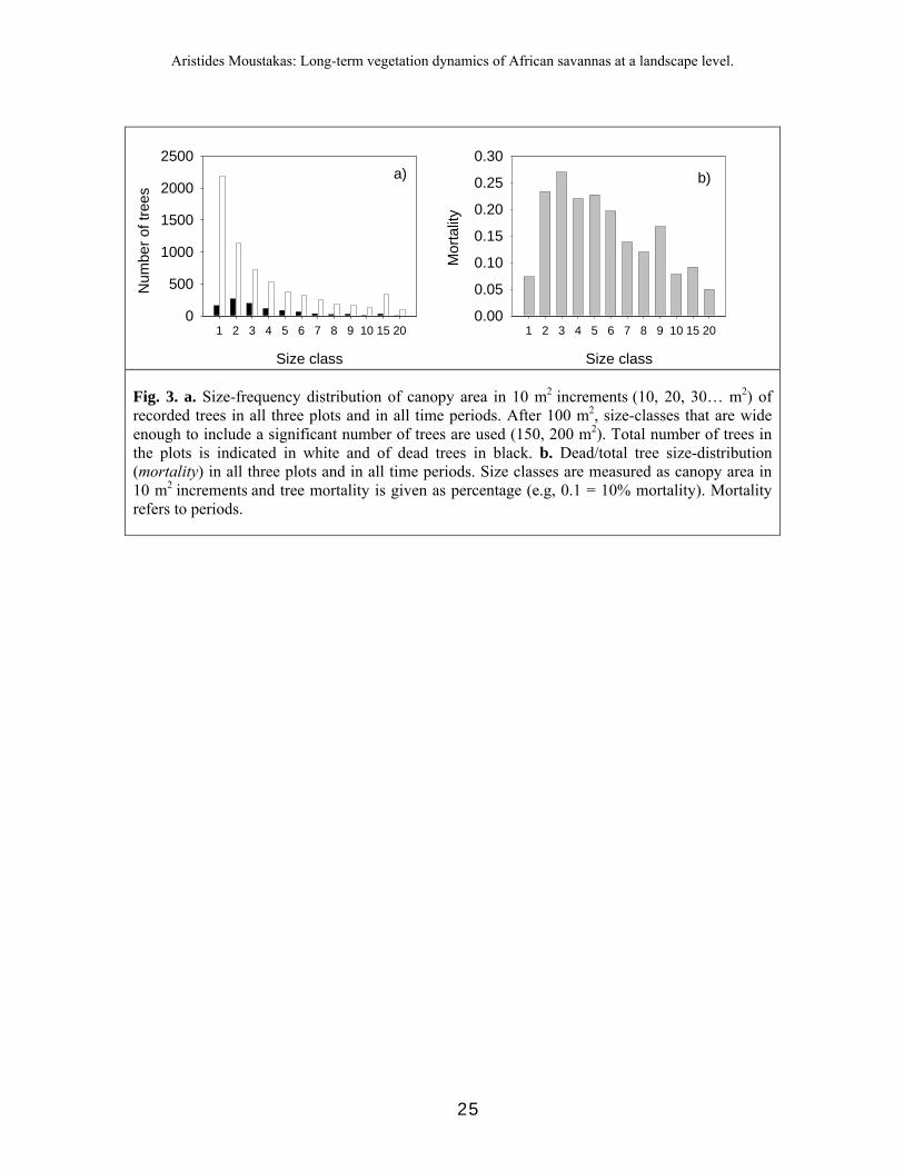
Fig. 3. a. Size-frequency distribution of canopy area in 10 m2 increments (10, 20, 30… m2) of recorded trees in all three plots and in all time periods. After 100 m2, size-classes that are wide enough to include a significant number of trees are used (150, 200 m2). Total number of trees in the plots is indicated in white and of dead trees in black. b. Dead/total tree size-distribution (mortality) in all three plots and in all time periods. Size classes are measured as canopy area in 10 m2 increments and tree mortality is given as percentage (e.g, 0.1 = 10% mortality). Mortality refers to periods.
25

Aristides Moustakas: Long-term vegetation dynamics of African savannas at a landscape level.
Year 1940 1964 1984 1993 2001 Plot 1 Total tree cover (m2) 11692 10774 11262 12656 13670 Relative tree cover [%] 0.78 0.72 0.75 0.84 0.91 Total trees 370 230 325 361 526 Mean tree size (m2) S.D.
31.60 28.32
46.85 36.91
34.66 38.19
35.06 39.25
25.99 32.71
Dead trees 74 25 14 29 Mean annual death rate (%) 0.93 0.57 0.49 1.04 Plot 2 Total tree cover (m2) 6964 13845 21322 22951 Relative tree cover [%] 0.42 0.84 1.30 1.39 Total trees 488 853 814 1027 Mean tree size (m2) S.D.
14.27 19.15
16.23 20.75
28.35 33.38
22.35 23.82
Dead trees 99 54 74 Mean annual death rate (%) 1.13 0.72 1.18 Plot 3 Total tree cover (m2) 18834 27767 52248 39883 26902 Relative tree cover [%] 0.95 1.40 2.65 2.02 1.36 Total trees 621 691 1078 855 817 Mean tree size (m2) S.D.
30.32 30.53
40.18 39.60
48.67 58.53
55.16 57.44
32.93 39.84
Dead trees 80 35 253 60 Mean annual death rate (%) 0.57 0.26 2.93 0.91
Table 1. Tree characteristics for each different plot and period. For each plot and for each period (year) we list total area covered by tree canopies (Total tree cover in m2), the relative area covered by tree canopies (Relative tree cover in %), the total number of trees (Total trees), the mean and standard deviation of canopy area of total trees (Mean tree size in m2 and S.D.), the number of dead trees (Dead trees), and the percentage of mean annual death rate (according to eq. 1). Dead trees refer to the interval, namely the 1940 death rate derives from the dead trees between 1940-1964. The other statistics refer to the year the picture was taken. So we always refer back to the last time that the dead trees were seen. In plot 1 during 1940-1964, 89 trees were cut by the farm manager.
26

Aristides Moustakas: Long-term vegetation dynamics of African savannas at a landscape level.
Year 1940 1964 1984 1993 2001
Plot 1 dead total dead total dead total dead total total
1940 dead 1 0.127
(0.462) 0.299
(0.385) 0.127
(0.462) 0.588
(0.308)
total 1 0.588
(0.308) 0.999
(0.154) 0.999
(0.154) 0.999
(0.154)
1964 dead 1 < 0.001** (0.769)
0.898 (0.231)
0.999 (0.077)
total 1 0.999
(0.154) 0.897
(0.231) 0.588
(0.301)
1984 dead 1 < 0.001** (0.846)
0.897 (0.231)
total 1 0.999
(0.154) 0.999
(0.154)
1993 dead 1 0.003* (0.692)
total 1 0.999
(0.154) Plot 2
1964 1984 1993 2001 dead total Dead total dead total total
1964 dead 1 0.898
(0.231) 0.999
(0.154) 0.898
(0.231)
total 1 0.588
(0.308) 0.127
(0.462) 0.299
(0.385)
1984 dead 1 0.045
(0.539) 0.898
(0.231)
total 1 0.299
(0.385) 0.898
(0.238)
1993 dead 1 0.013
(0.615)
total 1 0.999
(0.154) Plot 3
1940 1964 1984 1993 2001 dead total dead total Dead total dead total total
1940 dead 1 0.003* (0.692)
0.999 (0.154)
0.898 (0.231)
0.999 (0.154)
total 1 0.588
(0.308) 0.044
(0.539) 0.126
(0.462) 0.588
(0.308)
1964 dead 1 < 0.001** (0.923)
0.588 (0.308)
0.588 (0.308)
total 1 0.588
(0.308) 0.898
(0.231) 0.898
(0.231)
1984 dead 1 < 0.001** (0.769)
0.588 (0.308)
total 1 0.898
(0.231) 0.588
(0.308)
1993 dead 1 < 0.001** (0.923)
total 1 0.588
(0.308) App. 1. Comparisons of tree size-class distributions (dead vs. dead, dead vs. total, and total vs. total) on each plot and time period. Kolmogorov-Smirnov tests were used and P and (Dmax) values are listed. In each time period, trees are divided into total trees present on the plot and dead trees. Mortality refers to an interval, namely the 1940 mortality are the dead trees between 1940-1964. So we always refer back to the last time that the dead trees were seen. Dead trees are included in the number of total trees. P values are calculated with Bonferroni adjustments for multiple comparisons.
27

Aristides Moustakas: Long-term vegetation dynamics of African savannas at a landscape level.
CHAPTER 3: The paradox of climate-dependent growth in one of the world’s deepest-rooted trees, Acacia erioloba
Aristides Moustakas1*, Christoph Scherber1, KerstinWiegand1, David Ward3, MatthiasGuenther2, Karl-Heinz Mueller2
1Institute of Ecology, Friedrich Schiller University, Dornburgerstr. 159, 07743 Jena, Germany 2 Department of Geography , Research Lab GIS & Remote-sensing, Philipps University Marburg, Deutschhausstr. 10, 35037 Marburg, Germany 3School of Biological & Conservation Sciences, University of KwaZulu-Natal, P. Bag X1, Scottsville 3209, South Africa This chapter will be submitted to Plant Ecology Abstract We investigated long-term growth of Acacia erioloba, a long-lived and deep-rooted tree, in a South African savanna (Kalahari) using remote-sensing techniques. Our remote-sensing techniques comprise of processed aerial photographs taken in 1940, 1964, 1984, and 1993. We used isolated individuals exclusively, in order to exclude intraspecific competition effects from our analysis. Our study areas were virtually free of fire, browsing, and disease. Our results show that individual trees do not necessarily grow over long time intervals, even though overall the tree population had a positive size increment. Tree growth was size-independent. There was also a interval where mean tree increment was negative. Growth was mainly influenced by precipitation in combination with high summer temperatures. Paradoxically, we found that total aboveground green biomass was related to rainfall fluctuations despite A. erioloba being one of the deepest-rooted trees in the world. These results indicate that access to groundwater does not necessarily preclude the influence of annual rainfall on productivity of trees. Keywords: tree growth, long term data, remote-sensing, savanna, size independent growth, tree size, climate. Introduction
An understanding of size-age relationships and age or size-specific growth is the basis
for understanding and predicting vegetation change in assemblages of long-lived plants, whether the management objectives are conservation of biodiversity or agricultural production (Wiegand T. et al. 2000). However, long-term data on growth and mortality are scarce due to the difficulties involved in collecting them. This problem is particularly acute in the case of long-lived trees, whose lifetimes are usually considerably longer than those of researchers. Moreover, there is a scientific bias towards the study of northern hemisphere versus southern hemisphere plants.
28

Aristides Moustakas: Long-term vegetation dynamics of African savannas at a landscape level.
It is generally assumed that there is a relationship between tree age, size, and growth (White and Harper 1970) as well as between tree age, size, density, and disturbance (Niklas et al. 2003; Coomes et al. 2003). However, size and age are not necessarily strongly correlated. For many organisms birth, growth and death may depend more upon the size than the age of individuals (Harper 1977). The most common assumption in estimating tree age is that the largest trees are likely to be old (Harper 1977). Savanna tree life cycles are known to be long but are unquantified (Midgley and Bond 2001). Age estimation of Acacia trees is not possible using tree rings because they may have several rings in wet years and none in dry years (Gourlay 1991). In A. erioloba, tree rings may reveal time since release from fire or browsing rather than age (Gourlay 1995). Due to the longevity of Acacia species and the absence of long-term data, simulations were carried out to estimate the relationship among age/size and growth and mortality on Acacia species but no clear relationship was found (Wiegand et al. 2000b). Due to the absence of long-term data for savanna tree growth, a common approach is to apply a constant growth function (e.g. Wiegand et al. 1999; Fox et al. 2001).
Savannas cover about 13% of the global land surface and about half of the area of Africa, Australia and South America (Scholes and Archer 1997). Trees in the savanna are critical for providing shade and shelter to animals (Belsky et al. 1989; Belsky 1994), and they influence plant communities by altering soil moisture and nutrient concentration (Belsky et al. 1989). Tree cover in arid woodlands is lower than tree cover in mesic or humid woodlands; therefore land use of arid woodlands is more prone to desertification (Shepherd 1991). In general, arid and semi-arid ecosystems are less managed than northern hemisphere hardwoods, and therefore more natural (Gourlay 1995). Acacia erioloba is a keystone tree species in the Kalahari Desert and in African savannas (Milton and Dean 1995). It is an appropriate species to carry out a long term study on tree growth because it is a long-lived tree (Barnes et at. 1997). The fact that individuals of this species have very deep roots allowing them access to permanent groundwater sources (Jennings 1974) makes A. erioloba less affected to climatic variations than other trees (Barnes et al. 1997).
Unlike forests where light is a primary limiting resource, savanna tree growth is mainly limited by nutrients and water (Frost et al. 1986; Coomes and Grubb 2000), so we expect forest species to allocate more resources aboveground to light capture and savanna species to capture of below-ground resources (Coomes and Grubb 2000, Hoffmann and Franco 2003). Savannas are more stressful and unproductive environments than forests and thus savanna trees grow slower (Grime 1977; Chapin et al. 1993). Good studies on savanna tree growth have been conducted (e.g. Miller et al. 2001; Shackleton 2002; Hoffmann and Franco 2003). However, most of them are relative short-term studies covering up to 10 y time. In a long-term study of growth rings in a tropical semi-deciduous forest, it was found that annual growth rings are related to precipitation patterns (Worbes 1999). There are no studies on long-term savanna tree growth to our knowledge.
Given the absence of long term data on African savanna trees, we used aerial photographs covering 53 y to provide us with long-term spatial data on tree size that are necessary to quantify tree growth. We have aerial photographs of the study area from 1940, 1964, 1984 and 1993. In this paper we study the growth of A. erioloba individuals that are isolated (minimum distance to nearest neighbour was 25 m) and therefore their
29
Aristides Moustakas: Long-term vegetation dynamics of African savannas at a landscape level.
growth is largely independent of intra-specific competition (Coomes et al. 2002). The growth of these trees is not influenced by inter-specific competition because our study plots contain A. erioloba trees exclusively.
Using the data extracted by these methods, we sought to quantify the relationship between size and growth of A. erioloba through time. Furthermore, we analyzed climatic parameters and tried to detect a relationship between climate and tree growth.
Study area and Methods
Information and history of the study area
Our two study plots are located on Dronfield Ranch, near Kimberley, Kalahari, South Africa. Both plots are rectangular and their locations are: Plot 1, 28o 38´ 43´´ S and 24o 51´ 19´´ E, Plot 2, 28o 37´ 48´´ S and 24o 50´ 7´´ E. Rain mainly falls during summer months, namely December - February. Mean annual precipitation is 411 mm per year, summer mean maximum daily temperature is 32 oC, and winter mean minimum daily temperature is 3.3 oC (data from South African Weather Forecast Service). In all plots, soil consisted of mainly Hutton (haplic arenosol) soil type and was > 2 m deep (S. African Dept. of Agric. Tech. Serv. 1974, and soil samples taken by us in the field, unpublished data).
The land was bought by the De Beers Consolidated Mines Ltd. in 1870 to serve as rangeland for horses, donkeys, and oxen used as draft animals in the diamond mines of Kimberley. Initially, the ranch was managed with cattle and wild mammalian herbivores. The game was gradually removed from the land and cattle were ranched for a interval. In the past year, the cattle have been removed and it has been converted into a game ranch.
In our two study plots, A. erioloba is the only tree species present. Cattle do not browse A. erioloba but game does (Barnes 2001). Therefore, there was little browsing of A. erioloba. There were no tree diseases or tree pruning in our plots. In the area there is groundwater which is pumped using windmills. Fire is not a common event in our study area because there is insufficient grass fuel to support a large fire (A. Anthony, pers. comm.).
A. erioloba characteristics
A. erioloba is generally drought resistant (Barnes et al. 1997). This is possible because A. erioloba is a deep-rooted tree allowing them access to deep groundwater sources. A. erioloba is one of the deepest rooted trees in the world: Jennings (1974) recorded A. erioloba roots at 68 m, while Story (1958) found roots down to 45 m. It occurs in deep sands where it is usually the dominant tree and it is generally assumed that they are dominant because they are able to access the deep aquifers (Barnes et al. 1997). In adjacent habitats where sands are shallow or where the aquifers are close to the surface, A. erioloba is outcompeted by A. mellifera, A. tortilis and Tarchonanthus camphorates (D. Ward pers. observ.). Even though in arid environments trees are usually deep-rooted (Schenk and Jackson 2002), A. erioloba is a very deep-rooted tree (Barnes et al. 1997; Robertson 2005). It generally lives very long and cases of trees older than 250 y have been recorded (Timberlake 1980).
30
Aristides Moustakas: Long-term vegetation dynamics of African savannas at a landscape level.
Remote-sensing Methods
For the identification and multi-temporal analysis of A. erioloba we used black-and-white aerial photographs of the area taken in 1940, 1964, 1984, and 1993, and an Ikonos satellite image taken in 2001. We were able to identify and follow every individual tree from 1940 to the next available photo till 2001. Our classification accuracy was 1 m. We therefore decided to include trees with canopy surface of at least 2 m to ensure high classification reliability. Ground-truth field work was also carried out for verification. For further details concerning the remote-sensing methods see Moustakas et al. (in press). Data classification
Using the remote-sensing techniques described above, we identified tree individuals on each of the 2 plots during years 1940, 1964, 1984, 1993 and 2001. In each plot, and for each year, we numbered each tree vector and we extracted its tree size in terms of canopy area (projection area) in m2 and its center coordinates using MapInfo Professional 7.0. We tracked the trees through time starting from 1940. If a tree did not appear in the database of the plot in the next time step, we assumed that this tree had died within the time interval considered. For verification, for each tree that did not appear in the next database, we searched near its center (i.e. where it appeared the last time that the tree was detected), in the next database. Statistical power for analyses of trees that survived until 2001 was too small (5 trees); we therefore excluded the 2001 data from our analyses. Results on nearest tree neighbourhood analysis and tree pattern analysis, showed that in our study area the zone of influence was maximum 25 m (Moustakas et al. unpublished analysis). This means that the in our plots, the risk of death due to inter-tree competition is significant for trees distancing up to 25 m and almost negligible at > 25 m distances. In this paper we include trees that their nearest tree neighbour is at least 25 m away (i.e. “isolated” trees). Thus, our analyses comprise isolated trees that were firstly seen at 1940 and survived until 1993. Trees that were first seen in 1940 but died before 1993 were also excluded from the analyses. This resulted in 43 identified trees that survived from 1940 until 1993.
Allometry of A. erioloba
Given that there is no standard index for describing tree size, we measured the size of 29 A. erioloba trees in terms of height, stem circumference, and canopy area. To facilitate the conversion between these three common indices, we determined allometric relationships among these characteristics via linear regression.
Statistical analyses
Given that we selected isolated trees, we minimized the effect of competition. Thus, climate should be the most important factor influencing tree growth in our study. We chose three climatic variables: mean annual precipitation, mean daily summer temperature maxima (hereafter referred to as mean max temperature), and mean daily winter temperatures minima (mean min temperature). To determine mean max
31
Aristides Moustakas: Long-term vegetation dynamics of African savannas at a landscape level.
temperature for a given year, we calculated the mean daily summer temperature maximum, i.e. the mean over daily maximum temperatures during the summer months December, January, and February. Note that tropical savannas are summer rainfall areas. Mean max temperature was chosen because summer temperatures of summer rainfall areas are directly related to the amount of water loss due to evapotranspiration (Wiegand T et al. 2004). Mean min temperature of a given year is the mean of the daily recorded minimum temperatures during June, July, and August. Mean min temperature is relevant because of possible negative effects of frost on tree growth.
As a first step regarding the influence of climate on tree growth, we searched for patterns in the three climatic indices. To detect possible climatic cycles, we applied autocorrelation analysis. The autocorrelation function (ACF) which is the Pearson product-moment correlation between any point Y(t) along a time series, and the corresponding Y(t+k) at time step k, where k ∈ {0,1,2,3, ...}. We used ACF to detect non-randomness in the climate data of interest, i.e. whether there were linear trends or cyclical patterns.
We used analyses of variance (ANOVA) to test for differences between climate variables at different time intervals, where the following intervals were treated as categorical explanatory variables: 1932-1939, 1940-1963, 1964-1983, 1984-1993, and 1994-2001. Even though we had no tree data during 1932-1939 and 1994-2001, climatic analysis was carried out during these intervals too as it provided us with a better overview over climatic trends. In cases where model outputs showed significant effects of time interval, we used orthogonal contrast coefficients to test which levels of the factor “time interval” were significantly different from one another (Crawley 2002). As there were five different intervals, the contrast coefficient matrix had four columns. The intervals tested were (i) interval 1 vs. interval 2; (ii) interval 1 vs. interval 3; (iii) interval 3 vs. interval 4 and (iv) interval 2 vs. interval 5.
We used paired t-tests to examine if tree growth during a given time interval (starting with 1940-1963) was correlated with tree size in the sequential time interval. To quantify average growth (independent of climate), we applied linear least-squares regression between growth and time analysis to all years and trees. Based on these results, we determined time-dependent growth of A. erioloba. For each interval, this iterative growth function has the form:
),()()( tigtitimts ×
Δ−
+= (A)
where i and t are the initial and final year of each time interval tΔ = t-i, s(t) is the tree size at time t, m(i) is the mean size of all trees at time i, and ),( tig is the average growth of all trees during the time interval . All time variables are measured in years and all size and growth variables in m
tΔ2 canopy area. Given that we have 4 available photos, we
parameterized the growth function for each of the three successive intervals. We also extrapolated the growth of the interval 1940-1964 backwards in order to estimate the year during which a tree with average growth germinated. In the absence of more complete data, this estimate is based on the assumption that growth before 1940 and during 1940-1964 was equal.
32

Aristides Moustakas: Long-term vegetation dynamics of African savannas at a landscape level.
Results
We found tight allometric relationships between height, stem circumference, and canopy area of A. erioloba (all R2 about 0.9 and all P<0.001; Fig. 1).
Examining the mean annual precipitation data, it is clear that variation is high (min=177 mm, max=802 mm, St. Dev.=132 mm; Fig. 2a). Analyses of Variance (ANOVA) on the amount of rainfall within the 5 time intervals showed no significant difference among any of the intervals (ANOVA: F =0.611, P=0.656, df=4). However, autocorrelation analysis of rainfall showed that there was a significant negative autocorrelation every 10 years and a significant positive autocorrelation every 14 years (Fig. 3a). In other words, if a given year is arid, then we expect a wet year after 10 years and another arid year after 14 years. Given that our photos were taken at intervals that of 9 to 24 years, a dry and a wet year is expected to have occurred within each photo interval.
Analysis of mean max temperatures through years showed also high variability (min=28.8oC, max=38.7oC, St. Dev=1.4oC; Fig 3b). An extremely hot summer took place in 1992 with average maximum daily temperatures over 39oC. There was no significant difference in mean max temperature among any of the 5 time intervals (ANOVA: F =1.03, P=0.4, df=4). Autocorrelation analysis showed no periodicity in mean max temperatures (Fig. 3b).
Results concerning mean min temperatures, showed also variability in time (min=0.9oC, max=5.2oC, St. Dev=1.1oC; Fig. 2c). However, there were significant differences among the time intervals except interval 2 vs. 5 where differences were non-significant (Table 2). Overall, mean min temperatures among time intervals differed significantly (ANOVA: F=7.442, P<0.001, df=4). Visual inspection of Fig. 2c shows that these differences may be due to a long-term cycle with a period (in the trigonometrical sense) comparable to our study duration, which can thus not be picked up by autocorrelation analysis. However, autocorrelation analysis did detect 4-year cycles of mean min temperatures (Fig. 3c). Therefore, 4 mild winters were followed by 4 colder ones, meaning that all photo intervals included both cold and warmer winter intervals.
Most trees were larger in 1964 than in 1940 (Fig. 4a). During 1984, only four trees were smaller than their initial size during 1940 (Fig. 4b). However, several trees were smaller in 1993 than in 1940 (Fig. 4c). Paired t-tests showed that initial tree size had no effect on tree growth. An exception to this is the interval 1984-1993, where growth increment was negatively correlated with tree size in 1984 (t=-2.179, p=0.035, df=41), mainly due to dieback of large trees (Fig. 4c). Overall, there was positive tree growth during 1940-1964 (Fig. 4d); even higher mean tree growth was recorded in 1964-1984 (Fig. 4e). Although some tree individuals grew between 1984-1993, most trees were smaller than they were in 1984 (Fig. 4f).
Examining size of individual trees relative to their size in 1940, it is clear that most trees were larger in 1964 (Fig. 4a; 4d). Only 4 trees were smaller or slightly smaller than their initial size during 1984 (Fig. 4b; 4e). However, several trees were smaller in 1993 than in 1940 (Fig. 4c; 4f). Paired t-tests showed that initial tree size had no effects on tree growth except during the interval 1984-1993, where growth increment was negatively
33

Aristides Moustakas: Long-term vegetation dynamics of African savannas at a landscape level.
correlated to tree size in 1984 (t=-2.1795, df=41, p=0.035). Thus tree growth was not correlated with initial tree size.
The iterative equations that describe tree size with time as an independent variable are:
1940-1964 (A1): 16.2024194032.47)( ×
−+=
tts
1964-1984 (A2): 33.3120196448.67)( ×
−+=
tts
1984-1993 (A3): )27.9(9198481.98)( −×
−+=
tts
Applying (A1) backwards and solving s(t) = 0, gives t=1883. Therefore, an average/typical tree germinated around 1883 (Fig. 5), had a canopy area of 47.3 m2 in 1940 (Table 1) and was therefore about 110 years old in 1993. Overall, maximum tree growth was recorded in the 1964-1984 interval (Fig. 5). Tree increment was negative during the 1984-1993 interval.
In order to provide an estimate of the age of a tree of size y that one can observe in the field, we used the average growth and St.Dev. of the 1940-64 interval (Table 1), during which growth was intermediate, to plot an average size-age relationship and 95% confidence interval. Age (A) is calculated in years meanwhile tree size (S) is the canopy area in m2. A = a × S + b, where a=1.3, b=-4.7 and the 95% confidence interval of a = [0.93, 2.08]. Therefore:
A ≈ 1.3 × S − 4.7 (B) Even though eq. (B) is calculated over a interval were a positive growth took place, negative growth is possible too. Negative growth increment is feasible too as observed during the 1984-1993 interval.
34

Aristides Moustakas: Long-term vegetation dynamics of African savannas at a landscape level.
Max. canopy diameter (m)
0 5 10 15 20 25
Hei
ght (
m)
0
2
4
6
8
10
y = 0.291x + 2.59
R2 = 0.85, P<0.001
Stem circumference (cm)
0 50 100 150 200 250 300
Max
. can
opy
diam
eter
(m)
0
5
10
15
20
25
y = 0.077x + 0.31
R2 = 0.91, P<0.001
Stem circumference (cm)
0 50 100 150 200 250 300
Hei
ght (
m)
0
2
4
6
8
10
y = 0.023x + 2.63
R2 = 0.86, P<0.001
Figure 1. Allometric and linear regression relationships of A. Erioloba characteristics.
35
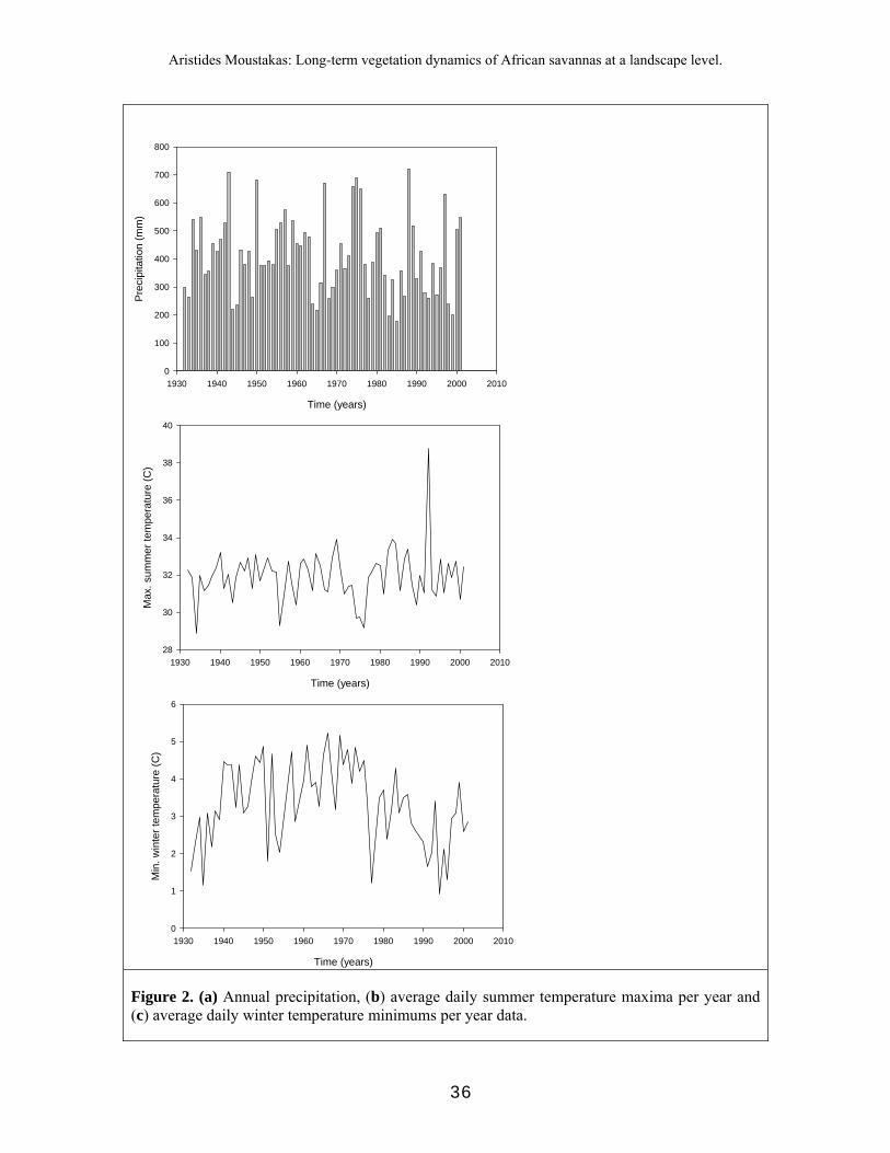
Aristides Moustakas: Long-term vegetation dynamics of African savannas at a landscape level.
Time (years)
1930 1940 1950 1960 1970 1980 1990 2000 2010
Prec
ipita
tion
(mm
)
0
100
200
300
400
500
600
700
800
Time (years)
1930 1940 1950 1960 1970 1980 1990 2000 2010
Min
. win
ter t
empe
ratu
re (C
)
0
1
2
3
4
5
6
Time (years)
1930 1940 1950 1960 1970 1980 1990 2000 2010
Max
. sum
mer
tem
pera
ture
(C)
28
30
32
34
36
38
40
Figure 2. (a) Annual precipitation, (b) average daily summer temperature maxima per year and (c) average daily winter temperature minimums per year data.
36

Aristides Moustakas: Long-term vegetation dynamics of African savannas at a landscape level.
)(igYear Δt (years) m(i) (m2) St. Dev. (m2) (m2)
1940 47.3 1964 24 67.5 25.78 20.2 1984 20 98.8 36.64 31.3 1993 9 89.6 29.59 -9.3
Table 1. Mean tree size [(m(i)] in terms of canopy area, mean growth increment [ )(ig ], and standard deviation of growth increment [St. Dev.] of the 41 studied trees. Mean growth and St. Dev. were averaged over each two sequential available photos.
Interval F P df 1 vs. 2 13.237 <0.001** 1 1 vs. 3 9.115 0.004** 1 3 vs. 4 4.227 0.04* 1 2 vs. 5 3.188 0.079 1
Table 2. ANOVA tests of mean daily winter temperatures minima.
37

Aristides Moustakas: Long-term vegetation dynamics of African savannas at a landscape level.
0 5 10 15
-0.2
0.0
0.2
0.4
0.6
0.8
1.0
Time Lag (years)
Auto
corr
elat
ion
Func
tion
Average precipitation per year
0 5 10 15
-0.2
0.0
0.2
0.4
0.6
0.8
1.0
Time Lag (years)
Auto
corr
elat
ion
Func
tion
Average daily summer temperature maxima per year
0 5 10 15
-0.2
0.0
0.2
0.4
0.6
0.8
1.0
Time Lag (years)
Auto
corr
elat
ion
Func
tion
Average daily winter temperature minima per year
Figure 3. Autocorrelation analysis of (a) annual precipitation, (b) average daily summer temperature maxima per year and (c) average daily winter temperature minima per year data. The dotted lines indicate the level of significant differences.
38
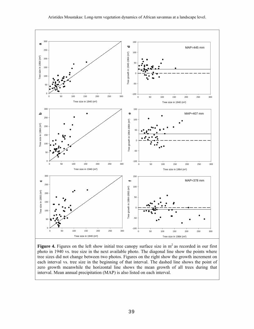
Aristides Moustakas: Long-term vegetation dynamics of African savannas at a landscape level.
Tree size in 1940 (m²)
0 50 100 150 200 250 300
Tree
siz
e in
196
4 (m
²)
0
50
100
150
200
250
300
Tree size in 1940 (m²)
0 50 100 150 200 250 300
Tree
siz
e in
198
4 (m
²)
0
50
100
150
200
250
300
Tree size in 1940 (m²)
0 50 100 150 200 250 300
Tree
siz
e in
199
3 (m
²)
0
50
100
150
200
250
300
Tree size in 1984 (m²)
0 50 100 150 200 250 300
Tree
gro
wth
in 1
984-
1993
(m²)
-100
-50
0
50
100
150
Tree size in 1964 (m²)
0 50 100 150 200 250 300
Tree
gro
wth
in 1
964-
1984
(m²)
-100
-50
0
50
100
150
Tree size in 1940 (m²)
0 50 100 150 200 250 300
Tree
gro
wth
in 1
940-
1964
(m²)
-100
-50
0
50
100
150
MAP=407 mm
MAP=445 mm
MAP=378 mm
ab
c
de
f
Figure 4. Figures on the left show initial tree canopy surface size in m2 as recorded in our first photo in 1940 vs. tree size in the next available photo. The diagonal line show the points where tree sizes did not change between two photos. Figures on the right show the growth increment on each interval vs. tree size in the beginning of that interval. The dashed line shows the point of zero growth meanwhile the horizontal line shows the mean growth of all trees during that interval. Mean annual precipitation (MAP) is also listed on each interval.
39

Aristides Moustakas: Long-term vegetation dynamics of African savannas at a landscape level.
Time (years)
1880 1890 1900 1910 1920 1930 1940 1950 1960 1970 1980 1990 2000
Tree
siz
e (m
2 )
0
20
40
60
80
100
120
Figure 5. Mean tree size as a (linear) function of time in each interval according to eq. A1, A2, A3. The dashed line is a backwards linear extrapolation of eq. A1 in order to estimate the year that the trees germinated. Discussion
Given that aerial photographs are black-and-white, seasonal fluctuations in total
aboveground green biomass (which varies seasonally) do not influence the classification of tree size. Furthermore, in the study area there is little game, therefore, browsing of A. erioloba trees with canopy diameter of at least two m, which are included in this paper, is negligible. Therefore differences in tree size on different photos are not due to such effects. Size-growth-age relationship
Overall, A. erioloba growth is not size-dependent according to our results. Wiegand et al. (2000b) found that “growth increment is only weakly correlated with tree size” in A. raddiana. However, in the abovementioned study, growth was measured in terms of trunk circumference meanwhile we investigated growth in terms of canopy area. In another study in a similar environment, size-independent growth (in terms of canopy
40

Aristides Moustakas: Long-term vegetation dynamics of African savannas at a landscape level.
area) was also recorded for some of the species investigated. (Wiegand T. et al. 2000). However none of the investigated species were Acacias. Therefore we cannot infer that A. erioloba growth is generally size-independent because whether growth is size dependent or not could depend on the measurement used or species identity.
We observed both negative and positive growth. This seems to be a common feature of Acacia trees because the same phenomenon has been observed for A. raddiana trunks in the Negev desert of Israel (Wiegand et al. 2000) and A. reficiens canopies in a savanna in Namibia (Wiegand et al. 2005). It seems that most of the time growth is size-independent but in extremely dry/hot years the bigger trees shrink most.
We calculated that the 43 trees investigated by us were approximately 110 y old in 1993. Given that A. erioloba are considered to live well beyond 200 y (Timberlake 1980, Barnes et al. 1997), these trees were not expected to die in the near future due to ageing. Therefore, factors other than current tree size affect tree growth. Even though the 53 y interval that our photos cover comprises only about a fifth of A. erioloba life span, no obvious relationship between growth and age can be derived. Trees during 1984-1993, which are on average about 100 y old, have on average a negative increment. However trees in 1940-1964 that were about 60-80 grew slower than in 1964-1984 that were about 80-100 y old. Thus, there is a lot of variation on long-term A. erioloba growth.
We estimated that the trees in our plots germinated around 1883. Interestingly, diamonds were discovered in Kimberley in 1867 (Beet 1914). During that year, most of the trees in the area were eliminated for the mines. Since in the area of the Dronfield ranch no diamonds were found, the land was used to serve as rangeland for horses, donkeys, and oxen used as draft animals in the places that diamond were found. Therefore after the elimination of trees in 1867, trees germinated again in Dronfield. Given that tree germination in semi-arid savannas is a rare episodic event that can easily take 15 y to take place (van Rooyen et al. 1984), it seems realistic that trees germinated around 1883.
Given the long Acacia life cycles and the absence of long-term data, management decisions are mainly taken with the assistance of models (e.g. Burrows et al. 1990). However, in order to lead to reliable results models need to be based on data. Thus, a number of published field studies are needed for realistic model calibration. Long-term A. erioloba growth (over 100 y) could be approximated with a linear growth function for building models as done by Wiegand et al. 1999 and Fox et al. 2001. However, growth variation is high and party explained by climatic factors.
Additionally, there is evidence that increasing levels of global CO2 favor the growth of trees which are C3 species rather than grasses which are mainly C4 species (Knapp 1993). Under higher CO2 levels, net photosynthetic efficiency of C3 species will increase faster than in C4 species (Wolfe and Erickson 1993). However, it is not known if CO2 has increased enough to cause such change (Wolfe and Erickson 1993) and absence of long-term data on past tree growth prevents us from detecting such possible influences. However the average decrease of tree size in the last growth interval doesn’t seem to indicate such a positive effect of CO2 on growth.
41

Aristides Moustakas: Long-term vegetation dynamics of African savannas at a landscape level.
Role of climate
According to our analysis, precipitation extremes follow 10 y cycles and winter low temperatures follow 4 y cycles. The time intervals between our photos range from 9 - 24 y. Therefore, in each interval, there are on average at least 2 extreme climatic phenomena included. However, mean summer maximum temperatures and mean annual precipitation were not different in each interval. Therefore, the reasons that could explain the derived growth function and the different growth rates in each interval should come from extreme events rather than mean properties. Combining the results of climate (Fig. 2) and overall growth (Fig. 5), one can see that during 1940-1964 there were fairly mild winters and not very hot summers. However there were few above average wet years in a row. During 1964-1984, where growth was the maximum recorded, summers were fairly mild, there was an extremely cold winter but there were also three sequentially wet years. These wet years were combined with mild summers. Taking into account that the rainy season is almost exclusively during summer months, a high percentage of the rain that falls during warm days is lost due to evapotranspiration (Wiegand T et al. 2004). During the wet years of 1974-1976, summer temperatures were fairly mild. Therefore the amount of water that penetrated the soil was high. During 1984-1993, there were two sequential fairly wet years in 2000-2001 combined with normal summer temperatures; however there was an extremely warm summer in 1992 with below average precipitation as well. Given that A. erioloba growth occurs from November to March (Barnes et al. 1996), cold winter temperatures do not seem to be influential. Given that A. erioloba is one of the deepest rooted trees in the world, it appears that it can create a buffer against climatic uncertainty by gaining access to deep water. However, growth is influenced by climatic extremes. Therefore, key factors for A. erioloba growth in our study were precipitation in combination and summer temperature maxima.
Short-term studies on arid savanna tree growth show that precipitation is the key factor (Miller et al. 2001, Shackleton 2002). A study on Acacia growth ring characteristics also found that the key factor explaining the formation of growth rings was precipitation (Gourlay 1995). However, in none of the abovementioned studies was ambient temperature included in the analysis. In addition, in the abovementioned studies, growth analysis did not exceed a 10 y time interval. In a review of tree growth models the importance of temperature on tree growth is highlighted (Schenk 1996).
Even though it is well cited that A. erioloba is a very deep-rooted tree (Story 1958; Jennings 1974; Barnes et al. 1997) it is possible that the individuals in this study did not actually have access to ground water. However this is very unlikely. Soil in our study area is sandy and > 2 m. In addition, there are no other trees present. Ground water exists on the area and it is pumped with wind mills. Thus, in spite of the fact that A. erioloba is able to access deep water sources, growth is clearly related to precipitation. This leads to the paradox that growth in one of the deepest-rooted trees in the world is affected by climatic fluctuations. These results indicate that access to aquifers is a buffer (albeit not a particularly effective one) against dry intervals but does not provide the primary source of water for these trees, at least for aboveground growth.
42
Aristides Moustakas: Long-term vegetation dynamics of African savannas at a landscape level.
References
Anonymous. (1974). Land type survey. Department of Agricultural Technical Services.
Pretoria. Barnes, M.E. (2001). Seed predation, germination and seedling establishment of Acacia
erioloba in northern Botswana. Journal of Arid Environments, 49: 541-554. Barnes, R.D., Fagg, C.W., Milton, S.J. (1997). Acacia erioloba. Monograph and
annotated bibliography. Oxford Forestry Institute, Department of Plant Sciences, University of Oxford.
Barnes, R.D., Marunda, C.T., Makoni, O., Maruzane, D., Chimbalanga, J. (1996). African Acacias: Genetic evaluation: Phase I. Final Report of ODA Forestry Research Scheme R5653. Oxford Forestry Institute and Zimbabwe Forestry Commission.
Beet, A.J. (1914). Kimberley: Its history and diamonds, Kimberley, South Africa. Belsky, A.J. (1994). Influences of trees on savanna productivity: tests of shade, nutrients,
and tree-grass competition. Ecology, 75: 922-932. Belsky, A.J., Amundson, R.G., Duxbury, J.M., Riha, S.J., Ali, A.R., Mwonga, S.M.
(1989). The effects of trees on their physical, chemical, and biological environment in a semi-arid savanna in Kenya. Journal of Applied Ecology, 26: 1005-1024.
Burrows, W.H., Carter, J.O., Scanlan, J.C., Anderson, E.R. (1990). Management of savannas for livestock production in north-east Australia: contrasts across the tree-grass continuum. Journal of Biogeography, 17: 503-512
Chapin, F.S., Autumn, K., Pugnaire, F. (1993). Evolution of suites of traits in response to environmental stress. American Naturalist (Suppl.), 142: S78–S92.
Coomes, D.A., Duncan, R.P., Allen, R.B., Truscott, J. (2003). Disturbances prevent stem size-density distributions in natural forests from following scaling relationships. Ecology Letters, 6: 980-989.
Coomes, D.A., Grubb, P.J. (2000). Impacts of root competition in forests and woodlands: A theoretical framework and review of experiments. Ecological Monographs, 70: 171-207.
Coomes, D.A., Rees, M., Turnbull, L., Ratcliffe, S. (2002). On the mechanisms of coexistence among annual-plant species, using neighborhood techniques and simulation models. Plant Ecology, 163: 23-38.
Crawley, M.J. (2002). Statistical Computing: An Introduction to Data Analysis using S-Plus. Wiley. Fox, J.C., Ades, P.K., Bi, H.Q. (2001). Stochastic structure and individual-tree growth
models. Forest Ecology and Management, 154: 261-276. Frost, P., Medina, E., Menaut, J.-C., Solbrig, O., Swift, M., Walker, B. (1986). Responses
of savannas to stress and disturbance. Biology International, Special Issue, 10: 1–82. Gourlay, I.D. (1995). Growth ring characteristics of some African Acacia species. Journal
of Tropical Ecology, 11: 121-140. Gourlay, L.D., Kanowski, P.J. (1991). Marginal parenchyma bands and crystalliferous
chains as indicators of age in African Acacia species. IAWA Bulletin, 12: 187-194.
43

Aristides Moustakas: Long-term vegetation dynamics of African savannas at a landscape level.
Grime, J.P. (1977). Evidence for the existence of three primary strategies in plants and its relevance to ecological and evolutionary theory. American Naturalist, 111: 1169–1194.
Harper, J.L. (1977). Population biology of plants. Academic Press, New York. Hoffmann, W.A., Franco, A.C. (2003). Comparative growth analysis of tropical forest
and savanna woody plants using phylogenetically independent contrasts. Journal of Ecology, 91: 475-484.
Jeltsch, F., Milton, S.J., Dean, W.R.J., van Rooyen, N., Moloney, K.A. (1998). Modelling the impact of small-scale heterogeneities on tree-grass coexistence in semiarid savannas. Journal of Ecology, 86: 780-794.
Jennings, C.H.M. (1974). The hydrology of Botswana. Unpubl. PhD thesis, University of Natal, Pietermaritzburg, South Africa.
Knapp, A.K. (1993). Gas exchange dynamics in C3 and C4 grasses: Consequences of differences in stomatal conductance. Ecology, 74: 113-123.
Midgley, J.J., Bond, W.J. (2001). A synthesis of the demography of African acacias. Journal of Tropical Ecology, 17: 871-886.
Miller, D., Archer, S.R., Zitzer, S.F., Longnecker, M.T. (2001). Annual rainfall, topoedaphic heterogeneity and growth of an arid land tree (Prosopis glandulosa). Journal of Arid Environments, 48: 23-33.
Milton, S.J., Dean, W.R.J. (1995). How useful is the keystone species concept, and can it be applied to Acacia erioloba in the Kalahari Desert? Zeitschrift fuer Oekologie und Naturschutz, 4: 147-156.
Moustakas A., Guenther M., Wiegand K., Mueller K-H., Ward D., Meyer K. M., & Jeltsch F. (in press). Long-term mortality patterns of a deep-rooted Acacia tree: the middle class shall die! Journal of Vegetation Science.
Niklas, K.J., Midgley, J.J., Rand, R.H. (2003). Tree size frequency distributions, plant density, age and community disturbance. Ecology Letters, 6: 405-411.
Robertson, F. (2005). Ecological processes within the four corners area. Biodiversity Foundation for Africa. Occasional Publications in Biodiversity No. 16. Famona, Bulawayo, Zimbabwe.
Schenk, H.J. (1996). Modelling the effects of temperature on growth and persistence of tree species: A critical review of tree population models. Ecological Modelling, 92: 1-32.
Schenk, H.J., Jackson, R.B. (2002). The global biogeography of roots. Ecological Monographs, 72: 311-328.
Scholes, R.J., Archer, S.R. (1997). Tree-grass interactions in savannas. Annual Review of Ecology and Systematics, 28: 517-544.
Shackleton, C.M. (2002). Growth patterns of Pterocarpus angolensis in savannas of the South African lowveld. Forest Ecology and Management, 166: 85-97.
Shepherd, G. (1991). The communal management of forests in the semi-arid and sub-humid regions of Africa: past practice and prospects for the future. Development Policy Review, 9: 151-176.
Stewart, G.H. (1989). Ecological considerations of dieback in New Zealand’s indigenous forests. New Zealand Journal of Forestry Science, 19: 243-249.
Story, R. (1958). Some plants used by Bushmen in obtaining food and water. Memoires of the Botanical Survey of South Africa, South Africa.
44

Aristides Moustakas: Long-term vegetation dynamics of African savannas at a landscape level.
Timberlake, J. (1980). Handbook of Botswana Acacias. Division of Land Utilization, Ministry of Agriculture, Botswana.
van Rooyen, N., van Rensburg, D.J., Theron, G.K., Bothma, J., Du, P. (1984). A preliminary report on the dynamics of the vegetation of the Kalahari Gemsbok National Park. Koedoe, 27: 83-102.
White, J., Harper, J.L. (1970). Correlated changes in plant size and number in plant populations. Journal of Ecology, 58: 467-485.
Wiegand K, Ward D., Saltz D. (2005). Multi-scale patterns in an arid savanna with a single soil layer. Journal of Vegetation Science 16:311-320.
Wiegand, K., Jeltsch, F., Ward, D. (2000)a. Do spatial effects play a role in the spatial distribution of desert-dwelling Acacia raddiana? Journal of Vegetation Science, 11: 473-484.
Wiegand, K., Ward, D., Thulke, H-H., Jeltsch, F. (2000)b. From snap-shot information to long-term population dynamics of Acacias by a simulation model. Plant Ecology, 150: 97-115.
Wiegand, T., Milton, S.J., Esler, K.J. and Midgley, G.F., (2000). Live fast, die young: estimating size-age relations and mortality pattern of shrub species in the semi-arid Karoo, South Africa. Plant Ecology, 150: 115-131.
Wiegand, T., Snyman, H.A., Kellner, K., Paruelo, J.M. (2004). Do grasslands have a memory: modeling phytomass production of a semiarid South African grassland. Ecosystems, 7: 243-258.
Wolfe, D.W., Erickson, J.D. (1993). Carbon dioxide effects on plants: uncertainties and implications for modeling crop response to climate change. Pp. 153-178. IN: Kaiser, H.M., Drennen, T.E. Agricultural dimensions of global climate change. St Lucie Press, Delray Beach, Florida
Worbes, M. (1999). Annual growth rings, rainfall-dependent growth and long-term growth patterns of tropical trees from the Caparo forest reserve in Venezuela. Journal of Ecology, 87: 391-403.
45

Aristides Moustakas: Long-term vegetation dynamics of African savannas at a landscape level.
CHAPTER 4: Tree spacing patterns of an Acacia tree in the Kalahari over 61-year time replicate: how clumped becomes regular and vice versa! Moustakas, Aristides1*; Wiegand, Kerstin1; Getzin, Stephan1; Ward, David2; Meyer, Katrin M1; Guenther, Matthias3; Mueller, Karl-Heinz3. 1Institute of Ecology, Friedrich Schiller University, Dornburgerstr. 159, 07743 Jena Germany 2 School of Biological & Conservation Sciences, University of KwaZulu-Natal, P. Bag X1, Scottsville 3209 , South Africa 3 Department of Geography , Research Lab GIS & Remote Sensing, Philipps University Marburg, Deutschhausstr. 10, 35037 Marburg, Germany This chapter will be submitted to Ecology Letters Keywords Tree spacing; pattern analysis; mortality; cycles; spatial patterns; density dependence; competition; tree size; Acacia erioloba; savanna.
Abstract
Nearest neighbour and point pattern analysis was used to investigate the changes in spatial pattern of trees in a natural savanna in South Africa. Trees larger than 2 m canopy diameter were mapped. We used aerial photographs of the study area from 1940, 1964, 1984, 1993 and a satellite image from 2001 to follow two plots over time. We were able to identify and individually follow about 2400 individual trees from 1940 till 2001. Results from nearest neighbour analysis indicate that dead trees were on average closer located to their nearest neighbouring trees than living trees were located to their neighbours. Most dead trees had on average up to 6 m distance to their nearest neighbours, meanwhile most living trees had on average about 20 m. Point pattern analysis results show a cyclical transition from clumped to random and sequentially to regular tree spacing and these transitions are not correlated across two plots. Our results imply that tree spacing varies in time from clumped to regular. Introduction
Understanding and explaining the underlying processes of the observed spatial patterns of plant individuals have long been an interesting question in plant ecology (Sterner et al. 1986). Spatial heterogeneity and interactions are important to the population dynamics of plants. Spatial influences such as plant competition or the distribution of safe sites for germination result in temporally variable spatial patterns of plant distribution (Kenkel 1988). If spatial processes of plant population dynamics have a strong influence on spatial patterns of plant distribution, then these spatial patterns necessarily contain information on population dynamics. Therefore, it should be possible
46
Aristides Moustakas: Long-term vegetation dynamics of African savannas at a landscape level.
to learn about population processes by investigating spatial patterns of plant distribution (Wiegand T. & Moloney 2004).
Tree spacing can be random, regular, or clumped. Regular patterns can be the result of density-dependent mortality when tree-tree competition for one or more limiting resources takes place. The regular pattern is created by competition between clumped neighbouring individuals and death of some of them (Ward J.S. et al. 1996; Wolf 2005). Clumped distributions can be formed by management history (Drew & Flewelling 1979), soil and hypedaphic anisotropy (Picard et al. 2005), vegetative reproduction (Peterson & Squiers 1995), limited dispersal capabilities (Peterken & Jones 1989) as well as gap regeneration (Stewart 1989). Theoretically, assuming space homogeneity, the spatial distribution that provides optimal growth opportunities for all trees is achieved by equal tree spacing, i.e. regular tree distribution (Wolf 2005). In smaller spatial scale (up to 30 m) direct inter-tree competition with neighbouring trees has been recorded (Coomes et al. 2002), but also cases where neighbourhood-dependent competition was merely important (Shackleton 2002).
Savannas cover about 13% of the global land surface and about half of the area of Africa, Australia, and South America (Scholes & Archer 1997). Trees in the savanna are critical for providing shade and shelter to animals (Belsky et al. 1989), and they influence plant communities by altering soil moisture and nutrient concentration (Belsky et al. 1989). Tree cover in arid woodlands is lower than tree cover in mesic or humid woodlands; therefore land use of arid woodlands is more prone to desertification (Shepherd 1991). In addition, arid and semi-arid ecosystems are far less managed, and therefore more natural, than northern hemisphere hardwoods (Gourlay 1995).
Long-term data are scarce to find in ecology due to the difficulties involved in collecting them (Menges 2000). This problem is particularly acute in the case of long-lived organisms such as trees, whose lifetimes are usually considerably longer than those of researchers (Franklin et al. 1987; Menges 2000). As a result, most studies that analyze tree spatial distribution mainly refer to even-aged stands of coniferous forests (e.g. Kenkel 1988; Leemans 1991). Fewer studies refer to natural deciduous forests (e.g. Szwagrzyk & Czerwczak 1993) or to savanna ecosystems (e.g. Barot et al. 1999). However, all the abovementioned studies apply pattern analysis at a study area without any time replicate. There are very few field studies referring to any tree ecosystem that cover also the temporal aspect of spatial pattern dynamics (but see Ward J.S. et al. 1996; Wolf 2005).
In order to detect the underlying processes of tree spatial formations, mathematical techniques such as nearest neighbour analysis and area of influence have been proposed (Coomes et al. 2002). The definition of the area of influence is a circle of arbitrary radius centered on each plant and individuals falling within its bounds are deemed competitors (Kenkel 1988). Nearest neighbour techniques examine an arbitrary number of nearest individuals of each plant (Shackleton 2002). Using nearest neighbour techniques one can examine whether trees are competing with their nearest neighbours. However, competitive influence of neighbours reflects highly complex cross-correlations between the individuals making up a population (Fowler 1984). Thus, nearest neighbour analysis offers insights of the underlying competitive inter-tree interactions on a small spatial scale only. Another available technique is point pattern analysis (Wiegand T. & Moloney 2004). This technique is the summary statistics of all plant-to-plant distances in a mapped
47

Aristides Moustakas: Long-term vegetation dynamics of African savannas at a landscape level.
area and offers the potential for detecting both different types and scales of patterns. However, results of spatial pattern analysis for evidence of competition are often masked by environmental heterogeneity, restricted seed dispersal, and random input via germination (Kenkel 1988). Thus while a regular pattern usually infers competition, failure to detect such a pattern cannot be used as evidence that competition is unimportant (Kenkel 1988).
Given the absence of long-term tree data, we used aerial photographs and satellite images covering 61 y to provide us with long-term spatial data on tree spatial distribution. We have aerial photographs of two study areas from 1940, 1964, 1984, 1993, and a satellite image from 2001. We were able to identify and follow every individual tree from 1940 to the next available photo till 2001. Doing so, we created a database containing over 3000 trees during a 61-y period.
Questions that we addressed in this study are: 1. Are trees competing directly with their nearest tree neighbours on a small
scale? 2. What is the tree spatial distribution on a large scale and what are the
underlying processes formatting the spatial distribution of trees as deduced from the pattern analysis?
3. Is the tree pattern formation consistent over time and space replicate?
Study area and Methods
Information and history of the study area Our two study plots are located in semi-arid savanna in the Kalahari on Dronfield
Ranch, near Kimberley, South Africa. The plots are rectangular and their size and locations are: Plot 1 - 149 ha, 28o 38´ 43´´ S and 24o 51´ 19´´ E, Plot 2 - 197 ha, 28o 37´ 48´´ S and 24o 50´ 7´´ E. The distance between the centers of the two plots is 2.592 km. Rain mainly falls during summer months, namely December - February. Mean annual precipitation is 411 mm (S.D.= 132), summer mean maximum daily temperature is 32 Co, and winter mean minimum daily temperature is 3 Co (South African Weather Forecast Service, unpublished data). In both plots, soil consisted of mainly Hutton (haplic arenosol) soil type and was > 2 m deep (S. African Dept. of Agric. Tech. Serv. 1974; and soil samples taken by us in the field, unpublished data).
The land was bought by the De Beers Consolidated Mines Ltd. in 1870 to serve as rangeland for horses, donkeys, and oxen used as draft animals in the diamond mines of Kimberley. Initially, the ranch was managed with cattle and wild mammalian herbivores. The wild ungulates were gradually removed from the land and the ranch was turned into a cattle farm, which it still is today.
In our two study plots, A. erioloba is the only tree species present. Cattle do not browse A. erioloba but wild ungulates do (Barnes 2001). Therefore, there was little browsing of A. erioloba. There were no tree diseases (A. Anthony, Dronfield farm manager, pers. comm.). There was no tree cutting in any of our plots with the exception of plot 1 between 1940 and 1964. The trees cut in plot 1 could be identified with the help of the farm manager and were excluded from the analysis.
48

Aristides Moustakas: Long-term vegetation dynamics of African savannas at a landscape level.
A. erioloba characteristics
Acacia erioloba is a keystone tree species in the Kalahari Desert and in African savannas (Milton & Dean 1995). It is an appropriate species to carry out a long term study on tree spatial dynamics because it is a long-lived tree; individuals older than 200 y have been recorded (Timberlake 1980). The fact that individuals of this species have very deep roots (maximum recorded = 68 m) allowing them access to permanent groundwater sources (Jennings 1974) makes A. erioloba less affected to climatic variations than other trees (Barnes et al. 1997). Its mortality decomposition takes a minimum period of 3 y (Milton & Dean 1995). Acacias in the Negev desert, Israel need on average 10 y to decompose (Ward & Rohner 1997). Therefore a small bias is possible in our analysis due to the fact that some trees appearing in the photos could already have been dead.
Remote-sensing Methods
For the identification and multi-temporal analysis of A. erioloba we used black-and-
white aerial photographs of the area taken in 1940, 1964, 1984, and 1993, and an Ikonos satellite image taken in 2001. We were able to identify and follow every individual tree from 1940 to the next available photo till 2001. Our classification accuracy was 1 m. We therefore decided to include trees with canopy surface of at least 2 m to ensure high classification reliability. Ground-truth field work was also carried out for verification. For further details concerning the remote-sensing methods see Moustakas et al. (in press).
We identified trees on the 2 plots in years 1940, 1964, 1984, 1993, and 2001. In each plot, and for each year, we numbered each tree vector and we extracted its projected canopy area in m2 (henceforward referred to as canopy area) and its center coordinates using MapInfo Professional 7.0. A tree was classified as dead when: (a) at the location of the canopy (using X, Y coordinates) of a tree in the previous photo there was no tree or (b) at the previous location of the canopy there was a tree that was at least 25% smaller than the previous canopy size of the tree. We recorded the period during which the death of the tree took place and the canopy area of the dead tree, and we determined when this dead tree had first appeared in our database. Doing so, we derived an age estimate (interval) for dead trees. Thereafter, we clustered dead trees according to the plot they appeared in, the year that they were first established, the year that they were last seen, and the first photo year in which they were absent.
Nearest neighbour analysis.
We examined whether trees are directly competing with their nearest neighbouring
trees. If this is valid then the mean distance to the nearest neighbouring trees should be smaller for dead trees than for living trees. We calculated the average of the distances to the 4 nearest neighbouring trees, based on the centre coordinates of each tree (i.e. the centre of mass of the tree canopy). The use of 4 nearest neighbour analysis is a well established technique in order to detect competition (Shackleton 2002) though often canopy diameter distances rather than tree center distances are used (Shackleton 2002).
49

Aristides Moustakas: Long-term vegetation dynamics of African savannas at a landscape level.
Spatial Pattern Analysis A commonly used characterisation of spatial point patterns is the expected number
of points within a circle of radius r around a randomly chosen point. This number, viewed as a function of radius and divided by overall point density is known as Ripley’s K function (Schurr et al. 2004). To estimate K(r), a circle of radius r is placed around each point and the number of neighbouring points within the circle is counted. Given that Ripley’s K function is a cumulative characteristic deviations from randomness at different scales may cancel each other (Wiegand et al. 2000). A suitable local characteristic is the pair-correlation function g (Stoyan & Stoyan 1994). The g function is a univariate pair-correlation function which gives the density of points at a given distance of an arbitrary point, divided by the intensity of the pattern (Stoyan & Stoyan 1994). The g function is an appropriate method in detecting patterns across scales (Wiegand T. & Moloney 2004). When a pattern is not homogeneous due to exogenous factors (soil, topography, rocks etc) assuming complete spatial randomness (CSR), is not suitable (Wiegand T. & Moloney 2004). In the case of inhomogeneous topography, the heterogeneous Poisson process is the optimal alternative (Wiegand T. & Moloney 2004). The constant intensity assumed by CSR is replaced by an intensity function λ(x, y) that varies with location (x, y), but the occurrence of any point remains independent of that of any other (Wiegand T. & Moloney 2004). The numerical implementation of the heterogeneous Poisson approach suggests a method to implement the heterogeneous Poisson process using the moving-window estimate λ^R of the intensity function λ(x, y). A provisional point is placed at a random cell (x, y) in the study area, but this point is only retained with a probability given through λ^R(x, y). This procedure is repeated until n points are distributed.
We compared the pattern of surviving trees against the pattern of living and dead trees at older stages of the chronosequence (Wolf 2005). During field work, we observed that tree spacing was very inhomogeneous due mainly to land heterogeneity (there are some ephemeral rivers and hills on the plot). We therefore applied the heterogeneous Poisson process, which incorporates the spatial inhomogeneity in the analysis. Note that there will always be a subjective component involved in the decision as to whether or not, and at what scales, the pattern is heterogeneous (Wiegand T. & Moloney 2004). In general, this decision depends on spatial scale: as compared with the size of the study region, fine scale variations are generally considered as elements of structure and broad-scale variations as heterogeneity (Pêlissier & Goreaud 2001). We run 99 Monte Carlo simulations of the inhomogeneous Poisson process. Doing so, we generated a 99% confidence interval (Wiegand T. & Moloney 2004). Values of the heterogeneous Poisson process that are above the confidence interval, indicate that interpoint distances are more frequent (clumped), values below the confidence interval that they are less frequent than expected from spatial randomness (regular). Values within the confidence interval cannot be distinguished from random pattern (random).
For the abovementioned point pattern analysis of tree spatial distribution the Programita software was used (Wiegand T. & Moloney 2004). Programita is a grid-based software. Each cell of the grid was chosen to have 2 m a side since that is the minimum tree canopy diameter used in our analysis. The moving window estimator λ^R(x, y) involves a decision on an appropriate radius R of the moving window. Because
50
Aristides Moustakas: Long-term vegetation dynamics of African savannas at a landscape level.
the bandwidth R is the scale of smoothing, possible departure from this null model may only occur for scales r < R, and for small moving windows it will closely mimic the original pattern, whereas a large moving window approximates CSR (Wiegand T. & Moloney 2004). The radius R used for the analysis was set to 40 m, which was heuristically found to be the optimal. The radius R means that given an arbitrary tree, tree within rings with radius 2, 4, 6, …, 40 m will be examined. Lastly we plotted the inhomogeneous Poisson process with its confidence envelopes for each available time step and each plot. If trees were clumped, the observed value will be larger than the upper confidence value. If the value observed was smaller than the lower confidence interval, a regular pattern is implied (Wiegand T. & Moloney 2004). Results
Nearest neighbour analysis
In plot 1 most trees that died had average distances to their 4 nearest neighbour
trees between 4-6 m (Fig 1). Due to our classification accuracy (2 m), the nearest neighbour distance recorded was 4 m. On the same plot, there were very few dead trees with nearest neighbour distances greater than 4 m. On plot 1, the most frequent nearest neighbour distance was 8-10 m till 1993. In 2001, where no data on tree death are available (see methods), nearest neighbor distance peaked at distances between 20-25 m. However if the size-class of 20-25 m is omitted, the nearest neighbour distance frequency graph is visually approximating a normal distribution peaking at the 14-16 m size-class (Fig. 1). In plot 2, most dead trees had average nearest neighbour distances of 4-6 m in all years but 1984 (Fig. 1). However, there is a moderate number of dead trees with distance to nearest neighbors > 6 m. During 1984, dead trees had on average larger distances to their nearest neighbors peaking at 10-12 m. Most living trees were consistently having 20-25 m distance to their nearest neighbors in plot 2. However if the size-class of 20-25 m is omitted the nearest distance frequency graph is visually approximating a normal distribution peaking at around 18 m in all years but 2001 (Fig. 1).
Overall, in all time and plots, most dead trees had on average up to 6 m distance to their nearest neighbours. The number of dead trees plotted against the distance of the nearest neighbours is monotonically declining thereafter (Fig. 2). Most living trees were having 20-25 m distance to their nearest neighbouring trees in plot 2. However if the size-class of 20-25 m is omitted the nearest distance frequency graph is visually approximating a normal distribution peaking at around 18 m.
Spatial Pattern Analysis
Overall in both plots there is a high temporal variation of tree spatial distribution,
especially in plot 2. In plot 1, at small distance scales, tree spatial distribution was initially clumped (1940 & 1964) then random (1984 & 1993) and finally at 2001 regular (Fig. 3). At intermediate and large scales, tree spacing was random (1940) then regular (1964, 1984, & 1993) and finally at 2001 random again (Fig. 3).
In plot 2, at small distance scales, tree spatial distribution was clumped (1940), regular (1964), then clumped (1984), and finally regular (1993 & 2001); (Fig. 3). At
51

Aristides Moustakas: Long-term vegetation dynamics of African savannas at a landscape level.
intermediate and large distances, tree spacing was initially random (1940), then regular (1964, 1984, 1993, & 2001). Particularly at 1993, regular tree spacing was observed during two different distances. Discussion
Overall, results from nearest neighbour analysis indicate that dead trees were on
average closer located to their nearest neighbours than living trees to their neighbours. Tree individuals compete against other trees for the limiting factor (water, nutrients, or to a lesser extend in savannas, light). Combining nearest neighbour and point pattern analysis results, tree mortality that we recorded is not random given that dead trees are much closer on average to their nearest neighbours than living ones. This is in accordance with the findings of Sterner et al. (1986) and Kenkel (1988).
There is a strong bias in the nearest neighbour analysis (Shackleton 2002), which is not as important in single-species studies as in multi-species studies due to niche differentiation. This bias occurs because the nearest neighbour is not necessarily the major competitor. It is often found that the nearest neighbour to a tree can be a very small-sized tree meanwhile a near but not the nearest neighbour can be a large-sized tree and the major competitor (Shackleton 2002). For this reason Shackleton (2002) proposed the use of more than one neighbour. In the same study, Shackleton (2002) found that competition was less important than previously thought for tree spacing in savannas. However, according to our results, competition is very important. This is mainly due to the fact that our results derive from long-term, time-replicated data. “Although some information can be deduced from a single snapshot of an ecological pattern, one should be careful not to over-interpret a single snapshot in attempting to identify the underlying processes driving the system” (Jeltsch et al. 1999). In fact arid ecosystems are characterized by slow rates of changes and thus need on average longer time periods of data to conclude processes than northern hemisphere hardwoods.
In a different environment with much higher tree density, Kenkel (1988) found a mean “area of influence” of a 3.5 m radius suggesting that trees may compete directly only with their immediate neighbours. In our case, and in most arid environments, the percentage of tree cover is very low; maximum percentage of tree canopy cover in our plots was 3% (Moustakas et al. in press). Our results suggest that in arid environments trees also compete with their immediate neighbours, even though their immediate neighbours are statistically further than in more humid environments. Thus, inter-tree competition can be important in terms of tree neighbourhood formation in arid environments. This result is in contrast with Couteron & Kokou (1997) who found that the mean tree density around dead trees was lower than around surviving ones.
In our point pattern analysis, clumped trees occur at a scale of 4 - 6 m only. However due to remote-sensing limitations trees of at least 2 m canopy diameter where analyzed and thus scales 0 – 4 m were not investigated. Given that A. erioloba seedlings have been observed to germinate in patches (Skarpe 1991), trees could also be clumped at scales smaller than 4 m, a scale not investigated by us. Skarpe (1991) found a random distribution of mature A. erioloba trees at all scales up to 50 m, using Ripley’s K-function. The explanation given was that this pattern was the trade-off between competition, promoting regular pattern and fire, promoting clumping. Jeltsch et al. (1999)
52
Aristides Moustakas: Long-term vegetation dynamics of African savannas at a landscape level.
found that “a random pattern may only represent a transitory phase … promoting clumping or even distribution across a range of scales”. Our findings show that regular, clumped and random pattern can occur, pending on the time and location. Thus, our findings are in agreement with the conclusions of Jeltsch et al. (1999).
Generally pending on the time observation snapshot and the scale of reference, our results show a cyclical transition from clumped tree spacing to random and sequentially to a more regular one. Using tree data from an aerial photo as input to a model, Jeltsch et al. (1999) predicted the existence of these cycles in time. Using simulations, it was found that periods of slightly increasing tree numbers were characterized by an increase in tree clumping whereas periods of slightly decreasing tree numbers showed a tendency towards random or even tree spacing (Jeltsch et al. 1999). According to our results regular tree spacing was found at intermediate scales when the number of dead trees was low (Plot 1: 1984, 1993, and 2001; Plot 2: 1964, 1993, and 2001). Clumped tree spacing was observed when the percentage of tree cover on the plot and the total number of trees were low (Plot 1: 1940 and 1964; Plot 2: 1940 but with the exception of 1984) (Fig. 3; Table 1). While these conclusions are based in visual interpretation of the results, no significant results were found using statistical analyses (results not shown here). In the same study, Jeltsch et al. (1999) found clumping at intermediate to large scales which contradicts our findings. This is partly due to the heterogeneous Poisson process that we incorporated in our point pattern analysis methods. When complete tree spatial randomness is assumed, (i.e. homogenous Poisson) and Ripley’s K-function is applied, our results show clumping at intermediate scales over some snapshots (results not shown here). However assuming complete spatial randomness (using K-function or g-function without heterogeneous Poisson) would significantly bias results in our case. Trees obviously have less chances growing on the top of a hill or a river that on a plain soil. Thus the statistical method applied is very important for the interpretation of point pattern analysis results.
Despite the general interest in nonlinear dynamics in animal populations, plant populations are supposed to show a stable equilibrium that is attributed to fundamental differences compared with animals. While there is a debate on whether savannas are in equilibrium or not (Walker et al. 1981; Belsky 1994), some studies find more complex dynamics, but empirical studies usually are far too short and models are built with short-term data. Thus the existence of possible vegetation cycles is often omitted (Bauer et al. 2002). There are several cases of cyclical transitions observed in different cases in ecology (nutrients-perennial plants interactions: Loreau, 1997; grasses: Bauer et al. 2002; behavioural ecology: Crespi, 2004). In savannas particularly there is evidence of cyclical changes (Gillson, 2004b; Wiegand et al. 2005). Vegetation ecologists have found that effects of plants on microclimate and soils can cause a microscale positive feedback, implying that critical precipitation conditions for colonization of a site may differ from those for disappearance from that site (Scheffer et al. 2005). Our data support the existence of savanna cycles reported by Gillson (2004b) and Wiegand et al. (2005). Our study plots are located less than 3 km from each other and thus climatic differences are very small. However, recruitment, percentage of tree cover and total number of trees on each plot do not peak at the same time on each plot (Table 1). Therefore even though savanna vegetation follows cycles, these vegetation cycles are peaking at different times
53
Aristides Moustakas: Long-term vegetation dynamics of African savannas at a landscape level.
depending on location (patch size). As a result, our study supports that savannas are patch dynamic systems as expressed by Gillson (2004a) and Wiegand et al. (2006). References: Anonymous. (1974) Land type survey. Department of Agricultural Technical Services.
Pretoria, South Africa. Anonymous. (1998) Earth Resource Mapper User Guide, Version 6.3. West Perth, San
Diego. Bailey T. & Gatrell A.C. (1998). Interactive spatial data analysis. Longman Group
Limited. Barnes, R.D., Fagg, C.W. & Milton, S.J. 1997. Acacia erioloba. Monograph and
annotated bibliography. Oxford Forestry Institute, Department of Plant Sciences, University of Oxford.
Barot S., Gignoux J. & Menaut J.C. (1999) Demography of a savanna palm tree: Predictions from comprehensive spatial pattern analyses. Ecology, 80, 1987-2005
Bauer, S., Berger, U., Hildenbrandt, H. & Grimm, V. (2002) Cyclic dynamics in simulated plant populations. Proceedings of the Royal Society of London B, 269, 2443-2450
Belsky, A.J. (1994) Influences of trees on savanna productivity: tests of shade, nutrients, and tree-grass competition. Ecology, 75, 922-932
Belsky, A.J., Amundson, R.G., Duxbury, J.M., Riha, S.J., Ali, A.R., Mwonga, S.M. (1989). The effects of trees on their physical, chemical, and biological environment in a semi-arid savanna in Kenya. Journal of Applied Ecology, 26, 1005-1024.
Coomes D.A., Rees M., Turnbull L. & Ratcliffe S. (2002) On the mechanisms of coexistence among annual-plant species, using neighborhood techniques and simulation models. Plant Ecology, 163, 23-38.
Couteron P. & Kokou K. (1997) Woody vegetation spatial patterns in a semi-arid savanna of Burkina Faso, West Africa. Plant Ecology, 132, 211-227
Crespi, B.J. (2004) Vicious circles: positive feedback in major evolutionary and ecological transitions. Trends in Ecology and Evolution 19, 627-633.
Drew T.J. & Flewelling J.W. (1979) Stand Density Management - an Alternative Approach and Its Application to Douglas-Fir Plantations. Forest Science, 25, 518-532
Fowler, N.L. (1984) The role of germination date, spatial arrangement, and neighbourhood effects in competitive interactions in Linum. Journal of Ecology 72, 307-318.
Franklin, J.F., Shugart, H.H. & Harmon, M.E. 1987. Tree death as an ecological process. BioScience, 37, 550-556.
Gillson, L. (2004a) Evidence of hierarchical patch dynamics in an East African savanna? Landscape Ecology, 883-894.
Gillson, L. (2004b) Testing non-equilibrium theories in savannas: 1400 years of vegetation change in Tsavo National Park, Kenya. Ecological Complexity 1, 281-298.
Gourlay, I.D. 1995. Growth ring characteristics of some African Acacia species. Journal of Tropical Ecology, 11, 121-140.
54

Aristides Moustakas: Long-term vegetation dynamics of African savannas at a landscape level.
Jeltsch F., Moloney K.A. & Milton S.J. (1999) Detecting processes from snap-shot pattern - lessons from tree spacing in the southern Kalahari. Oikos, 85, 451-466
Jennings, C.H.M. 1974. The hydrology of Botswana. Unpubl. PhD thesis, University of Natal, Pietermaritzburg, South Africa.
Kenkel N.C. (1988) Pattern of self-thinning in jack pine: testing the random mortality hypothesis. Ecology, 69, 1017-1024
Leemans R. (1991) Canopy gaps and establishment patterns of spruce (Picea abies (L.) Karst.) in two old-growth coniferous forests in central Sweden. Vegetatio, 93, 157-165
Loreau, M. (1997) Ecosystem development explained by competition within and between material cycles. Proceedings of the Royal Society of London B, 265, 33-38
Menges, E.S. 2000. Population viability analyses in plants: challenges and opportunities. Trends in Ecology & Evolution, 15, 51-56.
Milton, S.J. & Dean, W.R.J. 1995. How useful is the keystone species concept, and can it be applied to Acacia erioloba in the Kalahari Desert? Zeitschrift fuer Oekologie und Naturschutz, 4, 147-156.
Moustakas A., Guenther M., Wiegand K., Mueller K-H., Ward D., Meyer K. M., & Jeltsch F. (in press). Long-term mortality patterns of a deep-rooted Acacia tree: the middle class shall die! Journal of Vegetation Science.
Pelissier, R. & Goreaud, F. (2001) A practical approach to the study of spatial structure in simple cases of heterogeneous vegetation. Journal of Vegetation Science, 12, 99-108.
Peterken G.F. & Jones E.W. (1989) Forty years of change in Lady Park Wood UK, they young-growth stands. Journal of Ecology, 77, 401-429.
Peterson C.J. & Squiers E.R. (1995) An unexpected change in spatial pattern across 10 years in an aspen-white-pine forest. Journal of Ecology, 83, 847-855
Picard N., Guèguen K., Abdoulaye H.A., Diarisso D., Karembè M., Birnbaum P. & Nasi R. (2005) Tree formations in relation with soil and grasses in a dry savanna in Mali, West Africa. African Journal of Ecology, 43, 201-207.
Scheffer, M., Holmgren, M., Brovkin, V. & Claussen, M. (2005) Synergy between small- and large-scale feedbacks of vegetation on the water cycle. Global Change Biology, 11, 1003-1012
Scholes, R.J., Archer, S.R. (1997). Tree-grass interactions in savannas. Annual Review of Ecology and Systematics, 28, 517-544.
Schurr F.M., Bossdorf O., Milton S.J. & Schumacher J. (2004) Spatial pattern formation in semi-arid shrubland: a priori predicted versus observed pattern characteristics. Plant Ecology, 173, 271-282
Shackleton C.M. (2002) Nearest-neighbour analysis and the prevelance of woody plant competition in South African savannas. Plant Ecology, 158, 65-76.
Shepherd, G. (1991). The communal management of forests in the semi-arid and sub-humid regions of Africa: past practice and prospects for the future. Development Policy Review, 9, 151-176.
Skarpe C. (1991) Spatial patterns and dynamics of woody vegetation in an arid savanna. Journal of Vegetation Science, 2, 565-572
Sterner R.W., Ribic C.A. & Schatz G.E. (1986) Testing for life historical changes in spatial patterns of four tropical tree species. Journal of Ecology, 74, 621-633
55

Aristides Moustakas: Long-term vegetation dynamics of African savannas at a landscape level.
Stewart G.H. (1989) The dynamics of old-growth Pseudotsuga forests in the western Cascade Range, Oregon, USA. Vegetatio, 82, 79-94.
Stoyan D. & Stoyan H. (1994) Fraktals, random shapes, and point fields: Methods of geometrical statistics. John Wiley & Sons, Chichester.
Szwagrzyk, J., Czerwczak, M. (1993) Spatial patterns of trees in natural forests of East-Central Europe. Journal of Vegetation Science. 4, 469-476.
Timberlake, J. 1980. Handbook of Botswana Acacias. Division of Land Utilization, Ministry of Agriculture, Botswana.
Walker, B.H., Ludwig, D., Holling, C.S. & Peterman R.M. (1981) Stability of semi-arid savanna grazing systems. Journal of Ecology, 69, 473-498
Ward, D. & Rohner, C. 1997. Anthropogenic causes of high mortality and low recruitment in three Acacia tree species in the Negev desert, Israel. Biodiversity and Conservation, 6, 877-893.
Wiegand K., Ward D. & Saltz D. (2005) Multi-scale patterns in an arid savanna with a single soil layer. Journal of Vegetation Science, 16, 311-320
Wiegand T. & Moloney K.A. (2004) Rings, circles and null-models for point pattern analysis in ecology. Oikos, 104, 209-229
Wiegand, K. Jeltsch, F. Ward, D. (2000) Do spatial effects play a role in the spatial distribution of desert-dwelling Acacia raddiana? Journal of Vegetation Science 11, 473-484.
Wiegand, K., Saltz, D. & Ward, D. (2006) A patch dynamics approach to savanna dynamics and woody plant encroachment - Insights from an arid savanna. Perspectives in Plant Ecology, Evolution and Systematics, 7, 229-242
Wolf, A. (2005). Fifty year record of change in tree spatial patterns within a mixed deciduous forest. Forest ecology and management, 215, 212-223.
56
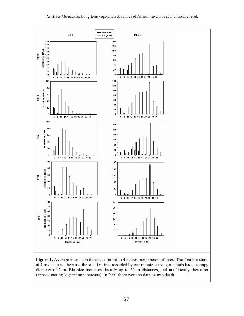
Aristides Moustakas: Long-term vegetation dynamics of African savannas at a landscape level.
Figure 1. Average inter-stem distances (in m) to 4 nearest neighbours of trees. The first bin starts at 4 m distances, because the smallest tree recorded by our remote-sensing methods had a canopy diameter of 2 m. Bin size increases linearly up to 20 m distances, and not linearly thereafter (approximating logarithmic increase). In 2001 there were no data on tree death.
57

Aristides Moustakas: Long-term vegetation dynamics of African savannas at a landscape level.
Distance (m)
6 8 10 12 14 16 18 20 25 30 40
Num
ber o
f tre
es
0
200
400
600
800
1000
1200
dead treesliving trees
Figure 2. Cumulative plot of average inter-stem distances (in m) to 4 nearest neighbours of all trees (all plots and years). The first bin starts at 4 m distances (cf. Fig.1).
58

Aristides Moustakas: Long-term vegetation dynamics of African savannas at a landscape level.
Plot 1
0 10 20 30 40 50 60 70 80 90 100
1940
0,000
0,005
0,010
0,015
0,020
0,025
0 10 20 30 40 50 60 70 80 90 100
1964
0,000
0,002
0,004
0,006
0,008
0,010
0,012
0,014
0 10 20 30 40 50 60 70 80 90 100
1984
0,000
0,002
0,004
0,006
0,008
0 10 20 30 40 50 60 70 80 90 100
1993
0,000
0,002
0,004
0,006
0,008
0,010
Distance (m)0 10 20 30 40 50 60 70 80 90 100
2001
0,000
0,002
0,004
0,006
0,008
0,010
Plot 2
0 10 20 30 40 50 60 70 80 90 1000,000
0,002
0,004
0,006
0,008
0 10 20 30 40 50 60 70 80 90 1000,000
0,001
0,002
0,003
0,004
0,005
0,006
0,007
0 10 20 30 40 50 60 70 80 90 1000,000
0,002
0,004
0,006
0,008
0,010
0,012
0 10 20 30 40 50 60 70 80 90 1000,000
0,002
0,004
0,006
0,008
0 10 20 30 40 50 60 70 80 90 1000,000
0,001
0,002
0,003
0,004
0,005
0,006
0,007
Distance (m)
Figure 3. Temporal change of spatial pattern for all trees larger than 2 m (projected canopy diameter). Solid lines represent the observed g-function with the incorporated heterogeneous Poisson function. The dotted lines represent the upper (clumped) and lower (regular) 99% confidence interval. All results between the two dotted lines cannot be distinguished from random tree distribution. As we used a heterogeneous Poisson method, deviation from CSR is only detectable within R=40 m (see methods).
59

Aristides Moustakas: Long-term vegetation dynamics of African savannas at a landscape level.
Year 1940 1964 1984 1993 2001 Plot 1 Relative tree cover (%) 0.78 0.72 0.75 0.84 0.91 Total trees 370 230 325 361 526 Dead trees 74 25 14 29 New trees 23 120 50 194 Plot 2 Relative tree cover (%) 0.95 1.40 2.65 2.02 1.36 Total trees 621 691 1078 855 817 Dead trees 80 35 253 60 New trees 150 422 30 22
Table 1. Tree characteristics for each different plot and period (data from Moustakas et al. in press). For each plot and for each period (year) we list the relative area covered by tree canopies (Relative tree cover in %), the total number of trees (Total trees), the number of dead trees (Dead trees), and the number of new trees (New trees). Dead trees refer to the interval, namely the 1940 deaths derive from the dead trees between 1940-1964. The other statistics refer to the year the picture was taken. So we always refer back to the last time that the dead trees were seen. In plot 1 during 1940-1964, 89 trees were cut by the farm manager.
60

Aristides Moustakas: Long-term vegetation dynamics of African savannas at a landscape level.
CHAPTER 5: A spatially explicit savanna model along a soil and precipitation gradient. Are savannas cyclothymiacs?
Aristides Moustakas1, Konstantinos Sakkos2, Kerstin Wiegand1, David Ward3, Katrin M.
Meyer1 and Dirk Eisinger4
1. Institute of Ecology, Friedrich Schiller University, Dornburgerstr. 159, 07743 Jena, Germany 2. Departament de Fisica i Enginyeria Nuclear, Universitat Politecnica de Catalunya, Campus Nord B4-B5, E-08034 Barcelona, Spain 3. School of Botany & Zoology, University of KwaZulu-Natal, P. Bag X1, Scottsville 3209, South Africa 4. Department of Ecological Modelling, UFZ-Centre of Environmental Research, P.O. Box 500136, 04301 Leipzig, Germany This chapter will be submitted to Ecological Modelling Abstract
Savannas are ecosystems characterized by the coexistence of woody species (trees and bushes) and grasses. Savanna life cycles are not quantified yet known to be long. Given that savanna characteristics are mainly formed from competition herbivory, woodcutting, and patchy soil and precipitation characteristics, in this paper we propose a spatially explicit model to spatially examine the effects of the abovementioned parameters on savanna vegetation life cycles and vegetation patch dynamics. Furthermore, we test the effects of the abovementioned parameters on tree-bush-grass ratios, as well as the degrees of aggregation of tree-bush-grass biomass. We parameterized our model on an arid savanna with shallow soil depth as well the mesic one with generally deeper and more variant soil depths. Our results showed savanna vegetation varied from open savanna to woodland and back to open savanna again. Vegetation cycles varied over ~300 y cycles on the arid end and ~220 y cycles on the mesic simulated savanna. Our results imply that apart from nutrients cycles and climatic variability there are vegetation cycles too. Part of the vegetation cycle contains a period of higher woody species biomass. Thus, management measures will have to be developed that contain woody species aggregation at its natural level. Overall our findings support that savannas are patch-dynamic systems
Keywords: savanna; spatially explicit; model; patch dynamics; vegetation cycles; 1. Introduction
Savannas are ecosystems characterized by the coexistence of woody species (trees and bushes) and grasses (Scholes and Archer, 1997). The ratio between grass and woody vegetation as well as the total aboveground biomass characterizes the facies of savanna.
61

Aristides Moustakas: Long-term vegetation dynamics of African savannas at a landscape level.
Theoretically, tree-grass coexistence is possible if competition within life forms (tree-grass) is stronger than competition between life forms (Scholes and Archer, 1997). In savannas usually the limiting factors are soil moisture and nutrient availability (Scholes and Archer, 1997). Savannas have annual precipitation that can vary from as little as 100 mm per year to 1300 mm per year (Belsky 1990). Rain has a high degree of patchiness in time and space (Zucchini et al. 1992; Ward et al. 2004). Germination and seedling survival of trees and bushes depends mainly on soil moisture, making recruitment episodic and rare (Sy et al. 2001; Barnes 2001a). Thus, soil moisture is a key factor for savanna vegetation (Laio et al. 2002). Soil moisture itself is mainly a function of rainfall and soil properties such as porosity, water holding capacity and soil depth (Rodriguez-Iturbe et al. 2001; Fernandez-Illescas et al. 2001). These soil properties are patchily distributed within the savanna landscape (Scholes, 1990).
Fire plays an important but unclear role in savanna ecology since there are several contradictive studies on the effect of fire on savanna vegetation (Higgins et al. 2000; Russell-Smith et al. 2003). Even though fire has been proposed as a factor explaining tree-grass coexistence in savannas, the general applicability of this results is questionable. In arid savannas the grass fuel load is often too low to support fires (Bond and Midgley, 1995). Grazing, browsing, and woodcutting play an important role in savannas since selective suppression of some species favours the dominance of other species (Walker et al. 1987; Shipley et al. 1999).
Woody invasion, i.e. the suppression of grassy species by woody plants often unpalatable to livestock, reduces the livestock carrying capacity and biodiversity of savannas and is a widespread economic and ecological problem (Moleele et al. 2002; Meik et al. 2002). Woody invasion is a phenomenon observed in African (O’Connor and Crow, 2000) as well as in American (Archer 1989) and Australian (Burrows et al. 1990) savannas. The causes of woody invasion (in South Africa often referred as “bush encroachment”) are poorly known (Ward, 2005). There are several studies trying to explain the phenomenon (e.g. Polley et al. 2002; Bond et al. 2003; Teague et al. 2004). Global change of CO2 levels favours growth of woody species rather than grassy species leading to bush encroachment while other theories suggest that the phenomenon is caused by overgrazing and/or fire frequency. Management techniques to prevent bush encroachment have been proposed (e.g. Winter, 1990; Teague et al. 2004). The techniques proposed focus mainly on grazing density and frequency. Given that savanna soil and vegetation cycles outlive researchers (Bernhard-Reversat, 1982) it is difficult to predict future scenarios over savanna landscape patterns and vegetation composition. Therefore modelling is a good tool for predicting future scenarios.
Much of the difficulty in savanna modelling and management arises from dealing with very different scales in time, space, and species interactions. Multiple spatial scales are particularly difficult to address using differential equations, because these models focus mainly on population dynamics but not on their spatial distribution. An alternative approach is to focus on the spatial distribution of trees, grass, and bushes, and to develop models which focus on the factors affecting their growth based on their neighbouring situation, rather than trying to add interaction mechanisms to models based on more uniform population dynamics. One way to do this is by the use of grid-based simulation models. In these models, a grid of cells represents the spatial distribution of vegetation,
62

Aristides Moustakas: Long-term vegetation dynamics of African savannas at a landscape level.
e.g. cells may be occupied by grass, bushes, or trees (e.g. Jeltsch et al. 1996). Grid-based discrete time models depict spatial dynamics with rules describing how the occupancy of the grid cells changes from one time step to the next. In classic cellular automata, the state of each cell depends only on the content of it and adjoining cells during the previous time step (Wolfram, 1983; Ermentrout and Edelstein-Keshet, 1993). In contrast, in grid-based models, spatial interaction is possible on all scales.
Due to the advantages of spatially explicit models in such heterogeneous environments as savannas, savanna models are increasingly often spatial (e.g. Jeltsch et al. 1996; Higgins et al. 2000). While there are several good savanna models, there is still space for improvement as a combination of competition-based and demographic modelling approach is needed (Sankaran et al. 2004). Furthermore, most models focus either on one location exclusively, and/or they assume spatial homogeneity in terms of soil properties and moisture characteristics. Good reviews of existing models are given by Belsky (1990) and Sankaran et al. (2004).
The savanna globally reported increase of woody species (Sankaran et al. 2005), is not well understood (Ward 2005). As a result there is a need for a new theory explaining savanna dynamics. Recently, Gillson (2004a; 2004b) and Wiegand et al. (2005; 2006) developed the idea that savannas are patch dynamic systems. According to this theory, savannas are patch-dynamic systems composed of many patches (each patch is comprised of a surface size) in different states of transition between grassy and woody dominance. While evidence is found that savannas are patchy (Gillson 2004a; Wiegand et al. 2005), the spatiotemporal dynamics of the patchiness might be a key to understanding tree-grass coexistence in savannas (Wiegand et al. 2006).
Given that a key to understanding savanna dynamics may lie in recognizing their patchiness (Wiegand et al. 2006), we propose a spatially explicit model that includes spatial variance of precipitation and soil characteristics on large spatial scales and their effect on the aboveground biomass patchy characteristics. The aim of this paper is to introduce the model and to investigate basic properties of the spatiotemporal vegetation dynamics exemplified by two model parameterizations, representing an arid and a mesic savanna. 2. Problem Formulation 2.1. Overview
The purpose of the model is to improve our understanding of the ecology of savannas based on the patch dynamics paradigm. To keep things simple, we focus on two hierarchical levels: vegetation patches and landscape. The specific aim of the model is to better understand the interaction between rainfall, soil, fire, grazing, and plant dynamics as they influence the spatiotemporal development of the patch-dynamic savanna on a landscape scale.
Despite the general interest in nonlinear dynamics in animal populations, plant populations are often believed to show a stable equilibrium. However, the existence of possible vegetation cycles may have been overlooked because empirical studies usually are too short and most modelling studies ignore important spatial aspects of local competition and establishment (Bauer et al. 2002). However, there are several cases of
63

Aristides Moustakas: Long-term vegetation dynamics of African savannas at a landscape level.
cyclical transitions observed in different ecosystems (Loreau, 1997; Bauer et al. 2002; Crespi, 2004), including savannas (Gillson, 2004b; Wiegand et al. 2005). Thus we also tried to detect possible vegetation cycles in savanna ecosystems as a function of precipitation and soil properties.
Based on this purpose, we decided on a grid-based model to follow the dynamics of three life forms (trees and bushes individual based and grass biomass within a cell). The model represents part of a savanna by a rectangular grid of cells. Each cell is characterised by a number of trees and bushes and grass biomass. Each tree and bush has a unique biomass (size) and age. Grass is characterized by grass biomass only. Additionally, each cell has a value of soil porosity and soil depth. The biomass of trees, bushes, and grass in each cell changes on a daily basis through a set of rules. These rules are the key part of the model and are intended to represent the dynamics of savanna vegetation as realistically as possible while staying simple.
For the simulations shown in this paper, we chose a grid (X, Y) of 100 x 100 cells. Each cell corresponds approximately to 3 km on a side, giving a total area of about 90,000 km2. The cell is updated with a daily time step, meaning that the trees, bushes, and grass might grow on a daily basis depending on soil moisture and seasonality. For this paper, we set the number of simulation years (S) to 2000 years. The model follows the state variables biomass (tree and bush individuals, grass biomass) and biomass removed due to burning, grazing, and woodcutting. From this information, we calculate indices of spatial and temporal biomass distribution such as the coefficient of variation of biomass (CV), and spatial & temporal autocorrelation. Thus, this model takes spatial variation into account to a greater extent than most other models.
2.4. Vegetation properties
Several size-classes of bushes and trees can exist within each cell. Thus each cell represents a savanna patch even though several cells together can form a larger savanna patches too.
There is a within-cell limit for the total biomass of each life form (tree, bush, and grass). In addition, tree and bush individuals are attributed by size and age. Grass has only a size as an attribute, which corresponds to grass biomass. This rule is based on the idea that vegetation biomass is constrained by environmental conditions, predominantly rain and active soil depth (Wiegand et al. 2005). To make the model applicable to different environments, we have developed a formula to determine the cell’s upper biomass limit. The maximum biomass of each life form (max_tree_mass, max_bush_mass, max_grass_mass) depends on average annual precipitation (R), soil depth (z), and a water-biomass-conversion-efficiency factor (Ct, Cb, and Cg for trees, bushes, and grass, respectively).
For trees, maximum biomass on a cell is restricted by: RzCtmasstree ××≤_max_
with similar equations for bushes and grass being obtained by substitution. We modelled maximum biomass on a cell using the above formula because on savannas soil
64
Aristides Moustakas: Long-term vegetation dynamics of African savannas at a landscape level.
depth and precipitation are usually the limiting factors (Williams et al. 1996). Maximum biomass of the three life forms is independent from each other in the above formula because in a stable savanna state intraspecific competition is higher than interspecific competition (Higgins et al. 2000). Indirect interspecific competition is included in our model via competition for soil moisture.
Grass biomass is measured in g/m2. As plant growth is size-dependent (Lieberman et al. 1985), we have applied an exponentially declining growth rate as a function of size. It is also well known that height, stem circumference, and canopy area are interrelated (Harper, 1977; c.f. Chapter 3). Even though in our model when referring to “size” we always use biomass indexes (g/m2), in Table 1 we list tree, bush, and grass size in terms of height (m) since it is more comprehensive for the reader.
The model does not include seed dispersal or seed longevity. We assume that given that there is sufficient level of soil moisture at a sufficiently long period of time, there will be germination. As far as the seed dispersal is concerned, this is a quite realistic simplification, since much seed dispersal in savannas occurs from animals that carry seeds for long distances (Barnes, 2001b). From data presented from Witkowski and Garner (2000), seed longevity in most cases is not expected to be the limiting factor for germination.
3. Rule set
The savanna model consists of modules that affect the spatially-explicit population dynamics of the vegetation in each cell (Fig. 1). The dynamics of each vegetation component (trees, bushes, and grass) is followed with two variables (size and, for woody plants, age). Soil moisture is a key variable mediating the effect of many factors and processes on vegetation dynamics. In addition, the model consists of four abiotic (temperature, rain, fire, seasonality), two biotic (grazing, woodcutting & browsing) and three life-history event modules (germination, growth, mortality; Fig. 1). In the following, we describe the rules of/for these modules. The model flow update is graphically represented in Figure 2. A full list with all input parameters is given in Table 1.
65

Aristides Moustakas: Long-term vegetation dynamics of African savannas at a landscape level.
Figure 1. Idealized spatially explicit savanna model along a soil and precipitation gradient. Size and growth are connected because they are interrelated. Arrows show influence of the starting process (box) to the one connected. 3.1. Soil properties
The ecohydrological role of soil texture in water-limited environments is very important (Fernandez-Illescas et al. 2001) and soil properties are very important for savanna plants since in most cases soil quality is poor (McCown and Williams, 1990; Scholes 1990). Soil is modelled as a horizontal layer of depth Z (in cm) (Laio et al. 2001) and porosity n. Soil porosity gives a measure of the difficulty that water has to penetrate the soil and it is dimensionless (Rodriguez-Iturbe et al. 2001). Larger porosity values indicate that more water may enter into the soil. The product of soil depth and porosity nZ defines the active soil depth, which is the depth available for water storage (Laio et al. 2001). Each cell has its own values of porosity and soil depth, which is kept constant during a simulation. According to Blackmore et al. (1990) vegetation patchiness follows soil patchiness which is a persistent result of land use during the past years. In order to test the effect of soil properties on savanna vegetation patchiness, we investigate three soil property scenarios:
(1) Homogeneous soil layer: Soil depth and porosity are identical for all cells.
(2) Patchy soil layer: Each cell has porosity and soil depth values randomly distributed around a mean value of porosity and a mean value of soil depth.
66

Aristides Moustakas: Long-term vegetation dynamics of African savannas at a landscape level.
(3) Soil gradient: We used a gauss function to generate a soil porosity gradient and a gauss function to generate soil depth gradient. The mean value of porosity and soil depth respectively, as well as their variance and the spatial centre of the gauss functions are input parameters.
For the purpose of this paper we used patchy soil layer characteristics. Further details on porosity and soil depth values are given on the model parameterization section and on Table 1.
3.2. Temperature
It is common for savannas to have a strong variation of temperature between winter and summer months (Ogutu and Owen-Smith, 2003), while spatial variability is negligible. From data derived from the South African Weather Bureau for 6 different stations [data from 1940-2003], we tried to find a function that fits to the data. We found that a sinusoidal function fits the data with error that doesn’t exceed +/- 0.5o C. The function updates temperature on a daily basis and all cells have the same temperature during a day. The form of the abovementioned formula is:
]2
minmax)1)[(sin(min TTfTfNoiseTTemp −×++++=
where Temp is the current day’s temperature, Tmin is the minimum annual
temperature occurring on average at the modelled area, π××
−=
23651dayTf , 3651 ≤≤ day
and2
07.0 π−=f . The noise in temperature displacement over the year is:
2)1,0( TdevTdevUNoise −×= , where Tdev is the standard deviation of the temperature
through the year, and U(0,1) is a random number in (0,1).
3.3. Rain characteristics
Precipitation in savannas is highly variable (Williams et al. 1996). We account for this by generating daily rainfall data with different long term mean annual precipitation on the basis of the algorithm by Zucchini et al. (1992). Savannas with lower rainfall, however, tend to have a higher degree of rain patchiness (Ward et al. 2004), a pattern which can not directly be generated with Zucchini’s algorithm, but does influence the vegetation structure of savannas. To allow spatial variability in the rainfall pattern we modified the algorithm by introducing clouds of fixed sizes which resemble the spatial correlation of rainfall in a given region. As the cloud size is smaller than the area modeled, we add additional clouds of the same storm depth but different random location until the cumulated area covered by clouds equals the size of the area modeled. Consequently, not all the simulation cells receive rain, though it does rain in the region, while some cells may receive rain twice the same day. Thus, we adjusted the rainfall probabilities and the rainfall amounts in such a way that in any cell the rainfall
67

Aristides Moustakas: Long-term vegetation dynamics of African savannas at a landscape level.
characteristics equal Zucchini’s model on long term, though the rainfall differs between the cells on a daily basis (see appendix A). The modelling approach used by Zucchini et al. (1992) is the optimal for fitting patching rainfall problems (Makhuvha et al. 1997). The mean annual precipitation (R) is user defined input parameter in our model. The rest of the parameters used for creating rainfall are the ones described by Zucchini et al. (1992).
3.4. Soil moisture properties
Relative soil moisture S takes values in [0,100] and is updated on each cell on a daily basis according to the formula:
)()()1( tSZnWtRtS +
×−
=+ , 0≤S(t+1)≤100
Where, S(t+1) is the cell’s relative soil moisture of the current day, S(t) is the cell’s relative soil moisture of the previous day, R(t) is the rain that fell on that day on the cell, n is soil porosity of the cell, Z is the soil depth of the cell and W(t) the total water losses (leakage, transpiration, evaporation and runoff). The relative soil moisture formula was simplified from Laio et al. (2001). The major difference in our modelling approach is that we include all water losses in one factor W(t) of the form:
W(t) = CwTS(t)
where T is the temperature of that day, and Cw describes the water loss per ºC.
3.5. Fire characteristics
At the spatial and temporal scales considered in out model, we may assume that small fires do not have an important influence on the vegetation. Therefore, once a fire has started, we assume that it is strong enough to burn all grass biomass and all bushes and trees smaller than a threshold size. In addition, soil moisture of that cell is set to 0. There is a minimum fire-resistant size of trees (Frts) and bushes (Frbs).
In our modelling approach, fire ignition (Fi) and spread are influenced by the variables grass biomass, seasonality, soil moisture, possible fire on a neighbouring cell (the chance increases with the number of burning neighbours), and a stochastic element. Seasonality affects fire ignition because fires are more likely to occur when the grass is drier. In order to model seasonality, we assign a gauss function with the peak fire likelihood located at the drier days of the year, i.e. June in our study sites. On a daily basis, a randomly chosen cell is examined whether it exceeds the flammability index using the formula given below. After fire ignition on a cell, it is then examined if fire can spread on the 8 neighbouring cells. For each cell, a flammability index Fi describing the probability of fire ignition is calculated and compared to a fire ignition threshold Fie. We also use a random number r in [0, 1] influencing fire ignition. The flammability index is:
Fi = fire1 × grass biomass + fire2 × seasonality + fire3 × fire on neighbouring cell + fire4 × soil moisture + fire5 × r.
68

Aristides Moustakas: Long-term vegetation dynamics of African savannas at a landscape level.
The weighting factors firex are constant and r is a random number drawn from a uniform distribution in (0,1). Fie needed for fire ignition is an input parameter.
Long-term fire exclusion plots in savanna of various types indicate increased woody vegetation cover in sites where annual precipitation is > 650 mm (Sankaran et al. 2005). In the arid savannas, rainfall is too low to support fires that are intense enough to prevent the regeneration of bush from coppice and seedling growth and long-term fire suppression does not increase woody cover (Sankaran et al. 2005). In our modelling approach we assume that though small fires exist, they are not very influential on savanna vegetation. Therefore in our model once a fire has started, we assume that it is strong enough to burn all grass biomass and all bushes and trees smaller than a certain size. The minimum fire-resistant size of trees (Frts) and bushes (Frbs), are input parameters in our model.
3.6. Seasonality
Vegetation grows exclusively during the life-form specific growth season (beginning and end date for trees: (Gts, Gte, bushes: Gbs, Gbe, and grass (Ggs, Gge); (Paruelo et al. 1999). Seasonality is an important factor for Acacia germination too (Barnes et al. 1997; Barnes 2001a). We therefore included seasonality as an input parameter. Germination takes place during the specified season exclusively. The beginning and end of the germination season is a different pair of parameter for trees (Gts, Gte), bushes (Gbs, Gbe), and grass (Ggs, Gge).
3.7. Tree, bush, and grass growth and mortality
Growth takes place only when the cell’s soil moisture was above a minimum soil moisture threshold (tree: Htg, bush: Hbg, grass: Hgg) during the current day. Woody plants grow until they reach their maximum size (trees: Mts, bushes: Mbs) and thereafter do not grow any further. They die when they reach their maximum age (trees: Mta, bushes: Mba). Several savanna plants have been reported to have linear growth as a function of time (Wiegand T. et al. 2000). Thus we used a function to describe plant growth of the form:
btdaymasstreeatdaymasstree +×=+ )(_)1(_
Growth of bushes and grass is obtained by substitution in the above formula with constant factors ab, bb for bushes and ag, bg for grass.
There are not many data available on green and dry periods of perennial grass. It is known that there is a typical time for grass to die (McCown and Williams 1990; McKeon et al. 1990). However, it is unknown whether grass could have remained green for longer if there had been more rainfall (McCown and Williams 1990; Burrows et al. 1990). In addition, some grass species are annual, therefore they are bound to die at the end of the season. In order to include perennial and annual grass behaviour in our modelling approach, we introduce a season where grass will die. This option was deactivated in the
69

Aristides Moustakas: Long-term vegetation dynamics of African savannas at a landscape level.
simulations presented in this paper. The period through the year that grass dies is characterized by beginning and ending day.
Once germinated, tree and bush seedlings suffer high mortality (Barnes 2001a). Therefore when tree, bush, and grass are below a critical age Smt, Smb, Smg (and thus characterised as seedlings), and the soil moisture during the last Dtsm days for trees, (Dbsm, Dgsm days for bush and grass) is below a minimum threshold Htss, for trees, (Hbss, Hgss, for bush and grass), the seedlings die.
3.8. Competition
Competition stress is an additional mortality cause (Stoll and Weiner 2000; Stoll et al. 2000; Fetene 2003). The maximum biomass of trees (max_tree_mass) that can be sustained in a area of the dimension of our cell and the biomass of trees present on the cell define the competition index as:
masstreemasstreencompetitiotree
_max___ =
When a mature tree (not a seedling) will be randomly killed. Note that Tt is an input parameter that defines the intensity of tree competition and U(0,1) is a random number in (0,1). The above described process applies for bushes and grass accordingly with competition intensities Tb and Tg, respectively.
,_)1,0( TtncompetitiotreeU ≥×
3.9. Germination
Tree and bush germination in savannas is a rare and episodic event and the main limiting factor to this event is soil moisture (Wilson and Witkowski, 1998; Noe, 2002). Grass germination is not a rare event but it has a high dependency on soil moisture (Sy et al. 2001). Germination takes place when a cell’s soil moisture is at least equal to the minimum soil moisture needed for germination during the last days (Wilson and Witkowski 1998). The minimum number of days and the minimum level of soil moisture needed for tree (Dtg, Htg), bush (Dbg, Hbg), and grass (Dgg, Hgg) germination are input parameters. When tree, bush, or grass seedlings reach a certain age, they are not treated as seedlings any more, but as mature trees, bushes, or grass respectively. The mature tree age is Smt (Smb for bush and Smg for grass size respectively).
The model does not include seed dispersal or seed longevity (cf. 2.4.). We assume that given that there is sufficient level of soil moisture at a sufficiently long period of time, there will be germination. In order to avoid unrealistic germination when there are no or few trees or bushes present that their seeds could disperse, we have reduced the germination probability when the total number of trees or bushes is low. When number of trees present is less than 10% of the maximum number of trees (bushes and grass accordingly) that potentially could be present on the cell, germination probability is reduced by 90%. The density-dependent germination function is active only when the abovementioned germination criteria are fulfilled.
70

Aristides Moustakas: Long-term vegetation dynamics of African savannas at a landscape level.
3.10. Grazing, browsing, woodcutting characteristics
We do not include animals as objects in our model but we model the outcome of their interaction with grass, bushes, and trees. The spatial distribution of animals McNaughton (1985) is aggregated. Furthermore, grazing is more intense in places that were recently burned (Fuhlendorf and Engle, 2004). In addition, bushes or trees that are taller than 2 m are browsed by very few animals such as giraffe or elephants, which are mainly found in national parks nowadays. Therefore, bushes and trees over 2 m are not browsed in the model. Woodcutting usually takes place near communities or farms (Tobler et al. 2003). For the abovementioned reasons we model grazing, browsing, and woodcutting as spatially aggregated processes. We use 3 negative binomial distributions, one for each process, to describe the spatial variation grazing, browsing, and woodcutting intensity. Negative binomial distributions allow spatial aggregation. Particularly for grazing, the choice of the cell that will be grazed during the following time step is biased to places that were burned during the last year. The input parameters for each of the 3 distributions are the centre of the activity (Xc, Yc) (Xg, Yg) (Xb, Yb), the mean (rc, rg, rb) and variance (pc, pg, pb), as well as the number of activities per day (Nc, Ng, Nb). For example, when the number of woodcutting activities per day Nc is set to 2, then 2 cells will be chosen according to the negative binomial distribution centred around (Xc, Yc) with mean rc and variance pc and trees will be killed on each cell accordingly. Arid savannas support less humans and animals than mesic ones. We therefore assumed that numbers of daily grazing, browsing, and woodcutting activities are lower in arid savanna. The grazing centre is adjusted to fire by keeping in memory the burned cells during the past two years. The abovementioned grazing distribution is biased by favouring 20% higher chances of grazing into cells that were burned within the last two years.
4. Initialization
Soil depth and porosity values are given on each cell according to the distribution chosen (constant, gradient, and gauss). Soil depth and porosity values, once distributed on each cell, remain constant during a simulation period. Furthermore, on each cell a value of grass biomass as well as a number of trees, bushes are given. The size and age of each tree and grass are randomly chosen. Number of trees and bushes on a cell can never exceed the maximum number of trees and bushes on a cell, respectively. In addition, tree and bush age and size do not exceed maximum tree or bush size and age. Also grass biomass distributed on each cell will not be larger than the maximum grass biomass on a cell. According to the parameterisation of the model, some years of simulation period are necessary for the model to generate a realistic savanna pattern. We keep statistics of tree, grass, and bush biomass after the initial simulation period (Sss).
71

Aristides Moustakas: Long-term vegetation dynamics of African savannas at a landscape level.
Figure 2. Flow chart of the spatially explicit savanna model. Initialization sets the default values of soil depth, porosity and the initial values of tree, bush, and grass location, size, and age. Sequentially, for each time step (one day), the amount of rainfall on each cell and the temperature are calculated in order to set the cell’s soil moisture. Under sufficient soil moisture and during the right season, growth and germination take place, meanwhile seedling mortality occurs when soil moisture is lower than the minimum moisture needed for survival (regardless of the season). After that, some mature trees bushes and grass could die due to competition and depending upon the vegetation density. Sequentially, grazing, browsing, and woodcutting activities take place and reduce tree, bush, and grass biomass. Lastly, fire could ignite depending mainly upon grass biomass and seasonality. Fire burns all grass and all small trees and bushes on the cell.
5. Output
In order to assess data on spatial statistics, we record on each cell the tree, bush, and grass biomass. On the same time interval we also record on each cell the biomass removed due to herbivory (grazing, browsing) and woodcutting, as well as the burned tree, bush, and grass biomass. We calculate the mean and coefficient of variation of all the abovementioned characteristics. The coefficient of variation (CV) is frequently used as an index of spatial size variability of individuals (Li et al. 1996). Similarly, applying the CV on the abovementioned spatial attributes, one can use the CV as a measure of patchiness.
Spatial autocorrelation is a very appropriate index of measuring patches and gradients (Legendre 1993). Therefore, we calculate spatial autocorrelation using Moran’s index (for details see Overmars et al. 2003) in 10 user-defined cells. To detect possible cycles, we also calculated autocorrelation in time in 10 user-defined cells every 20 years.
72

Aristides Moustakas: Long-term vegetation dynamics of African savannas at a landscape level.
6. Model parameterization
In this paper, we parameterize the model for two exemplary savanna systems: arid and mesic. Apart from the obvious difference of the mean annual precipitation levels between the two sites, there are several other differences between arid and mesic savannas. Soil quality expressed in our model as porosity and soil depth are usually different between arid and mesic environments. Arid environments usually have lower soil depth and porosity values. Fire is considerably lower in arid environments because there is not sufficient grass fuel to support large fires. Therefore arid landscapes are less fire-driven than mesic ones. In arid environments, percentage of plant cover is low. As a result, there is less available food and thus less animals and human population per hectare. Therefore, grazing, browsing, and woodcutting activities are less frequent (but not necessarily less intensive). Published data were used about the tree, bush and grass growing season (Barnes et al. 1997; Golluscio et al. 1998; Veenendaal et al. 1996).
The arid study area is located west of Windhoek on the western edge of the Khomas Hochland, Namibia on three adjacent ranches: Quabis, Tweespruit, and Changans. These ranches are situated between two parallel mountain ranges. There is a shallow layer of sandy soil overlying Swakop schist from the Damara sequence. Thus, roots of both woody and grassy plants are confined to a thin soil layer (< 5─15 cm deep). Rain falls in summer (January – April) and is very patchy. Mean annual precipitation is 122 mm (±50) Tree and bush germination period on the area is mainly January - March, and grass germination period is September – March. Growth season for tree and bush species is mainly November – March meanwhile for grass is September - March. More details on the study area are given by Ward et al. (2004).
The mesic study area is located at the Serengeti plains, Tanzania. We mainly focused on the area around Banagi. Rain falls mainly from November – May. Rain is patchy and highly varying through years; mean annual precipitation is 780 mm (±283). The area around Banagi is generally bushland and woodland. Soil is mainly brown calcareous and soil depth is patchy. Minimum soil depth is 20 cm but in some places roots are still common in depths of up to 200 cm. Tree, bush, and grass germination period on the area is mainly September - March. Growth season for tree and bush species is mainly November – March, meanwhile grass growth is September - March. A detailed description of the area including tables of soil and vegetation characteristics is given by Anderson and Talbot (1965).
7. Results
Overall tree, bush, grass, and total biomass showed a cyclic behaviour through time (Fig. 3; Fig. 4). Grass life cycle is about three years, bush life cycle is on average 50 y, and tree life cycle is on average 200 y (results not shown here). The total aboveground biomass is the combined effect of the grass, bush, and tree cycles. As a result, starting from an open savanna with scattered trees and bushes, there is a period were savanna vegetation generally decreases due to climatic variations, then there is a period when savanna becomes a woodland with further increase of woody species, and then a period where savanna becomes more open again. The periodic transition from open to more
73

Aristides Moustakas: Long-term vegetation dynamics of African savannas at a landscape level.
encroached savanna (more woody species) was a general result of both the arid and mesic savanna. However, in our simulations, the period of a cycle was ~300 y in the arid savanna and ~230 y periods in the mesic savanna (Fig. 4).
Figure 3. Snapshots of savanna vegetation pattern over 300 years simulation-cycles. Lighter colour depicts lower biomass values. There is a periodical transition from an open savanna (upper left) to a scarcely-vegetated savanna (upper right) sequentially to a highly vegetated savanna with closely spaced species (down middle), to an open savanna again (down right). The results shown here are taken from the simulation of the arid savanna shown in Fig. 4. Similar cycle and pattern is observed in the simulated mesic savanna too. Snapshots shown here were taken at (years) t=720, 840, 900, 960, and 1020 (cf. Fig. 4).
Overall, tree biomass was higher than bush biomass in the arid savanna but bush biomass outweighted tree and grass biomass in the mesic simulated savanna (Table 2). Tree biomass did not differ much between arid and mesic simulations. However, grass and bush biomass were affected by the difference in precipitation. Bush biomass was doubled in the mesic savanna and grass biomass was increased almost 7 times. Both variance and CV of tree biomass was higher at the mesic savanna. Therefore, tree patches are more unpredictable in the mesic savanna. Bush biomass variance increased
74

Aristides Moustakas: Long-term vegetation dynamics of African savannas at a landscape level.
impressively at the mesic savanna. However bush CV increased not at the same level. Therefore, even though in the mesic savanna there were bushes in more places than in the arid savanna, patches are more unpredictable and patch size more uneven. Even though grass biomass variance decreased in the mesic savanna, grass CV increased. Therefore grass patches in the mesic savanna had similar sizes but the degree of grass patchiness increased (Table 2).
Temporal autocorrelation of tree values revealed changing structure of tree populations over time (Fig. 5a). Tree biomass in the arid savanna was less correlated than in the mesic savanna. Therefore temporal behavior of tree patches was more unpredictable in the arid environment. However, the fluctuations in the autocorrelation with distance of tree biomass were greater in the arid savanna than in the mesic savanna (Fig. 5d). Spatial autocorrelation analysis of trees showed that neighboring savanna tree patches are similar. However, similarity of patches that are far from each other is greater than at intermediate distances.
Bush temporal autocorrelation analysis showed similar unpredictability in arid as well as in mesic savanna (Fig. 5b). However, in arid savannas there seems to be a period where bush biomass becomes highly correlated (about 800 years; Fig. 5b). Spatially (Fig. 5f), like tree patches, neighboring bush patches seem to be similar, intermediate bush patches are less similar, and distant bush patches become similar again.
Grass temporal behavior was almost stable in both the arid and mesic simulated savanna (Fig. 5c). However, in space, grass showed similar results as trees and bushes, but to a lesser extent: grass patches are fairly similar when close to each other, less similar at intermediate distances and their similarity increases as distance increases (Fig. 5g). The grass biomass in the mesic savanna had always higher autocorrelation than in the arid savanna.
7. Discussion
Our model was able to reproduce savanna vegetation characteristics for periods of time over 2000 years with daily updated time steps. Jeltsch et al. (1996), using spatially explicit simulations, found that higher rainfall increased woody recruitment and the simulated savanna turned into woodland. This result lead Jeltsch et al. (1996) to the conclusion that “factors or processes other than competition for moisture, herbivory and fire are needed in addition to induce a long-term persistence of scattered trees”. Using our modeling approach, increased precipitation did not turn the simulated savanna into woodland. Fire, grazing, browsing, and woodcutting are often suggested to be the main driving forces (e.g. Van de Koppel and Prins 1998). Even though they affected patchy vegetation characteristics, according to our findings they were not as important (results not shown here). On the other hand, our results comply with O’Connor (1993), who found that “an extrinsic force presumably rainfall had the greatest effect on population growth”.
75

Aristides Moustakas: Long-term vegetation dynamics of African savannas at a landscape level.
7.1. Results on a gradient basis
Our mesic savanna had on average higher precipitation, porosity and soil depth values than the arid one due to our parameterization. The increase of woody biomass increased in our simulations when the soil’s porosity values used in simulation were increased (mesic savanna), in combination with higher precipitation. Williams et al. (1996), measuring the composition and structure of tropical savannas as a function of precipitation and soil texture, found that tree height declined with decreasing rainfall, which is in agreement with our findings. In the same study, it was also found that cover, and basal area of woody species declined with decreasing rainfall and increasing soil clay content. Clay has a high porosity and moisture value in comparison with other types of soil (Fernandez-Illescas et al. 2001). In our arid savanna, soil is shallow and with low porosity values, while usually the opposite is valid for our mesic simulated savanna even though soil properties are patchily distributed. According to our findings the ratio of bush/tree biomass is much higher in the arid savanna (Table 2). Thus, even though our results do not prove any necessary implication between precipitation, porosity, and bush biomass, common findings with Williams et al. (1996) are found.
7.2. About savanna vegetation cycles
Using a grid based model of savanna vegetation dynamics in the Kalahari, Jeltsch et al. (1997) concluded that, although the stocking rates recommended by pasture scientists are unlikely to lead to shrub encroachment within 20 years, they have a high probability of bringing about shrub encroachment within a century. According to our findings, there is no way of avoiding a shrub encroachment within two centuries. The fact that we found a periodicity in savanna vegetation dynamics supports the hypothesis that savannas are patch-dynamic systems (Gillson, 2004a; Wiegand et al. 2006) with bush encroachment as an integral part of their dynamics (Wiegand et al. 2006). According to our results, there is a spatial and temporal variation of the savanna facies. Temporally, a patch will pass through an encroached face and sequentially to a more open savanna one, till it is encroached again. Spatially, when a savanna is viewed at a specific time step, there are some encroached patches, while some other patches are comprised of an open savanna. Furthermore, our finding that tree and bush patches are similar in larger than intermediate distances, implies that, some parts of a savanna always contain some patches with increased woody species biomass. In that case, we will have to accept that there will always be some bush encroachment. Management measures suggesting grazing frequency and intensity (e.g. McKeon et al 1990; Moleele et al. 2002) should not aim to completely eradicate bush encroachment unless we want to destroy savanna systems, turning them into pure grasslands for pastoral use.
It is well reported that savanna nutrients are characterized by cycles (Bernhard-Reverserat 1982; Boutton et al. 1999). Our results imply that there are vegetation cycles too. If the existence of vegetation cycles is valid, then the whole interpretation of vegetation changes and management should be decoded taking into account these cycles. Thus, management measures will have to be developed that contain bush encroachment
76

Aristides Moustakas: Long-term vegetation dynamics of African savannas at a landscape level.
at its natural level, which ensures that there are some patches of bush encroachment (good for the future state of the savanna), but not too many (good for livestock). Furthermore, one may want to thin patches of bush encroachment to a point that conserves the positive effect of nutrient enrichment by encroaching trees but reduces suppression of grasses due to competition for water.
Time (years)
200 400 600 800 1000 1200 1400 1600 1800 2000
Tota
l bio
mas
s (g
/m2 )
1500
2000
2500
3000
3500
mesicarid
Figure 4. Total savanna biomass (tree, bush, and grass) over 2000 simulation years. Results are updated every 10 years. The lines or dots connecting biomass values every 10 y, do not show intermediate biomass values; they are connected for examining trends. The biomass snapshots shown in figure 3 are referring to the arid savanna and taken in years 720, 840, 900, 960, 1020. 7.3. Future development
Climate change is an issue of current concern (Hulme et al. 2001) and can potentially affect savanna vegetation (Skarpe 1996). This model is a useful tool to explore potential savanna vegetation scenarios under different temperature and precipitation parameters.
Many commercial farms in savannas are mainly cattle farms. Cattle are non endemic savanna animals and fairly recently introduced (about 300 y ago). Thus, most animals are
77

Aristides Moustakas: Long-term vegetation dynamics of African savannas at a landscape level.
grazers, while only game farms contain animals that are browsers. It therefore would be interesting to investigate the effect of browsing vs. grazing ratio on savannas. There are several suggestions that propose some better grazing strategies to avoid land degradation (e.g. Moleele et al. 2002; Archer 2004). However, it would be very interesting to examine the effect of keeping the total animal biomass on a farm constant but replace some grazers with browsers on savanna vegetation and woody species in particular.
On the whole, fire also added to vegetation patchiness. Especially since places that were recently burned were more likely to be grazed, fire as a process had a multiple effect on vegetation patchiness (results not shown here). However, fire was not able to stop savannas’ vegetation cyclical transition once again. Thus it would be interesting to run simulation scenarios about the role of fire on savanna patch dynamics.
The effect of grazing on grass is clear and generally increases savanna clumped characteristics. However it remains unclear whether grazing favours the aggregation of woody species on larger spatial scales. Furthermore grazing as a process has an unknown effect on savannas’ cyclical transition from open savanna to woodlands. We therefore plan to run simulation scenarios investigating the role of herbivory on savanna patch dynamics.
References Anderson, G.D., Talbot, L.M., 1965. Soil factors affecting the distribution of the
grassland types and their utilization by wild animals on the Serengeti plains, Tanganyika. The Journal of Ecology 53, 33-56.
Archer, E.R.M., 2004. Beyond the "climate versus grazing" impasse: using remote sensing to investigate the effects of grazing system choice on vegetation cover. Journal of Arid Environments 57, 381-408.
Barnes R.D., Fagg, C.W., Milton, S.J., 1997. Acacia erioloba. Monograph and annotated bibliography. Oxford Forestry Institute, Department of Plant Sciences, University of Oxford.
Barnes, M.E., 2001a. Effects of large herbivores and fire on the regeneration of Acacia erioloba in Chobe National Park, Botswana. African Journal of Ecology 39, 340-350.
Barnes, M.E., 2001b. Seed predation, germination and seedling establishment of Acacia erioloba in northern Botswana. Journal of Arid Environments 49: 541-554.
Bauer, S., Berger, U., Hildenbrandt, H., Grimm, V., 2002. Cyclic dynamics in simulated plant populations. Proceedings of the Royal Society of London B 269, 2443-2450.
Belsky, A.J., 1990. Tree/grass ratios in East African savannas: a comparison of existing models. Journal of Biogeography 17, 483-489.
Bernhard-Reverserat, F., 1982. Biogeochemical cycle of nitrogen in a semi-arid savanna. Oikos 38,: 321-332.
Blackmore, A.C., Mentis, M.T., Scholes, R.J., 1990. The orign and nature of nutrient-enriched patches within a nutrient-poor savanna. Journal of Biogeography 17, 463-479.
78
Aristides Moustakas: Long-term vegetation dynamics of African savannas at a landscape level.
Bond, W.J., Midgley, G.F., Woodward, F.I., 2003. The importance of low atmospheric CO2 and fire in promoting the spread of grasslands and savannas. Global Change Biology 9, 973-982.
Bond, W.J., Midgley, J.J., 1995. Kill thy neighbor - an individualistic argument for the evolution of flammability. Oikos 73, 79-85.
Boutton, T.W., Archer, S.R., Midwood, A.J., 1999. Stable isotopes in ecosystem science: Structure, function, and dynamics of a subtropical savanna. Rapid communications in mass spectometry 13, 1263-1277.
Burrows, W.H., Carter, J.O., Scanlan, J.C., Anderson, E.R., 1990. Management of savannas for livestock production in north-east Australia: contrasts across the tree-grass continuum. Journal of Biogeography 17, 503-512.
Crespi, B.J., 2004. Vicious circles: positive feedback in major evolutionary and ecological transitions. Trends in Ecology and Evolution 19, 627-633.
Ermentrout, G.B., Edelstein-Keshet, L., 1993. Cellular automata approaches to biological modeling. Journal of Theoretical Biology 160, 97-133.
Fernandez-Illescas, C.P., Porporato, A., Laio, F., Rodriguez-Iturbe, I., 2001. The ecohydrological role of soil texture in a water-limited ecosystem. Water Resources Research 37, 2863-2872.
Fetene, M., 2003. Intra- and interspecific competition between seedlings of Acacia etbaica and a perennial grass (Hyparrenia hirta). Journal of Arid Environments 55, 441-451.
Fuhlendorf, S.D., Engle, D.M., 2004. Application of the fire-grazing interaction to restore a shifting mosaic on tallgrass prairie. Journal of Applied Ecology, 41, 604.
Gillson, L., 2004a. Evidence of hierarchical patch dynamics in an East African savanna? Landscape Ecology, 883-894.
Gillson, L., 2004b. Testing non-equilibrium theories in savannas: 1400 years of vegetation change in Tsavo National Park, Kenya. Ecological Complexity 1, 281-298.
Golluscio, R.A., Sala, O.E., Lauenroth, W.K., 1998. Differential use of large summer rainfall events by shrubs and grasses: a manipulative experiment in the Patagonian steppe. Oecologia 115, 17-25.
Harper J.L., 1977. Population biology of plants. Academic Press, New York, USA.
Higgins, S.I., Bond, W.J., Trollope, S.W., 2000. Fire, resprouting and variability: A recipe for grass-tree coexistence in savanna. Journal of Ecology 88, 213-229.
Hulme, M., Doherty, R., Ngara, T., New, M., Lister, D., 2001. African climate change: 1900-2100. Climate Research 17, 145-168.
Jeltsch, F., Milton, S.J., Dean, W.R.J., Van Rooyen, N., 1997. Analysing shrub encroachment in the southern Kalahari: a grid-based modelling approach. Journal of Applied Ecology 34, 1497-1508.
Jeltsch, F., Milton, S.J., Dean, W.R.J.; Van Rooyen, N., 1996. Tree spacing and coexistence in semiarid savannas. Journal of Ecology 84, 583-595.
79

Aristides Moustakas: Long-term vegetation dynamics of African savannas at a landscape level.
Laio, F., Porporato, A., Ridolfi, L., Rodriguez-Iturbe, I., 2001. Plants in water-controlled ecosystems: active role in hydrologic processes and response to water stress - II. Probabilistic soil moisture dynamics. Advances in Water Resources 24, 707-723.
Laio, F., Porporato, A., Ridolfi, L., Rodriguez-Iturbe, I., 2002. On the seasonal dynamics of mean soil moisture. Journal of Geophysical Research 170, 1-9.
Legendre, P., 1993. Spatial autocorrelation: Trouble or new paradigm? Ecology 74, 1659-1673.
Li, B., Watkinson, A.R.; Hara, T., 1996. Dynamics of competition in populations of carrot (Daucus carota). Annals of Botany 78, 203-214.
Lieberman D., Lieberman M., Hartshorn G., Peralta R., 1985. Growth rates and age-size relationships of tropical wet forest trees in Costa Rica. Journal of Tropical Ecology 1, 97-109.
Loreau, M., 1997. Ecosystem development explained by competition within and between material cycles. Proceedings of the Royal Society of London B 265, 33-38.
Makhuvha, T., Pegram, G., Sparks, R., Zucchini, W., 1997. Patching rainfall data using regression methods. 2. Comparisons of accuracy, bias and efficiency. Journal of Hydrology 198, 308-318.
McCown, R.L., Williams, J., 1990. The water environment and implications for productivity. Journal of Biogeography 17, 513-520.
McKeon, G.M., Day,K.A., Howden,S.M., Mott,J.J., Orr,D.M., Scattini,W.J., Weston,E.J.., 1990. Northern Australian savannas - Management for pastoral production. Journal of Biogeography 17, 355-372.
McNaughton, S.J., 1985. Ecology of a grazing system: The Serengeti. Ecological Monographs 55, 259-294.
Meik, J.M., Jeo, R.M., Mendelson III, J.R., Jenks, K.E., 2002. Effects of bush encroachment on an assemblage of diurnal lizard species in central Namibia. Biological Conservation 106, 29-36.
Moleele, N.M., Ringrose, S., Metheson, W., Vanderpost, C., 2002. More woody plants? the status of bush encroachment in Botswana's grazing areas. Journal of Environmental Management 64, 3-11.
Noe, G.B., 2002. Temporal variability matters: effects of constant vs. varying moisture and salinity on germination. Ecological Monographs 72, 427–443.
O'Connor, T.G., 1993. The influence of rainfall and grazing on the demography of some African savanna grasses: a matrix modelling approach. Journal of Applied Ecology 30, 119-132.
O'Connor, T.G., Crow, V.R.T., 2000. Rate and pattern of bush encroachment in Eastern Cape savanna and grassland. African Journal of Range & Forage Science 16, 26-31.
Ogutu, J.O., Owen-Smith, N., 2003. ENSO, rainfall and temperature influences on extreme population declines among African savanna ungulates. Ecology Letters 6, 412-419.
80

Aristides Moustakas: Long-term vegetation dynamics of African savannas at a landscape level.
Overmars, K.P., de Koning, G.H.J., Veldkamp, A., 2003. Spatial autocorrelation in multi-scale land use models. Ecological Modelling 164, 257-270.
Paruelo, J.M., Lauenroth, W.K., Burke, I.C., Sala, O.E., 1999. Grassland precipitation-use efficiency varies across a resource gradient. Ecosystems 2, 64-68.
Polley, H.W., Johnson, H.B., Tischer, C.R., 2002. Woody invasion of grasslands: evidence that CO2 enrichment indirectly promotes establishment of Prosopsis glandulosa. Plant Ecology 164, 85-94.
Riginos, C., Hoffman, M.T., 2003. Changes in population biology of two succulent shrubs along a grazing gradient. Journal of Applied Ecology 40, 615-625.
Rodriguez-Iturbe, I., Porporato, A., Laio, F., Ridolfi, L., 2001. Intensive or extensive use of soil moisture: plant strategies to cope with stochastic water availability. Geophysical Research Letters 28, 4495-4497.
Rodriguez-Iturbe, I., Porporato, A., Laio, F., Ridolfi, L., 2001. Plants in water-controlled ecosystems: active role in hydrologic processes and response to water stress - I. Scope and general outline. Advances in Water Resources 24, 695-705.
Russell-Smith, J., Whitehead, P.J., Cook, G.D., Hoare, J.L., 2003. Response of Eucalyptus-dominated savanna to frequent fires: lessons from Munmarlary, 1973-1996. Ecological Monographs 73, 349-375.
Sankaran, M., et al., 2005. Determinants of woody cover in African savannas. Nature, 438, 846-849.
Sankaran, M., Ratnam, J., Hanan, N.P., 2004. Tree-grass coexistence in savannas revisited - insights from an examination of assumptions and mechanisms invoked in existing models. Ecology Letters 7, 480.
Scholes, R.J., 1990. The influence of soil fertility on the ecology of southern African dry savannas. Journal of Biogeography 17, 415-419.
Scholes, R.J., Archer, S.R., 1997. Tree-grass interactions in savannas. Annual Review of Ecology and Systematics 28, 517-544.
Shipley, L.A., Illius, A.W., Danell, K., Hobbs, T., Spalinger, D.E., 1999. Predicting bite size selection of mammalian herbivores: a test of a general model of diet optimization. Oikos 84, 55-68.
Skarpe, C., 1996. Plant functional types and climate in a southern African savanna. Journal of Vegetation Science 7, 397-404.
Stoll, P., Weiner, J., 2000. A neighbourhood view of interactions among plants. In: U. Dieckmann, R. Law and J.A.J. Metz (Editors), The geometry of ecological interactions: simplifying spatial complexity. Cambridge studies in adaptive dynamics. Cambridge University Press, Cambridge, pp. 11-27.
Stoll, P., Weiner, J., Müller, E., 2000. Size-symmetric competition and density-biomass relationships in a spatially-explicit, individual-based plant competition model, Plant Population Viability Analysis, Weihenstephan.
81

Aristides Moustakas: Long-term vegetation dynamics of African savannas at a landscape level.
Sy, A., Grouzis, M., Danthu, P., 2001. Seed germination of seven Sahelian legume species. Journal of Arid Environments 49, 875-882.
Teague, W.R., Dowhower, S.L., Waggoner, J.A., 2004. Drought and grazing patch dynamics under different grazing management. Journal of Arid Environments 57, 97-117.
Tobler, M.W., Cochard, R., Edwards, P.J., 2003. The impact of cattle ranching on large-scale vegetation patterns in a coastal savanna in Tanzania. Journal of Applied Ecology 40, 430-444.
Trollope, W.S.W., 1982. Ecological effects of fire in South African savannas. In: B.J. Huntley and B.H. Walker (Editors), Ecology of tropical savannas. Ecological studies. Springer-Verlag, Berlin HeidelbergNew York, pp. 292-306.
Van de Koppel, J., Prins, H.H.T., 1998. The importance of herbivore interactions for the dynamics of African savanna woodlands: an hypothesis. Journal of Tropical Ecology 14, 565-576.
Veenendaal, E.M., Ernst, W.H.O., Modise, G.S., 1996. Effects of seasonal rainfall pattern on seedling emergence and establishment of grasses in a savanna in south-eastern Botswana. Journal of Arid Environments 32, 305-317.
Walker, B.H., Emslie, R.H., Owen-Smith, R.N., Scholes, R.J., 1987. To cull or not to cull: Lessons from a Southern African drought. Journal of Applied Ecology 25, 381-401.
Ward, D., 2005. Do we understand the causes of bush encroachment in African savannas? African Journal of Range & Forage Science, 22, 101-105.
Ward, D., Saltz, D., Ngairorue, B.T., 2004. Spatio-temporal rainfall variation and stock management in arid Namibia. Journal of Range Management 57, 130-140.
Wiegand, K., Saltz, D., Ward, D., 2006. A patch dynamics approach to savanna dynamics and woody plant encroachment - Insights from an arid savanna. Perspectives in Plant Ecology, Evolution and Systematics 7, 229-242.
Wiegand, K., Ward, D., Saltz, D., 2005. Multi-scale patterns in an arid savanna with a single soil layer. Journal of Vegetation Science 16, 311-320.
Wiegand, T., Milton, SJ., Esler, KJ., Midgley, GF., 2000. Live fast, die young: estimating size-age relations and mortality pattern of shrub species in the semi-arid Karoo, South Africa. Plant Ecology 150, 115-131.
Williams, R.J., Duff, G.A., Bowman, D.M.J.S., Cook, G.D., 1996. Variation in the composition and structure of tropical savannas as a function of rainfall and soil texture along a large-scale climatic gradient in the Northern Territory, Australia. Journal of Biogeography 23, 747-756.
Wilson, T.B. and Witkowski, E.T.F., 1998. Water requirements for germination and early seedling establishment in four African savanna woody plant species. Journal of Arid Environments 38, 541-550.
Winter, W.H., 1990. Australia's northern savannas: A time for change in management philosophy. Journal of Biogeography 17, 525-529.
Witkowski, E.T.F., Garner, R.D., 2000. Spatial distribution of soil seed banks of three African savanna woody species at two contrasting sites. Plant Ecology 149, 91-106.
82

Aristides Moustakas: Long-term vegetation dynamics of African savannas at a landscape level.
Wolfram, S., 1983. Cellular automata. Los Alamos Science 9, 2-21.
Zucchini, W., Adamson, P., McNeill, L., 1992. A model of Southern African rainfall. South African Journal of Science 88, 103-109.
Temporal Analysis
Time (years)
200 400 600 800 1000 1200 1400 1600 1800 2000
Tree
Aut
ocor
rela
tion
0,070
0,075
0,080
0,085
0,090
0,095
0,100
Time (years)
200 400 600 800 1000 1200 1400 1600 1800 2000
Bus
h A
utoc
orre
latio
n
0,070
0,075
0,080
0,085
0,090
0,095
0,100
Time (years)
200 400 600 800 1000 1200 1400 1600 1800 2000
Gra
ss A
utoc
orre
latio
n
0,0990
0,0995
0,1000
0,1005
0,1010
Spatial Analysis
Distance (cells)
10 20 30 40 50 60 70 80 90 100Tr
ee A
utoc
orre
latio
n
0,070
0,075
0,080
0,085
0,090
0,095
0,100
Distance (cells)
10 20 30 40 50 60 70 80 90 100
Bus
h A
utoc
orre
latio
n
0,070
0,075
0,080
0,085
0,090
0,095
0,100
Distance (cells)
10 20 30 40 50 60 70 80 90 100
Gra
ss A
utoc
orre
latio
n
0,070
0,075
0,080
0,085
0,090
0,095
0,100
0,105
0,110
0,115
0,120
a d
f
b
c
e
Figure 5. Temporal (left graphs) and spatial (right graphs) autocorrelation analysis of tree, bush, angrass biomass respectively. Results of the mesic simulated savanna are dotted. The lines or dots connecting points do not show intermediate autocorrelation; points are connected for examining trends. Each point in the graph shows the autocorrelation values averaged over 10 selected cells. Autocorrelation values were calculated using Moran’s index.
83

Aristides Moustakas: Long-term vegetation dynamics of African savannas at a landscape level.
General characteristics Units Arid Mesic S Number of simulation years years 2000 X Number of cells on X axis dimensionless 100 Y Number of cells on Y axis dimensionless 100 Ct Tree water-biomass-conversion-efficiency factor 105g/m2 16 Cb Bush water-biomass-conversion-efficiency factor 105g/m2 13 Cg Grass water-biomass-conversion-efficiency factor 105g/m2 7 Equilibration period (savanna stable state) years 100 Tree and Bush Characteristics Mta Max. tree age years 250 Mba Max. bush age years 80 Mts Max. tree size m 14 Mbs Max. bush size m 6 Smt Mature tree size m 2 Smb Mature bush size m 0.8 Smg Mature grass size cm 25 optional-no grass period Gn Beginning of period that grass dies months not used Gy End of period that grass dies months not used Ga Activate no grass period 0 or 1 not used Temperature Tmax Max. temperature C0 36 34 Tmin Min. temperature C0 1 5 Tdev St. deviation of temperature C0 20 25 Soil Moisture Mm Max. moisture in a cell % 100 Cm what kind of Constant? of water losses function cm/Co 0.9
N Porosity dimensionless 0.07 (±0.03)
0.10 (±0.05)
Z Soil depth cm 10 (±5) 100 (±80) Growth Gts Beginning of tree growing season month November Gte End of tree growing season month March Gbs Beginning of bush growing season month November Gbe End of bush growing season month March Ggs Beginning of grass growing season month September Gge End of grass growing season month March Htgr Min.. moisture needed for tree growth % 13 Hbgr Min. moisture needed for bush growth % 11 Hggr Min. moisture needed for grass growth % 9 Germination Gts Beginning of tree germination period month January September Gte End of tree germination period month March Gbs Beginning of bush germination period month January September Gbe End of bush germination period month March Ggs Beginning of grass germination period month September Gbe End of grass germination period month March Htg Min. moisture needed for tree germination % 21 Hgg Min. moisture needed for grass germination % 15
84

Aristides Moustakas: Long-term vegetation dynamics of African savannas at a landscape level.
Hbg Min. moisture needed for bush germination % 18 Dtg Days with min moisture needed for tree germination days 5 Dbg Days with min moisture needed for bush germination days 4 Dgg Days with min moisture needed for grass germination days 3 Competition Tt Intensity of tree competition % 0.7 0.8 Bt Intensity of bush competition % 0.6 0.7 Gt Intensity of grass competition % 0.45 0.5 Seedling Mortality Smt Max. tree seedling age years 5 Smb Max. bush seedling age years 4 Smg Max. grass seedling age months 3 Htss Min. moisture for tree seedling survival % 10 Hgss Min. moisture for grass seedling survival % 7 Hbss Min. moisture for bush seedling survival % 9 Dtsm days with min moisture needed for tree seedling mortality days 5 Dgsm days with min moisture needed for grass seedling mortality days 3 Dbsm days with min moisture needed for bush seedling mortality days 4 Fire Fm Mean peak period of fire gauss function month June Fsd St. deviation of fire gauss function month April-August Fsh Sharpness of fire gauss function dimensionless 6 fire 1 Constants of fire formula m2/g 1 fire 2 Constants of fire formula 1/month 0.7 fire 3 Constants of fire formula dimensionless 0.5 fire 4 Constants of fire formula dimensionless 0.5 fire5 Constants of fire formula dimensionless 0.5
Fi Threshold probability of fire ignition % (probability) 0.6
Frts Min. size of fire-resistant trees m 6 Frbs Min. size of fire-resistant bushes m 4 Grazing Browzing Woodcutting Nc Number of daily tree cutting activities dimensionless 1 2 Ng Number of daily grazing activities dimensionless 4 6 Nb Number of daily browsing activities dimensionless 2 3 rt, pt r and p values of neg. binomial tree cutting function dimensionless 1 and 0.2 rg, pg r and p values of neg. binomial grazing function dimensionless 1 and 0.2 rb, pb r and p values of neg. binomial browsing function dimensionless 1 and 0.2 Xc,Yc Centre of neg. binomial tree cutting function dimensionless (10, 30) Xg,Yg Centre of neg. binomial grazing function dimensionless (30, 10) Xb,Yb Centre of neg. binomial browsing function dimensionless (40, 40) Rain
R Mean annual precipitation mm 165 780 Table 1. Summary of model input parameters and simulation values.
85

Aristides Moustakas: Long-term vegetation dynamics of African savannas at a landscape level.
Tree Bush Grass Arid Mean Biomass (g/m2) 874.25 737.73 140.56 Mesic 1074.4 1126.24 974.25 Arid Variance (g/m2) 9957.16 912.74 487.63 Mesic 27374.8 46905.7 131.03 Arid CV 113.89 123.72 34.69 Mesic 254.79 256.84 134.49
Table 2. Mean biomass, variance and CV values of tree, bush and grass biomass respectively.
Appendix A: Description of cloud model The rainfall data is produced in two steps. First, we determine the characteristics of
the rainfall on a cell basis. These characteristics are drawn from Zucchini’s rainfall model (1992) which provides us with the daily probability of a rainfall (pcell) and the amount of rainfall (raincell). To create rainfall with different annual means we used Zucchini’s fitted parameters provided by the South African Rainfall Atlas (Zuccini et al. 2003) using data of a region between Kimberly and south of the Kalahari with varying annual means but similar seasonality.
In a second step, we calculate the regional rainfall characteristics (pregion and raincloud) which produce by the means of clouds above mentioned rainfall characteristic on the cell basis. With clouds we mean here areas which will receive rain. The location of the clouds is determined randomly. As the area which is covered by one cloud is smaller than the area modeled, we add additional clouds of the same storm depth (raincloud) but different random location until the cumulated area covered by the clouds equals the size of the modeled area.
NumClouds = TotalArea/CloudSize (1) CloudCover = CloudSize/TotalArea (2)
The positions of the clouds vary and will cover some parts twice and some not at all. The probability of a cell to be under a cloud and to get rain is:
probunder_cloud = 1-(1-CloudCover)NumClouds (3) Therefore, the effective daily rainfall probability (p=AMDW or AMWW of
Zucchini’s model) in a cell is pcell = pregion*probunder _cloud
(4) Thus, some adjustments to the rainfall probabilities AMDW=pdw (the probability of
a wet day following a dry day) and AMWW=pww (the probability of a wet day following a wet day) of the Zucchini model have to be made.
Aim is that for a cell the percentage of all days with rainfall, dw, and the percentage of wet days following other wet days, dww, do not differ between Zucchini and the cloud model on the cell basis and to find the right regional pwwregion and pdwregion for the cloud model to fulfill that.
Following formulas apply on the regional basis: dwregion = (1-dwregion)*pdwregion+dwregion*pwwregion (5)
or: dwregion = pdwregion*(1+pdwregion-pwwregion)
86

Aristides Moustakas: Long-term vegetation dynamics of African savannas at a landscape level.
dwwregion = dwregion*pwwregion (6) As mentioned above with clouds the days with rain somewhere in the region (dwregion)
and the rain days in a specific cell (dwcell) differ. (pc = probunder _cloud) dwcell = dwregion*pc (7) dwwcell = dwcell*pwwregion*pc (8) If we want the Zucchini model be fulfilled on the cell basis (dwzucchini=dwcell and
dwwzucchini=dwwcell), follows: dwregion = dwzucchini/pc (9) pwwregion = dwwzucchini/(dwregion*pc2) (10) pdwregion = dwregion*(1-pwwregion)/(1-dwregion) (11) Now the probabilities are adjusted. However, since we have 1/pc (see eq 9) more rain
days in the region that on the cell basis, the amount of rainfall in a cloud (raincloud) has to be reduced by this factor to get the right average rain fall on the cell basis.
raincloud = rainzucchini*pc (12) Thus, our procedure is as follows: a) Get the AMDW=pdwzucchini and the AMWW=pwwzucchini of the Zucchini model
for this day which corresponds to the wanted long term mean precipitation and calculate dwcell and dwwcell using equation 5 and 6.
b) Use equations 10 and 11 to get the regional probabilities pdwregion and pwwregion and determine whether it rains this day.
c) If it rains, get the amount of rainfall from the Zucchini model for that day, multiply it by probunder_cloud (eq 12) and distribute it in randomly positioned clouds (eq 1).
Using this procedure one gets on the cell basis the same average rainfall amounts, number of days with rainfall and number of days with consecutive rainfall for all cloud sizes as the Zucchini model predicts. With small clouds, however, it can rain at the same spot several times a day which produces more extreme rainfall events. In this case, there are slightly more of small and very large and less of midrange rainfall events compared to the Zucchini model.
Reference:
Zucchini, W., Nenadic, O., Kratz, G., 2003. A web-based South Africa rain atlas. In: ISI 2003: 54th Session of the International Statistical Institute, Berlin
Available on the web at http://134.76.173.220/rainfall/index.html
87

Aristides Moustakas: Long-term vegetation dynamics of African savannas at a landscape level.
CHAPTER 6: General Discussion
The general aim of this PhD thesis was to provide new long-term data on the demography of African savanna plants, focusing on Acacia erioloba a long-lived, deep-rooted tree that dominates in the Kalahari and Southern African savannas. Furthermore, our aim was to use the abovementioned data to study savanna vegetation dynamics, analyze spacing patterns. We also used mainly published demographic savanna plant data as input to a computer model in order to simulate long-term vegetation and climatic scenarios. Lastly, combining our findings, our aim was to examine savanna tree-grass coexistence using the proposed patch-dynamics theory (Gillson 2004a,b; Wiegand et al. 2005,2006) and verify or reject its applicability.
Acacia tree demography has a profound influence on the size structure of natural tree populations (Midgley & Bond 2001), with important implications for carbon storage (Bond & Midgley 2000) and community dynamics. However, it is difficult to quantify mortality and growth accurately, because it requires monitoring large numbers of individual trees over several decades. The number of studies on the subject is very small in arid ecosystems in general, and to our knowledge none in savannas. Thus, new datasets and new approaches are very much needed. Here the remote-sensing method proposed, though not innovative in other scientific subdisciplines, was proven a very useful tool to take a fresh look at the problem of measuring tree mortality and growth. We chose to study long-term savanna tree mortality and growth using Acacia erioloba as a model species, because it is a deep-rooted and long-lived tree (Barnes et al. 1997). Furthermore A. erioloba is a key species in our study area (Milton & Dean 1995). For the same reason we used A. erioloba to study long-term tree spacing in our study area.
A. erioloba mortality was size-dependent. Total number of mortalities per plot did not show any general tendency through time. However, increased risk of death was reported in intermediate sizes, in terms of canopy area. This is a globally innovative result, as such a long-term mortality has never been reported thus far (see review in Harcombe 1987 and more recent studies cited in chapter 2; Figure 1).
From the tree size-class mortality distributions that have been described (Figure 1 left); the negative exponential distribution (Meyer & Stephenson 1943) implies size-independent mortalities (Fig. 1 type 2). The “rotated sigmoid” distribution (Goff & West 1975), implies a U-shaped mortality trend, with minimum mortality in the middle size classes (Fig. 1 type 1), and the negative power function distribution (Hett & Loucks 1976) implies continually-declining mortality with increasing size (Fig. 1 type 3). Recent studies reconfirm the abovementioned mortality distributions (e.g. Lorimer et al. 2001). However, these studies were conducted in northern hemisphere hardwood forests and the applicability of these results to savannas is unclear. Indeed, the size-related mortality distribution that we found is different from all the abovementioned distributions. Our results show that the size-class mortality distribution is an inverted U. Even though it is well known that biodiversity declines from the equator to the poles in ecosystems (Rosenzweig 1995) there is a large scientific bias in the study of both aquatic (Moustakas & Karakassis 2005) and terrestrial ecosystems of the North Hemisphere. Indeed, the size-related mortality distribution that we found is different from all the abovementioned distributions. Thus, it would be interesting to replicate our long-term mortality study with savanna tree species other than A. erioloba, in order to examine whether the recorded
88

Aristides Moustakas: Long-term vegetation dynamics of African savannas at a landscape level.
mortality distribution is generally valid for Acacia sp. or savanna tree species or even South Hemisphere tree species.
Figure 1. Tree mortality distributions discovered thus far (figure from Harcombe 1987). Left columns show the proportion of cohort surviving to age or size x, while right columns show the proportion of individuals at size (age) dying in the interval x to x+1.
Contrastingly to mortality findings, growth of A. erioloba was size-independent.
When observing growth on a long-term perspective, linear growth can be assumed. However this conclusion applies at the population level. Growth of individual trees had a high variance in time and across trees. Adding to that, individuals do not necessarily grow over long-time periods in such environments, even though the population might have a positive mean increment. There exist also intervals when mean tree increment is negative. Growth was mainly influenced by precipitation in combination with high summer temperatures. Paradoxically, we found that total aboveground green biomass was related to rainfall fluctuations despite A. erioloba being one of the deepest-rooted trees in the world. These results indicate that access to groundwater does not necessarily preclude the influence of annual rainfall on productivity of trees.
Results from our nearest neighbour analysis indicate that dead trees were on average closer located to their nearest neighbouring trees than living trees were located to their neighbours. On average, most dead trees had up to 6 m distance to their nearest neighbours, meanwhile most living trees had about 20 m. Point pattern analysis results show a cyclical transition from clumped to random and sequentially to regular tree spacing and these transitions are not correlated across the two plots.
Combining long-term results from mortality, growth, and spacing, it seems that access to ground water does not guarantee a stable growth. During the 61-year database, both dry and wet years have occurred (see chapter 3 climatic analysis). Given that
89

Aristides Moustakas: Long-term vegetation dynamics of African savannas at a landscape level.
mortality distribution is consistent across years and plots, one could speculate that climatic factors shift or shrink total tree mortality but not their size-class distribution.
A. erioloba seeds are spatially aggregated because they are distributed by mammals. Germination and seedling establishment is a rare episodic event (it can easily take more than 15 y) in semi-arid environments (Barnes et al. 1997; Wiegand et al. 2004), occurring when soil moisture and temperature are appropriate. Thus, many seeds germinate in patches at the same time. When seedlings are small, their rooting zone is relatively small and their shallow roots have access to surface soil water provided by rain. However, as they grow, the roots will eventually overlap with each other and competition increases (Bi et al. 2002; Wiegand et al. 2005). Intraspecific competition may force intermediate-sized trees to grow part of their roots down towards permanent groundwater given that, at our study site, surface roots receive only 411 mm of annual rain on average. We speculate that roots of intermediate-sized trees, while growing through the soil zone between the surface layer (where there is water from rain) and the deep layer (where there is permanent groundwater), must grow through a “no-man’s land” where water is scarce. However, as the roots grow deeper they will eventually gain access to groundwater and thereafter should be less influenced by competition. However the middle-sized individuals that cannot make it to groundwater (assuming that all large individuals have access to groundwater while most small trees do not) are in a competitively inferior position compared to an equal-sized neighbour that got access to the groundwater because a tree without groundwater access has no buffer against competition and dry periods. This hypothesis is in accordance with Skarpe (1991) who suggested that there was density-dependent mortality in smaller A. erioloba size classes and density-independent mortality in larger size classes of A. erioloba. Therefore, we propose that intraspecific competition and climatic variation are the driving forces in our study area.
Classical theories for the evolution of senescence (Williams 1957) predict that organisms that experience low mortality rates attributable to external factors, such as disease or predation, will evolve a later onset of senescence. Abrams (1993) showed that the manner in which organisms evolve in response to mortality depends upon whether or not populations are subject to density regulation. From results in other organisms, there is evidence that “if older age classes benefit more than younger age classes from higher resource availability, then higher mortality can cause the evolution of delayed senescence, even though increased mortality without an indirect effect of density predicts the evolution of earlier senescence” (Reznick et al. 2004). Our results imply increased mortality for intermediate-sized trees, which most likely are also intermediate-aged trees. Thus, it would be interesting to record senescence strategies of A. erioloba in order to find possible evolutionary advantages that this mortality distribution recorded offers to larger tree individuals.
Our simulation model was parameterized for an arid savanna with shallow soil depth and for a mesic savanna with deeper and more variable soil depths. Our results showed savanna vegetation varied from open savanna to woodland and back to open savanna again. Vegetation cycles varied over ~300 y cycles on the arid end and ~220 y cycles on the mesic simulated savanna. Our results imply that apart from climatic cycles (see chapter 3 on tree growth) there are vegetation cycles too. Part of the vegetation cycle contains a period of higher woody species biomass. Point pattern analysis results show a
90

Aristides Moustakas: Long-term vegetation dynamics of African savannas at a landscape level.
cyclical transition from clumped to random and sequentially to regular tree spacing and these transitions are not correlated across the two plots. Our results revealed that tree spacing varies in time from clumped to regular. Our study plots are located less than 3 km from each other and thus climatic differences are very small. However, recruitment, percentage of tree cover and total number of trees on each plot do not peak at the same time on each plot. Therefore, savanna vegetation follows cycles, and these vegetation cycles are peaking at different times pending on location. We found evidence for independent cycles of different patches and on top for a cycle at a landscape level. Thus our combined tree spacing findings (time & space replicate) with our model findings (temporal & spatial autocorrelation; biomass cyclical behaviour) fully support the savanna patch-dynamics hypothesis at two hierarchical levels (cf. Gillson 2004a).
Thus, traditional views of savannas as constantly unstable systems due to disturbances (e.g. Higgins et al. 2000) or as buffering systems (Jeltsch et al. 2000) will have to take into account the fact that in savannas there are patches varying in space and in time. Therefore the frequently observed increase of thorny bushes is not necessarily an “external” savanna phenomenon. While there are cases of woody invasions caused by human factors (e.g. Van Auken 2000), phenomena such as autogenic successions (e.g. Archer et al. 1988) cannot be explained properly using the abovementioned disturbance and buffer theories. This is probably due to the fact that in savannas there are always some patches in a more encroached phase. While a specific encroached patch will pass through a more open phase again, some open patches will become more encroached. Therefore, when tracking the progress of vegetation changes and deciding on management scenarios, one should take into account these cycles. So far, the existence of possible cycles was difficult to assess due to the absence of long-term data. As a next step, management measures will have to be developed that contain bush encroachment at its natural level, which ensures that there are some patches of bush encroachment, but not too many in order to have sufficient grass and space for the livestock.
References Abrams, P. 1993. Does increased mortality favor the evolution of more rapid senescence?
Evolution, 47, 877-887. Archer S., Scifres C., Bassham C.R. & Maggio R. (1988) Autogenic success in a
subtropical savanna: conversion of grassland to thorn woodland. Ecological Monographs, 58, 111-127
Barnes R.D., Fagg C.W. & Milton S.J. (1997) Acacia erioloba. Monograph and annotated bibliography. Oxford Forestry Institute, Department of Plant Sciences, University of Oxford.
Bi H., Bruskin S. & Smith R.G.B. (2002) The zone of influence of paddock trees and the consequent loss in volume growth in young Eucalyptus dunnii plantations. Forest Ecology and Management, 165, 305-315
Bond W.J. & Midgley G.F. (2000) A proposed CO2-controlled mechanism of woody plant invasion in grassland and savannas. Global Change Biology, 6, 865-869
Gillson L. (2004a) Evidence of hierarchical patch dynamics in an East African savanna? Landscape Ecology, 19, 883-894
91

Aristides Moustakas: Long-term vegetation dynamics of African savannas at a landscape level.
Gillson L. (2004b) Testing non-equilibrium theories in savannas: 1400 years of vegetation change in Tsavo National Park, Kenya. Ecological Complexity, 1, 281-298
Harcombe P.A. (1987) Tree life tables. BioScience, 37, 557-568 Hett J.M. & Loucks O.L. (1976) Age structure models of balsam fir and eastern hemlock.
Journal of Ecology, 64, 1029-1044 Jeltsch F., Weber G.E. & Grimm V. (2000) Ecological buffering mechanisms in
savannas: A unifying theory of long-term tree-grass coexistence. Plant Ecology, 150, 161-171
Lorimer C.G., Dahir S.E. & Nordheim E.V. (2001) Tree mortality rates and longevity in mature and old-growth hemlock-hardwood forests. Journal of Ecology, 89, 960-971
Midgley J.J. & Bond W.J. (2001) A synthesis of the demography of African acacias. Journal of Tropical Ecology, 17, 871-886
Milton S.J. & Dean W.R.J. (1995) How useful is the keystone species concept, and can it be applied to Acacia erioloba in the Kalahari Desert? Zeitschrift fuer Oekologie und Naturschutz, 4, 147-156
Moustakas, A. & Karakassis, I. 2005. How diverse is Aquatic Biodiversity research? Aquatic Ecology 39:367–375.
Reznick, D.N., Bryant, M.J., Roff, D., Ghalambor, C.K. & Ghalambor, D.E. 2004. Effect of extrinsic mortality on the evolution of senescence in guppies. Nature, 431, 1095-1099.
Rosenzweig M.L. 1995. Species diversity in space and time. Cambridge University Press. Skarpe C. (1991) Spatial patterns and dynamics of woody vegetation in an arid savanna.
Journal of Vegetation Science, 2, 565-572 Van Auken O.W. (2000) Shrub invasions of North American semiarid grasslands. Annual
Review of Ecology and Systematics, 31, 197-215 Wiegand K., Jeltsch F. & Ward D. (2004) Minimum recruitment frequency in plants with
episodic recruitment. Oecologia, 141, 363 - 372 Wiegand K., Saltz D. & Ward D. (2006) A patch dynamics approach to savanna
dynamics and woody plant encroachment - Insights from an arid savanna. Perspectives in Plant Ecology, Evolution and Systematics, 7, 229-242
Wiegand K., Ward D. & Saltz D. (2005) Multi-scale patterns in an arid savanna with a single soil layer. Journal of Vegetation Science, 16, 311-320
Williams, G.C. 1957. Pleiotropy, Natural Selection, and the Evolution of Senescence. Evolution, 11, 398-411.
92

Aristides Moustakas: Long-term vegetation dynamics of African savannas at a landscape level.
SUMMARY
Savannas cover about 13% of the global land surface and about half of the area of Africa, Australia, and South America. Savannas are ecosystems characterized by tree-grass coexistence. Despite the fact that savannas cover a significant percentage of global land surface, they are poorly studied ecosystems.
The general aim of this thesis was to provide new long-term data on the demography (mortality & growth) of African savanna plants, focusing on the long-lived, deep-rooted tree Acacia erioloba which dominates in the Kalahari and in southern African savannas. We also analyzed A. erioloba spacing patterns. Furthermore, a computer model to simulate long-term vegetation and climatic scenarios was used. Lastly, combining all our findings, our aim was to examine savanna tree-grass coexistence.
In order to provide us with long-term data of African savanna species we used a combination of aerial photographs, a satellite image, and field work. Our aerial photos were taken in 1940, 1964, 1984 & 1993, while our satellite image was taken in 2001. We were able to identify and follow more than 9000 tree individuals during the 61-year period. We used these long-term data to study tree mortality, growth, and spacing. Tree spacing was examined using nearest neighbour techniques and point pattern analysis. Lastly we built a computer simulation model.
A. erioloba tree mortality was found to be size-dependent. Risk of death was peaking at intermediate-sized trees, in terms of canopy area, and declining thereafter. This is a globally innovative result; as such a long-term mortality pattern has never been reported thus far.
Contrastingly to mortality findings, growth of A. erioloba was size-independent. When observing growth on a long-term perspective, linear growth can be assumed. Growth of individual trees had a high variance in time and across trees. Adding to that, individuals did not necessarily grow over long-time periods, even though the population had a positive mean increment. We found also an interval when mean tree increment was negative. Analyzing long-term data, climatic cycles were detected. Growth was mainly influenced by precipitation in combination with high summer temperatures. Paradoxically, we found that total aboveground green biomass was related to rainfall fluctuations despite A. erioloba being one of the deepest-rooted trees in the world. These results indicate that access to groundwater does not necessarily preclude the influence of annual rainfall on productivity of trees.
Results from nearest neighbour analysis indicate that dead trees were on average closer located to their nearest neighbouring trees than living trees were located to their neighbours. Most dead trees had on average up to 6 m distance to their nearest neighbours, meanwhile most living trees had on average about 20 m.
Point pattern analysis results show a cyclical transition from clumped to random and sequentially to regular tree spacing and these transitions are not correlated across the two plots investigated. Our results revealed that tree spacing varies in time from clumped to regular. Our study plots are located less than 3 km from each other and thus climatic differences are very small. However, recruitment, percentage of tree cover and total number of trees on each plot did not peak at the same time on each plot. Therefore savanna vegetation follows cycles, and these vegetation cycles are peaking at different times pending on location (patch size).
93

Aristides Moustakas: Long-term vegetation dynamics of African savannas at a landscape level.
Our simulation model was parameterized, using mainly published data, for an arid savanna with shallow soil depth as well as a mesic savanna with generally deeper and more variant soil depths. Our results that showed savanna vegetation varied from open savanna to woodland and back to open savanna again. Vegetation cycles varied over ~300 y cycles on the arid end and ~220 y cycles on the mesic simulated savanna.
Thus our combined tree spacing findings (time & space replicate) with our model findings fully support the existence of temporal and spatial savanna vegetation cycles. Spatial vegetation cycles are asynchronous. Temporal vegetation cycles take place at a patch scale as well as at a landscape level. DEUTSCHE ZUSAMMENFASSUNG
Savannen bedecken etwa 13% der globalen Landoberfläche und ungefähr die Hälfte der Fläche von Afrika, Australien und Südamerika. Das Ökosystem Savanne ist durch die Koexistenz von Gräsern und Bäumen charakterisiert. Obgleich Savannen einen signifikanten Anteil der globalen Landoberfläche bedecken, sind sie doch als Ökosysteme bisher kaum untersucht.
Das Hauptziel dieser Arbeit war es, neue Langzeitdaten zur Demographie (Mortalität und Wachstum) von Pflanzen Afrikanischer Savannen bereitzustellen; unser Schwerpunkt lag dabei auf Acacia erioloba, welcher ein langlebiger Baum mit besonders tief reichendem Wurzelsystem ist und in der Kalahari sowie in Savannen des südlichen Afrikas als dominante Baumart auftritt. Darüber hinaus analysierten wir räumliche Muster in A. erioloba und erstellten ein Computermodell zur Simulation von Langzeitprozessen von Vegetation und Klima. Das allumfassende Ziel unserer Arbeiten war es schließlich, unter Zusammenschau all unserer Ergebnisse die Coexistenz von Bäumen und Gräsern in Savannen zu untersuchen.
Der kombinierte Einsatz von Luftbildern, einem Satellitenbild, sowie Feldstudien ermöglichten uns, Langzeitdaten zu den Pflanzenarten Afrikanischer Savannen zu erhalten. Die verwendeten Luftbilder stammten aus den Jahren 1940, 1964, 1984 & 1993, das Satellitenbild hingegen von 2001. Es war uns möglich, mehr als 9.000 Individuen von Bäumen über einen Zeitraum von 61 Jahren individuell zu identifizieren und deren Verbleib zu verfolgen. Die oben erwähnten Langzeitdaten wurden verwendet, um Mortalität, Wachstum und räumliche Muster zu untersuchen. Die räumliche Verteilung der Bäume wurde mit Hilfe von Nächster-Nachbar-Techniken und Punktmusteranalysen untersucht. Schließlich erstellten wir ein Computermodell.
Unsere Ergebnisse zeigen, dass die Mortalität von A. erioloba größenabhängig ist: Das Mortalitätsrisiko erreichte in Bäumen mittlerer Größe (d.h. Kronenoberfläche) sein Maximum, um danach wieder zu sinken. Dieser Befund ist für die Wissenschaft völlig neu; bis dato ist solch ein Langzeit-Mortalitätsmuster noch nie beschrieben worden.
Im Gegensatz zu unseren Ergebnissen zur Mortalität war das Wachstum von A. erioloba unabhängig von der Größe der Bäume. Bei der Untersuchung des Wachstums der Bäume über einen langen Zeitraum hinweg (> 80 Jahre) kann man einen linearen Wachstumsprozess annehmen. Das Wachstum von Einzelindividuen wies sowohl über die Zeit hinweg, als auch zwischen unterschiedlichen Individuen eine hohe Varianz auf. Zudem müssen Individuen unter den gegebenen Umweltbedingungen innerhalb langer Zeitintervalle nicht unbedingt wachsen, auch wenn die Gesamtpopulation einen Anstieg
94

Aristides Moustakas: Long-term vegetation dynamics of African savannas at a landscape level.
im Mittleren Wachstum verzeichnen mag. Es existieren zudem auch Zeitintervalle, in denen das mittlere Wachstum der Bäume negativ sein kann. Bei der Analyse der Langzeitdaten entdeckten wir darüber hinaus klimatische Zyklen. Das Wachstum der Bäume wurde vor allem durch Niederschläge in Kombination mit hohen Sommertemperaturen beeinflusst. Überraschenderweise fanden wir, dass die oberirdische Gesamtbiomasse von Niederschlagsfluktuationen abhängt – obgleich A. erioloba ein Baum mit einem der am tiefsten reichenden Wurzelsysteme der Welt ist. Diese Ergebnisse deuten darauf hin, dass die Produktivität der Bäume nicht in erster Linie über den Zugang zu Grundwasser gesteuert wird, sondern auch durch die Menge an Jahresniederschlag.
Die Ergebnisse der Nächster-Nachbar-Analysen zeigen, dass abgestorbene Bäume in der Regel in geringerer Distanz zu benachbarten Bäume wuchsen, als lebende Bäume. Bei abgestorbenen Bäumen betrug diese Distanz im Mittel bis zu 6 Meter, während die meisten lebenden Bäume in der Regel in einem Abstand von 20 m zu ihrem nächsten Nachbarn wuchsen.
Die Resultate der Punktmusteranalysen zeigen einen zyklischen Übergang von geklumpter zu zufälliger und sequentiell zu regelmäßiger Verteilung; diese jeweiligen Übergänge waren paarweise unkorreliert. Unsere Ergebnisse zeigen, dass die räumliche Verteilung der Bäume im Verlaufe der Zeit von geklumpt bis regelmäßig reicht. Unsere Untersuchungsflächen sind weniger als 3 km voneinander entfernt, weswegen klimatische Unterschiede nur sehr gering ausfallen. Jedoch erreichen Rekrutierung, Deckungsgrad der Bäume, und Gesamtzahl der Bäume ihre Maxima pro Untersuchungsfläche nicht zur selben Zeit. Folglich unterliegt die Savannenvegetation Zyklen, und diese Vegetationszyklen erreichen ihre Scheitelpunkte zu jeweils unterschiedlichen Zeiten je nach Ort (bzw. Patchgröße).
Unser Simulationsmodell wurde hauptsächlich unter Einbeziehung publizierter Daten parametrisiert, und zwar sowohl für eine aride Savanne mit geringer Bodentiefe, als auch für eine weniger aride Savanne mit eher größeren und variableren Bodentiefen. Unsere Resultate zeigen, dass die Savannenvegetation sich von offener Savanne zu Waldland und wieder zurück zu offener Savanne entwickelte. Diese Vegetationszyklen variierten von über ~300-jährigen Zyklen in ariden Bereichen, bis hin zu ~220-jährigen Zyklen in den in der Simulation feuchteren Savannen.
Zusammenfassend sind unsere Ergebnisse zur räumlichen Verteilung der Bäume (in Raum und Zeit) in Kombination mit den Ergebnissen der Modellierung ein überzeugender Beleg für die Existenz räumlicher und zeitlicher Vegetationszyklen in Savannenökosystemen. Räumliche Vegetationszyklen verlaufen dabei asynchron. Zeitliche Zyklen hingegen finden sowohl kleinräumig, als auch auf Landschaftsebene statt.
95

Aristides Moustakas: Long-term vegetation dynamics of African savannas at a landscape level.
ACKNOWLEDGEMENTS I am grateful to Kerstin Wiegand for sympathy, support and understanding. I am also grateful to my parents for sentimental and physical support and Ersi for making me have the stupid-happy smile in my face while walking alone in the street. I kindly acknowledge the funding of German Research Foundation (DFG WI 1816/4). I thank Nidal Odat, Thanassis Papadopoulos and Arsenia Chorti for their help in statistical analyses and Trevor Fenning for useful suggestions and linguistic corrections. David Ward for interesting, often fiery conversations and for teaching to an engineer that ecology is a little bit more than a biology of differences and numbers. Christoph Scherber translated the summary from english to german and helped me on various occasions on statistical analysis as well as on problems that occured to me during the PhD period, concearning the german authorities and beraucracy. Katrin M. Meyer helped me also during several beraucratic problems and translated many documents in german for me.
The paper-writing discussion group organized by Wolfgang Weisser and the reviewing comments of David Coomes, David Auckerly, Kerry Woods (editor) and an anonymous reviewer, considerably improved Chapter 2. We also thank the discussion group of spatial ecology and particularly Gottfried Jetschke for comments on Chapter 3. I thank Dimitris Papadimitriou, Thodoris Thomas, Sebastian Ramos, Tim Nuttle, Efi Kazantzidou, Trevor Fenning, Dimitris Tsiavos, Nidal Odat, Christoph Scherber, Akis Fratzis, Thanassis Papadopoulos, John D’Auria, Yannis Daliakopoulos and Mihalis Apostolakis for invaluable support during the hard times, and for having company to drink and talk during the good times! Barbara and Errol Tegg were our kind hosts at Pniel Farm, South Africa, during our field work.
96

Aristides Moustakas: Long-term vegetation dynamics of African savannas at a landscape level.
STATEMENT Herewith I state that the work presented here as a PhD thesis is my own. I have conducted the filed work, analyzed the data with the statistical methods described, programmed the code, and wrote all the manuscripts. In all accepted or in future submitted manuscripts presented here, I am the first and corresponding author. Collaborations are mentioned bellow. Matthias Guenther and Karl-Heinz Mueller conducted the remote sensing techniques and the part of the field work related to the remote sensing methods (Chapters 2, 3, & 4). Kerstin Wiegand and David Ward provided intellectual input and supervised my PhD work (Chapters 2, 3, 4, & 5). Acacia erioloba allometry data (Chapter 3) were collected by Cara Nieuwoudt, David Ward, and Kerstin Wiegand. Katrin M. Meyer and I collected field data together used them at different scales. I used large scales meanwhile K. M. used them at finer ones (Chapters 2, 4, & 5). Stephan Getzin contributed in expertness in point pattern analysis methods and discussions on the interpretation of the results (Chapter 4). Christoph Scherber contributed in analyzing climatic data and statistical analysis (Chapter 3). Konstantinos Sakkos contributed technical help and support on computer programming and significant help on debugging (Chapter 5). Dirk Eisinger contributed literature review, and programmed the spatially modified rain model listed as an appendix (Chapter 5). Florian Jeltsch contributed with intellectual input as an Acacia erioloba expert (Chapter 2). Herewith I state that this thesis has not been nor will it be submitted as a PhD thesis at any other university or research institute. 13 May 2006, Jena, Germany. Aristides Moustakas ………………………
97
Aristides Moustakas: Long-term vegetation dynamics of African savannas at a landscape level.
CURRICULUM VITAE General Information Surname: Moustakas Name: Aristides Place of birth: Athens, Greece. Date of birth: 20 April 1976 Nationality: Greek Languages: Greek (native), English (excellent), Italian (excellent), Spanish (good), German (average). Education Secondary School (Gymnasium and Lyceum) Italian School of Athens, 1988-1994. Technical University of Crete, Diploma (equivalent to Bachelor and MSc.) in
Industrial Engineering and Management, 1994-2000. University of Amsterdam, Department of Computer Science, 2000-2001. Technical University of Crete, MSc. in Environmental Engineering, October 2001-
April 2003. Friedrich Schiller University, Department of Biology, PhD in Biology (Ecology),
September 2003-today. (Expected date of graduation August 2006). Working experience Technical University of Crete, Laboratory of Expert Systems, March -June 1998. Technical University of Crete, Research Group in Artificial Intelligence, March -June
1998. Technical University of Crete, Teaching Assistant in the Laboratory of Ecology
(Population estimation, analysis of ecological data using univariate and multivariate techniques), March – September 2002.
Technical University of Crete, Teaching Assistant at the course “Environmental Impact Assessment”, October 2002 – February 2003.
Technical University of Crete, Teaching Assistant in the Laboratory of Ecology (Population estimation, analysis of ecological data using univariate and multivariate techniques), March – September 2003.
Scientific collaborator in IPIMAR (Portuguese Institute for Marine Research and Fisheries) in Modelling North Sea fisheries. My work was part of the EFEP (European Fisheries Ecosystem Plan) a European Union research project.
Scholarships received Greek State Foundation for Scholarships (I.K.Y) as the candidate with the second
highest average in the exams hold to enter the Department of Industrial Engineering and Management in the Technical University of Crete. 1994.
Erasmus Scholarship (E.U), Technical University of Eindhoven, The Netherlands, August 1996-December 1996.
Technical University of Crete, Department of Environmental Engineering, as the candidate with the highest graduate average joining the MSc program. 2001.
98

Aristides Moustakas: Long-term vegetation dynamics of African savannas at a landscape level.
Leonardo Scholarship (E.U), IPIMAR, Lisbon, Portugal, May - August 2003. Deutsche Forschungs Gemeinschaft (DFG) PhD scholarship, 1 September 2003-30
August 2006. Research interests Cellular Automata and Complexity Ecological Modeling of Marine and Terrestrial Ecosystems Univariate and Multivariate Ecosystem Analysis Long-term climate and vegetation change
Publications in refereed journals 1. Meyer, K.M., Ward, D., Moustakas, A. and Wiegand, K. (2005). Big is not better:
Small Acacia mellifera shrubs are more vital after fire. African Journal of Ecology 43 (2), 131-136.
2. Moustakas, A. and Karakassis, Y (2005). How diverse is Aquatic Biodiversity research? Aquatic Ecology 39:367–375.
3. Moustakas, A, Silvert, W. and Dimitromanolakis A (2006) A spatially explicit learning model of migratory fish and fishers for evaluating closed areas. Ecological Modelling 192: 245-258
4. Moustakas, A., Guenther, M., Wiegand, K., Mueller, K-H., Ward, D., Meyer, K.M. and Jeltsch, F. (in press). Long-term mortality patterns of a deep-rooted Acacia tree: the middle class shall die! Journal of Vegetation Science.
5. Meyer, K.M., Wiegand, K., Ward, D. and Moustakas, A. (in review). Determining patch size. African Journal of Ecology.
6. Moustakas, A. and Karakassis, I. (in review). Are a country’s lifestyle and geomorphology linked with published aquatic biodiversity research? Ecological Economics.
Other publications 1. Moustakas, A. (2000), Cellular Automata and Complexity. An Application of a
Cellular Automaton model in species spatial competition. Technical University of Crete, Chania, Greece. (in Greek)
2. Moustakas, A. European Fisheries Ecosystem Plan (EFEP). (2003) European Union Report. Work package 5, Annex 4: Modelling Fisheries with Cellular Automata. Available at: www.efep.org
3. Moustakas, A. (2005). Size-class distribution of Acacia erioloba mortality: the middle class shall die! Proceedings of the Ecological Society of America (ESA) 94th meeting, August 2005, Montreal, Canada.
Notes Written Moustakas A. and Karakassis I. Univariate and Multivariate Ecosystem Analysis,
Technical University of Crete, Laboratory of Ecology, Semester Notes, Chania, Greece, 2002.(in Greek)
99

Aristides Moustakas: Long-term vegetation dynamics of African savannas at a landscape level.
Invited talks • Marine biodiversity sinking. (How diverse is aquatic biodiversity research?) Friedrich
Schiller University, Institute of Ecology, Germany, December 2003. • Size-class distribution of Acacia erioloba mortality: the middle class shall die!
Friedrich Schiller University, Institute of Ecology, Germany, May 2004. • African savanna trees: tell us about your childhood! Friedrich Schiller University,
Institute of Ecology, Germany, October 2004. • Long-term growth of a deep-rooted tree: climate or initial tree size? Friedrich Schiller
University, Institute of Ecology, Germany, June 2005. • Towards understanding mobile worms. FORTH (I.T.E.) Institute Heraklion, Greece,
September 2005. • A spatially explicit savanna model along a soil and precipitation gradient. Are
savannas cyclothimiacs? University of Potsdam, Plant Ecology and Nature Conservation, Germany, October 2005.
• Do Marine Protected Areas export adult fish biomass? Friedrich Schiller University, Institute of Ecology, Germany, December 2005.
Extra Activities Participation in the summer school “Ecology and Technology” of the Royal Institute
of Technology, Stockholm, Sweden, 11-26 September 1997. Honorable Mention in the European Programming Contest for Mathematical
Programming and Algorithms (organized by ACM) with the Greek university team, Bucharest, Romania, October 1999.
100