long time behaviour of cooperatively branching and...
TRANSCRIPT

Long time behaviour of cooperatively branchingand coalescing particle systems
Anja Sturm
Universitat GottingenInstitut fur Mathematische Stochastik
Joint work with Jan Swart (UTIA Prague) and Tibor Mach (Uni Gottingen)
University of BathJune 21, 2017

Classical interacting particle systems Cooperative branching coalescent
Outline
1 Classical interacting particle systemsDefinitionClassical examples
2 Cooperative branching coalescentThe modelPhase transitionsParticle density and survival probability

Classical interacting particle systems Cooperative branching coalescent
Outline
1 Classical interacting particle systemsDefinitionClassical examples
2 Cooperative branching coalescentThe modelPhase transitionsParticle density and survival probability

Classical interacting particle systems Cooperative branching coalescent
Definition
Interacting particle system - definition
”Countable system of locally interacting Markov processes”
The state space of the system
I Lattice Countable space Λ with some notion of distance.
I Local states Usually a finite set S .
I State space of the system E = SΛ
Each point of the lattice is in one of the local states.
Example: Λ = Zd ,S = {0, 1},E = {0, 1}Zd
Interacting particle system
Change the local state at one point (finitely many points) in thelattice with a rate that depends on the surrounding local states.
General references: Liggett (’85, ’99), Swart (’15)

Classical interacting particle systems Cooperative branching coalescent
Definition
Interacting particle system - Short review
I Interacting particle systems are toy models for stochasticsystems with a spatial structure and simple local rules.
I They lead to surprisingly realistic and interesting behavior ona large space time scale: macroscopic behavior.
I Universality classes: Often, it turns out that more detailedand realistic local rules lead to the same kind of macroscopicbehavior.
Central questions: Longtime and macroscopic behavior, phasetransitions, behavior at the phase transitions ...
Applications: Population dynamics, spread of disease or rainwaterparticle motion, ferromagnetism, traffic flow, social networkdynamics...

Classical interacting particle systems Cooperative branching coalescent
Classical examples
Interacting particle system - classical examples
Contact process on Zd :I Continuous time Markov process with E = {0, 1}Zd
.I Interpretation: ”1” as particle and ”0” as an empty site.I At some rate q(|i − j |) a
particle at site i produces a particle at site j (if empty).I Each particle dies at rate 1.
Figure : Directed percolation model: Analogous model in discretetime. Simulation on 100 sites by Allhoff and Eckhardt for differentnearest neighbor birth rates.
Classical interacting particle systems Cooperative branching coalescent
Classical examples
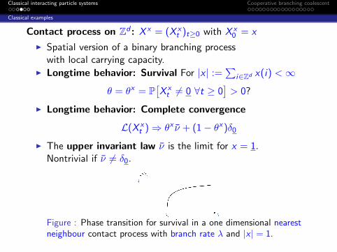
Contact process on Zd : X x = (X xt )t≥0 with X x
0 = x
I Spatial version of a binary branching processwith local carrying capacity.
I Longtime behavior: Survival For |x | :=∑
i∈Zd x(i) <∞
θ = θx = P[X xt 6= 0 ∀t ≥ 0
]> 0?
I Longtime behavior: Complete convergence
L(X xt )⇒ θx ν + (1− θx)δ0
I The upper invariant law ν is the limit for x = 1.Nontrivial if ν 6= δ0.
Figure : Phase transition for survival in a one dimensional nearestneighbour contact process with branch rate λ and |x | = 1.

Classical interacting particle systems Cooperative branching coalescent
Classical examples
Interacting particle system - dualities
Duality: E[1{|X x
t ·y |=0}]
= E[1{|x ·Y y
t |=0}], t ≥ 0
|x · y | =∑
i x(i)y(i).
For the contact process X ∼ Y (self-dual).
The above duality relates survival θδiX > 0 with nontriviality of νY :
E[1{|X x
t ·1|=0}]
= E[1{|x ·Y 1
t |=0}]
⇔ P[|X x
t · 1| 6= 0]
= P[|x · Y 1
t | 6= 0]
⇔ P[X xt 6= 0
]= P
[|x · Y 1
t | 6= 0]
With t →∞ and x = δi
θδiX = P[Y 1∞(i) 6= 0
]=
∫νY (dy)1{y(i)=1}.

Classical interacting particle systems Cooperative branching coalescent
Classical examples
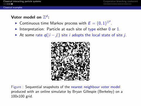
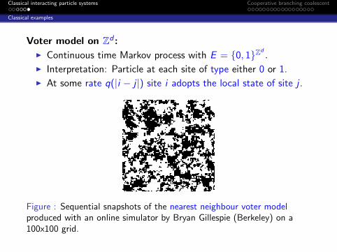
Voter model on Zd :
I Continuous time Markov process with E = {0, 1}Zd.
I Interpretation: Particle at each site of type either 0 or 1.
I At some rate q(|i − j |) site i adopts the local state of site j .
Figure : Sequential snapshots of the nearest neighbour voter modelproduced with an online simulator by Bryan Gillespie (Berkeley) on a100x100 grid.

Classical interacting particle systems Cooperative branching coalescent
Classical examples
Voter model on Zd :
I Continuous time Markov process with E = {0, 1}Zd.
I Interpretation: Particle at each site of type either 0 or 1.
I At some rate q(|i − j |) site i adopts the local state of site j .
Figure : Sequential snapshots of the nearest neighbour voter modelproduced with an online simulator by Bryan Gillespie (Berkeley) on a100x100 grid.
Classical interacting particle systems Cooperative branching coalescent
Classical examples
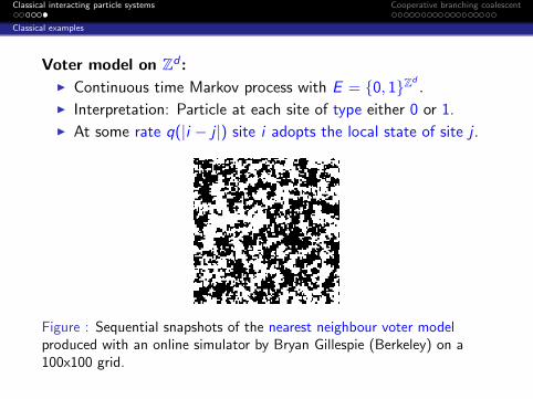
Voter model on Zd :
I Continuous time Markov process with E = {0, 1}Zd.
I Interpretation: Particle at each site of type either 0 or 1.
I At some rate q(|i − j |) site i adopts the local state of site j .
Figure : Sequential snapshots of the nearest neighbour voter modelproduced with an online simulator by Bryan Gillespie (Berkeley) on a100x100 grid.

Classical interacting particle systems Cooperative branching coalescent
Classical examples
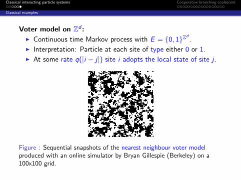
Voter model on Zd :
I Continuous time Markov process with E = {0, 1}Zd.
I Interpretation: Particle at each site of type either 0 or 1.
I At some rate q(|i − j |) site i adopts the local state of site j .
Figure : Sequential snapshots of the nearest neighbour voter modelproduced with an online simulator by Bryan Gillespie (Berkeley) on a100x100 grid.

Classical interacting particle systems Cooperative branching coalescent
Classical examples
Voter model on Zd :
I Continuous time Markov process with E = {0, 1}Zd.
I Interpretation: Particle at each site of type either 0 or 1.
I At some rate q(|i − j |) site i adopts the local state of site j .
Figure : Sequential snapshots of the nearest neighbour voter modelproduced with an online simulator by Bryan Gillespie (Berkeley) on a100x100 grid. Clustering occurs! Longtime coexistence?

Classical interacting particle systems Cooperative branching coalescent
Outline
1 Classical interacting particle systemsDefinitionClassical examples
2 Cooperative branching coalescentThe modelPhase transitionsParticle density and survival probability

Classical interacting particle systems Cooperative branching coalescent
The model
Cooperative branching coalescent (CBC)
Sturm and Swart: Annals of Applied Probability 2014
I Continuous time Markov process with state space {0, 1}Z:
X = (Xt)t≥0
I ”1” represents a particle, ”0” an unoccupied site.
I Symmetric random walk with coalescence:particles on adjacent sites merge at rate 1.
I Adjacent pairs of particles produce a new particle:particle is placed on a (randomly chosen) neighbouring site atcooperative branching rate λ.

Classical interacting particle systems Cooperative branching coalescent
The model
Motivation
As a model in the biological context:
1 Pair reproduction with migration and competition:”1” is a site occupied by an individual, ”0” is an empty site.Cooperative branching: pairs of individuals reproduce.Coalescing random walk: death due to competition.
2 Interface model of a multi type voter model:”1” is an interface between different ”types”.Cooperative branching: singletons give birth to a new type.Coalescing random walk: voter dynamics and disappearanceof types.
As a mathematical toy model:Tractable one dimensional model with interesting properties.

Classical interacting particle systems Cooperative branching coalescent
The model
The graphical representation
0 0 1 1 0 1 0
0 0 1 1 1 0 0
t
Z
t ∈ →ω(i)
cooperative branching
t ∈ →ω(i − 12 )
coalescing jump
For i ∈ Z→ω(i),
←ω(i) as well as
→ω(i − 1
2 ),←ω(i − 1
2 )
are Poisson processes with rate 12λ and 1
2 .

Classical interacting particle systems Cooperative branching coalescent
The model
Useful basic properties
The graphical representation provides a ”coupling” of processeswith different initial states and parameters.
I MonotonicityIf x ≤ y (componentwise) then the processes can be coupledsuch that
X xt ≤ X y
t for all t ≥ 0.
⇒ Monotoniciy in the initial states.
We also have monotonicity in λ.

Classical interacting particle systems Cooperative branching coalescent
The model
Simulation of the model
Simulation of a near-critical cooperative branching-coalescent withλ = 2 1
3 on a lattice of 700 sites with periodic boundary conditions,started from the fully occupied initial state.

Classical interacting particle systems Cooperative branching coalescent
Phase transitions
Long time behavior
I From monotonicity
P[X
1t ∈ ·
]=⇒t→∞
ν,
where ν is the upper invariant law.Probability under ν of finding a particle in the origin:
θ(λ) :=
∫νλ(dx)1{x(0)=1}
νλ is nontrivial if θ(λ) > 0.
I Survival probability of pairs - ”staying active”:
θ(λ) := P[|X δ0+δ1
t | ≥ 2 ∀t ≥ 0]
The process survives if θ(λ) > 0.
Classical interacting particle systems Cooperative branching coalescent
Phase transitions
Existence of phase transitions
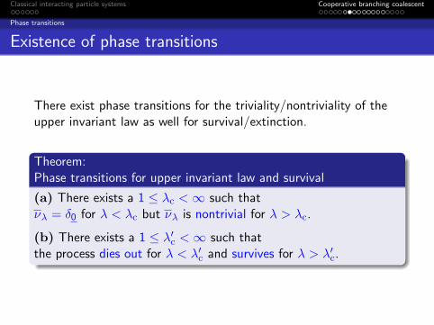
There exist phase transitions for the triviality/nontriviality of theupper invariant law as well for survival/extinction.
Theorem:Phase transitions for upper invariant law and survival
(a) There exists a 1 ≤ λc <∞ such thatνλ = δ0 for λ < λc but νλ is nontrivial for λ > λc.
(b) There exists a 1 ≤ λ′c <∞ such thatthe process dies out for λ < λ′c and survives for λ > λ′c.
Classical interacting particle systems Cooperative branching coalescent
Phase transitions
Existence of phase transitions
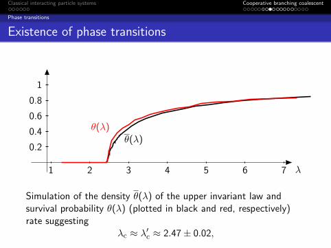
λ
θ(λ)θ(λ)
1 2 3 4 5 6 7
0.2
0.4
0.6
0.8
1
Simulation of the density θ(λ) of the upper invariant law andsurvival probability θ(λ) (plotted in black and red, respectively)rate suggesting
λc ≈ λ′c ≈ 2.47± 0.02,

Classical interacting particle systems Cooperative branching coalescent
Phase transitions
Proof ideas: Existence of phase transitions
Monotonicity implies the existence of λc and λ′c if we can show
(a) ν = δ0 for λ ≤ 1 and ν 6= δ0 for large λ.
(b) The process dies out for λ ≤ 1 and survives for large λ.

Classical interacting particle systems Cooperative branching coalescent
Phase transitions
Proof ideas: Existence of phase transitions
Triviality of the upper invariant law for λ ≤ 1: ν = δ∅
If λ > 0 and the process is started translation invariant letpt(1) = P(Xt(i) = 1), pt(11) = P(Xt(i) = 1,Xt(i + 1) = 1), . . . .
∂∂t pt(1) =−pt(1) + 1
2pt(10) + 12pt(01) + 1
2λpt(110) + 12λpt(011)
=−pt(11) + λ(pt(11)− pt(111)
)= (λ− 1)pt(11)− λpt(111),
If the process is furthermore started from an invariant law
0 = ∂∂t pt(1) ≤ −λpt(111)⇒ pt(111) = 0.
As pt(1) > 0 would imply pt(111) > 0 we are done.(Case λ = 0 similar.)

Classical interacting particle systems Cooperative branching coalescent
Phase transitions
Proof ideas: Existence of phase transitions
Extinction for λ ≤ 1: P[∃T <∞ s.t. |X x
t | = 1 ∀t ≥ T]
= 1.
With similar calculations
∂∂tE[|X x
t |]
= (λ− 1)∑i∈Z
P[X xt (i) = X x
t (i + 1) = 1]
−λ∑i∈Z
P[X xt (i) = X x
t (i + 1) = X xt (i + 2) = 1]
So |X xt | is a supermartingale for λ ≤ 1: |X x
t | −→t→∞N a.s.
⇒ N = 1 a.s.since if there were more particles left they would meet (a.s. due torecurrence) and interact (through branching or coalescence).

Classical interacting particle systems Cooperative branching coalescent
Phase transitions
Proof ideas: Existence of phase transitions
Nontrivial upper invariant law and survival for large λ :”Coupling” with another process: Pairs of adjacent particles arecoupled with a contact process variant.
The contact process with double deaths Y = (Yt)t≥0
I Sites infect any neighbor at rate 12λ.
I Any particles on two neighboring sites die at rate 1.
Graphical representation with Poisson processes:
←π(i − 1
2),→π(i − 1
2), and π∗(i − 1
2), i ∈ Z.

Classical interacting particle systems Cooperative branching coalescent
Phase transitions
Proof ideas: Existence of phase transitions
Nontrivial upper invariant law and survival for large λ :
Comparison of X with the contact process with double deaths Y
LetX
(2)t (i) := 1⇔ X x
t (i) = X xt (i + 1) = 1 t ≥ 0
denotes the locations of pairs of neighbouring particles in Xt . Then
(X(2)t )t≥0 and (Yt)t≥0 can be coupled such that
Y0 ≤ X(2)0 implies Yt ≤ X
(2)t t ≥ 0.
Coupling:
←π(i−1
2) :=
←ω(i),
→π(i−1
2) :=
→ω(i), π∗(i−1
2) :=
←ω(i−1
2)∪→ω(i+
1
2)

Classical interacting particle systems Cooperative branching coalescent
Phase transitions
Proof ideas: Existence of phase transitions
Comparison with oriented percolation
I By considering large times blocks we can can bound thecontact process with double deaths from below by orientedpercolation with arbitrarily large p for large enough λ.
I For large enough p the oriented percolation process has anontrivial upper invariant law and survives completing theproof.
Classical interacting particle systems Cooperative branching coalescent
Particle density and survival probability
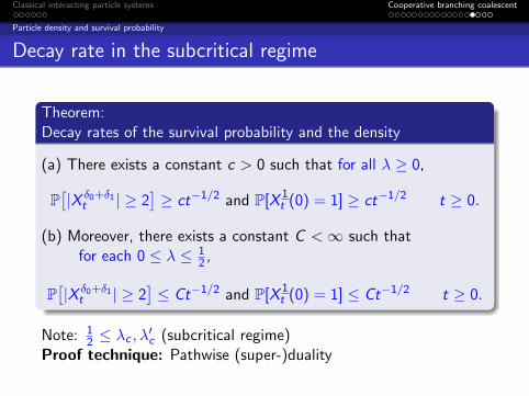
Decay rate in the subcritical regime
Theorem:Decay rates of the survival probability and the density
(a) There exists a constant c > 0 such that for all λ ≥ 0,
P[|X δ0+δ1
t | ≥ 2]≥ ct−1/2 and P[X
1t (0) = 1] ≥ ct−1/2 t ≥ 0.
(b) Moreover, there exists a constant C <∞ such thatfor each 0 ≤ λ ≤ 1
2 ,
P[|X δ0+δ1
t | ≥ 2]≤ Ct−1/2 and P[X
1t (0) = 1] ≤ Ct−1/2 t ≥ 0.
Note: 12 ≤ λc , λ
′c (subcritical regime)
Proof technique: Pathwise (super-)duality
Classical interacting particle systems Cooperative branching coalescent
Particle density and survival probability
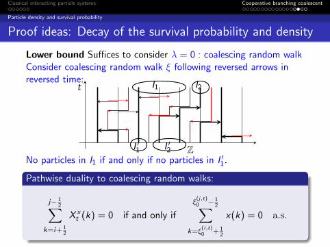
Proof ideas: Decay of the survival probability and density
Lower bound Suffices to consider λ = 0 : coalescing random walkConsider coalescing random walk ξ following reversed arrows inreversed time:
Z
t I1 I2
I ′1 I ′2No particles in I1 if and only if no particles in I ′1.
Pathwise duality to coalescing random walks:
j− 12∑
k=i+ 12
X xt (k) = 0 if and only if
ξ(j,t)0 − 1
2∑k=ξ
(i,t)0 + 1
2
x(k) = 0 a.s.

Classical interacting particle systems Cooperative branching coalescent
Particle density and survival probability
Proof ideas: Decay of the survival probability and density
Upper bound A pathwise superdual for λ > 0 (similar to Gray ’86)
Z
t I1 I2
I ′1 I ′2
Superduality: If there are particles in either I1 or I2 then theremust exist a ”backward 3-path” as drawn such that there areparticles in either I ′1 or I ′2. We can bound the expected numberof 3-paths over time t ”started” in adjacent sites.

Classical interacting particle systems Cooperative branching coalescent
Particle density and survival probability
Extensions of the model
Work in progress with Jan Swart and Tibor Mach:
I Include natural deaths.Exponential decay of particle density and survival
I Consider different graphs: Zd , trees, complete graph.Dual process for the mean field model
I Consider different sexes:Offspring only produced when parents are of opposite sex.Convergence to well mixed sexes andsimilar behavior to one sex model.
Thank you for your attention!