Longevity Risk Pricing*

Jiajia Cui†

Presented at the Living to 100 and Beyond Symposium

Orlando, Fla.

January 7-9, 2008

Copyright 2008 by the Society of Actuaries. All rights reserved by the Society of Actuaries. Permission is granted to make brief excerpts for a published review. Permission is also granted to make limited numbers of copies of items in this monograph for personal, internal, classroom or other instructional use, on condition that the foregoing copyright notice is used so as to give reasonable notice of the Society's copyright. This consent for free limited copying without prior consent of the Society does not extend to making copies for general distribution, for advertising or promotional purposes, for inclusion in new collective works or for resale. * An earlier version of the paper was presented during Living to 100: Survival to Advanced Ages International Symposium, Orlando, Jan. 7-9, 2008, the 16th international AFIR colloquium, Stockholm, June 2007 and the Netspar workshop in Maastricht on Nov. 23, 2006. The author is very grateful for the helpful comments by Frank de Jong, David Schrager, Roger Laeven, An Chen, Antoon Pelsser, Jianbin Xiao, Jeremie Lefebvre, Thaleia Zariphopoulou, Alexander Michaelides, Ron Anderson and Paula Lopes. † Tilburg University and ABP Pension Fund, the Netherlands; Postal Address: Department of Finance, Tilburg University, P.O.Box 90153, 5000 LE, Tilburg, the Netherlands. Phone: +31-13-4668206; Fax: +31-13-4662875. E-mail: j.cui@uvt.nl.

Abstract

Longevity risks, i.e., unexpected improvements in life expectancies, may lead to severe solvency issues

for annuity providers. Longevity-linked securities provide the desirable hedging instruments to annuity

providers, and in the meanwhile, diversification benefits to their counterparties. But longevity-linked

securities are not traded in financial markets due to the pricing difficulty. This paper proposes a new

method to price the longevity risk premia in order to tackle the pricing obstacle. Based on the equivalent

utility pricing principle, our method obtains the minimum risk premium required by the longevity

insurance seller and the maximum acceptable risk premium by the longevity insurance buyer. The

proposed methodology satisfies four important requirements for applications in practice: i) suitable for

incomplete market pricing, ii) accurate estimation of the risk premia, iii) consistent with other financial

market risk premia and iv) flexible in handling different payoff structures, basis risk and natural hedging

possibilities. The method is applied in pricing various longevity-linked securities (bonds, swaps, caps and

floors). We show that the size of the risk premium depends on the payoff structure of the security due to

the market incompleteness. Furthermore, we show that the financial strength of the longevity insurance

seller and buyer, the availability of the natural hedges and the presence of basis risk may significantly

affect the size of longevity risk premium.

1. Introduction

Longevity risks, i.e., unexpected improvements in life expectancies, impose a challenge on

pension plans and insurance companies because small unexpected improvement in life expectancies may

lead to severe solvency issues for these annuity providers. Longevity-linked securities are designed to pay

out more when a selected population group lives longer than originally expected. They are attractive

securities to financial markets because, on one hand, they are desirable assets for annuity providers to

hedge their longevity risks, and on the other hand, investors may find these securities attractive for the

benefits of diversification provided that the risk premia are set appropriately. Moreover, financial markets

may provide a more efficient risk allocation than the traditional insurance markets. Although academic

researchers, policy makers and practitioners have talked about it for years, longevity-linked securities are

not traded in financial markets due to the pricing difficulty. This paper therefore proposes a new method

to price the longevity risk premia in order to tackle the pricing obstacles of the innovative longevity-

linked securities.

This paper contributes to the literature by quantifying the longevity risk premia in various

longevity-linked securities (bonds, swaps, caps and floors), applying the equivalent utility pricing

principle. Based on the equivalent utility pricing principle, we obtain a minimum risk premium required

by the longevity insurance seller and a maximum acceptable risk premium by the longevity insurance

buyer. These upper and lower bounds indicate a price range for negotiation between the sellers and the

buyers. The four main advantages of our methodology are: i) the suitability for incomplete market

pricing, ii) a narrow range of the risk premia, iii) the consistency with other financial market risk premia

(like inflation risk premium) and iv) its flexibility in handling different payoff structures, basis risk and

natural hedging possibilities.

In practice, life insurers, also pension funds, claim that their annuity businesses are losing money

due to the unexpected longevity improvements over years. In the past centuries remarkable improvements

in human life expectancy have been observed. The uncertainties about the further improvements of

human life expectancy are referred to as the longevity risks. Oeppon and Vaupel (2002, in Science) report

striking evidences that the record life expectancy has been rising nearly three months per year in the past

160 years, and the asserted ceilings on life expectancy were surpassed repeatedly in the past century. In

fact, the future improvements of life expectancy are difficult to be predicted accurately.‡ The general

opinion from the experts tends to be that the trend of longevity improvements is certain, but deviations to

both sides are possible.

‡ Brown and Orszag (2006) discuss the difficulties in making an accurate mortality projection.

Reinsurance contracts do exist, but the capacity of reinsurance is limited (OECD (2005)). By a

reinsurance contract, the longevity risk is concentrated on one large reinsurance company. The

reinsurance approach works best when the underlying risks are diversifiable. However, the fact that

longevity risk is a systematic risk weakens the diversification principle that the reinsurance requires.

Longevity risk cannot be reduced by diversification or increasing the size of the pool.§

Alternatively, the longevity risk could be transferred to financial markets, also known as

securitization. By transferring longevity risk to financial markets, the risk is distributed among a (large)

number of market participants who can shoulder the risk better, i.e., achieving more efficient risk

allocation. Longevity-linked securities are one of the current financial market innovations. The first

longevity bond was announced by the EIB and BNP** Paribas in November 2004, but it has been under-

subscribed, and withdrawn for redesign in late 2005.†† The EIB/BNP survivor bond is a coupon-based

bond, with floating annual coupons linked to a cohort survivor index. The problem with this issuance is

that there is no clear view on how longevity risk should be charged. The EIB/BNP survivor bond required

a longevity risk premium of 20 basis points, which was regarded as too high for some annuity providers.

The EIB/BNP bond, although linked to the British survivor index, was also marketed among Dutch

pension funds. However, it was not clear for the Dutch pension funds whether the 20 basis points was a

good deal or not.

The origin of the pricing difficulty lies in the fact that the financial market is incomplete when

longevity securities are not traded. Therefore, the goal of this paper is to provide a pricing framework

suitable for pricing longevity risks in incomplete market setting. Based on the equivalent utility pricing

principle, our method obtains the minimum risk premium required by the longevity insurance seller and

the maximum acceptable risk premium by the longevity insurance buyer. We find that the size of the risk

premium depends on the payoff structure of the security, the financial strength of the seller and the buyer

and the availability of the natural hedge. We show that different payoff structures and maturities may lead

to different risk premia because the market is incomplete. We also show that financially stronger issuer

may require a lower risk premium. Furthermore, the risk premium could be reduced by distributing the

longevity risk among more market participants. The market calls for more longevity bond issuers in order

to achieve more efficient allocation and reduce the longevity risk premium. One important implication for

§ We must differentiate mortality risk from longevity risk. Mortality risk refers to the uncertainty about individual death events when the life expectancy is known. Therefore, mortality risk is a micro risk, and can be diversified by increasing the size of the pool. ** EIB/BNP stands for the European Investment Bank (EIB) and Banque Nationale de Paris (BNP). †† Blake, Cairns and Dowd (2006) address the associated obstacles in current market development of longevity-linked securities. The obstacles are categorized into `design issues' (regarding the payoff structure, maturity, choice of survivor index, nominal or real payments, etc.), `pricing issues' and `institutional issues'. As to the pricing issues, the authors comment that "even if the (survivor) bond provides a perfect hedge, there will be uncertainty over what the right price to pay or charge should be."

the market development of longevity-linked securities is that multiple sellers, instead of a single seller,

are required.

In this paper, the longevity risk is modeled as proposed by Lee and Carter (1992), and estimated

according to the U.K. and the Dutch mortality data. However our pricing methodology is quite general.

Other stochastic mortality models are also suitable for our pricing framework.

Recently, a few approaches to price longevity risk were proposed in the literature. Friedberg and

Webb (2005) apply Capital Asset Pricing Model (CAPM) and Consumption-based Capital Asset Pricing

Model (CCAPM) to estimate the longevity premium. Their result based on CAPM leads to a risk

premium of 75 basis points, with confidence interval ranging from -75 to 230 basis points, due to

inaccuracy in estimating the beta. Their result based on CCAPM is merely two basis points, due to the

low variation in consumption data. The discrepancy between the author claimed two basis points and the

market claimed 20 basis points is similar to the equity premium puzzle using the CCAPM approach.

Milevsky, Promislow and Young (2005, 2006) proposed a Sharpe ratio approach, which is based on mean

and volatility of payments instead of returns. The methodology used in this paper is the equivalent utility

pricing principle. Our approach is suitable for pricing in incomplete market. It provides a narrow price

range for negotiation. The resulting risk premia are consistent with other financial market risk premia

(like inflation risk premium). Our pricing framework is flexible in handling different payoff structures,

basis risk and natural hedging possibilities.

Apart from securitization, there are three other possibilities of managing longevity risk, namely

hedging, reserving and risk sharing.‡‡ The longevity risk could be partly hedged using natural hedging, for

example between life annuity and term insurance. This paper illustrates the effect of the natural hedging

on longevity risk premia. The impact of natural hedging is potentially significant.

The organization of this paper is the following: Section 2 introduces stochastic mortality models

in order to quantify longevity risks. Section 3 describes longevity-linked securities, and incomplete-

market pricing principles. In Section 4 we quantify the (seller's minimum) longevity risk premium for

EIB/BNP type of longevity bonds using the equivalent utility pricing principle. Section 5 extends the

longevity risk premia calculation to other longevity linked securities, including swaps, deferred bonds,

floors and caps. Section 6 introduces the possibility of natural hedging into our pricing framework.

Section 7 considers buyer's maximum premium, together with the presence of basis risk. Section 8

concludes.

‡‡ See also Brown and Orszag (2006), Blake, Cairns and Dowd (2006).

2. Stochastic Mortality Models and Longevity-Linked Securities This section first presents a stochastic mortality model to quantify longevity risks, and then

describes the longevity-linked securities in more details.

2.1. Stochastic Mortality Models The literature of stochastic mortality trend starts from Lee and Carter (1992).§§ According to

Deaton and Paxson (2004), the Lee-Carter model has become the `leading statistical model of mortality in

the demographic literature'. Therefore, the numerical results presented in this paper are based on Lee and

Carter (1992) model.

Other stochastic mortality models may also fit well in our pricing framework. Dahl (2004) and

Schrager (2006) advocate the affine stochastic mortality models to capture the birth cohort mortality

dynamics over one's life cycle instead of the time series of an age group over time. We leave the affine

stochastic mortality approach as a future work for robustness analysis.

Lee and Carter (1992) model the time series behavior of log central death rate of an age group by

using a single latent factor. The latent factor drives the mortality rates of all age cohorts. Formally, the log

mortality rate of the x-year-old, ( )( )tx,ln μ , is determined by a common latent factor, tγ , with an age-

specific sensitivity parameter, xβ , and an age-specific level parameter, xα ,

( ) txtxxtx ,,ln δγβαμ ++= (1)

where transitory shocks ( )2, ,0~ δσδ Ntx are white noises. And tγ satisfies a random walk with drift

process as

ttc εγγ ++= −1t (2)

where permanent shocks ( )2,0~ εσε Nt are white noises. tx,δ and tε are independent.

Assuming that the force of mortality is constant during a year txutux ,, μμ =++ (0 ≤ u <1), the

survival probability at time t of the x-year-old over one-year horizon is given by

( ) ( ) ( )txtxx tptp ,][ exp0

μ−== + . Similarly, the conditional probability at time t of an x-year-old surviving

next τ years is given by

( ) ⎟⎠

⎞⎜⎝

⎛−= ∑

=++

τ

τ μ1

,expi

itixx tp (3)

§§ Various extensions of the Lee-Carter model can be found in Cairns, Blake and Dowd (2005b), Hari, De Waegenaere, Melenberg and Nijman (2006).

We estimate this model using the yearly U.K. (England and Wales) and Dutch male mortality

data from 1880 to 2003, downloaded from the Human Mortality Database.*** Appendix A provides a

more detailed treatment of the model, together with its estimation and simulation procedures. The

estimated latent process (in the United Kingdom) is the following, including two temporary shocks

captured by a `WWI' dummy and a `WWII' dummy†††:

ttt WWII εγγ ++++−= − *9.1WWI*0.650725.0 t1t (4)

with the volatility 169.0=εσ . The dummy variables do not change the drift but reduce the volatility of

the innovations. The estimation results using the Dutch data are reported in Appendix A.

FIGURE 1: The estimated Lee-Carter (1992) model parameters, with xβ (left upper panel), tγ (right upper panel), xα (left lower panel) and ( )( )tx,ln μ (right lower panel, the top curve for age

x = 65, and the bottom dashed curve for x = 35).

0 20 40 60 80 1000

0.1

0.2

0.3

0.4

0.5beta (U.K.)

age1900 1950 2000

-6

-4

-2

0

2

4

6gamma (U.K.)

year

0 20 40 60 80 100-8

-6

-4

-2

0alpha (U.K.)

age1900 1950 2000

-7

-6

-5

-4

-3

-2log(μ), x=35 and 65, U.K.

year

*** Human Mortality Database University of California, Berkeley (USA), and Max Planck Institute for Demographic Research (Germany). Available at www.mortality.org or www.humanmortality.de (data downloaded on March 27, 2006). ††† The `WWI' dummy takes non-zero values for years {1914 =1.5; 1915 = 1.5; 1916 = 1; 1917 = 1; 1918 = 1; 1919 = -4; 1920 = -2} and zero elsewhere. The `WWII' dummy takes non-zero value for years {1940 = 1; 1944 = 0.1; 1945 = 0.1; 1946 = -1.2} and zero elsewhere.

FIGURE 2 (a): The forecasted force of mortality ( )tx,μ (left panel) and the forecasted survival probabilities xpt (right panel) of the 65-year-old cohort retiring in year 2004.

FIGURE 2 (b): The standard deviation (left) and skewness (right) of the simulated survival probabilities, 65t p .

Assuming that the estimated model (4) is the `true’ process, and taking the estimated parameters

as of year 2003, we could simulate the latent process tγ and the resulting survival probabilities of the 65-

yaer-old male cohort from year 2004 onwards. Figure 2(a) describes the distribution of a set of simulated

survival probabilities of the 65-year-old male. From Figure 2(b) we see that the volatility of the survival

probabilities exhibits a hump shape, which means that the uncertainty over a longer horizon (up to 20

years) first increases and then decreases. The distribution is also skewed. The skewness increases with

age.

Using the estimation results, we can show the size of the uncertainties involved in life expectancy

and annuity prices. The expected remaining life time of an x-year-old at time t is given by

[ ] ( )⎥⎦

⎤⎢⎣

⎡= ∑

−

=

x

xtt tpETEω

ττ

1 (5)

where ω denotes the maximum obtainable age, e.g., ω = 110. The price of an immediate annuity paying 1

euro in each surviving year, assuming a fixed and flat yield curve r, is given by

[ ] ( )⎥⎦

⎤⎢⎣

⎡= ∑

−

=

−x

xrt

tt tpeELE110

1ττ (6)

According to the estimated Lee-Carter model, the remaining lifetime of a 65-year-old British

male in year 2004, is 16 years with standard error of [± 0.2] years, as given by (5). An immediate annuity

paying 1 euro in each surviving year on average worthies‡‡‡ 13.1 euro, assuming a fixed and flat yield

curve at r=2%, as given by (6). The standard error of the value of this annuity is [± 0.15] euro, or [±

1.1%] in relative terms. The longevity risk in these immediate annuities is not negligible.

2.2. Longevity-Linked Securities Given the potential size of the longevity trend uncertainty, financial markets proposed longevity-

linked securities. The first longevity bond was announced by the EIB and BNP Paribas in November

2004, but withdrawn for redesign in late 2005. The EIB/BNP bond is a `coupon-based' bond, in which the

notional annual coupon is indexed to a cohort survivor index in England and Wales. This cohort retires at

age 65 in 2004. The maturity of this bond is 25 years. Section 4 discusses the pricing of such bonds.

Blake, Cairns and Dowd (2006) address the lessons learned from the failure of the EIB/BNP survivor

bond and provide constructive suggestions for future developments of the flourishing new market. The

main lessons are the following:

1) The designed 25-year horizon is perhaps too short for an effective hedge, since longevity risk

in the near future (<10 years) is small.

2) The up-front capital requirement is large, especially since a major part of the capital is taken by

the ineffective hedge coupons in the near future.

3) The coupons are indexed to 65-year-old males, but annuity providers worry about longevity

risk of younger cohorts and females.

4) There is large uncertainty about what the right price is that should be charged.

5) Hedge failure or basis risks are large, due to a number of reasons: the reference population is

different from that of an annuity provider; the survivor index is not timely available, etc.

6) The payments are nominal, whereas most pension schemes aim at inflation-linked real

payments.

‡‡‡ Money's worth of annuity is the expected discounted value of future payments, without risk loadings.

Their paper also introduces a few innovative hypothetical mortality-linked securities as potential

solutions to the aforementioned problems. These securities include Zero-Coupon Longevity Bonds,

Longevity Bull Spread Bonds, Deferred Longevity Bonds, Vanilla Mortality Swaps, Survivor Caps and

Floors, Mortality Swaptions and Longevity Future. Enlightened by these discussions, this paper presents

the required longevity risk premia in different longevity-linked security designs, including zeros,

EIB/BNP bonds, swaps, caps and floors and deferred longevity bonds. This paper also considers the

impacts of natural hedge and basis risk in Sections 6 and 7.

3. Longevity Risk Pricing Principles, a Review This section reviews the recent literatures on incomplete market pricing, and motivates our choice

of the methodology. Finally, we specify the utility preference needed for the equivalent utility pricing

principle.

CAPM- and CCAPM-based approach. Friedberg and Webb (2005) apply Capital Asset

Pricing Model (CAPM) and Consumption-based Capital Asset Pricing Model (CCAPM) to estimate the

premium for longevity risk. The authors construct a pseudo-EIB/BNP survivor bond. Let tbR , denote the

returns of such pseudo survivor bonds. Following the CAPM, the longevity risk premium is its beta,

which is defined by ( ) 2b /,cov mmb RR σβ = , times the market risk premium:

( ) ( )[ ]fmbfbt RRERRE −=− β

The authors claim that the beta on pseudo-EIB/BNP bond is 0.15 with 95 percent confidence

interval of [-0.15, 0.46]. Therefore, if market risk premium is 5 percent, the longevity risk premium on

this bond is 75 basis points, with confidence interval of [-75, 230] basis points. Given the wide

confidence interval, the authors suggest that CCAPM as a better alternative.

Following the CCAPM, the longevity risk premium is determined by the relationship between the

expected return on the asset and the marginal utility of consumption.

( ) ( )( )( )( )1

1,11, '

,'

+

+++ −=−

tt

tbttftbt CUE

RCUCovRRE

The paper shows that the correlation between consumption growth and survivor bond returns is -

0.1958 and is significant. However, since the standard deviation of mortality bond returns is small, as a

result, the covariance between survivor bond returns and consumption growth is extremely small at -

0.0015 percent. Applying the CCAPM, the risk premium is only two basis points when the coefficient of

risk aversion equals 10. This result is far below the 20 bp risk premium marketed in the EIB/BNP bonds.

Sharpe ratio approach. Cochrane and Saa-Requejo (2000) suggest that the absolute value of

the Sharpe ratio on any unhedgeable portfolio should be bounded, so that too `good deals' are ruled out.

Milevsky, Promislow and Young (2005, 2006) propose a so-called instantaneous Sharpe ratio to

determine the mortality risk premia. Using the analogy to the Sharpe ratio in the financial market, which

is the ratio of the expected excess return and the return volatility [ ]( ) [ ]RRRESR fMarket σ/−≡ , the

Sharpe ratio in the insurance context could be defined as the excess payoff above the expected payment,

divided by the standard deviation of the risky payment, ( ) [ ]( ) [ ]NNInsur WWELNSR σ/1 −+≡ . The

authors argue that the longevity risk loading L will be set so that the Sharpe Ratio is consistent with other

asset classes in the economy. For example, if the Sharpe ratio for large cap equities is roughly 0.25, then

the Sharpe ratio of the insurance policy should also be bounded within a similar magnitude.§§§

Equivalent utility based approach. The pricing method proposed in this paper is based on the

equivalent utility pricing principle. The equivalent utility based approach is a popular pricing

methodology for incomplete market setting. The related literature includes Svensson and Werner (1993),

Young and Zariphopoulou (2002), Young (2004), Musela and Zariphopoulou (2004), De Jong (2007),

Chen, Pelsser and Vellekoop (2007) and other references listed in the bibliography. As pointed out by

Svensson and Werner (1993), the shadow value of a non-traded or non-hedgeable asset (the price of

longevity risks in this case) can be interpreted as an additional amount of wealth added to the investor's

budget so that the investor is indifferent between holding a non-hedgeable asset and hedgeable asset.

Furthermore, the shadow value is investor-specific, depending on the investor's preference. In the context

of longevity-linked securities, equivalent utility pricing principle reveals the minimum compensation

required by the seller and the maximum price acceptable to the buyer. Therefore, this paper shows the

range of possible prices for the longevity-linked securities before the market opens up.

De Jong (2007) applies the principle of equivalent utility in pricing wage-linked securities, in an

incomplete market setting. In the context of defined benefit pension fund liability valuation, the main

source of unhedgeable risk is the real wage growth. The pension fund is modeled as a potential buyer of

the wage-linked bonds. Hence the equivalent utility pricing gives the maximum risk premium that the

pension fund is willing to pay in order to obtain the insurance against the wage rate fluctuations. The

paper shows the risk premium is determined by the additional wealth needed to be invested in the

§§§ The authors are still working on the estimation of the Sharpe ratio using annuity rate quotes. The results are not available yet.

financial market in order to provide the participants the same level of utility as a fully wage-indexed

pension.

Assuming exponential utility function, Musela and Zariphopoulou (2004), as well as Henderson

(2002), show a simple analytical formula for pricing an non-traded claim. As we shall see, the pricing

formula of the longevity-linked claims derived in this paper is consistent with the result found by above

mentioned authors. The next sub-section illustrates the idea of equivalence pricing principle using a very

simple model. The complete model is treated in Section 4.

3.1. An Application Before going into the pricing, let us fix some notations. In the context of annuities, let N denote

the initial size of the x-year-old cohort at time zero, and K is the agreed amount of annuity payment per

annual. In the context of longevity bonds with varying coupons, NK denotes the notional coupon, and

xt pNK is the actual amount of coupon due in year t. In this paper, K is normalized to 1. Finally, the

number of survivors in this cohort in year t is given by xtt pNKS = . The survival index in t years' time is

a random variable, with mean [ ]tSE , and variance [ ]tSVar . We assume that the longevity risk is the

only risk factor in this simple illustration.

Now we illustrate the equivalent pricing principle by pricing a zero coupon longevity bond, with

maturity of t years. Such zero coupon bond is effectively a large group of single premium endowment

contracts which pays an agreed amount (normalized to K = 1) at a future time t to the survivors of the

current x-year-old cohort. The longevity risk can be described as the deviation from the expected survival

rate, [ ]tt SES − . Let's call the longevity bond issuance company (or the pure endowment seller) the

`seller', since the `seller' provides insurance against longevity risk. The single premium is paid at time

zero, and consists of two parts. One part is the expected loss [ ]tSE and the other part is a risk premium

loading P.

The seller invests her initial wealth 0W and the received total premium in risk free asset. Further

assume that the risk free rate is zero, hence, 0WWt = . The minimum premium loading for this single

premium endowment contract is the lowest amount that the seller asks for bearing the longevity risk

[ ]tt SES − . Thus, the minimum premium loading, denoted as −P , equalizes the expected utility of

underwriting the risk tS with a compensation [ ] −+ PSE t , with the utility of not underwriting the risk,

from the seller's viewpoint. Let U(⋅) denote the utility function of the seller, we have

[ ]( )[ ] ( )tttt WUSPSEWUE =−++ −

Case 1: Constant Absolute Risk Averse (CARA) utility

First we assume the seller has a CARA preference, ( ) ( )wwU αα

−−= exp1, where α is the

absolute risk aversion coefficient.

[ ]( )[ ] ( )tttt WSPSEWUE αα

−−=−++ − exp1

The resulting risk loading is given in expression (7), which is also known as the exponential risk

premium (Kaas, et al. (2001), p. 7).

[ ]( )( )[ ]tt SSEEP −=− αα

expln1 (7)

The total premium can be seen as the `best estimate' plus the (macro) risk premium which equals

the logarithm of the moment generating function of risk tS at argument α divided by the CARA

coefficient α . Notice that the risk loading is not affected by the initial wealth, 0W , for the CARA

preference.

In a special case, if tS is normally distributed, then the minimum loading −P is proportional to

the variance of tS , as given in expression (8. However, Figure 2(b) shows that the distribution of tS is

skewed. Therefore the handy expression (8) is not an accurate approximation.

[ ] [ ]( )[ ]( ) [ ]( )

[ ]( )( )[ ] [ ]⎟⎠⎞

⎜⎝⎛=−

−

ttt

ttt

ttt

SVarSSEE

SVarNSESthen

SVarSENSif

2

2

21expexp

,0~

,~

αα

αα

[ ]tSVarP α21

=− (8)

Case 2: Constant Relative Risk Averse (CRRA) utility

Alternatively we assume the seller has a CRRA utility: ( ) ( )γγ −= − 1/1wwU . Notice that the risk

loading does depend on the initial wealth and risk aversion parameter for the CRRA preference. The

minimum loading −P is the one that solves equation (9).

[ ]( )[ ] ( )γγ −=−++ −− 1/1tttt WSPSEWUE

[ ] 11

1

=⎥⎥⎦

⎤

⎢⎢⎣

⎡⎟⎟⎠

⎞⎜⎜⎝

⎛ −++

−− γ

t

tt

WSPSEE (9)

Numerical results:

The risk loading −P of both cases can be evaluated by means of simulation. Using the estimation

and simulation procedures presented in Appendix A, we calculate the expected loss [ ]tSE and the risk

loading −P for the endowment contract. The total premium paid per person is [ ]( ) NPSE t /−+ . We can

express −P in terms of risk premium, pR , which is a discount rate above the risk free rate (i.e. 0 percent

as assumed) and an actuarial discount rate aR :

( ) [ ]N

PSERR tt

pa

−− +=++1

where the actuarial discount rate aR is defined by

( ) [ ] [ ]xttt

a pENSE

R ==+ −1

The risk premia for CARA and CRRA utility specifications are presented in Tables 1 and 2

below.

TABLE 1: The longevity risk premium pR in basis points, for different cohort sizes (N = 10, 100, 1000 ×10³) and different risk aversion values (CARA(α) = 1,3,5).

N = 10 N = 100 N = 1000

maturity CARA = 1 CARA = 3 CARA = 5 CARA = 1 CARA = 3 CARA = 5 CARA = 1 CARA = 3 CARA = 5

5 0 0 0 -1 -2 -3 -5 -12 -15 10 0 -1 -1 -2 -7 -11 -18 -24 -26 15 -1 -2 -3 -6 -16 -24 -31 -38 -39 20 -1 -3 -5 -10 -28 -39 -48 -55 -57 25 -1 -4 -6 -13 -37 -54 -70 -82 -85 30 -1 -3 -4 -9 -27 -46 -78 -104 -109 35 0 -1 -1 -3 -9 -15 -31 -91 -112

TABLE 2: The longevity risk premium pR in basis points, for different cohort sizes (N = 10, 100, 1000

×10³) and different risk aversion values (CRRA(γ) = 3,5,8). The initial wealth of the insurer is assumed to be 0W = 100.

N = 10 N = 100 N = 1000

maturity CRRA =

3 CRRA =

5 CRRA =

8 CRRA =

3 CRRA =

5 CRRA =

8 CRRA =

3 CRRA =

5 CRRA =

8

5 0 0 0 0 0 0 0 0 0 10 0 0 0 0 0 0 -1 -1 -2 15 0 0 0 0 0 0 -2 -3 -5 20 0 0 0 0 -1 -1 -3 -5 -8 25 0 0 0 0 -1 -1 -4 -6 -10 30 0 0 0 0 0 -1 -3 -4 -7 35 0 0 0 0 0 0 -1 -1 -2

The key features of the results are: 1) The required risk premium is negative, meaning that the

bond yield is lower than the risk free rate, so that the bond price is higher than the risk free bond. Thus,

the insurer (i.e., the survivor bond issuer) is compensated for bearing longevity risks. 2) The additional

discount rate pR (in absolute value) increases as the size of the pool increases. 3) The more risk averse

the insurer is, the higher compensation is required. 4) Approximately, the longer the maturity, the higher

compensation is required.

3.2. Preference Assumption The results in Tables 1 and 2 reveal some unsatisfied properties of CARA and CRRA

preferences. For a CARA investor, he has the same worry about one additional euro loss no matter how

rich or poor he is. For a CRRA investor, he cares much less when he is rich. In our view, both preferences

are too restrictive to characterize the risk preference of financial institutions. The CARA utility might

overestimate the longevity risk premium, whereas the CRRA utility might underestimate the risk

premium. Therefore, we modify the CARA utility, to make the risk aversion depend on the initial capital

or initial wealth of the company, ( ) bWW −= 00 αα where b∈[0,1]. In general, risk aversion decreases

with initial wealth.****

At the two extremes, the modified utility approaches CRRA specification when b = 1, and the

modified utility is back to the CARA specification when b = 0. The proposed preference (10) retains

some convenient features of the negative exponential utility function. The expected utility is separable for

independent risks x and y, since ( )[ ] ( )[ ] ( )[ ]yExuEyxuE α−=+ exp .

( ) ( ) ( )( )SWW

Su 00

exp1 αα

−−= (10)

It is important to be clear about whose preference that (10) captures. Sections 3 to 5 focus on

seller's minimum required risk premium. Therefore the utility function (10) represents the preference of

the shareholders of the seller. In the context of the EIB/BNP longevity bond, it is the preference of the

shareholders of EIB/BNP. Section 6 discusses the buyer's maximum risk premium. Hence the utility

function (10) represents the preference of the buyer, e.g., a pension fund.

**** Wachter and Jogo (2007) (and their references) provide arguments and evidences for a wealth-varying risk aversion.

4. Pricing of a Coupon-Based Longevity Bond This section derives the minimum required longevity risk premium of a coupon based longevity

bond from the seller's point of view. The longevity bond is linked to a large pool of population. Therefore

mortality risk (also called micro longevity risk) is fully diversified. The setup of the model is the

following. The shareholder of a financial company (like EIB/BNP) derives her utility from dividends and

final wealth. We consider two alternative situations. In the first situation, the company does not insure

longevity risk, hence is not exposed to longevity risk. In the second situation, the company issues a

longevity bond and hence bears longevity risk. Furthermore, we assume that the macro longevity risk is

independent from the financial risks. The methodology used in this section combines the martingale

approach with the equivalent utility pricing principle.

4.1. Setup Problem 1 without longevity risk

Assume a complete financial market, with constant risk free rate, r. The shareholder (or manager)

of the company derives her utility from dividends and final wealth at the end of the horizon, T. The per-

period utility is described as (10), and δ is the subjective discount rate of the shareholders. The initial

equity capital of the company is given by 0W . The company maximizes the shareholder's utility by

optimizing asset allocation ( tx ) and dividend ( tD ) decisions. Formally the optimization problem is the

following

( ) ( )⎥⎦⎤

⎢⎣⎡ += −−∫

=T

TT

tt

WDxWuedtDueEV

TTttt

δδ

00,},{ 0

max (11)

s.t. 00WWMdtDME TT

T

tt =⎥⎦⎤

⎢⎣⎡ +∫ (12)

where tM is the pricing kernel for the complete financial market. In our model, tM is given by

ttt dZrdtMdM λ−−=/ (13)

Problem 2 with longevity risk

In the same financial market, the company issues coupon-based longevity bond, in which the

annual coupon is indexed to the 1939-born cohort survivor index. This cohort retires in 2004 at age 65.

The longevity risk is not hedgeable from the financial market. Hence, the company derives her utility

from dividends and the residual claim ( [ ] tt SSE − ) from the longevity risk. The initial equity capital of

the company is now augmented by an additional risk loading π. The company maximizes her utility by

optimizing asset allocation and dividend decisions. Formally the optimization problem is the following

[ ]( ) ( )⎥⎦⎤⎢⎣⎡ +−+= −−∫

=

πδπδπππ T

TT

tttt

WDxWuedtSSEDueEV

TTttt

00,},{ 0

max (14)

s.t. πππ +=⎥⎦⎤

⎢⎣⎡ +∫ 00

WWMdtDME TT

T

tt (15)

Applying the equivalent utility pricing argument, we determine the minimum risk compensation π

such that the company is indifferent from bearing the longevity risk and without the longevity risk. That

is, the indirect utility must be equal under these two situations:

π00 VV = (16)

4.2. Results The derivations are given in Appendix B. The main results are the following: The risk loading π

is a present value of the certainty equivalent compensations for the risks [ ] tt SSE − , as given by (17).

[ ]( )( )[ ]

∫

∫−

−

=

−−=

T

trt

T

ttrt

dtGe

dtSSEEe

0

0

ln1

expln1

α

αα

π (17)

where α is the shorthand notation for ( ) bWW −= 00 αα , and

[ ]( )( )[ ]ttt SSEEG −−= αexp (18)

The value of the coupon-based longevity bonds with maturity T can be decomposed into 'best

estimated' price [ ]∫ −T

trt dtSEe

0 and longevity risk loading (π):

Total price = best estimate + risk loading = [ ] π+∫ −T

trt dtSEe

0 (19)

Table 3 shows the normalized risk loading, (π/(beste stimate)), of the coupon-based longevity

bonds with maturity T = 5,...,35 years. The risk loading depends on the maturity of the bond, the size of

initial equity capital and the risk aversion of the insurer. Recall that the risk aversion is inversely related

to the size of the capital, as ( ) bWW −= 00 αα . As b changes from 1 to 0, the preference shifts from CRRA

to CARA, resulting in the increases in risk loadings. CRRA investor requires virtually zero risk

compensation. Whereas CARA investor requires a sizable compensation, up to 1.6 percent of the best

estimated cost.

We can also express the risk loading π in terms of risk premium, pR , which can be seen as an

additional discount rate above the risk free rate to adjust for the longevity risk. As explained in Section

3.1, the risk premium is negative, meaning that the bond yield is lower than the risk free rate, so that the

bond price is higher than the risk free bond. Thus, the insurer (i.e., the survivor bond issuer) is

compensated for bearing longevity risks.

total price = [ ] π+∫ −T

trt dtSEe

0 = ( ) [ ]∫ +−T

ttRr dtSEe p

0

Or, per policy： [ ] ( ) [ ]∫∫ +−− =+T

ttRrT

trt dtpEeNdtpEe p

0 650 65 /π .

TABLE 3: The normalized risk loading per person, π/best estimate, of EIB/BNP longevity bonds for different sizes of the initial equity capital, 0W = [10000,1000,100] million, and different risk aversion

specifications ( ) bWW −= 00 αα , with α = 3, b = [1,(1/4),(1/8),0]. The size of the insured pool is N = 100 million, K = 1.

equity w0 = 10000 w0 = 1000 w0 = 100

maturity b=1 b=1/4 b=1/8 b=0 b=1 b=1/4 b=1/8 b=0 b=1 b=1/4 b=1/8 b=0

5 0% 0% 0,0% 0,0% 0% 0,0% 0,0% 0,0% 0% 0,0% 0,0% 0,0%

10 0% 0% 0,1% 0,2% 0% 0,0% 0,1% 0,2% 0% 0,1% 0,1% 0,2%

15 0% 0% 0,2% 0,5% 0% 0,1% 0,2% 0,5% 0% 0,2% 0,3% 0,5%

20 0% 0% 0,3% 0,9% 0% 0,2% 0,4% 0,9% 0% 0,3% 0,6% 0,9%

25 0% 0% 0,4% 1,4% 0% 0,3% 0,6% 1,4% 0% 0,4% 0,8% 1,4%

30 0% 0% 0,5% 1,5% 0% 0,3% 0,7% 1,5% 0% 0,5% 0,9% 1,5%

35 0% 0% 0,5% 1,6% 0% 0,3% 0,7% 1,6% 0% 0,5% 0,9% 1,6%

TABLE 4: The longevity risk premium pR (in basis points) of EIB/BNP longevity bonds for different

sizes of the initial equity capital, 0W = [10000,1000,100] million, and different risk aversion parameters

( ) bWW −= 00 αα , with α = 3, b = [1,(1/4),(1/8),0]. The size of the insured pool is N = 100 million, K = 1. equity w0 = 10000 w0 = 1000 w0 = 100

maturity b=1 b=1/4 b=1/8 b=0 b=1 b=1/4 b=1/8 b=0 b=1 b=1/4 b=1/8 b=0

5 0 0 0 -1 0 0 0 -1 0 0 -1 -1

10 0 0 -1 -3 0 -1 -1 -3 0 -1 -2 -3

15 0 -1 -2 -7 0 -1 -3 -7 0 -2 -4 -7

20 0 -1 -4 -11 0 -2 -5 -11 0 -4 -7 -11

25 0 -2 -5 -15 0 -3 -6 -15 0 -5 -8 -15

30 0 -2 -5 -16 0 -3 -7 -16 0 -5 -9 -16

35 0 -2 -5 -16 0 -3 -7 -16 0 -5 -9 -16

Table 4 presents the risk premium pR (in basis points) of the 'coupon-based' longevity bonds

with maturity T = 1,...,35 year. The results show two things. First, the risk premium increases as the

maturity of the bond increases. The risk premium for short maturity (T ≤ 5 years) is small, less than one

basis point. The minimum risk premium for long maturity (T = 30) is around 7 to 9 basis points (taking b

= 1/8). Second, the risk premium depends on the financial position of the insurer. The larger initial equity

a firm has, the lower risk premium the firm requires (except for the CARA case (b = 0)). The face value

of the EIB/BNP bond issue was 540 million and the bond had a 25-year maturity. The initial coupon was

set at 50 million, which is comparable with the initial payments NK = 100 million assumed here. By the

end of 2005, EIB's own fund amounts to nearly 30000 million, which is comparable with the initial equity

0W = 10000 million assumed here. The left panel with 0W = 10000 indicates a (sell-side) minimum

required risk premium of five basis points with b = 1/8 for T = 25 years maturity.

4.3. Implications The implication that we can get from the above results is that longevity risk premium depends on

the financial position of the insurer. Large equity financial institutions may require a lower risk premium.

Put differently, smaller issues (smaller K) may require lower risk premium. In order to avoid too high risk

premia, it might be helpful to have many large institutions all issuing moderate amounts of longevity

bonds, linked to the same survivor index.

5. Pricing of Other Longevity-Linked Securities In this section, we look at other types of longevity-linked securities, including swaps, deferred

starting bonds, floors and caps. Since the market is incomplete, we will show that different payoff

structures may lead to different risk premia.

5.1. Vanilla Longevity Swaps

Vanilla longevity swaps have the same risk structure, [ ] tt SSE − , as the longevity bonds. The

insurer or the investment bank pays the counterpart the difference between the expected and realized

mortality. Analogize to interest rate swap, the fixed leg is [ ]tE S , and the floating leg is tS . The required

risk premium of a longevity swap is the same as in a longevity bond with the same maturity and the same

amount of notional issues (Table 4). The main advantages of swap lie in a much lower up-front capital

requirement and lower credit risk, as compared with a long maturity longevity bond.

5.2. Deferred Longevity Bonds A deferred longevity bond starts paying the longevity-linked coupons s years after the issuance,

till the bond maturity in year T. An advantage of a deferred longevity bond is that it skips the ineffective

hedge coupons in the first few years, and hence requires much less up-front capital than an immediate

coupon paying bond. Following the same pricing principle as in Section 4, the risk loading of a deferred

longevity bond is given by

1 ln

Tdef rtts

e G dtπα

−= ∫ (20)

where α is the shorthand notation for ( ) bWW −= 00 αα and [ ]( )( )[ ]ttt SSEEG −−= αexp .

Tables 5 and 6 show the relative risk loadings and the risk premia of several deferred longevity

bonds. The following results assume that all deferred longevity bonds mature in 35 years, but the first

coupon payments could start 5, 10, 15 or 20 years after the issuance. Notice the first row in the tables is

an immediate starting bond for comparison. The initial capital is much smaller than the immediate starting

bond, but the relative risk loading is much larger. As a consequence, the required risk premia are also

larger than the immediate starting bond.

TABLE 5: The normalized risk loading, π/best estimate, of the deferred longevity bonds, for different

sizes of the initial equity capital, 0W = [10000,1000,100] million, and different risk aversion values

( ) bWW −= 00 αα , with α = 3, b =[1,(1/4),(1/8),0]. N = 100 million, K = 1. # year best w0 = 10000 w0 = 1000 w0 = 100 defer estim. b=1 b=1/4 b=1/8 b=0 b=1 b=1/4 b=1/8 b=0 b=1 b=1/4 b=1/8 b=0

0 13,1 0% 0% 1% 2% 0% 0% 1% 2% 0% 1% 1% 2% 5 8,6 0% 0% 1% 2% 0% 0% 1% 2% 0% 1% 1% 2%

10 5,2 0% 0% 1% 4% 0% 1% 2% 4% 0% 1% 2% 4% 15 2,7 0% 1% 2% 6% 0% 1% 2% 6% 0% 2% 3% 6% 20 1,2 0% 1% 2% 8% 0% 1% 3% 8% 0% 2% 4% 8%

TABLE 6: The longevity risk premium pR (in basis points) of deferred longevity bonds, for different

sizes of the initial equity capital, 0W = [10000,1000,100] million, and different risk aversion values

( ) bWW −= 00 αα , with α = 3, b =[1,(1/4),(1/8),0]. N = 100 million, K = 1. # year w0 = 10000 w0 = 1000 w0 = 100 defer b=1 b=1/4 b=1/8 b=0 b=1 b=1/4 b=1/8 b=0 b=1 b=1/4 b=1/8 b=0

0 0 -2 -5 -16 0 -3 -7 -16 0 -5 -9 -16 5 0 -2 -6 -17 0 -3 -8 -17 0 -6 -10 -17

10 0 -2 -7 -21 0 -4 -9 -21 0 -7 -12 -21 15 0 -3 -9 -26 0 -5 -12 -26 0 -9 -15 -26 20 0 -3 -10 -30 0 -6 -13 -30 0 -10 -18 -30

5.3. Longevity Floors and Longevity Caps

For the case of a longevity floor, the payoff structure is [ ]( )min ,0t tE S S− . When the number

of survivor is greater than the expected, the insurer faces a `longevity' loss. The payoff structure of a

longevity cap is [ ]( )max ,0t tE S S− . The insurer makes `longevity' profit when the number of survivor

is less than the expected. The risk premium of longevity floor and cap can be obtained in similar way

based on the equivalent utility approach. The company derives her utility from dividends and the residual

claim [ ]( )min ,0t tE S S− . Following the martingale approach, the risk loading is determined by

1 ln

T rtts

e G dtπα

− − −= ∫ (21)

1 ln

T rtts

e G dtπα

+ − += ∫ (22)

where [ ]( )expt t tG E E S Sα−− ⎡ ⎤= − −⎡ ⎤⎣ ⎦⎢ ⎥⎣ ⎦

, and [ ]( )expt t tG E E S Sα++ ⎡ ⎤= − −⎡ ⎤⎣ ⎦⎢ ⎥⎣ ⎦

.

Table 7 compares the longevity risk premium pR (in basis points) of longevity bonds, longevity

floors and longevity caps respectively. We observe three things from Table 7. First, the risk premium of

the longevity floor is larger (in absolute terms) than that of the longevity bond. This is because the payoff

of the longevity bond is symmetric, whereas the payoff of a longevity floor is highly asymmetric.

Therefore a higher risk premium is required for bearing losses only. Second, the risk premium of the long

position in this longevity caps is positive, which means that the insurer pays for the call option. The more

risk averse the insurer is, the less willingness to pay (read: compensate) the counterpart, for receiving the

uncertain profit. Thirdly, as the initial wealth decreases (hence the relative risk aversion increases), the

value of the floor increases.

TABLE 7: The longevity risk premium pR (in basis points) of longevity bonds, longevity floors and

longevity caps, for different sizes of the initial equity capital, 0W = [10000,1000,100] million, and

different risk aversion values ( ) bWW −= 00 αα , with α = 3, b = 1/8. N = 100 million, K = 1. w0 = 10000 w0 = 1000 w0 = 100

maturity bond floor cap bond floor cap bond floor cap 5 0 -3 3 0 -3 3 -1 -3 3

10 -1 -5 4 -1 -5 4 -2 -5 4 15 -2 -7 5 -3 -7 5 -4 -8 5 20 -4 -9 7 -5 -10 6 -7 -11 6 25 -5 -11 8 -6 -12 7 -8 -14 7 30 -5 -12 8 -7 -13 8 -9 -15 8 35 -5 -12 9 -7 -13 8 -9 -15 8

6. The Effect of Natural Hedging It is known that term insurance policies provide a natural hedge for the immediate annuities (see,

e.g., Cox and Lin (2004)). The term insurance pays out a certain amount of death benefit if the policy

holder dies before the contract expires. Since longevity shocks affect all age cohorts in the same direction,

the unexpected increase in annuity payments to the retirees can be partially offset by the unexpected

reduction of death benefit payments linked to the younger cohorts. The availability of natural hedging

clearly affects the risk premium of the longevity bond issuance company. This section examines the

magnitude of this effect on the pricing of longevity bonds.

Suppose that the longevity bond issuance company bears the risks from both the term insurance

policies linked to a group of 35-year-olds in 2004 and the longevity bonds linked to a group of 65-year-

olds in 2004. Further, suppose that the estimated Lee-Carter 1992 model is the true process governing the

future mortality dynamics. The number of deaths for the 35-year-old cohort in year t is 35 351t tS S− − . The

unexpected shocks from the term insurance policies are ( )( )35 35 35 351 1t t t t tB E S S S S− −⎡ ⎤− − −⎣ ⎦ , where tB

denotes the ratio of death benefit relative to the annuity payment K (=1, which is the agreed annuity

payments). The (unexpected) shocks from the longevity bonds are captured by 65 65t tE S S⎡ ⎤ −⎣ ⎦ .The

combined unexpected shocks in year t from the term insurance and the longevity bonds can be denoted by

tZ as

( )( )65 65 35 35 35 351 1t t t t t t t tZ E S S B E S S S S− −⎡ ⎤ ⎡ ⎤≡ − + − − −⎣ ⎦ ⎣ ⎦

As explained in Section 4, the minimum longevity risk loading hedgeπ required by the seller is

determined by setting ,0 0

hedgeV Vπ = , where ,0

hedgeV π is the indirect utility given by

( ) ( )0

,0 0{ , } ,

maxT

t t t T

Thedge t Tt t T

x D WV E e u D Z dt e u W

π π

π δ π δ π

=

− −⎡ ⎤= + +⎢ ⎥⎣ ⎦∫ (23)

s.t. 00

T hedget t T TE M D dt M W Wπ π π⎡ ⎤+ = +⎢ ⎥⎣ ⎦∫ (24)

Following a similar argument as in Section 4.2, equalizing 0,

0 VV hedge =π , we can find the

corresponding risk premium as

0

1 lnThedge rt hedge

te G dtπα

−= ∫ (25)

where ( )exphedget tG E Zα= −⎡ ⎤⎣ ⎦ , measuring the certainty equivalent of the combined shocks tZ .

The following example illustrates the effectiveness of natural hedging. In this example, the level

of death benefits linearly decreases over time,†††† e.g., 1tB T t= + − , for t = 1,2,…,T. Figure 3 compares

the term insurance with the payout volatility of the longevity bonds with a term insurance with decreasing

death benefits. The volatility of the combined shocks is much lower than that of the longevity bond alone.

However, the hedging is not perfect. Table 8 shows the minimum required risk premia, pR , which is

clearly reduced when natural hedging is available. The risk premia are more than halved compared with

the case without natural hedging.

FIGURE 3: The volatility of payouts of the longevity bond and the term insurance separately and combined.

TABLE 8: The longevity risk premium pR (in basis points) of longevity bonds when natural hedging is

available ( 1tB T t= + − ). Equity w0 = 10000 w0 = 1000 w0 = 100

maturity b=1 b=1/4 b=1/8 b=0 b=1 b=1/4 b=1/8 b=0 b=1 b=1/4 b=1/8 b=0 5 0 0 0 0 0 0 0 0 0 0 0 0

10 0 0 0 -1 0 0 0 -1 0 0 0 -1 15 0 0 -1 -2 0 0 -1 -2 0 -1 -1 -2 20 0 0 -1 -5 0 -1 -2 -5 0 -1 -3 -5 25 0 -1 -2 -6 0 -1 -3 -6 0 -2 -3 -6 30 0 -1 -2 -7 0 -1 -3 -7 0 -2 -4 -7

†††† Decreasing death benefit is very common in life insurance policies bundled with mortgages for young households. As mortgages are paid off over time, the amount of death benefit decreases.

7. The Demand Side Pricing and Basis Risk

7.1. The Demand Side Pricing

The demand side pricing considers the maximum price BUYπ that the buyers (e.g., annuity

providers) are willing to pay for the longevity bond or other securities in order to be fully insured against

the longevity risk. From buyer’s point of view, BUYπ can be derived in the same framework as in Section

4. Assume an annuity provider sold annuities to a cohort retiring in 2004 at age 65. The shareholder of

this annuity provider derives her utility from dividends and final wealth. We still consider two situations.

In the first scenario, the annuity provider bought the ideal EIB/BNP survivor bonds at price BUYπ so that

the longevity risk from her annuity contracts is completely insured. In the second scenario, the annuity

provider bears the longevity risk herself.

Problem 3 without longevity risk

Assume a complete financial market, with constant risk free rate, r. The annuity provider derives

her utility from dividends and final wealth at the end of the horizon. The company bought the ideal

EIB/BNP survivor bonds for BUYπ , such that the longevity risk is completely hedged. The company

maximize her utility by optimizing asset allocation ( tx ) and dividend ( tD ) decisions.

( ) ( )0

0 0{ , } ,max

Tt t t T

T t Tt T

x D WV E e u D dt e u W

π π

π δ π δ π

=

− −⎡ ⎤= +⎢ ⎥⎣ ⎦∫ (26)

s.t. 00

T BUYt t T TE M D dt M W Wπ π π⎡ ⎤+ = −⎢ ⎥⎣ ⎦∫ (27)

Problem 4 with longevity risk

In the same financial market, this annuity provider did not buy any longevity bond, and hence

bears the longevity risk herself. The company derives her utility from dividends and the residual claim

( [ ]t tE S S− ) from the longevity risk. The longevity risk is not hedgeable from the financial market. The

company maximizes her utility by optimizing asset allocation and dividend decisions.

[ ]( ) ( )0

0 0{ , } ,max

Tt t t T

T t Tt t t T

x D WV E e u D E S S dt e u Wδ δ

=

− −⎡ ⎤= + − +⎢ ⎥⎣ ⎦∫ (28)

s.t. 00

T

t t T TE M D dt M W W⎡ ⎤+ =⎢ ⎥⎣ ⎦∫ (29)

Applying the equivalent utility pricing argument, we want to find the minimum risk

compensation BUYπ such that the company is indifferent from bearing the longevity risk and without the

longevity risk, that is,

( )0 0BUYV Vπ π = (30)

Following the equivalent utility pricing argument, we have

0

1 lnTBUY rt BUY

te G dtπα

−= ∫ (31)

where [ ]( )( )expBUYt t tG E E S Sα⎡ ⎤= − −⎣ ⎦ .

The maximum premium that a buyer of the longevity bond is willing to pay has the same form as

the minimum premium that the bond issuance company requires. It is common to assume that the

longevity bond buyer is more risk averse than the bond issuance company, or the financial position of the

buyer is weaker than the seller.

The buyer's maximum price is also influenced by whether or not natural hedging is possible. The

availability of natural hedging could reduce the buyer's price significantly. Furthermore, the presence of

basis risk and the risk sharing possibility will also affect the buyer's maximum price.

7.2. Basis Risk An ideal longevity bond which provides a perfect longevity hedge should be linked to the

annuitant population of the annuity provider. However, quite often this is not the case. There is a

discrepancy between the reference population that the bond is linked to and the annuitant population of

the bond buyer. Although the survival probabilities of the two populations might be (highly) correlated,

the longevity bond buyer still exposes to the remaining unhedgeable part, the so-called basis risk. As a

real life example, the EIB/BNP longevity bond, although linked to the British survivor index, was also

marketed among Dutch pension funds. The idea is that the Dutch survivor index may be highly correlated

with the British one. The question here is whether 20 basis points is a good deal or not for Dutch pension

funds. This depends on the correlation between Dutch and British mortality rates. The correlation between

the innovations of the latent factors ( UKtγΔ and NL

tγΔ ) is about 0.8, based on 1880-2003 data from both

countries, with 1t t tγ γ γ −Δ = − . The remaining part of the section examines the impact of basis risk on the

pricing of longevity risk.

The basis risk between the British and the Dutch annuitant population can be captured by BasisRisk

tZ defined as

( )BasisRisk NL NL UK UKt t t t tZ E S S E S S⎡ ⎤ ⎡ ⎤= − − −⎣ ⎦ ⎣ ⎦

Based on the expression for buyer's maximum acceptable price (31), we can show that the risk

loading with basis risk is

0

1 lnTBasisRisk rt BasisRisk

te G dtπα

−= ∫ (33)

where ( )( )expBasisRisk BasisRiskt tG E Zα⎡ ⎤= −⎣ ⎦ .

Assume that the Dutch pension fund has the same preference and the same level of equity as the

longevity bond issuance company, and also assume that the Dutch pension fund has no natural hedging

possibility. If without basis risk, that is, if there were a longevity bond linked to the Dutch population,

then we get the following maximum acceptable longevity risk premium pR as given in Table 9. ‡‡‡‡

However, since there is no such longevity bond linked to the Dutch population directly, but linked to the

British population, the hedging will not be perfect. The basis risk between the two populations will reduce

the risk premium. Indeed, the demand side risk premium in Table 10 (with basis risk) is lower than that of

in Table 9 (without basis risk).

TABLE 9: Without basis risk, the buyer’s maximum longevity risk premium pR (in basis points) for Dutch pension fund with different initial equity capital levels, and different risk aversion values

( ) bWW −= 00 αα , with α = 3, b =[1,(1/4),(1/8),0]. The size of the insured pool is N = 100 million, K = 1. Equity w0 = 10000 w0 = 1000 w0 = 100

maturity b=1 b=1/4 b=1/8 b=0 b=1 b=1/4 b=1/8 b=0 b=1 b=1/4 b=1/8 b=0

5 0 0 -1 -2 0 0 -1 -2 0 -1 -1 -2

10 0 -1 -2 -7 0 -1 -3 -7 0 -2 -4 -7

15 0 -2 -5 -15 0 -3 -7 -15 0 -5 -9 -15

20 0 -3 -8 -23 0 -5 -11 -23 0 -8 -14 -23

25 0 -3 -10 -28 0 -6 -13 -28 0 -10 -17 -28

30 0 -3 -10 -30 0 -6 -14 -30 0 -10 -18 -30

TABLE 10: With basis risk, the buyer’s maximum longevity risk premium pR (in basis points) for the

same Dutch pension fund as in Table 9. Equity w0 = 10000 w0 = 1000 w0 = 100

maturity b=1 b=1/4 b=1/8 b=0 b=1 b=1/4 b=1/8 b=0 b=1 b=1/4 b=1/8 b=0

5 0 0 0 -1 0 0 0 -1 0 0 0 -1

10 0 0 -1 -2 0 0 -1 -2 0 -1 -1 -2

15 0 -1 -2 -6 0 -1 -3 -6 0 -2 -4 -6

20 0 -1 -4 -11 0 -2 -5 -11 0 -4 -7 -11

25 0 -2 -6 -16 0 -3 -8 -16 0 -6 -10 -16

30 0 -2 -7 -18 0 -4 -9 -18 0 -7 -12 -18

‡‡‡‡ The risk premium for Dutch population (Table 9) is higher than the minimum required risk premium for British population (Table 4), due to the fact that the estimated volatility NL

εσ = 0.2176 is higher than the British counterpart (see Appendix A).

8. Conclusion

Longevity risk imposes serious solvency issues on pension plans and insurance companies.

Longevity-linked securities are desirable instruments for buyers and sellers, but are not traded yet in

financial markets because of the pricing difficulty. To tackle the pricing problem, we propose a new

pricing method, which is more accurate, flexible and consistent with other financial risk premia and

suitable for incomplete market pricing. Our methodology is based on the equivalent utility pricing

principle. The obtained narrow range of the longevity risk premia captures the seller’s minimum price and

the buyer’s maximum price. We apply the method in pricing various longevity-linked securities (bonds,

swaps, caps and floors) linked to the United Kingdom and the Dutch mortality data. We show that the size

of the risk premium depends on the payoff structure of the security due to the market incompleteness.

Given a plausible range of risk aversion, financial position and other assumptions, we show that the

resulting risk premia are consistent with the limited market observation and consistent with other financial

risk premia (e.g., inflation risk premium). We also show that the impact of natural hedging is potentially

significant. The results provide design implications for longevity-linked securities and longevity risk

management.

References

Antolin, P., and Blommestein, H. 2007. Governments and the Market for Longevity Indexed Bonds,

OECD WP on Insurance and Private Pensions, No. 4.

Bauer, D., and Russ, J. 2006. Pricing Longevity Bonds Using Implied Survival Probabilities, Working

Paper.

Blake, D., Cairns, A., and Dowd, K. 2006a. “Living with Mortality: Longevity Bonds and other

Mortality-linked Securities.” British Actuarial Journal 12(1): 153-197.

Blake, D., Cairns, A., and Dowd, K. 2006b. “Mortality-Dependent Financial Risk Measures.” Insurance:

Mathematics and Economics 38: 427-440.

Blake, D., Dowd, K., Cairns, A., and Dawson, P. 2006. “Survivor Swaps.” Journal of Risk and Insurance

73: 1-17.

Cairns, A.J.G., Blake, D., Dawson, P., and Dowd, K. 2005a. “Pricing the Risk on Longevity Bonds.” Life

and Pensions, October: 41-44.

Cairns, A.J.G., Blake, D., and Dowd, K. 2005b. “A Two-Factor Model for Stochastic Mortality with

Parameter Uncertainty,” to appear in Journal of Risk and Insurance.

Cairns, A.J.G., Blake, D., and Dowd, K. 2006. “Pricing Death: Frameworks for the Valuation and

Securitization of Mortality Risk,” to appear in ASTIN Bulletin, Volume 36.1.

Chen, A., Pelsser, A., and Vellekoop, M. 2007. Approximate Solutions for Indifference Pricing with

General Utility Functions, Working Paper, University of Amsterdam.

Cox, S.H., and Lin, Y. 2004. “Natural Hedging of Life and Annuity Mortality Risks.” In Proceedings of

the 14th International AFIR Colloquium, Boston, pp. 483-507.

Dahl, M.H. 2004. “Stochastic Mortality in Life Insurance: Market Reserves and Mortality-Linked

Insurance Contracts.” Insurance: Mathematics and Economics 35: 113-136.

Dahl, M.H., and Moller, T. 2006. “Valuation and Hedging of Life Insurance Liabilities with Systematic

Mortality Risk.” Insurance: Mathematics and Economics 39: 193-217.

De Jong, F.C.J.M. 2007. “Valuation of Pension Liabilities in Incomplete Markets, Working Paper.

Friedberg, L., and Webb, A. 2005. Life is Cheap: Using Mortality Bonds to Hedge Aggregate Mortality

Risk, CRR Working Paper 2005-13.

Hari, N., De Waegenaere, A., Melenberg, B., and Nijman, T.E. 2006. Estimating the Term Structure of

Mortality.

Hari, N. 2006. Modeling Mortality: Empirical Studies on the Effect of Mortality on Annuity Markets,

PhD thesis, Tilburg University.

Henderson, V. 2002. “Valuation of Claims on Nontraded Assets Using Utility Maximization.”

Mathematical Finance 12: 351-373.

Kaas, R., Goovaerts, M.J., Dhaene, J., and Denuit, M. 2001. Modern Actuarial Risk Theory. Dordrecht:

Kluwer Academic Publishers.

Lee, R.D., and Carter, L.R. 1992. “Modeling and Forecasting U.S. Mortality.” Journal of the American

Statistical Association 87(419): 659-671, Sept.

Lin, Y., and Cox, S.H. 2005. “Securitization of Mortality Risks in Life Annuities.” The Journal of Risk

and Insurance 72: 227-252.

Milevsky, M.A., Promislow, S.D., and Young, V.R. 2005. Financial Valuation of Mortality Risk via the

Instantaneous Sharpe Ratio, Working Paper.

Milevsky, M.A., Promislow, S.D., and Young, V.R. 2006. Killing the Law of Large Numbers: Mortality

Risk Premia and the Sharpe Ratio, Working Paper.

Moore, K.S., and Young, V.R. 2003. “Pricing Equity-Linked Pure Endowments via the Principle of

Equivalent Utility.” Insurance: Mathematics and Economics 33: 497-516.

Musiela, M., and Zariphopoulou, T. 2004. “An example of indifference prices under exponential

preferences.” Finance and Stochastics 8: 229-239.

Oeppen, J., and Vaupel, J.W. 2002. “Broken Limits to Life Expectancy.” Science 296(5570): 1029-31.

Pelsser, A. 2005. Market-Consistent Valuation of Insurance Liabilities, Working Paper.

Schrager, D.F. 2006. “Affine Stochastic Mortality.” Insurance: Mathematics and Economics 38: 81-97.

Svensson, L.E.O., and Werner, I. 1993. “Nontraded Assets in Incomplete Markets.” European Economic

Review 37: 1149-1161.

Wachter, J., and Jogo, M. 2007. Why Do Household Portfolio Shares Rise in

Wealth? Working Paper, University of Pennsylvania, Electronic copy available at:

http://ssrn.com/abstract=970953.

Young, V.R. 2004. “Premium Principles,” in Encyclopedia of Actuarial Science. John Wiley & Sons. Ltd.

Young, V.R., and Zariphopoulou, T. 2002. “Pricing Dynamic Insurance Risks Using the Principle of

Equivalent Utility.” Scandinavian Actuarial Journal 2002(4): 246-279.

Appendix A. The Lee-Carter 1992 Model This appendix provides a more detailed treatment of the model, together with the estimation and

simulation procedures. Following the Lee Carter 1992 model, the time series property of the log mortality

rate of the x-year-old, ( )( )tx,ln μ , is determined by a common latent factor tγ with an age specific

sensitivity xβ and an age specific level xα

( ) txtxxtx ,,ln δγβαμ ++= (34)

with the latent factor satisfies a random walk with drift process as

ttc εγγ ++= −1t (35)

where ,x tδ and tε are vectors of white noise, satisfying the distributional assumptions

2

00~ ,

00t

t

N δ

ε

δε σ

Σ⎛ ⎞⎛ ⎞ ⎛ ⎞⎛ ⎞⎜ ⎟⎜ ⎟ ⎜ ⎟⎜ ⎟⎝ ⎠⎝ ⎠ ⎝ ⎠⎝ ⎠

(36)

The forecasted log mortality rate in s years’ time of a then x-year-old is

( )( ) ( )

( )

, ,

, , ,

, , ,1

ln

ln

ln

x t s x x t s x t s

x t x t s t x t s x t

s

x t x t i x t s x ti

sc

μ α β γ δ

μ β γ γ δ δ

μ β ε δ δ

+ + +

+ +

+ +=

= + +

= + − + −

⎛ ⎞= + + + −⎜ ⎟⎝ ⎠

∑

(37)

That is

, , , ,1

exps

x t s x t x t i x t s x ti

scμ μ β ε δ δ+ + +=

⎛ ⎞⎛ ⎞= + + −⎜ ⎟⎜ ⎟⎝ ⎠⎝ ⎠

∑ (38)

Since about 95 percent of the variance in the long-term forecasts is generated by the innovation of

the latent factor tγ , as reported by Lee and Carter (1992), one can simplify the forecast formula of ,x t sμ +

as

, ,1

exps

x t s x t x t ii

scμ μ β ε+ +=

⎛ ⎞⎛ ⎞= +⎜ ⎟⎜ ⎟⎝ ⎠⎝ ⎠

∑ (39)

The survival probability of the x-year-old over one year, assuming that the force of mortality is

constant during the year , ,x u t u x tμ μ+ + = (0≤ u <1), is given by

[ ] ( )0, ,, expx t x tx t tp p μ+= = − (40)

The survival probability of the x-year-old over τ years is given by

, ,1

expx t x i t ii

pτ

τ μ + +=

⎛ ⎞= −⎜ ⎟⎝ ⎠∑ (41)

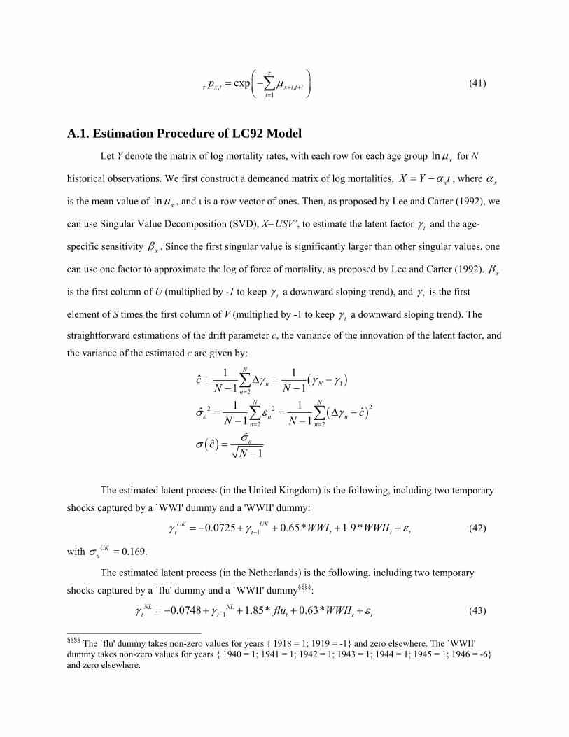
A.1. Estimation Procedure of LC92 Model

Let Y denote the matrix of log mortality rates, with each row for each age group ln xμ for N

historical observations. We first construct a demeaned matrix of log mortalities, xX Y α ι= − , where xα

is the mean value of ln xμ , and ι is a row vector of ones. Then, as proposed by Lee and Carter (1992), we

can use Singular Value Decomposition (SVD), X=USV’, to estimate the latent factor tγ and the age-

specific sensitivity xβ . Since the first singular value is significantly larger than other singular values, one

can use one factor to approximate the log of force of mortality, as proposed by Lee and Carter (1992). xβ

is the first column of U (multiplied by -1 to keep tγ a downward sloping trend), and tγ is the first

element of S times the first column of V (multiplied by -1 to keep tγ a downward sloping trend). The

straightforward estimations of the drift parameter c, the variance of the innovation of the latent factor, and

the variance of the estimated c are given by:

( )

( )

( )

12

22 2

2 2

1 1ˆ1 11 1ˆ ˆ

1 1ˆˆ

1

N

n Nn

N N

n nn n

cN N

cN N

cN

ε

ε

γ γ γ

σ ε γ

σσ

=

= =

= Δ = −− −

= = Δ −− −

=−

∑

∑ ∑

The estimated latent process (in the United Kingdom) is the following, including two temporary

shocks captured by a `WWI' dummy and a 'WWII' dummy:

10.0725 0.65* 1.9*UK UKt t t t tWWI WWIIγ γ ε−= − + + + + (42)

with UKεσ = 0.169.

The estimated latent process (in the Netherlands) is the following, including two temporary

shocks captured by a `flu' dummy and a `WWII' dummy§§§§:

10.0748 1.85* 0.63*NL NLt t t t tflu WWIIγ γ ε−= − + + + + (43)

§§§§ The `flu' dummy takes non-zero values for years { 1918 = 1; 1919 = -1} and zero elsewhere. The `WWII' dummy takes non-zero values for years { 1940 = 1; 1941 = 1; 1942 = 1; 1943 = 1; 1944 = 1; 1945 = 1; 1946 = -6} and zero elsewhere.

with NLεσ = 0.2176. As pointed out in Lee-Carter (1992), the dummy variables only reduced the standard

errors of the mortality forecast, but not the trend itself.

A.2. Simulation The simulation steps:

1. Simulate the latent factor for T periods according to i 1ˆ i icγ γ ε−= + + , for i = 1,...,T, where

( )2~ 0,i N εε σ , and 0γ is obtained from the estimation of year 2003.

2. Compute the force of mortality according to ( ),ln x i t i x i x i t iμ α β γ+ + + + += + for i =1,...,T.

3. Compute the survival probability of the x-year-old cohort according to

( ) ⎟⎠

⎞⎜⎝

⎛−= ∑

=++

τ

τ μ1

,expi

itixx tp , for τ= 1,...,T.

4. Compute the survival index xtt pNS = , where N is the initial size of the cohort.

5. Repeat 1-4 steps for M times. As a by-product, calculate the mean, variance, and confidence

interval of the forecasted survival probabilities and the survival index.

Appendix B. Derivation of the Results in Section 4 First introduce some notations. For any given value of b∈[0,1], we have the marginal utility

( ) ( )xxu α−= exp' , and the inverse function of the marginal utility as ( )zI v ln1α

−= . The inverse

function of the utility function is denoted as ( )zIu αα

−−= ln1.

Problem 1 (continued) without longevity risk

Set up the Lagrange

( ) ( ) ⎟⎠⎞⎜

⎝⎛

⎥⎦⎤

⎢⎣⎡ +−+⎥⎦

⎤⎢⎣⎡ += ∫∫ −−

TT

T

ttTTT

tt WMdtDMEWWuedtDueEL

000φδδ (44)

( )

( ) TTT

T

ttt

t

MWueWL

MDueDL

φ

φ

δ

δ

=⇒=∂∂

=⇒=∂∂

−

−

'0

'0

The optimal strategies are

( ) ( )

( ) ( )TT

TT

vT

tt

tt

vt

MeMeIW

MeMeID

φα

φ

φα

φ

δδ

δδ

ln1

ln1

*

*

−==

−==

Plug into the budget constraint and the indirect utility function, we have

( ) ( )⎥⎦⎤

⎢⎣⎡ +−=⎥⎦

⎤⎢⎣⎡ += ∫∫ T

TT

T

tt

tTT

T

tt MeMdtMeMEWMdtDMEW φφα

δδ lnln10

*

0

*0 (45)

( ) ( ) ⎥⎦⎤

⎢⎣⎡ +−=⎥⎦

⎤⎢⎣⎡ += ∫∫ −−

T

T

tTTT

tt MdtMEWuedtDueEV

0

*

0

*0

1 φα

δδ (46)

Problem 2 (continued) with longevity risk

Set up the Lagrange

[ ]( ) ( ) ⎟⎠⎞⎜

⎝⎛

⎥⎦⎤

⎢⎣⎡ +−++⎥⎦

⎤⎢⎣⎡ +−+= ∫∫ −− πππδπδ πφ TT

T

ttTTT

tttt WMdtDMEWWuedtSSEDueEL

000

Since longevity risk, [ ] tt SSE − , cannot be hedged in the modelled financial market, the optimal

strategy, πtD , is independent from [ ] tt SSE − . Under the assumed preference (10), the above Lagrange

can be rewritten as

( ) [ ]( )( )[ ] ( )

( ) ( ) ⎟⎠⎞⎜

⎝⎛

⎥⎦⎤

⎢⎣⎡ +−++⎥⎦

⎤⎢⎣⎡ +=

⎟⎠⎞⎜

⎝⎛

⎥⎦⎤

⎢⎣⎡ +−++

⎥⎦⎤

⎢⎣⎡ +−−−−=

∫∫

∫

∫

−−

−−

ππππδπδ

πππ

πδπδ

πφ

πφ

ααα

TT

T

ttTTT

ttt

TT

T

tt

TTT

tttt

WMdtDMEWWuedtGDueE

WMdtDMEW

WuedtSSEEDeEL

000

00

0expexp1

Where [ ]( )( )[ ]ttt SSEEG −−≡ αexp and α is the shorthand notation for ( ) bWW −= 00 αα . tG can be

seen as a function of the certainty equivalent of [ ] tt SSE − .

The optimal dividend strategy can be found by

( )

( ) TTT

T

tttt

t

MWueW

L

MGDueDL

ππδπ

ππδπ

φ

φ

=⇒=∂∂

=⇒=∂∂

−

−

'0

'0

The optimal strategies are

( ) ( )ttt

tt

vt GMeMeID lnln1* −−== πδπδπ φα

φ (47)

( ) ( )TT

TT

vT MeMeIW πδπδπ φα

φ ln1* −== (48)

Plug into the budget constraint and the indirect utility function

( ) ( ) ⎥⎦

⎤⎢⎣⎡+⎥⎦

⎤⎢⎣⎡ +−=

⎥⎦⎤

⎢⎣⎡ +=+

∫∫

∫T

ttTT

T

T

tt

t

TT

T

tt

dtGMEMeMdtMeME

WMdtDMEW

00

*

0

*0

ln1lnln1α

φφα

π

πδπδ

ππ

(49)

( ) ( ) ⎥⎦⎤

⎢⎣⎡ +−=⎥

⎦

⎤⎢⎣

⎡+⎟

⎠⎞

⎜⎝⎛ −−= ∫∫ −−

T

T

tTTT

ttt MdtMEWuedtGDeEV

0

*

0

*0

1exp1 ππδπδπ φα

αα

(50)

Equalizing the two indirect utilities (46) and (50), π00 VV = , we find πφφ = . Comparing

the two budget constraints (45) and (49), with πφφ = , we have

( ) ( )⎥⎦⎤

⎢⎣⎡ +−= ∫ T

TT

T

tt

t MeMdtMeMEW φφα

δδ lnln100 (51)

( ) ( ) ⎥⎦⎤

⎢⎣⎡+⎥⎦

⎤⎢⎣⎡ +−=+ ∫∫

T

ttTT

T

T

tt

t dtGMEMeMdtMeMEW000 ln1lnln1

αφφ

απ δδ (52)

The difference between the two budget constraints gives the expression for longevity risk loading of the survival bond as

[ ]

∫

∫∫−=

=⎥⎦⎤

⎢⎣⎡=

T

trt

T

tt

T

tt

dtGe

dtGMEdtGME

0

00

ln1

ln1ln1

α

ααπ

(53)

where [ ]( )( )[ ]ttt SSEEG −−= αexp .