longitudinal waves - harvard university2 chapter 5. longitudinal waves for a transverse wave, ˆ is...

Chapter 5

Longitudinal wavesDavid Morin, [email protected]

In Chapter 4 we discussed transverse waves, in particular transverse waves on a string. We’llnow move on to longitudinal waves. Each point in the medium (whatever it consists of)still oscillates back and forth around its equilibrium position, but now in the longitudinalinstead of the transverse direction. Longitudinal waves are a bit harder to visualize thantransverse waves, partly because everything is taking place along only one dimension, andpartly because of the way the forces arise, as we’ll see. Most of this chapter will be spenton sound waves, which are the prime example of longitudinal waves.

The outline of this chapter is as follows. As a warm up, in Section 5.1 we take anotherlook at the longitudinal spring/mass system we originally studied in Section 2.4, where weconsidered at the continuum limit (the N → ∞ limit). In Section 5.2 we study actualsound waves. We derive the wave equation (which takes the same form as all the other waveequations we’ve seen so far), and then look at the properties of the waves. In Section 5.3we apply our knowledge of sound waves to musical instruments.

5.1 Springs and masses revisited

Recall that the wave equation for the continuous spring/mass system was given in Eq. (2.80)as

∂2ψ(x, t)

∂t2=

E

µ

∂2ψ(x, t)

∂x2, (1)

where ψ is the longitudinal position relative to equilibrium, µ is the mass density, and E isthe elastic modulus. This wave equation is very similar to the one for transverse waves ona string, which was given in Eq. (4.4) as

∂2ψ(x, t)

∂t2=

T

µ

∂2ψ(x, t)

∂x2, (2)

where ψ is the transverse position relative to equilibrium, µ is the mass density, and T isthe tension.

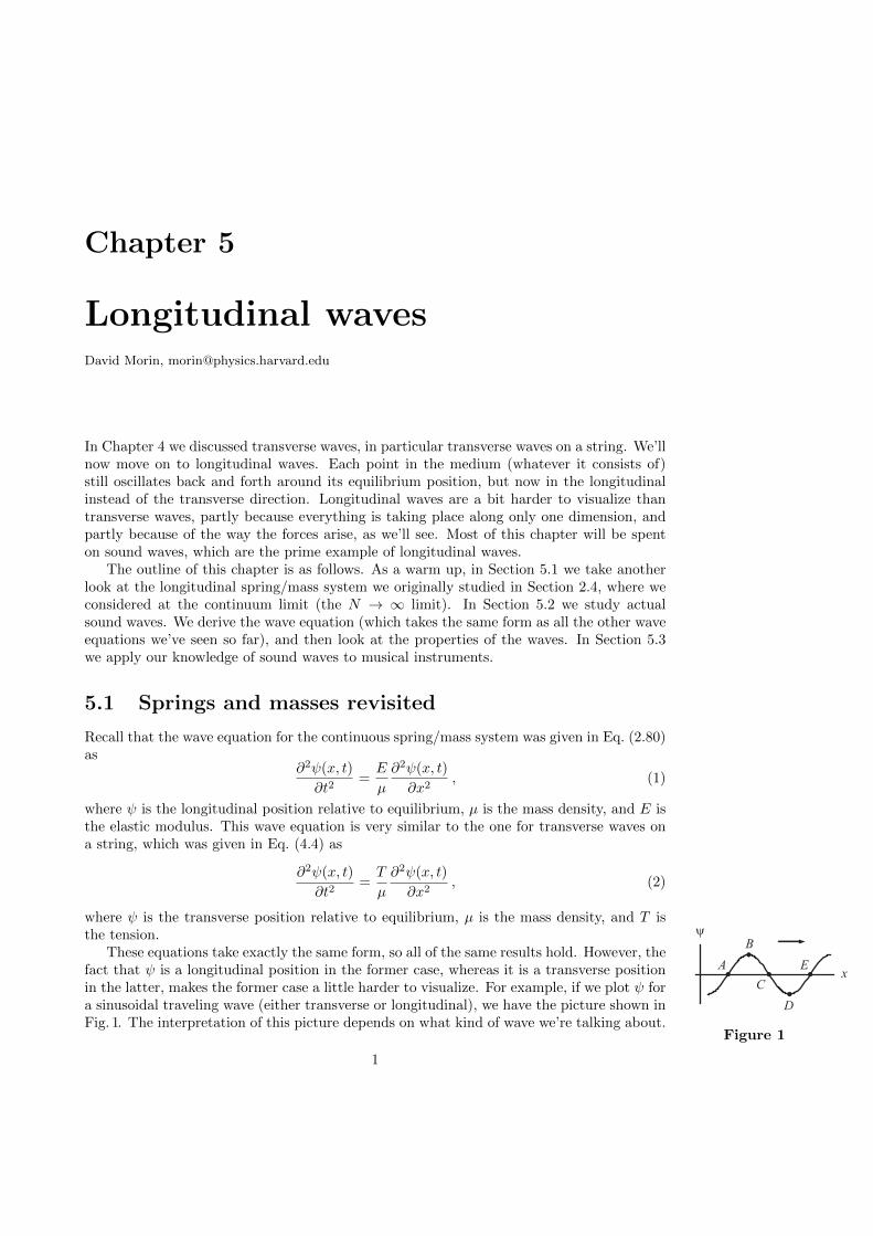
These equations take exactly the same form, so all of the same results hold. However, thefact that ψ is a longitudinal position in the former case, whereas it is a transverse positionin the latter, makes the former case a little harder to visualize. For example, if we plot ψ fora sinusoidal traveling wave (either transverse or longitudinal), we have the picture shown inFig. 1. The interpretation of this picture depends on what kind of wave we’re talking about.

x

ψ

A

B

C

D

E

Figure 1

1

2 CHAPTER 5. LONGITUDINAL WAVES

For a transverse wave, ψ is the transverse displacement, so Fig. 1 is what the stringactually looks like from the side. The wave is therefore very easy to visualize – you justneed to look at the figure. It’s also fairly easy to see what the various points in Fig. 1 aredoing as the wave travels to the right. (Imagine that these dots are painted on the string.)Points B and D are instantaneously at rest, points A and E are moving downward, andpoint C is moving upward. To verify these facts, just draw the wave at a slightly later time.The result is shown in Fig. 2, with the new positions of the dots being represented by gray

x

ψ

wave at a

later time

A

B

C

D

E

Figure 2dots. Remember that the points keep their same longitudinal position and simply move upor down (or not at all). They don’t travel longitudinally along with the wave.

However, for a longitudinal wave, ψ is the longitudinal displacement, so although Fig. 1is a perfectly valid plot of ψ, it does not indicate what the wave actually looks like. Thereis no transverse motion, so the system simply lies along a straight line. What changes isthe density along the line. You could therefore draw the wave by shading it as in Fig. 3,

x

A B C D E

Figure 3

but this is a bit harder to draw than Fig. 1. For a longitudinal wave, the statements in thepreceding paragraph about the motion of the various points in Fig. 1 are still true, providedthat “downward” is replaced with “leftward,” and “upward” is replaced with “rightward.But what do things actually look like along the 1-D line? In particular, how does Fig. 3follow from Fig. 1?

At points B and D in Fig. 3, the density of the masses equals the equilibrium density,because nearby points all have essentially the same displacement (see Fig. 1). But at pointsA and E, the density is a minimum, because points to the left of them have a negativedisplacement, while points to the right have a positive displacement (again see Fig. 1). Theopposite is true for point C, so the density is maximum there. Various properties of thewave are indicated in Fig. 4. You should stare at this figure for a while and verify all of thestated properties. We’ll talk more about the relation among the various quantities when wediscuss Fig. 8 later on when we get to sound waves.

max +ψ, v = 0, max -a, avg ρ

max -ψ, v = 0, max +a, avg ρ

ψ = 0, max +v, a = 0, max +ρ

ψ = 0, max -v, a = 0, max -ρ

x

ψ

positive position

positive velocity

positive acceleration

rightward traveling

Figure 4

In the Fig. 4, the relation between ψ, v, and a is the same as always, namely, a is 90◦

ahead of v, and v is 90◦ ahead of ψ. But you should think about how these relate to thedensity ρ. For example, from the preceding paragraph, the (excess) ρ is proportional to thenegative of the slope (see Problem [to be added] for a rigorous derivation of this fact). Butwe already know that v is proportional to the negative of the slope; see Eq. (4.44). Therefore,the (excess) ρ is proportional to v. For a leftward traveling wave, the same statement about

5.2. SOUND WAVES 3

ρ is still true, but now v is proportional to the slope (with no negative sign). So the (excess)ρ is proportional to −v.

We can double check that this result makes sense with the following reasoning. Sincethe (excess) ρ is proportional to v, we can take the derivative of this statement to say that∂ρ/∂x ∝ ∂v/∂x (the word “excess” is now not needed). But since a traveling wave takesthe form of ψ(x, t) = f(x − ct), the velocity v = ∂ψ/∂t also takes the functional form ofg(x− ct). Therefore, we have ∂v/∂x = −(1/c)∂v/∂t. The righthand side of this is just theacceleration a, so the ∂ρ/∂x ∝ ∂v/∂x statement becomes

∂ρ

∂x∝ −a =⇒ a ∝ −∂ρ

∂x. (3)

Does this make sense? It says, for example, that if the density is an increasing function ofx at a given point, then the acceleration is negative there. This is indeed correct, becausea larger density means that the springs are more compressed (or less stretched), which inturn means that they exert a larger repulsive force (or a smaller attractive force). So if thedensity is an increasing function of x (that is, if ∂ρ/∂x > 0), then the springs to the right of agiven region are pushing leftward more than the springs to the left of the region are pushingrightward. There is therefore a net negative force, which means that the acceleration a isnegative, in agreement with Eq. (3).

5.2 Sound waves

5.2.1 Notation

Sound is a longitudinal wave, in both position and pressure/density, as we’ll see. Sound canexist in solids, liquids, and gasses, but in this chapter we’ll generally work with sound wavesin air. In air, molecules push and (effectively, relative to equilibrium) pull on each other, sowe have a sort of spring/mass system like the one we discussed above.

The main goal in this section is to derive the wave equation for sound waves in air. We’llfind that we obtain exactly the same type of wave equation that we had in Eq. (1) for thespring/mass system. The elastic modulus E appears there, so part of our task below willbe to find the analogous quantity for sound waves. We’ll consider only one-dimensionalwaves here. That is, the waves depend only on x. Waves like this that are uniform in thetransverse y and z directions are called “plane waves.”

To emphasize the 1-D nature of the wave, let’s consider a tube of air inside a cylindricalcontainer, with cross-sectional area A. Fig. 5 shows a given section of air at equilibrium,and then also at a later time. Let the ends of this section be located at x and x + ∆x atequilibrium, and then at x + ψ(x) and x +∆x + ψ(x +∆x) at a later time, as shown. Sothe function ψ measures the displacement from equilibrium.

If we define ∆ψ by ψ(x + ∆x) ≡ ψ(x) + ∆ψ, then ∆ψ is how much more the rightboundary of the region moves compared with the left boundary. The molecules of air are inthermal motion, of course, so it’s not as if the molecules that form the boundary at positionx in the first picture correspond to the molecules that form the boundary at position x+ψ(x)in the second picture. But we’ll ignore this fact and just pretend that it’s the same molecules,for ease of discussion. It doesn’t actually matter. Note that ∆ψ ≈ (∂ψ/∂x)∆x for small∆x, by definition of the derivative. In actual sound waves in air, ∆ψ is much less than ∆x.In other words, ∂ψ/∂x is very small.


(equilibrium)

(later)

x x+∆x

x+∆x+ψ(x+∆x)

x+∆x+ψ(x)+∆ψ

∆x+∆ψ

x+ψ(x)

Figure 5

A note on terminology: We’re taking x to be the position of a given molecule at equilib-rium. So even after the molecule has moved to the position x + ψ(x), it is still associatedwith the same value of x. So x is analogous to the index n we used in Section 2.3 and thebeginning of Section 2.4. The movement of the particle didn’t affect its label n there, andit doesn’t affect its label x here.

In obtaining the wave equation, we’ll need to get a handle on the pressure at the two endsof the given section of air, and then we’ll figure out how these pressures cause the sectionto move. Let the pressure in the tube at equilibrium be p0. At sea level, the atmosphericpressure happens to be about 14.7 lbs. per square inch. The first picture in Fig. 6 showsthe pressures at the two ends at equilibrium; it is simply p0 at both ends (and everywhereelse).

(equilibrium)

(later)

x

p0 p0

p(x)=p0+ψp(x) p(x+∆x) = p0+ψp(x+∆x)

p0+ψp(x)+∆ψp

x+∆x

Figure 6

What about at a later time? Let ψp(x) be the excess pressure (above p0) as a functionof x. (Remember that x labels the equilibrium position of the molecules, not the presentposition.) The total pressure at the left boundary of the section is then p0+ψp(x). However,this total pressure won’t be too important; the change, ψp(x), is what we’ll be concernedwith. At the right boundary, the total pressure is, by definition, p0 + ψp(x + ∆x). If wedefine ∆ψp by ψp(x + ∆x) ≡ ψp(x) + ∆ψp, then ∆ψp is how much the pressure at theright boundary exceeds the pressure at the left boundary. Note that ∆ψp ≈ (∂ψp/∂x)∆xfor small ∆x. In practice, ψp is much smaller than p0. And ∆ψp is infinitesimally small,assuming that we have picked ∆x to be infinitesimally small. The pressures at a later timeare summarized in the second picture in Fig. 6.

5.2. SOUND WAVES 5

5.2.2 The wave equation

Having introduced the necessary notation, we can now derive the wave equation for soundwaves. The derivation consists of four main steps, so let’s go through them systematically.Our strategy will be to find the net force on a given volume of air, and then write down theF = ma equation for that volume.

1. How the volume changes: First, we need to determine how the volume of a gaschanges when the pressure is changed. Qualitatively, if we increase the pressure ona given volume, the volume decreases. By how much? The decrease should certainlybe proportional to the volume, because if we put two copies of a given volume nextto each other, we will obtain twice the decrease. And the decrease should also beproportional to the pressure increase, provided that the increase is small. This is areasonable claim, but not terribly obvious. We’ll derive it in step 2 below. Assumingthat it is true, we can write (recalling that ψp is defined to be the increase in pressurerelative to equilibrium) the change in volume from equilibrium as ∆V ∝ −V ψp. Thiscorrectly incorporates the two proportionality facts above. The minus sign is due tothe fact that an increase in pressure causes a decrease in volume. This equation isvalid as long as ∆V is small compared with V , as we’ll see below.

Let’s define κ to be the constant of proportionality in ∆V ∝ −V ψp. κ is known as thecompressibility. The larger κ is, the more the volume is compressed (or expanded), fora given increase (or decrease) in pressure, ψp. In terms of κ, we have

∆V = −κV ψp. (4)

But from the first picture in Fig. 5, we see that the volume of gas is V = A∆x, whereA is the cross-sectional area. And the change in the volume between the two picturesshown is ∆V = A∆ψ.1 Eq. (4) therefore becomes

∆V

V= −κψp =⇒ A∆ψ

A∆x= −κψp =⇒ ∂ψ

∂x= −κψp (5)

where we have taken the infinitesimal limit and changed the ∆’s to differentials (par-tial ones, since ψ is a function of t also). The quantity ∂ψ/∂x indicates how thedisplacement from equilibrium grows as a function of x. Equivalently, ∂ψ/∂x is the“stretching fraction.” If the displacement ψ grows by, say, 1 mm over the course ofa distance of 10 cm, then the length (and hence the volume) of the region has in-creased by 1/100, and this equals ∂ψ/∂x. Eq. (5) says that the stretching fraction isproportional to the change in pressure, which is quite reasonable.

2. Calculating the compressibility, κ: We’ll now be rigorous about the abovestatement that the decrease in volume should be proportional to the pressure increase,provided that the increase is small. In the course of doing this, we’ll find the value ofκ.

Let’s first give a derivation that isn’t quite correct. From the ideal gas law (which we’llaccept here; we have to start somewhere), we have pV = nRT . If the temperatureT is constant, then any changes in p and V must satisfy (p + dp)(V + dV ) = nRT .Subtracting the original pV = nRT equation from this one, and ignoring the second-order dp dV term (this is where the assumption of small changes comes in), we obtain

1We can alternatively say that the volume is V = A(∆x + ∆ψ), by looking at the second picture. Butwe are assuming ∆ψ ¿ ∆x, so to leading order we can ignore the A∆ψ term in the volume. However, wecan’t ignore it in the change in volume, because it’s the entire change.


p dV + dp V = 0 =⇒ dV = −(1/p)V dp. But dp is what we’ve been calling ψp above,so if we compare this result with Eq. (4), we see that the compressibility κ equals 1/p.Note that what we did here was basically take the differential of the pV = C equation(where C is a constant) to obtain p dV + dp V = 0.

However, this κ = 1/p result isn’t correct, because it is based on the assumption that Tis constant in the relation pV = nRT . But T isn’t constant in a sound wave (in eitherspace or time). The compressions are actually adiabatic, meaning that heat can’t flowquickly enough to redistribute itself and even things out. Basically, the time scaleof the heat flow is large compared with the time scale of the wave oscillations. So aregion that heats up due to high pressure stays hot, until the pressure decreases. Thecorrect relation (which we’ll just accept here) for adiabatic processes turns out to bepV γ = C, where γ happens to be about 7/5 for air (γ is 7/5 for a diatomic gas, andair is 99% N2 and O2). Taking the differential of our new pV γ = C equation gives

p · γV γ−1 dV + dp V γ = 0 =⇒ dV = −(

1

γp

)V dp. (6)

Therefore, the correct value of the compressibility κ is

κ =1

γp0≈ 5

7p0. (7)

The above incorrect result wasn’t so bad; it was off by only a factor of 7/5.

3. Calculating the difference in pressure, ∆ψp: Eq. (5) involves the quantityψp. However, what we’re actually concerned with is not ψp but the change in ψp fromone end of the volume to the other, because in writing down the F = ma equation forthe volume, we’re concerned with the net force on it, and this involves the differencein the pressures at the ends. So let’s see how ψp changes with x. Differentiating Eq.(5) with respect to x gives

∂ψp

∂x= − 1

κ

∂2ψ

∂x2=⇒ ∆ψp = − 1

κ

∂2ψ

∂x2∆x, (8)

where we have multiplied both sides by ∂x and switched back to the ∆ notation.Or equivalently, we have multiplied both sides by ∆x, and then used the relation∆ψp = (∂ψp/∂x)∆x. Note that the second derivative ∂2ψ/∂x2 appears here. FromEq. (5), a constant value of ∂ψ/∂x corresponds to a constant excess pressure ψp(x);the tube of air just stretches uniformly if the pressure is the same everywhere. So toobtain a varying value of ψp, we need a varying value of ∂ψ/∂x. That is, we need anonzero value of ∂2ψ/∂x2.

4. The F = ma equation: We can now write down the F = ma equation for a givenvolume of air. The net rightward force on the tube of air in the second picture in Fig.6 is the cross-sectional area times the difference in the pressure at the ends. So wehave, recalling the definition of ∆ψp,

Fnet = A(p(x)− p(x+∆x)

)= A(−∆ψp). (9)

Using the expression for ∆ψp we found in Eq. (8), the Fnet = ma equation on a giventube of air is (with ρ being the mass density)

−A∆ψp = (ρV )∂2ψ

∂t2

=⇒ −A

(− 1

κ

∂2ψ

∂x2∆x

)= ρ(A∆x)

∂2ψ

∂t2. (10)

5.2. SOUND WAVES 7

Canceling the common factor of A∆x and using κ = 1/γp0 yields

∂2ψ

∂t2=

γp0ρ

· ∂2ψ

∂x2(wave equation) (11)

This is the desired wave equation for sound waves in air. We see that γp0/ρ is thecoefficient that replaces the E/µ coefficient for the longitudinal spring/mass system,or the T/µ coefficient for the transverse string.

The solutions to the wave equation are the usual exponentials,

ψ(x, t) = Aei(±kx±ωt), (12)

where ω and k satisfy ω/k =√γp0/ρ. And since ω/k is the speed c of the wave, we have

c =√γp0/ρ. As always, the speed is simply the square root of the factor on the righthand

side. As a double check on the units, we have

γp0ρ

=(unitless) · (force/area)

mass/volume=

(kgm/s2)/m2

kg/m3=

m2

s2, (13)

which has the correct units of velocity squared. What is the numerical value of the speedof sound waves? For air at sea level, the pressure is p0 ≈ 105 kg/ms2 and the density isρ ≈ 1.3 kg/m3. So we have

c =

√γp0ρ

≈√

(7/5)(105 kg/ms2)

1.3 kg/m3≈ 330m/s. (14)

This decreases with ρ, which makes sense because the larger the density, the more inertiathe air has, so the harder it is to accelerate it. The speed increases with p0. This followsfrom the fact that if p0 is large, then the compressibility κ is small (meaning the gas is noteasily compressed). So for a given value of ∂2ψ/∂x2, the force on the left side of Eq. (10) islarge, which implies large accelerations.

The two partial derivatives in Eq. (11) come about in the usual way. The second timederivative comes from the “a” in F = ma, and the second space derivative comes from thefact that it is the difference in the first derivatives that gives the net force. Eq. (5) tells usthat the first space derivative of the displacement gives a measure of the force at a givenlocation (just as with the spring/mass system, the first space derivative told us how muchthe springs were stretched, which in turn gave the force). The difference in the force at thetwo ends is therefore proportional to the second space derivative (again as it was with thespring/mass system).

As with the other wave equations we have encountered thus far in this book, the speedof sound waves is independent of ω and k. (This won’t be the case for the dispersion-fulwaves we discuss in the following chapter.) So all frequencies travel at the same speed. Thisis fortunate, because if it weren’t true, then a music concert would sound like a completemess!

5.2.3 Pressure waves

Eq. (11) gives the wave equation for the displacement, ψ, from equilibrium for a moleculewhose equilibrium position is x. However, it is rather difficult to follow the motion of a singlemolecule, so it would be nice to obtain the wave equation for the excess pressure ψp, becausethe pressure is much easier to measure. (It is a macroscopic property of the average of a


large number of molecules, as opposed to the microscopic position of a particular molecule.)In view of the relation between ψp and ψ in Eq. (5), we can generate the wave equationfor ψp by taking the ∂/∂x derivative of the wave equation in Eq. (11). Using the fact thatpartial derivatives commute, we obtain

∂

∂x

(∂2ψ

∂t2

)=

γp0ρ

· ∂

∂x

(∂2ψ

∂x2

)=⇒ ∂2

∂t2

(∂ψ

∂x

)=

γp0ρ

· ∂2

∂x2

(∂ψ

∂x

). (15)

But from Eq. (5) we know that ∂ψ/∂x ∝ ψp, so we obtain

∂2ψp

∂t2=

γp0ρ

· ∂2ψp

∂x2(wave equation for pressure) (16)

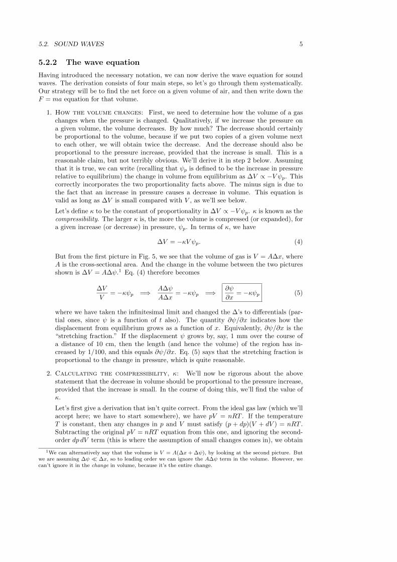
This is the same wave equation as the one for the displacement ψ in Eq. (11). So everythingthat is true about ψ is also true about ψp. The only difference is that since ψp ∝ −∂ψ/∂x(the minus sign is important here), the phase of ψp is 90◦ behind the phase of ψ. This isshown in Fig. 7. The pressure (and hence also the density) reaches its maximum value a

x

ψ,ψp ψψp

Figure 7quarter cycle after the displacement does. This is consistent with the values of ψ and ρgiven in Fig. 4.

5.2.4 Impedance

What is the impedance of air? In other words, what is the force per velocity that a givenregion applies to an adjacent region, as a wave propagates? Remember that impedance is aproperty of the medium and not the wave, even though it is generally easiest to calculate itby considering the properties of a traveling wave. (However, when we discuss dispersion-fulsystems in the next chapter, we will find that the impedance depends on the frequency ofthe wave.)

The velocity of a “sheet” of molecules whose equilibrium position is x is simply v(x) =∂ψ(x)/∂t. To find the force, consider a cross-sectional area A. We can use Eq. (5) to writethe (excess) force that the sheet exerts on the region to its right as

F = Aψp = A

(− 1

κ

∂ψ

∂x

). (17)

And since we are working with a traveling wave (no need for it to be sinusoidal), we havethe usual relationship between ∂ψ/∂x and ∂ψ/∂t, namely ∂ψ/∂x = ∓(1/c)(∂ψ/∂t) (theminus sign is associated with a rightward traveling wave). So Eq. (17) becomes

F = A

(− 1

κ

)(∓1

c

∂ψ

∂t

)= ± A

κc· ∂ψ∂t

. (18)

The force that the sheet feels from the region on its right is the negative of this, but the signisn’t important when calculating the impedance Z, because Z is defined to be the magnitudeof F/v. Using v = ∂ψ/∂t, Eq. (18) gives the impedance as

Z ≡ F

v=

A

κc. (19)

The impedance per unit area is the more natural thing to talk about, because Z/A isindependent of the specific cross section chosen. The force F can be made arbitrarily largeby making the area A arbitrarily large, so Z = F/v isn’t too meaningful. When peopletalk about the impedance of air, they usually mean “impedance per area,” that is, force

5.2. SOUND WAVES 9

per velocity per area. However, we’ll stick with the Z = F/v definition of impedance,in which case Eq. (19) tells us that the impedance per unit area is Z/A = 1/κc. Butc = 1/

√κρ =⇒ κ = 1/ρc2 (this follows from writing the coefficient in Eq. (11) in terms of

κ). So we have Z/A = ρc. Using c =√γp0/ρ from Eq. (14), we can write this alternatively

as

Z

A= ρc =

√γρp0 (20)

5.2.5 Energy, Power

Energy

What is the energy density of a (longitudinal) sound wave? The kinetic energy density (perunit volume) is simply (1/2)ρ(∂ψ/∂t)2, because the speed of the molecules is ∂ψ/∂t. Ifwe want to consider instead the kinetic energy density per unit length along a tube withcross-sectional area A, then this is (1/2)(Aρ)(∂ψ/∂t)2, where Aρ ≡ µ is the mass densityper unit length. We are assuming here that ρ and µ are independent of position. This isessentially true for actual sound waves, because ∂ψ/∂x is small, so the fractional change inthe density from its equilibrium value is small.

What about the potential energy density? The task of Problem [to be added] is toshow that the potential energy density (or rather, the excess over the equilibrium value) perunit length is (1/2)Aγp0(∂ψ/∂x)

2. The total energy density per unit length (kinetic pluspotential) is therefore

E(x, t) =1

2Aρ

(∂ψ

∂t

)2

+1

2Aγp0

(∂ψ

∂x

)2

=1

2Aρ

[(∂ψ

∂t

)2

+γp0ρ

(∂ψ

∂x

)2]

=1

2Aρ

[(∂ψ

∂t

)2

+ c2(∂ψ

∂x

)2]. (21)

This is the same as the result we found in Eq. (4.49) for transverse waves, since Aρ is themass per unit length, µ. As with Eq. (4.49), the present expression for E(x, t) is valid foran arbitrary wave. But if we consider the special case of a single traveling wave, then wehave the usual relation, ∂ψ/∂t = ±c ∂ψ/∂x. So the two terms in the expression for E(x, t)are equal at a given point and at a given time. We can therefore write the energy densityper unit length as

E(x, t) = Aρ

(∂ψ

∂t

)2

(for traveling waves) (22)

The energy density per unit volume is then E/A = ρ(∂ψ/∂t)2.

Power

Consider a cross-sectional “sheet” of molecules. At what rate does the air on the left of thesheet do work on the sheet? (This is the same type of question that we asked in Section4.4 for a transverse wave: At what rate does the string to the left of a dot do work on thedot?) In a small amount of the time, the work done by the air is dW = F dψ = (pA) dψ.


The power on the sheet whose equilibrium position is x is therefore

P =∂W

∂t= (p0 + ψp)A

∂ψ

∂t. (23)

The Ap0(∂ψ/∂t) part of this averages out to zero over time, so we’ll ignore it. TheAψp(∂ψ/∂t) term, however, always has the same sign, for the following reason. From Eq.(5), we have ψp = −(1/κ)(∂ψ/∂x). But as usual, ∂ψ/∂x = ∓(1/c)(∂ψ/∂t) (the minus signis associated with a rightward traveling wave). So the power is

P = Aψp∂ψ

∂t= A

(± 1

κc· ∂ψ∂t

)∂ψ

∂t= ± A

κc

(∂ψ

∂t

)2

. (24)

Using c = 1/√κρ =⇒ κ = 1/ρc2, we have

P = ±Aρc

(∂ψ

∂t

)2

(25)

Since Z = Aρc from Eq. (20), we can also write the power as

P = ±Z

(∂ψ

∂t

)2

, (26)

which takes exactly the same form as the result in Eq. (4.53) for transverse waves.If we compare Eqs. (22) and (25), we see that P = ±cE . This makes sense, because

as with transverse waves, the power must equal the product of the wave velocity and theenergy density, because the E curve moves right along with the wave.

If we want to write P in terms of the pressure ψp, we can do this in the following way.Using Eq. (5), Eq. (25) becomes

P = ±Aρc

(∓c

∂ψ

∂x

)2

= ±Aρc3(−κψp)2 = ±Aρc3

(1

ρc2

)2

ψ2p = ±A

ρcψ2p (27)

We see that when written in terms of ψp, the power decreases with ρ and c. But whenwritten in terms of ψ (or rather ∂ψ/∂t) in Eq. (25), it grows with ρ and c. The latteris fairly clear. For example, a larger ρ means that more matter is moving, so the energydensity is larger. But the dependence on ψp isn’t as obvious. It arises from the fact thatthere are factors of ρ and c hidden in ψp. So, for example, if ρ is increased (for a givenfunction ψ), then ψ2

p grows faster than ρ, so the righthand side of Eq. (27) still increaseswith ρ. However, if ρ is increased for a given function ψp, then the power decreases, becausethe displacement ψ has to decrease to keep ψp the same, and this effect wins out over theincrease in ρ, thereby decreasing P .

5.2.6 Qualitative description

Let’s take a look at what a given molecule in the air is doing at a few different times, as arightward-traveling wave passes by. A number of snapshots with phase differences of π/4are shown in Fig. 8. The darker regions indicate a higher pressure (and density), and thelighter regions indicate a lower pressure (and density). The vertical line, which representsthe equilibrium position of the molecule, is drawn for clarity.

The three plots at the top of the figure give the values of the various parameters at t = 0,as functions of x. So these plots correspond to the first of the shaded snapshots. The plots

5.2. SOUND WAVES 11

for the eight other snapshots are obtained by simply shifting the three plots to the right, bythe same amount as the snapshots shift. The three plots at the left of the figure give thevalues of the various parameters at x = 0, as functions of t. So these plots correspond tothe molecule in question (the little circle). The leftmost plot (the one for ψ(0, t)) is simplya copy of the circles as they appear in the snapshots.2

Let’s discuss what’s happening in each of the snapshots. In doing this, a helpful thing toremember is that for a rightward-traveling wave, the density (and hence pressure) is alwaysin phase with the velocity (as we discussed in Section 5.1). And both the pressure and thevelocity are 90◦ ahead of the position, as functions of time. (For a leftward-traveling wave,the pressure is out of phase with the velocity, which is, as always, 90◦ ahead of the position.)Again, the displacements are exaggerated in the figures. In reality, the displacements aremuch smaller than the wavelength. The commentary on the snapshots is as follows.

ψ(0,t) v(0,t)

ψp(0,t)

a(0,t)

t

1.

2.

3.

4.

5.

6.

7.

8.

9.

ψ(x,0)

v(x,0), ψp(x,0)

a(x,0)

(t=0)

(x=0)xplots for t=0,as functions of x

plots for x=0,as functions of t

0

0

(Exaggerated displacements

of the molecule)

Figure 8

2The ψ values are exaggerated for emphasis. In reality, they are much smaller than the wavelength ofthe wave. But if we drew them to scale, all of the circles would essentially lie on the x = 0 line, and wewouldn’t be able to tell that they were actually moving.


1. In the first snapshot, the molecule is located at its equilibrium position and is movingto the right with maximum speed.3 The pressure (and density) is also maximum. Thepressure is the same on both sides of the molecule, so there is zero net force, consistentwith the fact that it has maximum speed and hence zero acceleration.

2. The molecule is still moving to the right, but it is decelerating (a < 0) because thereis higher pressure (which goes hand-in-hand with higher density) on its right than onits left.

3. It has now reached its maximum value of ψ and is instantaneously at rest. It has themaximum negative acceleration, because the pressure gradient is largest here; the pres-sure is changing most rapidly (as a function of x) halfway between the maximum andminimum pressures. The difference between the forces on either side of the moleculeis therefore largest here, so the molecule experiences the largest acceleration.

4. It has now started moving leftward and is picking up speed due to the higher pressureon the right.

5. It passes through equilibrium again, but now with the maximum negative velocity.This ends the period of negative acceleration. Up to this time, there was always higherpressure on the molecule’s right side. For the next half cycle, the higher pressure willbe on the left side, so there will be positive acceleration; see the “a(0, t)” plot in theleft part of the figure.

6. It is moving to the left but is slowing down due to the higher pressure on the left.

7. It has now reached its maximum negative value of ψ and is instantaneously at rest.As in the third snapshot, the pressure gradient is largest here.

8. It has started moving rightward and is picking up speed due to the higher pressure onthe left.

9. We are back to the beginning of the cycle. The molecule is in the equilibrium positionand is moving to the right with maximum speed.

5.3 Musical instruments

Musical instruments (at least the wind ones) behave roughly like pipes of various sorts, solet’s start our discussion of instruments by considering the simple case of a standing wavein a pipe.

Consider first the case where the pipe is closed at one end, taken to be at x = 0. Theair molecules at the closed end can’t move into the “wall” at the end. And they can’tmove away from it either, because there would then be a vacuum at the wall which wouldimmediately suck the molecules back to the wall. This boundary condition at x = 0 tells usthat the wall must be a node of the ψ(x, t) wave. The standing wave for the displacementmust therefore be of the form,

ψ(x, t) = A sin kx cos(ωt+ φ). (28)

What does the pressure wave look like? Since ψp = −(1/κ)(∂ψ/∂x) from Eq. (5), we have

ψp(x, t) = −Ak

κcos kx cos(ωt+ φ). (29)

3Or, it is moving to the left if we have a leftward-traveling wave. After reading through this commentary,you should verify that everything works out for a leftward-traveling wave.

5.3. MUSICAL INSTRUMENTS 13

Looking at the x dependence of this function, we see that nodes of ψ correspond to antinodesof ψp, and vice-versa.

If we instead have an open end at x = 0, then the boundary condition isn’t as obvious.You might claim that now the air molecules move a maximum amount at the open end,which means that instead of a node in ψ, we have an antinode. This is indeed correct, butit isn’t terribly obvious. So let’s consider the pressure wave instead. If we have a standingwave inside the pipe, then there is essentially no wave outside the pipe. (Well, there mustof course be some wave outside, given that there are sound waves hitting your ear.) So thepressure outside must be (essentially) the atmospheric pressure p0. In other words, ψp = 0outside the pipe. And since the pressure must be continuous, the boundary condition at theopen end at x = 0 is ψp = 0. So the pressure has a node there. The pressure can thereforebe written as

ψp(x, t) = B sin kx cos(ωt+ φ). (30)

The ψ(x, t) function that satisfies ψp = −(1/κ)(∂ψ/∂x) is then

ψ(x, t) =Bκ

kcos kx cos(ωt+ φ). (31)

(A nonzero constant of integration would just give a redefinition of the equilibrium position.)So ψ does indeed have an antinode at x = 0, as we suspected.

The above results hold for any open or closed end, independent of where it is located.It doesn’t have to be located at the arbitrarily-chosen position of x = 0, of course. SoFig. 9 shows the lowest-frequency (longest-wavelength) modes for the three possible casesof combinations of end types: closed/open, closed/closed, and open/open. In practice, thepressure node is slightly outside the open end, because the air just outside the pipe vibratesa little bit.

(Position ψ) (Pressure ψp)

ψp=0ψ=0

Figure 9

An instrument like a flute is essentially open at both ends (with one end being themouthpiece). But most other instruments (reeds, brass, etc.) are open at one end andessentially closed at the mouthpiece end. This is due to the fact that the vibrating reed(or the vibrating lips in the mouthpiece) doesn’t move much (so ψ ≈ 0), but it is what isdriving the pressure wave (so ψp is maximum there). A clarinet therefore corresponds to thefirst case (closed/open) in Fig. 9, while a flute corresponds to the second case (open/open).In view of this, you can see why a clarinet can play about an octave lower (which meanshalf the frequency) than a flute, even though they have about the same length. The longest


wavelength for a clarinet (which is four times the length of the pipe) is twice a long as thelongest wavelength for a flute (which is two times the length of the pipe).4

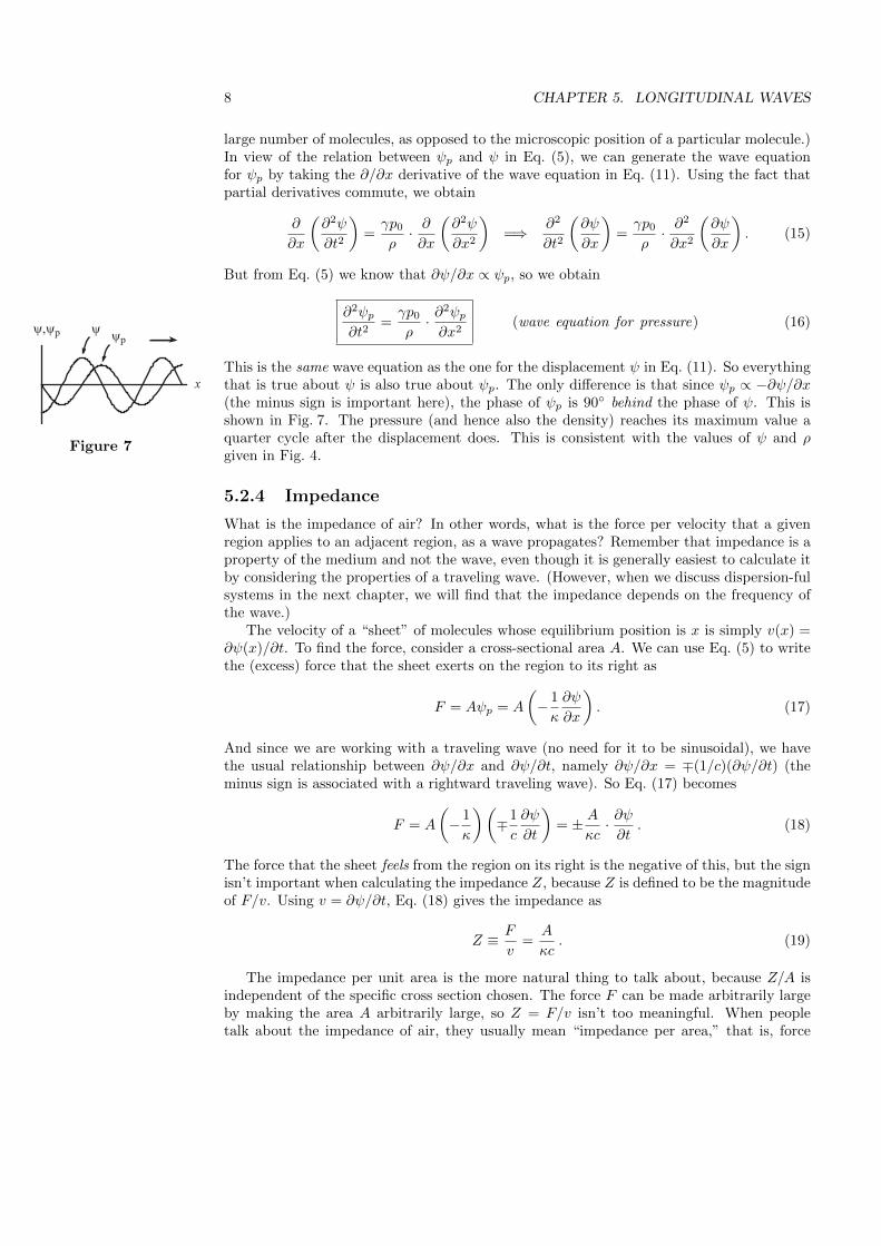
The lowest four standing waves for a clarinet are shown in Fig. 10 (described by the

(Pressure ψp)

λ=4L

λ=(4/3)L

λ=(4/5)L

λ=(4/7)L

L

Figure 10

pressure waves, which is customary). The wavelengths are 4L, 4L/3, 4L/5, 4L/7, etc. Thefrequencies are inversely proportional to the wavelengths, because νλ = c =⇒ ν ∝ 1/λ. Sothe frequencies are in the ratio of 1 : 3 : 5 : 7 : · · ·. These notes are very far apart. For anopen/open pipe like a flute, the wavelengths are 2L, 2L/2, 2L/3, 2L/4, etc., which meansthat the frequencies are in the ratio of 1 : 2 : 3 : 4 : · · ·. These notes are also very far apart.So if a clarinet or a flute didn’t have any keys, you wouldn’t be able to play anywhere nearall of the notes in a standard scale.

Keys remedy this problem in the following way. If all the keys are closed, then we simplyhave a pipe. But if a given key is open, then this forces the pressure wave to have a nodeat that point, because the pressure must match up with the atmospheric pressure there. Sowe have essentially shortened the pipe by creating an effectively open end at the locationof the open key. With many keys, this allows for many different effective pipe lengths, andhence many different notes. And also many different ways to play a given note. If we havea particular standing wave in the instrument, and if we then open a key at the location ofa (pressure) node, then this doesn’t change anything, so we get the same note.

What about a trumpet, which has only three valves? It’s a bit complicated, but theconical shape (at least near the end) has the effect of making the frequencies be closertogether (and also higher). And the mouthpiece helps too. The end result (if done properly)is that the frequencies are in the ratio 2 : 3 : 4 : 5 : 6 : · · · (for some reason, the 1 is missing)instead of the 1 : 3 : 5 : 7 : · · · ratios for the closed/open case in Fig. 10. This is indeed theratio of the frequencies of the notes (C,G,C,E,G,. . . ) that can be be played on a trumpetwithout pressing down any valves. The valves then change the length of the pipe in astraightforward manner.

The flared bell of a trumpet has the effect (compared with a cylinder of the same length)of raising the low notes more than the high notes, because the long wavelengths (low notes)can’t follow the bell as easily, so they’re reflected sooner than the short wavelengths.5 Thelonger wavelengths therefore effectively see a shorter pipe. However, another effect of the bellis that because the short wavelengths follow it so easily (right out to the outside atmosphericpressure), there isn’t much reflection for these waves, so it’s harder to get a standing wave.The high notes are therefore less well defined, and thus blend together (which is quite evidentif you’ve ever heard a trumpet player screeching away in the high register).

Everything you ever wanted to know about the physics of musical instruments can befound on this website: http://www.phys.unsw.edu.au/music

4The third option in Fig. 9, the closed/closed pipe, isn’t too conducive to making music. Such aninstrument couldn’t have any keys, because they provide openings to the outside world. And furthermore,you couldn’t blow into one like in reed or brass instrument, because there would be no place for the air tocome out. And you can’t blow across an opening like in a flute, because that’s an open end.

5The fact that the shorter wavelengths (high notes) can follow the bell is the same effect as in the“Gradually changing string density” impedance-matching example we discussed in Section 4.3.2.

longitudinal waves - harvard university2 chapter 5. longitudinal waves for a transverse wave, ˆ is...

Documents