loop coproducts onbg12 -...
TRANSCRIPT
THE BV ALGEBRA IN STRING TOPOLOGY OF CLASSIFYING
SPACES
KATSUHIKO KURIBAYASHI AND LUC MENICHI
Abstract. For almost any compact connected Lie group G and any field Fp,
we compute the Batalin-Vilkovisky algebra H∗+dim G(LBG; Fp) on the loopcohomology of the classifying space introduced by Chataur and the second
author. In particular, if p is odd or p = 0, this Batalin-Vilkovisky algebra isisomorphic to the Hochschild cohomology HH∗(H∗(G), H∗(G)). Over F2, suchisomorphism of Batalin-Vilkovisky algebras does not hold when G = SO(3)or G = G2. Our elaborate considerations on the signs in string topology ofthe classifying spaces give rise to a general theorem on graded homologicalconformal field theory.
1. Introduction
Let M be a closed oriented smooth manifold and let LM denote the space offree loops on M . Chas and Sullivan [4] have defined a product on the homology ofLM , called the loop product, H∗(LM)⊗H∗(LM)→ H∗−dim M (LM). They showedthat this loop product, together with the homological BV-operator ∆ : H∗(LM)→H∗+1(LM), make the shifted free loop space homologyH∗(LM) := H∗+dim M (LM)into a Batalin-Vilkovisky algebra, or BV algebra. Over Q, when M is simply-connected, this BV algebra can be computed using Hochschild cohomology [11].In particular, if M is formal over Q, there is an isomorphism of BV algebras be-tweenH∗(LM) andHH∗(H∗(M ;Q), H∗(M ;Q)), the Hochschild cohomology of thesymmetric Frobenius algebra H∗(M ;Q). Over a field Fp, if p 6= 0, this BV alge-bra H∗(LM) is hard to compute. It has been computed only for complex Stiefelmanifolds [41], spheres [34], compact Lie groups [20, 35] and complex projectivespaces [5, 18].
Let G be a connected compact Lie group of dimension d and let BG its clas-sifying space. Motivated by Freed-Hopkins-Teleman twisted K-theory [13] and bya structure of symmetric Frobenius algebra on H∗(G), Chataur and the secondauthor [6] have proved that the homology of the free loop space LBG with coeffi-cients in a field K admits the structure of a d-dimensional homological conformalfield theory (More generally, if G acts smoothly on M , Behrend, Ginot, Noohiand Xu [1, Theorem 14.2] have proved that H∗(L(EG ×G M)) is a (d − dim M)-homological conformal field theory.). In particular, the operation associated witha cobordism connecting one dimensional manifolds called the pair of pants, de-fines a product on the cohomology of LBG, called the dual of the loop coproduct,H∗(LBG) ⊗ H∗(LBG) → H∗−d(LBG). Chataur and the second author showedthat the dual of the loop coproduct, together with the cohomological BV-operator
2010 Mathematics Subject Classification: 55P50, 81T40, 55R35Key words and phrases. String topology, Batalin-Vilkovisky algebra, Classifying space.
Department of Mathematical Sciences, Faculty of Science, Shinshu University, Matsumoto,
Nagano 390-8621, Japan e-mail:[email protected] - UMR CNRS 6093, Universite d’Angers, 2 Bd Lavoisier, 49045 Angers, France
e-mail:[email protected] first author was partially supported by JSPS KAKENHI Grant Number 25287008.
1

2 KATSUHIKO KURIBAYASHI AND LUC MENICHI
∆ : H∗(LBG) → H∗−1(LBG), make the shifted free loop space cohomologyH∗(LBG) := H∗+d(LBG) into a BV algebra up to signs. Over F2, Hepworthand Lahtinen [19] have extended this result to non connected compact Lie groupand more difficult, they showed that this d-dimensional homological conformal fieldtheory, in particular this algebra H∗(LBG), has a unit. One of our result is to solvethe sign issues and to show that indeed, H∗(LBG) is a BV algebra (Corollary C.3).
In fact, one of the highlights in this manuscript is to show that more generally,the dual of a d-homological field theory has, after a d degree shift, a structure ofBV algebra (Theorems B.1 and C.1). Our elaborate considerations on the signsgive many explicit computations on H∗(LBG) as mentioned below. Surprisingly,these computations enable us to determine the signs on the product of the prop inTheorem B.1; that is, such local computations in string topology of BG give rise toa general theorem on graded homological conformal field theory.
In [30], Lahtinen computes some non-trivial higher operations in the structure ofthis d-dimensional homological conformal field theory on the cohomology of BG forsome compact Lie groups G. In this paper, we compute the most important partof this d-dimensional homological conformal field theory, namely the BV-algebraH∗(LBG;Fp) for almost any connected compact Lie group G and any field Fp. Ac-cording to our knowledge, this BV-algebra H∗(LBG;Fp) has never been computedon any example.
Very recently, Grodal and Lahtinen [15] have shown that the mod p cohomologyof a finite Chevalley group admits a module structure over this algebraH∗(LBG;Fp)where G is the p-compact group of C-rational points associated with the finitegroup. This result appears in the program to attack Tezuka question [45] aboutan isomorphism compatible with the cup products between this group cohomologyand this free loop space cohomology of BG. Thus our explicit computations arealso strongly relevant to the program.
Our method is completely different from the methods used to compute the BValgebra H∗(LM) in the known cases recalled above. Suppose that the cohomologyalgebra of BG over Fp, H
∗(BG;Fp), is a polynomial algebra Fp[y1, ..., yN ] (fewconnected compact Lie groups do not satisfy this hypothesis). Then the cup producton H∗(LBG;Fp) was first computed by the first author in [28](see [24] for a quickcalculation). In his paper [42] entitled ”cap products in String topology”, Tamanoiexplains the relations between the cap product and the loop product on H∗(LM).Dually, in Theorem 2.2 entitled ”cup products in String topology of classifyingspaces”, we give the relations between the cup product on H∗(LBG) and the BValgebra H∗(LBG). Knowing the cup product on H∗(LBG), these relations givethe dual of the loop coproduct on H∗(LBG) (Theorem 3.1). But now, since thecohomological BV-operator ∆ (see appendix E) is a derivation with respect to thecup product, ∆ is easy to compute. So finally, on H∗(LBG), we have computed atthe same time, the cup product and the BV-algebra structure. This has never bedone for the BV algebra H∗(LM).
If there is no top degree Steenrod operation Sq1 on H∗(BG;F2), if p is odd orp = 0, applying Theorem 3.1, we give an explicit formula for the dual of the loopcoproduct ⊙ in Theorem 4.1 and we show in Theorem 6.2 that there is an isomor-phism of BV algebras between H∗(LBG;Fp) and HH
∗(H∗(G;Fp), H∗(G;Fp)), theHochschild cohomology of the symmetric Frobenius algebra H∗(G;Fp).

THE BV ALGEBRA IN STRING TOPOLOGY OF CLASSIFYING SPACES 3
The case p = 2 is more intriguing. When p = 2, we don’t give in general anexplicit formula for the dual of the loop coproduct ⊙ (however, see Theorem 5.4 fora general equation satisfied by ⊙). But for a given compact Lie group G, applyingTheorem 3.1, we are able to give an explicit formula. As examples, in this paper, wecompute the dual of the loop coproduct when G = SO(3) (Theorem 5.7) or G = G2
(Theorem 5.1). We show (Theorem 6.3) that the BV algebrasH∗(LBSO(3);F2) andHH∗(H∗(SO(3);F2), H∗(SO(3);F2)), the Hochschild cohomology of the symmet-ric Frobenius algebra H∗(SO(3);F2), are not isomorphic although the underlyingGerstenhaber algebras are isomorphic. Such curious result was observed in [34] forthe Chas-Sullivan BV algebras H∗(LS
2;F2).However, for any connected compact Lie group such that H∗(BG;Fp), is a poly-
nomial algebra, we show (Corollary 4.3 and Theorem 5.8) that as graded algebras
H∗(LBG;Fp) ∼= H∗(G;Fp)⊗H∗(BG;Fp) ∼= HH∗(H∗(G;Fp), H∗(G;Fp)).
Such isomorphisms of Gerstenhaber algebras should exist (Conjecture 6.1).We give now the plan of the paper:Section 2: We carefully recall the definition of the loop product and of the loop
coproduct insisting on orientation (Theorem 2.1). Theorem 2.2 mentioned above isproved.
Section 3: WhenH∗(X) is a polynomial algebra, following [28] or [24], we give thecup product on H∗(LX). Therefore (Theorem 3.1) the dual of the loop coproductis completely given by Theorems 2.1 and 2.2.
Section 4 is devoted to the simple case when the characteristic of the field isdifferent from two or when there is no top degree Steenrod operation.
Section 5: The field is F2. We give some general properties of the dual of theloop coproduct (Lemma 5.3, Theorem 5.4). In particular, we show that it has aunit (Theorem 5.5). As examples, we compute the dual of the loop coproduct onH∗(LBSO(3);F2) and on H∗(LBG2;F2) (Theorems 5.7 and 5.1). Up to an iso-morphism of graded algebras, H∗(LX ;F2) is just the tensor product of algebrasH∗(X ;F2) ⊗ H−∗(ΩX ;F2) = F2[V ] ⊗ Λ(sV )∨ (Theorem 5.8). As examples, wecompute the BV-algebra H∗+3(LBSO(3);F2) ∼= Λ(u−1, u−2) ⊗ F2[v2, v3] (Theo-rem 5.13) and the BV-algebra H∗+14(LBG2;F2) ∼= Λ(u−3, u−5, u−6)⊗F2[v4, v6, v7](Theorem 5.14).
Section 6: After studying the formality and the coformality of BG, we comparethe associative algebras, the Gerstenhaber algebras, the BV-algebrasH∗(LBG) andHH∗(H∗(G), H∗(G)) under various hypothesis.
Section 7: In this last section independent of the rest of the paper, we show thatthe loop product on H∗(LBG;Fp) is trivial if and only if the inclusion of the fibreι : ΩBG → LBG induces a surjective map in cohomology if and only if H∗(BG;Fp)is a polynomial algebra if and only if BG is Fp-formal (when p is odd).
Appendix A: We solve some sign problems in the results of Chataur and thesecond author. In particular, we correct the definition of integration along the fibreand the main dual theorem of [6] concerning the prop structure on H∗(LX).
Appendix B: ThereforeH∗(LX) is equipped with a graded associative and gradedcommutative product ⊙.
Appendix C: In fact, H∗(LX) equipped with ⊙ and the BV-operator ∆ is aBV-algebra since the BV identity arises from the lantern relation.
Appendix D: This BV identity comes from seven equalities involving Dehn twistsand the prop structure on the mapping class group.

4 KATSUHIKO KURIBAYASHI AND LUC MENICHI
Appendix E:We compare different definitions of the BV-operator ∆ : H∗(LX)→H∗−1(LX).
Appendix F: We compute the Gerstenhaber algebra structure on the Hochschildcohomology HH∗(S(V ), S(V )) of a free commutative graded algebra S(V ) (The-orem F.3). In particular, we give the BV-algebra structure on the Hochschildcohomology HH∗(Λ(V ),Λ(V )) of a graded exterior algebra Λ(V ).
2. The dual of the Loop coproduct
In this paper, all the results are stated for simplicity for a connected compactLie group G. But they are also valid for an exotic p-compact group. Indeed, follow-ing [6], we only require that G is a connected topological group (or a pointed loopspace) with finite dimensional cohomology H∗(G;Fp). This is the main differencewith [19], where Hepworth and Lahtinen require the smoothness of G.
Let K be a field. Let X be a simply-connected space satisfying the condition thatH∗(ΩX ;K) is of finite dimension. Then there exists a unique integer d such thatHi(ΩX ;K) = 0 for i > d and Hd(ΩX ;K) ∼= K. In order to describe our results, wefirst recall the definitions of the product Dlcop on H∗+d(LX ;K) and of the loopproduct on H∗−d(LX ;K) defined by Chataur and the second author in [6].
Let F be the pair of pants regarded as a cobordism between one ingoing circleand two outgoing circles. The ingoing map in : S1 → F and outgoing map out :S1
∐S1 → F give the correspondence
LX map(F,X)map(in,X)oooo map(out,X)// // LX × LX
where map(in,X) and map(out,X) are orientable fibrations. After orienting them,the integration along the fibre induces a map in cohomology
map(in,X)! : H∗+d(map(F,X))→ H∗(LX)
and a map in homology
map(out,X)! : H∗(LX)⊗2 → H∗+d(map(F,X)).
See appendix A for the definition of the integration along the fibre. By definition,the loop product is the composite
H∗(map(in,X))map(out,X)! : Hp−d(LX)⊗Hq−d(LX)→ Hp+q−d(map(F,X))
→ Hp+q−d(LX).
By definition, the dual of the loop coproduct, denoted Dlcop, is the composite
map(in,X)!H∗(map(out,X)) : Hp+d(LX)⊗Hq+d(LX)→ Hp+q+2d(map(F,X))
→ Hp+q+d(LX).
The pair of pants F is the mapping cylinder of c∐π : S1
∐(S1
∐S1) → S1 ∨ S1
where c : S1 → S1∨S1 is the pinch map and π : S1∐S1 → S1∨S1 is the quotient
map. Therefore the wedge of circles S1 ∨ S1 is a strong deformation retract of the
pair of pants F . The retract r : F≈
։ S1 ∨ S1 corresponds to lower his pants andtuck up his trouser legs at the same time:

THE BV ALGEBRA IN STRING TOPOLOGY OF CLASSIFYING SPACES 5
Figure 1. the homotopy between the pairs of pants and the figure eight.
Thus we have the commutative diagram
LX map(F,X)map(out,X) //map(in,X)oo LX×2
LX ×X LX
Comp
hh q
66map(r,X)≈
OO
where Comp is the composition of loops and q is the inclusion. If X was a closedmanifold M of dimension d, Comp and q would be embeddings. And the Chas-Sullivan loop product is the composite
H∗(Comp)q! : Hp+d(LM)⊗Hq+d(LM)→ Hp+q+d(LM×MLM))→ Hp+q+d(LM).
while the dual of the loop coproduct is the composite
Comp! H∗(q) : Hp−d(LM)⊗Hq−d(LM)→ Hp+q−2d(LM×MLM)→ Hp+q−d(LM).
Therefore although Comp and q are not fibrations, by an abuse of notation, some-times, we will say that in the case of string topology of classifying spaces [6], the
loop product on H∗−d(LX) is still H∗(Comp) q! while Dlcop is Comp! H∗(q).The shifted cohomology H∗(LX) := H∗+d(LX) together with the dual of the
loop coproduct Dlcop defined by Chataur and the second author in [6] is a Batalin-Vilkovisky algebra, in particular a graded commutative associative algebra, onlyup to signs for two reasons:
-First, the integration along the fibre defined in [6] as usually does not satisfy theusual property with respect to the product. We have corrected this sign mistakeof [6] in appendix A.
-Second, as explained in appendix A, this is also due to the non-triviality of theprop detH1(F, ∂out;Z)⊗d (if d is odd).
Nevertheless, we show TheoremC.1. In particular, we have thatH∗(LX) equippedwith the operator ∆ induced by the action of the circle on LX (See our definition inappendix E) is a Batalin-Vilkovisky algebra with respect to the product ⊙ definedby
a⊙ b = (−1)d(d−|a|)Dlcop(a⊗ b)
for a⊗ b ∈ H∗(LX)⊗H∗(LX); see Corollary C.3 below.In order to investigate Dlcop more precisely, we need to know how the fibration
map(in,X) is oriented. As explained in [6, section 11.5], we have to choose a
pointed homotopy equivalence f : F/∂in≈→ S1. Then the fibre map∗(F/∂in, X) of
map(in,X) is oriented by the composite
τ Hd(map∗(f,X)) : Hd(map∗(F/∂in, X))→ Hd(ΩX)→ K.

6 KATSUHIKO KURIBAYASHI AND LUC MENICHI
where τ is the orientation on ΩX that we choose. In this paper, we choose f suchthat we have the following homotopy commutative diagram
map∗(F/∂in, X)incl // map(F,X)
ΩX
map∗(f,X) ≈
OO
j// LX ×X LX
map(r,X)≈
OO
where incl is the inclusion of the fibre of map(in,X) and j is the map defined byj(ω) = (ω, ω−1).
Theorem 2.1. Let ι : ΩX → LX be the inclusion of pointed loops into free loops.Let S be the antipode of the Hopf algebra H∗(ΩX). Let τ : Hd(ΩX) → K be thechosen orientation on ΩX. Let a ∈ Hp(LX) and b ∈ Hq(LX) such that p+ q = d.
Then with the above choice of pointed homotopy equivalence f : F/∂in≈→ S1,
a⊙ b = (−1)d(d−p)τ (Hp(ι)(a) ∪ S Hq(ι)(b)) 1H∗(LX).
Proof. Let Fincl→ E
proj։ B be an oriented fibration with orientation τ : Hd(F )→ K.
By definition or by naturality with respect to pull-backs, the integration along thefibre proj ! is in degree d the composite
Hd(E)Hd(incl)→ Hd(F )
τ→ K
η→ H0(B)
where η is the unit ofH∗(B). Therefore Dlcop is given by the commutative diagram
Hd(LX × LX)
Hd map(out,X)
uu
Hd(q)
Hd(ι×ι)
((
Hd(map(F,X))Hd map(r,X)
//
Hd(incl)
map(in,X)!
&&
Hd(LX ×X LX)
Hd(j)
Hd(incl)// Hd(ΩX × ΩX)
Hd(Id×Inv)
Hd(map∗(F/∂in))
Hd map∗(f,X)
// Hd(ΩX)
τ
Hd(ΩX × ΩX)Hd(∆)
oo
H0(LX) Kηoo
where incl : ΩX × ΩX → LX ×X LX is the inclusion and Inv : ΩX → ΩX mapsa loop ω to its inverse ω−1. Therefore
Dlcop(a⊗ b) = τ (Hp(ι)(a) ∪ S Hq(ι)(b)) 1H∗(LX).
We define a bracket , on H∗(LX) with the product ⊙ and the Batalin-Vilkovisky operator ∆ : H∗(LX)→ H∗−1(LX) by
a, b = (−1)|a|∆(a⊙ b)− (−1)|a|∆(a)⊙ b− a⊙∆(b)
for a, b in H∗(LX). By Theorem C.3, this bracket is exactly a Lie bracket. Thefollowing theorem is analogous for string topology of classifying spaces [6] to thetheorems of Tamanoi in [42] for Chas-Sullivan string topology [4]. This analogy isquite surprising and complete. For our calculations, in the rest of the paper, we
THE BV ALGEBRA IN STRING TOPOLOGY OF CLASSIFYING SPACES 7
use only parts (1), (2) and (3) of this theorem. Let ev : LX ։ X be the evaluationmap defined by ev(γ) = γ(0) for γ ∈ LX .
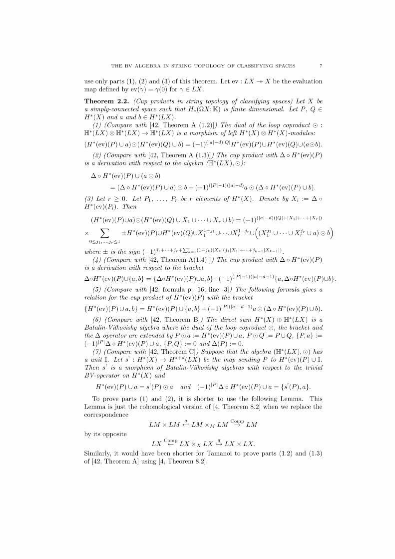
Theorem 2.2. (Cup products in string topology of classifying spaces) Let X bea simply-connected space such that H∗(ΩX ;K) is finite dimensional. Let P , Q ∈H∗(X) and a and b ∈ H∗(LX).
(1) (Compare with [42, Theorem A (1.2)]) The dual of the loop coproduct ⊙ :H∗(LX)⊗H∗(LX)→ H∗(LX) is a morphism of left H∗(X)⊗H∗(X)-modules:
(H∗(ev)(P ) ∪ a)⊙(H∗(ev)(Q) ∪ b) = (−1)(|a|−d)|Q|H∗(ev)(P )∪H∗(ev)(Q)∪(a⊙b).
(2) (Compare with [42, Theorem A (1.3)]) The cup product with ∆ H∗(ev)(P )is a derivation with respect to the algebra (H∗(LX),⊙):
∆ H∗(ev)(P ) ∪ (a⊙ b)
= (∆ H∗(ev)(P ) ∪ a)⊙ b+ (−1)(|P |−1)(|a|−d)a⊙ (∆ H∗(ev)(P ) ∪ b).
(3) Let r ≥ 0. Let P1, . . . , Pr be r elements of H∗(X). Denote by Xi := ∆ H∗(ev)(Pi). Then
(H∗(ev)(P )∪a)⊙(H∗(ev)(Q) ∪X1 ∪ · · · ∪Xr ∪ b) = (−1)(|a|−d)(|Q|+|X1|+···+|Xr |)
×∑
0≤j1,...,jr≤1
±H∗(ev)(P )∪H∗(ev)(Q)∪X1−j11 ∪· · ·∪X1−jr
r ∪((Xj1
1 ∪ · · · ∪Xjrr ∪ a)⊙ b
)
where ± is the sign (−1)j1+···+jr+∑r
k=1(1−jk)|Xk|(j1|X1|+···+jk−1|Xk−1|).(4) (Compare with [42, Theorem A(1.4) ]) The cup product with ∆ H∗(ev)(P )
is a derivation with respect to the bracket
∆H∗(ev)(P )∪a, b = ∆H∗(ev)(P )∪a, b+(−1)(|P |−1)(|a|−d−1)a,∆H∗(ev)(P )∪b.
(5) (Compare with [42, formula p. 16, line -3]) The following formula gives arelation for the cup product of H∗(ev)(P ) with the bracket
H∗(ev)(P )∪ a, b = H∗(ev)(P )∪ a, b+(−1)|P |(|a|−d−1)a⊙ (∆ H∗(ev)(P )∪ b).
(6) (Compare with [42, Theorem B]) The direct sum H∗(X) ⊕ H∗(LX) is aBatalin-Vilkovisky algebra where the dual of the loop coproduct ⊙, the bracket andthe ∆ operator are extended by P ⊙ a := H∗(ev)(P )∪a, P ⊙Q := P ∪Q, P, a :=(−1)|P |∆ H∗(ev)(P ) ∪ a, P,Q := 0 and ∆(P ) := 0.
(7) (Compare with [42, Theorem C]) Suppose that the algebra (H∗(LX),⊙) hasa unit I. Let s! : H∗(X) → H∗+d(LX) be the map sending P to H∗(ev)(P ) ∪ I.Then s! is a morphism of Batalin-Vilkovisky algebras with respect to the trivialBV-operator on H∗(X) and
H∗(ev)(P ) ∪ a = s!(P )⊙ a and (−1)|P |∆ H∗(ev)(P ) ∪ a = s!(P ), a.
To prove parts (1) and (2), it is shorter to use the following Lemma. ThisLemma is just the cohomological version of [4, Theorem 8.2] when we replace thecorrespondence
LM × LMq← LM ×M LM
Comp→ LM
by its opposite
LXComp← LX ×X LX
q→ LX × LX.
Similarly, it would have been shorter for Tamanoi to prove parts (1.2) and (1.3)of [42, Theorem A] using [4, Theorem 8.2].

8 KATSUHIKO KURIBAYASHI AND LUC MENICHI
Lemma 2.3. Let a =∑a1 ⊗ a2 ∈ H∗(LX × LX) and A ∈ H∗(LX) such that
H∗(Comp)(A) = H∗(q)(a). Then for any z1, z2 ∈ H∗(LX),
A ∪ (z1 ⊙ z2) =∑
(−1)(|z1|−d)|a2|(a1 ∪ z1)⊙ (a2 ∪ z2).
Proof. The integration along the fibre, Comp!, is a morphism of left H∗(LX)-modules with the correct signs (See our definition of integration along the fibre incohomology in appendix A). Therefore
Comp!(H∗(Comp)(A) ∪ y) = (−1)d|A|A ∪ Comp!(y).
Let z := z1 ⊗ z2 ∈ H∗(LX × LX). Since H∗(q) is a morphism of algebras,
(−1)d|A|Dlcop(a ∪ z) = (−1)d|A|Comp! H∗(q)(a ∪ z)
= (−1)d|A|Comp!(H∗(Comp)(A) ∪H∗(q)(z))
= A ∪ Comp! H∗(q)(z) = A ∪Dlcop(z) .
Then the previous equation is
A∪(−1)d(|z1|−d)z1⊙z2 =∑
(−1)d(|a1|+|a2|)(−1)d(|a1|+|z1|−d)(−1)|a2||z1|(a1∪z1)⊙(a2∪z2)
Proof of Theorem 2.2. (1) We have the commutative diagram
LX
ev''
LX ×X LXCompoo q //
LX × LX
ev× ev
Xδ
// X ×X
Therefore by applying Lemma 2.3 to a := H∗(ev× ev)(P ⊗Q), A := H∗(δev)(P ⊗Q), z1 := a and z2 := b, we obtain (1).
(2) By [42, Proof of Theorem 4.2 (4.5)]
Comp∗(∆ H∗(ev)(P )) = H∗(q)(∆ H∗(ev)(P )× 1 + 1×∆ H∗(ev)(P )).
So we can apply Lemma 2.3 to a := ∆ H∗(ev)(P ) × 1 + 1 ×∆ H∗(ev)(P ) andA := ∆ H∗(ev)(P ). We obtain (2).
(3) The case r = 0 is just (1). Now, by induction on r,
(H∗(ev)(P )∪a)⊙(H∗(ev)(Q)∪X1∪· · ·∪Xr−1∪(Xr∪b)) = (−1)(|a|−d)(|Q|+|X1|+···+|Xr−1|)×∑
0≤j1,...,jr−1≤1
±H∗(ev)(P )∪H∗(ev)(Q)∪X1−j11 ∪· · ·∪X
1−jr−1
r−1 ∪((Xj1
1 ∪ · · · ∪Xjr−1
r−1 ∪ a)⊙ (Xr ∪ b)
)
But by (2),(Xj1
1 ∪ · · · ∪Xjr−1
r−1 ∪ a)⊙ (Xr ∪ b) =
1∑
jr=0
(−1)|Xr|(|a|−d)+jr+(1−jr)|Xr |∑r−1
l=1 jl|Xl|X1−jrr ∪
((Xj1
1 ∪ · · · ∪Xjrr ∪ a
)⊙ b
)
(4) By using the formula (2), the same argument as in [42, Proof of Theorem4.5] deduces the derivation formula on the bracket.

THE BV ALGEBRA IN STRING TOPOLOGY OF CLASSIFYING SPACES 9
(5) Again, the arguments are identical as those given by Tamanoi: see [42, endof proof of Theorem 4.7].
(6) As explained in [42, proof of Theorem 4.7] by Tamanoi, (2), (4) and (5)are equivalent to the Poisson and Jacobi identities in the Gerstenhaber algebraH∗(X) ⊕ H∗(LX). By definition of the bracket, this Gerstenhaber algebra is aBatalin-Vilkovisky algebra: see [42, proof of Theorem 4.8].
(7) Since H∗+d(LX) is a H∗(X)-algebra (formula (1) of Theorem 2.2), the maps! : H∗(X)→ H∗+d(LX), P 7→ H∗(ev)(P )∪I, is a morphism of unital commutativegraded algebras (we denote this map s! because this map should coincide with someGysin map of the trivial section s : X → LX [6]. Indeed, by H∗(LX)-linearity,s!(P ) = s! H∗(s) H∗(ev)(P ) = (−1)d|P |H∗(ev)(P ) ∪ s!(1).
Since the cup product with ∆ H∗(ev)(P ) is a derivation with respect to thedual of the loop coproduct, ∆ H∗(ev)(P ) ∪ I = 0. Since H∗(LX) is a Batalin-Vilkovisky algebra, ∆(I) = 0. Therefore, since ∆ is a derivation with respect to thecup product,
∆(s!(P )) = ∆ H∗(ev)(P ) ∪ I+ (−1)|P |H∗(ev)(P ) ∪∆(I) = 0 + 0.
Now we can conclude using the same arguments as in [42, proof of Theorem 5.1].
Remark 2.4. Suppose that the algebraH∗(LX) is generated byH∗(X) and ∆(H∗(X)).Then by formula (3) of Theorem 2.2 in the case b = 1, we see that the dual of theloop coproduct ⊙ is completely given by the cup product, by the ∆ operator andby its restriction on H∗(LX)⊗ 1. In the following section, we show that this is thecase when H∗(X) is a polynomial (see remark 3.2).
3. The cup product on free loops and the main theorem
Let X be a simply-connected space with polynomial cohomology: H∗(X) is apolynomial algebra K[y1, ..., yN ]. The cup product on the free loop space cohomol-ogy H∗(LX ;K) was first computed by the first author in [28, Theorem 1.6]. Wenow explain how to recover simply this computation following [24, p. 648].
Let σ : H∗(X) → H∗−1(ΩX) be the suspension homomorphism and σ(yi) bethe suspension image of yi. By Borel theorem [38, Chapter VII. Corollary 2.8(2)](which can be easily proved using the Eilenberg-Moore spectral sequence associatedto the path fibration ΩX → PX ։ X since E∗,∗
2∼= Λ(σ(y1), . . . , σ(yN ))),
H∗(ΩX ;K) = ∧(σ(y1), . . . , σ(yN ))
where ∧σ(yi) denotes an algebra with simple system of generators σ(yi) (Herean algebra with simple system of generators xi is a graded commutative algebra,denoted ∧xi, such that the products of the form xi1xi2 . . . xir with 1 ≤ i1 < i2 <· · · < ir ≤ N and r ≥ 0 form a linear basis of the algebra [38, Definition p. 367]).If ch(K) 6= 2, ∧σ(yi) is just the exterior algebra Λσ(yi).
Let ∆ : H∗(LX) → H∗−1(LX) be the operator induced by the action of thecircle on LX (See appendix E). Let D := ∆ H∗(ev) denotes the module deriva-tion of the first author in [28]. Since ∆ is a derivation with respect to the cupproduct, D is a (H∗(ev), H∗(ev))-derivation [28, Proposition 3.3]. Since ∆ andH∗(ev) commutes with the Steenrod operations, D also [28, Proposition 3.3]. Sincethe composite H∗(ι) D is the suspension homomorphism σ [24, Proposition 2(1)],H∗(ι) is surjective and so by Leray-Hirsch theorem,
H∗(LX ;K) = H∗(X)⊗ ∧ (D(y1), . . . ,D(yN ))

10 KATSUHIKO KURIBAYASHI AND LUC MENICHI
as H∗(X)-algebra. Modulo 2, it follows from above that H∗(LX ;F2) is the poly-nomial algebra
F2[H∗(ev)(yi),Dyi]
quotiented by the relations
(Dyi)2 = D(Sq|yi|−1yi).
In particular, we have ∆(H∗(ev)(yi)) = Dyi and ∆(Dyi) = 0 since ∆ ∆ = 0.Therefore, we know the cup product and the ∆ operator on H∗(LX ;K). Thefollowing theorem claims that we also know the dual of the loop coproduct.
Theorem 3.1. Let X be a simply-connected space such that H∗(X ;K) is thepolynomial algebra K[y1, . . . , yN ]. Denote again by yi, the element of H∗(LX),H∗(ev)(yi), and by xi, ∆ H
∗(ev)(yi). Often, the cup product a∪ b on H∗(LX) isnow simply denoted ab. With respect to this cup product, as algebras
H∗(LX) = K[y1, . . . , yN ]⊗ ∧(x1, . . . , xN ).
Let d be the degree of x1 . . . xN . Then the dual of the loop coproduct
⊙ : Hi(LX)⊗Hj(LX)→ Hi+j−d(LX)
is given inductively (see remark 3.2) by the following four formulas(1) For any a and b ∈ H∗(LX), ∀1 ≤ i ≤ N ,
a⊙ xib = (−1)|xi|(|a|−d)xi(a⊙ b)− (−1)d|xi|axi ⊙ b
(2) Let i1, . . . , il and j1, . . . , jm be two disjoint subsets of 1, . . . , N such
that i1, . . . , il ∪ j1, . . . , jm = 1, . . . , N. If we orient τ : Hd(ΩX)∼=→ K by
τ H∗(ι)(x1 . . . xN ) = 1 then
xi1 . . . xil ⊙ xj1 . . . xjm = (−1)Nm+mε
where ε is the signature of the permutation
(1 . . . l +mi1 . . . ilj1 . . . jm
).
(3) Let i1, . . . , il and j1, . . . , jm be two disjoint subsets of 1, . . . , N suchthat i1, . . . , il ∪ j1, . . . , jm 6= 1, . . . , N. Then
xi1 . . . xil ⊙ xj1 . . . xjm = 0.
(4) ⊙ is a morphism of left H∗(X) ⊗H∗(X)-modules: for P , Q ∈ H∗(X) anda, b ∈ H∗(LX), one has (−1)|Q|(|a|−d)Pa⊙Qb = PQ(a⊙ b).
Proof. Note that if yi is of odd degree then 2 = 0 in K. (1) and (4) are particularcases of (1) and (2) of Theorem 2.2. Since xi1 . . . xil ⊗ xj1 . . . xjm is of degree lessthan d, for degree reasons, we have (3).
(2) Since H∗(ι)(xi) = H∗(ι) ∆ H∗(ev)(yi) is the suspension of yi, denotedσ(yi), by Theorem 2.1,
xi1 . . . xil ⊙ xj1 . . . xjm = (−1)Nmτ (σ(yi1 ) . . . σ(yil) ∪ S(σ(yj1 ) . . . σ(yjm )) 1.
Since σ(yi) is a primitive element, S(σ(yi)) = −σ(yi). Since also the antipodeS : H∗(ΩX)→ H∗(ΩX) is a morphism of commutative graded algebras,
xi1 . . . xil ⊙ xj1 . . . xjm = (−1)Nm+mετ(σ(y1) . . . σ(yN )).

THE BV ALGEBRA IN STRING TOPOLOGY OF CLASSIFYING SPACES 11
Remark 3.2. We explain now why the four formulas of Theorem 3.1 determine in-ductively the dual of the loop coproduct ⊙. For P ∈ H∗(X) and i1, . . . , il a strictsubset of 1, . . . , N, by (2), (3) and (4), Pxi1 . . . xil⊙1 = 0 and Px1 . . . xN⊙1 = P .Therefore, we know the restriction of ⊙ on H∗(LX)⊗1. Since the algebra H∗(LX)is generated by H∗(X) and ∆(H∗(X)), the product ⊙ is now given inductively by(1) and (4) (see remark 2.4).
The restriction of ⊙ : H∗(LX) ⊗ 1 → H∗(X) looks similar to the intersectionmorphism ι! : H∗(LM) → H∗(ΩM) for a manifold M given by the loop productwith the constant pointed loop.
4. Case p odd or no Sq1
Let Sq1 be the operatorH∗(BG;F2)→ H∗(BG;F2) defined by Sq1(x) = Sqdegx−1x
for x ∈ H∗(BG;F2).Suppose that H∗(BG;K) is a polynomial algebra K[y1, . . . , yN ] and that
(H) : Sq1 ≡ 0 on H∗(BG) if K = F2 or the characteristic of K isdifferent from 2 (Since Sq1(PQ) = P 2Sq1(Q) + Sq1(P )Q
2, it suffices to check thatSq1(yi) = 0 for all i).
Then it follows from Section 3 (or [26, Remark 3.4]) that
H∗(LBG;K) = ∧(x1, . . . , xN )⊗K[y1, . . . , yN ]
as an algebra where xi := ∆ H∗(ev)(yi). Then we have
Theorem 4.1. Under the hypothesis (H), an explicit form of the dual of the loopcoproduct ⊙ : H∗(LBG;K)⊗H∗(LBG;K)→ H∗−dimG(LBG;K) is given by
xi1 · · ·xila⊙ xj1 · · ·xjmb = (−1)ε′+ε+m+u+lu+Nmxk1 · · ·xku
ab
if i1, ...il ∪ j1, ..., jm = 1, ..., N and xi1 · · ·xila ⊙ xj1 · · ·xjmb = 0 otherwise,where i1, ...il ∩ j1, ..., jm = k1, .., ku, a, b ∈ H
∗(BG),
(−1)ε = sgn
(j1.... .... .... ...jmk1...kuj1...k1...ku...jm
)and (−1)ε
′
= sgn
(i1...ilj1...k1...ku...jm1.... .... .... ...N
).
Over R, [1, 17.23] has the same formula without any signs for their dual hiddenloop product ⋆ on H∗([G/G]). With our signs, ⊙ is graded associative and gradedcommutative (Corollary B.3). In [1, 17.23], ⋆ is commutative but not graded com-mutative. For example, by [1, 17.23],
x1 . . . xN−1 ⋆ x2 . . . xN = x2 . . . xN = x2 . . . xN ⋆ x1 . . . xN−1
although x1 . . . xN−1 and x2 . . . xN are of odd degree in H∗+d(LBG).
Proof of Theorem 4.1. By (4) of Theorem 3.1 to prove Theorem 4.1, it suffices toshow that the formula for the element xi1 · · ·xil ⊗ xj1 · · ·xjm , namely in the casewhere a = b = 1.
Since x2k1= 0, xi1 · · ·xilxk1 ⊙ xj1 · · · xk1 · · ·xjm = 0. So by (1) of Theorem 3.1,
xi1 · · ·xil ⊙ xj1 · · ·xjm
= (−1)|xk1|(|xi1 ···xil
xj1 ···xk1|−d)xk1(xi1 · · ·xil ⊙ xj1 · · · xk1 · · ·xjm).

12 KATSUHIKO KURIBAYASHI AND LUC MENICHI
By induction on u,
xi1 · · ·xil ⊙ xj1 · · ·xjm
= (−1)u(l−d)+εxk1 . . . xku(xi1 · · ·xil ⊙ xj1 · · · xk1 · · · xku
· · ·xjm).
By (2) and (3) of Theorem 3.1,
xi1 · · ·xil ⊙ xj1 · · · xk1 · · · xku· · ·xjm
=
(−1)N(m−u)+m−u+ε′ If i1, . . . , il ∪ j1, . . . , jm = 1, . . . , N,
0 otherwise.
Here x means that the element x disappears from the presentation.
Corollary 4.2. Under the hypothesis (H), the graded associative commutative al-gebra (H∗(LBG),⊙) of Corollary B.3 is unital.
Proof. We see that x1 · · ·xN is the unit. Theorem 4.1 yields that
x1 · · ·xN ⊙ xj1 · · ·xjmb =
sgn
(j1......jmj1......jm
)sgn
(1....N1....N
)(−1)m+m+mN+Nmxj1 · · ·xjmb.
xi1 · · ·xila⊙ x1 · · ·xN = sgn
(1.... .... .... ...N
i1...il1...i1...il...N
)
sgn
(i1...il1...i1...il...N1.... .... .... ...N
)(−1)N+l+l2+N2
xi1 · · ·xila.
Theorem 4.3. Under the hypothesis (H), H∗(LBG) = H∗+dim G(LBG;K) is iso-morphic as BV algebras to the tensor product of algebras
H∗(BG;K)⊗H−∗(G;K) ∼= K[y1, . . . , yN ]⊗ ∧(x∨1 , . . . , x∨N )
equipped with the BV-operator ∆ given by ∆(x∨i ∧ x∨j ) = ∆(yiyj) = ∆(x∨j ) =
∆(yi) = 0 for any i, j and
∆(yi ⊗ x∨j ) =
0 if i 6= j,1 if i = j.
Proof. Since H∗(G) is the Hopf algebra Λxi with xi = σ(yi) primitive, its dual isthe Hopf algebra Λx∨i . By Corollary B.3 and Corollary 4.2, we see that the shiftedcohomology H∗(LBG) is a graded commutative algebra with unit x1 . . . xN . Thisenables us to define a morphism of algebras Θ from
H∗(BG;K)⊗H−∗(G;K) = K[y1, · · · , yn]⊗ Λ(x∨1 , · · · , x∨N )
toH∗(LBG) = K[y1, · · · , yn]⊗ Λ(x1, · · · , xN )
by
Θ(1⊗x∨j ) = (−1)j−11⊗ (x1∧· · ·∧ xj ∧· · ·∧xN ) and Θ(a⊗1) = a⊗ (x1∧· · ·∧xN )
for any a in K[V ]. By induction on p, using Theorem 4.1, we have
Θ(a⊗ (x∨j1 ∧ · · · ∧ x∨jp)) = ±a⊗ (x1 ∧ · · · ∧ xj1 ∧ · · · ∧ xjp ∧ · · · ∧ xN )
THE BV ALGEBRA IN STRING TOPOLOGY OF CLASSIFYING SPACES 13
for any a ∈ K[V ]. Therefore the map Θ is an isomorphism.The isomorphismΘ sends 1⊗Λ(x∨1 , · · · , x
∨N ) on 1⊗Λ(x1, · · · , xN ) andK[y1, · · · , yN ]⊗
1 onK[y1, · · · , yN ]⊗x1 · · ·xN . Since ∆ is null on 1⊗Λ(x1, · · · , xN ) andK[y1, · · · , yN ]⊗x1 · · ·xN , ∆ is null on 1 ⊗ Λ(x∨1 , · · · , x
∨N ) and K[y1, · · · , yN ]⊗ 1: we have the first
equalities. Moreover, we see that Θ(yi⊗x∨j ) = (−1)j−1yix1∧· · ·∧ xj ∧· · ·∧xN and
hence ∆Θ(yi⊗x∨j ) = 0 if i 6= j. The equalities ∆((−1)i−1yix1∧· · ·∧xi∧· · ·∧xN ) =
x1 ∧ · · · ∧ xN = Θ(1) enable us to obtain the second formula.
5. mod 2 case
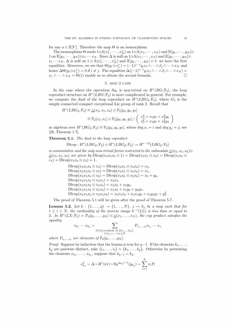
In the case where the operation Sq1 is non-trivial on H∗(BG;F2), the loopcoproduct structure on H∗(LBG;F2) is more complicated in general. For example,we compute the dual of the loop coproduct on H∗(LBG2;F2), where G2 is thesimply-connected compact exceptional Lie group of rank 2. Recall that
H∗(LBG2;F2) ∼= ∧(x3, x5, x6)⊗ F2[y4, y6, y7]
∼= F2[x3, x5]⊗ F2[y4, y6, y7] /
(x43 + x5y7 + x23y6x25 + x3y7 + x23y4
)
as algebras over H∗(BG2;F2) ∼= F2[y4, y6, y7], where deg xi = i and deg yj = j; see[28, Theorem 1.7].
Theorem 5.1. The dual to the loop coproduct
Dlcop : H∗(LBG2;F2)⊗H∗(LBG2;F2)→ H∗−14(LBG2;F2)
is commutative and the only non-trivial forms restricted to the submodule ∧(x3, x5, x6)⊗∧(x3, x5, x6) are given by Dlcop(x3x5x6 ⊗ 1) = Dlcop(x3x5 ⊗ x6) = Dlcop(x3x6 ⊗x5) = Dlcop(x5x6 ⊗ x3) = 1,
Dlcop(x3x5x6 ⊗ x3) = Dlcop(x3x5 ⊗ x3x6) = x3,Dlcop(x3x5x6 ⊗ x5) = Dlcop(x3x5 ⊗ x5x6) = x5,Dlcop(x3x5x6 ⊗ x6) = Dlcop(x3x6 ⊗ x5x6) = x6 + y6,Dlcop(x3x5x6 ⊗ x3x5) = x3x5,Dlcop(x3x5x6 ⊗ x3x6) = x3x6 + x3y6,Dlcop(x3x5x6 ⊗ x5x6) = x5x6 + x5y6 + y4y7,Dlcop(x3x5x6 ⊗ x3x5x6) = x3x5x6 + x3x5y6 + x3y4y7 + y27 .
The proof of Theorem 5.1 will be given after the proof of Theorem 5.7.
Lemma 5.2. Let k : 1, . . . , q → 1, . . . , N, j 7→ kj be a map such that for1 ≤ i ≤ N , the cardinality of the inverse image k−1(i) is less than or equal to2. In H∗(LX ;F2) = F2[y1, . . . , yN ] ⊗ ∧(x1, . . . , xN ), the cup product satisfies theequality
xk1 · · ·xkq=
∑
0≤l≤cardinal of k1,...,kq,1≤i1<···<il≤N
Pi1,...,ilxi1 · · ·xil
where Pi1,...,il are elements of F2[y1, . . . , yN ].
Proof. Suppose by induction that the lemma is true for q−1. If the elements k1, . . . ,kq are pairwise distinct, take i1, . . . , il = k1, . . . , kq. Otherwise by permutingthe elements xk1 , . . . , xkq
, suppose that kq−1 = kq.
x2kq= ∆ H∗(ev) Sq|ykq |−1(ykq
) =
N∑
i=1
xiPi

14 KATSUHIKO KURIBAYASHI AND LUC MENICHI
where P1,. . . ,PN are elements of F2[y1, . . . , yN ]. So
xk1 · · ·xkq=
N∑
i=1
xk1 · · ·xkq−2xiPi.
Since kq = kq−1, by hypothesis, kq /∈ k1, . . . , kq−2. Therefore the cardinal ofk1, . . . , kq−2, i is less or equal to the cardinal of k1, . . . , kq. By our inductionhypothesis,
xk1 · · ·xkq−2xi =∑
0≤l≤cardinal of k1,...,kq−2,i,1≤i1<···<il≤N
Pi1,...,ilxi1 · · ·xil .
Lemma 5.3. Let k : 1, . . . , q + r → 1, . . . , N, j 7→ kj be a non-surjective mapsuch that ∀1 ≤ i ≤ N , the cardinality of the inverse image k−1(i) is ≤ 2. Then
Dlcop(xk1 · · ·xkq⊗ xkq+1 · · ·xkq+r
) = 0.
Proof. We do an induction on r ≥ 0.Case r = 0: By Lemma 5.2, since the cardinal of k1, . . . , kq < N ,
Dlcop(xk1 · · ·xkq⊗ 1) =
∑
0≤l<N,1≤i1<···<il≤N
Dlcop(Pi1,...,ilxi1 · · ·xil ⊗ 1)
where Pi1,...,il are elements of F2[y1, . . . , yN ]. By (3) and (4) of Theorem 3.1, sincel < N ,
Dlcop(Pi1,...,ilxi1 · · ·xil ⊗ 1) = 0.
Suppose now by induction that the Lemma is true for r − 1. Then by (1) ofTheorem 3.1,
Dlcop(xk1 · · ·xkq⊗ xkq+1 · · ·xkq+r
) = xkq+1 Dlcop(xk1 · · ·xkq⊗ xkq+2 · · ·xkq+r
)
+ Dlcop(xk1 · · ·xkq+1 ⊗ xkq+2 · · ·xkq+r)
= xkq+1 ∪ 0 + 0.
Let I = i1, .., il ⊂ 1, ..., N. In ∧(x1, · · · , xN ), denote by xI the generatorxi1 ∪ xi2 ∪ · · · ∪ xil . Since we consider the algebra over F2, the cup product iscommutative, we don’t need to assume that i1 < i2 < · · · < il.
Theorem 5.4. Let I and J be two subsets of 1, . . . , N. Then
Dlcop(xI ⊗ xJ ) =
Dlcop(x1 . . . xN ⊗ xI∩J) if I ∪ J = 1, . . . , N,0 otherwise.
In particular, xI , xJ = ∆(Dlcop(xI⊗xJ )) = ∆(Dlcop(xI∪J⊗xI∩J)) = xI∪J , xI∩J.
Proof. Let i1, .., il denote the elements of the relative complement I−J . Let j1, .., jmdenote the elements of the relative complement J − I. Let k1, .., ku denote theelements of the intersection I ∩ J .
By Lemma 5.3, Dlcop(xi1 . . . xilxk1 . . . xku⊗ xj2 . . . xjmxk1 . . . xku
) = 0. So by(1) of Theorem 3.1,
Dlcop(xi1 . . . xilxk1 . . . xku⊗ xj1 . . . xjmxk1 . . . xku
)
= xj1 ∪ 0 + Dlcop(xi1 . . . xilxj1xk1 . . . xku⊗ xj2 . . . xjmxk1 . . . xku
) .

THE BV ALGEBRA IN STRING TOPOLOGY OF CLASSIFYING SPACES 15
By induction on m, this is equal to
Dlcop(xi1 . . . xilxj1 . . . xjmxk1 . . . xku⊗ xk1 . . . xku
) .
So we have proved that Dlcop(xI ⊗ xJ ) = Dlcop(xI∪J ⊗ xI∩J ). By Lemma 5.3, ifI ∪ J 6= 1, . . . , N then Dlcop(xI ⊗ xJ ) = 0.
Theorem 5.5. Let X be a simply-connected space such that H∗(X ;F2) is the poly-nomial algebra F2[y1, . . . , yN ]. The dual of the loop coproduct admits Dlcop(x1 . . . xN⊗x1 . . . xN ) ∈ Hd(LX ;F2) as unit.
Lemma 5.6. Let a ∈ H∗(LX ;F2)(1) For 1 ≤ i ≤ N , xi ∪Dlcop(a⊗ a) = 0.(2) For any b ∈ H∗(LX ;F2),
Dlcop(Dlcop(a⊗ a)⊗ b) = b ∪Dlcop(Dlcop(a⊗ a)⊗ 1).
Proof. (1) By (1) of Theorem 3.1,
Dlcop(a⊗ axi) = xi Dlcop(a⊗ a) + Dlcop(axi ⊗ a).
Since Dlcop is graded commutative [6], Dlcop(a ⊗ axi) = Dlcop(axi ⊗ a). Soxi Dlcop(a⊗ a) = 0.
(2) By (1) and (1) of Theorem 3.1,
Dlcop(Dlcop(a⊗ a)⊗ bxi) = xi Dlcop(Dlcop(a⊗ a)⊗ b) + 0.
Therefore by induction
Dlcop(Dlcop(a⊗ a)⊗ xi1 . . . xil) = xi1 . . . xil Dlcop(Dlcop(a⊗ a)⊗ 1).
Using (4) of Theorem 3.1, we obtain (2).
Proof of Theorem 5.5. Since Dlcop is graded associative [6] and using (2) of Theo-rem 3.1 twice,
Dlcop(Dlcop(x1 . . . xN ⊗ x1 . . . xN )⊗ 1) = Dlcop(x1 . . . xN ⊗Dlcop(x1 . . . xN ⊗ 1))
= Dlcop(x1 . . . xN ⊗ 1) = 1.
Therefore using (2) of Lemma 5.6,
Dlcop(Dlcop(x1 . . . xN ⊗ x1 . . . xN )⊗ b) = b ∪Dlcop(Dlcop(x1 . . . xN ⊗ x1 . . . xN )⊗ 1)
= b ∪ 1 = b.
The simplest connected Lie group with non-trivial Steenrod operation Sq1 in thecohomology of its classifying space is SO(3).
Theorem 5.7. The cup product and the dual of the loop coproduct on the mod 2free loop cohomology of the classifying space of SO(3) are given by
H∗(LBSO(3);F2) ∼= ∧(x1, x2)⊗ F2[y2, y3]
∼= F2[x1, x2]⊗ F2[y2, y3] /
(x21 + x2
x22 + x2y2 + y3x1
)
as algebras over H∗(BSO(3);F2) ∼= F2[y2, y3], where deg xi = i and deg yj = j.
Dlcop(x1x2 ⊗ 1) = Dlcop(x1 ⊗ x2) = 1,Dlcop(x1x2 ⊗ x1) = x1, Dlcop(x1x2 ⊗ x2) = x2 + y2,Dlcop(x1x2 ⊗ x1x2) = x1x2 + x1y2 + y3,

16 KATSUHIKO KURIBAYASHI AND LUC MENICHI
Proof. The cohomology H∗(BSO(3);F2) is the polynomial algebra on the Stiefel-Whitney classes y2 and y3 of the tautological bundle γ3 ([37, Theorem 7.1] or [38,III.Corollary 5.10]). By Wu formula [38, III.Theorem 5.12(1)], Sq1y2 = y3 andSq2y3 = y2y3. Now the computation of the cup product and of the dual of the loopcoproduct follows from Theorem 3.1.
In the following proof, we detail the computation of the cup product and thedual of the loop coproduct following Theorem 3.1 for a more complicated exampleof Lie group.
Proof of Theorem 5.1. Observe that Sq2y4 = y6, Sq1y6 = y7 [38, VII.Corollary 6.3]
and hence Sq3y4 = Sq1Sq2y4 = y7. From [28, Proof of Theorem 1.7], Sq5y6 = y4y7and Sq6y7 = y6y7. Therefore the computation of the cup product on H∗(LBG2;F2)follows from Theorem 3.1: x23 = x6, x
25 = x3y7 + y4x6 and x26 = x5y7 + y6x6.
Lemma 5.3 implies that monomials with non-trivial loop coproduct are ones onlylisted in the theorem.
By (2) of Theorem 3.1,
Dlcop(x3x5x6⊗1) = Dlcop(x3x5⊗x6) = Dlcop(x3x6⊗x5) = Dlcop(x5x6⊗x3) = 1.
By Lemma 5.3, Dlcop(x3x25 ⊗ 1) = 0. By (1) of Theorem 3.1,
Dlcop(x3x5x6 ⊗ x6) = x6 Dlcop(x3x5x6 ⊗ 1) + Dlcop(x3x5x26 ⊗ 1).
Since x3x5x26 = x3x5(x5y7 + y6x6), by (4) of Theorem 3.1,
Dlcop(x3x5x26 ⊗ 1) = y7 Dlcop(x3x
25 ⊗ 1) + y6 Dlcop(x3x5x6 ⊗ 1) = y7 ∪ 0 + y6 ∪ 1
So finally Dlcop(x3x5x6 ⊗ x6) = x6 + y6.By Theorem 5.4, Dlcop(x3x6 ⊗ x5x6) = Dlcop(x3x5x6 ⊗ x6).Since x3x
25x6 = x5y
27 +x6y6y7+x3x5y7y4+x3x6y6y4, by (1) of Theorem 3.1 and
Lemma 5.3,
Dlcop(x3x5x6 ⊗ x5x6) = x5 Dlcop(x3x5x6 ⊗ x6) + Dlcop(x3x25x6 ⊗ x6)
= x5(x6 + y6) + y27 ∪ 0 + y6y7 ∪ 0 + y7y4 ∪ 1 + y6y4 ∪ 0.
The other computations are left to the reader.
We would like to emphasize that Theorem 5.1 gives at the same time, the cupproduct and the dual of the loop coproduct on H∗(LBG2;F2). As mentioned inIntroduction, if we forget the cup product, then the following Theorem shows thatthe dual of the loop coproduct is really simple:
Theorem 5.8. Let X be a simply-connected space such that H∗(X ;F2) is the poly-nomial algebra F2[V ]. Then with respect to the dual of the loop coproduct, there isan isomorphism of graded algebras between H∗+d(LX ;F2) and the tensor productof algebras H∗(X ;F2)⊗H−∗(ΩX ;F2) ∼= F2[V ]⊗ Λ(sV )∨.Lemma 5.9. Let X be a simply-connected space such that H∗(X ;F2) = F2[V ].Let x1, . . . , xN be a basis of sV .
1) Suppose that i1, .., il∪j1, ..., jm = 1, ..., N. Let k1, .., ku := i1, ..., il∩j1, ..., jm. Then
H∗(ι) Dlcop(xi1 · · ·xil ⊗ xj1 · · ·xjm) = xk1 · · ·xku.

THE BV ALGEBRA IN STRING TOPOLOGY OF CLASSIFYING SPACES 17
2 ) Let Θ : H−∗(ΩX) = ∧(sV )∨∼=→ H∗+d(ΩX) = ∧(sV ) be the linear isomor-
phism defined by
Θ(x∨j1 ∧ · · · ∧ x∨jp) = x1 ∪ · · · ∪ xj1 ∪ · · · ∪ xjp ∪ · · · ∪ xN .
Here ∨ denote the dual and denotes omission. Then the composite Θ−1 H∗(ι) :
H∗+d(LX)→ H∗+d(ΩX)∼=→ H−∗(ΩX) is a morphism of graded algebras preserving
the unit.
Proof of Lemma 5.9. 1) Suppose that |xk1 | ≥ · · · ≥ |xku|. There exists polynomials
P1,. . . ,PN ∈ F2[y1, . . . , yN ] possibly null such that
x2k1= ∆ H∗(ev) Sq|yk1
|−1(yk1) =
N∑
i=1
xiPi.
If Pi is of degree 0, since |xi| > |xk1 |, xi is not one of the elements xk1 ,. . . , xkuand
so by Lemma 5.3, Dlcop(xi1 · · · xk1 · · ·xilxi ⊗ xj1 · · · xk1 · · ·xjm) = 0.If Pi is of degree ≥ 1, by (4) of Theorem 3.1,
H∗(ι) Dlcop(Pixi1 · · · xk1 · · ·xilxi ⊗ xj1 · · · xk1 · · ·xjm) = 0 .
ThereforeH∗(ι)Dlcop(xi1 · · · xk1 · · ·xilx2k1⊗xj1 · · · xk1 · · ·xjm) = 0. Now the same
proof as the proof of Theorem 4.1 shows 1).2) Since H∗(ΩX ;F2) is generated by the xi := σ(yi), 1 ≤ i ≤ N which are
primitives, H∗(ΩX ;F2) is commutative and by [36, 4.20 Proposition], all squaresvanish in H∗(ΩX ;F2). Therefore H∗(ΩX ;F2) is the exterior algebra Λσ(yi)
∨.Let I = i1, .., il ⊂ 1, ..., N. Recall from Theorem 5.4 that in ∧(x1, · · · , xN ),
xI denotes the generator xi1 ∪ xi2 ∪ · · · ∪ xil . Denote also in the exterior alge-bra Λ(x∨1 , · · · , x
∨N ) by x∨I the element x∨i1 ∧ x
∨i2∧ · · · ∧ x∨il . Then with this no-
tation, Θ(x∨I ) = xIc where Ic is the complement of I in 1, ..., N. Let Comp! :
H∗+d(ΩX)⊗H∗+d(ΩX)→ H∗+d(ΩX) be the multiplication defined by Comp!(xI⊗xJ) = xI∩J if I ∪ J = 1, ..., N and 0 otherwise. By (1) and Lemma 5.3,
H∗(ι) : H∗+d(LX) → H∗+d(ΩX) commutes with the products Dlcop and Comp!.Since x(I∪J)c = xIc∩Jc , Θ : H−∗(ΩX) → H∗+d(ΩX) commutes with the exterior
product and Comp!.By Theorem 5.5, Dlcop(x1 . . . xN ⊗ x1 . . . xN ) is the unit of Dlcop. By (1),
Θ−1 H∗(ι) Dlcop(x1 . . . xN ⊗ x1 . . . xN ) = Θ−1(x1 . . . xN ) = 1.
Therefore Θ−1 H∗(ι) preserves also the unit.
Proof of Theorem 5.8. Denote by I := Dlcop(x1 . . . xN ⊗ x1 . . . xN ) the unit ofH∗+d(LX ;F2) (Theorem 5.5). By (7) of Theorem 2.2, the map s! : H∗(X) →H∗+d(LX), a 7→ H∗(ev)(a)I, is a morphism of unital commutative graded alge-bras.
By Lemma 5.3, we have Dlcop(x1 . . . xi . . . xN ⊗ x1 . . . xi . . . xN ) = 0. So letσ : H∗+d(ΩX) → H∗+d(LX) be the unique linear map such that for 1 ≤ i ≤ N ,σ(x1 . . . xi . . . xN ) = x1 . . . xi . . . xN and such that σ Θ : H−∗(ΩX) = Λ(sV )∨ →H∗+d(LX) is a morphism of unital commutative graded algebras. For 1 ≤ i ≤ N ,Θ−1 H∗(ι) σ Θ(x∨i ) = x∨i . By Lemma 5.9, the composite Θ−1 H∗(ι) :
H∗+d(LX) → H∗+d(ΩX)∼=→ H−∗(ΩX) is a morphism of graded algebras. So the
composite Θ−1 H∗(ι)σ Θ is the identity map and σ is a section of H∗(ι). So by

18 KATSUHIKO KURIBAYASHI AND LUC MENICHI
Leray-Hirsch theorem, the linear morphism ofH∗(X)-modulesH∗(X)⊗H∗(ΩX)→H∗(LX), a⊗ g 7→ H∗(ev)(a)σ(g), is an isomorphism.
The composite
ϕ : H∗(X)⊗H−∗(ΩX)s!⊗σΘ→ H∗+d(LX)⊗H∗+d(LX)
Dlcop→ H∗+d(LX)
is a morphism of commutative graded algebras with respect to the dual of the loopcoproduct. By (4) of Theorem 3.1 and since I is the unit for Dlcop, ϕ(a ⊗ g) =Dlcop(H∗(ev)(a)I⊗σ Θ(g)) = H∗(ev)(a)σ Θ(g). Therefore ϕ is an isomorphism.
Example 5.10. With respect to the dual of the loop coproduct, there is an isomor-phism of algebras between H∗+3(LBSO(3);F2) and
H−∗(SO(3);F2)⊗H∗(BSO(3);F2) ∼= ∧(u−1, u−2)⊗ F2[v2, v3].
Proof. By Theorem 5.5, Dlcop(x1x2 ⊗ x1x2) = x1x2 + x1y2 + y3 is the unit for thedual of the loop coproduct on H∗+3(LBSO(3);F2). By Lemma 5.3,
Dlcop(x1 ⊗ x1) = Dlcop(x2 ⊗ x2) = 0.
So let ϕ : ∧(u−1, u−2)⊗ F2[v2, v3]→ H∗+3(LBSO(3);F2) be the unique morphismof algebras such that ϕ(u−2) = x1, ϕ(u−1) = x2, ϕ(v2) = y2(x1x2 + x1y2 + y3) andϕ(v3) = y3(x1x2 + x1y2 + y3).
For all i, j ≥ 0, we see that ϕ(vi2vj3) = yi2y
j3(x1x2 +x1y2 + y3), ϕ(u−1u−2v
i2v
j3) =
yi2yj3, ϕ(u−1v
i2v
j3) = x2y
i2y
j3 and ϕ(u−2v
i2v
j3) = x1y
i2y
j3. Therefore ϕ sends a linear
basis of ∧(u−1, u−2) ⊗ F2[v2, v3] to a linear basis H∗+3(LBSO(3);F2). So ϕ is anisomorphism.
Example 5.11. With respect to the dual of the loop coproduct, there is an isomor-phism of algebras between H∗+14(LBG2;F2) and H−∗(G2;F2) ⊗ H
∗(BG2;F2) ∼=∧(u−3, u−5, u−6)⊗ F2[v4, v6, v7].
Proof. By Theorem 5.5, Dlcop(x3x5x6 ⊗ x3x5x6) = x3x5x6 + x3x5y6 + x3y4y7 + y27is the unit for the dual of the loop coproduct on H∗+14(LBG2;F2). By Lemma 5.3,
Dlcop(x5x6 ⊗ x5x6) = Dlcop(x3x6 ⊗ x3x6) = Dlcop(x3x5 ⊗ x3x5) = 0.
So let ϕ : ∧(u−3, u−5, u−6)⊗ F2[v4, v6, v7]→ H∗+14(LBG2;F2) be the unique mor-phism of algebras such that ϕ(u−3) = x5x6, ϕ(u−5) = x3x6, ϕ(u−6) = x3x5,ϕ(v4) = y4(x3x5x6+x3x5y6+x3y4y7+y
27), ϕ(v6) = y6(x3x5x6+x3x5y6+x3y4y7+y
27)
and ϕ(v7) = y7(x3x5x6 + x3x5y6 + x3y4y7 + y27).
For all i, j and k ≥ 0, we see that ϕ(vi4vj6v
k7 ) = yi4y
j6y
k7 (x3x5x6 + x3x5y6 +
x3y4y7 + y27), ϕ(u−3u−5u−6vi4v
j6v
k7 ) = yi4y
j6y
k7 , ϕ(u−3u−5v
i4v
j6v
k7 ) = (x6 + y6)y
i4y
j6y
k7 ,
ϕ(u−3u−6vi4v
j6v
k7 ) = x5y
i4y
j6y
k7 , ϕ(u−5u−6v
i4v
j6v
k7 ) = x3y
i4y
j6y
k7 , ϕ(u−3v
i4v
j6v
k7 ) =
x5x6yi4y
j6y
k7 , ϕ(u−5v
i4v
j6v
k7 ) = x3x6y
i4y
j6y
k7 and ϕ(u−6v
i4v
j6v
k7 ) = x3x5y
i4y
j6y
k7 . There-
fore ϕ sends a linear basis of ∧(u−3, u−5, u−6) ⊗ F2[v4, v6, v7] to a linear basisH∗+14(LBG2;F2). So ϕ is an isomorphism.
Lemma 5.12. Let (A,⊙) be a commutative unital associative graded algebra. Letx ∈ A such that x ⊙ x = 1. Let ψ : A → A be the linear morphism mappinga to x ⊙ a. Then ψ is an involutive isomorphism such that for any a, b in A,ψ(a)⊙ ψ(b) = a⊙ b.
Proof. ψ(a)⊙ψ(b) = (x⊙ a)⊙ (x⊙ b) = (x⊙ x)⊙ (a⊙ b) = 1⊙ (a⊙ b) = a⊙ b.

THE BV ALGEBRA IN STRING TOPOLOGY OF CLASSIFYING SPACES 19
Second proof of Theorem 5.8 which gives another (better?) algebra isomorphism. Bycommutativity and associativity of Dlcop and Theorem 5.5, applying Lemma 5.12,ψ : H∗(X)⊗H∗+d(ΩX)→ H∗+d(LX) defined by
ψ(a⊗ xk1 . . . xku) = Dlcop(x1 . . . xN ⊗ axk1 . . . xku
)
is an involutive isomorphism such that
Dlcop(ψ(a⊗ xI)⊗ ψ(b⊗ xJ )) = Dlcop(axI ⊗ bxJ)
for any subsets I and J of 1, ..., N.Case I ∪ J = 1, ..., N. By Theorem 5.4,
Dlcop(axI⊗bxJ) = Dlcop(x1 . . . xN⊗abxI∩J) = ψ(ab⊗xI∩J) = ψ(ab⊗Comp!(xI⊗xJ)).
Case I∪J 6= 1, ..., N. By Theorem 5.4, Dlcop(axI⊗bxJ) = 0 and Comp!(xI ⊗xJ) = 0.
Therefore ψ is a morphism of graded algebras.One can show that ψ(1⊗Θ(x∨i )), ψ(1⊗Θ(x∨j )) = 0. That is why this isomor-
phism might be better.
Theorem 5.13. As a Batalin-Vilkovisky algebra,
H∗+3(LBSO(3);F2) ∼= ∧(u−1, u−2)⊗ F2[v2, v3]
where for all i, j ≥ 0, ∆(vi2vj3) = 0, ∆(u−1u−2v
i2v
j3) = iu−2v
i−12 vj3 + ju−1v
i2v
j−13 ,
∆(u−2vi2v
j3) = iu−1v
i−12 vj3 + jvi2v
j−13 + ju−2v
i+12 vj−1
3 + ju−1u−2vi2v
j3 and
∆(u−1vi2v
j3) = ivi−1
2 vj3 + (i+ j)u−2vi2v
j3 + iu−1u−2v
i−12 vj+1
3 + ju−1vi+12 vj−1
3 .
In particular 1 /∈ Im ∆.
Proof. Theorem 5.7 gives the BV-algebra H∗+3(LBSO(3);F2) since ∆ is a deriva-tion with respect to the cup product. In the proof of Example 5.10, the isomorphismof algebras ϕ : ∧(u−1, u−2) ⊗ F2[v2, v3] → H∗+3(LBSO(3);F2) of Theorem 5.8 ismade explicit on generators. We now transport the operator ∆ using ϕ.
In degree 1, the ∆ operator is given by ∆(u−1u−2v22) = 0 and
∆(u−2v3) = ∆(u−1v2) = 1 + u−2v2 + u−1u−2v3.
Theorem 5.14. As a Batalin-Vilkovisky algebra,
H∗+14(LBG2;F2) ∼= ∧(u−3, u−5, u−6)⊗ F2[v4, v6, v7]
where for all i, j, k ≥ 0, ∆(vi4vj6v
k7 ) = 0,
∆(u−3u−5u−6vi4v
j6v
k7 ) = iu−5u−6v
i−14 vj6v
k7 + ju−3u−6v
i4v
j−16 vk7
+ ku−3u−5vi4v
j6v
k−17 + ku−3u−5u−6v
i4v
j+16 vk−1
7 ,
∆(u−5u−6vi4v
j6v
k7 ) = iu−3u−5v
i−14 vj6v
k7 + iu−3u−5u−6v
i−14 vj+1
6 vk7
+ ju−6vi4v
j−16 vk7 + ku−5v
i4v
j6v
k−17 ,
∆(u−3u−6vi4v
j6v
k7 ) = iu−6v
i−14 vj6v
k7 + ju−5u−6v
i4v
j−16 vk+1
7
+ ju−3u−5vi+14 vj−1
6 vk7 + ju−3u−5u−6vi+14 vj6v
k7 + ku−3v
i4v
j6v
k−17 ,

20 KATSUHIKO KURIBAYASHI AND LUC MENICHI
∆(u−3u−5vi4v
j6v
k7 ) = iu−5v
i−14 vj6v
k7 + iu−5u−6v
i−14 vj+1
6 vk7
+ ju−3vi4v
j−16 vk7 + (j + 1 + k)u−3u−6v
i4v
j6v
k7
∆(u−6vi4v
j6v
k7 ) = iu−3v
i−14 vj6v
k7 + ju−5v
i+14 vj−1
6 vk7 + ju−3u−5vi4v
j−16 vk+1
7
+(j+k)u−3u−5u−6vi4v
j6v
k+17 +kvi4v
j6v
k−17 +ku−6v
i4v
j+16 vk−1
7 +ku−5u−6vi+14 vj6v
k7 ,
∆(u−3vi4v
j6v
k7 ) = ivi−1
4 vj6vk7 + iu−6v
i−14 vj+1
6 vk7 + (i+ k)u−5u−6vi4v
j6v
k+17
+ iu−3u−5u−6vi−14 vj6v
k+27 + ju−5v
i4v
j−16 vk+1
7 + ju−3u−6vi+14 vj−1
6 vk+17
+(j+ k)u−3u−5vi+14 vj6v
k7 +(j+ k)u−3u−5u−6v
i+14 vj+1
6 vk7 + ku−3vi4v
j+16 vk−1
7 and
∆(u−5vi4v
j6v
k7 ) = iu−3u−5v
i−14 vj+1
6 vk7 + iu−3u−5u−6vi−14 vj+2
6 vk7 + jvi4vj−16 vk7
+(j+k)u−6vi4v
j6v
k7+ju−5u−6v
i+14 vj−1
6 vk+17 +ju−3u−5u−6v
i4v
j−16 vk+2
7 +ku−5vi4v
j+16 vk−1
7 .
In particular 1 /∈ Im ∆.
Proof. Theorem 5.1 gives the BV-algebra H∗+14(LBG2;F2) since ∆ is a derivationwith respect to the cup product. In the proof of Example 5.11, the isomorphism ofalgebras ϕ : ∧(u−3, u−5, u−6) ⊗ F2[v4, v6, v7] → H∗+14(LG2;F2) of Theorem 5.8 ismade explicit on generators. We now transport the operator ∆ using ϕ.
In degree 1, the ∆ operator is given by ∆(u−5u−6v26) = 0,
∆(u−3u−5u−6v24v7) = ∆(u−5u−6v
34) = u−3u−5v
24 + u−3u−5u−6v
24v6,
∆(u−3u−6v4v6) = u−6v6 + u−5u−6v4v7 + u−3u−5v24 + u−3u−5u−6v
24v6 and
∆(u−6v7) = ∆(u−5v6) = ∆(u−3v4) = 1 + u−6v6 + u−5u−6v4v7 + u−3u−5u−6v27 .
Note that ϕ−1 ∆ ϕ(yi ⊗ x∨i ) = ϕ−1(x1 . . . xN ) is independent of i.
6. Relation with Hochschild cohomology
Let K be any field. Let G be a connected compact Lie group of dimension d.
Conjecture 6.1. [6, Conjecture 68] There is an isomorphism of Gerstenhaberalgebras
H∗+d(LBG)∼=→ HH∗(S∗(G), S∗(G)).
Suppose that H∗(BG;K) is a polynomial algebra K[V ] = K[y1, . . . , yN ]. It fol-lows from [40, Theorem 9, p. 572] (See also [31, Proposition 8.21]) that BG isK-formal. Then BG is K-coformal and H∗(G;K) is the exterior algebra ∧(sV )∨.Indeed, since BG is K-formal, the Cobar construction ΩH∗(BG) is weakly equiva-lent as algebras to S∗(G). Let Ai denote the exterior algebra Λs−1(y∨i ). Then EZ,the Eilenberg-Zilber map and ε, the counit of the adjunction between the Bar andthe Cobar construction give the quasi-isomorphims of algebras
ΩH∗(BG) = Ω(⊗Ni=1BAi) ⊗N
i=1ΩBAi≃
EZoo≃
⊗Ni=1εi //⊗N
i=1Ai = Λs−1V ∨.
Alternatively, since BG is K-formal, we can use the implication (2) ⇒ (1) in [2,Theorem 2.14].

THE BV ALGEBRA IN STRING TOPOLOGY OF CLASSIFYING SPACES 21
Therefore, we have the isomorphism of Gerstenhaber algebras
HH∗(S∗(G), S∗(G)) ∼= HH∗(H∗(G;K), H∗(G;K)) ∼= HH∗(∧(sV )∨,∧(sV )∨).
By Theorem F.3 i) and ii) as graded algebras,
HH∗(∧(sV )∨,∧(sV )∨) ∼= ∧(sV )∨ ⊗K[V ] ∼= H−∗(G;K)⊗H∗(BG;K).
So in Theorem 5.8, we have checked Conjecture 6.1 only for the algebra structurewhen K = F2. When K = F2, we would like to check conjecture 6.1 also for theGerstenhaber algebra structure.
The following theorem shows that the conjecture is true for the Gerstenhaberalgebra structure when K is a field of characteristic different from 2.
Theorem 6.2. Under the hypothesis (H), the free loop space cohomology of theclassifying space of G, H∗+dimG(LBG;K) is isomorphic as Batalin-Vilkovisky al-gebra to the Hochschild cohomology of H∗(G;K), HH∗(H∗(G;K);H∗(G;K)). Inparticular the underlying Gerstenhaber algebras are isomorphic.
Proof. By hypothesis, H∗(BG) ∼= K[V ] = K[yi] as algebras. Then H∗(G) ∼=Λ(sV )∨ = Λx∨j as algebras.
Let Ψ : sV → (sV )∨∨ be the canonical isomorphism of the graded vector spacesV into its bidual. By definition, Ψ(sv)(ϕ) = (−1)|ϕ||sv|ϕ(sv) for any linear formϕ on sV .
By Theorem F.3 iii), we have the BV-algebra isomorphismHH∗(H∗(G);H∗(G)) ∼=Λ(sV )∨ ⊗K[s−1(sV )∨∨] where for any v ∈ V and ϕ ∈ (sV )∨,
∆((1⊗s−1Ψ(sv))(ϕ⊗1)) = (−1)|v|s−1Ψ(sv), ϕ = −Ψ(sv)(ϕ) = −(−1)|ϕ||sv|ϕ(sv)
and where ∆ is trivial on Λ(sV )∨ and on K[s−1(sV )∨∨].The isomorphism of algebras Id ⊗ K[s−1Ψ] : Λ(sV )∨ ⊗ K[V ] → Λ(sV )∨ ⊗
K[s−1(sV )∨∨] is a isomorphism of BV-algebras if for any v ∈ V and ϕ ∈ (sV )∨,∆((1⊗ v)(ϕ ⊗ 1)) = −(−1)|ϕ||sv|ϕ(sv) and if ∆ is trivial on Λ(sV )∨ and on K[V ].
Taking v = yi and ϕ = σ(yj)∨ = x∨j , we obtained that ∆(yi ⊗ x
∨j ) = 1 if i = j
and 0 otherwise like in Theorem 4.3.
Theorem 6.3. For G = SO(3) or G = G2, the free loop space modulo 2 cohomol-ogy of the classifying space of G, H∗+dimG(LBG;F2) is not isomorphic as Batalin-Vilkovisky algebras to the Hochschild cohomology of H∗(G;F2), HH
∗(H∗(G;F2);H∗(G;F2))although when G = SO(3) the underlying Gerstenhaber algebras are isomorphic.
The main result of [34] is that the same phenomenon appears for Chas-Sullivanstring topology even in the simple case of the two dimensional sphere S2.
Definition 6.4. Let A be an augmented graded algebra. Let F 0(A) := A andFn(A) := A · A · · · · A for n ≥ 1 be the augmentation filtration [36, 7.1]. We saythat A is Hausdorff [31, Lemma 3.10] if ∩n∈NF
n(A) = 0.
Lemma 6.5. Let A and B be a morphism of graded algebras between two Hausdorffaugmented graded algebras such that the only indecomposables elements of A andB, Q(A) and Q(B), are the zero vectors. Let f : A → B be a morphism ofgraded algebras. Then f preserves the augmentations. Let d ∈ N be a non-negativeinteger. Suppose moreover that B = B≥−d, i.e. B is concentrated in degrees greateror equal than −d and that B is graded commutative. Then f is surjective iff Q(f)is surjective.

22 KATSUHIKO KURIBAYASHI AND LUC MENICHI
Proof. When d = 0, A0 = 0 and B0 = 0, this Lemma is Proposition 3.8 of [36].But the proof of [36] cannot be easily generalized. Therefore we provide a proof.
Denote by Q : A։ Q(A) := A
A·Athe quotient map. The sequence
⊕ni=1
(A
⊗i−1⊗A · A⊗A
⊗n−i)→ A
⊗n Q⊗n
։ Q(A)⊗n → 0
is exact. Alternatively, since over a field K, A = A ·A⊕Q(A),
0→ +ni=1
(A
⊗i−1⊗A ·A⊗A
⊗n−i)→ A
⊗n Q⊗n
։ Q(A)⊗n → 0
is a short exact sequence. Therefore the iterated multiplication of A induces anatural map Q(A)⊗n
։ Fn(A)/Fn+1(A) obviously surjective.Let x ∈ A = F 1(A) with x 6= 0. Since ∩n∈NF
n(A) = 0, there exists r ≥ 1such that x ∈ F r(A) and x /∈ F r+1(A). Therefore x is the product of r elementsof A, x1 . . . xr such that Q(x1) ⊗ · · · ⊗ Q(xr) 6= 0. By hypothesis, Q(A)0 = 0.So the xi’s and the f(xi)’s are of degree different from 0. So f(xi) ∈ B. Andf(x) = Πif(xi) ∈ B: we have proved that f preserves the augmentations.
Let y ∈ Fn(B) with y 6= 0. Similarly, y is the product of r ≥ n elements of B,y1 . . . yr such that all the Q(yi) ’s are non zero. Since Q(B)0 = 0, the yi’s areall of degree different from 0. Since B is graded commutative, B<−d = 0 andy 6= 0, there is at most d elements yi’s of negative degree in the product y1 . . . yr.So there is at least r − d elements yi’s of positive degree. Therefore the degree ofy is at least d × (−1) + (r − d) × 1: we have proved that the non-zero elements ofFn(B) are all of degree greater than or equal to n− 2d.
Assume that Q(f) is surjective. Then Q(f)⊗n : Q(A)⊗n։ Q(B)⊗n is also
surjective. Since the following square is commutative by naturality,
Q(A)⊗n
Q(f)⊗n
// Fn(A)/Fn+1(A)
Grnf
Q(B)⊗n // Fn(B)/Fn+1(B),
the map induced by f , Grnf , is also surjective. In a fixed degree, consider thecommutative diagram
0 // Fn+1(A) //
f |Fn+1(A)
Fn(A) //
f |Fn(A)
Fn(A)/Fn+1(A)
Grnf
// 0
0 // Fn+1(B) // Fn(B) // Fn(B)/Fn+1(B) // 0
with exact rows. Suppose by induction that the restriction of f to Fn+1(A),f |Fn+1(A), is surjective. Then by the five Lemma, f |Fn(A), is also surjective.Since Fn(B) is concentrated in degrees greator than or equal to n− 2d, in a fixeddegree, for large n, Fn(B) is trivial and we can start the induction. Thereforef = f |F 0(A) is surjective.
Proof of Theorem 6.3. Since H∗(G) is an exterior algebra, by Example F.2 b),1 ∈ Im ∆ in the BV-algebra HH∗(H∗(G);H∗(G)). On the contrary, by Theo-rems 5.13 and 5.14, the unit 1 does not belong to the image of ∆ in the BV-algebra
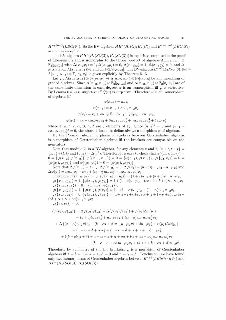
THE BV ALGEBRA IN STRING TOPOLOGY OF CLASSIFYING SPACES 23
H∗+dimG(LBG;F2). So the BV-algebrasHH∗(H∗(G);H∗(G)) andH
∗+dimG(LBG;F2)are not isomorphic.
The BV-algebraHH∗(H∗(SO(3)), H∗(SO(3))) is explicitly computed in the proofof Theorem 6.2 and is isomorphic to the tensor product of algebras Λ(x−2, x−1)⊗F2[y2, y3] with ∆(x−2y3) = 1, ∆(x−2y2) = 0, ∆(x−1y2) = 1, ∆(x−1y3) = 0, and ∆is trivial on Λ(x−2, x−1)⊗1 and on 1⊗F2[y2, y3]. The BV-algebraH
∗+3(LBSO(3);F2) ∼=Λ(u−2, u−1)⊗ F2[v2, v3] is given explicitly by Theorem 5.13.
Let ϕ : Λ(x−2, x−1)⊗ F2[y2, y3] → Λ(u−2, u−1)⊗ F2[v2, v3] be any morphism ofgraded algebras. Since Λ(x−2, x−1)⊗ F2[y2, y3] and Λ(u−2, u−1)⊗ F2[v2, v3] are ofthe same finite dimension in each degree, ϕ is an isomorphism iff ϕ is surjective.By Lemma 6.5, ϕ is surjective iff Q(ϕ) is surjective. Therefore ϕ is an isomorphismof algebras iff
ϕ(x−2) = u−2,
ϕ(x−1) = u−1 + εu−1u−2v2,
ϕ(y2) = v2 + au−2v22 + bu−1u−2v2v3 + cu−1v3,
ϕ(y3) = v3 + αu−2v2v3 + βu−1u−2v23 + γu−1u−2v
32 + δu−1v
22
where ε, a, b, c, α, β, γ, δ are 8 elements of F2. Since (u−2)2 = 0 and (u−1 +
εu−1u−2v2)2 = 0, the above 4 formulas define always a morphism ϕ of algebras.
By the Poisson rule, a morphism of algebras between Gerstenhaber algebrasis a morphism of Gerstenhaber algebras iff the brackets are compatible on thegenerators.
Note that modulo 2, in a BV-algebra, for any elements z and t, z + t, z + t =z, z+t, t and z, z = ∆(z2). Therefore it is easy to check that ϕ(x−2, x−2) =0 = ϕ(x−2), ϕ(x−2), ϕ(x−1, x−1) = 0 = ϕ(x−1), ϕ(x−1), ϕ(y2, y2) = 0 =ϕ(y2), ϕ(y2) and ϕ(y3, y3) = 0 = ϕ(y3), ϕ(y3).
Note that ∆ϕ(x−1) = εu−2, ∆ϕ(x−2) = 0, ∆ϕ(y2) = (b+c)(u−2v3+u−1v2) and∆ϕ(y3) = αu−1v3 + αv2 + (α+ γ)u−2v
22 + αu−1u−2v2v3.
Therefore ϕ(x−2, y2) = 0, ϕ(x−2), ϕ(y2) = (1 + c)u−1 + (b + c)u−1u−2v2,ϕ(x−1, y2) = 1, ϕ(x−1), ϕ(y2) = 1+(1+ ε)u−2v2+(εc+1+ b+ c)u−1u−2v3,ϕ(x−2, x−1) = 0 = ϕ(x−2), ϕ(x−1),ϕ(x−2, y3) = 1, ϕ(x−2), ϕ(y3) = 1 + (1 + α)u−2v2 + (1 + α)u−1u−2v3,ϕ(x−1, y3) = 0, ϕ(x−1), ϕ(y3) = (1+α+ε+α)u−1v2+(ε+1+α+ε)u−2v3+
(εδ + α+ γ + εα)u−1u−2v22 ,
ϕ(y2, y3) = 0,
ϕ(y2), ϕ(y3) = ∆ϕ(y2)ϕ(y3) + ∆(ϕ(y2)ϕ(y3)) + ϕ(y2)∆ϕ(y3)
= (b+ c)(u−2v23 + u−1v2v3 + (α+ δ)u−1u−2v
22v3)
+ ∆((a+ α)u−2v
22v3 + (b+ cα+ β)u−1u−2v2v
23 + δu−1v
32
)+ ϕ(y2)∆ϕ(y3)
= (a+ α+ δ + α)v22 + (a+ α+ δ + α+ γ + aα)u−2v32
+ ((b + c)(α+ δ) + a+ α+ δ + α+ aα+ bα+ cα+ cγ)u−1u−2v22v3
+ (b + c+ α+ cα)u−1v2v3 + (b+ c+ b+ cα+ β)u−2v23 .
Therefore, by symmetry of the Lie brackets, ϕ is a morphism of Gerstenhaberalgebras iff ε = b = c = α = 1, β = 0 and a = γ = δ. Conclusion: we have foundonly two isomorphisms of Gerstenhaber algebras between H∗+3(LBSO(3);F2) andHH∗(H∗(SO(3)), H∗(SO(3))).

24 KATSUHIKO KURIBAYASHI AND LUC MENICHI
7. Triviality of the loop product when H∗(BG) is polynomial
This section is independent of the rest of the paper. Recall the dual of the loopcoproduct introduced by Sullivan for manifolds H∗(LM)⊗H∗(LM)→ H∗+d(LM)is (almost) trivial [44]. In this section, we prove that the loop product for classifyingspaces of Lie groups H∗(LBG)⊗H∗(LBG)→ H∗+d(LBG) is trivial if the inclusionof the fibre in cohomology H∗(j) : H∗(LBG;K) ։ H∗(G;K) is surjective (Theo-rem 7.1). We also explain that this condition H∗(j) : H∗(LBG;K) ։ H∗(G;K)surjective is equivalent to our hypothesis H∗(BG) polynomial (Theorem 7.3).
Theorem 7.1. Let BG be the classifying space of a connected Lie group G. Supposethat the map induced in cohomology H∗(LBG;K) ։ H∗(G;K) is surjective. Thenthe loop product on H∗(LBG;K) is trivial while the loop coproduct is injective.
This result is a generalization of [12, Theorem D] in which it is assumed that theunderlying field is of characteristic zero. If CharK 6= 2, the triviality of the loopproduct was first proved by Tamanoi [43, Theorem 4.7 (2)]. The second authorand David Chataur conjecture that the loop coproduct on H∗(LBG) has always acounit. Assuming that the loop coproduct on H∗(LBG) has a counit, obviouslythe loop coproduct is injective and it follows from [43, Theorem 4.5 (i)] that theloop product on H∗(LBG) is trivial.
The injectivity described in Theorem 7.1 follows from a consideration of theEilenberg-Moore spectral sequences associated with appropriate pullback diagrams.In fact, the induced maps Comp! and H(q) in the cohomology are epimorphisms;see Proposition 7.2.
Let ΩXι→ LX ։ X be the free loop fibration. The following proposition is a
key to proving Theorem 7.1.
Proposition 7.2. Let X be a simply-connected space. Suppose that H∗(ι) : H∗(LX)→H∗(ΩX) induced by the inclusion is surjective. Then one has(1) the map H∗(q) induced by the inclusion q : LX ×X LX → LX × LX is anepimorphism.(2) Suppose moreover that X is the classifying space of a connected Lie group G.
Then, for the map Comp : LBG×BG LBG→ LBG, Comp! is an epimorphism.
Proof of Theorem 7.1. By Proposition 7.2 (1) and (2), we see that the dual to the
loop coproduct Dlcop := Comp! H∗(q) on H∗(LBG) is surjective. Since q! isH∗(LBG×LBG)-linear and decreases the degrees, q! H∗(q) = 0. By Proposition7.2 (1), H∗(q) is an epimorphism. Therefore q! is trivial and the dual of the loopproduct Dlp := q! H∗(Comp) on H∗(LBG) is also trivial.
Proof of Proposition 7.2. Consider the two Eilenberg-Moore spectral sequences as-sociated to the free loop fibration mentioned above and to the pull-back diagram
LX ×X LXq //
ev
LX × LX
ev×ev
X
δ // X ×X

THE BV ALGEBRA IN STRING TOPOLOGY OF CLASSIFYING SPACES 25
SinceH∗(LX) is a freeH∗(X)-module by Leray-Hirsch theorem, these two Eilenberg-Moore spectral sequences are concentrated on the 0-th column. So the two mor-phisms of graded algebras
H∗(ι) ⊗H∗(X) η : H∗(LX)⊗H∗(X) K∼=→ H∗(ΩX)
and
H∗(q)⊗H∗(X)⊗2H∗(ev) : (H∗(LX)⊗H∗(LX))⊗H∗(X)⊗2H∗(X)∼=→ H∗(LX×XLX)
are isomorphisms. In particular, H∗(q) is an epimorphism and we have an isomor-phism of graded vector spaces between H∗(LX ×X LX) and H∗(LX)⊗H∗(ΩX).
Consider the Leray-Serre spectral sequence E∗,∗r , dr of the homotopy fibration
ΩX→LX ×X LXComp→ LX . Since H∗(LX ×X LX) is isomorphic to H∗(LX) ⊗
H∗(ΩX), by [38, III.Lemma 4.5 (2)], E∗,∗r , dr collapses at the E2-term. Then
for X = BG, the integration along the fibre Comp! : H∗(LBG ×BG LBG) →H∗−dimG(LBG) is surjective.
Let G be a connected Lie group and K a field of arbitrary characteristic. Let
F : Gj→ LBG→ BG be the free loop fibration.
Theorem 7.3. The induced map H∗(j) : H∗(LBG;K) → H∗(G;K) is surjectiveif and only if H∗(BG;K) is a polynomial algebra.
Proof. The ”if” part follows from the usual EMSS argument. In fact, suppose thatH∗(BG;K) ∼= K[V ]. Then the EMSS for the universal bundle F ′ : G→ EG→ BGallows one to deduce that H∗(G;K) ∼= ∧(sV ). By using the EMSS for the fibresquare ([26, Proof of Theorem 1.2] or [28, Proof of Theorem 1.6])
LBG //
BGI
BG
δ// BG×BG,
we see that H∗(LBG;K) ∼= H∗(BG;K) ⊗ ∧(sV ) as an H∗(BG) = K[V ]-algebra.This implies that the Leray-Serre spectral sequence (LSSS) for F collapses at theE2-term and hence H∗(j) is surjective. See the beginning of section 3 for an alter-native proof which uses module derivations.
Suppose that H∗(j) is surjective. We further assume that CharK = 2. By theargument in [28, Remark 1.4] or [21, Proof of Theorem 2.2], we see that the Hopfalgebra A = H∗(G;K) is cocommutative and so primitively generated; that is, thenatural map P (A) → Q(A) is surjective. By [28, Lemma 4.3], this yields thatH∗(G;K) ∼= ∧(x1, ..., xN ), where xi is primitive for any 1 ≤ i ≤ N . The sameargument as in the proof of [38, Chapter 7, Theorem 2.26(2)] allows us to deducethat each xi is transgressive in the LSSS Er, dr for F
′. To see this more precisely,we recall that the action of G on EG gives rise to a morphism of spectral sequence
µ∗r : Er, dr → Er ⊗H
∗(G;K), dr ⊗ 1
for which µ∗2 = 1 ⊗ µ∗ : H∗(BG;K) ⊗ H∗(G;K) → H∗(BG;K) ⊗ H∗(G;K) ⊗
H∗(G;K), where µ : G×G→ G denotes the multiplication on G; see [38, Chapter7, Section 2].

26 KATSUHIKO KURIBAYASHI AND LUC MENICHI
Suppose that there exists an integer i such that xj is transgressive for j < i butnot xi. Then we see that for some r < deg xi + 1, dr(xi) 6= 0 and dp(xi) = 0 ifp < r. We write
dr(xi) =∑
l
bl ⊗ xl1 · · ·xlsl ,
where each bl is a non-zero element of H∗(BG;K) and 1 ≤ lu ≤ N for any l and u.The equality µ∗
rdr(xi) = (dr ⊗ 1)µ∗r(xi) implies that
∑
l
bl ⊗ xl1 · · ·xlsl−1 ⊗ xlsl + · · · = dr ⊗ 1(1⊗ xi ⊗ 1 + 1⊗ 1⊗ xi)
=∑
l
bl ⊗ xl1 · · ·xlsl ⊗ 1,
which is a contradiction. Observe that xi and xlu are primitive. Thus it followsthat xi is transgressive for any 1 ≤ i ≤ N .
In the case where CharK = p 6= 2, since H∗(j) is surjective by assumption,it follows from the argument in [28, Remark 1.4] that H∗(G;Z) has no p-torsion.Observe that to obtain the result, the connectedness of the loop space is assumed.By virtue of [38, Chapter 7, Theorem 2.12], we see that H∗(BG;K) is a polynomialalgebra. This completes the proof.
The following theorem give another characterisation of our hypothesis thatH∗(BG)is polynomial.
Theorem 7.4. Let G be a connected Lie group. Then the following three conditionsare equivalent:
1) H∗(BG;K) is a polynomial algebra on even degree generators.2) BG is K-formal and H∗(BG;K) is strictly commutative.3) The singular cochain algebra S∗(BG;K) is weakly equivalent as algebras to a
strictly commutative differential graded algebra A.
Strictly commutative means that a2 = 0 if a ∈ Aodd (K can be a field of charac-teristics two). We conjecture that over a field of characteristics two, this Theoremremains valid if we omit ”on even degree generators” in 1), ”and H∗(BG;K) isstrictly commutative” in 2) and ”strictly” in 3).
Proof. 1 ⇒ 2. Suppose that H∗(BG;K) is a polynomial algebra. Then by thebeginning of section 6, BG is K-formal.
2⇒ 3. Formality means that we can take A = (H∗(BG;K), 0) in 3).3⇒ 1. Let Y be a simply connected space such that S∗(Y ;K) is weakly equiva-
lent as algebras to a strictly commutative differential graded algebra A. Let (ΛV, d)be a minimal Sullivan model of A. Consider the semifree-(ΛV, d) resolution of (K, 0),(ΛV ⊗ ΓsV,D) given in [16, Proposition 2.4] or [33, Lemma 7.2]. Then the tensorproduct of commutative differential graded algebras (K, 0)⊗(ΛV,d) (ΛV ⊗ΓsV,D) ∼=
(ΓsV,D) has a trivial differential D = 0 [16, Corollary 2.6]. Therefore we have theisomorphisms of graded vector spaces
H∗(ΩY ) ∼= TorS∗(Y ;K)(K,K) ∼= Tor(ΛV,d)(K,K) ∼= H∗(ΓsV,D) ∼= ΓsV.
IfH∗(ΩY ) is of finite dimension then the suspension of V , sV , must be concentratedin odd degree and so V must be in even degree and d = 0, thus Y is K-formal andH∗(Y ) is polynomial in even degree.

THE BV ALGEBRA IN STRING TOPOLOGY OF CLASSIFYING SPACES 27
Appendix A. Review of [6] with signs corrections
In this appendix, we review the results of Chataur and the second author in [6].And we correct a sign mistake.Integration along the fibre in homology with corrected sign. Let F →
Eproj→ B be an oriented fibration with B path-connected; that is, the homology
H∗(F ;K) is concentrated in degree less than or equal to n, π1(B) acts on Hn(F ;K)trivially and Hn(F ;K) ∼= K. In what follows, we write H∗(X) for H∗(X ;K). Wechoose a generator ω of Hn(F ;K), which is called an orientation class. Then theintegration along the fibre projω! : H∗(B)→ H∗+n(E) is defined by the composite
Hs(B)η→ Hs(B)⊗Hn(F ) = E2
s,n ։ E∞s,n = F s/F s−1 = F s ⊂ Hs+n(E),
where η sends the x ∈ Hs(B) to the element (−1)snx ⊗ ω ∈ Hs(B) ⊗Hn(F ) andF ll≥0 denotes the filtration of the Leray-Serre spectral sequence Er
∗,∗, dr of the
fibration F → Eproj→ B. This Koszul sign (−1)sn does not appear in the usual
definition of integration along the fibre recalled in [6, 2.2.1].
Products: Let F ′ → E′ proj′
→ B′ be another oriented fibration with orientationclass ω′ ∈ Hn′(F ′). We will choose ω ⊗ ω′ ∈ Hn+n′(F × F ′) as an orientation class
of the fibration F × F ′ → E × E′ proj×proj′
→ B × B′. By [39, 3 Theorem, page493], the cross product × induces a morphism of spectral sequences between thetensor product of the Serre spectral sequences associated to proj and proj ′ and theSerre spectral sequence associated to proj × proj′. Therefore the interchange onH∗(B)⊗Hn(F )⊗H∗(B
′)⊗Hn′(F ′) between the orientation class ω ∈ Hn(F ) andelements in H∗(B
′) yields the formula given (without proof) in [6, section 2.3]
(A.1). (proj × proj ′)ω×ω′
! (a× b) = (−1)|ω′||a|projω! (a)× proj
′ω′
! (b).
Note that with the usual definition of integration along the fibre recalled in [6,
2.2.1], the Koszul sign (−1)|ω′||a| must be replaced by the awkward sign (−1)|ω||b|.
Therefore there is a sign mistake in [6, section 2.3].
Integration along the fibre in cohomology with corrected sign. Let Fincl→
Eproj։ B be an oriented fibration with orientation τ : Hn(F ) → K. By definition,
proj!τ : Hs+n(E)→ Hs(B) is the composite
Hs+n(E) ։ Es,n∞ ⊂ Es,n
2 = Hs(B)⊗Hn(F )id⊗τ→ Hs(B)
where (id ⊗ τ)(b ⊗ f) = (−1)n|b|bτ(f). This Koszul sign (−1)n|b| does not appearin the usual definition of integration along the fibre recalled in [3, p. 268].
By [3, IV.14.1],
proj !τ (H∗(proj)(β) ∪ α) = (−1)|β|nβ ∪ proj !τ (α)
for α ∈ H∗(E) and β ∈ H∗(B). This means that the degree −n linear map
proj!τ : H∗(E)→ H∗−n(B) is a morphism of left H∗(B)-modules in the sense thatf(xm) = (−1)|f ||x|xf(m) as quoted in [9, p. 44].Example: trivial fibrations. Let ω ∈ Hn(F ;K) be a generator. Define theorientation τ : Hn(F ) → K as the image of ω by the natural isomorphism of thehomology into its double dual, ψ : Hn(F ;K) → Hom(Hn(F ;K),K). Explicitly,τ(f) = (−1)n|f |〈f, ω〉 where 〈−,−〉 is the Kronecker bracket.

28 KATSUHIKO KURIBAYASHI AND LUC MENICHI
Let proj1 : B × F ։ B be the projection on the first factor. Then for anyf ∈ H∗(F ) and b ∈ H∗(B), proj !1τ (b×f) = (−1)|f ||b|bτ(f). Let proj2 : F ×B ։ Bbe the projection on the second factor. Since proj2 is the composite of proj1 andthe exchange homeomorphism, by naturality of integration along the fibre,
proj !2τ (f × b) = proj !1τ ((−1)|f ||b|b× f) = bτ(f) = (−1)n|f |〈f, ω〉b.
Main dual theorem of [6] with signs. The main theorem of [6] states thatH∗(LX) is a d-dimensional (non-unital non co-unital) homological conformal fieldtheory; that is, H∗(LX) is an algebra over the tensor product of graded linear props
⊕
Fp+q
detH1(F, ∂in;Z)⊗d ⊗Z H∗(Bdiff
+(F, ∂);K).
See [6, Sections 3 and 11] for the definition of this prop: here F (respectivelyFp+q) denotes a non-necessarily connected cobordism (with p incoming circles andq outcoming circles). The prop detH1(F, ∂in;Z) manages the degree shift and thesign of each operation. In [6], Chataur and the second author did not pay attentionto this prop detH1(F, ∂in;Z) ([1, p. 120] neither, it seems). Therefore, in order toget the signs correctly, we need to review all the results of [6] by taking this propinto account. Explicitly, we have maps
ϑ(Fq+p) : detH1(Fq+p, ∂in;Z)⊗d⊗ZH∗(Bdiff
+(Fq+p, ∂))⊗H∗(LX)⊗q → H∗(LX)⊗p
which assigns ϑs⊗a(Fq+p)(v) to s⊗ a⊗ v.Therefore (Compare with [6, Section 6.3]), its dual H∗(LX) is an algebra over
the opposite prop⊕
Fp+q
detH1(F, ∂in;Z)op⊗d ⊗Z H∗(Bdiff
+(F, ∂))op.
which is isomorphic to the prop⊕
Fp+q
detH1(F, ∂out;Z)⊗d ⊗Z H∗(Bdiff
+(F, ∂)).
since detH1(Fp+q , ∂out;Z) = detH1(Fq+p, ∂in;Z) and diff+(Fp+q , ∂) = diff+(Fq+p, ∂).Explicitly, the degree 0 map
ν(Fp+q) : detH1(Fq+p, ∂in;Z)⊗d⊗ZH∗(Bdiff
+(Fq+p, ∂))⊗H∗(LX)⊗p → H∗(LX)⊗q
sends the element s⊗ a⊗ α to
νs⊗a(Fp+q)(α) :=t (ϑs⊗a(Fq+p))(α) = (−1)|α|(|s|+|a|)α ϑs⊗a(Fq+p).
Note that here, we have defined the transposition of a map f as
tf(α) = (−1)|α||f |α f.
This means the following five propositions.
Proposition A.1. (Compare with [6, Proposition 24]) Let F and F ′ be two cobor-disms with same incoming boundary and same outgoing boundary. Let φ : F → F ′
be an orientation preserving diffeomorphism, fixing the boundary (i. e. an equiv-alence between the two cobordisms F and F ′). Let cφ : diff+(F, ∂) → diff+(F ′, ∂)be the isomorphism of groups, mapping f to φ f φ−1. Then for s ⊗ a ∈detH1(F, ∂out;Z)⊗d ⊗Z H∗(Bdiff
+(F, ∂)),
νs⊗a(F ) = νdetH1(φ,∂out;Z)⊗d(s)⊗H∗(Bcφ)(a)(F ′).

THE BV ALGEBRA IN STRING TOPOLOGY OF CLASSIFYING SPACES 29
Remark A.2. In Proposition A.1, suppose that F = F ′. By a variant of [6,Proposition 19], H1(φ, ∂out;Z) is of determinant +1. Since the natural surjec-
tion diff+(F, ∂))≃→ π0(diff
+(F, ∂)) is a homotopy equivalence [7] and π0(cφ) is theconjugation by the isotopy class of φ, H∗(Bcφ) is the identity. So the conclusion ofProposition A.1 is just νs⊗a(F ) = νs⊗a(F ).
Using Proposition A.1, it is enough to define the operation ν(F ) for a set ofrepresentatives F of oriented classes of cobordisms (therefore the direct sum overa set ⊕F in the above definition of the prop has a meaning). Conversely, if ν(F )is defined for a cobordism F then using Proposition A.1, we can define ν(F ′) forany equivalent cobordism F ′ using an equivalence of cobordism φ : F → F ′. Twoequivalences of cobordism φ, φ′ : F → F ′ define the same operation ν(F ′) sincedetH1(φ, ∂out) detH1(φ
′, ∂out)−1 = detH1(φ φ
′−1, ∂out) = Id and H∗(Bcφ) H∗(Bcφ′)−1 = H∗(Bcφφ′−1) = Id by Remark A.2.
Proposition A.3. (Compare with [6, Proposition 30 Monoidal]) Let F and F ′ betwo cobordisms. For s⊗ a ∈ detH1(F, ∂out;Z)⊗d ⊗Z H∗(Bdiff
+(F, ∂)) and t ⊗ b ∈detH1(F
′, ∂out;Z)⊗d ⊗Z H∗(Bdiff+(F ′, ∂))
ν(s⊗t)⊗(a⊗b)(F∐
F ′) = (−1)|t||a|νs⊗a(F )⊗ νt⊗b(F ′).
Proposition A.4. (Compare with [6, Proposition 31 Gluing]) Let Fp+q and Fq+r
be two composable cobordisms. Denote by Fq+r Fp+q the cobordism obtained by
gluing. For s1⊗m1 ∈ detH1(Fp+q, ∂out;Z)⊗d⊗ZH∗(Bdiff+(Fp+q , ∂)) and s2⊗m2 ∈
detH1(Fq+r , ∂out;Z)⊗d ⊗Z H∗(Bdiff+(Fq+r , ∂))
νs2⊗m2(Fq+r) νs1⊗m1(Fp+q) = (−1)|m2||s1|ν(s2s1)⊗(m2m1)(Fq+r Fp+q).
Here
: H∗(Bdiff+(Fq+r, ∂))⊗H∗(Bdiff
+(Fp+q, ∂))→ H∗(Bdiff+(Fq+r Fp+q, ∂))
mapping m2 ⊗m1 to m2 m1 is induced by the gluing of Fp+q and Fq+r.
As noted by [19] with their notion of h-graph cobordism, [6] never used thesmooth structure of the cobordisms. So in fact, our cobordisms are topological.Therefore the cobordism Fq+r Fp+q obtained by gluing is canonically defined [25,
1.3.2]. Note that by [7] and [17], the inclusion Diff+(F, ∂)≈→ Homeo+(F, ∂) is a
homotopy equivalence since π0(Diff+(F, ∂)) ∼= π0(Homeo
+(F, ∂)) [8, p. 45].
Proposition A.5. (Compare with [6, Corollary 28 i) identity]) Let id1 ∈ detH1(F0,1+1, ∂out;Z)and id1 ∈ H0(Bdiff
+(F0,1+1, ∂)) be the identity morphisms of the object 1 in thetwo props. Then
νid⊗d1 ⊗id1(F0,1+1) = IdH∗(LX).
Proposition A.6. (Compare with [6, Corollary 28 ii) symmetry]) Let Cφ be the
twist cobordism of S1∐S1. Let τ ∈ detH1(Cφ, ∂out;Z), τ ∈ H0(Bdiff
+(Cφ, ∂))and τ ∈ End(H∗(LX)⊗2) be the exchange isomorphisms of the three props. Then
ντ⊗d⊗τ (Cφ) = τ.
Let F be a cobordism. Let κF be the generator of H0(Bdiff+(F, ∂)) which is
represented by the connected component of Bdiff+(F, ∂). We may write κ instead

30 KATSUHIKO KURIBAYASHI AND LUC MENICHI
of κF for simplicity. If χ(F ) = 0 then H1(F, ∂out;Z) = 0 has a unique ori-entation class. This class corresponds to the generator 1 ∈ detH1(F, ∂out;Z) =Λ−χ(F )H1(F, ∂out;Z) = Z.
The identity morphim id1 and the exchange isomorphism τ of the prop detH1(F, ∂out;Z)correspond to these unique orientation classes ofH1(F0,1+1, ∂out;Z) andH1(Cφ, ∂out;Z).
The identity morphim id1 and the exchange isomorphism τ of the propH∗(Bdiff+(F, ∂))
are just κF0,1+1 and κCφ.
Appendix B. Commutativity and associativity of the dual to the
Loop coproduct
The connected cobordism of genus g with p incoming circles and q outcomingcircles is denoted Fg,p+q . In particular, F0,2+1 is the pair of pants.
Theorem B.1. Let d ≥ 0. Let H∗ (upper graded) be an algebra over the (lowergraded) prop
detH1(F, ∂out;Z)⊗d ⊗Z H0(Bdiff
+(F, ∂)).
Let s ∈ detH1(F0,2+1, ∂out;Z)⊗d be a chosen orientation. Let
Dlcop := νs⊗κ(F0,2+1).
Let m be the product defined by
a⊙ b = (−1)d(i−d)Dlcop(a⊗ b)
for a ⊗ b ∈ Hi ⊗Hj. Let H∗ := H∗+d. Then (H∗,⊙) is a graded associative andcommutative algebra.
Proof. Using Propositions A.3, A.4 and A.5,
Dlcop (Dlcop⊗1) = νs(s⊗id1)⊗
κ(κ⊗id1)(F0,2+1 (F0,2+1
∐F0,1+1)) and
Dlcop (1⊗Dlcop) = νs(id1⊗s)⊗
κ(id1⊗κ)(F0,2+1 (F0,1+1
∐F0,2+1)).
The cobordisms F0,2+1 (F0,2+1
∐F0,1+1) and F0,2+1 (F0,1+1
∐F0,2+1) are equiv-
alent. When we identify them, κ(κ⊗id1) = κ(id1⊗κ). Also F0,2+1Cφ = F0,2+1
and κ τ = κ.Let β ∈ detH1(F0,2+1, ∂out;Z) the generator such that β⊗d = s. The com-
positions of the Z-linear prop detH1(F, ∂out;Z) are isomorphisms. Therefore, theysend generators to generators. Moreover detH1(F, ∂out;Z) := Λ−χ(F )H1(F, ∂out;Z)is an abelian group on a single generator of lower degree −χ(F ). So β (β⊗ id1) =εassβ(id1⊗β) and βτ = εcomβ for given signs εass and εcom ∈ −1, 1. Therefore
s (s⊗ id1) = β⊗d (β⊗ id1)⊗d = (−1)
d(d−1)2 |β|2 (β (β ⊗ id1))
⊗d= εdasss (id1⊗s)
and s τ = β⊗d τ⊗d = (β τ)⊗d = (εcomβ)⊗d = εdcomβ
⊗d = εdcoms.Therefore, by Proposition A.1
Dlcop (Dlcop⊗1) = εdass Dlcop (1⊗Dlcop)
and Dlcop τ = εdcomDlcop. This means that for a, b, c ∈ H∗(LX),
(a⊙ b)⊙ c = εdass(−1)da⊙ (b ⊙ c)
and b⊙ a = εdcom(−1)(|a|−d)(|b|−d)+da⊙ b since
(a⊙ b)⊙ c = (−1)d|b|+dDlcop (Dlcop⊗1)(a⊗ b⊗ c)

THE BV ALGEBRA IN STRING TOPOLOGY OF CLASSIFYING SPACES 31
and
a⊙(b⊙c) = (−1)d(|a|+|b|)Dlcop(a⊗Dlcop(b⊗c)) = (−1)d|b|Dlcop (1⊗Dlcop)(a⊗b⊗c).
In [14, Proof of Proposition 21], Godin has shown geometrically that εass = −1for the prop detH1(F, ∂in;Z). To determine the signs εass and εcom for the propdetH1(F, ∂out;Z), we prefer to use our computations of ⊙.
Consider a particular connected compact Lie group G of a particular dimensiond and a particular field K of characteristic different from 2 such that H∗(BG;K)is polynomial, for example G = (S1)d or K = Q. Then H∗(LBG;Q) is an algebraover our prop and we can apply (2) of Theorem 3.1 or Corollary 4.2. Takinga = x1 . . . xN , b = 1 and c = x1 . . . xN , we obtain 1 = εdass(−1)
d and 1 = εdcom(−1)d.So if we have chosen d odd, εass = εcom = −1 and ⊙ is associative and gradedcommutative.
Remark B.2. When d is even, the d-th power of the prop detH1(F, ∂in;Z) is iso-morphic to the d-th power of the trivial prop with a degree shift −χ(F ).
More precisely, let P the prop such that
P(p, q) :=⊕
Fp+q
s−χ(Fp+q)Z,
s−χ(F ′)1 s−χ(F )1 = s−χ(F ′F )1 and s−χ(F )1⊗ s−χ(F ′)1 = s−χ(F∐
F ′)1. This propP is the the trivial prop with a degree shift −χ(F ).
For any cobordism F , let ΘF : s−χ(F )Z → detH1(F, ∂in;Z) be an chosen iso-
morphism. Then Θ⊗dF : P⊗d → detH1(F, ∂in;Z)⊗d is an isomorphim of props if d
is even. This prop P⊗d is the d-th power of the trivial prop with a degree shift−χ(F ) and is not isomorphic to the trivial prop with a degree shift −dχ(F ).
Proof. The following upper square commutes always, while the following lowersquare commutes if d is even.
(s−χ(F ′)Z)⊗d ⊗ (s−χ(F )Z)⊗dΘ⊗d
F ′ ⊗Θ⊗dF//
τ
detH1(F′, ∂in;Z)⊗d ⊗ detH1(F, ∂in;Z)⊗d
τ
(s−χ(F ′)Z⊗ s−χ(F )Z)⊗d
(ΘF ′⊗ΘF )⊗d
//
⊗d
(detH1(F′, ∂in;Z)⊗ detH1(F, ∂in;Z))
⊗d
⊗d
(s−χ(F ′F )Z)⊗d
(ΘF ′F )⊗d
// detH1(F′ F, ∂in;Z)⊗d
Replacing by the tensor product ⊗ of props, we have proved that Θ⊗dF is an
isomorphism of props if d is even.
Observe that the dual of the loop coproduct Dlcop on H∗(LX) satisfies the samecommutative and associative formulae as those of the Chas-Sullivan loop producton the loop homology of M . See [42, Remark 3.6] or [29, Proposition 2.7]. So wewonder if the prop detH1(F, ∂out;Z) is isomorphic to the prop detH1(F, ∂in;Z).
Corollary B.3. Let X be a simply connected space such that H∗(ΩX ;K) is finitedimensional. The shifted cohomology H∗(LX) := H∗+d(LX) is a graded commuta-tive, associative algebra endowed with the product ⊙ defined by
a⊙ b = (−1)d(i−d)Dlcop(a⊗ b)
32 KATSUHIKO KURIBAYASHI AND LUC MENICHI
for a ∈ Hi(LX) and b ∈ Hj(LX).
Appendix C. The Batalin-Vilkovisky identity
For any simple closed curve γ in a cobordism F , let us denote by γ the image ofthe Dehn twist Tγ by the hurewicz map Θ
π0(diff+(F, ∂))
∂−1
−−−−→∼=
π1(Bdiff+(F, ∂))
Θ−−−−→H1(Bdiff
+(F, ∂)).
In this appendix, we prove the following theorem.
Theorem C.1. Let H∗ be an algebra over the prop
detH1(F, ∂out;Z)⊗d ⊗Z H∗(Bdiff
+(F, ∂)).
Consider the the graded associative and commutative algebra (H∗,⊙) given by The-orem B.1. Let α be a closed curve in the cylinder F0,1+1 parallel to one of theboundary components. Let
∆ = νid1⊗α(F0,1+1).
Then (H∗,⊙,∆) is a Batalin-Vilkovisky algebra.
In the case d = 0, Wahl [46, Rem 2.2.4] or Kupers [27, 4.1, page 158] give anincomplete proof that we complete. Moreover, we pay attention to signs.
We conjecture that Theorem C.1 is true if we replace the prop detH1(F, ∂out;Z)by the (isomorphic?) prop detH1(F, ∂in;Z). A d-homological conformal field the-ory should have a structure of BV-algebra. The dual of a d-homological conformalfield theory should be a d-homological conformal field theory. All this is well-knownif we don’t take into accounts the signs hidden in the prop detH1(F, ∂in;Z). Butthe problem is to do a correct proof with signs!
The shifted cohomology algebra (H∗,⊙) equipped with the operator ∆ is a BV-algebra if and only if ∆ ∆ = 0 and if the Batalin-Vilkovisky identity holds; thatis, for any elements a, b and c in H∗,
∆(a⊙ b⊙ c) = ∆(a⊙ b)⊙ c+ (−1)‖a‖a⊙∆(b ⊙ c) + (−1)‖b‖‖a‖+‖b‖b⊙∆(a⊙ c)
−∆(a)⊙ b⊙ c− (−1)‖a‖a⊙∆(b)⊙ c− (−1)‖a‖+‖b‖a⊙ b ⊙∆(c),
where‖ α ‖ stands for the degree of an element α in H∗, namely ‖ α ‖= |α| − d.Since Bdiff+(F0,1+1) is BZ, αα ∈ H2(Bdiff
+(F0,1+1)) = 0. Therefore ∆∆ =±νid1⊗αα(F0,1+1) = 0
The BV-identity will arise up to signs from the lantern relation ( [46, Rem 2.2.4]or [27, 4.1, page 158]):
Proposition C.2. [22][8, Section 5.1] Let a1, ..., a4 and x, y, z be the simple closedcurves described in [27, Figure 6.89, page 161]. Then one has
Ta1Ta2Ta3Ta4 = TxTyTz
in the mapping class group of the sphere with four holes, F0,3+1, where Tγ denotesthe Dehn twist around a simple closed curve γ in the surface.
In order to prove Theorem C.3, we represent each term of the B-V identityin terms of elements of the prop with a homological conformal field theoreticalway: this means using the horizontal (coproduct) composition ⊗ and the verticalcomposition on the prop. We start by the most complicated element b⊙∆(a⊙ c).

THE BV ALGEBRA IN STRING TOPOLOGY OF CLASSIFYING SPACES 33
By Propositions A.3, A.4, A.5 and A.6,
Dlcop [Id⊗ (∆ Dlcop)] (τ ⊗ Id)
= νs⊗κ(F0,2+1) [νid1⊗id1(F0,1+1)⊗ (νid1⊗α(F0,1+1) ν
s⊗κ(F0,2+1))]
(ντ⊗τ (Cφ)⊗ νid1⊗id1(F0,1+1))
= ±νs[id1⊗s](τ⊗id1)⊗
κ[id1⊗(ακ)](τ⊗id1)(F0,2+1(F0,1+1
∐F0,2+1)(Cφ
∐F0,1+1))
Here ± is the Koszul sign (−1)|s||α| = (−1)d, since only s and α have positivedegrees.
We choose s′ = s (s ⊗ id1). In the proof of Theorem B.1, we have seen thatεass = εcom = −1 and hence s (s⊗ id1) = (−1)ds (id1 ⊗ s) and s τ = (−1)ds.Therefore
s(id1⊗s)(τ⊗id1) = (−1)ds(s⊗id1)(τ⊗id1) = (−1)ds[(s τ)⊗ (id1 id1)] = s′.
Since κ [id1 ⊗ (α κ)] (τ ⊗ id1) coincides with z by Proposition D.1 below, wehave proved that
Dlcop (Id⊗ (∆ Dlcop)) (τ ⊗ Id) = (−1)dνs′⊗z(F0,3+1).
Similar computations shows that
Dlcop (Id⊗ (∆ Dlcop)) = ±νs[id1⊗s]⊗
κ[id1⊗(ακ)](F0,2+1 (F0,1+1
∐F0,2+1))
= νs′⊗x(F0,3+1),
Dlcop ((∆ Dlcop)⊗ Id) = ±νs[s⊗id1]⊗
κ[(ακ)⊗id1](F0,2+1 (F0,2+1
∐F0,1+1))
= (−1)dνs′⊗y(F0,3+1),
∆ Dlcop (Dlcop Id) = νs[s⊗id1]⊗
ακ(κ⊗id1)(F0,2+1 (F0,2+1
∐F0,1+1))
= νs′⊗a4(F0,3+1),
Dlcop (∆⊗Dlcop) = ±νs[id1⊗s]⊗
κ[α⊗κ](F0,2+1 (F0,1+1
∐F0,2+1))
= νs′⊗a1(F0,3+1),
Dlcop (Id⊗Dlcop) (Id⊗∆⊗ Id) = νs[id1⊗s]⊗
κ(id1⊗κ)(id1⊗α⊗id1)(F0,2+1 (F0,1+1
∐F0,2+1))
= (−1)dνs′⊗a2(F0,3+1)
and Dlcop (Dlcop⊗∆) = νs[s⊗id1]⊗
κ[κ⊗α](F0,2+1 (F0,1+1
∐F0,2+1))
= νs′⊗a3(F0,3+1).

34 KATSUHIKO KURIBAYASHI AND LUC MENICHI
Therefore using the definition of the product ⊙, straightforward computations showthat
∆((a⊙ b)⊙ c) = (−1)d|b|+dνs′⊗a4(F0,3+1)(a⊗ b⊗ c),
∆(a)⊙ b⊙ c = (−1)d|b|+dνs′⊗a1(F0,3+1)(a⊗ b⊗ c),
(−1)‖a‖a⊙∆(b)⊙ c = (−1)d|b|+dνs′⊗a2(F0,3+1)(a⊗ b⊗ c),
(−1)‖a‖+‖b‖a⊙ b⊙∆(c) = (−1)d|b|+dνs′⊗a3(F0,3+1)(a⊗ b⊗ c),
∆(a⊙ b)⊙ c = (−1)d|b|+dνs′⊗y(F0,3+1)(a⊗ b⊗ c),
(−1)‖a‖a⊙∆(b ⊙ c) = (−1)d|b|+dνs′⊗x(F0,3+1)(a⊗ b ⊗ c),
(−1)‖b‖‖a‖+‖b‖b⊙∆(a⊙ c) = (−1)d|b|+dνs′⊗z(F0,3+1)(a⊗ b⊗ c) .
The lantern relation gives rise to the equality
νs′⊗a4(F0,3+1) + νs
′⊗a1(F0,3+1) + νs′⊗a2(F0,3+1) + νs
′⊗a3(F0,3+1)
= νs′⊗x(F0,3+1) + νs
′⊗y(F0,3+1) + νs′⊗z(F0,3+1)
since the hurewicz map is a morphism of groups. Thus
∆(a⊙ b ⊙ c) + ∆(a)⊙ b⊙ c+ (−1)‖a‖a⊙∆(b)⊙ c+ (−1)‖a‖+‖b‖a⊙ b⊙∆(c)
= ∆(a⊙ b)⊙ c+ (−1)‖a‖a⊙∆(b⊙ c) + (−1)‖b‖‖a‖+‖b‖b⊙∆(a⊙ c).
Corollary C.3. Let G be a connected compact Lie group of dimension d. Con-sider the graded associative and commutative algebra (H∗(LBG),⊙) given by Corol-lary B.3. Let ∆ be the operator induced by the action of the circle on LBG (Seeour definition in appendix E)). Then the shifted cohomology H∗(LBG) carries thestructure of a Batalin-Vilkovisky algebra.
Proof. By Proposition E.1 and by [6, Proposition 60]),
∆ = νid1⊗α(F0,1+1).
Appendix D. Seven prop structure equalities on the homology of
mapping class groups proving the BV identity
Recall that for any simple closed curve γ in a cobordism F , we write γ for theimage of the Dehn twist Tα by the hurewicz map Θ
π0(diff+(F, ∂))
∂−1
−−−−→∼=
π1(Bdiff+(F, ∂))
Θ−−−−→H1(Bdiff
+(F, ∂)).
Here ∂ is the connecting homomorphism associated to the universal principal fibra-tion.
Let α be a closed curve in the cylinder F0,1+1 parallel to one of the boundarycomponents. Let a1, ..., a4 and x, y, z be the simple closed curves in F0,3+1 describedin [27, Figure 6.89, page 161]. In what follows, we denote by the vertical productin the prop ⊕
F
H∗(Bdiff+(F, ∂);K)
which acts (up to signs) onH∗+dimG(LBG;K). The goal of this appendix is to showthe following equalities needed in the proof of the BV-identity, given in appendix C.

THE BV ALGEBRA IN STRING TOPOLOGY OF CLASSIFYING SPACES 35
Proposition D.1. z = κ [id1 ⊗ (α κ)] [τ ⊗ id1], x = κ [id1 ⊗ (α κ)], y =κ[(ακ)⊗id1], a4 = ακ(κ⊗id1), a1 = κ[α⊗κ], a2 = κ(id1⊗κ)(id1⊗α⊗id1)and a3 = κ [κ⊗ α].
Let F denote the group diff+(F, ∂) (or the mapping class group of a surface F
with boundary ∂). Recall that κF or simply κ denote the generator of H0(BF )
which is represented by the connected component of BF .
Proposition D.2. Let F and F ′ be two cobordisms. In i) and ii), suppose that
F and F ′ are gluable. Let : F × F ′ → F F ′ be the map induced by gluing on
diffeomorphisms. Let idF ∈ F be the identity map of F . For D in π0(F ) and D′
in π0(F ′),i) Θ∂−1(idF D
′) = κF Θ∂−1D′
ii) Θ∂−1(D idF ′) = Θ∂−1D κF ′ .iii) Θ∂−1(idF ⊔D
′) = κF ⊗Θ∂−1D′
Proof. We consider the diagram:
π0(F )× π0(F ′)
ϕ∼=
π0(F ′)
i2
55
π0(i2)// π0(F × F ′)
π0() // π0(F F ′)
π1(B(F ′))
Θ
∼= ∂
OO
π1(B(i2))//
π1(i2) ))
π1(B(F × F ′))
Θ
!!
∼= ∂
OO
π1(ξ)∼=
π1(B())// π1(BF F ′)
Θ
∼= ∂
OO
H1(BF ′)
k2
H1(i2) ))
π1(BF ×BF ′)
Θ
H0(BF )⊗H1(BF ′)×
// H1(BF ×BF ′) H1(B(F × F ′))H1(ξ)
∼=ooH1(B())
// H1(BF F ′)
Here ϕ is the natural isomorphism, × is the cross product, ξ : B(F × F ′)≈→
B(F )×B(F ′) is the canonical homotopy equivalence, k2 is the isomorphism definedby k2(x) = κF ⊗ x and i2 denotes various inclusions on the second factor. Notethat by the definition of the prop structure, the bottom line coincides with :
H0(BF )⊗H1(BF ′)→ H1(BF F ′). The commutativity of the diagram shows i).Replacing the i2’s and k2 by inclusions on the first factor, we obtain ii). Replacing
: F × F ′ → F F ′ by the map F × F ′ → F∐F ′, (D,D′) 7→ D ⊔D′, we obtain
iii).
Proof of Proposition D.1. Let F = (F0,1+1
∐F0,2+1)(Cφ
∐F0,1+1). We can iden-
tify F0,3+1 with F0,2+1 (F0,1+1
∐F0,1+1) F . Let emb2 : F0,1+1 → F0,3+1 be the
second embedding due to this identification. The composite of the curve α and
of emb2, S1 α→ F0,1+1
emb2→ F0,3+1, coincides with the curve z. Taking the same
tubular neighborhood around α and z, the Dehn twists of α and z, Tα and Tz, co-incide on this tubular neighborhood. Outside of this tubular neighborhood, Tα and

36 KATSUHIKO KURIBAYASHI AND LUC MENICHI
Tz coincide with the identity maps of F0,1+1 and of F0,3+1, idF0,1+1 and idF0,3+1 .Therefore
Tz = idF0,2+1 (idF0,1+1 ⊔ Tα) idF .
By virtue of Proposition D.2 i), ii) and then iii), we have
z := Θ∂−1Tz = Θ∂−1(idF0,2+1 (idF0,1+1 ⊔ Tα) idF
)
= κF0,2+1 Θ∂−1
((idF0,1+1 ⊔ Tα) idF
)
= κF0,2+1 Θ∂−1
(idF0,1+1 ⊔ Tα
) κF
= κF0,2+1 (κF0,1+1 ⊗Θ∂−1Tα
) κF
= κF0,2+1 [id1 ⊗ α] κF .
The prop structure on the 0th homology gives κF = [id1⊗κF0,2+1 ][τ⊗id1]. Finally,the prop structure on the homology of mapping class groups gives
z = κF0,2+1 [id1⊗α][id1⊗κF0,2+1 ][τ⊗id1] = κF0,2+1 [id1⊗(ακF0,2+1)][τ⊗id1] .
By similar fashion, we have the other six equalities.
Appendix E. The cohomological BV-operator ∆
The goal of this appendix is to give our definition of the BV-operator ∆ incohomology and to compare it to others definitions given in the literature.
Let Γ : S1 × LX → LX be the S1-action map. Then in this paper the Batalin-Vilkovisky operator ∆ : H∗(LX) → H∗−1(LX) is defined [28, Proposition 3.3] by∆ :=
∫S1 Γ
∗, where∫S1 : H∗(S1 × LX) → H∗−1(LX) denotes the integration
along the fibre of the trivial fibration S1 × LX ։ LX .By our example in appendix A (see also up to the sign [28, Proof of Proposition
3.3]),∫S1 f × b = (−1)|f |〈f, [S1]〉b. Up to some signs, this is the slant with [S1]
(Compare [24, Definition 1]).Therefore for any β ∈ H∗(LX), the image of β by ∆, ∆(β), is the unique element
such that (see [42] up to the sign − )
Γ∗(β) = 1× β − S1 ×∆(β)
where S1 is the fundamental class in cohomology defined by 〈S1, [S1]〉 = 1.So finally, we have proved that with our definition of integration along the fibre,
since we define the BV-operator ∆ using integration along the fibre as [28, Propo-sition 3.3], our ∆ is exactly the opposite of the one defined by [42] or [24, p. 648line 4].
In particular, observe that ∆ satisfies ∆2 = 0 and is a derivation on the cupproduct on H∗(LX) [42, Proposition 4.1].
In appendix C, we needed another characterisation of our BV-operator ∆:
Proposition E.1. The BV-operator ∆ :=∫S1 Γ
∗ is the dual (=transposition) ofthe composite
H∗(LX)[S1]×−→ H∗+1(S
1 × LX)Γ∗→ H∗+1(LX).
Proof. For any space X , let µX : H∗(X ;K) → H∗(X ;K)∨ be the map sending αto the form on H∗(X ;K), 〈α,−〉. Here 〈−,−〉 is the Kronecker bracket. By the

THE BV ALGEBRA IN STRING TOPOLOGY OF CLASSIFYING SPACES 37
universal coefficient theorem for cohomology, µX is an isomorphism. Consider thetwo squares
H∗(LX)Γ∗
//
µLX
H∗(S1 × LX)
∫S1 //
µS1×LX
H∗−1(LX)
µLX
H∗(LX)∨
(Γ∗)∨
// H∗(S1 × LX)∨
([S1]×−)∨// H∗−1(LX)∨.
The left square commutes by naturality of µX . For any α ∈ H∗(S1) and β ∈H∗(LX) and y ∈ H∗(LX),
(µLX
∫
S1
)(α× β)(y) = µLX
((−1)|α||[S
1]|〈α, [S1]〉β)(y)
= (−1)|α||[S1]|〈α, [S1]〉〈β, y〉
and
([S1]×−)∨ (µS1×LX(α× β)) (y) = (−1)|α×β||[S1]|µS1×LX(α× β) ([S1]×−)(y)
= (−1)|α||[S1]|+|β||[S1]|〈α× β, [S1]× y〉.
Since 〈α × β, [S1] × y〉 = (−1)|β||[S1]|〈α, [S1]〉〈β, y〉, the right square commutes
also.
Appendix F. Hochschild cohomology computations
Proposition F.1. Let A be a graded (or ungraded) algebra equipped with an isomor-
phism of A-bimodules Θ : A∼=→ A∨ between A and its dual of any degree |Θ|. Denote
by tr := Θ(1) the induced graded trace on A. Let a ∈ Z(A) be an element of the cen-ter of A. Let d : A→ A be a derivation of A. Obviously a ∈ C0(A,A) = Hom(K, A)defined by a(1) = a and d s−1 ∈ C1(A,A) = Hom(sA,A) are two Hochschild cocy-cles. Then in the Batalin-Vilkovisky algebra HH∗(A,A) ∼= HH∗+|Θ|(A,A∨),
1) ∆([a]) = 0,2) ∆([d s−1]) is equal to [a] the cohomology class of a if and only if for any
a0 ∈ A,
(−1)1+|d|tr d(a0) = tr(aa0).
3) In particular, the unit belongs to the image of ∆ if and only if there exists aderivation d : A→ A of degree 0 commuting with the trace: tr d(a0) = tr(a0) forany element a0 in A.
Proof. By definition of ∆, the following diagram commutes up to the sign (−1)|Θ|
for any p ≥ 0.
Cp(A,A)Cp(A,Θ) //
∆
Cp(A,A∨)Ad // Cp(A,A)∨
B∨
Cp−1(A,A)
Cp−1(A,Θ)
// Cp−1(A,A∨)Ad
// Cp−1(A,A)∨.
Taking p = 0 we obtain 1).

38 KATSUHIKO KURIBAYASHI AND LUC MENICHI
The image of the cocycle d s−1 ∈ C1(A;A) by Ad C∗(A; Θ) is the form Θ(d) onC1(A;A) = A⊗ sA defined by (Compare with [34, Proof of Proposition 20])
Θ(d)(a0[sa1]) = (−1)|sa1||a0|(Θ d)(a1)(a0) = (−1)|sa1||a0|tr(d(a1)a0).
For any a0 ∈ A,
(−1)|Θ|+1+|d|B∨(Θ(d))(a0) = (Θ(d) B)(a0[]) = Θ(d)(1[sa0]) = tr d(a0).
The image of the cocycle a ∈ C0(A;A) by Ad C∗(A; Θ) is the form on A, mappinga0 to (Θ a)([])(a0) = Θ(a)(a0) = tr(aa0).Therefore ∆(d s−1) = a if and only if for any a0 ∈ A, (−1)
|Θ|+1+|d|tr d(a0) =(−1)|Θ|tr(aa0). Since there is no coboundary in C0(A,A), this proves 2).
Example F.2. a) Let A = Λx−d be the exterior algebra on a generator of lowerdegree −d ∈ Z. If d ≥ 0 then A = H∗(Sd;K). Denote by 1∨ and x∨ the dual basisof A∨. The trace on A is x∨. Let d : A→ A be the linear map such that d(1) = 0and d(x) = x. Since d(x ∧ x) = 0 and dx ∧ x + x ∧ dx = 2x ∧ x = 2 × 0 = 0,even over a field of characteristic different from 2, d is a derivation commuting withthe trace. Therefore by Theorem F.1, 1 ∈ Im ∆ in HH∗(A;A). When K = F2,compare with [34, Proposition 20].
b) Let V be a graded vector space. Let A := Λ(V ) be the graded exterioralgebra on V . If V is in non-positive degrees, then A is just the cohomologyalgebra of a product of spheres. Let x1, . . . , xN be a basis of V . The trace of A is(x1 . . . xN )∨. Let d1 be the derivation on Λx1 considered in the previous example.Then d := d1 ⊗ id is a derivation on Λx1 ⊗ Λ(x2, . . . , xN ) ∼= ΛV . Obviously dcommutes with the trace. So 1 ∈ Im ∆.
c) Let A = K[x]/xn+1, n ≥ 1 be the truncated polynomial algebra on a generatorx of even degree different from 0. If x is of upper degree 2 then A = H∗(CPn;K).The trace of A is (xn)∨. Let d : A → A be the unique derivation of A such thatd(x) = x (The case n = 1 was considered in example a)). Then d(xi) = ixi. Fordegree reason, d is a basis of the derivations of degree 0 of A. Then λd commuteswith the trace if and only if λn = 1 in K. Therefore 1 ∈ Im ∆ in HH∗(A;A) if andonly n is invertible in K(Compare with [47] modulo 2 and with [48] otherwise).
Theorem F.3. Let V be a graded vector space (non-negatively lower graded orconcentrated in upper degree ≥ 1) such that in each degree, V is of finite dimension.
i) Let A = (S(V ), 0) be the free strictly commutative graded algebra on V : A =ΛV odd⊗K[V even] is the graded tensor product on the exterior algebra on V odd, theodd degree elements and on V even the even degree elements [9, p. 46]. Then theHochschild cohomology of A, HH∗(A,A), is isomorphic as Gerstenhaber algebras toA⊗S(s−1V ∨). For ϕ a linear form on V and v ∈ V , 1⊗s−1ϕ, v⊗1 = (−1)|ϕ|ϕ(v).The Lie bracket is trivial on (A⊗1)⊗(A⊗1) and on (1⊗S(s−1V ∨))⊗(1⊗S(s−1V ∨)).
ii) Suppose that K is a field of characteristic 2. Then we can extend i) in thefollowing way: Let U and W are two graded vector spaces such that U ⊕W = V .(i. e. we don’t assume anymore that U = V odd and W = V even). Let A =ΛU ⊗ K[W ]. Then HH∗(A,A) is isomorphic as Gerstenhaber algebras to A ⊗K[s−1U∨]⊗ Λ(s−1W∨) and the Lie bracket is the same as in i).
iii) Suppose that V is concentrated in odd degres or that K is a field of character-istic 2. Let A = ΛV be the exterior algebra on V . Then the BV-algebra extendingthe Gerstenhaber algebra HH∗(A,A) ∼= A⊗ K[s−1V ∨] has the trivial BV-operator∆ on A and on K[s−1V ∨].

THE BV ALGEBRA IN STRING TOPOLOGY OF CLASSIFYING SPACES 39
Proof. i) Recall that the Bar resolution B(A,A,A) = A ⊗ TsA ⊗ A≃։ A is a
resolution of A as A⊗Aop-modules. When A = (S(V ), 0), there is another smaller
resolution (A ⊗ Γ(sV )⊗ A,D)≃։ A. Here Γ(sV ) is the free divided power graded
algebra on sV and D is the unique derivation such that D(γk(sv)) = v⊗γk−1(sv)⊗1− 1⊗ γk−1(sv)⊗ v [32]. Since Γ(sV ) is the invariants of T (sV ) under the actionof the permutation groups, there is a canonical inclusion of graded algebras [16, p.278]
i : Γ(sV ) → T (sV ) → T (sA).
This map i maps γk(sv) to [sv| . . . |sv]. Since both (A ⊗ Γ(sV ) ⊗ A,D) andB(A,A,A) are A ⊗ A-free resolutions of A, the inclusion of differential gradedalgebras
A⊗ i⊗A : (A⊗ Γ(sV )⊗A,D)≃→ B(A,A,A)
is a quasi-isomorphism. So by applying the functor HomA⊗A(−, A), Hom(i, A) :
C∗(A,A)≃։ (Hom(Γ(sV ), A), 0) is a quasi-isomorphism of complexes. The differ-
ential on HomA⊗A((A⊗ Γ(sV )⊗A,D), (A, 0)) is zero since
f D(γk1(sv1) . . . γkr(svr)) = 0.
The inclusion i : Γ(sV ) → T (sA) is a morphism of graded coalgebras with respectto the diagonal [16, p. 279]
∆[sa1| . . . |sar] =
r∑
p=0
[sa1| . . . |sap]⊗ [sap+1| . . . |sar].
Therefore the quasi-isomorphism of complexes Hom(i, A) : C∗(A,A)≃։ (Hom(Γ(sV ), A), 0)
is also a morphism of graded algebras with respect to the cup product on theHochschild cochain complex C∗(A,A) and the convolution product on Hom(Γ(sV ), A).
The morphism of commutative graded algebras j : A⊗Γ(sV )∨ → Hom(Γ(sV ), A)mapping a ⊗ φ to the linear map j(a ⊗ φ) from Γ(sV ) to A defined by j(a ⊗φ)(γ) = φ(γ)a is an isomorphim. By [16, (A.7)], the canonical map (sV )∨ →
Γ(sV )∨ extends to an isomorphism of graded algebras k : S(sV )∨∼=→ Γ(sV )∨. The
composite Θ : (sV )∨s∨
→ V ∨ s−1
→ s−1(V ∨), mapping x to Θ(x) = (−1)|x|s−1(xs), isa chosen isomorphism between (sV )∨ and s−1(V ∨). Note that Θ−1 is the oppositeof the composite (s−1)∨ s. Finally, the composite
A⊗ S(s−1(V ∨))A⊗S(Θ)→ A⊗ S((sV )∨)
A⊗k→ A⊗ (Γ(sV ))∨ j→ Hom(Γ(sV ), A)
is an isomorphism of graded algebras. So we have obtained an explicit isomorphism
of graded algebras l : HH∗(A,A)∼=→ A ⊗ S(s−1(V ∨)). To compute the bracket,
it is sufficient to compute it on the generators on A ⊗ S(s−1(V ∨)). For m ∈ A,let m ∈ C0(A,A) = Hom((sA)⊗0, A) defined by m([]) = m. Obviously, l−1(m ⊗ 1)is the cohomology class of the cocycle m. For any linear form ϕ on V , let ϕ ∈C1(A,A) = Hom(sA,A) be the map defined by
ϕ([sv1v2 . . . vn]) =
n∑
i=1
(−1)|ϕ||sv1v2...vi−1|ϕ(vi)v1 . . . vi . . . vn.
Since the composite ϕ s is a derivation of A, ϕ is a cocycle. Since ϕ([sv1]) =(−1)|ϕ|ϕ(v1)1, the composite ϕ i is the image of 1 ⊗ s−1ϕ by the composite

40 KATSUHIKO KURIBAYASHI AND LUC MENICHI
j(A⊗k)⊗(A⊗S(Θ)) : A⊗S(s−1(V ∨))→ Hom(Γ(sV ), A). Therefore l−1(1⊗s−1ϕ)is the cohomology class of the cocycle ϕ. By [10, p. 48-9],a) the Lie bracket is null on C0(A,A)⊗ C0(A,A),b) the Lie bracket restricted to , : C1(A,A) ⊗ C0(A,A) → C0(A,A) is given
by g, a = g(sa) for any g : sA→ A and a ∈ A,c) the Lie bracket restricted to , : C1(A,A) ⊗ C1(A,A) → C1(A,A) is givenby
f, g, ([sa]) = f s g s(a)− (−1)(|f |+1)(|g|+1)g s f s(a).
By a), the Lie bracket is trivial on (A⊗ 1)⊗ (A⊗ 1). By b), for ϕ ∈ V ∨ and v ∈ V ,
1⊗ s−1ϕ, v ⊗ 1 = (−1)|ϕ|ϕ(v)1 ⊗ 1.
Let ϕ and ϕ′ be two linear forms on V . Then
ϕsϕ′s([v1 . . . vn]) =∑
1≤j<i≤n
((−1)|ϕ||ϕ′|εij(ϕ, ϕ
′) + εij(ϕ′, ϕ)
)v1 . . . vj . . . vi . . . vn
where εij(ϕ, ϕ′) = (−1)|ϕ||sv1...vi−1|+|ϕ′||sv1...vj−1|ϕ(vi)ϕ
′(vj). Therefore ϕ s ϕ′
s− (−1)|ϕ||ϕ′|ϕ′ s ϕ s = 0. So by c), the Lie bracket 1⊗ s−1ϕ, 1⊗ s−1ϕ′ = 0.iii) By 1) of Proposition F.1, ∆([m]) = 0 and so ∆ is trivial on all m⊗1 ∈ A⊗1.
Let x1, . . . , xN be a basis of V . The trace of A is (x1 . . . xN )∨. Therefore thetrace vanishes on elements of wordlength strictly less than N . For any ϕ ∈ V ∨, thederivation ϕs decreases wordlength by 1. So trϕs = 0. By 2) of Proposition F.1,∆(1⊗s−1ϕ) = 0. Since the Lie bracket is trivial on (1⊗K[s−1V ∨])⊗(1⊗K[s−1V ∨]),∆ is trivial on 1⊗K[s−1V ∨].
ii) The proof is the same as in i): for example, Γ(sV ) is the graded tensor productof the free divided power algebra on sU and of the exterior algebra on sW .
Remark F.4. Suppose that V is concentrated in degree 0. We have obtained aquasi-isomorphism of differential graded algebras
C∗(S(V ),S(V ))≃։ (S(V )⊗ Λ(s−1V ∨), 0).
In particular, the differential graded algebra C∗(S(V ),S(V )) is formal.It is easy to see that if V is of dimension 1 then the inclusion
(S(V )⊗ Λ(s−1V ∨), 0) → C∗(S(V ),S(V ))
is a quasi-isomorphism of differential graded Lie algebras. In particular, the differ-ential graded Lie algebra C∗(S(V ),S(V )) is formal. Kontsevich formality theoremsays that over a field K of characteristic zero, the differential graded Lie alge-bra C∗(S(V ),S(V )) is formal even if V is not of dimension 1 [23, Theorem 2.4.2(Tamarkin)].
References
[1] Kai Behrend, Gregory Ginot, Behrang Noohi, and Ping Xu, String topology for stacks,Asterisque (2012), no. 343, xiv+169.
[2] Alexander Berglund and Kaj Borjeson, Free loop space homology of highly connected mani-
folds, Forum Math. 29 (2017), no. 1, 201–228.[3] Glen E. Bredon, Sheaf theory, second ed., Graduate Texts in Mathematics, vol. 170, Springer-
Verlag, New York, 1997.[4] M. Chas and D. Sullivan, String topology, preprint: math.GT/9911159, 1999.[5] David Chataur and Jean-Francois Le Borgne, On the loop homology of complex projective
spaces, Bull. Soc. Math. France 139 (2011), no. 4, 503–518.

THE BV ALGEBRA IN STRING TOPOLOGY OF CLASSIFYING SPACES 41
[6] David Chataur and Luc Menichi, String topology of classifying spaces, J. Reine Angew. Math.669 (2012), 1–45.
[7] C. J. Earle and A. Schatz, Teichmuller theory for surfaces with boundary, J. DifferentialGeometry 4 (1970), 169–185.
[8] Benson Farb and Dan Margalit, A primer on mapping class groups, Princeton MathematicalSeries, vol. 49, Princeton University Press, Princeton, NJ, 2012.
[9] Y. Felix, S. Halperin, and J.-C. Thomas, Rational homotopy theory, Graduate Texts inMathematics, vol. 205, Springer-Verlag, 2000.
[10] Y. Felix, L. Menichi, and J.-C. Thomas, Gerstenhaber duality in Hochschild cohomology, J.Pure Appl. Algebra 199 (2005), no. 1-3, 43–59.
[11] Yves Felix and Jean-Claude Thomas, Rational BV-algebra in string topology, Bull. Soc. Math.France 136 (2008), no. 2, 311–327.
[12] , String topology on Gorenstein spaces, Math. Ann. 345 (2009), no. 2, 417–452.[13] Daniel S. Freed, Michael J. Hopkins, and Constantin Teleman, Loop groups and twisted K-
theory III, Ann. of Math. (2) 174 (2011), no. 2, 947–1007.[14] V. Godin, Higher string topology operations, preprint: math.AT/0711.4859, 2007.[15] J. Grodal and A. Lahtinen, String topology of finite groups of lie type, preprint
http://www.math.ku.dk/ jg/papers/stringtoplie.pdf, July 2017.[16] S. Halperin, Universal enveloping algebras and loop space homology, J. Pure Appl. Algebra
83 (1992), 237–282.[17] Mary-Elizabeth Hamstrom, Homotopy groups of the space of homeomorphisms on a 2-
manifold, Illinois J. Math. 10 (1966), 563–573.[18] R. A. Hepworth, String topology for complex projective spaces, ArXiv e-prints (2009).[19] Richard Hepworth and Anssi Lahtinen, On string topology of classifying spaces, Adv. Math.
281 (2015), 394–507.[20] Richard A. Hepworth, String topology for Lie groups, J. Topol. 3 (2010), no. 2, 424–442.[21] Norio Iwase, Adjoint action of a finite loop space, Proc. Amer. Math. Soc. 125 (1997), no. 9,
2753–2757.[22] Dennis L. Johnson, Homeomorphisms of a surface which act trivially on homology, Proc.
Amer. Math. Soc. 75 (1979), no. 1, 119–125.[23] B. Keller, Deformation quantization after Kontsevich and Tamarkin, Deformation, quantifi-
cation, theorie de Lie, Panor. Syntheses, vol. 20, Soc. Math. France, Paris, 2005, pp. 19–62.[24] Daisuke Kishimoto and Akira Kono, On the cohomology of free and twisted loop spaces, J.
Pure Appl. Algebra 214 (2010), no. 5, 646–653.[25] Joachim Kock, Frobenius algebras and 2D topological quantum field theories, London Math-
ematical Society Student Texts, vol. 59, Cambridge University Press, Cambridge, 2004.[26] Akira Kono and Katsuhiko Kuribayashi, Module derivations and cohomological splitting of
adjoint bundles, Fund. Math. 180 (2003), no. 3, 199–221.[27] Alexander Kupers, String topology operations, master thesis, Utrecht University, The Nether-
lands, 2011.[28] Katsuhiko Kuribayashi, Module derivations and the adjoint action of a finite loop space, J.
Math. Kyoto Univ. 39 (1999), no. 1, 67–85.[29] Katsuhiko Kuribayashi, Luc Menichi, and Takahito Naito, Derived string topology and the
Eilenberg-Moore spectral sequence, Israel J. Math. 209 (2015), no. 2, 745–802.[30] Anssi Lahtinen, Higher operations in string topology of classifying spaces, Math. Ann. 368
(2017), no. 1-2, 1–63.[31] John McCleary, A user’s guide to spectral sequences, second ed., Cambridge Studies in Ad-
vanced Mathematics, vol. 58, Cambridge University Press, Cambridge, 2001.[32] L. Menichi, The cohomology ring of free loop spaces, Homology Homotopy Appl. 3 (2001),
no. 1, 193–224.[33] , On the cohomology algebra of a fiber, Algebr. Geom. Topol. 1 (2001), 719–742.[34] , String topology for spheres, Comment. Math. Helv. 84 (2009), no. 1, 135–157.[35] , A Batalin-Vilkovisky algebra morphism from double loop spaces to free loops, Trans.
Amer. Math. Soc. 363 (2011), 4443–4462.[36] John W. Milnor and John C. Moore, On the structure of Hopf algebras, Ann. of Math. (2)
81 (1965), 211–264.[37] John W. Milnor and James D. Stasheff, Characteristic classes, Princeton University Press,
Princeton, N. J., 1974, Annals of Mathematics Studies, No. 76.

42 KATSUHIKO KURIBAYASHI AND LUC MENICHI
[38] Mamoru Mimura and Hirosi Toda, Topology of Lie groups. I, II, vol. 91, American Mathe-matical Society, Providence, RI, 1991.
[39] Edwin H. Spanier, Algebraic topology, Springer-Verlag, New York, 1981.[40] James Stasheff and Steve Halperin, Differential algebra in its own rite, Proceedings of the
Advanced Study Institute on Algebraic Topology (Aarhus Univ., Aarhus 1970), Vol. III, Mat.Inst., Aarhus Univ., Aarhus, 1970, pp. 567–577. Various Publ. Ser., No. 13.
[41] H. Tamanoi, Batalin-Vilkovisky Lie algebra structure on the loop homology of complex Stiefel
manifolds, Int. Math. Res. Not. (2006), 1–23.[42] Hirotaka Tamanoi, Cap products in string topology, Algebr. Geom. Topol. 9 (2009), no. 2,
1201–1224.[43] , Stable string operations are trivial, Int. Math. Res. Not. IMRN (2009), no. 24, 4642–
4685.[44] , Loop coproducts in string topology and triviality of higher genus TQFT operations,
J. Pure Appl. Algebra 214 (2010), no. 5, 605–615.[45] M. Tezuka, On the cohomology of finite chevalley groups and free loop spaces of classifying
spaces., Suurikenkoukyuuroku , 1057:54!=55, 1998. http://hdl.handle.net/2433/62316.[46] Nathalie Wahl, Ribbon braids and related operads, ph.d. thesis, Oxford university,
http://www.math.ku.dk/ wahl/, 2001.[47] C. Westerland, String homology of spheres and projective spaces, Algebr. Geom. Topol. 7
(2007), 309–325.[48] Tian Yang, A Batalin-Vilkovisky algebra structure on the Hochschild cohomology of truncated
polynomials, Topology Appl. 160 (2013), no. 13, 1633–1651.