low-frequency applications for the acoustic camera applications for the acoustic camera background...
TRANSCRIPT

Low-frequency applications for the
Acoustic Camera
Background on Acoustic Camera – Beamforming systems
Acoustic Camera resolution
Some new SW algorithms
Low frequency performance
Wind power plants applications
Conclusion
ACOUTRONIC
PAK and GFaI system measuring wind power plants

Background on Acoustic Camera systems
Developed in mid 90’s, commercial ~2000 GFaI
From 2004 more companies, 2010 approx 10 – 15 brands
2014: 3D microphone arrays & Laser scanning of rooms -> CAD-
drawing with all distances to each surface correct.
News - SW: PassBy, PsychoAcoustics, SoundPower, Acoustic Erase
ACOUTRONIC

Acoustic Camera project considerations
Frequency
- What frequency range are we interested in ? – HW sampling
Spatial resolution
- mm, cm, dm or meters ? – HW microphone array
Masking of sources
- Are we close to disturbing sources ? – SW algorithms
Dynamic Range
- Will the contrast in the photo be enough ? – SW algorithms
Extras
- Do I need 3D, Harshness, Orders (RPM) or extra sensor ? – SW & HW
ACOUTRONIC
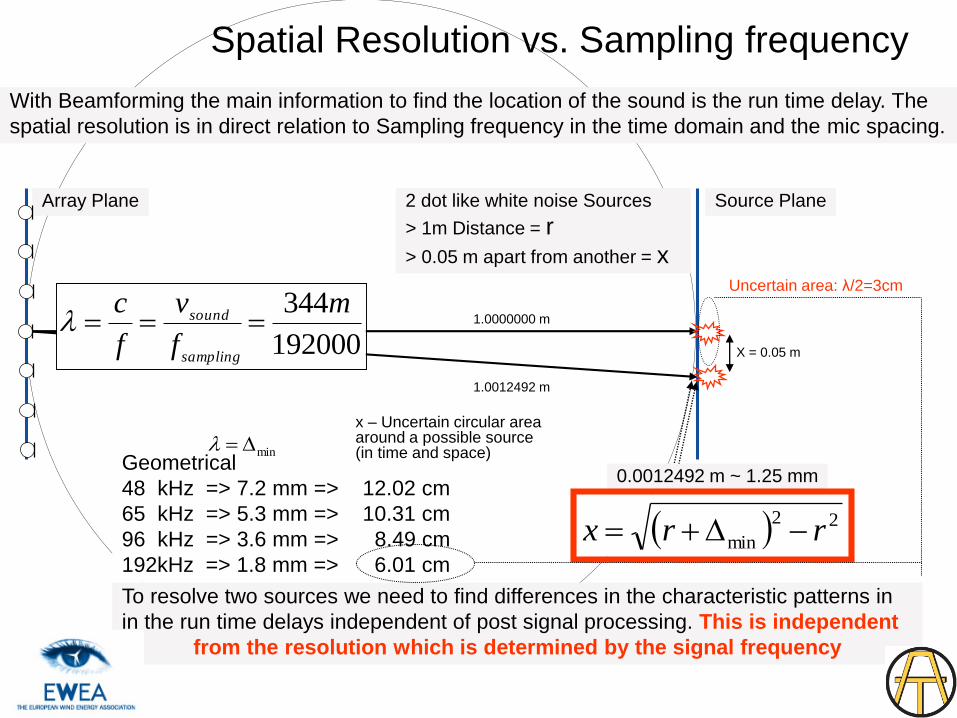
Spatial Resolution vs. Sampling frequency
Array Plane Source Plane2 dot like white noise Sources
> 1m Distance = r
> 0.05 m apart from another = x
X = 0.05 m
1.0000000 m
1.0012492 m
0.0012492 m ~ 1.25 mm
With Beamforming the main information to find the location of the sound is the run time delay. The
spatial resolution is in direct relation to Sampling frequency in the time domain and the mic spacing.
To resolve two sources we need to find differences in the characteristic patterns in
in the run time delays independent of post signal processing. This is independent
from the resolution which is determined by the signal frequency
Geometrical
48 kHz => 7.2 mm => 12.02 cm
65 kHz => 5.3 mm => 10.31 cm
96 kHz => 3.6 mm => 8.49 cm
192kHz => 1.8 mm => 6.01 cm
22
min rrx
192000
344m
f
v
f
c
sampling
sound
minx – Uncertain circular area around a possible source (in time and space)
Uncertain area: λ/2=3cm

Frequency vs. Array size
Array Size Source PlaneExample of array sizes
Low frequency limits is in direct relation to the size of the microphone array.
To resolve two uncorrelated sources we need to detect differences in the characteristic patterns in the run time delays.
Frequency
63 Hz => 5.46 m
100 Hz => 3.44 m
1 kHz => 0.34 m
10 kHz => 0.03 m
mm
f
v
Hz
sound 4.3100
344
Frequency
63 Hz => 2.73 m
100 Hz => 1.72 m
ACOUTRONIC

Spatial Resolution vs. Frequency
spatial/frequency accuracy: source diameter of 46cm, 500Hz spatial/frequency accuracy: source diameter of 22cm, 1kHz
spatial/frequency accuracy: source diameter of 10cm, 2kHz
The acoustic pictures below displays the
same dot like white noise in a distance of
1m, with a 75cm Ring Array with 32 Mics.
All pictures display have dB-contrast 3dB.
spatial/frequency accuracy: source diameter of 2cm , 10kHz

Channel number vs. Sampling frequency
16 Chanl.
48 kHz
72 Chanl.
48 kHz
32 Chanl.
48 kHz
120 Chanl.
48 kHz
ACOUTRONIC
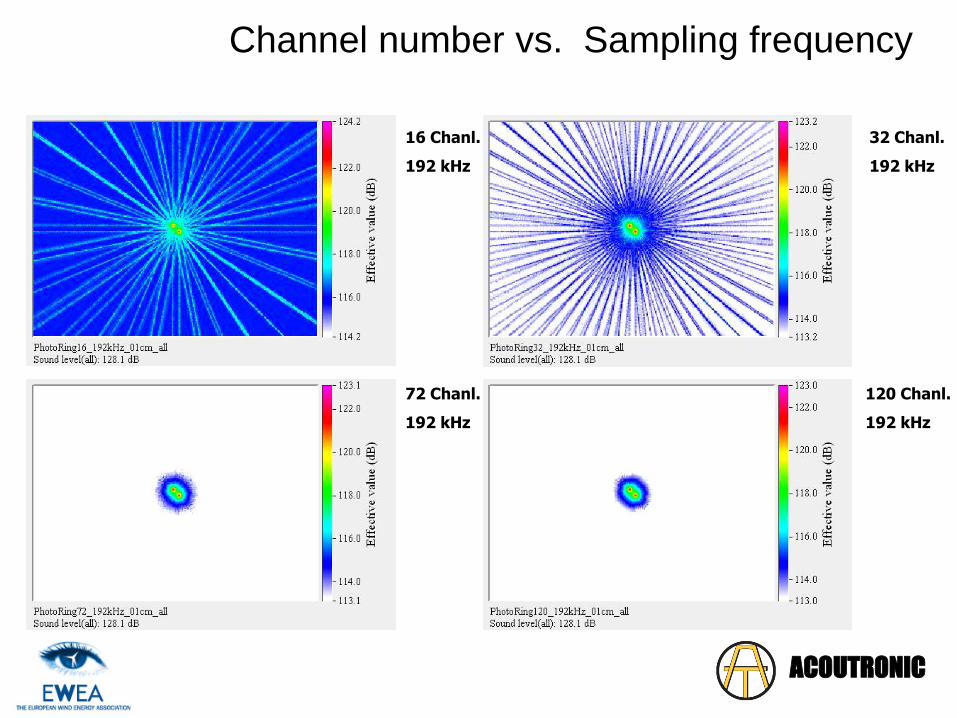
16 Chanl.
192 kHz
72 Chanl.
192 kHz
120 Chanl.
192 kHz
32 Chanl.
192 kHz
Channel number vs. Sampling frequency
ACOUTRONIC

- Acoustic Eraser – remove source
- High Dynamic Range HDR
Industrial Façade with leaks:
ACOUTRONIC
Source localization by Acoustic Camera – SW Tools
Left…: Source 66dBA, contrast 68-63(5)dBA
Middle: Erase dominating source, second source visible contrast 57-56 (1)dBA
Right..: HDR activated, contrast 68-48(20)dBA
By use of HDR we can se both dominating and other sources,
Artefacts can occur

Examples: With / Without HDR
ACOUTRONIC
Contrast: 50dB
Scale: 68–18 dB
Inbetween:-32dB
Contrast: 4dB
Scale: 68–64 dB
Between: - 2dB
Artifacts can occur
Source localization by Acoustic Camera – SW Tools
ACOUTRONIC
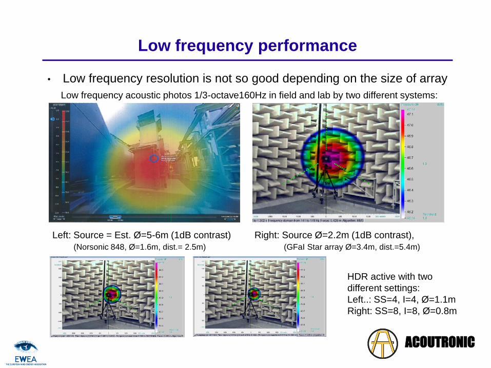
Low frequency performance
• Low frequency resolution is not so good depending on the size of array
Left: Source = Est. Ø=5-6m (1dB contrast) Right: Source Ø=2.2m (1dB contrast),
(Norsonic 848, Ø=1.6m, dist.= 2.5m) (GFaI Star array Ø=3.4m, dist.=5.4m)
Low frequency acoustic photos 1/3-octave160Hz in field and lab by two different systems:
HDR active with two
different settings:
Left..: SS=4, I=4, Ø=1.1m
Right: SS=8, I=8, Ø=0.8m
ACOUTRONIC
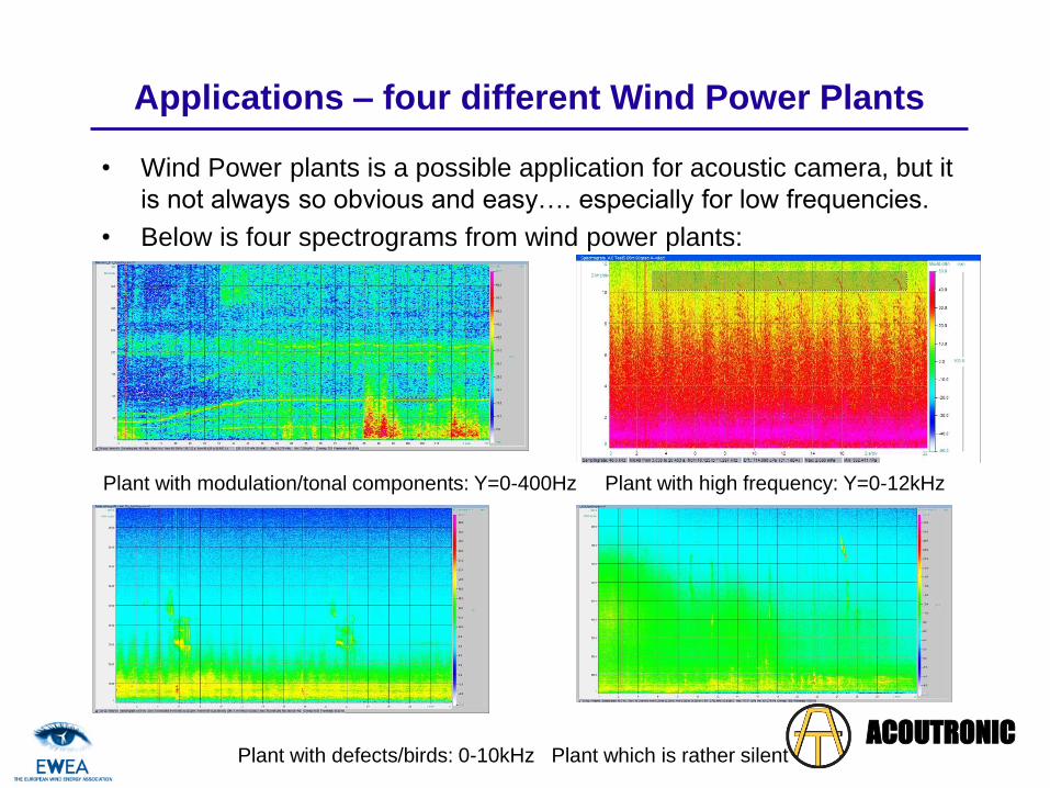
Applications – four different Wind Power Plants
• Wind Power plants is a possible application for acoustic camera, but it
is not always so obvious and easy…. especially for low frequencies.
• Below is four spectrograms from wind power plants:
Plant with modulation/tonal components: Y=0-400Hz Plant with high frequency: Y=0-12kHz
Plant with defects/birds: 0-10kHz Plant which is rather silent
ACOUTRONIC
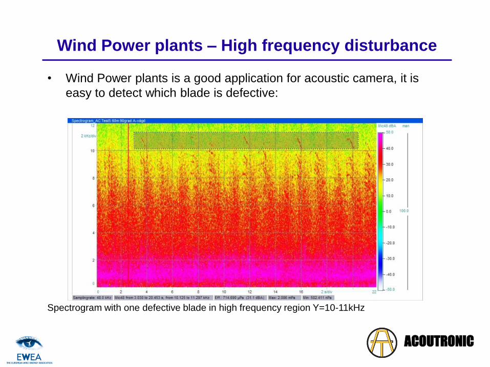
Wind Power plants – High frequency disturbance
• Wind Power plants is a good application for acoustic camera, it is
easy to detect which blade is defective:
Spectrogram with one defective blade in high frequency region Y=10-11kHz

ACOUTRONIC
GearBox problem – Wind Power Plants
• Lets zoom in on the problematic areas: Filter out the birds
Plant with defects zoom: X=5.2 to
6.7s Y=0 to 1kHz
Plant with defects - original: X=32s, Y=0 to 20kHz
Acoustic photo of defect

Low frequency/ Tonal application: 90Hz tone is ”modulated”
Zoom shows the ”90Hz” noise to be varying in amplitude
Right: Zoom of 80-100Hz:
The average spectra for 6s segment shows…..: Fundamental at 30.1Hz
Tone 1: 90.2 Hz
Tone 2: 90.7 Hz
Tone 3: 91.4 Hz
Tone 4: 92.1 Hz
ACOUTRONIC
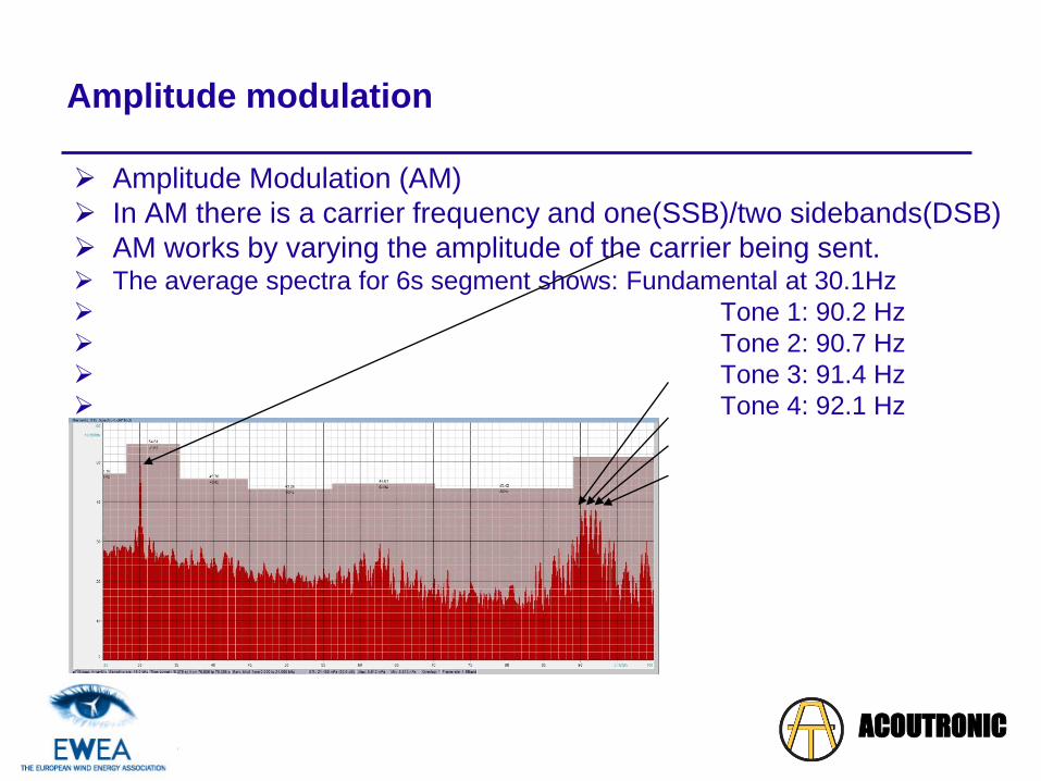
Amplitude modulation
Amplitude Modulation (AM)
In AM there is a carrier frequency and one(SSB)/two sidebands(DSB)
AM works by varying the amplitude of the carrier being sent. The average spectra for 6s segment shows: Fundamental at 30.1Hz
Tone 1: 90.2 Hz
Tone 2: 90.7 Hz
Tone 3: 91.4 Hz
Tone 4: 92.1 Hz
ACOUTRONIC

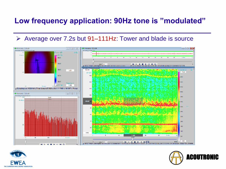
Low frequency application: 90Hz tone is ”modulated”
By analysing the envelop spectra we get modulation (F=91Hz): 91 / 432 = 0.211 Hz
Peak 1: 2x 0.211 = 0.44 Hz
Peak 2: 3x 0.211 = 0.63 Hz
Peak 3: 6x 0.211 = 1.25 Hz
Peak 4: 9x 0.211 = 1.90 Hz
ACOUTRONIC

Low frequency application: 90Hz tone is ”modulated”
Average over 7.2s between 89–111Hz: Tower is main source
ACOUTRONIC
Low frequency application: 90Hz tone is ”modulated”
Average over 7.2s but 91–111Hz: Tower and blade is source
ACOUTRONIC

Low frequency application: 90Hz tone is ”modulated”
Average but over 0.29s but 89–111Hz: Blade is source
ACOUTRONIC30 Hz tone looks like a straight line
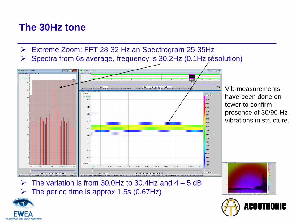
The 30Hz tone
Extreme Zoom: FFT 28-32 Hz an Spectrogram 25-35Hz
Spectra from 6s average, frequency is 30.2Hz (0.1Hz resolution)
The variation is from 30.0Hz to 30.4Hz and 4 – 5 dB
The period time is approx 1.5s (0.67Hz)
ACOUTRONIC
Vib-measurements
have been done on
tower to confirm
presence of 30/90 Hz
vibrations in structure.

The Nacelle is radiating tonal noise between 200-230Hz
MP1 &MP4: The Nacelle is radiating tones between 200 – 230Hz
During 2min run-up the noise 200-230Hz starts after 48s
The tonal components is much more present in -90° direction
There are 2 different components: at 200Hz and varying 210-230Hz
The 200Hz tone comes from nacell (rotor resonance at 200Hz)
The varying 210-230Hz tone comes from nacelle
Overtone at +90Hz = 300-320Hz comes from nacelleACOUTRONIC
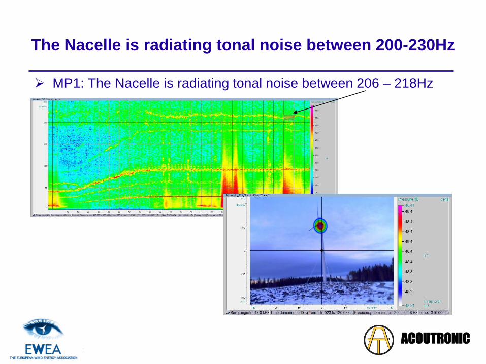
The Nacelle is radiating tonal noise between 200-230Hz
MP1: The Nacelle is radiating tonal noise between 206 – 218Hz
ACOUTRONIC

But from front view the Nacelle is not dominating
MP5: Spectrogram for 200-400Hz zoom: Marked area 207 -220Hz
MP5: Components at 200-230Hz are rather low in level
MP5: Acoustic Photo for 210-228Hz comes from blades
ACOUTRONIC

The Nacelle is radiating tonal noise between 200-320Hz
MP4: Spectrogram zoom between 200 – 350Hz MP4: The nacelle is radiating tonal noise between 207 – 227Hz
MP4: The nacelle is also radiating tones between 300 – 320 Hz (marked)
MP4: The nacelle do also have a clear tonal component around 290Hz
ACOUTRONIC
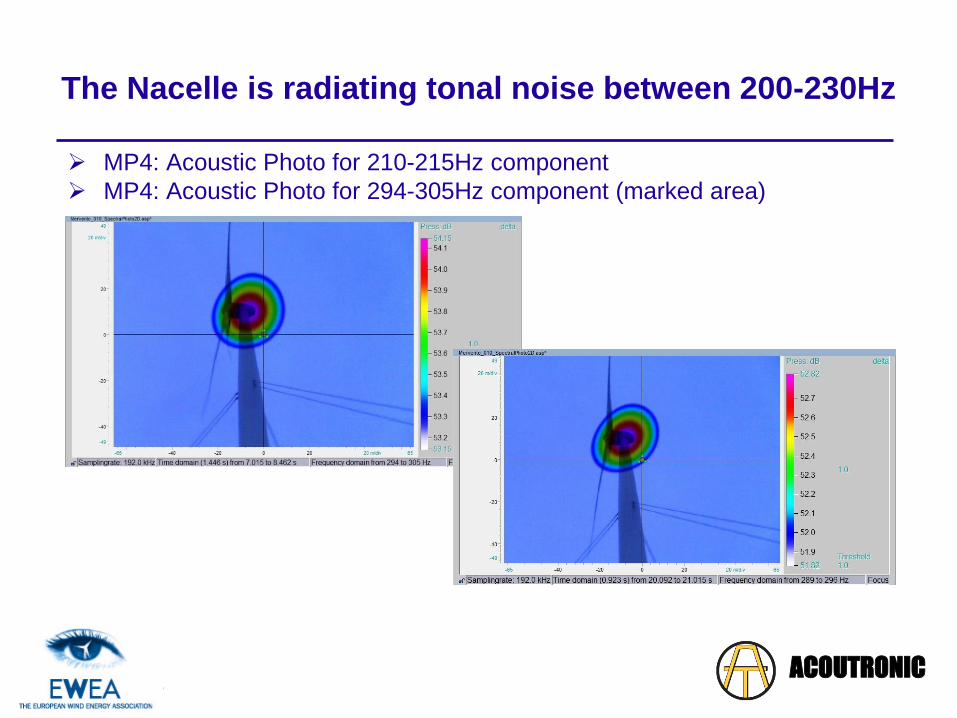
The Nacelle is radiating tonal noise between 200-230Hz
MP4: Acoustic Photo for 210-215Hz component
MP4: Acoustic Photo for 294-305Hz component (marked area)
ACOUTRONIC
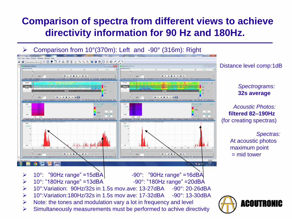
Comparison of spectra from different views to achieve
directivity information for 90 Hz and 180Hz.
Comparison from 10°(370m): Left and -90° (316m): Right
Distance level comp:1dB
Spectrograms:
32s average
Acoustic Photos:
filtered 82–190Hz
(for creating spectras)
Spectras:
At acoustic photos
maximum point
= mid tower
10°: ”90Hz range” =15dBA -90°: ”90Hz range” =16dBA
10°: ”180Hz range” =13dBA -90°: ”180Hz range” =20dBA
10°:Variation: 90Hz/32s in 1.5s mov.ave: 13-27dBA -90°: 20-26dBA
10°:Variation:180Hz/32s in 1.5s mov ave: 17-32dBA -90°: 13-30dBA
Note: the tones and modulation vary a lot in frequency and level
Simultaneously measurements must be performed to achive directivityACOUTRONIC
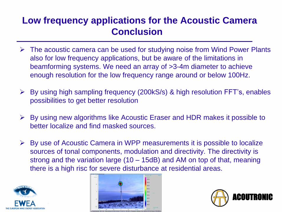
Low frequency applications for the Acoustic Camera
Conclusion
The acoustic camera can be used for studying noise from Wind Power Plants
also for low frequency applications, but be aware of the limitations in
beamforming systems. We need an array of >3-4m diameter to achieve
enough resolution for the low frequency range around or below 100Hz.
By using high sampling frequency (200kS/s) & high resolution FFT’s, enables
possibilities to get better resolution
By using new algorithms like Acoustic Eraser and HDR makes it possible to
better localize and find masked sources.
By use of Acoustic Camera in WPP measurements it is possible to localize
sources of tonal components, modulation and directivity. The directivity is
strong and the variation large (10 – 15dB) and AM on top of that, meaning
there is a high risc for severe disturbance at residential areas.
ACOUTRONIC