Low-Power Parallel Algorithms for Single Image basedObstacle Avoidance in Aerial Robots

Ian Lenz,1 Mevlana Gemici,2 and Ashutosh Saxena.11Department of Computer Science, 2Department of Electrical & Computer Engineering.

Cornell University, Ithaca, NY.Email: ianlenz@cs.cornell.edu, mcg74@cornell.edu, asaxena@cs.cornell.edu

Abstract— For an aerial robot, perceiving and avoiding obsta-cles are necessary skills to function autonomously in a clutteredunknown environment. In this work, we use a single imagecaptured from the onboard camera as input, produce obstacleclassifications, and use them to select an evasive maneuver. Wepresent a Markov Random Field based approach that modelsthe obstacles as a function of visual features and non-localdependencies in neighboring regions of the image. We performefficient inference using new low-power parallel neuromorphichardware, where belief propagation updates are done usingleaky integrate and fire neurons in parallel, while consumingless than 1 W of power. In outdoor robotic experiments, ouralgorithm was able to consistently produce clean, accurateobstacle maps which allowed our robot to avoid a wide varietyof obstacles, including trees, poles and fences.

I. INTRODUCTIONPerceiving obstacles is extremely important for an aerial

robot in order to avoid collisions. Methods based on stereovision [25], [9] are fundamentally limited by the finitebaseline between the stereo pairs [22], and fail in texturelessregions and in presence of specular reflections [4]. Activerange-finding devices (e.g., [36], [20]) are either designedfor indoor low-light environments (e.g., the Kinect [1]), orare too heavy for aerial applications. More importantly, theydemand more onboard power, which is at a premium foraerial vehicles.

In this paper, we use a single monocular camera forobstacle perception. Recent works [31], [21], [29], [32], [30],[3] have shown that it is possible to obtain depth from asingle monocular image. Multiple frames can also be used incombination to determine depth, but this approach does notwork well on an aerial robot due to camera disturbances fromrobot motion and vibrations. Here, we present an algorithmthat takes a single image as input and classifies each regionin the image as obstacle or not. We will define an obstacle asan object which the robot could not safely pass through. Thisapproach is very attractive for aerial robots because camerasare small and draw little power.

Our second key contribution is to formulate a MarkovRandom Field classification model and design fast inferencealgorithms for estimating obstacles in a new low-powerparallel hardware that implements a leaky integrate and fireneuron architecture. One implementation of such hardware[19] consumes only 45 pico-Joules per spike (see Sec-tion III for an overview). The combination of using a camera(miniature cameras that consume extremely low power are

(a) Aerial Robot. (b) Single image from camera.

(c) Initial inferred obstacle map. (d) Inferred obstacle map.

Fig. 1. We use our low-power parallel hardware for computing an obstaclemap, given a single image from the camera onboard the aerial robot. Wethen use these results to select an evasive maneuver.

available) and this hardware could allow miniature aerialrobots to successfully fly amidst obstacles even in unknownenvironments. Inference in our MRF is solved using BeliefPropagation (BP). While performing belief propagation ina traditional computer is expensive, our design allows thelow-power hardware to do so natively. Each logical clockcycle performs a full parallel update of BP. We obtain goodobstacle estimates once the BP network has converged (seeFigure 1). We then use the estimated obstacle map to selecta evasive manuever for avoiding the obstacle.

In detail, we represent the energy function of the MRFover the neuron architecture, and use spikes to propagatebeliefs during inference. Our MRF uses the logistic functionto model the local dependence of visual features to theobstacle label, where each spatial region of the image isrepresented using a different set of neurons—this allows par-allel computation. Furthermore, we use different parametersfor different spatial regions of the image [15] for improvedperformance. Finally, we induce sparsity in the parameters ofthe model to satisfy constraints on the number of parametersallowed by our hardware.

We performed extensive experiments in a variety of en-vironments, containing obstacles such as trees, fences, andpoles. In learning experiments, we obtained an averageprecision and recall of 81.9% and 93.6% respectively. In

53 outdoor robotic experiments, our algorithm was able tosuccessfully perceive obstacles in every case, and avoid themin 51 cases. The two failures were due to communicationdelays and robot drift. Some of these experiments involvedavoiding a series of obstacles of multiple types.

II. RELATED WORKIn aerial robotics, most works which perform obstacle

avoidance either make strong assumptions on precise knowl-edge of 3D location of obstacles [18], or use sensors thatare not onboard, such as GPS (together with known obstaclemap). Other work such as [8] focuses on mapping obstaclesfrom overhead images. For a small aerial robot to flyautonomously in a real environment full of obstacles, thesetechniques do not directly apply.

Navigation by labeling obstacles in images has been usedfor several ground robots. For example, Ghosh and Mulligan[7] use a ground segmentation approach for navigation, whileNabbe and Hebert [26] use ground-vertical segmentation forextending the path planning horizon for ground robots. Worksuch as [12], [33] employs learning algorithms to determineterrain traversability for ground vehicles. Michels, Saxenaand Ng [21] and Plagemann et. al. [28] attempt to determinerange directly from monocular images. However, these worksuse only a local feature based classifier for navigating aground vehicle. For an aerial robot such as ours, we areseverely constrained by onboard power, and we presentmethods that allow even a complex inference method suchas BP to be efficiently computed in low-powered hardware.

There are other works that consider single monocularimage based obstacle avoidance for aerial robots. McGeeet. al. [17] use sky segmentation for detecting obstacles,but apply only a local classifier. Soundararaj, Sujeeth andSaxena [34] and Courbon et. al. [6] use vision techniquesto navigate aerial robots, but are limited to known indoorenvironments. Bills, Chen and Saxena [5] and Zingg et. al[37] perform similar work to unknown environments, but stillhandle only a few known types of indoor environment. Onthe other hand, we consider general outdoor environments,employing learning algorithms which allow our approach tobe easily adapted to new obstacle types and integrate non-local information to enhance classification.

Vision algorithms have implemented in neural architec-tures or embedded systems, such as [13], [2], [11]. Otherworks [23], [10] used spiking neurons for basic obstacledetection and navigation. However, these approaches do notgeneralize to real-world outdoor cases.

III. NEUROMORPHIC HARDWAREOur goal is to develop algorithms for obstacle mapping

that can be implemented in low-power parallel hardware. Inparticular, we use a neuromorphic hardware platform thatcomprises a network of linear-leak integrate and fire (LLIF)artificial neurons as in [19]. The LLIF neurons representan extremely versatile high-level primitive which couples

memory and processing. More importantly, this architectureuses extremely low power, as discussed below.

Each neuron integrates the weighted synaptic inputs fromother neurons and fires if the integrated value exceeds apreset threshold. More formally, each neuron has someinteger-valued internal potential Z and binary-valued spikingoutput S. For ith neuron, S and Z update as:

Zi+t = Zit +∑

j∈N (i)

wijYjt − λi

Zit+1 = 1{Zi+t < αi}Zi+tSit+1 = 1{Zi+t ≥ αi} (1)

where N (i) are the neighbors of neuron i, wi,j indicatesthe synaptic weight from neuron j to neuron i, α indicatesneuron threshold, and λ is a constant decay. 1{...} is theindicator function, which takes the value one if its argumentis true and zero otherwise.

Since these are spiking neurons, one major restriction isthat the inputs and outputs be binary-valued. We addressthis by using representations where the spike count over aparticular time window is proportional to the value beingrepresented. Since each neuron can integrate over time, thisis still a useful representation. The expected spike rate giventhe input x is simply a ramp function with limits, as follows:

g(x, α) =

0 if x ≤ 0

x/α if 0 < x < αi

1 if x ≥ αi(2)

Cardinality constraints in hardware. To allow for a morecompact design with lower power consumption, hardwaresuch as that in [19] typically imposes a constraint on thecardinality of the weights w. That is to say, each neuron’sweights may take at most k unique nonzero values.

Power consumption in hardware. In a well-designed hard-ware platform such as [19], power consumption will beproportional to the number of spikes and the density ofconnections. In particular, the hardware in [19] takes only45 pico-Joules (pJ) per spike, and has very low quiescentpower draw in their absence.

IV. OBSTACLE CLASSIFICATIONThe primary goal of our approach is to produce an

obstacle map of sufficient quality for obstacle avoidance.This is a challenging problem, as outdoor environments areperceptually complex, with variations in obstacle appearance,lighting, background appearance, and other factors. Ourmodel will define obstacles as objects which project upwardsfrom the ground and thus present a navigational challengeto the robot. We will use the labels it produces to select anevasive maneuver for the perceived obstacles.

Our classification model is a Markov Random Field(MRF) model (e.g., see [14]), where we use an Ising pairwisepotential for modeling dependencies between neighboring

Fig. 2. Left: input images. Middle: initial classification. Right: classificationwith full MRF model with belief propagation. Initial classification resultswhich would present problems for navigation, but are greatly improved byintegrating non-local information using our MRF.

image regions. More formally, an MRF is an undirectedgraph G = (V, E), where we represent each labeled locationin the image as a vertex V , and edges E connecting neigh-boring image locations. Let Y i ∈ {−1,+1} represent thebinary labels indicating presence or absence of an obstacleat the ith location in the image, and Xi represent the inputvisual features at that location.

We model the joint conditional likelihood of the labelsgiven the features as:

P (Y |X, θ) ∝ exp (−E(Y |X, θ)) (3)

where the E(Y |X, θ) is an energy function containing threeterms:

E(Y |X, θ) = −∑i∈V

Y iA(Xi, θ)−∑

(i,j)∈E

wijYiY j + β||θ||1

(4)

The first term uses a logistic model, with θ as its parameters,to model the dependence of the label on the local visualfeatures. More formally, we model the association potentialas A(X, θ) = 2∗σ(XT θ)−1, where σ(x) = 1/(1+exp(−x))is the sigmoid function. The second term prefers neighboringlabels to be similar, with w indicating the relative importanceof the two terms. Finally, β controls the strength of an L1

regularization term on the local feature weights, which helpswith the weight cardinality constraints in the hardware.

During learning, we will be given a set of labeled examplesand our goal is to find the optimum value of the parameters.During inference, we are given a new image and our goalis to find the optimal value of Y using the LLIF neuronarchitecture.

A. LearningWe manually set parameters wij , and learn parameters θ

by maximizing the pseudo-conditional log-likelihood. We aregiven M labeled ground-truth pairs as {(Xm, Ym) : m =

1, . . . ,M}, and we learn θ∗ as:

θ∗ = argminθ

M∑m=1

E(Ym|Xm, θ) (5)

= argminθ

M∑m=1

(−∑i∈V

Y imA(Xim, θ)

)+ β||θ||1 (6)

Here, Y im indicates Y i from the mth training example,and Xi

m is similar for input features. This sub-problem isconvex, and is equivalent to solving logistic regression withan additional L1 penalty term. We vary the β parameter untilthe number of non-zero weights fits within what is allowedin the hardware.B. Inference

The goal of inference is to find an optimal value for thelabel estimates Y , given features X and parameters θ:

Y ∗ = arg maxY

P (Y |X, θ) (7)

Our inference algorithm is based on loopy belief propa-gation [27], [24]. In order to derive the update rule for nodei, we assume that the values of the other nodes are knownand compute the messages as follows:

ψ(Xi) = σ(θTXi) (8)

µi(Xi) = ψ(Xi)

∏(i,j)∈E

µj(Xj)wij (9)

P (Y i = 1|X) = µi(Xi) (10)

Our goal is to perform obstacle avoidance in new envi-ronments, and the product above may give zero probabilityof being an obstacle if any of terms is zero. This is notpreferable, and we need to account for such cases. Followingideas of additive smoothing in statistics [35], we include anadditive smoothing term in ψ and µ. This is a small constantfactor ε added to each function. Denote the versions of thesefunctions with additive smoothing as ψs and µs.

If we consider these update equations in log-space, theybecome sum of weighted terms, and thereby can be imple-mented in neuromorphic hardware (Eqn. 1). In such a case,the additive smoothing term becomes a constant lower boundon the log probability terms. Thus, in log-space, we have:

logψs(Xi) = max(log ε, log σ(θTXi)) (11)

logµs,i(Xi) = max

(log ε, logψs(X

i)

+∑

(i,j)∈E

wij logµs,j(Xj))

(12)

To implement this in hardware, we will use one neuron eachto represent ψs(Xi) and µs,i(Xi) for each node. Each ψ unitwill take input in spike-rate from local features, weighted asθ. Each µ unit will take input from the corresponding ψ unitand neighboring µ units, weighted as w.

The log-sigmoid ψs term can be approximated as a linearfunction which saturates at 0. With the lower bound from

the additive smoothing function, this becomes a scaled andshifted version of Eqn. 2. We will refer to the version ofg(x, α) adjusted to fit the log-sigmoid function as gψ(x).logµs,i(X

i) is also well approximated by a thresholdedlinear function, and can thus also be modeled by g(x, α),as gµ(x). In both cases, α is fixed to some value whichgives the best fit. The equations for our system are then:

logψs(Xi) = gψ(θ

TXi)− logZψ (13)

logµs,i(Xi) = gµ(wiiψs(X

i) +∑

(i,j)∈E

wijµs,j(Xj))− logZµ

(14)

Where the Z’s are two separate constants, necessary toinclude here to preserve exact equality, but unnecessary toimplement in hardware since relative values are preserved.Except for the error introduced by approximating the log-sigmoid function with gψ(x) and discretization, this is ex-actly Eqn. 12. To infer optimal values for Y , we can simplythreshold the gµ terms once the network has converged.C. Visual Features

Our basic features are a standard set of texture filterresponses, similar to those in [16]. They consist of orientededge filters (in our case, Gabor filters) and center-surroundfilters (difference-of-Gaussian filters) as shown in Figure 3.We also include color information in the form of patch-averaged RGB values in our feature set. In addition toraw filter responses, we include the absolute value of theseresponses and the maximum and average of this absolutevalue over a local area.

We found it difficult to design features which fit the hard-ware constraints of [19], so the features given here do not.They do, however, rely only on simple local computations,and thus are amenable to efficient implementation in circuitryor parallel hardware. Only features given nonzero weightsby some classifier would need to be implemented in thishardware, significantly reducing complexity.

Fig. 3. Our filter set, which includes two scales of Gabor filters at sixorientations and two scales of difference-of-Gaussian filters.

D. Spatially-varying models and multiple models

Often the statistics of the dependence of the obstacles onthe visual features varies with their location in the image[15]. For example, while leaves on the trees are typicallyobstacles, they are not if they fall on the ground in theFall season. Thus our parameters θ should be different for

different rows in the image. In order to do so, we dividethe image vertically into three equally sized areas. This isequivalent to considering a separate θi for each i ∈ V , andtying weights within regions. By dividing the classificationas such, each region can have a different feature set. Tyingthe parameters of these different models helps to avoidover-fitting. Since our neuron architecture is distributed fordifferent spatial regions in the image, each neuron gets theappropriate synaptic weights depending on which region inthe image it is representing.

To detect multiple visually different obstacle classes, wetrain a model for each class and use the combined outputof these models. In order to exercise maximum caution, wecombine outputs using the logical OR of the results, ie ifany classifier classifies a region as obstacle, it is consideredto be an obstacle for purposes of navigation.

Since our algorithms run natively in parallel hardware,neither of these changes require a change to the architectureor cause an increase in runtime.

E. Tuning for Power ConsumptionOne major strength of the hardware described in [19]

is that its power consumption can be estimated a priorifrom simulation with high accuracy. This is because powerconsumption in this hardware is determined largely by twofactors: a) connection density and b) spike count. Whilea) is fixed for a particular local connection pattern, b) canchange drastically depending on the relative weight betweenlocal classifier estimates and neighboring labels, as well asneuron threshold and decay. In particular, faster convergenceof the MRF model in terms of hardware timesteps cansignificantly reduce power consumption, as the model can beterminated earlier and thus generates fewer spikes. Therefore,in practice, we tune our models for a tradeoff between powerand accuracy, aiming to produce results which produce fewerspikes while still yielding results which would be useful forobstacle avoidance.

In practice, we obtained good performance in terms ofboth accuracy and performance for the following parametersettings for each neuron:• wii: set slightly below α (firing threshold).• wij : set to a small local connectivity pattern (4- or 8-

way), with uniform weights set to 10-20% of α.• λ (decay): set to 5-10% of α.

V. OBSTACLE AVOIDANCE MANUEVERSThe goal of our obstacle avoidance algorithm is to avoid

obstacles in near to mid-range (e.g., about 2m to 10m). Ourmotion selection algorithm uses a library of paired motionsand visual-space masks. If less than some threshold’s worthof pixels within a masked area are labeled as obstacles, thecorresponding motion is considered to be safe. The effectsof sweeping this threshold are shown in Figure 6. A fixedpreference order is used to select motions in cases wheremore than one is found to be safe.

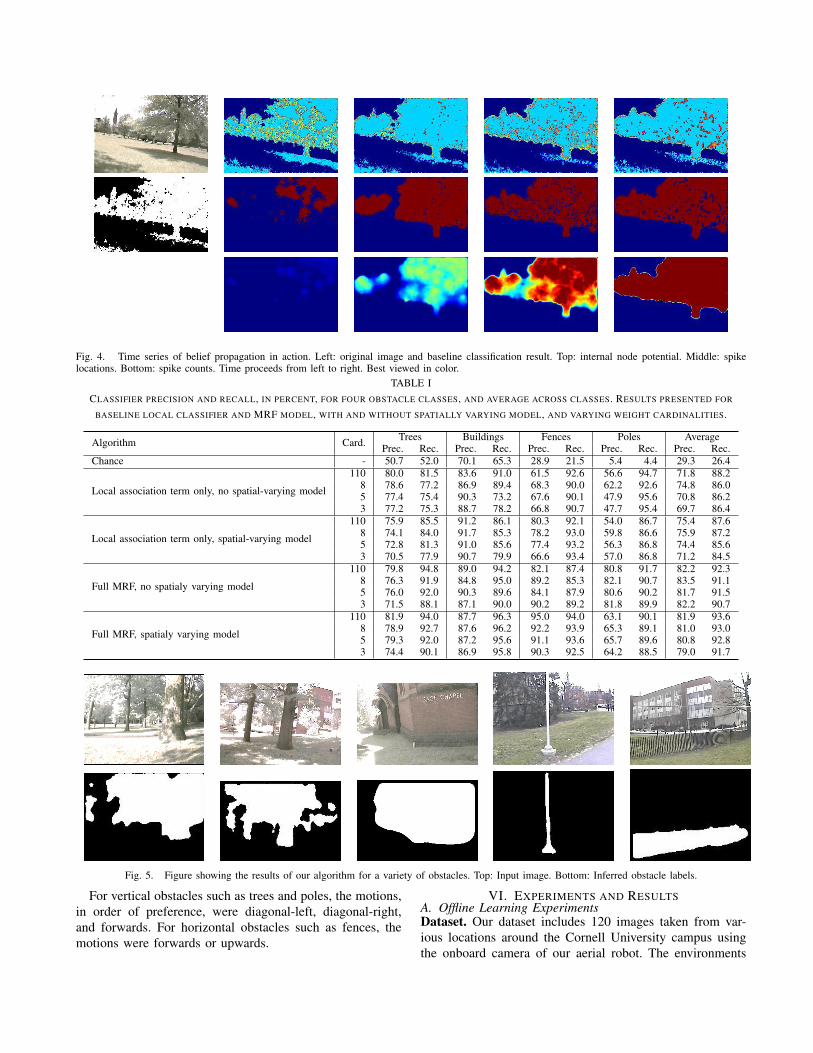
Fig. 4. Time series of belief propagation in action. Left: original image and baseline classification result. Top: internal node potential. Middle: spikelocations. Bottom: spike counts. Time proceeds from left to right. Best viewed in color.

TABLE ICLASSIFIER PRECISION AND RECALL, IN PERCENT, FOR FOUR OBSTACLE CLASSES, AND AVERAGE ACROSS CLASSES. RESULTS PRESENTED FOR

BASELINE LOCAL CLASSIFIER AND MRF MODEL, WITH AND WITHOUT SPATIALLY VARYING MODEL, AND VARYING WEIGHT CARDINALITIES.

Algorithm Card. Trees Buildings Fences Poles AveragePrec. Rec. Prec. Rec. Prec. Rec. Prec. Rec. Prec. Rec.

Chance - 50.7 52.0 70.1 65.3 28.9 21.5 5.4 4.4 29.3 26.4

Local association term only, no spatial-varying model

110 80.0 81.5 83.6 91.0 61.5 92.6 56.6 94.7 71.8 88.28 78.6 77.2 86.9 89.4 68.3 90.0 62.2 92.6 74.8 86.05 77.4 75.4 90.3 73.2 67.6 90.1 47.9 95.6 70.8 86.23 77.2 75.3 88.7 78.2 66.8 90.7 47.7 95.4 69.7 86.4

Local association term only, spatial-varying model

110 75.9 85.5 91.2 86.1 80.3 92.1 54.0 86.7 75.4 87.68 74.1 84.0 91.7 85.3 78.2 93.0 59.8 86.6 75.9 87.25 72.8 81.3 91.0 85.6 77.4 93.2 56.3 86.8 74.4 85.63 70.5 77.9 90.7 79.9 66.6 93.4 57.0 86.8 71.2 84.5

Full MRF, no spatialy varying model

110 79.8 94.8 89.0 94.2 82.1 87.4 80.8 91.7 82.2 92.38 76.3 91.9 84.8 95.0 89.2 85.3 82.1 90.7 83.5 91.15 76.0 92.0 90.3 89.6 84.1 87.9 80.6 90.2 81.7 91.53 71.5 88.1 87.1 90.0 90.2 89.2 81.8 89.9 82.2 90.7

Full MRF, spatialy varying model

110 81.9 94.0 87.7 96.3 95.0 94.0 63.1 90.1 81.9 93.68 78.9 92.7 87.6 96.2 92.2 93.9 65.3 89.1 81.0 93.05 79.3 92.0 87.2 95.6 91.1 93.6 65.7 89.6 80.8 92.83 74.4 90.1 86.9 95.8 90.3 92.5 64.2 88.5 79.0 91.7

Fig. 5. Figure showing the results of our algorithm for a variety of obstacles. Top: Input image. Bottom: Inferred obstacle labels.

For vertical obstacles such as trees and poles, the motions,in order of preference, were diagonal-left, diagonal-right,and forwards. For horizontal obstacles such as fences, themotions were forwards or upwards.

VI. EXPERIMENTS AND RESULTSA. Offline Learning ExperimentsDataset. Our dataset includes 120 images taken from var-ious locations around the Cornell University campus usingthe onboard camera of our aerial robot. The environments

include four types of obstacles: trees, buildings, light poles,and fences. The dataset includes 63 images of trees, 45 ofbuildings, 10 of poles and 10 of fences. We used 80% of theimages for training and 20% for testing.Belief Propagation. During inference, our BP system ex-hibits distinct phases of operation as seen in Figure 4. First,there is a warm-up phase where nodes with high values ofclassifier output build up energy. Eventually, some of thesenodes’ local potential exceeds their thresholds and they fire,spreading energy to neighboring nodes which may also firein response. Spikes begin to propagate across the network,which finally reaches a steady state from which inferredclassification labels are determined.Results. Table I shows the performance of our algorithm. Wepresent comparisons with different models. First, we considera model with only the association term, i.e., equivalent to alocal logistic classifier. Second, we also compare the effectsof training several spatially varying models. We compare theeffects of reducing the cardinality of local classifier weightsas well. Similar baseline results were observed using SVM.

Our results show that the spiking neuron based BP systemhas proven very effective in producing cleaner, more usableresults for obstacle avoidance, as compared to baselineresults using the local logistic term only. Since our featureset contains edge and center-surround filter responses, localclassifier estimates are generally stronger at obstacle edges.BP propagates these inwards, allowing the entire obstacleto be classified, causing increases in recall of as muchas 17%. This propagation behavior can sometimes smoothedges of perceived obstacles slightly, as seen in many casesin Figure 5, causing a slight decrease in precision offset bygains elsewhere.

Most clear areas contain no strong local values and thusdo not generate an initial spike, while true positive regionsalmost always do. This allows the system to avoid some falsepositive cases present in the baseline results. For obstacleavoidance purposes, recall is much more important thanprecision, and errors near an obstacle are less important thanfalse positives in otherwise clear areas.

In order to evaluate the performance of our algorithm forobstacle avoidance purposes, we discretized the lower regionof each test image into a 3x5 grid of cells, and considereda cell to be ground-truth occupied if it contained at least10% ground-truth obstacles. We produced the curve shownin Figure 6 by sweeping thresholds for occupancy ratios. Ouralgorithm outperforms the baseline in all cases. The mostsignificant improvement is for high values of recall, whichare necessary for safe obstacle avoidance. Results presentedare for trees, results for other classes were similar.Weight Cardinality Limitations. Reducing the number offeatures available to the classifier decreases performanceon average, producing particularly significant decreases forvaried obstacles such as trees. However, with BP, the resultsare generally comparable for all weight cardinalities. This

Fig. 6. Precision-recall curve for cell-based error metric, which demon-strates improvements over baseline results for navigation purposes.

Fig. 7. Classification results for a tree trunk classifier using our algorithm,on the same tree under very different lighting conditions.

demonstrates that BP is able to resolve the errors producedby restricting weight cardinality, making it an ideal choiceas an inference algorithm in neuromorphic hardware whichimposes that constraint.Spatially-varying models. Baseline results were improvedby spatially-varying models in most cases, and full MRFresults were improved in all cases except poles. This suggeststhat spatially varying models are useful in most cases, butmight be foregone for obstacles with spatially consistentvisual appearance such as poles.Performance in different environments. Since our al-gorithm uses supervised learning to learn local classifierweights, it is easily adapted to new obstacle classes. Thefour classes presented here are very visually different, yetour model is able to detect obstacles effectively in each.Our model was also able to handle variations in lightingand obstacle appearance (such as leaves falling off the trees).Figure 7 shows an example of a tree trunk classifier using ouralgorithm performing effectively under a variation in lightingconditions.B. Robotic Experiments in Real Environments

We performed obstacle avoidance experiments on ouraerial robot platform, an AirRobot with a single onboard

Fig. 8. Our aerial robot avoiding a fence and a pole in sequence. Left: Overhead map of area, red indicates obstacles avoided, blue robot path. Robotstarted at the blue dot, behind and below the level of the fence, moved upwards to a safe altitude, and proceeded over the fence and through the clear area.It then stopped at the pole, detected it as an obstacle, moved diagonally to the right to avoid it, and then forwards again through the following clear area.

Fig. 9. AirRobot avoiding obstacles based on our classification results(robot circled in red in cases where it’s difficult to see)

TABLE IIROBOTIC EXPERIMENT RESULTS IN OUTDOOR ENVIRONMENTS. ERROR

RATES PRESENTED FOR CLASSIFICATION, MOTION EXECUTION, AND

OVERALL SUCCESSFUL AVOIDANCE

Type Obstacles Tests Success RateClass. Motion Overall

Trees 3 20 100.0% 95.0% 95.0%Fences 3 25 100.0% 100.0% 100.0%Poles 2 8 100.0% 87.5% 87.5%Total 8 53 100.0% 96.2% 96.2%

camera and an onboard IMU for stabilization.1 Since thehardware described in [19] is still in production, processingwas done using an offboard laptop computer running aMATLAB simulation of the hardware. Due to transmissionlatency and a lack of the necessary parallelism, this limitedus to classifying a single image at a time, then taking a largestep with the robot.

For each experiment, the robot was driven to a hoveringposition roughly 2-10 meters from the obstacle. Using therobot’s IMU, we determined when it was in a stable, levelpose, then captured an image from its onboard camera.

1Because of funding agency’s restrictions, we are not allowed to disclosemore detailed specifications of our system.

This image was transmitted to the laptop, which performedthe classification described in Section IV, using a classifiertrained for the appropriate obstacle class. We then used thealgorithm described in Section V to select an appropriateavoidance maneuver. The robot then executed a predeter-mined, fixed motion plan based on the maneuver chosen.

In Table II, we report three types of success-rates: “classi-fication”: when the obstacle classification was correct, “mo-tion”: when the computed obstacle avoidance maneuver wascorrect, and “overall”: when the robot successfully executedthe maneuver avoiding the obstacle.

In all the experiments in Table II, classification resultsfrom our model were of sufficient accuracy to allow thecontroller described in Section V to properly select a safemotion. Our model identified both foreground obstacles andclear areas consistently in these experiments.

As seen in Figure 9, our algorithm worked even inenvironments with visually cluttered backgrounds such asbuildings and background trees. While these backgrounds didcause some false positives, as seen in some cases in Figure 5,these were only in the top region of the image, which wasnot considered by the controller. Since our algorithm worksat visual range, it was able to perceive obstacles from longdistances, allowing the robot to make large, predeterminedmotions to avoid them.

Some obstacles encountered were semi-transparent, suchas the fence in the bottom row of Figure 9. Even though thevisual appearance of the fence varied depending on viewingangle and background, and the fence exhibited specularreflections in some places, our algorithm was able to producean extremely clean labeling of the fence as seen in Figure 5.

We also performed an experiment where the robot avoidedmultiple classes of obstacles in sequence. The classificationmodels for fences and poles were run in parallel, and onlymotions determined to be safe by both were considered. Therobot was re-oriented to its goal travel direction after eachmotion. The robot was able to travel roughly 25 meters whileavoiding obstacles, as shown in Figure 8. This approach was

able to produce good results because the models were ableto correctly report a lack of foreground obstacles when therewere none, allowing only the classifiers for which foregroundobstacles were present to dictate maneuver selection.

Video showing our robot avoiding obstacles using ouralgorithm is submitted as supplementary material, and is alsoavailable at: http://mav.cs.cornell.edu

VII. CONCLUSIONSWe presented a learning algorithm that takes as input a sin-

gle image and outputs an obstacle map. Our algorithm usesa Markov Random Field to model the mapping from visualfeatures to obstacles and the relations between neighboringregions in the image. We use parallel neuromorphic hardwarefor performing inference in the model. This hardware is well-suited for aerial robots because of its extremely low powerrequirements. Our MRF model also considers the cardinalityconstraints of the synaptic weights, and tries to minimize thepower requirements for inference by minimizing the numberof spikes. In upcoming hardware, our algorithms would allowseveral frames per second to be processed, while consumingless than 1 W of power.

We evaluated our algorithms in both learning experimentsand robotic experiments. In learning experiments, our MRFmodel made significant improvements in classifier accuracyboth quantitatively and qualitatively for the purpose of obsta-cle avoidance. In robotic experiments, our algorithm was ableto correctly identify the locations of forgeround obstacles inall tests, allowing the robot to select an evasive maneuver toavoid them. Some of these tests involved multiple obstaclesof different classes in sequence, demonstrating that inferenceresults from multiple models can be effectively combined.

VIII. ACKNOWLEDGEMENTSWe would like to thank Dharmendra Modha, Shyamal

Chandra, Thomas Zimmerman, Stefano Carpin, Steve Esser,Myron Flickner, Jerry Yeh, and Dale Cassidy for usefuldisussions, and Jasdeep Hundal and Brian Wojcik for theirhelp with experiments. This work was partially supported byDARPA under grant #HR0011-09-C-0002 and by Alfred P.Sloan research fellowship to one of us (Saxena).

REFERENCES

[1] A. Bachrach, S. Prentice, R. He, and N. Roy. Range - robustautonomous navigation in gps-denied environments. Journal of FieldRobotics, 28(5):644–666, 2011.

[2] C. Bartolozzi, F. Rea, C. Clercq, M. Hofstatter, D. Fasnacht, G. In-diveri, and G. Metta. Embedded neuromorphic vision for humanoidrobots. In ECVW, 2011.

[3] D. Batra and A. Saxena. Learning the right model: Efficient max-margin learning in laplacian crfs. In CVPR, 2012.

[4] D. Bhat and S. Nayar. Stereo in the presence of specular reflection.In ICCV, 1995.

[5] C. Bills, J. Chen, and A. Saxena. Autonomous mav flight in indoorenvironments using single image perspective cues. In ICRA, 2011.

[6] J. Courbon, Y. Mezouar, N. Guenard, and P. Martinet. Visualnavigation of a quadrotor aerial vehicle. In IROS, 2009.

[7] S. Ghosh and J. Mulligan. A segmentation guided label propagationscheme for autonomous navigation. In ICRA, 2010.

[8] H. K. Heidarsson and G. S. Sukhatme. Obstacle detection from over-head imagery using self-supervised learning for autonomous surfacevehicles. In IROS, 2011.

[9] S. Hrabar. 3d path planning and stereo-based obstacle avoidance forrotorcraft uavs. In IROS, 2008.

[10] S. B. i Badia, P. Pyk, and P. F. M. J. Verschure. A fly-locustbased neuronal control system applied to an unmanned aerial vehicle:the invertebrate neuronal principles for course stabilization, altitudecontrol and collision avoidance. IJRR, 26(7):759–772, 2007.

[11] T. Jochem, D. Pomerleau, and C. Thorpe . Vision-based neural networkroad and intersection detection and traversal. In IROS, 1995.

[12] D. Kim, J. Sun, S. Min, O. James, M. Rehg, and A. F. Bobick.Traversability classification using unsupervised on-line visual learningfor outdoor robot navigation. In ICRA, 2006.

[13] A. Konno, R. Uchikura, T. Ishihara, T. Tsujita, T. Sugimura,J. Deguchi, M. Koyanagi, and M. Uchiyama. Development of a highspeed vision system for mobile robots. In IROS, 2006.

[14] S. Kumar and M. Hebert. Discriminative random fields: A discrimi-native framework for contextual interaction in classification. In ICCV,2003.

[15] C. Li, A. Saxena, and T. Chen. θ-mrf: Capturing spatial and semanticstructure in the parameters for scene understanding. In NIPS, 2011.

[16] J. Malik, S. Belongie, J. Shi, and T. Leung. Textons, contours andregions: Cue integration in image segmentation. In ICCV, 1999.

[17] T. McGee, R. Sengupta, and K. Hedrick. Obstacle detection for smallautonomous aircraft using sky segmentation. In ICRA, 2005.

[18] D. Mellinger, N. Michael, and V. Kumar. Trajectory generation andcontrol for precise aggressive maneuvers with quadrotors. In ISER,Dec 2010.

[19] P. Merolla, J. Arthur, F. Akopyan, N. Imam, R. Manohar, andD. Modha. A digital neurosynaptic core using embedded crossbarmemory with 45pj per spike in 45nm. In CICC, 2011.

[20] T. Merz and F. Kendoul. Beyond visual range obstacle avoidance andinfrastructure inspection by an autonomous helicopter. In IROS, 2011.

[21] J. Michels, A. Saxena, and A. Y. Ng. High speed obstacle avoidanceusing monocular vision and reinforcement learning. In ICML, 2005.

[22] R. Moore, S. Thurrowgood, D. Bland, D. Soccol, and M. Srinivasan.A stereo vision system for uav guidance. In IROS, 2009.

[23] R. Mudra, R. Hahnloser, and R. J. Douglas. Neuromorphic activevision used in simple navigation behavior for a robot. In Proc. 7thInt. Conf. On Microelectronics for Neural Networks, pages 7–9, 1999.

[24] K. P. Murphy, Y. Weiss, and M. I. Jordan. Loopy belief propagationfor approximate inference: An empirical study. In UAI, 1999.

[25] I. Na, S. H. Han, and H. Jeong. Stereo-based road obstacle detectionand tracking. In ICACT, 2011.

[26] B. Nabbe and M. Hebert. Extending the path-planning horizon.volume 26, pages 997–1024, 2007.

[27] J. Pearl. Fusion, propagation, and structuring in belief networks. Artif.Intell., 29(3):241–288, 1986.

[28] C. Plagemann, F. Endres, J. M. Hess, C. Stachniss, and W. Burgard.Monocular range sensing: A non-parametric learning approach. InICRA, 2008.

[29] A. Saxena, S. Chung, and A. Ng. Learning depth from singlemonocular images. In NIPS, 2005.

[30] A. Saxena, S. Chung, and A. Ng. 3-d depth reconstruction from asingle still image. IJCV, 76(1):53–69, 2008.

[31] A. Saxena, M. Sun, and A. Ng. Make3d: Learning 3d scene structurefrom a single still image. PAMI, 2009.

[32] A. Saxena, M. Sun, and A. Y. Ng. Make3d: Depth perception from asingle still image. In AAAI, 2008.

[33] B. Sofman, E. L. Ratliff, J. A. D. Bagnell, J. Cole, N. Vandapel,and A. T. Stentz. Improving robot navigation through self-supervisedonline learning. Journal of Field Robotics, 23(12), 2006.

[34] S. P. Soundararaj, A. K. Sujeeth, and A. Saxena. Autonomous indoorhelicopter flight using a single onboard camera. In IROS, 2009.

[35] V. Vapnik. Statistical Learning Theory. John Wiley and Sons, 1998.[36] K. M. Wurm, R. Kummerle, C. Stachniss, and W. Burgard. Improving

robot navigation in structured outdoor environments by identifyingvegetation from laser data. In IROS, 2009.

[37] S. Zingg, D. Scaramuzza, S. Weiss, and R. Siegwart. Mav navigationthrough indoor corridors using optical flow. In ICRA, 2010.