low-rank training of deep neural networks for emerging

LOW-RANK TRAINING OF DEEP NEURAL NETWORKSFOR EMERGING MEMORY TECHNOLOGY

Albert Gural 1 Phillip Nadeau 2 Mehul Tikekar 2 Boris Murmann 1

ABSTRACTThe recent success of neural networks for solving difficult decision tasks has incentivized incorporating smartdecision making “at the edge.” However, this work has traditionally focused on neural network inference, ratherthan training, due to memory and compute limitations, especially in emerging non-volatile memory systems, wherewrites are energetically costly and reduce lifespan. Yet, the ability to train at the edge is becoming increasinglyimportant as it enables real-time adaptability to device drift and environmental variation, user customization, andfederated learning across devices. In this work, we address two key challenges for training on edge devices withnon-volatile memory: low write density and low auxiliary memory. We present a low-rank training scheme thataddresses these challenges while maintaining computational efficiency. We then demonstrate the technique on arepresentative convolutional neural network across several adaptation problems, where it out-performs standardSGD both in accuracy and in number of weight writes.

1 INTRODUCTION

Deep neural networks have shown remarkable performanceon a variety of challenging inference tasks. As the energyefficiency of deep-learning inference accelerators improves,some models are now being deployed directly to edge de-vices to take advantage of increased privacy, reduced net-work bandwidth, and lower inference latency. Despite edgedeployment, training happens predominately in the cloud.This limits the privacy advantages of running models on-device and results in static models that do not adapt toevolving data distributions in the field.

Efforts aimed at on-device training address some of thesechallenges. Federated learning aims to keep data on-deviceby training models in a distributed fashion (Konecny et al.,2016). On-device model customization has been achievedby techniques such as weight-imprinting (Qi et al., 2018),or by retraining limited sets of layers. On-chip training hasalso been demonstrated for handling hardware imperfections(Zhang et al., 2017; Gonugondla et al., 2018). Despitethis progress with small models, on-chip training of largermodels is bottlenecked by the limited memory size andcompute horsepower of edge processors.

Emerging non-volatile (NVM) memories such as resistiverandom access memory (RRAM) have shown great promise

1Department of Electrical Engineering, Stanford Univer-sity, Stanford, USA 2Analog Devices Incorporated, Norwood,Massachusetts, USA. Correspondence to: Albert Gural <[email protected]>.

for energy and area-efficient inference (Yu, 2018). In Fig-ure 1, NVM used in solution C is able to solve the weight-movement energy drawbacks of traditional solution A whilealso alleviating the chip area drawbacks of solution B. Thebenefits offered by NVM for neural network inference sug-gest it may become an important component of future smartedge devices. However, while solution C offers advantagesfor inference, it can make training even more difficult. On-chip training requires a large number of writes to the mem-ory, and RRAM writes cost significantly more energy thanreads (e.g., 10.9 pJ/bit versus 1.76 pJ/bit (Wu et al., 2019)).Additionally, RRAM endurance is on the order of 106 writes(Grossi et al., 2019), shortening the lifetime of a device dueto memory writes for on-chip training. In anticipation ofgrowing numbers of inference-optimized NVM-based edgedevices, we ask what can be done to enable training as well.

In this paper, we present an online training scheme amenableto NVM memory solutions. Our contributions are (1) analgorithm called Low Rank Training (LRT), and its analysis,which addresses the two key challenges of low write densityand low auxiliary memory; (2) two techniques “gradientmax-norm” and “streaming batch norm” to help trainingspecifically in the online setting; (3) a suite of adaptationexperiments to demonstrate the advantages of our approach.

2 RELATED WORK

Efficient training for resistive arrays. Several works haveaimed at improving the efficiency of training algorithms onresistive arrays. Of the three weight-computations required

arX

iv:2

009.

0388

7v2

[cs

.LG

] 1

5 Ju

l 202

1

Low Rank Training of Deep Neural Networks for Emerging Memory Technology

Chip

BufferSRAM MMU

WeightsDRAM

data

Chip

BufferSRAM MMU

WeightsFlash

Chip

BufferSRAM MMU

WeightsRRAM

Solution A Solution B Solution C

Figure 1. Three edge inference solutions are illustrated. SolutionA is the approach used in modern devices. Large DNN memoryis stored in off-chip DRAM, resulting in large weight movementenergy costs. Moving weight memory on-chip reduces weightmovement costs, but can increase chip area substantially, as shownin solution B. NVM, such as RRAM shown in solution C, isspatially dense and alleviates the challenges of solutions A and B.

in training (forward, backprop, and weight update), weightupdates are the hardest to parallelize using the array struc-ture. Stochastic weight updates (Gokmen & Vlasov, 2016)allow programming of all cells in a crossbar at once, asopposed to row/column-wise updating. Online Manhattanrule updating (Zamanidoost et al., 2015) can also be usedto update all the weights at once. Several works have pro-posed new memory structures to improve the efficiency oftraining (Soudry et al., 2015; Ambrogio et al., 2018). Thenumber of writes has also been quantified in the context ofchip-in-the-loop training (Yu et al., 2016).

Distributed gradient descent. Distributed training in thedata center is another problem that suffers from expensiveweight updates. Here, the model is replicated onto manycompute nodes and in each training iteration, the mini-batchis split across the nodes to compute gradients. The dis-tributed gradients are then accumulated on a central nodethat computes the updated weights and broadcasts them.These systems can be limited by communication bandwidth,and compressed gradient techniques (Aji & Heafield, 2017)have therefore been developed. In Lin et al. (2017), thegradients are accumulated over multiple training iterationson each compute node and only gradients that exceed athreshold are communicated back to the central node. In thecontext of on-chip training with NVM, this method helpsreduce the number of weight updates. However, the gradi-ent accumulator requires as much memory as the weightsthemselves, which negates the density benefits of NVM.

Low-Rank Training. Our work draws heavily from previ-ous low-rank training schemes that have largely been de-veloped for use in recurrent neural networks to uncouplethe training memory requirements from the number of timesteps inherent to the standard truncated backpropagation

through time (TBPTT) training algorithm. Algorithms de-veloped since then to address the memory problem includeReal-Time Recurrent Learning (RTRL) (Williams & Zipser,1989), Unbiased Online Recurrent Optimization (UORO)(Tallec & Ollivier, 2017), Kronecker Factored RTRL (KF-RTRL) (Mujika et al., 2018), and Optimal Kronecker Sums(OK) (Benzing et al., 2019). These latter few techniquesrely on the weight gradients in a weight-vector product look-ing like a sum of outer products (i.e., Kronecker sums) ofinput vectors with backpropagated errors. Instead of storinga growing number of these sums, they can be approximatedwith a low-rank representation involving fewer sums.

3 TRAINING NON-VOLATILE MEMORY

The meat of most deep learning systems are many weightmatrix - activation vector products W · a. Fully-connected (dense) layers use them explicitly: a[`] =σ(W [`]a[`−1] + b[`]

)for layer `, where σ is a non-linear

activation function (more details are discussed in detail inAppendix B.1). Recurrent neural networks use one or manymatrix-vector products per recurrent cell. Convolutionallayers can also be interpreted in terms of matrix-vectorproducts by unrolling the input feature map into stridedconvolution-kernel-size slices. Then, each matrix-vectorproduct takes one such input slice and maps it to all chan-nels of the corresponding output pixel (more details arediscussed in Appendix B.2).

The ubiquity of matrix-vector products allows us to adaptthe techniques discussed in “Low-Rank Training” of Sec-tion 2 to other network architectures. Instead of reducingthe memory across time steps, we can reduce the memoryacross training samples in the case of a traditional feedfor-ward neural network. However, in traditional training (e.g.,on a GPU), this technique does not confer advantages. Tradi-tional training platforms often have ample memory to storea batch of activations and backpropagated gradients, and theweight updates ∆W can be applied directly to the weightsW once they are computed, allowing temporary activationmemory to be deleted. The benefits of low-rank trainingonly become apparent when looking at the challenges ofproposed NVM devices:

Low write density (LWD). In NVM, writing to weightsat every sample is costly in energy, time, and endurance.These concerns are exacerbated in multilevel cells, whichrequire several steps of an iterative write-verify cycle toprogram the desired level. We therefore want to minimizethe number of writes to NVM.

Low auxiliary memory (LAM). NVM is the densest formof memory. In 40nm technology, RRAM 1T-1R bitcells@ 0.085 um2 (Chou et al., 2018) are 2.8x smaller than 6TSRAM cells @ 0.242 um2 (TSMC, 2019). Therefore, NVM


𝑛𝑛𝑜𝑜𝑛𝑛𝑖𝑖

𝑟𝑟

𝑟𝑟⋅𝑛𝑛𝑜𝑜

𝑛𝑛𝑖𝑖𝐵𝐵

𝐵𝐵⋅Batch Gradient𝑛𝑛𝑜𝑜

𝑛𝑛𝑖𝑖Approximate

Batch Gradient

𝑛𝑛𝑜𝑜

𝑛𝑛𝑖𝑖

= =≈

𝑛𝑛𝑜𝑜

𝑛𝑛𝑖𝑖𝑟𝑟

𝑟𝑟⋅

1

1𝑛𝑛𝑜𝑜


𝑟𝑟⋅Compress

Figure 2. A batch of B samples is collected in two matrices of size no ×B and ni ×B. Their product gives the batch gradient of sizeno × ni, indicated by the top left equality. A best r-rank approximation can be thought of as a representation of the B samples in onlyr < B “compressed” samples, as shown in the top middle approximation, leading to an approximate gradient. To truly save memory, thisprocess must be iterated after each new sample so the total number of compressed samples that must be stored never exceeds r + 1 asillustrated in the bottom process.

should be used to store the memory-intensive weights. Bythe same token, no other on-chip memory should come closeto the size of the on-chip NVM. In particular, if our b−bitNVM stores a weight matrix of size no × ni, we should useat most r(ni+no)b auxiliary non-NVM memory, where r isa small constant. Despite these space limitations, the reasonwe might opt to use auxiliary (large, high endurance, lowenergy) memory is because there are places where writesare frequent, violating LWD if we were to use NVM.

In the traditional minibatch SGD setting with batch size B,an upper limit on the write density per cell per sample iseasily seen: 1/B. However, to store such a batch of updateswithout intermediate writes to NVM would require auxiliarymemory proportional to B. Therefore, a trade-off becomesapparent. If B is reduced, LAM is satisfied at the cost ofLWD. If B is raised, LWD is satisfied at the cost of LAM.Using low-rank training techniques, the auxiliary memoryrequirements are decoupled from the batch size, allowingus to increase B while satisfying both LWD and LAM1.Additionally, because the low-rank representation uses solittle memory, a larger bitwidth can be used, potentiallyallowing for gradient accumulation in a way that is notpossible with low bitwidth NVM weights.

Figure 3 illustrates how typical learning algorithms ex-hibit strong coupling between the number of writes andthe amount of auxiliary memory. In contrast, LRT aims todecouple these, achieving the low writes of large batch train-ing methods with the low memory of small batch trainingmethods. In the next section, we elaborate on the low-ranktraining method.

1This can alternately be achieved by sub-sampling the trainingdata by r/B where r is the OK rank. The purpose of using a low-rank estimate is that for the same memory cost, it is significantlymore informational than the sub-sampled data, allowing for fastertraining convergence.

Algorithm Summary

• LRT enables longer lifespan for given chip area constraint

𝜌𝜌−1

𝐴𝐴𝑎𝑎𝑎𝑎𝑎𝑎

1

𝑎𝑎𝑆𝑆𝑅𝑅𝑆𝑆𝑆𝑆 𝑛𝑛𝑖𝑖 + 𝑛𝑛𝑜𝑜

𝐴𝐴𝑐𝑐𝑐𝑖𝑖𝑝𝑝

Online

Batch SRAM

Batch RRAM

Low-Rank Train

Longer Lifespan

Naïve Batch𝑎𝑎𝑆𝑆𝑅𝑅𝑆𝑆𝑆𝑆 𝑛𝑛𝑖𝑖 ⋅ 𝑛𝑛𝑜𝑜

Figure 3. Five algorithms are plotted in auxiliary area versus in-verse write density ρ−1, where ρ is the number of writes perRRAM weight cell per training sample. Our proposed algorithmis shown in orange. Naive batch (gray) uses the SRAM as an ac-cumulator to store full weight gradients and therefore exceeds thechip size, no matter how large the batch is. Batch SRAM/RRAM(blue/green) store the individual samples in SRAM or RRAM,respectively and therefore have a batch-dependent area and fre-quency of writes to weights. Online (red) is the special case whenbatch size is 1.

4 LOW-RANK TRAINING METHOD

Let z(i) = Wa(i) + b be the standard affine transforma-tion building block of some larger network, e.g., y(i)

p =fpost(z

(i)) and a(i) = fpre(x(i)) with prediction loss

L(y(i)p ,y

(i)t ), where (x(i),y

(i)t ) is the ith training sample

pair. Then weight gradient ∇WL(i) = dz(i)(a(i)

)>=

dz(i) ⊗ a(i) where dz(i) = ∇z(i)L(i). A minibatch SGDweight update accumulates this gradient over B samples:∆W = −η

∑Bi=1 dz

(i) ⊗ a(i) for learning rate η.

For a rank-r training scheme, approximate the sum∑Bi=1 dz

(i) ⊗a(i) by iteratively updating two rank-r matri-ces L ∈ Rno×r, R ∈ Rni×r with each new outer product:


Low Rank Training (biased)

�𝐿𝐿 �𝑅𝑅𝑇𝑇𝑛𝑛𝑜𝑜


𝑟𝑟⋅

1

1�𝐿𝐿′𝑛𝑛𝑜𝑜


𝑟𝑟⋅

𝑄𝑄𝐿𝐿𝑅𝑅𝐿𝐿

𝑛𝑛𝑜𝑜

𝑞𝑞 𝑞𝑞𝑞𝑞

𝑄𝑄𝑅𝑅𝑇𝑇𝑅𝑅𝑅𝑅𝑇𝑇 𝑛𝑛𝑖𝑖

𝑞𝑞𝑞𝑞𝑞𝑞

QR QR

SVD

𝑈𝑈𝐶𝐶 Σ𝐶𝐶 𝑉𝑉𝐶𝐶𝑇𝑇top - 𝑟𝑟

compress𝑞𝑞


𝑄𝑄𝐿𝐿𝑛𝑛𝑜𝑜

𝑞𝑞

𝑄𝑄𝑅𝑅𝑇𝑇 𝑛𝑛𝑖𝑖

𝑞𝑞

𝑈𝑈𝐶𝐶 Σ𝐶𝐶 𝑉𝑉𝐶𝐶𝑇𝑇𝑞𝑞


0

𝑈𝑈𝐶𝐶 Σ𝐶𝐶.5 𝑉𝑉𝐶𝐶𝑇𝑇𝑞𝑞 𝑞𝑞𝑟𝑟

Σ𝐶𝐶.5𝑟𝑟

split

Compress �𝑅𝑅′𝑇𝑇

Figure 4. The core of low-rank training is an efficient method of computing the SVD of a batch. For the product of two long, skinnymatrices L and R, an efficient SVD can be computed by first decomposing them with a QR factorization, then running an SVD on justthe small matrix RLR

>R .

LR> ← rankReduce(LR> + dz(i) ⊗ a(i)). Therefore,at each sample, we convert the rank-q = r + 1 systemLR> + dz(i) ⊗ a(i) into the rank-r LR>. This process isillustrated in Figure 2. In the next sections, we discuss howto compute rankReduce.

4.1 Optimal Kronecker Sum Approximation (OK)

One option for rankReduce(X) to convert from rankq = r + 1 X to rank r is a minimum L2 error estimator,which is implemented by selecting the top r componentsof a singular value decomposition (SVD) of X . However,a naıve implementation is computationally infeasible andbiased: E[rankReduce(X)] 6= X . Benzing et al. (2019)solves these problems by proposing a minimum varianceunbiased estimator for rankReduce, which they call theOK algorithm2.

The OK algorithm can be understood in two key steps: first,an efficient method of computing the SVD of a Kroneckersum; second, a method of splitting the singular value ma-trix Σ into two rank-r matrices whose outer product is aminimum-variance, unbiased estimate of Σ. Details can befound in their paper, however we include a high-level expla-nation in Sections 4.1.1 and 4.1.2 to aid our later discussions.Note that our variable notation differs from Benzing et al.(2019).

2Their target application differs slightly in that they handle ma-trix - vector Kronecker sums rather than vector - vector Kroneckersums.

4.1.1 Efficient SVD of Kronecker Sums

Figure 4 depicts the key operations in this step. Let L =[L,dz(i)] and R = [R,a(i)] so that LR> = LR> +

dz(i) ⊗ a(i). Recall that rankReduce should turn rank-q LR> into an updated rank-r LR>.

QR-factorize L = QLRL and R = QRRR whereQL ∈ Rno×q,QR ∈ Rni×q are orthogonal so that LR> =QL(RLR

>R)Q>R. Let C = RLR

>R ∈ Rq×q. Then we can

find the SVD of C = UCΣV >C in O(q3) time (Cline &Dhillon, 2006), making it computationally feasible on smalldevices. Now we have:

LR> = QL(UCΣV >C )Q>R = (QLUC)Σ(QRVC)>

(1)

which gives the SVD of LR> since QLUC and QRVC

are orthogonal and Σ is diagonal. This SVD computationhas a time complexity of O((ni + no + q)q2) and a spacecomplexity of O((ni + no + q)q).

4.1.2 Minimum Variance, Unbiased Estimate of Σ

In Benzing et al. (2019), it is shown that the problem offinding a rank-r minimum variance unbiased estimator ofLR> can be reduced to the problem of finding a rank-rminimum variance unbiased estimator of Σ and plugging itin to (1).

Further, it is shown that such an optimal approximator for


Σ = diag(σ1, σ2, . . . , σq), where σ1 ≥ σ2 ≥ · · · ≥ σqwill involve keeping the m− 1 largest singular values andmixing the smaller singular values σm, . . . , σq within their(k + 1)× (k + 1) submatrix with m, k defined below. Let:

m = min i s.t. (q − i)σi ≤q∑

j=i

σj k = q −m

x0 =

(√1− σmk

s1, . . . ,

√1− σqk

s1

)>s1 =

q∑i=m

σi

Note that ||x0||2 = 1. Let X ∈ R(k+1)×(k) be orthogonalsuch that its left nullspace is the span of x0. ThenXX> =I−x0x

>0 . Now, let s ∈ {−1, 1}(k+1)×1 be uniform random

signs and define:

Xs = (s�X:,1, . . . , s�X:,k)

Z =

√s1k·Xs

ΣL = ΣR = diag(√σ1, . . . ,

√σm−1,Z

)(2)

where � is an element-wise product. Then ΣLΣ>R = Σ isa minimum variance, unbiased3 rank-r approximation of Σ.Plugging Σ into (1),

LR> = (QLUC)Σ(QRVC)>

≈ (QLUC)Σ(QRVC)>

= (QLUCΣL)(QRVCΣR)> (3)

Thus, L = QLUCΣL ∈ Rno×r and R = QRVCΣR ∈Rni×r gives us a minimum variance, unbiased, rank-r ap-proximation LR>.

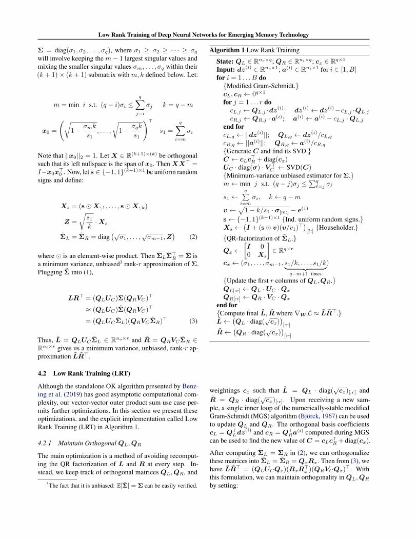
4.2 Low Rank Training (LRT)

Although the standalone OK algorithm presented by Benz-ing et al. (2019) has good asymptotic computational com-plexity, our vector-vector outer product sum use case per-mits further optimizations. In this section we present theseoptimizations, and the explicit implementation called LowRank Training (LRT) in Algorithm 1.

4.2.1 Maintain OrthogonalQL,QR

The main optimization is a method of avoiding recomput-ing the QR factorization of L and R at every step. In-stead, we keep track of orthogonal matrices QL,QR, and

3The fact that it is unbiased: E[Σ] = Σ can be easily verified.

Algorithm 1 Low Rank Training

State: QL ∈ Rno×q;QR ∈ Rni×q; cx ∈ Rq×1

Input: dz(i) ∈ Rno×1; a(i) ∈ Rni×1 for i ∈ [1, B]for i = 1 . . . B do{Modified Gram-Schmidt.}cL, cR ← 0q×1

for j = 1 . . . r docL,j ← QL,j ·dz(i); dz(i) ← dz(i)−cL,j ·QL,j

cR,j ← QR,j · a(i); a(i) ← a(i) − cL,j ·QL,j

end forcL,q ← ||dz(i)||; QL,q ← dz(i)/cL,q

cR,q ← ||a(i)||; QR,q ← a(i)/cR,q

{Generate C and find its SVD.}C ← cLc

>R + diag(cx)

UC · diag(σ) · V >C ← SVD(C){Minimum-variance unbiased estimator for Σ.}m← min j s.t. (q − j)σj ≤

∑q`=j σ`

s1 ←q∑

i=m

σi, k ← q −m

v ←√

1− k/s1 · σ[m:] − e(1)

s← {−1, 1}(k+1)×1 {Ind. uniform random signs.}Xs ←

(I + (s� v)(v/v1)>

)[2:]{Householder.}

{QR-factorization of ΣL.}

Qx ←[I 00 Xs

]∈ Rq×r

cx ← (σ1, . . . , σm−1, s1/k, . . . , s1/k︸︷︷︸q−m+1 times

)

{Update the first r columns ofQL,QR.}QL[:r] ← QL ·UC ·Qx

QR[:r] ← QR · VC ·Qx

end for{Compute final L, R where∇WL ≈ LR>.}L←

(QL · diag(

√cx))[:r]

R←(QR · diag(

√cx))[:r]

weightings cx such that L = QL · diag(√cx)[:r] and

R = QR · diag(√cx)[:r]. Upon receiving a new sam-

ple, a single inner loop of the numerically-stable modifiedGram-Schmidt (MGS) algorithm (Bjorck, 1967) can be usedto update QL and QR. The orthogonal basis coefficientscL = Q>Ldz

(i) and cR = Q>Ra(i) computed during MGS

can be used to find the new value ofC = cLc>R + diag(cx).

After computing ΣL = ΣR in (2), we can orthogonalizethese matrices into ΣL = ΣR = QxRx. Then from (3), wehave LR> = (QLUCQx)(RxR

>x )(QRVCQx)>. With

this formulation, we can maintain orthogonality inQL,QR

by setting:


QL ← QLUCQx

QR ← QRVCQx

cx ← diag(RxR>x )

These matrix multiplies require O((ni + no)q2) multipli-cations, so this optimization does not improve asymptoticcomplexity bounds. This optimization may nonetheless bepractically significant since matrix multiplies are easy toparallelize and would typically not be the bottleneck of thecomputation compared to Gram-Schmidt. The next sec-tion discusses how to orthogonalize ΣL efficiently and why(RxR

>x ) is diagonal.

4.2.2 Orthogonalization of ΣL

Orthogonalization of ΣL is relatively straightforward. From(2), the columns of ΣL are orthogonal sinceZ is orthogonal.However, they do not have unit norm. We can thereforepull out the norm into a separate diagonal matrixRx withdiagonal elements

√cx:

Qx =

[Im−1 0

0 Xs

]√cx = (

√σ1, . . . ,

√σm−1,

√s1/k︸︷︷︸

q−m+1 times

)

4.2.3 Finding Orthonormal BasisX

We generatedX by finding an orthonormal basis that wasorthogonal to a vector x0 so that we could have XX> =I − x0x

>0 . An efficient method of producing this basis is

through Householder matrices (x0,X) = I−2 vv>/||v||2where v = x0 − e(1) and (x0,X) is a k + 1 × k + 1matrix with first column x0 and remaining columns X(Householder, 1958; user1551, 2013).

4.2.4 Efficiency Comparisons to Standard Approach

The OK/LRT methods require O((ni + no + q)q2) opera-tions per sample and O(ninoq) operations after collectingB samples, giving an amortized cost ofO((ni+no+q)q2+ninoq/B) operations per sample. Meanwhile, a standardapproach expands the Kronecker sum at each sample, cost-ing O(nino) operations per sample. If q � B,ni, no thenthe low rank method is superior to minibatch SGD in bothmemory and computational cost.

4.2.5 LRT Variants

In this paper, we compare two variants of the LRT algorithm.The first one, biased LRT, is a version that compresses the

q-rank representation to rank r by taking the top r singularvalues of the SVD with no mixing. The second one, unbi-ased LRT, is a version that follows the OK algorithm andincludes mixing for minimum variance, unbiased estimatesas discussed in Section 4.1.2. While the unbiased versiondoes not add much computational complexity, it does re-quire access to random bits and introduces more varianceinto the gradient estimates. These drawbacks must be tradedoff with the benefits of having an unbiased estimator.

5 CONVEX CONVERGENCE

LRT introduces variance into the gradient estimates, so herewe analyze the implications for online convex convergence.We analyze the case of strongly convex loss landscapesf t(wt) for flattened weight vector wt and online samplet. In Appendix A, we show that with inverse squarerootlearning rate, when the loss landscape Hessians satisfy 0 ≺cI � ∇2f t(wt) and under constraint (4) for the size ofgradient errors εt, where w∗ is the optimal offline weightvector, the online regret (5) is sublinear in the number ofonline steps T . We can approximate ||ε|| and show thatconvex convergence is likely when (6) is satisfied for biasedLRT, or when (7) is satisfied for unbiased LRT.

||εt|| ≤ c

2||wt −w∗|| (4)

R(T ) =

T∑t=1

f t(wt)−T∑

t=1

f t(w∗) (5)

B∑i=1

(σ(t,i)q

)2≤ c2

4||wt −w∗||2 (6)

B∑i=1

σ(t,i)r σ(t,i)

q ≤ c2

8||wt −w∗||2 (7)

Equations (6, 7) suggest conditions under which fast conver-gence may be more or less likely and also point to methodsfor improving convergence. We discuss these in more detailin Appendix A.3.

5.1 Convergence Experiments

We validate (4) with several linear regression experimentson a static input batch X ∈ R1024×100 and target Yt ∈R256×100. In Figure 5(a), Gaussian noise at differentstrengths (represented by different colors) is added to thetrue batch gradients at each update step. Notice that con-vergence slows significantly to the right of the dashed lines,which is the region where (4) no longer holds4.

4As discussed in Appendix A.1, B < ni, so we substitute cin c/2||wt −w∗|| with the minimum non-zero Eigenvalue of theHessian c when plotting the RHS of (4).


10 2 100 102 104 106 108 1010 1012

Gradient Error Variance

10 3

10 2

10 1

100

101

102

Loss

(a) True gradients with artificial noise

104 106 108 1010 1012

Gradient Error Variance

10 1

100

101

102

103

Loss

bLRT(lr=1.0e-05) bLRT(lr=1.0e-04)bLRT(lr=1.0e-03) uLRT(lr=1.0e-05) uLRT(lr=1.0e-04) uLRT(lr=1.0e-03)

(b) Biased (bLRT) and unbiased (uLRT) gradients over learning rates

Figure 5. In both plots, the solid line with markers plots the loss vs. gradient error variance (LHS of (4)) across 50 steps of SGD forseveral different setups. The left dashed line represents the RHS of (4) and the right dashed line is the RHS with C instead of c.

In Figure 5(b), we validate Equations (4, 6, 7) by testingthe biased and unbiased LRT cases with rank r = 10. Inthese particular experiments, unbiased LRT adds too muchvariance, causing it to operate to the right of the dashedlines. However, both biased and unbiased LRT can be seento reduce their variance as training progresses. In the caseof biased LRT, it is able to continue training as it tracks theright dashed line.

6 IMPLEMENTATION DETAILS

Quantization. The NN is quantized in both the forward andbackward directions with uniform power-of-2 quantization,where the clipping ranges are fixed at the start of training5.Weights are quantized to 8 bits between -1 and 1, biases to16 bits between -8 and 8, activations to 8 bits between 0and 2, and gradients to 8 bits between -1 and 1. Both theweights W and weight updates ∆W are quantized to thesame LSB so that weights cannot be used for accumulationbeyond the fixed quantization dynamic range. This is incontrast to using high bitwidth (Zhou et al., 2016; Banneret al., 2018) or floating point accumulators. See AppendixC for more details on quantization.

Gradient Max-Norming. State-of-the-art methods in train-ing, such as Adam (Kingma & Ba, 2014), use auxiliarymemory per parameter to normalize the gradients. Unfor-tunately, we lack the memory budget to support these ad-ditional variables, especially if they must be updated everysample6. Instead, we propose dividing each gradient tensor

5Future work might look into how to change these clippingranges, but this is beyond the scope of this paper.

6LRT could potentially approximate Adam. LRT on

by the maximum absolute value of its elements. This stabi-lizes the range of gradients across samples. See AppendixD for more details on gradient max-norming. In the exper-iments, we refer to this method as “max-norm” (opposite“no-norm”).

Streaming Batch Normalization. Batch normalization(Ioffe & Szegedy, 2015) is a powerful technique for im-proving training performance which has been suggestedto work by smoothing the loss landscape (Santurkar et al.,2018). We hypothesize that this may be especially helpfulwhen parameters are quantized as in our case. However, inthe online setting, we receive samples one-at-a-time ratherthan in batches. We therefore propose a streaming batchnorm that uses moving average statistics rather than batchstatistics as described in detail in Appendix E.

7 EXPERIMENTS

7.1 Adaptation Experiments

To test the effectiveness of LRT, experiments are performedon a representative CNN with four 3× 3 convolution layersand two fully-connected layers. We generate “offline” and“online” datasets based on MNIST (see Section F), includingone in which the statistical distribution shifts every 10kimages. We then optimize the hyperparameters of both anonline SGD and rank-4 LRT model for fair comparison (seeAppendix G). To see the importance of different training

a2,dz2,a,dz allows for a low-rank approximation of the vari-ance of the gradients, however, this is unlikely to work well be-cause of numerical stability (e.g., estimated variances might benegative).


0.90

0.92

0.94

0.96

0.98

1.00

Accu

racy

Inference Bias-Only SGD/No-Norm LRT/No-Norm LRT/Max-Norm

100 101 102 103 104 105

Sample

102

105

Max

# W

rites

(a) Original Dataset

0.4

0.6

0.8

1.0

Accu

racy


CDSTBGWN

0 20000 40000 60000 80000 100000Sample

103

107

Max

# W

rites

(b) Distribution Shifts

0.2

0.4

0.6

0.8

1.0

Accu

racy


100 101 102 103 104 105

Sample

102

105

Max

# W

rites

(c) Analog / Gaussian Weight Drift

0.2

0.4

0.6

0.8

1.0

Accu

racy


100 101 102 103 104 105

Sample

102

105

Max

# W

rites

(d) Digital / Bit-Flip Weight Drift

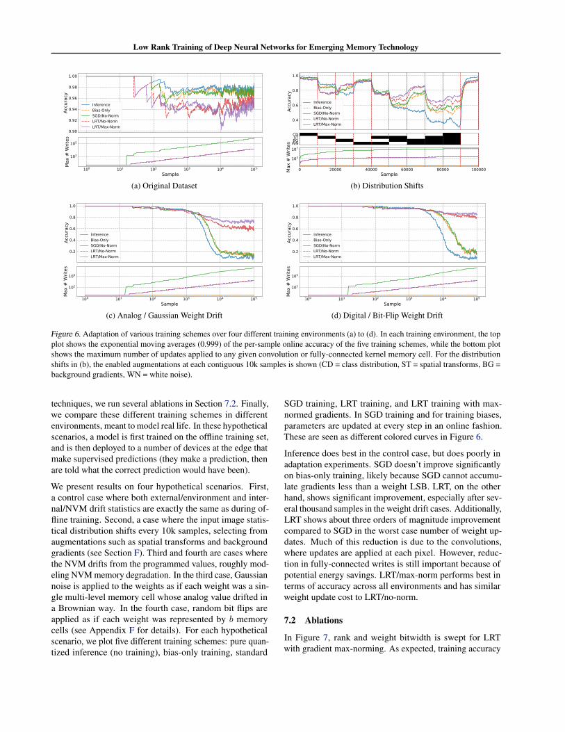
Figure 6. Adaptation of various training schemes over four different training environments (a) to (d). In each training environment, the topplot shows the exponential moving averages (0.999) of the per-sample online accuracy of the five training schemes, while the bottom plotshows the maximum number of updates applied to any given convolution or fully-connected kernel memory cell. For the distributionshifts in (b), the enabled augmentations at each contiguous 10k samples is shown (CD = class distribution, ST = spatial transforms, BG =background gradients, WN = white noise).

techniques, we run several ablations in Section 7.2. Finally,we compare these different training schemes in differentenvironments, meant to model real life. In these hypotheticalscenarios, a model is first trained on the offline training set,and is then deployed to a number of devices at the edge thatmake supervised predictions (they make a prediction, thenare told what the correct prediction would have been).

We present results on four hypothetical scenarios. First,a control case where both external/environment and inter-nal/NVM drift statistics are exactly the same as during of-fline training. Second, a case where the input image statis-tical distribution shifts every 10k samples, selecting fromaugmentations such as spatial transforms and backgroundgradients (see Section F). Third and fourth are cases wherethe NVM drifts from the programmed values, roughly mod-eling NVM memory degradation. In the third case, Gaussiannoise is applied to the weights as if each weight was a sin-gle multi-level memory cell whose analog value drifted ina Brownian way. In the fourth case, random bit flips areapplied as if each weight was represented by b memorycells (see Appendix F for details). For each hypotheticalscenario, we plot five different training schemes: pure quan-tized inference (no training), bias-only training, standard

SGD training, LRT training, and LRT training with max-normed gradients. In SGD training and for training biases,parameters are updated at every step in an online fashion.These are seen as different colored curves in Figure 6.

Inference does best in the control case, but does poorly inadaptation experiments. SGD doesn’t improve significantlyon bias-only training, likely because SGD cannot accumu-late gradients less than a weight LSB. LRT, on the otherhand, shows significant improvement, especially after sev-eral thousand samples in the weight drift cases. Additionally,LRT shows about three orders of magnitude improvementcompared to SGD in the worst case number of weight up-dates. Much of this reduction is due to the convolutions,where updates are applied at each pixel. However, reduc-tion in fully-connected writes is still important because ofpotential energy savings. LRT/max-norm performs best interms of accuracy across all environments and has similarweight update cost to LRT/no-norm.

7.2 Ablations

In Figure 7, rank and weight bitwidth is swept for LRTwith gradient max-norming. As expected, training accuracy


Table 1. Accuracy recovery beyond inference (%, mean with standard deviation from 5 random seeds) between different algorithms (allwith max-norm; effective batch size B = 100 if applicable), tested at different ranks (r), and learning rates (η). Optimal learning rates arebolded.

η 0.003 0.010 0.030 0.100 0.300Algorithm r

SGD - +0.3± 0.2 +0.3± 0.2 +0.3± 0.2 +0.9 ± 0.2 −3.9± 0.8UORO 1 +0.4 ± 0.2 +0.3± 0.4 −1.8± 0.9 −7.6± 1.6 −31.7± 1.6Biased LRT 1 +1.9± 0.2 +5.8 ± 1.0 −3.4± 1.0 −19.4± 0.9 −40.7± 1.1

2 +1.4± 0.4 +6.5 ± 0.7 +6.3± 0.6 −5.2± 0.9 −36.3± 0.94 +1.3± 0.4 +6.5 ± 0.7 +5.2± 0.8 −3.3± 1.0 −33.8± 0.88 +1.4± 0.3 +5.6 ± 0.8 +4.3± 0.9 −2.4± 1.0 −32.8± 0.9

Unbiased LRT 1 +0.3 ± 0.2 +0.3± 0.2 −0.7± 0.4 −2.7± 1.7 −26.5± 2.62 +0.3± 0.2 +0.4± 0.3 −0.1± 0.4 +1.3 ± 0.9 −12.9± 1.14 +0.4± 0.2 +0.6± 0.2 +1.9± 0.3 +8.0 ± 1.1 −5.1± 1.18 +0.4± 0.2 +1.1± 0.2 +3.3± 0.7 +4.8 ± 1.5 −15.8± 1.7

Table 2. Importance of unbiased SVD. Accuracy is calculated from the last 500 samples of 10k samples trained from scratch. Mean andunbiased standard deviation are calculated from five runs of different random seeds.

Conv LRT FC LRT Accuracy (no-norm) Accuracy (max-norm)Biased Biased 79.7%± 1.1% 82.7%± 1.3%Biased Unbiased 83.0%± 0.9% 82.4%± 1.2%Unbiased Biased 77.7%± 1.5% 84.6%± 2.0%Unbiased Unbiased 81.0%± 0.9% 83.6%± 2.5%

improves with both higher LRT rank and bitwidth. In denseNVM applications, higher bitwidths may be achievable,allowing for corresponding reductions in the LRT rank andtherefore, reductions in the auxiliary memory requirements.

1 2 3 4 5 6 7 8 9 10LRT/Max-Norm Rank

1

2

3

4

5

6

7

8

Wei

ght B

itwid

th

12%

12%

40%

45%

51%

55%

56%

53%

12%

9%

42%

50%

58%

64%

65%

59%

13%

31%

40%

55%

61%

64%

68%

67%

13%

26%

44%

59%

62%

69%

72%

69%

12%

10%

43%

54%

68%

74%

74%

72%

12%

12%

45%

63%

69%

74%

79%

75%

14%

9%

49%

63%

75%

76%

75%

74%

13%

9%

52%

64%

76%

74%

79%

76%

14%

9%

52%

70%

77%

77%

79%

80%

12%

10%

49%

70%

78%

77%

76%

76%

0.0

0.2

0.4

0.6

0.8

1.0

Accu

racy

(Las

t 500

of 2

k)

Figure 7. Accuracy across a variety of LRT ranks and weightbitwidths, showing the expected trends of increasing accuracywith rank and bitwidth. Accuracy is calculated by averaging theaccuracy on the last 500 samples from a 2k portion of the trainingdata. For bitwidths of 1 and 2, mid-rise quantization is used (e.g.,1 bit quantizes values to -0.5 and 0.5 instead of -1 and 0).

In Table 2, biased (zero-variance) and unbiased (low-variance) versions of LRT are compared. Accuracy improve-

ments are generally seen moving from biased to unbiasedLRT although the pattern differs between the no-norm andmax-norm cases. In the no-norm case, a significant improve-ment is seen favoring unbiased LRT for fully-connectedlayers. In the max-norm case, the choice of biased or un-biased LRT has only a minor impact on accuracy. It mightbe expected that as the number of accumulated samples fora given batch increases, lower variance would be increas-ingly important at the expense of bias. For our network, thisimplies convolutions, which receive updates at every pixelof an output feature map, would preferentially have biasedLRT, while the fully-connected layer would preferentiallybe unbiased. This hypothesis is supported by the no-normexperiments, but not by the max-norm experiments.

In Table 3, several ablations are performed on LRT withmax-norm. Most notably, weight training is found to be ex-tremely important for accuracy as bias-only training showsa ≈ 15 − 30% accuracy hit depending on whether max-norming is used. Streaming batch norm is also found to bequite helpful, especially in the no-norm case.

Now, we explain the κth ablation. In Section 4.1.1, wefound the SVD of a small matrix C and its singular val-ues σ1, . . . , σq. This allows us to easily find the conditionnumber of C as κ(C) = σ1/σq . We suspect high conditionnumbers provide relatively useless update information akinto noise, especially in the presence of L,R quantization.


Table 3. Miscellaneous selected ablations. Accuracy is calculated from the last 500 samples of 10k samples trained from scratch. Meanand unbiased standard deviation are calculated from five runs of different random seeds.

Modified Condition Accuracy (no-norm) Accuracy (max-norm)baseline (no modifications) 80.2%± 1.0% 83.0%± 1.1%bias-only training 51.8%± 3.2% 68.6%± 1.4%no streaming batch norm 68.2%± 1.9% 81.8%± 1.3%no bias training 81.3%± 1.0% 83.0%± 1.4%κth = 108 instead of 100 79.8%± 1.4% 84.2%± 1.4%

Therefore, we prefer not to update L,R on samples whosecondition number exceeds threshold κth. We can avoid per-forming an actual SVD (saving computation) by noting thatC is often nearly diagonal, leading to the approximationκ(C) ≈ C1,1/Cq,q . Empirically, this rough heuristic workswell to reduce computation load while having minor impacton accuracy. In Table 3, κth = 108 does not appear to ubiq-uitously improve on the default κth = 100, despite being≈ 2× slower to compute.

7.3 Transfer Learning and Algorithm Comparisons

To test the broader applicability of low rank training tech-niques, we run several experiments on ImageNet withResNet-34 (Deng et al., 2009; He et al., 2016), a poten-tially realistic target for dense NVM inference on-chip. ForImageNet-size images, updating the low-rank approxima-tion at each pixel quickly becomes infeasible, both becauseof the single-threaded nature of the algorithm, and becauseof the increased variance of the estimate at larger batchsizes. Instead, we focus on training the final layer weights(1000 × 512). ResNet-34 weights are initialized to thosefrom Paszke et al. (2017) and the convolution layers areused to generate feature vectors for 10k ImageNet trainingimages7, which are quantized and fed to a one-layer quan-tized8 neural network. To speed up experiments, the layerweights are initialized to the pretrain weights, modulated byrandom noise that causes inference top-1 accuracy to fall to52.7% ± 0.9%. In Table 1, we see that the unbiased LRThas the strongest recovery accuracies, although biased LRTalso does quite well. The high-variance UORO and trueSGD have weak or non-existent recoveries.

8 CONCLUSION

We demonstrated the potential for LRT to solve the majorchallenges facing online training on NVM-based edge de-vices: low write density and low auxiliary memory. LRT is a

7The decision to use training data is deliberate, however exper-iments on out-of-sample images, such as Recht et al. (2019) showsimilar behavior.

8Quantization ranges are chosen to optimize accuracy and aredifferent from those in Section 7.1.

computationally-efficient, memory-light algorithm capableof decoupling batch size from auxiliary memory, allowinglarger effective batch sizes, and consequently lower writedensities. Additionally, we noted that LRT may allow fortraining under severe weight quantization constraints as rudi-mentary gradient accumulations are handled by the L,Rmatrices, which can have high bitwidths (as opposed toSGD, which may squash small gradients to 0).

We found expressions for when LRT might have better con-vergence properties. Across a variety of online adaptationproblems and a large-scale transfer learning demonstration,LRT was shown to match or exceed the performance ofSGD while using a small fraction of the number of updates.

Finally, we conclude with speculations about more generalapplications of the LRT technique. Auxiliary memory mini-mization may be analogous to communication minimizationin training strategies such as federated learning, where gra-dient compression is important. Therefore, LRT could be avaluable tool for local training of networks of devices thatcommunicate training information to each other, withoutthe use of a central server.


REFERENCES

Aji, A. F. and Heafield, K. Sparse communica-tion for distributed gradient descent. arXiv preprintarXiv:1704.05021, 2017.

Ambrogio, S., Narayanan, P., Tsai, H., Shelby, R. M., Boy-bat, I., di Nolfo, C., Sidler, S., Giordano, M., Bodini,M., Farinha, N. C. P., Killeen, B., Cheng, C., Jaoudi,Y., and Burr, G. W. Equivalent-accuracy acceleratedneural-network training using analogue memory. Nature,558(7708):60–67, June 2018. ISSN 1476-4687. doi:10.1038/s41586-018-0180-5.

Banner, R., Hubara, I., Hoffer, E., and Soudry, D. Scal-able methods for 8-bit training of neural networks. InAdvances in Neural Information Processing Systems, pp.5145–5153, 2018.

Bengio, Y., Leonard, N., and Courville, A. Estimating orpropagating gradients through stochastic neurons for con-ditional computation. arXiv preprint arXiv:1308.3432,2013.

Benzing, F., Gauy, M. M., Mujika, A., Martinsson, A.,and Steger, A. Optimal Kronecker-sum approxima-tion of real time recurrent learning. In Chaudhuri, K.and Salakhutdinov, R. (eds.), Proceedings of the 36thInternational Conference on Machine Learning, vol-ume 97 of Proceedings of Machine Learning Research,pp. 604–613, Long Beach, California, USA, 09–15 Jun2019. PMLR. URL http://proceedings.mlr.press/v97/benzing19a.html.

Bjorck, A. Solving linear least squares problems by gram-schmidt orthogonalization. BIT Numerical Mathematics,7(1):1–21, 1967.

Boyd, S. and Vandenberghe, L. Convex optimization. Cam-bridge university press, 2004.

Chou, C., Lin, Z., Tseng, P., Li, C., Chang, C., Chen, W.,Chih, Y., and Chang, T. J. An N40 256K×44 embeddedRRAM macro with SL-precharge SA and low-voltagecurrent limiter to improve read and write performance. In2018 IEEE International Solid - State Circuits Conference- (ISSCC), pp. 478–480, February 2018. doi: 10.1109/ISSCC.2018.8310392.

Cline, A. K. and Dhillon, I. S. Computation of the singularvalue decomposition, 2006.

Deng, J., Dong, W., Socher, R., Li, L.-J., Li, K., and Fei-Fei, L. ImageNet: A Large-Scale Hierarchical ImageDatabase. In CVPR09, 2009.

Ernestus, M. Elastic transformation of an im-age in python. https://gist.github.com/erniejunior/601cdf56d2b424757de5, 2016.

Gokmen, T. and Vlasov, Y. Acceleration of Deep NeuralNetwork Training with Resistive Cross-Point Devices.Frontiers in Neuroscience, 10, July 2016. ISSN 1662-453X. doi: 10.3389/fnins.2016.00333.

Gonugondla, S. K., Kang, M., and Shanbhag, N. R. AVariation-Tolerant In-Memory Machine Learning Clas-sifier via On-Chip Training. IEEE Journal of Solid-State Circuits, 53(11):3163–3173, November 2018. doi:10.1109/JSSC.2018.2867275.

Goyal, P., Dollar, P., Girshick, R., Noordhuis, P.,Wesolowski, L., Kyrola, A., Tulloch, A., Jia, Y., andHe, K. Accurate, large minibatch sgd: Training imagenetin 1 hour. arXiv preprint arXiv:1706.02677, 2017.

Grossi, A., Vianello, E., Sabry, M. M., Barlas, M., Grenouil-let, L., Coignus, J., Beigne, E., Wu, T., Le, B. Q., Woot-ters, M. K., Zambelli, C., Nowak, E., and Mitra, S. Re-sistive ram endurance: Array-level characterization andcorrection techniques targeting deep learning applications.IEEE Transactions on Electron Devices, 66(3):1281–1288, March 2019. doi: 10.1109/TED.2019.2894387.

Haykin, S. Adaptive filter theory, ser. always learning, 2014.

He, K., Zhang, X., Ren, S., and Sun, J. Delving deepinto rectifiers: Surpassing human-level performance onimagenet classification. In Proceedings of the IEEE inter-national conference on computer vision, pp. 1026–1034,2015.

He, K., Zhang, X., Ren, S., and Sun, J. Deep residual learn-ing for image recognition. In Proceedings of the IEEEconference on computer vision and pattern recognition,pp. 770–778, 2016.

Householder, A. S. Unitary triangularization of a nonsym-metric matrix. Journal of the ACM (JACM), 5(4):339–342, 1958.

Ioffe, S. and Szegedy, C. Batch normalization: Acceleratingdeep network training by reducing internal covariate shift.arXiv preprint arXiv:1502.03167, 2015.

Kingma, D. P. and Ba, J. Adam: A method for stochasticoptimization. arXiv preprint arXiv:1412.6980, 2014.

Konecny, J., McMahan, H. B., Ramage, D., and Richtarik,P. Federated optimization: Distributed machine learningfor on-device intelligence. CoRR, abs/1610.02527, 2016.URL http://arxiv.org/abs/1610.02527.

LeCun, Y., Bottou, L., Bengio, Y., Haffner, P., et al.Gradient-based learning applied to document recognition.Proceedings of the IEEE, 86(11):2278–2324, 1998.

http://proceedings.mlr.press/v97/benzing19a.html

http://proceedings.mlr.press/v97/benzing19a.html

https://gist.github.com/erniejunior/601cdf56d2b424757de5

https://gist.github.com/erniejunior/601cdf56d2b424757de5

http://arxiv.org/abs/1610.02527


Lin, Y., Han, S., Mao, H., Wang, Y., and Dally, W. J.Deep gradient compression: Reducing the communica-tion bandwidth for distributed training. arXiv preprintarXiv:1712.01887, 2017.

Ling, F., Manolakis, D., and Proakis, J. A recursive modi-fied gram-schmidt algorithm for least-squares estimation.IEEE transactions on acoustics, speech, and signal pro-cessing, 34(4):829–836, 1986.

Mujika, A., Meier, F., and Steger, A. Approximating real-time recurrent learning with random kronecker factors.In Advances in Neural Information Processing Systems,pp. 6594–6603, 2018.

Paszke, A., Gross, S., Chintala, S., Chanan, G., Yang, E.,DeVito, Z., Lin, Z., Desmaison, A., Antiga, L., and Lerer,A. Automatic differentiation in pytorch. 2017.

Qi, H., Brown, M., and Lowe, D. G. Low-Shot Learningwith Imprinted Weights. In 2018 IEEE/CVF Conferenceon Computer Vision and Pattern Recognition, pp. 5822–5830, Salt Lake City, UT, June 2018. IEEE. ISBN 978-1-5386-6420-9. doi: 10.1109/CVPR.2018.00610.

Recht, B., Roelofs, R., Schmidt, L., and Shankar, V. Do im-agenet classifiers generalize to imagenet? arXiv preprintarXiv:1902.10811, 2019.

Ren, J. S. and Xu, L. On vectorization of deep convolutionalneural networks for vision tasks. In Twenty-Ninth AAAIConference on Artificial Intelligence, 2015.

Santurkar, S., Tsipras, D., Ilyas, A., and Madry, A. Howdoes batch normalization help optimization? In Ad-vances in Neural Information Processing Systems, pp.2483–2493, 2018.

Simard, P. Y., Steinkraus, D., and Platt, J. Best prac-tices for convolutional neural networks appliedto visual document analysis. Institute of Electri-cal and Electronics Engineers, Inc., August 2003.URL https://www.microsoft.com/en-us/research/publication/best-practices-for-convolutional-neural-networks-applied-to-visual-document-analysis/.

Soudry, D., Castro, D. D., Gal, A., Kolodny, A., and Kvatin-sky, S. Memristor-Based Multilayer Neural NetworksWith Online Gradient Descent Training. IEEE Transac-tions on Neural Networks and Learning Systems, 26(10):2408–2421, October 2015. doi: 10.1109/TNNLS.2014.2383395.

Tallec, C. and Ollivier, Y. Unbiased online recurrent opti-mization. arXiv preprint arXiv:1702.05043, 2017.

TSMC. 40nm Technology - Taiwan Semicon-ductor Manufacturing Company Limited, 2019.URL https://www.tsmc.com/english/dedicatedFoundry/technology/40nm.htm.

user1551. Rotation matrix in arbitrary di-mension to align vector. MathematicsStack Exchange, 2013. URL https://math.stackexchange.com/q/525587.URL:https://math.stackexchange.com/q/525587 (version:2013-10-14).

Williams, R. J. and Zipser, D. A learning algorithm for con-tinually running fully recurrent neural networks. Neuralcomputation, 1(2):270–280, 1989.

Wu, T. F., Le, B. Q., Radway, R., Bartolo, A., Hwang,W., Jeong, S., Li, H., Tandon, P., Vianello, E., Vivet, P.,Nowak, E., Wootters, M. K., Wong, H. . P., Aly, M. M. S.,Beigne, E., and Mitra, S. 14.3 a 43pj/cycle non-volatilemicrocontroller with 4.7us shutdown/wake-up integrating2.3-bit/cell resistive ram and resilience techniques. In2019 IEEE International Solid- State Circuits Conference- (ISSCC), pp. 226–228, Feb 2019. doi: 10.1109/ISSCC.2019.8662402.

Yu, S. Neuro-inspired computing with emerging nonvolatilememorys. Proceedings of the IEEE, 106(2):260–285,2018.

Yu, S., Li, Z., Chen, P., Wu, H., Gao, B., Wang, D., Wu, W.,and Qian, H. Binary neural network with 16 Mb RRAMmacro chip for classification and online training. In 2016IEEE International Electron Devices Meeting (IEDM),pp. 16.2.1–16.2.4, December 2016. doi: 10.1109/IEDM.2016.7838429.

Zamanidoost, E., Bayat, F. M., Strukov, D., and Kataeva,I. Manhattan rule training for memristive crossbar cir-cuit pattern classifiers. In 2015 IEEE 9th InternationalSymposium on Intelligent Signal Processing (WISP) Pro-ceedings, pp. 1–6, May 2015. doi: 10.1109/WISP.2015.7139171.

Zhang, J., Wang, Z., and Verma, N. In-Memory Compu-tation of a Machine-Learning Classifier in a Standard6T SRAM Array. IEEE Journal of Solid-State Circuits,52(4):915–924, April 2017. ISSN 0018-9200. doi:10.1109/JSSC.2016.2642198.

Zhou, S., Wu, Y., Ni, Z., Zhou, X., Wen, H., and Zou, Y.Dorefa-net: Training low bitwidth convolutional neuralnetworks with low bitwidth gradients. arXiv preprintarXiv:1606.06160, 2016.

Zinkevich, M. Online convex programming and generalizedinfinitesimal gradient ascent. In Proceedings of the 20th

https://www.microsoft.com/en-us/research/publication/best-practices-for-convolutional-neural-networks-applied-to-visual-document-analysis/




https://www.tsmc.com/english/dedicatedFoundry/technology/40nm.htm

https://www.tsmc.com/english/dedicatedFoundry/technology/40nm.htm

https://math.stackexchange.com/q/525587

https://math.stackexchange.com/q/525587


International Conference on Machine Learning (ICML-03), pp. 928–936, 2003.


A CONVEX CONVERGENCE

In this section we will attempt to bound the regret (definedbelow) of an SGD algorithm using noisy LRT estimatesg = g + ε in the convex setting, where g are the truegradients and ε are the errors introduced by the low rankLRT approximation. Here, g is a vector of size N andcan be thought of as a flattened/concatenated version of thegradient tensors (e.g., N = ni · no).

Our proof follows the proof in Zinkevich (2003). We de-fine F as the convex feasible set (valid settings for ourweight tensors) and assume that F is bounded with D =maxw,v∈F||w − v|| being the maximum distance betweentwo elements of F. Further, assume a batch t of B sam-ples out of T total batches corresponds to a loss landscapef t(wt) that is strongly convex in weight parameters wt,so there are positive constants C ≥ c > 0 such that cI �∇2f t(wt) � CI for all t (Boyd & Vandenberghe, 2004).We define regret as R(T ) =

∑Tt=1 f

t(wt)−∑T

t=1 ft(w∗)

where w∗ = argminw∑T

t=1 ft(w) (i.e., it is an optimal

offline minimizer of f1, · · · , fT ).

The gradients seen during SGD are gt = ∇f t(wt)and we assume they are bounded by G =maxw∈F,t∈[1,T ]||∇f t(w)||. We also assume errorsare bounded by E = maxt∈[1,T ]||εt||. Therefore,maxt∈[1,T ]||gt|| ≤ maxt∈[1,T ]||gt|| + ||εt|| ≤ G + E bythe triangle inequality.

Theorem 1. Assume LRT-based SGD is applied with learn-ing rate ηt = 1/

√t. Then, under the additional constraint

gt · (wt−w∗)− c2 ||w

t−w∗||22 ≤ gt · (wt−w∗), we havesublinear regret:

R(T ) ≤ D2

2

√T + (G+ E)2

(√T − 1/2

)

Proof. From strong convexity cI � ∇2f t(wt) � CI forall t,

f t(w)+gt ·(v−w)+c

2||v−w||22 ≤ f t(v) for all v (8)

In particular, if we consider v = w∗ and rearrange,

f t(w)− f t(w∗) ≤ gt · (w −w∗)− c

2||w −w∗||22

f t(w)− f t(w∗) ≤ gt · (wt −w∗) (9)

Consider a gradient update wt+1 = PF(wt − ηtgt), wherePF projects the update back to F. Then,

||wt+1 −w∗||22 = ||P (wt − ηtgt)−w∗||22≤ ||wt − ηtgt −w∗||22= ||wt −w∗||22 − 2ηt(w

t −w∗) · gt+η2t ||gt||22≤ ||wt −w∗||22 − 2ηt(w

t −w∗) · gt+η2t (G+ E)2

gt · (wt −w∗) ≤ 1

2ηt

(||wt −w∗||22 − ||wt+1 −w∗||22

)+

ηt2

(G+ E)2 (10)

From (9, 10),

f t(wt)− f t(w∗) ≤ 1

2ηt

(||wt −w∗||22 − ||wt+1 −w∗||22

)+

ηt2

(G+ E)2 (11)

We now bound the regret:

R(T ) =

T∑t=1

[f t(wt)− f t(w∗)

]≤

T∑t=1

[1

2ηt

(||wt −w∗||22 − ||wt+1 −w∗||22

)+

ηt2

(G+ E)2]

=||w1 −w∗||22

2η1− ||w

T+1 −w∗||222ηT

+

1

2

T∑t=2

(1

ηt− 1

ηt−1

)||wt −w∗||22 +

(G+ E)2

2

T∑t=1

ηt

≤ ||w1 −w∗||22

2η1+

1

2

T∑t=2

(1

ηt− 1

ηt−1

)||wt −w∗||22+

(G+ E)2

2

T∑t=1

ηt

≤ D2

2η1+

1

2

T∑t=2

(1

ηt− 1

ηt−1

)D2 +

(G+ E)2

2

T∑t=1

ηt

=D2

2ηT+

(G+ E)2

2

T∑t=1

ηt (12)

If ηt = 1/√t, then

∑Tt=1 ηt ≤ 2

√T − 1 (Zinkevich, 2003),

so from (12),


R(T ) ≤ D2

2

√T + (G+ E)2

(√T − 1/2

)(13)

This is a sublinear regret and therefore, average regretR(T )/T is bounded above by 0 in the limit as T → ∞.To achieve this result, we constrained gt · (wt − w∗) −c2 ||w

t −w∗||22 ≤ gt · (wt −w∗). We now examine suffi-cient conditions for this inequality to be satisfied.

gt · (wt −w∗)− c

2||wt −w∗||22 ≤ gt · (wt −w∗)

εt · (w∗ −wt) ≤ c

2||wt −w∗||22

(14)

Since εt · (w∗ − wt) ≤ ||εt|| · ||w∗ − wt|| by Cauchy-Schwarz, it is sufficient for:

||εt|| · ||w∗ −wt|| ≤ c

2||wt −w∗||22

||εt|| ≤ c

2||wt −w∗|| (15)

A.1 Considerations for Rank Deficient Hessians

In the preceding proof, we assumed c > 0. However, itis common for this to not hold. For example, in linearregression, where c = λmin(XX>) for sample inputX ∈R(ni×B) (Haykin, 2014, Chapter 4.3), if B < ni then c =0. We can modify (15) to handle this case. Let c be theminimum non-zero Eigenvalue of XX> and let w ∈ RB

represent w ∈ RN in the Eigenbasis of XX>. Then (15)becomes:

||εt|| ≤ c

2||wt − w∗|| (16)

A.2 Estimates for the LRT Error

We can estimate the LRT error ||εt|| in both the biasedand unbiased cases. For the biased, zero-variance case,we get rid of the lowest singular value (out of q singularvalues) as we see each sample. Thus, at a given sample i,the error is σ(i)

q ·Q(i)L,q ·Q

(i)R,q and the average squared error

is (1/N)σ(i)2q . We can treat this as a per-element variance.

If these smallest singular components are uncorrelated fromsample to sample, then the variances add:

σ2ε ≈

1

N

B∑i=1

(σ(i)q

)2(17)

For the unbiased, minimum-variance case, Theorem A.4from Benzing et al. (2019) states that the minimum varianceis s21/k + s2 where s1 =

∑qi=m σi, s2 =

∑qi=m σ2

i , andk,m are as defined in Section 4.1.2. Since m is chosento minimize variance, we can upper bound the variance bychoosing m = r and therefore k = 1, s1 = σr + σq, ands2 = σ2

r + σ2q . Empirically, this tends to be a good ap-

proximation. Then, the average per-element variance addedat sample i is approximately (2/N)

(σ(i)r σ

(i)q

). Assuming

errors between samples are uncorrelated, this leads to a totalvariance:

σ2ε ≈

2

N

B∑i=1

σ(i)r σ(i)

q (18)

For either case, ||ε||2 ≈ Nσ2ε . For the t-th batch and i-th

sample, we denote σ(t,i)q as the q-th singular value. For

simplicity, we focus on the biased, zero-variance case (theunbiased case is similar). From (15), an approximatelysufficient condition for sublinear-regret convergence is:

B∑i=1

(σ(t,i)q

)2≤ c2

4||wt −w∗||2 (19)

A.3 Discussion on Convergence

Equation (19) suggests that as wt → w∗, the constraintsfor achieving sublinear-regret convergence become moredifficult to maintain. However, in practice this may be highlyproblem-dependent as the σq will also tend to decrease nearoptimal solutions. To get a better sense of the behavior ofthe left-hand side of (19), suppose that:

B∑i=1

(σ(t,i)q

)2≈

B∑i=q

(σi(G

t))2

≤B∑i=1

(σi(G

t))2

= ||Gt||2F

where Gt = ∇W tf t(W t) ∈ R(no×ni) are the matrixweight W t gradients at batch t and || · ||F is a Frobeniusnorm. We therefore expect both the left (proportional to||Gt||2F ) and the right (proportional to ||wt−w∗||2) of (19)to decrease during training as wt → w∗. This behavioris in fact what is seen in Figure 5(b). If achieving conver-gence is found to be difficult, (19) provides some insight forconvergence improvement methods.

One solution is to reduce batch size B to satisfy the in-equality as necessary. This minimizes the weight updates


during more repetitive parts of training while allowing denseweight updates (possibly approaching standard SGD withsmall batch sizes) during more challenging parts of training.

Another solution is to reduce σq. One way to do this is toincrease the rank r so that the spectral energy of the updatesare spread across more singular components. There maybe alternate approaches based on conditioning the inputs toshape the distribution of singular values in a beneficial way.

A third method is to focus on c, the lower bound on curva-ture of the convex loss functions. Perhaps a technique suchas weight regularization can increase c by adding constantcurvature in all Eigen-directions of the loss function Hessian(although this may also increase the LHS of (19)). Alter-natively, perhaps low-curvature Eigen-directions are lessimportant for loss minimization, allowing us to raise the cthat we effectively care about. This latter approach requiresno particular action on our part, except the recognition thatfast convergence may only be guaranteed for high-curvaturedirections. This is exemplified in Figure 5(b), where we cansee biased LRT track the curve for C more so than c.

Finally, we note that this analysis focuses solely on the errorsintroduced by a floating-point version of LRT. Quantizationnoise can add additional error into the εt term. We expectthis to add a constant offset to the LHS of (19). For aweight LSB ∆, quantization noise has variance ∆2/12, sowe desire:

N∆2

12+

B∑i=1

(σ(t,i)q

)2≤ c2

4||wt −w∗||2 (20)

B KRONECKER SUMS IN NEURALNETWORK LAYERS

B.1 Dense Layer

A dense or fully-connected layer transforms an input a ∈Rni×1 to an intermediate z = W · a + b to an outputy = σ(z) ∈ Rno×1 where σ is a non-linear activationfunction. Gradients of the loss function with respect to theweight parameters can be found as:

∇WL = (∇zL)︸︷︷︸dz

� (∇W z)︸︷︷︸a>

= dz ⊗ a (21)

which is exactly the per-sample Kronecker sum update wesaw in linear regression. Thus, at every training sample, wecan add (dz(i) ⊗ a(i)) to our low rank estimate with LRT.

B.2 Convolutional Layer

A convolutional layer transforms an input feature mapA ∈ Rhin×win×cin to an intermediate feature map Z =

Wkern ∗ A + b ∈ Rhout×wout×cout through a 2D convo-lution ∗ with weight kernel Wkern ∈ Rcout×kh×kw×cin .Then it computes an output feature map y = σ(z) where σis a non-linear activation function.

Convolutions can be interpreted as matrix multiplicationsthrough the im2col operation which converts the inputfeature map A into a matrixAcol ∈ R(houtwout)×(khkwcin)

where the ith row is a flattened version of the sub-tensor ofa which is dotted with Wkern to produce the ith pixel of theoutput feature map (Ren & Xu, 2015). We can multiplyAcol

by a flattened version of the kernel,W ∈ Rcout×(khhwcin)

to perform the Wkern ∗ A convolution operation with amatrix multiplication. Under the matrix multiplication inter-pretation, weight gradients can be represented as:

∇WL = (∇ZcolL)︸︷︷︸

dZ>col

� (∇WZ)︸︷︷︸Acol

=

houtwout∑i=1

dZ>col,i ⊗A>col,i (22)

which is the same as houtwout Kronecker sum updates.Thus, at every output pixel j of every training sample i,we can add (dZ

(i)>col,j⊗A

(i)>col,j) to our low rank estimate with

LRT.

Note that while we already save an impressive factor ofB/q in memory when computing gradients for the denselayer, we save a much larger factor ofBhoutwout/q in mem-ory when computing gradients for the convolution layers,making the low rank training technique even more crucialhere.

However, some care must be taken when considering acti-vation memory for convolutions. For compute-constrainededge devices, image dimensions may be small and resultin minimal intermediate feature map memory requirements.However, if image dimensions grow substantially, activa-tion memory could dominate compared to weight storage.Clever dataflow strategies may provide a way to reduceintermediate activation storage even when performing back-propagation9.


𝑊ℓ

𝑏ℓ

𝛼ℓ

𝑎ℓ−1 𝑎ℓ

𝛿ℓ𝛿ℓ−1

SKS

×

×

lr

𝑄𝑤8𝑏−1 𝑡𝑜 1

𝑄𝑏16𝑏−8 𝑡𝑜 8

𝑄𝑎8𝑏0 𝑡𝑜 2

∗ × 𝑄𝑏16𝑏−8 𝑡𝑜 8 + 𝑄𝑏16𝑏

−8 𝑡𝑜 8

ReLU

𝑄𝑔8𝑏−1 𝑡𝑜 1

𝑄𝑤8𝑏−1 𝑡𝑜 1

𝑄𝑏16𝑏−8 𝑡𝑜 8

Figure 8. Signal flow graph for a forward and backward quantized convolutional or dense layer.

C HARDWARE QUANTIZATION MODEL

In a real device, operations are expected to be performedin fixed point arithmetic. Therefore, all of our trainingexperiments are conducted with quantization in the loop.Our model for quantization is shown in Figure 8. Thegreen arrows describe the forward computation. Ignor-ing quantization for a moment, we would have a` =ReLU

(α`W ` ∗ a`−1 + b`

), where ∗ can represent either

a convolution or a matrix multiply depending on the layertype and α` is the closest power-of-2 to He initialization(He et al., 2015). For quantization, we rely on four basicquantizers: Qw,Qb,Qa,Qg, which describe weight quan-tization, bias and intermediate accumulator quantization,activation quantization, and gradient quantization, respec-tively. All quantizers use fixed clipping ranges as depictedand quantize uniformly within those ranges to the specifiedbitwidths.

In the backward pass, follow the orange arrows from δ`.Backpropagation follows standard backpropagation rulesincluding using the straight-through estimator (Bengio et al.,2013) for quantizer gradients. However, because we wantto perform training on edge devices, these gradients mustthemselves be quantized. The first place this happens is afterpassing backward through the ReLU derivitive. The othertwo places are before feeding back into the network param-

9For example, one could compute just a sliding window ofrows of every feature map, discarding earlier rows as later rowsare computed, resulting in a square-root reduction of activationmemory. To incorporate backpropagation, compute the forwardpass once fully, then compute the forward pass again, as well asthe backward pass using the sliding window approach in bothdirections.

etersW `, b`, so thatW `, b` cannot be used to accumulatevalues smaller than their LSB. Finally, instead of deriving∆W ` from a backward pass through the ∗ operator, theLRT method is used.

LRT collects a`−1,dz` for many samples before computingthe approximate ∆W `. It accumulates information in twolow rank matrices L,R which are themselves quantizedto 16 bits with clipping ranges determined dynamically bythe max absolute value of elements in each matrix. WhileLRT accumulates for B samples, leading to a factor of Breduction in the rate of updates toW `, b` is updated at everysample. This is feasible in hardware because b` is smallenough to be stored in more expensive forms of memorythat have superior endurance and write power performance.

Because of the coarse weight LSB size, weight gradientsmay be consistently quantized to 0, preventing them fromaccumulating. To combat this, we only apply an update ifa minimum update density ρmin = 0.01 would be achieved,otherwise we continue accumulating samples in L andR,which have much higher bitwidths. When an update does fi-nally happen, the “effective batch size” will be a multiple ofB and we increase the learning rate correspondingly. In theliterature, a linear scaling rule is suggested (see Goyal et al.(2017)), however we empirically find square-root scalingworks better (see Appendix G).

D GRADIENT MAX-NORMING

Figure 9 plots the magnitude of gradients seen in a weighttensor over training steps. One apparent property of thesegradients is that they have a large dynamic range, mak-ing them difficult to quantize. Even when looking at just


Figure 9. Maximum magnitude of weight gradients versus trainingstep for standard SGD on a CNN trained on MNIST.

the spikes, they assume a wide range of magnitudes. Onepotential method of dealing with this dynamic range is toscale tensors so that their max absolute element is 1 (similarto a per-tensor AdaMax (Kingma & Ba, 2014) or RangeBatch-Norm (Banner et al., 2018) applied to gradients).Optimizers such as Adam, which normalize by gradientvariance, provide a justification for why this sort of scal-ing might work well, although they work at a per-elementrather than per-tensor level. We choose max-norming ratherthan variance-based norming because the former is easiercomputational and potentially more ammenable to quantiza-tion. However, a problem with the approach of normalizingtensors independently at each sample is that noise mightbe magnified during regions of quiet as seen in the Figure.What we therefore propose is normalization by the maxi-mum of both the current max element and a moving averageof the max element.

Explicitly, max-norm takes two parameters - a decay factorβ = 0.999 and a gradient floor ε = 10−4 and keeps twostate variables - the number of evaluations k := 0 and thecurrent maximum moving average xmv := ε. Then fora given input x, max-norm modifies its internal state andreturns xnorm:

k := k + 1

xmax := max(|x|) + ε

xmv := β · xmv + (1− β) · xmax

xmv :=xmv

1− βk

xnorm :=x

max(xmax, xmv)

E STREAMING BATCH NORMALIZATION

Standard batch normalization (Ioffe & Szegedy, 2015) nor-malizes a tensor X along some axes, then applies a trainableaffine transformation. For each sliceX of X that is normal-ized independently:

Y = γ · X − µb√σ2b + ε

+ β

where µb, σb are mean and standard deviation statistics ofa minibatch and γ, β are trainable affine transformationparameters.

In our case, we do not have the memory to hold a batchof samples at a time and must compute µb, σb in an onlinefashion. To see how this works, suppose we knew the statis-tics of each sample µi, σi for i = 1 . . . B in a batch of Bsamples. For simplicity, assume the ith sample is a vectorXi,: ∈ Rn containing elements Xi,j . Then:

µb =1

B

B∑i=1

µi (23)

σ2b =

1

B

B∑i=1

1

n

n∑j=1

X2i,j − µ2

b

=1

B

B∑i=1

(σ2i + µ2

i

)− µ2

b

6= 1

B

B∑i=1

σ2i (24)

In other words, the batch variance is not equal to the averageof the sample variances. However, if we keep track of thesum-of-square values of samples σ2

i + µ2i , then we can

compute σ2b as in (24). We keep track of two state variables:

µs, sqs which we update as µs := µs + µi and sqs :=sqs + σ2

i + µ2i for each sample i. After B samples, we

divide both state variables by B and apply (23, 24) to getthe desired batch statistics. Unfortunately, in an onlinesetting, all samples prior to the last one in a given batchwill only see statistics generated from a portion of the batch,resulting in noisier estimates of µb, σb.

In streaming batch norm, we alter the above formula slightly.Notice that in online training, only the most recently viewedsample is used for training, so there is no reason to weightdifferent samples of a given batch equally. Therefore we canuse an exponential moving average instead of a true averageto track µs, sqs. Specifically, let:

µs := η · µs + (1− η) · µi

sqs := η · sqs + (1− η) · (σ2i + µ2

i )

If we set η = 1− 1/B, a weighting of 1/B is seen on thecurrent sample, just as in standard averages with a batch ofsize B, but now all samples receive similarly clean batchstatistic estimates, not just the last few samples in a batch.


(a) Spatial Transforms (b) Background Grads (c) White Noise

Figure 10. Samples of different types of distribution shift augmentations.

F ONLINE DATASET

For our experiments, we construct a dataset comprising anoffline training, validation, and test set, as well as an on-line training set. Specifically, we start with the standardMNIST dataset of LeCun et al. (1998) and split the 60ktraining images into partitions of size 9k, 1k, and 50k. Elas-tic transforms (Simard et al., 2003; Ernestus, 2016) are usedto augment each of these partitions to 50k offline trainingsamples, 10k offline validation samples, and 100k onlinetraining samples, respectively. Elastic transforms are alsoapplied to the 10k MNIST test images to generate the offlinetest samples.

The source images for the 100k online training samplesare randomly drawn with replacement, so there is a certainamount of data leakage in that an online algorithm maybe graded on an image that has been generated from thesame image a previous sample it has trained on has beengenerated from. This is intentional and is meant to mimica real-life scenario where a deployed device is likely tosee a restrictive and repetitive set of training samples. Ourexperiments include comparisons to standard SGD to showthat LRT’s improvement is not merely due to overfitting thesource images.

From the online training set, we also generate a “distributionshift” dataset by applying unique additional augmentationsto every contiguous 10k samples of the 100k online trainingsamples. Four types of augmentations are explored. Classdistribution clustering biases training samples belonging tosimilar classes to have similar indices. For example, the firstthousand images may be primarily “0”s and “3”s, whereasthe next thousand might have many “5”s. Spatial transformsrotate, scale, and shift images by random amounts. Back-ground gradients both scale the contrast of the images andapply black-white gradients across the image. Finally, whitenoise is random Gaussian noise added to each pixel. Fig-ure 10 shows some representative examples of what these

augmentations look like. The augmentations are meantto mimic different external environments an edge devicesmight need to adapt to.

In addition to distribution shift for testing adaptation, wealso look at internal statistical shift of weights in two ways- analog and digital. For analog weight drift, we apply in-dependent additive Gaussian noise to each weight everyd = 10 steps with σ = σ0/

√1M/d where σ0 = 10 and re-

clip the weights between -1 and 1. This can be interpreted aseach cell having a Gaussian cumulative error with σ = σ0after 1M steps. For digital weight drift, we apply indepen-dent binary random flips to the weight matrix bits everyd steps with probability p = p0/(1M/d) where p0 = 10.This can be interpreted as each cell flipping an average ofp0 times over 1M steps. Note that in real life, σ0, p0 dependon a host of issues such as the environmental conditions ofthe device (temperature, humidity, etc), as well as the rateof seeing training samples.


G HYPERPARAMETER SELECTION

In order to compare standard SGD with the LRT approach,we sweep the learning rates of both to optimize accuracy. InFigure 11, we compare accuracies across a range of learningrates for four different cases: SGD or LRT with or with-out max-norming gradients. Optimal accuracies are foundwhen learning rate is around 0.01 for all cases. For mostexperiments, 8b weights, activations, and gradients, and 16bbiases are used. Experiments similar to those in Section 7.2are used to select some of the hyperparameters related tothe LRT method in particular. In most experiments, rank-4LRT with batch sizes of 10 (for convolution layers) or 100(for fully-connected layers) are used. Additional details canbe found in the supplemental code.

-5.0-4.4-3.8-3.2-2.6-2.0-1.4-0.8-0.20.41.0

Log1

0 Le

arni

ng R

ate

7%

8%

8%

16%

36%

53%

71%

37%

58%

9%

9%SGD/No-Norm

-5.0-4.4-3.8-3.2-2.6-2.0-1.4-0.8-0.20.41.0

7%

7%

10%

29%

77%

91%

84%

7%

9%

9%

9%SGD/Max-Norm

1.0 1.5 2.0 2.5 3.0Log10 FC Batch Size

-3.0

-2.4

-1.8

-1.2

-0.6

0.0

0.6

1.2

59%

75%

80%

83%

86%

81%

9%

9%

67%

75%

82%

84%

84%

10%

8%

9%

66%

78%

81%

73%

9%

10%

9%

9%

67%

76%

64%

11%

9%

9%

9%

9%

69%

62%

40%

9%

9%

9%

9%

9%LRT/No-Norm

1.0 1.5 2.0 2.5 3.0Log10 FC Batch Size

-3.0

-2.4

-1.8

-1.2

-0.6

0.0

0.6

1.2

75%

87%

87%

83%

59%

10%

9%

9%

74%

87%

87%

77%

9%

9%

9%

9%

74%

84%

76%

47%

9%

9%

9%

9%

71%

79%

72%

9%

9%

9%

9%

9%

72%

74%

61%

10%

9%

9%

10%

9%LRT/Max-Norm

0.0

0.2

0.4

0.6

0.8

1.0Ac

cura

cy (L

ast 5

00 o

f 10k

)

Figure 11. The left two heat maps are used to select the base /standard SGD learning rate. The right two heat maps are used toselect the LRT learning rate using the optimal SGD learning ratefor bias training from the previous sweeps. For the LRT sweeps,the learning rate is scaled proportional to the square-root of thebatch size B. This results in an approximately constant optimallearning rate across batch size, especially for the max-norm case.Accuracy is reported averaged over the last 500 samples from a10k portion of the online training set, trained from scratch.

low-rank training of deep neural networks for emerging

Documents