lowflows 2 smaller groundwater catchments river flows may be ... installing all program features and...

Wallingford HydroSolutions Ltd

Estimation of natural and influenced flow regimes in ungauged catchments

LowFlows 2™

UK best practice low-flow estimation

User Guide

�UK Hydrometric Areas and National Grid coordinates

�Cover photographs (clockwise from top left):

©iStockphoto.com/Hazel Proudlove ©iStockphoto.com/Antony Spencer

©iStockphoto.com/Ann Taylor-Hughes

LowFlows 2™

User Guide December 2010

Wallingford�HydroSolutions�Limited�

Maclean Building, Crowmarsh Gifford,

Wallingford OX10 8BB

www.hydrosolutions.co.uk

LowFlows�2™��User Guide

© Wallingford HydroSolutions Ltd 2010

All rights reserved. No part of this

publication may be reproduced or

transmitted in any form or by any means,

electronic or mechanical, including,

without limitation, photocopy, scanning,

recording or any information storage and

retrieval system, without permission in

writing from Wallingford HydroSolutions

Limited.

This user guide has been prepared by

Wallingford HydroSolutions with all

reasonable skill, care and diligence.

It has been designed to enable you to

operate the software and to provide you

with an overview of the methods used

in the software. You are responsible for

the interpretation of the information

presented in this user guide and formal

training in the use of the methods is

strongly recommended.

In no event will Wallingford

HydroSolutions be liable to you for

any damages, including lost profits,

lost savings or other incidental or

consequential damages arising on your

use of the information in this user guide

even if we have been advised of the

possibility of such damages.

Development�team

Wallingford HydroSolutions Limited

(WHS) software development team are

responsible for the development of the

LowFlowsTM software.

Document�history

V1.0

January 2007

WHS software development team

January 2007 release

V2.0

December 2010

WHS software development team

December 2010 release

Technical�specification

Minimum recommended specification

Base�computer

Intel or equivalent PC with CD drive

Chip

Pentium III 1 GHz or equivalent

RAM

512Mb

Free�drive�space

200Mb

Monitor

XGA:1024 X 768 at 8-bit 256 colours

Operating�system

Windows XP, Windows Vista, Windows 7


Contents

1� Overview 7

2� Appropriate�use�of�LowFlows�2TM� 9

3� An�outline�of�the�estimation�process�and�this�guide 11

4� Getting�started 12

4.1 Installing the software

4.2 Activating the software licence

4.3 Logging in

4.4 Using the main window

5� Bringing�in�catchment�boundaries 20

5.1 Defining catchment boundaries

5.2 Catchment boundary formats

5.3 Importing a catchment boundary

5.4 Deleting a saved boundary

6� Generating�low-flow�estimates 24

6.1 Natural flow duration statistics

6.1.1 Results summary

6.1.2 Flow duration

6.1.3 Map

6.2 Influenced-flow estimates

6.2.1 Results summary including influenced flows

6.2.2 Flow duration including influenced flows

7� Using�contextual�data 34

7.1 Importing contextual data

7.2 Managing contextual data

7.2.1 Deleting a contextual layer from the auto-load list

7.2.2 Editing the properties of a contextual layer

8� The�hydrological�models�in�LowFlows 39

8.1 Estimation of annual mean flow

8.2 Estimation of the annual flow duration curve

8.2.1 Adjustment of FDCs in Scotland for the influence of

natural lochs

8.3 Uncertainty in annual flow estimates


8.4 Estimation of monthly flow duration statistics

8.5 Estimation of monthly mean flow

8.6 Estimation of base flow index

9� Incorporating�local�data 49

9.1 Upstream LDGs

9.2 Downstream LDGs

9.3 Using both upstream and downstream LDGs

9.4 LDGs preloaded in the software

10� References 52

11� Glossary 53

Licence�terms�and�conditions

The use of the LowFlows 2TM software is governed by the terms and conditions of the

licence agreement between Wallingford HydroSolutions Limited and the User. The User

is required to accept the licence terms and conditions of use prior to installation and

at runtime. These terms and conditions can be viewed within the software and on the

licence certificate.

Your attention is particularly drawn to clauses relating to your responsibilities and

licence termination, and that your licence agreement specifies the number of computers

on which you may install and use the software.


7

1� Overview

The need to rapidly estimate the available water resources within a

catchment is an issue facing environmental managers across the world.

The LowFlows software system has been developed to enable river flows

to be estimated for ungauged catchments in the United Kingdom. The

hydrological estimation methods used in the software are derived from

the Low Flows 2000 software system that was developed jointly by the

Centre for Ecology and Hydrology (CEH) and the Environment Agency

of England and Wales (EA). Subsequent research and development in

conjunction with the Scottish Environmental Protection Agency (SEPA)

and the Northern Ireland Environment Agency (NIEA) has lead to the

expansion of the software coverage to include these regions. All of these

regulatory authorities have adopted the LowFlows Enterprise system

(an enhanced version of Low Flows 2000) as a standard method for

predicting flows within ungauged catchments.

The LowFlows software employs the same underlying hydrological models

as the LowFlows Enterprise system, at a cost suitable for use by a wide

range of users from engineering consultants to environmental scientists.

The functionalities of the system include:

■ National�coverage, hence the ability to estimate flows for any

catchment in England, Wales, Scotland and Northern Ireland, with

spatial orientation by hydrometric area.

■ The ability to estimate the following for user-defined catchments,

imported using either Esri shapefiles (polygons) or CSV files.

● Annual mean flow (m3/s);

● Annual runoff (mm/yr);

● Base flow index (BFI);

● Annual and monthly flow duration statistics (including Q95) for the

natural flow regime;

● Annual and monthly flow duration statistics for an influenced flow

regime (based on user-supplied quantification of influences);

■ The ability to improve natural flow estimates by incorporating

preloaded local�data�gauges (LDGs).


8

■ The ability to generate flow�statistics for catchments in Scotland

with and without the impact of natural surface waters.

■ The ability to browse a wide range of contextual�information,

for example digital Ordnance Survey maps, viewed via the

geographical interface.

The specific enhancements included in the 2010 release of

LowFlows 2™ are:

■ Updates to the hydrological models underpinning natural flow

estimation (see Section�8).

■ Automatic incorporation of LDGs within the model framework

(see Section�9).

■ Extension of coverage to include Northern Ireland following work

commissioned by the Northern Ireland Environment Agency and

completed by Wallingford HydroSolutions in 2009.


9

2� Appropriate�use�of�LowFlows�2™

LowFlows�is�a�decision-support�tool designed to assist water-resource

management through the estimation of flow regimes in ungauged

catchments by experienced hydrologists with expertise in the field.

It is strongly recommended that the software is used by competent

hydrologists who have received appropriate training. Care and experience

is needed when interpreting results because:

■ The estimates generated using the hydrological models in the software

contain uncertainty arising from a variety of sources, including:

● the underlying model form

● input data used to develop the models

● the assumption of a closed water balance

● the impacts of unquantified artificial influences.

■ The performance of the models may vary with local conditions.

● In smaller groundwater catchments river flows may be strongly

influenced by point geological�controls (such as spring lines and

swallow holes).

● A catchment�water�balance is assumed within the methods;

this assumption may be incorrect in smaller groundwater-fed

catchments where part of the regional groundwater flow bypasses

the surface water catchment.

● The estimation of catchment Mean Flow is based on gridded

long-term average annual runoff. Derivations from runoff grids are

sensitive to raingauge�density and the predictive performance of

the model may therefore be reduced in areas of low rainfall-gauge

density.

● In very small catchments the size of the catchment may approach

the spatial�resolution of the underlying catchment characteristic

datasets within LowFlows (1km2).

● Where available, local�measured�flow�data should be used to

corroborate the LowFlows software estimates. This is good practice

when using any generalised hydrological model, but many of the


10

methods for incorporating local data are subject to many of the

same issues that might limit the predictive performance of the

models within LowFlows.

● LowFlows estimates long-term flow statistics. Flow statistics

calculated from short-record�local�data will not be representative

of these long-term flow statistics so caution should be used when

comparing LowFlows estimates with short-record data.

● Significant artificial�influences must be included in the LowFlows

model if observed flow statistics are to be derived.

● If reservoirs with a significant hydrological impact on downstream

flows exist in a catchment, then estimating influenced flow regimes

directly using LowFlows may not be appropriate. Please contact

Wallingford HydroSolutions for advice.

Note The estimation methods in LowFlows are summarised in Section�8,

but this does not represent formal guidance in their use.

Please contact Wallingford HydroSolutions for information on appropriate

training courses.


11

3� An�outline�of�the�estimation�process�and�this�guide

The LowFlows software produces flow estimates for catchments

defined by you, the user. First, you import your catchment boundary

into the software (as a shapefile or simple CSV file). The software then

automatically overlays this ‘target’ boundary on spatial data sets to derive

required catchment characteristics. These characteristics form the inputs

to the underlying hydrological models which produce estimates of the

natural flow regime for the catchment. You can improve these natural

flow estimates by including local data gauges (LDGs), if they are relevant

to the specific target catchment. You can also estimate the impacts of

artificial influences on the flow duration statistics.

The sections of this guide will lead you through the use of the software

and the process of obtaining low-flow estimates as follows.

■ 4�Getting�started How to install and run the software and the

functionality of the Main window.

■ 5�Bringing�in�catchment�boundaries�How to develop, import and

archive catchment boundaries.

■ 6�Generating�low-flow�estimates�A step-by-step description of

how to make natural and influenced flow estimates.

■ 7�Using�contextual�data How to import vector and raster contextual

data sources and modify how they are displayed.

■ 8�The�hydrological�models�in�LowFlows�A summary of the models

underpinning the software.

■ 9�Incorporating�local�data�How to incorporate LDGs to improve

natural flows estimates.

■ 10�References�Directions to further technical details.

■ 11�Glossary Commonly used terms and concepts explained.

The table below shows the conventions used in the text.

Convention Explanation

[Square brackets] Pull-down menu choices, for example [Estimate low flows]. Functions can be accessed via pull-down menus or icons/tabs.

Bold�grey Text appearing in the window currently displayed.


12

4� Getting�started

4.1� Installing�the�softwareTo install the LowFlows software from your CD, place the CD in the drive

of the target machine and run the setup.exe file.

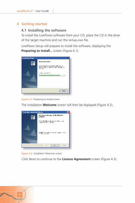
LowFlows Setup will prepare to install the software, displaying the

Preparing�to�install...�screen (Figure 4.1).

Figure�4.1 Preparing to Install screen

The installation Welcome screen will then be displayed (Figure 4.2).

Figure�4.2 Installation Welcome screen

Click Next to continue to the Licence�Agreement screen (Figure 4.3).


13

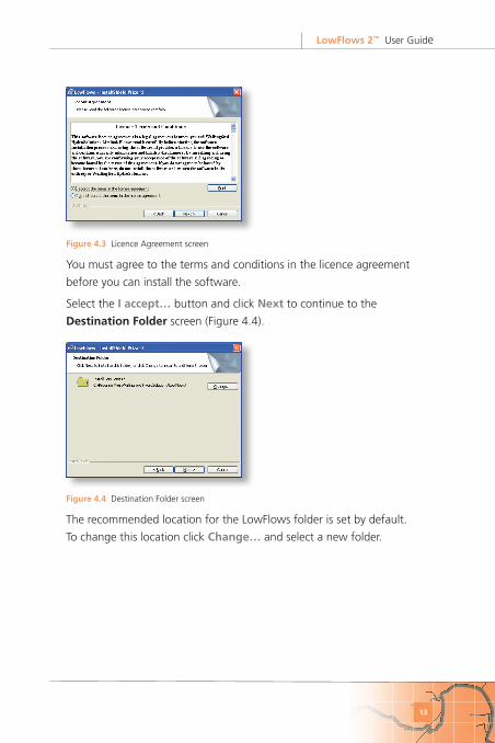
Figure�4.3 Licence Agreement screen

You must agree to the terms and conditions in the licence agreement

before you can install the software.

Select the I�accept… button and click Next to continue to the

Destination�Folder screen (Figure 4.4).

Figure�4.4 Destination Folder screen

The recommended location for the LowFlows folder is set by default.

To change this location click Change… and select a new folder.


14

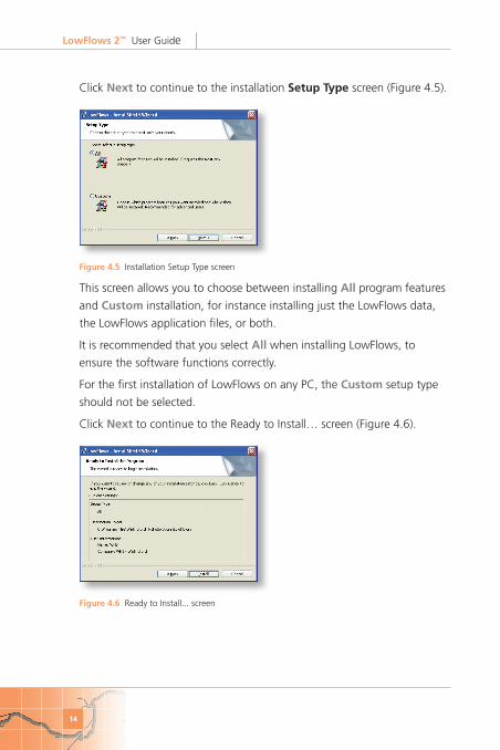
Click Next to continue to the�installation�Setup�Type�screen (Figure 4.5).

Figure�4.5 Installation Setup Type screen

This screen allows you to choose between installing All program features

and Custom installation, for instance installing just the LowFlows data,

the LowFlows application files, or both.

It is recommended that you select�All when installing LowFlows, to

ensure the software functions correctly.

For the first installation of LowFlows on any PC, the Custom�setup type

should not be selected.

Click Next to continue to the Ready to Install… screen (Figure 4.6).

Figure�4.6 Ready to Install... screen


15

Note�For future installations it may be useful to select the Custom

setup type in order to update the data only, without overwriting the

licence files. In this case select Custom and click Next to continue to the

Custom�Setup screen (Figure 4.7).

To install the data only, click on the Application icon and select [This

feature will not be available], then click Next to continue to the Ready to

Install… screen (Figure 4.6).

Figure�4.7 Custom Setup screen

Click Install to begin the installation. The Installing�LowFlows�screen

will now be displayed (Figure 4.8).

Figure�4.8 Installing LowFlows screen


16

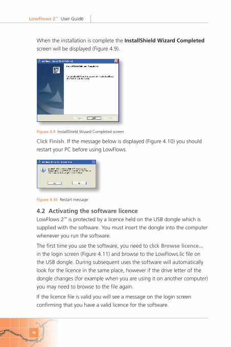
When the installation is complete the�InstallShield�Wizard�Completed

screen will be displayed (Figure 4.9).

Figure�4.9 InstallShield Wizard Completed screen

Click Finish. If the message below is displayed (Figure 4.10) you should

restart your PC before using LowFlows.

Figure�4.10 Restart message

4.2��Activating�the�software�licenceLowFlows 2™ is protected by a licence held on the USB dongle which is

supplied with the software. You must insert the dongle into the computer

whenever you run the software.

The first time you use the software, you need to click Browse�licence...�

in the login screen (Figure 4.11) and browse to the LowFlows.lic file on

the USB dongle. During subsequent uses the software will automatically

look for the licence in the same place, however if the drive letter of the

dongle changes (for example when you are using it on another computer)

you may need to browse to the file again.

If the licence file is valid you will see a message on the login screen

confirming that you have a valid licence for the software.


17

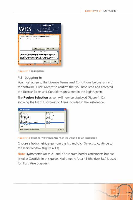
Figure�4.11 Login screen

4.3��Logging�inYou must agree to the Licence�Terms�and�Conditions before running

the software. Click Accept to confirm that you have read and accepted

the Licence Terms and Conditions presented in the login screen.

The Region�Selection screen will now be displayed (Figure 4.12)

showing the list of Hydrometric Areas included in the installation.

Figure�4.12 Selecting Hydrometric Area 45 in the England: South-West region

Choose a hydrometric area from the list and click Select to continue to

the main window (Figure 4.13).

Note Hydrometric Areas 21 and 77 are cross-border catchments but are

listed as Scottish. In this guide, Hydrometric Area 45 (the river Exe) is used

for illustrative purposes.


18

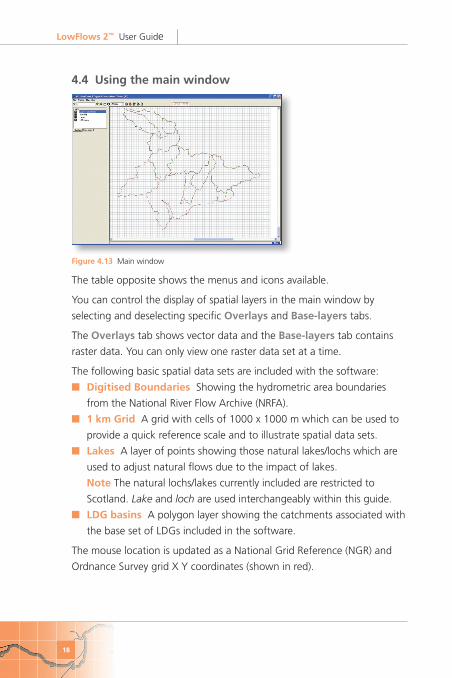
4.4��Using�the�main�window

Figure�4.13 Main window

The table opposite shows the menus and icons available.

You can control the display of spatial layers in the main window by

selecting and deselecting specific Overlays and Base-layers tabs.

The Overlays tab shows vector data and the Base-layers tab contains

raster data. You can only view one raster data set at a time.

The following basic spatial data sets are included with the software:

■ Digitised�Boundaries Showing the hydrometric area boundaries

from the National River Flow Archive (NRFA).

■ 1�km�Grid A grid with cells of 1000 x 1000 m which can be used to

provide a quick reference scale and to illustrate spatial data sets.

■ Lakes A layer of points showing those natural lakes/lochs which are

used to adjust natural flows due to the impact of lakes.

Note The natural lochs/lakes currently included are restricted to

Scotland. Lake and loch are used interchangeably within this guide.

■ LDG�basins A polygon layer showing the catchments associated with

the base set of LDGs included in the software.

The mouse location is updated as a National Grid Reference (NGR) and

Ordnance Survey grid X Y coordinates (shown in red).


19

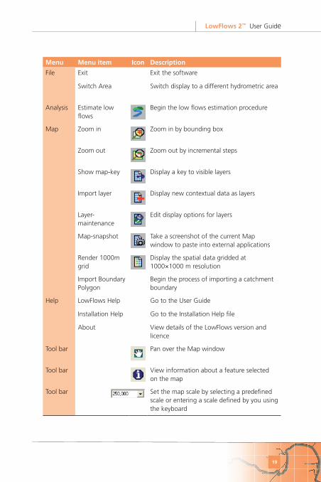
Menu Menu�item Icon Description

File Exit Exit the software

Switch Area Switch display to a different hydrometric area

Analysis Estimate low flows

Begin the low flows estimation procedure

Map Zoom in Zoom in by bounding box

Zoom out Zoom out by incremental steps

Show map-key Display a key to visible layers

Import layer Display new contextual data as layers

Layer-maintenance

Edit display options for layers

Map-snapshot Take a screenshot of the current Map window to paste into external applications

Render 1000m grid

Display the spatial data gridded at 1000×1000 m resolution

Import Boundary Polygon

Begin the process of importing a catchment boundary

Help LowFlows Help Go to the User Guide

Installation Help Go to the Installation Help file

About View details of the LowFlows version and licence

Tool bar Pan over the Map window

Tool bar View information about a feature selected on the map

Tool bar Set the map scale by selecting a predefined scale or entering a scale defined by you using the keyboard


20

5� Bringing�in�catchment�boundaries

To generate flow estimates for a catchment, you must first import an

externally defined catchment boundary.

■ Section�5.1 summarises how to define your catchment boundary

externally, for import into LowFlows. A more in-depth description of

boundary definition is given in most good hydrological textbooks.

■ Section�5.2 explains the formats you can import into LowFlows.

■ Section�5.3 takes you through importing your catchment boundary.

■ Section�5.4 explains how to delete a saved boundary.

5.1��Defining�catchment�boundariesA catchment boundary delineates the upstream area draining to the point

of interest called the catchment outlet.

Catchment boundaries should reflect the topographic and artificial

boundaries (such as catch-waters and leats) of the catchment, and may

include some allowance for groundwater divides.

You can identify catchment boundaries manually using topographic maps

of appropriate scale (typically 1:25,000 or 1:50,000). It is now common to

use digital�maps in conjunction with GIS tools, but you can use paper�

maps, in which case you need to read the string of coordinate pairs that

accurately defines the boundary from the map (see Section�5.2 for more

details).

Whichever type of map you use, the following steps are usually involved.

■ Identify the grid reference of the catchment outlet, giving particular

attention to the verification of the site in relation to upstream and

downstream confluences.

■ Identify the topographic catchment boundary using mapped

information regarding:

● river network location

● contours

● spot heights.

When you have chosen a topographic map of a scale suitable for the

catchment of interest, first select the catchment�outlet. Then start


21

defining the boundary by moving in an uphill direction, perpendicularly

crossing contours until a peak is reached.

If there is only one peak in the boundary, close the catchment boundary

by continuing downhill until the catchment outlet is reached, ensuring

that contours are crossed perpendicularly.

If the boundary passes through a number of peaks and troughs (which

is most common) the principle is the same, you continue the boundary

ensuring that contours are crossed perpendicularly. Ensure the boundary

does not cross any rivers/streams except at the catchment outlet.

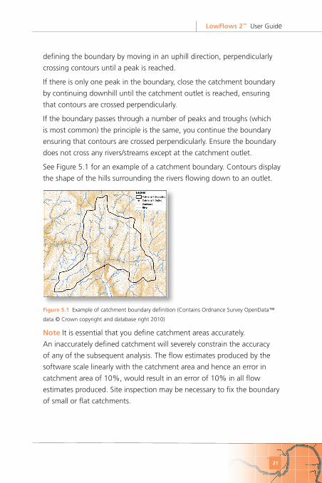
See Figure 5.1 for an example of a catchment boundary. Contours display

the shape of the hills surrounding the rivers flowing down to an outlet.

Figure�5.1 Example of catchment boundary definition (Contains Ordnance Survey OpenData™

data © Crown copyright and database right 2010)

Note It is essential that you define catchment areas accurately.

An inaccurately defined catchment will severely constrain the accuracy

of any of the subsequent analysis. The flow estimates produced by the

software scale linearly with the catchment area and hence an error in

catchment area of 10%, would result in an error of 10% in all flow

estimates produced. Site inspection may be necessary to fix the boundary

of small or flat catchments.


22

5.2��Catchment�boundary�formatsYou can import catchment boundaries into LowFlows in either of the

following formats.

■ Esri�polygon�shapefile This is a GIS file containing polygons

to represent the catchments. GIS programmes, for example Esri

ArcGIS and MapInfo, have the ability to digitise boundaries from

electronic maps. Using a GIS interface, import an appropriately scaled

topographic map and draw the catchment boundary using the ‘create

polygon’ feature in most GIS programmes. Save the boundary polygon

as a shapefile.

■ Comma-separated�values�(CSV)�file Obtain coordinate pairs of

the catchment boundary manually by either drawing the boundary

on a paper map and physically reading off the coordinates or by

reading the coordinates from an appropriate web-based map. Record

six-figure grid references for each new point of the catchment

boundary (usually indicating a change of direction), enter them

into a spreadsheet and save it as a CSV file. See Figure 5.2 for an

example spreadsheet with X (Easting) coordinates in column A,

and Y (Northing) coordinates in column B. You should list the X,Y

coordinates in order (clockwise or anticlockwise) to show the sense of

the polygon. The last point in the file should be a repeat of the first

point, to ensure polygon closure.

Figure�5.2 Catchment boundary coordinates in a spreadsheet


23

5.3��Importing�a�catchment�boundaryYou can import catchment boundaries:

■ ‘on the fly’ during the flow estimation process

via [Analysis][Estimate low flows][Use polygon from external source]

or

■ to save them for later use, as follows.

● Go to [Map][Import boundary polygon] to add a boundary polygon

from a shapefile or CSV file to the layer.

● Once you have imported the polygon or CSV file, the boundary

will be saved to the Saved�Boundaries layer (a hydrometric-area-

specific archive).

● The saved boundary can then be recalled during flow estimation via

[Analysis][Estimate low flows][Use previously imported polygon].

If you are using a shapefile, you will need to select the Import�from�

Shapefile option and browse to the Esri shapefile that contains your

boundary polygons representing catchments. Select one of the polygons

to use/import it.

If you are using a CSV file, you will need to select the Import�from�

Comma-Separated�Variables�File option and browse to the file

containing X,Y coordinates defining the extent of the required boundary

polygon. Select the file to use/import it.

Note You must inspect the boundaries saved to the Saved Boundaries

layer to ensure that you have defined the correct boundary. Incorrect

boundary definition will impact on the flow estimates you produce for the

catchment.

5.4��Deleting�a�saved�boundaryYou can delete a boundary from the Saved Boundaries layer.

Right-click the boundary in the Main window and select Delete�Saved�

Basin.


24

6� Generating�low-flow�estimates

Go to [Analysis][Estimate low flows].

If you have already imported catchment boundaries and a Saved

Boundaries layer exists, the following options will be displayed enabling

you to select the target catchment boundary you want to use.

1� Use�Polygon�from�External�Source Enables you to select a

boundary directly from a shapefile or CSV file.

2� Use�Previously-Imported�Polygon Enables you to select a boundary

from the Saved Boundaries layer (see Section�5 on importing

boundaries into LowFlows).

If no Saved Boundaries layer exists, you are restricted to the first option.

When you have selected your target boundary you need to set the

resolution of the virtual grid which defines how the catchment boundary

will be overlaid on spatial data sets. The larger the number selected the

coarser the overlay procedure. Typically, a 50m resolution is appropriate

for catchments smaller than 50km2 , a 200m resolution is appropriate

for catchments larger than 50km2 and you should consider adopting a

resolution larger than 200m for catchments larger than 1000km2.

The process of overlaying the catchment boundary on to the spatial data

sets may take a few seconds for a small catchment at low resolution, or a

few minutes for a very large catchment at high resolution.

If local�data�gauges (LDGs) are found in the vicinity of the catchment,

you need to confirm if data from these should be incorporated in the

flow estimation procedure. The incorporation of LDG data enables flow

estimates to be improved by making use of observed flows at points

upstream and/or downstream of an ungauged catchment (see Section�9).

You will also be asked if artificial�influences�should be included in

the flow estimates. If you require estimates of the natural flow regime,

select No�(see Section�6.1). If you require estimates of the flow regime

including net impacts of influences such as abstractions and discharges,

select Yes�(see Section�6.2).


25

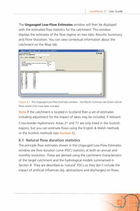
The Ungauged�Low-Flow�Estimates�window will then be displayed

with the estimated flow statistics for the catchment. This window

displays the estimates of the flow regime on two tabs:�Results�Summary

and Flow�Duration. You can view contextual information about the

catchment on the Map tab.

Figure�6.1 The Ungauged Low-Flow Estimates window – the Results Summary tab shows natural

flows where LDGs have been included

Note If the catchment is located in Scotland then a set of estimates

including adjustment for the impact of lakes may be included, if relevant.

Cross-border Hydrometric Areas 21 and 77 are only listed in the Scottish

regions, but you can estimate flows using the English & Welsh methods

or the Scottish methods (see Section�8).

6.1��Natural�flow�duration�statisticsThe principle flow estimates shown in the Ungauged Low-Flow Estimates

window are flow duration curve (FDC) statistics at both an annual and

monthly resolution. These are derived using the catchment characteristics

of the target catchment and the hydrological models summarised in

Section 8. They are described as ‘natural’ FDCs as they don’t include the

impact of artificial influences (eg. abstractions and discharges) on flows.


26

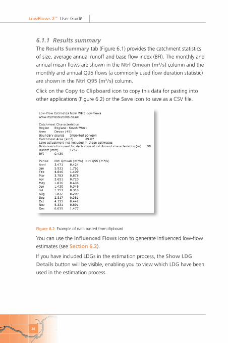
6.1.1 Results summaryThe Results�Summary tab (Figure 6.1) provides the catchment statistics

of size, average annual runoff and base flow index (BFI). The monthly and

annual mean flows are shown in the Ntrl�Qmean�(m3/s) column and the

monthly and annual Q95 flows (a commonly used flow duration statistic)

are shown in the Ntrl�Q95�(m3/s) column.

Click on the Copy�to�Clipboard icon to copy this data for pasting into

other applications (Figure 6.2) or the Save icon to save as a CSV file.

Figure�6.2 Example of data pasted from clipboard

You can use the Influenced�Flows icon to generate influenced low-flow

estimates (see Section�6.2).

If you have included LDGs in the estimation process, the Show�LDG�

Details button will be visible, enabling you to view which LDG have been

used in the estimation process.


27

6.1.2 Flow durationThe Flow�Duration tab (Figure 6.3) enables you to plot monthly and

annual FDCs by selecting tick boxes. You can select alternate axes and

switch the units between m3/s and flows expressed as a percentage of the

mean flow (annual or monthly) (%MF) using the radio buttons.

Figure�6.3 The Ungauged Low-Flow Estimates window – the Flow duration tab shows the

monthly and annual FDCs and tabulated data for the annual FDC

Click on the Copy�to�Clipboard icon or right-click in the plot area to

copy a screen shot for pasting into other applications (Figure 6.4).

Figure�6.4 Exported plot of FDCs from Flow duration tab showing May, August, Annual and

Seasonal (Oct to Mar) natural FDCs

Double right-click on any of the listed FDCs (ie double right-click on text


28

‘Annl’) to view tabulated data. Click on the Copy�to�Clipboard icon to

copy this data for pasting into other applications (spreadsheets and word

processing packages).

Clicking on the Seasonal�Series button brings up the Season�

Definition window and allows you to determine what is included in the

Results Summary and Flow duration tabs by selecting the start and end

months for FDCs covering the chosen period.

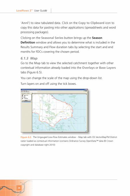
6.1.3 MapGo to the Map tab to view the selected catchment together with other

contextual information already loaded into the�Overlays or Base�Layers

tabs (Figure 6.5).

You can change the scale of the map using the drop-down list.

Turn layers on and off using the tick boxes.

Figure�6.5 The Ungauged Low-Flow Estimates window – Map tab with OS VectorMapTM District

raster loaded as contextual information (contains Ordnance Survey OpenData™ data © Crown

copyright and database right 2010)


29

6.2��Influenced-flow�estimatesThe hydrological models underpinning LowFlows enable the natural

FDC to be estimated for ungauged catchments. For catchments with

significant water-use features or artificial influences the flow regime

observed will reflect the natural FDC plus the impact of abstractions

(removing flows) and discharges (providing additional flow).

Note Impoundments/reservoirs also have an impact on the flow regime

downstream of their location, but the impact of reservoirs cannot be

modelled in the current version of LowFlows. Please contact WHS for

information on how flow estimates can be produced for catchments with

significant reservoirs.

To produce a net monthly influence profile which characterises the

net seasonal variation of water use (by type of influence) within the

catchment, you need to determine and sum the individual artificial

influences, represented by monthly profiles. In the case of a groundwater

abstraction, you need to determine the net effect of the abstraction on

surface waters, rather than the actual abstraction regime at the borehole.

This is a simplification of how groundwater abstractions are treated in

LowFlows Enterprise, where the Theis solution is applied to individual

abstraction points to determine the stream deletion factors appropriate

for the nearest river reach.

Algorithms within the software superimpose these net monthly influence

profiles onto the natural flow regime (as defined by monthly FDCs)

to produce influenced flow estimates. For instance, if significant net

abstractions occur during the summer months then the influenced flows

during these months are less than the natural flows.

If you select to include artificial influences during the low-flow estimation

process then the Set�Influence�Profile�window is displayed prior to

viewing the results in the Ungauged Low-Flow Estimates window. Enter

the net monthly influence profile for different types of influences into the

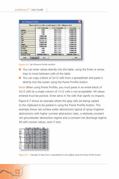
Set Influence Profile window (Figure 6.6).


30

Figure�6.6 Set Influence Profile window

■ You can enter values directly into the table, using the Enter or arrow

keys to move between cells of the table.

■ You can copy a block of 3×12 cells from a spreadsheet and paste it

directly into the screen using the Paste�Profile button.

Note When using Paste�Profile, you must paste in an entire block of

3×12 cells (ie a single column of 1×12 cells is not acceptable). All values

entered must be positive. Enter zeros in the cells that signify no impacts.

Figure 6.7 shows an example where the grey cells are being copied

to the clipboard to be pasted in using the Paste�Profile button. This

example shows net surface water abstractions typical of spray irrigation

abstractions with higher summer abstraction rates, a relatively constant

net groundwater abstraction regime and a constant net discharge regime.

All cells contain values, even if zero.

Figure�6.7 Example of data from a spreadsheet to be added using the Paste Profile button


31

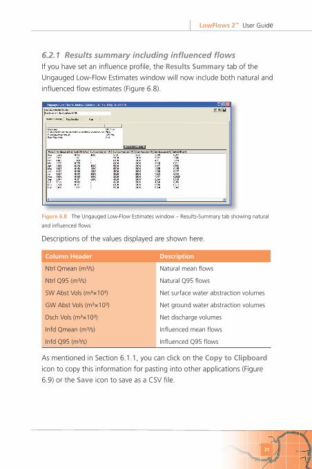
6.2.1 Results summary including influenced flowsIf you have set an influence profile, the Results�Summary tab of the

Ungauged Low-Flow Estimates window will now include both natural and

influenced flow estimates (Figure 6.8).

Figure�6.8 The Ungauged Low-Flow Estimates window – Results-Summary tab showing natural

and influenced flows

Descriptions of the values displayed are shown here.

Column�Header Description

Ntrl Qmean (m³/s) Natural mean flows

Ntrl Q95 (m³/s) Natural Q95 flows

SW Abst Vols (m³×10³) Net surface water abstraction volumes

GW Abst Vols (m³×10³) Net ground water abstraction volumes

Dsch Vols (m³×10³) Net discharge volumes

Infd Qmean (m³/s) Influenced mean flows

Infd Q95 (m³/s) Influenced Q95 flows

As mentioned in Section 6.1.1, you can click on the Copy�to�Clipboard

icon to copy this information for pasting into other applications (Figure

6.9) or the Save icon to save as a CSV file.


32

Figure�6.9 Example of data pasted from clipboard

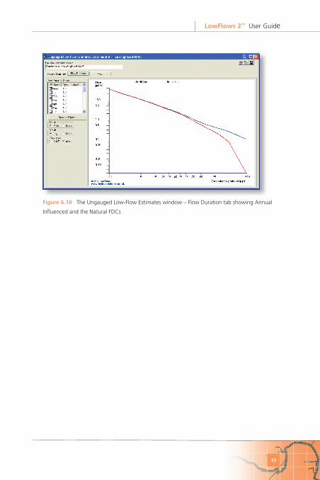
6.2.2 Flow duration including influenced flowsAs above, if you have set an influence profile, the Flow�Duration tab will

now include FDCs for the natural regime and the influenced regime. You

can display any combination of annual or monthly FDCs for the natural

or influenced regimes by using the tick boxes. Figure 6.10 shows annual

FDCs for natural and influenced regimes.

As described in Section 6.1.2, to paste from the Ungauged Low-Flow

Estimates window into other applications:

■ you can double right-click on any of the listed FDCs to display

tabulated data and copy it to the clipboard

■ you can right-click within the plot area or click on the Copy�to�

Clipboard icon and copy a screen shot to the clipboard.


33

Figure�6.10 The Ungauged Low-Flow Estimates window – Flow Duration tab showing Annual

Influenced and the Natural FDCs


34

7� Using�contextual�data

You can import Spatial data sets to provide contextual information. For

example, Ordinance Survey tiles can be added as a base layer to the map

windows.

Go to [Map][Import layer] to define the type of data you are going to

import and how it should be imported. You will be able to select the

imported layers in the Main window on either the Overlays or Base�

Layers tabs.

Go to [Map][Layer-maintenance] to edit your imported layers. You can

set attributes such as line colour, thickness, point symbols and polygon

transparency.

7.1��Importing�contextual�dataYou can import contextual data in the form of vector data (SHP) or

raster data (BMP and TIF) and view it through the geographical interface

of LowFlows.

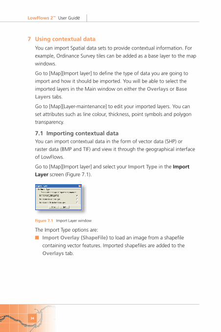
Go to [Map][Import layer] and select your Import�Type in the Import�

Layer�screen (Figure 7.1).

Figure�7.1 Import Layer window

The Import Type options are:

■ Import�Overlay�(ShapeFile) to load an image from a shapefile

containing vector features. Imported shapefiles are added to the

Overlays tab.


35

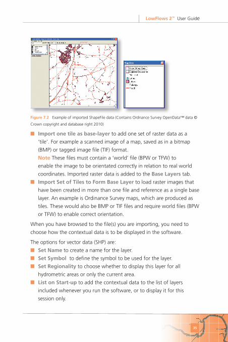
Figure�7.2 Example of imported ShapeFile data (Contains Ordnance Survey OpenData™ data ©

Crown copyright and database right 2010)

■ Import�one�tile�as�base-layer to add one set of raster data as a

‘tile’. For example a scanned image of a map, saved as in a bitmap

(BMP) or tagged image file (TIF) format.

Note These files must contain a ‘world’ file (BPW or TFW) to

enable the image to be orientated correctly in relation to real world

coordinates. Imported raster data is added to the Base�Layers tab.

■ Import�Set�of�Tiles�to�Form�Base�Layer to load raster images that

have been created in more than one file and reference as a single base

layer. An example is Ordinance Survey maps, which are produced as

tiles. These would also be BMP or TIF files and require world files (BPW

or TFW) to enable correct orientation.

When you have browsed to the file(s) you are importing, you need to

choose how the contextual data is to be displayed in the software.

The options for vector data (SHP) are:

■ Set�Name to create a name for the layer.

■ Set�Symbol� to define the symbol to be used for the layer.

■ Set�Regionality to choose whether to display this layer for all

hydrometric areas or only the current area.

■ List�on�Start-up�to add the contextual data to the list of layers

included whenever you run the software, or to display it for this

session only.


36

The options for raster data (BMP and TIF) are:

■ Set�Name as for vector data.

■ List�on�Start-up�as for vector data.

■ Set�Regionality as for vector data.

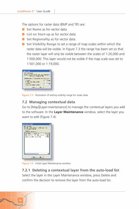
■ Set�Visibility�Range to set a range of map scales within which the

raster data will be visible. In Figure 7.3 the range has been set so that

the raster layer will only be visible between the scales of 1:20,000 and

1:500,000. This layer would not be visible if the map scale was set to

1:501,000 or 1:19,000.

Figure�7.3 Illustration of setting visibility range for raster data

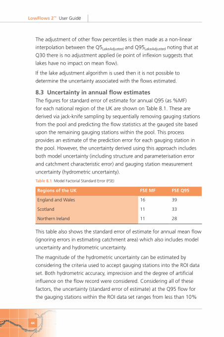
7.2��Managing�contextual�dataGo to [Map][Layer-maintenance] to manage the contextual layers you add

to the software. In the Layer�Maintenance window, select the layer you

want to edit (Figure 7.4).

Figure�7.4 Initial Layer-Maintenance window

7.2.1��Deleting�a�contextual�layer�from�the�auto-load�listSelect the layer in the Layer Maintenance window, press Delete and

confirm the decision to remove the layer from the auto-load list.


37

Note The source vector/raster data is not deleted during this process, it

is just removed from the list of layers that are automatically loaded into

LowFlows.

Note The Saved Boundaries layer is a special data layer that represents

the archive of imported catchment boundaries (see Section�5). If this

layer is deleted from the auto-load list, you will not be able to use

catchment polygons from this layer to perform low-flow estimates via the

Use�Previously-Imported�Polygon option (see Section�6).

7.2.2 Editing the properties of a contextual layerSelect the layer and then right-click on it in the Layer Maintenance

window to access the editing options. The different options are available

for vector and raster data sets.

The edit options for vector data (from Overlays) are:

General edits (Figure 7.5)

■ Name as in Set Name when importing the data.

Note Do not change the name of the Saved Boundaries layer, as it is

referenced by the software. Other editing options are available for this

layer.

■ Regionality as in Set Regionality when importing the data.

■ Initial�Visibility to define whether the layer will appear automatically

when you run the software or whether you must select it manually

from the Overlays tab.

■ Set�Symbol as in Set Symbol when importing the data.

Figure�7.5 Editing vector data (Stage I) – general edits


38

Setting symbols (Figure 7.6)

The options available at the Set�Symbol window depend on the type of

data in the ShapeFile, eg point, line or polygon. The example shown here

is for the Saved�Boundaries layer of polygons. Editing options are self-

explanatory and the preview box shows the impact of choices made.

Figure�7.6 Editing vector data (Stage II) – setting symbols.

The edit options for raster data (from base layers) are: (Figure 7.7).

■ Name as in Set Name when importing the data.

■ Regionality as in Set Regionality when importing the data.

■ Visibility�Range as in Set Visibility Range when importing the data.

■ Initial�Visibility defines whether the layer automatically appears

when the software to define whether the layer will appear

automatically when you run the software or whether you must select

it manually from the Base Layers tab.

Figure�7.7 Editing raster data.

When you made your chosen edits click Done.


39

8� The�hydrological�models�in�LowFlows

The hydrological estimation models used in the software are derived from

the LowFlows 2000 software system that was developed jointly by the

Centre for Ecology and Hydrology (CEH) and the Environment Agency of

England and Wales (EA), the Scottish Environmental Protection Agency

(SEPA) and the Northern Ireland Environment Agency (NIEA). The model

structures are described in detail by Young et al. (2003) and Holmes et al.

(2002a, 2002b).

In summary, these models enable annual and monthly flow duration

curve (FDC) statistics to be estimated at the ungauged site.

■ An annual mean flow model – used as an annual runoff grid (1km

resolution) developed by a variety of methods.

■ Region of influence (ROI) models for annual and monthly flow

duration statistics standardised by mean flow. The standardised

statistics are then rescaled by the respective estimates of mean flow.

■ An ROI model for estimating monthly mean flows, when expressed as

fractions of annual runoff.

The software also provides an estimate of the base flow index (BFI)

(Gustard et al. 1992), based upon the Hydrology of soil types (HOST)

classification (Boorman et al. 1995).

The hydrological models are summarised below.

Note Section 9 describes how local data gauges (LDGs) are used to

improve the initial natural flow estimates produced by the hydrological

models.

8.1��Estimation�of�annual�mean�flowThe estimation of annual mean flow is based on a 1km2 grid of long-term

average annual runoff underpinning the software.

■ In England, Wales and Scotland the runoff grid was developed using

outputs from a deterministic water balance model using observed

data from over 500 gauged catchments. The development of this grid

is described in detail by Holmes et al. (2002a).


40

■ In Northern Ireland the runoff grid was developed using an annual

water balance model to predict runoff from rainfall and potential

evaporation with a reduction factor of 0.86 applied to potential

evaporation.

The mean flow can be estimated from the average annual runoff depth

(RO) in mm over the whole catchment (AREA in km2) using the equation:

MF = RO × AREA × CONST

The long-term mean flow is used to scale the annual FDC so that the

range of flows can be expressed in cubic metres per second (m3/s).

8.2��Estimation�of�the�annual�flow�duration�curve�An assumption central to the estimation procedures is that when

low flows are expressed as a percentage of the long-term mean flow

(standardised), the dependencies on the climatic variability across the

country and the effect of catchment area are minimised. As a result, the

estimation of standardised FDCs is largely dependent on the hydro-

geological and soils characteristics of the catchment. The software uses

the HOST classification of soils (Boorman et al, 1995) to represent these

characteristics. Research has shown that climate also exerts an influence

on stream flow recessions, the strong east–west rainfall gradient across

Scotland, for example. Hence, catchment mean annual runoff (RUNOFF) is

used to explain observed variation in flow variability.

The models used to estimate the FDC statistics are based on a ROI

regionalisation approach. The ROI method develops an estimate of a flow

statistic or hydrologic parameter at an ungauged target catchment from

observed values of that flow statistic or hydrologic parameter made at a

number of gauged catchments which are considered to be similar to the

ungauged catchment. Similarity is measured by catchment characteristics

that can be obtained for any ungauged catchment in the UK. Implicit

in the methodology is a data set of good quality natural observed flow

records for a wide range of catchment types.


41

The ROI based model seeks to reduce the variability of the dependent

variable within the data set, by reducing it to a much smaller region of

catchments that are similar to the target catchment. In application to a

catchment, the methods can be summarised as the following steps:

1� The similarity of the target catchment to donor catchments in the ROI

data set is calculated as a weighted Euclidean distance:

where deit is the weighted Euclidean distance from the target

catchment, t, to donor catchment, i, in the ROI data set, Wm is the

weight applied to catchment characteristic, m, and Xmi is the

standardised value of catchment characteristic, m, for catchment, i.

� The catchment characteristics used, Xm, are the fractional extents

of the HOST classes within a catchment and the logarithm (10) of

mean annual runoff (LOGRUNOFF) value for a catchment. The use

of weights for individual HOST classes reflects the fact that relatively

small proportions of certain HOST classes, especially HOST classes of

permeable soil overlying permeable geologies, strongly influence the

variability of the flows within a catchment. The weight assigned to the

LOGRUNOFF value reflects the relative importance of climatological

factors.

2� A region is formed around the target catchment by ranking all of the

catchments in the data pool by their weighted Euclidean distance and

selecting the n catchments that are closest to the target catchment.

3� A standardised annual FDC is estimated for the target catchment by

taking an inverse weighted combination of the standardised FDCs for

the gauged catchments in the region. Thus, greater weight was given

to catchments that are more similar in HOST characteristics to the

target catchment.


42

This is expressed mathematically as:

� where QP(×)ESTt is the estimate of the flow for the target catchment,

t, at exceedence percentile P(×), QP(×)OBSi is the observed value

of QP(×) for the ith source catchment in the region of n catchments

closest to the target catchment and dei is the weighted Euclidean

distance of the ith catchment from the target catchment, t.

� This procedure is used for estimation in England, Wales, Scotland and

Northern Ireland.

8.2.1 Adjustment of FDCs in Scotland for the influence of natural lochsThe original LowFlows research in Scotland developed a procedure for

estimating the influence of the many natural lochs in Scotland on the

estimation of flow duration statistics. The storage associated with natural

lochs within a catchment tends to maintain (increase) base flow and

hence low flows, and attenuate high flows (all other factors being equal).

It is important to note the distinction between a natural loch and a

reservoir or managed loch. The influence of the latter on the downstream

flow regime may be complex and will be directly related to how outflows

from the reservoir are managed by the operator.

The original Loch Adjustment Procedure was revised in collaboration with

SEPA. The new procedure is based on available data from a relatively small

number of larger Scottish lochs, supplemented by data from Cumbrian

lakes and is currently only deployed within LowFlows in Scotland for

significant lochs identified in consultation with SEPA. Recommendations

have been presented to SEPA to collect additional data to both validate

the algorithm and provide data sets for smaller lochs. The model is not


43

used in the current LowFlows software for England, Wales and Northern

Ireland, although this position will be reviewed in the future.

When used in the LowFlows software, a Loch Adjustment Factor (LAF) is

calculated for each loch in the target (ungauged) catchment based on the

ratio of the surface area of the loch/lake (LA) and the catchment area of

the loch/lake (LCA) as follows.

LAF = 0 if LA <0.1km2

LAF = 0 if LCA <1.5km2

LAF = 0 for case LA/LCA < 2%

for case 2% ≤ LA/LCA < 10%

for case LA/LCA ≥ 10%

Where LA = Loch/Lake surface area (km2)

LCA = Catchment area above lake (km2)

LAF = Loch/Lake Adjustment Factor (%MF)

An adjustment to the raw estimate of Q95 as %MF obtained from the

ROI algorithm (Q95Raw) for the target catchment is then calculated as:

in %MF

where ADJQ95 is the adjustment to Q95 in %MF for the target catchment,

LAFi is the LAF value for the ith loch, Q95i is the natural Q95 estimate at

the outlet of the ith loch (if the loch was not present in the catchment),

LCA is the catchment area of the ith loch and CA is the catchment area of

the target catchment.

Hence the adjusted value of the Q95(%MF) for the target catchment is

Q95LakeAdjusted = Q95Raw + ADJQ95 in %MF

The adjustment statistic for high flows is defined at Q5 to be:


44

The adjustment of other flow percentiles is then made as a non-linear

interpolation between the Q5LakeAdjusted and Q95LakeAdjusted noting that at

Q30 there is no adjustment applied (ie point of inflexion suggests that

lakes have no impact on mean flow).

If the lake adjustment algorithm is used then it is not possible to

determine the uncertainty associated with the flows estimated.

8.3��Uncertainty�in�annual�flow�estimatesThe figures for standard error of estimate for annual Q95 (as %MF)

for each national region of the UK are shown on Table 8.1. These are

derived via jack-knife sampling by sequentially removing gauging stations

from the pool and predicting the flow statistics at the gauged site based

upon the remaining gauging stations within the pool. This process

provides an estimate of the prediction error for each gauging station in

the pool. However, the uncertainty derived using this approach includes

both model uncertainty (including structure and parameterisation error

and catchment characteristic error) and gauging station measurement

uncertainty (hydrometric uncertainty).

Table�8.1 Model Factorial Standard Error (FSE)

Regions�of�the�UK FSE�MF FSE�Q95

England and Wales 16 39

Scotland 11 33

Northern Ireland 11 28

This table also shows the standard error of estimate for annual mean flow

(ignoring errors in estimating catchment area) which also includes model

uncertainty and hydrometric uncertainty.

The magnitude of the hydrometric uncertainty can be estimated by

considering the criteria used to accept gauging stations into the ROI data

set. Both hydrometric accuracy, imprecision and the degree of artificial

influence on the flow record were considered. Considering all of these

factors, the uncertainty (standard error of estimate) at the Q95 flow for

the gauging stations within the ROI data set ranges from less than 10%


45

for the highest quality stations to 30% for the lowest quality stations.

Note The lowest quality stations are still regarded by measuring

authorities as representing an acceptable measurement of low flows.

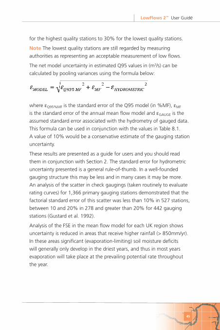
The net model uncertainty in estimated Q95 values in (m3/s) can be

calculated by pooling variances using the formula below:

where εQ95%MF is the standard error of the Q95 model (in %MF), εMF

is the standard error of the annual mean flow model and εGAUGE is the

assumed standard error associated with the hydrometry of gauged data.

This formula can be used in conjunction with the values in Table 8.1.

A value of 10% would be a conservative estimate of the gauging station

uncertainty.

These results are presented as a guide for users and you should read

them in conjunction with Section 2. The standard error for hydrometric

uncertainty presented is a general rule-of-thumb. In a well-founded

gauging structure this may be less and in many cases it may be more.

An analysis of the scatter in check gaugings (taken routinely to evaluate

rating curves) for 1,366 primary gauging stations demonstrated that the

factorial standard error of this scatter was less than 10% in 527 stations,

between 10 and 20% in 278 and greater than 20% for 442 gauging

stations (Gustard et al. 1992).

Analysis of the FSE in the mean flow model for each UK region shows

uncertainty is reduced in areas that receive higher rainfall (> 850mm/yr).

In these areas significant (evaporation-limiting) soil moisture deficits

will generally only develop in the driest years, and thus in most years

evaporation will take place at the prevailing potential rate throughout

the year.


46

8.4��Estimation�of�monthly�flow�duration�statisticsThe development of methods for estimating monthly statistics within

the LowFlows software systems was driven by the desire to estimate

influenced flow regimes in which artificial influences are incorporated

as a monthly influence profile (Young et al. 2003). This allows both the

seasonal variations in flows and influences to be taken into account.

The method used to estimate standardised monthly FDCs is identical to

the ROI approach for the annual FDC outlined in Section 8.1.

8.5��Estimation�of�monthly�mean�flowAn estimate of monthly mean flow is required to rescale the standardised

monthly FDCs derived as described previously.

In UK catchments, the distribution of the total volume of annual runoff

between the months of the year is clearly a function of the magnitude

and seasonal distribution of rainfall, the strong seasonality of evaporation

demand and the presence of soil moisture deficits that suppress the

generation of runoff. The distribution is also strongly influenced by

catchment hydrogeology. For example, the lowest flows in groundwater-

fed catchments will typically occur in the autumn when groundwater

levels are at their lowest, whilst the lowest flows in low-storage

impermeable catchments will typically occur in the summer months when

evaporation demand is highest. The distribution of annual runoff within

dry impermeable catchments will tend to be more skewed towards the

winter months than in wet impermeable catchments. This is a function of

the enhanced role that soil moisture deficits play in suppressing summer

runoff in dryer catchments.

An ROI model was developed to estimate the percentage of the annual

runoff volume that occurs within each month, termed the monthly runoff

volume (MRV), using catchment characteristics of hydrogeology (HOST)

and RUNOFF (the balancing of rainfall and evaporative demand).

The MRV ROI model differs to the one used to determine flow duration

statistics and the steps are detailed opposite.


47

1� The similarity of the target catchment to donor catchments in the ROI

data set is calculated as a weighted Euclidean distance, identical to

that used in the flow duration statistic algorithm (Section 8.1):

� where deit is the weighted Euclidean distance from the target

catchment, t, to donor catchment, i, in the ROI data set, Wm is

the weight applied to catchment characteristic, m, and Xmi is the

standardised value of catchment characteristic, m, for catchment, i.

2� A region is formed around the target catchment by ranking all of the

catchments in the data pool by their weighted Euclidean distance and

selecting the n catchments that are closest to the target catchment.

3� The modulus of the difference between the target and donor

catchment LOGRUNOFF values (DIFFRO) is calculated for all n donors in

the region.

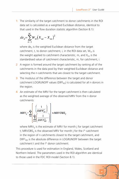
4� An estimate of the MRV for the target catchment is then calculated

as the weighted average of the observed MRV from the n donor

catchments:

� where MRVtj is the estimate of MRV for month j for target catchment

t; MRVOBSij is the observed MRV for month j for the ith catchment

in the region of n catchments closest to the target catchment, and

DIFFiRO is the absolute difference in LOGRUNOFF between the target

catchment t and the ith donor catchment.

This procedure is used for estimation in England, Wales, Scotland and

Northern Ireland. The parameters used in the ROI algorithm are identical

to those used in the FDC ROI model (Section 8.1).


48

8.6��Estimation�of�base�flow�indexThe base flow index (BFI) can be conceptualised as the proportion of the

long-term river flow considered to be derived from groundwater stores,

hence varies between 0 and 1. When considering an observed flow

record, the BFI is calculated as the ratio of the area under the base flow

hydrograph to the area under the flow hydrograph. In the UK, permeable

catchments (eg chalk) have higher values of BFI than impermeable

catchments (eg clay).

During the development of the HOST classification Boorman et al. (1995)

derived bounded linear regression equations relating the fractional

extents of HOST classes to catchment BFI. A similar model structure has

been used in the LowFlows software using coefficients refined by recent

data sets. Three sets of coefficients are used, one for England & Wales,

one for Scotland and one for Northern Ireland.


49

9� Incorporating�local�data

The regional hydrologic models in LowFlows do not explicitly take into

account local hydrometric data in the context of the estimation of long-

term mean flow and only partially within the estimation of the flow

duration curve (FDC). The estimation of FDCs in catchments with locally

gauged data can be improved by explicitly incorporating this data.

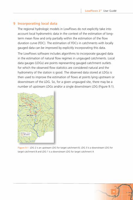
The LowFlows software includes algorithms to incorporate gauged data

in the estimation of natural flow regimes in ungauged catchments. Local

data gauges (LDGs) are points representing gauged catchment outlets

for which the observed flow statistics are considered natural and the

hydrometry of the station is good. The observed data stored at LDGs is

then used to improve the estimation of flows at points lying upstream or

downstream of the LDG. So, for a given ungauged site, there may be a

number of upstream LDGs and/or a single downstream LDG (Figure 9.1).

Figure�9.1 LDG 2 is an upstream LDG for target catchment B, LDG 3 is a downstream LDG for

target catchment B and LDG 1 is a downstream LDG for target catchment A


50

9.1��Upstream�LDGsIn the case of one or more upstream LDGs, the flow at the ungauged

catchment may be considered to be the total of all the flows recorded

at the upstream LDGs, with additional runoff from the incremental area,

which is the area in the ungauged catchment which is not included in any

of the LDG sub-catchments.

The mean flow for the incremental area is determined by subtracting the

total LowFlows runoff-derived mean flow for all of the LDG catchments,

from the LowFlows runoff-derived mean flow for the ungauged

catchment.

The estimated mean flow for the ungauged catchment is obtained from

the sum of the runoff-derived mean flow for the incremental area and

the sum of the recorded mean flows at all of the upstream LDGs.

Where the total area of the LDG catchments is small in comparison to

the area of the ungauged catchment, estimates of mean flow using this

method are unlikely to be strongly influenced by the upstream LDG data

and will be similar to the mean flow estimated by the runoff method

within LowFlows.

The Q95 value for the incremental area is estimated using the LowFlows

ROI algorithm. The Q95 statistic for the ungauged catchment is estimated

as the sum of the measured Q95 values for all LDG catchments, and the

ROI-estimated Q95 value for the incremental area. Other flow percentiles

are estimated using a similar methodology.

9.2��Downstream�LDGsWhere a downstream LDG exists then the flow at the ungauged

catchment may be considered to be the difference between the flow

recorded at the downstream LDG and the flows from the incremental

area catchment between the ungauged site and the LDG.

The mean flow for the incremental area in this case is determined

by subtracting the total runoff-derived mean flow for the ungauged

catchment from the runoff-derived mean flow for the LDG catchment.


51

For downstream local data, a first estimate of the mean flow for the

ungauged catchment is obtained by subtracting the runoff-derived mean

flow in respect of the incremental area from the mean flow at the LDG.

Since flows from the ungauged catchment may represent only a small

proportion of flows recorded at a downstream gauge, a weighting

factor (derived from the ratio of the estimated mean flows for the

ungauged and LDG sites) is applied to the first estimate of mean

flow for the ungauged catchment, to derive a weighted estimate of a

runoff correction term. The runoff for the ungauged catchment is then

estimated as the sum of the un-adjusted runoff estimate and the runoff

correction term.

An analogous procedure is also used for estimating an adjusted-at-site

estimate of the Q95 flow (retaining the MF derived weighting factor).

Other flow percentiles are adjusted following the same methodology.

Note If the ungauged catchment represents less than 10% of the

downstream LDG catchment area then the downstream LDG is not used

to adjust the estimates at the ungauged site.

If including a downstream LDG results in negative flows being predicted

for the ungauged site, it is excluded from the adjustment process.

9.3��Using�both�upstream�and�downstream�LDGsWhere both upstream LDGs and a downstream LDG exist then both

types of gauged data are used to improve the estimation of flows at the

ungauged site. Upstream LDGs are used to derive a first correction for

catchment MF and Q95, which is then improved further by adjustment

considering the downstream LDG.

9.4��LDGs�preloaded�in�the�softwareThe LowFlows software is preloaded with a base set of LDGs that were

derived for the Environment Agency of England and Wales, the Scottish

Environment Protection Agency and the Northern Ireland Environment

Agency. These are the ROI gauges used in the estimation methodology.


52

10�References

Boorman�D�B,�Hollis�J�M�and�Lilly�A (1995)

Hydrology of soil types: a hydrologically-based classification of the soils of

the United Kingdom. Report 126, Institute of Hydrology, Wallingford.

Gustard�A,�Bullock�A,�and�Dixon�JM (1992)

Low-flow estimation in the United Kingdom. Report 108, Institute of

Hydrology, Wallingford.

Holmes�MGR,�Young�AR,�Gustard�AG�and�Grew�R (2002a)

A Region of Influence approach to predicting flow duration curves

within ungauged catchments. Hydrology and Earth System Sciences 6(4)

721–731.

Holmes�MGR,�Young�AR,�Gustard,�AG�and�Grew�R (2002b)

A new approach to estimating mean flow in the United Kingdom.

Hydrology and Earth System Sciences. 6(4) 709–720.

Holmes�MGR�and�Young�AR (2002)

Estimating seasonal low-flow statistics in ungauged catchments. In Proc.

British Hydrological Society 8th National Symposium, Birmingham, 2002,

97 102.

Institute�of�Hydrology (1992)

Low-flows estimation within the United Kingdom. Report 108. Institute of

Hydrology, Wallingford.

Young�AR,�Grew�R�and�Holmes�MGR (2003)

Low Flows 2000: A national water resources assessment and decision

support. Water Science and Technology, 48 (10).


53

11�Glossary

Artificial�influences Abstractions, discharges and impoundments

(reservoirs). These features can impact on rivers by reducing flows

(abstractions and storage of water in impoundments during winter) or

increasing flows (discharges and releases from impoundments in summer)

to produce an ‘artificially influenced’ flow regime. This influenced regime

differs to the ‘natural’ flow regime which represents flows that would

naturally occur in the catchment (assuming no anthropogenic influences).

Note The impact of reservoirs cannot be modelled in the current version

of LowFlows. Please contact WHS for information on how flow estimates

can be produced for catchments with significant reservoirs.

Base�flow�index (BFI) The proportion of the long-term river flow

considered to be derived from groundwater stores, hence varies between

0 and 1. When considering an observed flow record, the BFI is calculated

as the ratio of the area under the base flow hydrograph to the area under

the flow hydrograph. In the UK, permeable catchments (eg chalk) have

higher values of BFI than impermeable catchments (eg clay) (Figure 11.1).

Figure�11.1 Base flow hydrographs from chalk (left) and clay (right) catchments showing that the

BFI for chalk is higher than the BFI for clay

The model used to estimate BFI in the software is that described

in Boorman et al. (1995) and is based on the relationship between

hydrogeology/soils and catchment response to rainfall.

Catchment�boundary The upstream area draining to the point of

interest called the catchment�outlet. This area can be conceptualised

by considering the downhill direction in which a drop of water would


54

move. If the direction is towards the point of interest, it lies within the

catchment boundary and if it moves away it does not. So, based upon

topography, the catchment boundary separates the area which drains to

the point of interest and the areas that drain away.

Flow�duration�curve (FDC) A graphic representation of the percentage

of time a particular river flow is equalled or exceeded. A popular design

statistic is the Q95 flow; this is the flow that is equalled or exceeded for

95% of the time. The FDC is therefore an inverse cumulative frequency

diagram of flow values.

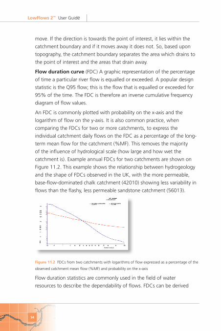
An FDC is commonly plotted with probability on the x-axis and the

logarithm of flow on the y-axis. It is also common practice, when

comparing the FDCs for two or more catchments, to express the

individual catchment daily flows on the FDC as a percentage of the long-

term mean flow for the catchment (%MF). This removes the majority

of the influence of hydrological scale (how large and how wet the

catchment is). Example annual FDCs for two catchments are shown on

Figure 11.2. This example shows the relationship between hydrogeology

and the shape of FDCs observed in the UK, with the more permeable,

base-flow-dominated chalk catchment (42010) showing less variability in

flows than the flashy, less permeable sandstone catchment (56013).

Figure�11.2 FDCs from two catchments with logarithms of flow expressed as a percentage of the

observed catchment mean flow (%MF) and probability on the x-axis

Flow duration statistics are commonly used in the field of water

resources to describe the dependability of flows. FDCs can be derived


55

from observed data for gauged catchments, but estimates of resource

availability are often required in catchments without gauging stations.

The models used in the LowFlows software estimate a standardised

annual FDC (as %MF) for the ungauged catchment based on catchment

characteristics are described by Holmes et al. (2002a). An estimate of

mean flow for the catchment is derived by models described by Holmes

et al. (2002b) and used to re-scale the FDC to flow units. The estimation

of seasonal FDCs is described by Holmes and Young (2002).

Hydrometric�areas Divisions of the United Kingdom which represent the

main river basins (Figure 11.3). See information produced by the NRFA.

Figure�11.3 UK Hydrometric Areas and National Grid coordinates


56

Influenced�flow�estimates Estimates of flow produced by LowFlows

which include the impact of any artificial influences you have entered via

the net monthly influence profile. These estimates represent the long-

term flow conditions that would be observed in a river where a number

of artificial influences were operating in a catchment.

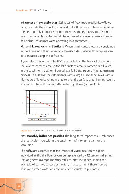
Natural�lakes/lochs�in�Scotland When significant, these are considered

in LowFlows and their impact on the estimated natural flow regime can

be simulated using the software.

If you select this option, the FDC is adjusted on the basis of the ratio of

the lake catchment area to the lake surface area, summed for all lakes

in the catchment. Section 8 contains a full description of the adjustment

process. In essence, for catchments with a large number of lakes with a

high ratio of lake catchment area to the lake surface area the net result is

to maintain base flows and attenuate high flows (Figure 11.4).

Figure�11.4 Example of the impact of lakes on the natural FDC

Net�monthly�influence�profiles The long-term impact of all influences

of a particular type within the catchment of interest, at a monthly

resolution.

The software assumes that the impact of water use/return for an

individual artificial influence can be represented by 12 values, reflecting

the long-term average monthly rates for that influence. Taking the

example of surface water abstraction, in a catchment there may be

multiple surface water abstractions, for a variety of purposes.


57

You need to sum these impacts to derive a net monthly influence profile

for all surface water abstractions applicable for that catchment.

Figure 11.5 illustrates a simple example where a catchment has one spray

irrigation abstraction and one abstraction for industrial processes and a

net profile is constructed by summing the two.

Figure�11.5 Example of summation of monthly abstraction profiles

The three types of profiles that can be entered are:

■ Surface�water�abstractions�(SW_ABS) Abstractions directly from

streams and rivers. The monthly profile represents the average

monthly volumes abstracted from the river, as the impact is a

direct impact, summed for all surface water abstractions within the

catchment.

■ Groundwater�abstractions�(GW_ABS)�Abstractions made from

boreholes and wells which have an indirect impact on the rivers as

a result of the complex response of stream flow to the pumping of

water from an unconfined, or semi-confined aquifer. For an individual

borehole, the impact of the abstraction on the river flow is dependent

upon factors including:

● the bulk aquifer hydrogeology and geometry

● the distance of the borehole to the connected stream

● the seasonality of pumping

● the pumping rate

● the degree of hydraulic connection between stream and aquifer

● features such as swallow holes and spring lines.


58

You need to assess the impact of each groundwater abstraction, and

determine the long-term average monthly profile representing the

impact on the nearest/connected surface water, considering the above

factors. You then sum these profiles to give a net monthly influence

profile for groundwater abstractions in the catchment, which you can

enter into the software.

Note This is a simplification of how groundwater abstractions are

treated in LowFlows Enterprise, where the Theis solution is applied to

individual abstraction points to determine the stream deletion factors

appropriate for the nearest river reach.

■ Discharges (DIS)�Discharges made directly to rivers. Discharges to

boreholes/groundwater sinks are not currently modelled. The monthly

profile represents the average monthly impact of all discharges to

surface waters in the catchment.

NRFA The National River Flow Archive. Part of the Centre for Hydrology

and Ecology, Wallingford, OXON OX10 8BB. The Archive is responsible for

the acquisition, archiving and validation of hydrological data for the entire

United Kingdom and publishes the Hydrometric Register and Statistics.

http://www.ceh.ac.uk/data/nrfa/


59

lowflows 2 smaller groundwater catchments river flows may be ... installing all program features and...

Documents