ls-dyna analysis for structural · pdf filels-dyna® analysis for structural mechanics an...
TRANSCRIPT

LS-DYNA® Analysis for Structural Mechanics
An overview of the core analysis features used by LS-DYNA® to simulate highly nonlinear static and dynamic behavior in engineered structures and systems.

LS-DYNA Analysis for Structural Mechanics 2017
Proprietary Information to Predictive Engineering, Please Do Not Copy or Distribute without Written Permission Page 2 of 167
Acknowledgements
These notes were constructed from numerous sources but special thanks should be given to the following people:
Technical Support Team at Livermore Software and Technology Corporation (LSTC)
With special mention to:
Satish Pathy, LSTC
Jim Day, LSTC
Philip Ho, LSTC
And the invaluable team at:
DYNAmore, Gmbh, Germany
Trademarks:
LS-DYNA® and LS-PrePost® are registered and protected trademarks of LSTC.
Disclaimer:
The material presented in this text is intended for illustrative and educational purposes only. It is not intended to be exhaustive or to apply to any particular engineering design or problem. Predictive Engineering nor the organizations mentioned above and their employees assumes no liability or responsibility whatsoever to any person or company for any direct or indirect damages resulting from the use of any information contained herein.
LS-DYNA Analysis for Structural Mechanics 2017
Proprietary Information to Predictive Engineering, Please Do Not Copy or Distribute without Written Permission Page 3 of 167
COURSE OUTLINE 1. INTRODUCTION ...............................................................................................................................................................................................10
1.1 WHAT THE STUDENT CAN EXPECT ......................................................................................................................................................................10
1.2 WHAT WE COVER ............................................................................................................................................................................................10
1.3 HOW WE DO IT ...............................................................................................................................................................................................10
1.4 GENERAL APPLICATIONS ...................................................................................................................................................................................11
1.5 SPECIFIC APPLICATIONS (COURTESY OF PREDICTIVE ENGINEERING) ............................................................................................................................12
2. IMPLICIT VERSUS EXPLICIT ANALYSIS .............................................................................................................................................................18
2.1 WHAT WE ARE SOLVING ..................................................................................................................................................................................18
2.2 EXPLICIT (DYNAMIC) – ONE MUST HAVE “MASS” TO MAKE IT GO .............................................................................................................................19
2.3 IMPLICIT (DYNAMIC).........................................................................................................................................................................................19
3. FUNDAMENTAL MECHANICS OF EXPLICIT ANALYSIS .....................................................................................................................................20
3.1 TIME STEP SIGNIFICANCE ..................................................................................................................................................................................20
Explicit Time Integration ...................................................................................................................................................................21 3.1.1
3.2 TIME STEP SIGNIFICANCE (COURANT-FRIEDRICHS-LEWY (CFL) CHARACTERISTIC LENGTH) .............................................................................................22
3.3 MASS SCALING: (EVERYBODY DOES IT BUT NOBODY REALLY LIKES IT) .......................................................................................................................23
Workshop: 1 - LS-DYNA Mass Scaling Basics ....................................................................................................................................24 3.3.1
Instructor Led Workshop: 2 - Mass Scaling Advanced .....................................................................................................................26 3.3.2
3.4 IMPLICIT MESH VERSUS EXPLICIT MESH CHARACTERISTICS .......................................................................................................................................27
Instructor Led Workshop: 3 - Implicit versus Explicit Mesh Differences ..........................................................................................27 3.4.1
4. LS-DYNA GETTING STARTED WITH THE FUNDAMENTALS ..............................................................................................................................28
4.1 LS-DYNA KEYWORD MANUAL ..........................................................................................................................................................................28
4.2 KEYWORD SYNTAX ...........................................................................................................................................................................................28
4.3 UNITS ...........................................................................................................................................................................................................29
4.4 REFERENCE MATERIALS AND PROGRAM DOWNLOAD..............................................................................................................................................30
Internal LSTC FAQ - ftp://ftp.lstc.com/outgoing/support/FAQ .......................................................................................................30 4.4.1
4.5 SUBMITTING LS-DYNA ANALYSIS JOBS AND SENSE SWITCHES .................................................................................................................................31
LS-DYNA MPP Program Manager for Windows ................................................................................................................................31 4.5.1
4.6 WORKSHOP: 2 - LS-DYNA GETTING STARTED ......................................................................................................................................................32
5. EXPLICIT ELEMENT TECHNOLOGY ...................................................................................................................................................................33

LS-DYNA Analysis for Structural Mechanics 2017
Proprietary Information to Predictive Engineering, Please Do Not Copy or Distribute without Written Permission Page 4 of 167
5.1 ELEMENT TYPES IN LS-DYNA ............................................................................................................................................................................33
5.2 ONE GUASSIAN POINT ISOPARAMETRIC SHELL ELEMENTS AND HOURGLASSING ...........................................................................................................34
Instructor Led Workshop: 4 - Explicit Element Technology | A: Side Bending ................................................................................34 5.2.1
Instructor Led Workshop: 4 - Explicit Element Technology | B: Out-of-Plane Bending with Plasticity ...........................................35 5.2.2
Workshop: 3 - Building the Better Beam ..........................................................................................................................................36 5.2.3
Workshop: 4 - Hourglass Control/Hourglass ....................................................................................................................................37 5.2.4
5.3 WORKSHOP: 5 – SOLID ELEMENTS – HEX AND TET FORMULATIONS ..........................................................................................................................38
5.4 SCALAR ELEMENTS (E.G., NASTRAN CBUSH) OR LS-DYNA “DISCRETE BEAM” ..........................................................................................................39
Workshop: 6 - Discrete Beam (Spring Away) ....................................................................................................................................42 5.4.1
6. LS-PREPOST .....................................................................................................................................................................................................43
6.1 WORKSHOP: 7 - LS-PREPOST | WORKSHOP 6 .....................................................................................................................................................43
7. MATERIAL MODELING ....................................................................................................................................................................................44
7.1 PART 1 METALS ..............................................................................................................................................................................................44
Engineering Stress-Strain vs True Stress-Strain ................................................................................................................................44 7.1.1
Basic Review of Material Models Available in LS-DYNA ...................................................................................................................45 7.1.2
Material Failure and Experimental Correlation ................................................................................................................................46 7.1.3
7.2 WORKSHOP: 8 - ELASTIC-PLASTIC MATERIAL MODELING (*MAT_024) ...................................................................................................................47
7.3 MATERIAL MODELING OF STAINLESS STEEL - *MAT_024 (CURVE) OR *MAT_098 (EQUATION) ..................................................................................49
7.4 STRAIN RATE SENSITIVITY OF METALS ..................................................................................................................................................................50
7.5 PART 2: PLASTICS, ELASTOMERS AND FOAMS .......................................................................................................................................................51
Modeling Plastics, Elastomers vs Foams (Viscoplasticity) ................................................................................................................51 7.5.1
7.6 MATERIAL MODELS FOR MODELING FOAMS .........................................................................................................................................................52
7.7 MODELING TECHNIQUES FOR ELASTOMERS AND FOAMS .........................................................................................................................................53
Workshop: 9 - Modeling an Elastomer (*MAT_181) Ball with Hex and Tet Elements .....................................................................54 7.7.1
7.8 PART 3: COMPOSITE OR LAMINATE MATERIAL MODELING ......................................................................................................................................55
Workshop: 10 - Composite Materials - Basic Understanding Using *MAT_054 ..............................................................................56 7.8.1
7.9 PART 4: EQUATION OF STATE (EOS) MATERIAL MODELING ....................................................................................................................................58
Modeling Water with *EOS_GRUNEISEN and *MAT_NULL .............................................................................................................60 7.9.1
7.10 MATERIAL FAILURE SIMULATION ...................................................................................................................................................................61
Basic Methods of Modeling Failure: Material versus Bond Failure ..................................................................................................61 7.10.1

LS-DYNA Analysis for Structural Mechanics 2017
Proprietary Information to Predictive Engineering, Please Do Not Copy or Distribute without Written Permission Page 5 of 167
7.11 WORKSHOP: 11 - MODELING GENERAL MATERIAL FAILURE ...............................................................................................................................62
7.12 MODELING RIGID BODIES .............................................................................................................................................................................63
Rigid Materials (*MAT_020 or *MAT_RIGID) ...................................................................................................................................63 7.12.1
Workshop: 12 - Using Rigid Bodies ...................................................................................................................................................64 7.12.2
Instructor Led Workshop: 5 – Connections From RBE2 /CNRB and RBE3/ CI ..................................................................................65 7.12.1
8. CONTACT .........................................................................................................................................................................................................66
8.1 DEFINITION OF CONTACT TYPES .........................................................................................................................................................................66
8.2 GENERAL CONTACT TYPES .................................................................................................................................................................................67
Additional Options: SOFT=2 “The Default” ......................................................................................................................................67 8.2.1
Contact when things ERODE .............................................................................................................................................................68 8.2.2
MORTAR Contact ..............................................................................................................................................................................69 8.2.3
8.3 WORKSHOP: 13 - UNDERSTANDING BASIC CONTACT MECHANICS ............................................................................................................................71
8.3.1.1 Student Notes for Workshop – Understanding Basic Contact Mechanics ..................................................................................... 74
8.3.1.2 Contact Energy .......................................................................................................................................................................... 75
8.3.1.3 Addendum to Workshop: Contouring Contact Pressures ............................................................................................................. 76
8.4 INSTRUCTOR LED WORKSHOP: 6 – CONTACT IN THE REAL WORLD – DEALING WITH INTERFERENCES ...............................................................................77
8.5 WORKSHOP: 14 - EDGE-TO-EDGE CONTACT ........................................................................................................................................................78
8.6 MISCELLANEOUS COMMENTS ON CONTACT ..........................................................................................................................................................79
Contact Numerical Efficiency or Why Not All _MORTAR All the Time? ...........................................................................................79 8.6.1
Why Paying Attention to the Contact time Step is Important .........................................................................................................80 8.6.2
8.7 CONTACT BEST PRACTICES ................................................................................................................................................................................82
8.8 MESH TRANSITIONS: TIED CONTACT FOR WELDING AND GLUING .............................................................................................................................83
Tied Contact or Gluing ......................................................................................................................................................................83 8.8.1
Summary Table for Tied Contact ......................................................................................................................................................84 8.8.2
Workshop: 15 - Tied Contact for Hex-to-Tet Mesh Transitions (TIED_SURFACE_TO_SURFACE) ....................................................85 8.8.3
Workshop: 16 - Tied Contact for Gluing Things Together (BEAM_OFFSET) .....................................................................................86 8.8.4
Mesh Transitions: Mastering Tied Contact (Student Extra Credit) ..................................................................................................87 8.8.5
Instructor Led Workshop: 6 - _TIED Bad Energy (or why we use _BEAM_OFFSET) .........................................................................88 8.8.6
9. CONNECTIONS VIA JOINTS ..............................................................................................................................................................................89
9.1 JOINTS OR *CONSTRAINED_JOINT_ ..............................................................................................................................................................89
9.2 HOW JOINTS WORK .........................................................................................................................................................................................90

LS-DYNA Analysis for Structural Mechanics 2017
Proprietary Information to Predictive Engineering, Please Do Not Copy or Distribute without Written Permission Page 6 of 167
9.3 WORKSHOP: 17A – SPHERICAL JOINT BETWEEN A SHELL AND SOLID .........................................................................................................................91
9.4 WORKSHOP: 17B - CYLINDRICAL JOINT BETWEEN TWO NESTED CYLINDERS ...............................................................................................................92
Who Uses Joints? ..............................................................................................................................................................................93 9.4.1
10. DAMPING ........................................................................................................................................................................................................94
10.1 GENERAL, MASS AND STIFFNESS DAMPING ......................................................................................................................................................94
*DAMPING_option ............................................................................................................................................................................94 10.1.1
*DAMPING_FREQUENCY_RANGE .....................................................................................................................................................94 10.1.2
Material Damping (e.g., elastomers and foams) ..............................................................................................................................95 10.1.3
General Example on Material Damping ............................................................................................................................................95 10.1.4
10.2 INSTRUCTOR LED WORKSHOP: 8 – DAMPING OF TRANSIENT VIBRATING STRUCTURES .............................................................................................96
11. LOADS, CONSTRAINTS AND RIGID WALLS ......................................................................................................................................................97
11.1 LOADS ......................................................................................................................................................................................................97
Initialization Loads (*INITIAL_) .........................................................................................................................................................97 11.1.1
Point and Pressure Loads (*LOAD_POINT & _SEGMENT) ................................................................................................................97 11.1.2
Body Loads (*LOAD_BODY_) ............................................................................................................................................................97 11.1.3
Rigid Walls (e.g., *RIGIDWALL_MOTION) .........................................................................................................................................97 11.1.4
Boundary (e.g., *BOUNDARY_PRESCRIBED_) ...................................................................................................................................97 11.1.5
11.2 WORKSHOP: 18 - DROP TEST OF PRESSURE VESSEL ..........................................................................................................................................98
12. DATA MANAGEMENT AND STRESS AVERAGING ......................................................................................................................................... 101
Stress Reporting and Stress Averaging in LS-DYNA/LSPP .............................................................................................................. 102 12.1.1
Instructor Led Workshop: 9 - Stress Reporting and Stress Averaging | Shells ............................................................................................ 102
13. LOAD INITIALIZATION BY DYNAMIC RELAXATION AND IMPLICIT ANALYSIS ............................................................................................... 103
13.1 INITIALIZATION OF GRAVITY, BOLT PRELOAD AND OTHER INITIAL STATE CONDITIONS ............................................................................................ 103
13.2 WORKSHOP: 19 - DYNAMIC RELAXATION - BOLT PRELOAD PRIOR TO TRANSIENT ................................................................................................. 104
14. IMPLICIT-EXPLICIT SWITCHING FOR BURST CONTAINMENT ....................................................................................................................... 105
14.1 HIGH-SPEED ROTATING EQUIPMENT – *CONTROL_ACCURACY .................................................................................................................. 105
Workshop: 20 - Implicit-Explicit Switching for Turbine Spin Up ................................................................................................... 106 14.1.1
15. SMOOTHED PARTICLE HYDRODYNAMICS (SPH) .......................................................................................................................................... 107
15.1 INTRODUCTION ....................................................................................................................................................................................... 107
A Little Bit of Theory (skip this if you don’t like math…) ............................................................................................................... 107 15.1.1

LS-DYNA Analysis for Structural Mechanics 2017
Proprietary Information to Predictive Engineering, Please Do Not Copy or Distribute without Written Permission Page 7 of 167
Lagrangian vs Eulerian ................................................................................................................................................................... 109 15.1.2
Types of Simulations with SPH....................................................................................................................................................... 110 15.1.3
Common Keywords for SPH ........................................................................................................................................................... 110 15.1.4
15.2 WORKSHOP: 21A - SPH GETTING STARTED – BALL HITTING SURFACE .............................................................................................................. 111
15.3 WORKSHOP: 21B - SPH GETTING STARTED - FLUID MODELING ....................................................................................................................... 112
15.4 WORKSHOP: 21C – SPH GETTING STARTED – BIRD STRIKE ............................................................................................................................. 113
Bird Strike Models .......................................................................................................................................................................... 114 15.4.1
15.5 REFERENCES ........................................................................................................................................................................................... 115
16. EXPLICIT EXAMINATION ............................................................................................................................................................................... 116
17. EXPLICIT MODEL CHECK-OUT AND RECOMMENDATIONS .......................................................................................................................... 118
17.1 UNITS .................................................................................................................................................................................................... 118
17.2 MESH .................................................................................................................................................................................................... 118
Using Surface Elements to Improve Stress Reporting Accuracy ................................................................................................... 118 17.2.1
17.3 D3HSP FILE (LS-DYNA EQUIVALENT TO THE NASTRAN F06 FILE) ..................................................................................................................... 118
17.4 HISTORY PLOTS ....................................................................................................................................................................................... 119
17.5 MATERIAL MODELING ERRORS ................................................................................................................................................................... 119
17.6 CONTACT OPTIONS WITH RECOMMENDATIONS AND *CONTROL_CONTACT OPTIONS ..................................................................................... 120
17.7 CONTROL CARDS WITH RECOMMENDATIONS ................................................................................................................................................ 121
17.8 DATABASE CARDS WITH RECOMMENDATIONS ............................................................................................................................................... 122
17.9 EXPLICIT ELEMENT RECOMMENDATIONS ...................................................................................................................................................... 122
17.10 ETC ....................................................................................................................................................................................................... 122
18. IMPLICIT ANALYSIS ....................................................................................................................................................................................... 123
18.1 INTRODUCTION ....................................................................................................................................................................................... 123
Why Implicit? ................................................................................................................................................................................. 123 18.1.1
What we cover ............................................................................................................................................................................... 123 18.1.2
18.2 IMPLICIT VERSUS EXPLICIT ANALYSIS ............................................................................................................................................................ 124
What We Are Solving ..................................................................................................................................................................... 124 18.2.1
Review of Mathematical Foundation of Nonlinear Dynamic Implicit Analysis ............................................................................. 125 18.2.2
18.3 LINEAR ELASTIC IMPLICIT ANALYSIS ............................................................................................................................................................. 126
Keywords Used in this Section for Shell Elements ........................................................................................................................ 126 18.3.1
LS-DYNA Analysis for Structural Mechanics 2017
Proprietary Information to Predictive Engineering, Please Do Not Copy or Distribute without Written Permission Page 8 of 167
18.4 SHELL ELEMENT TECHNOLOGY FOR LINEAR ELASTIC IMPLICIT ANALYSIS .............................................................................................................. 127
In-Plane Gaussian Integration........................................................................................................................................................ 127 18.4.1
18.4.1.1 Workshop: 22A - Linear Elastic Analysis – Shells - Stress Concentrations ................................................................................... 128
Out-of-Plane Gaussian Integration ................................................................................................................................................ 129 18.4.2
18.4.2.1 Workshop: 21B – Linear Elastic Analysis – Shells – Out-of-Plane Integration .............................................................................. 131
18.5 SOLID ELEMENT TECHNOLOGY FOR LINEAR ELASTIC STRESS ANALYSIS ................................................................................................................ 132
18.5.1.1 Keywords Used in this Section for Solid Elements ..................................................................................................................... 133
18.5.1.2 Workshop: 23 – Linear Elastic Analysis – Solids - Hex & Tets ..................................................................................................... 134
18.6 BEAM ELEMENT TECHNOLOGY FOR LINEAR ELASTIC STRESS ANALYSIS ................................................................................................................ 136
18.6.1.1 Instructor Led Workshop: Linear Elastic Analysis – Beam Analysis ............................................................................................. 137
18.6.1.2 Checklist for Implicit Linear Elastic Analysis in LS-DYNA ............................................................................................................ 138
18.7 GEOMETRIC AND MATERIAL NONLINEARITY .................................................................................................................................................. 139
New Keyword Commands Used in this Section for Nonlinear Implicit Analysis ........................................................................... 140 18.7.1
Workshop: 24 – Nonlinear Buckling of Beer Can........................................................................................................................... 141 18.7.2
Checklist for Implicit Nonlinear Analysis in LS-DYNA .................................................................................................................... 142 18.7.3
18.8 CONTACT ............................................................................................................................................................................................... 143
General Comment and Focus on Mortar Contact ......................................................................................................................... 143 18.8.1
General Mortar Contact Types ...................................................................................................................................................... 144 18.8.2
18.8.2.1 Workshop: 25A – Implicit Contact – Basic Mechanics with Bolt Preload .................................................................................... 145
18.8.2.2 Workshop: 25B - Contact - Shrink Fit Analysis ........................................................................................................................... 146
Tied Contact for Mesh Transitions, Welding and Gluing ............................................................................................................... 147 18.8.3
Checklist for Implicit Nonlinear Contact Analysis in LS-DYNA ....................................................................................................... 148 18.8.4
18.9 RIGID BODY USAGE .................................................................................................................................................................................. 149
RBE2 to CNRB ................................................................................................................................................................................. 149 18.9.1
18.10 LOAD INITIALIZATION ................................................................................................................................................................................ 150
Workshop: 26 – Load Initialization – Implicit-Explicit Switching .............................................................................................. 150 18.10.1
18.11 PSD ANALYSIS (LINEAR DYNAMICS) ............................................................................................................................................................ 152
Instructor Led Workshop: 11 - PSD Analysis (Linear Dynamics) ............................................................................................... 152 18.11.1
18.12 IMPLICIT CHECK-OUT AND RECOMMENDATIONS ............................................................................................................................................ 153
Model Construction Recommendations ................................................................................................................................... 154 18.12.1
Implicit Keyword Cards and Recommendations ....................................................................................................................... 155 18.12.2

LS-DYNA Analysis for Structural Mechanics 2017
Proprietary Information to Predictive Engineering, Please Do Not Copy or Distribute without Written Permission Page 9 of 167
For post processing of results ................................................................................................................................................... 157 18.12.3
Convergence Troubleshooting and Solution Speed Optimization ............................................................................................ 158 18.12.4
General Troubleshooting .......................................................................................................................................................... 158 18.12.5
Convergence.............................................................................................................................................................................. 158 18.12.6
Lessons from the Field .............................................................................................................................................................. 159 18.12.7
18.12.7.1 What Careful Postprocessing Can Tell You ................................................................................................................................ 159
18.12.7.2 Workshop On Convergence Verification ................................................................................................................................... 159
18.12.7.3 Spotweld Elements are Rods (3 DOF) ....................................................................................................................................... 160
Comments on LS-DYNA Output Messages and Their Significance ........................................................................................... 161 18.12.8
19. DISCRETE ELEMENT METHOD ...................................................................................................................................................................... 162
20. FLUID STRUCTURE INTERACTION AND MULTI-PHYSICS IN LS-DYNA ........................................................................................................... 163
21. LSPP SUMMARY LIST OF OPERATIONS AND CORRESPONDING WORKSHOPS ............................................................................................ 164
END ........................................................................................................................................................................................................................ 165

LS-DYNA Analysis for Structural Mechanics 2017
Proprietary Information to Predictive Engineering, Please Do Not Copy or Distribute without Written Permission Page 10 of 167
1. INTRODUCTION
1.1 WHAT THE STUDENT CAN EXPECT
This class is directed toward the engineering professional simulating highly nonlinear, static and dynamic problems involving large deformations and contact between multiple bodies. What this means in more layman terms is that we will provide a realistic foundation toward the practical usage of LS-DYNA.
1.2 WHAT WE COVER
• Nonlinear Explicit and Implicit FEA Mechanics
• The technology of creating accurate nonlinear, transient FEA models
• How to do your own research to create more advanced simulations
• Our condensed experience and that of our colleague’s to help you not repeat our mistakes
1.3 HOW WE DO IT
• The class covers the basics in a hands-on manner as taught by an engineer that has had to live by what they have validated.
• Each day will have six to eight Workshops. Each Workshop is part theory, part demonstration and part hands-on practice. Videos are provided for each Workshop allowing the student to relax and follow along at their own pace. These videos cover the basics and also provide insight into the many tips and tricks that make LS-DYNA the world’s most complete and accurate simulation code.
• Breaks are provided every two hours where students can pause, relax and ask the instructor more detailed questions.
• Students are encouraged to turn off their email, text messaging and other forms of digital/social media during class time (8:00 am to 5:00 pm).

LS-DYNA Analysis for Structural Mechanics 2017
Proprietary Information to Predictive Engineering, Please Do Not Copy or Distribute without Written Permission Page 11 of 167
1.4 GENERAL APPLICATIONS
Crashworthiness Driver Impact Train Collisions
Earthquake Engineering
Metal Forming
Military

LS-DYNA Analysis for Structural Mechanics 2017
Proprietary Information to Predictive Engineering, Please Do Not Copy or Distribute without Written Permission Page 12 of 167
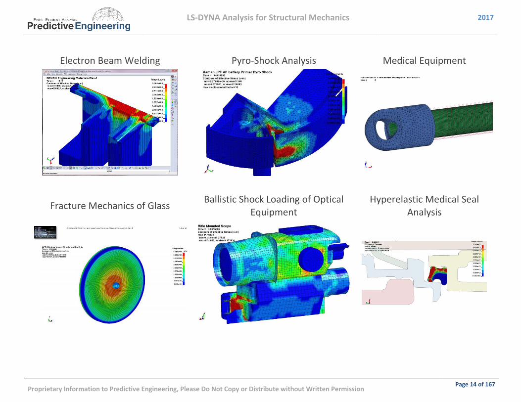
1.5 SPECIFIC APPLICATIONS (COURTESY OF PREDICTIVE ENGINEERING)
Airplane 16g Crash Analysis Sporting Goods Equipment Drop Test Consumer
Products
Drop Test of Composites / Electronics
Human Biometrics
Large Deformation of Plastics

LS-DYNA Analysis for Structural Mechanics 2017
Proprietary Information to Predictive Engineering, Please Do Not Copy or Distribute without Written Permission Page 13 of 167
Crash Analysis of Cargo Net Drop Test of Nuclear Waste
Container Impact Analysis of Foams
Plastic Thread Design PSD / Modal Analysis Digger Tooth Failure
LS-DYNA Analysis for Structural Mechanics 2017
Proprietary Information to Predictive Engineering, Please Do Not Copy or Distribute without Written Permission Page 14 of 167
Electron Beam Welding Pyro-Shock Analysis Medical Equipment
Fracture Mechanics of Glass
Ballistic Shock Loading of Optical Equipment
Hyperelastic Medical Seal Analysis

LS-DYNA Analysis for Structural Mechanics 2017
Proprietary Information to Predictive Engineering, Please Do Not Copy or Distribute without Written Permission Page 15 of 167
Blade-Out Analysis Discrete Element Method for the
Mining Industry Drop-Test of Hand Held
Electronics
Ballistic Penetration of Al/Foam Panel
High-Speed Spinning Disk Containment
Locomotive Fuel Tank

LS-DYNA Analysis for Structural Mechanics 2017
Proprietary Information to Predictive Engineering, Please Do Not Copy or Distribute without Written Permission Page 16 of 167
Crash Analysis of Bus Seats Impact Analysis of Safety Block Device
Snap-Fit Analysis – All Plastic Medical Device

LS-DYNA Analysis for Structural Mechanics 2017
Proprietary Information to Predictive Engineering, Please Do Not Copy or Distribute without Written Permission Page 17 of 167
9g Crash Analysis of Jet Engine Stand Torque Analysis of Endoscopic Medical Device
Drop, Rail Impact and PSD Analysis of Composite Container
LS-DYNA Analysis for Structural Mechanics 2017
Proprietary Information to Predictive Engineering, Please Do Not Copy or Distribute without Written Permission Page 18 of 167
2. IMPLICIT VERSUS EXPLICIT ANALYSIS
LS-DYNA is a non-linear transient dynamic finite element code with both explicit and implicit solvers.
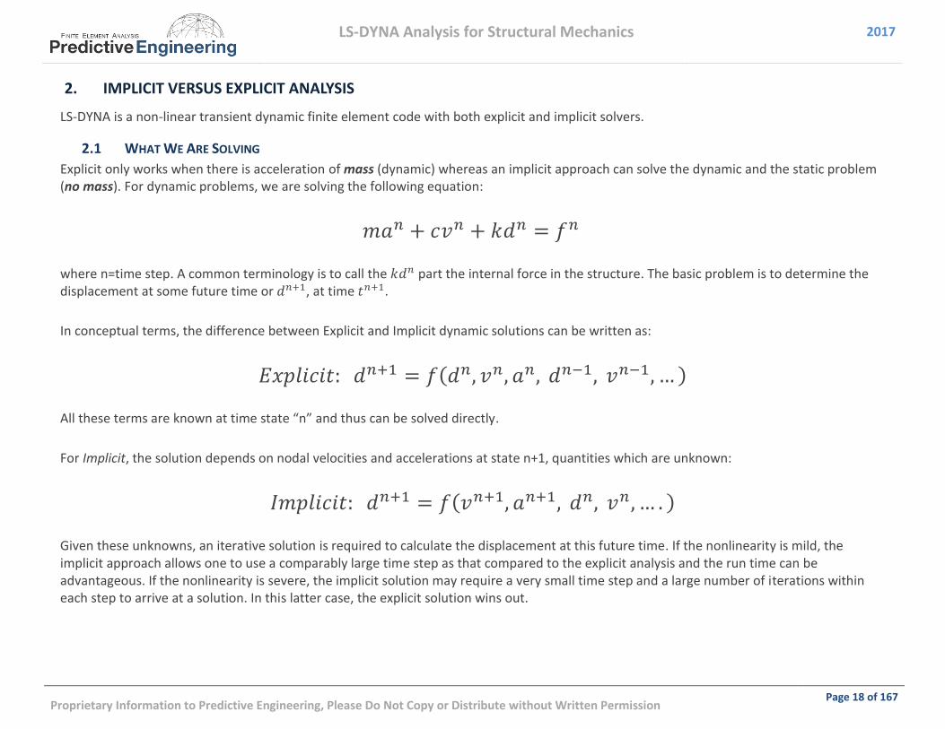
2.1 WHAT WE ARE SOLVING
Explicit only works when there is acceleration of mass (dynamic) whereas an implicit approach can solve the dynamic and the static problem (no mass). For dynamic problems, we are solving the following equation:
𝑚𝑎𝑛 + 𝑐𝑣𝑛 + 𝑘𝑑𝑛 = 𝑓𝑛
where n=time step. A common terminology is to call the 𝑘𝑑𝑛 part the internal force in the structure. The basic problem is to determine the displacement at some future time or 𝑑𝑛+1, at time 𝑡𝑛+1.
In conceptual terms, the difference between Explicit and Implicit dynamic solutions can be written as:
𝐸𝑥𝑝𝑙𝑖𝑐𝑖𝑡: 𝑑𝑛+1 = 𝑓(𝑑𝑛, 𝑣𝑛, 𝑎𝑛, 𝑑𝑛−1, 𝑣𝑛−1, … )
All these terms are known at time state “n” and thus can be solved directly.
For Implicit, the solution depends on nodal velocities and accelerations at state n+1, quantities which are unknown:
𝐼𝑚𝑝𝑙𝑖𝑐𝑖𝑡: 𝑑𝑛+1 = 𝑓(𝑣𝑛+1, 𝑎𝑛+1, 𝑑𝑛, 𝑣𝑛, … . )
Given these unknowns, an iterative solution is required to calculate the displacement at this future time. If the nonlinearity is mild, the implicit approach allows one to use a comparably large time step as that compared to the explicit analysis and the run time can be advantageous. If the nonlinearity is severe, the implicit solution may require a very small time step and a large number of iterations within each step to arrive at a solution. In this latter case, the explicit solution wins out.
LS-DYNA Analysis for Structural Mechanics 2017
Proprietary Information to Predictive Engineering, Please Do Not Copy or Distribute without Written Permission Page 19 of 167
2.2 EXPLICIT (DYNAMIC) – ONE MUST HAVE “MASS” TO MAKE IT GO
Internal and external forces are summed at each node point, and a nodal acceleration is computed by dividing by nodal mass. The solution is advanced by integrating this acceleration in time. The maximum time step size is limited by the Courant condition, producing an algorithm which typically requires many relatively inexpensive time steps. Using this criterion, the solution is unconditionally stable. Since the solution is solving for displacements at nodal points, the time step must allow the calculation to progress across the element without “skipping” nodes, that is, the time step must ensure that the stress wave stays within the element. Hence, the explicit solution is limited in time step by the element size and the speed sound in that element under study. Much more will be said about element size and the speed of sound in materials since execution speed for an explicit analysis is often of great importance given that careful meshing can mean the difference between a run time of days or hours. Just to plant the seed, but an explicit analysis is all about mass since everything has a time step (e.g., contact, 1D spring elements, CNRB’s, etc.).
2.3 IMPLICIT (DYNAMIC)
A global stiffness matrix is computed, decomposed and applied to the nodal out-of-balance force to obtain a displacement increment. Equilibrium iterations are then required to arrive at an acceptable “force balance”. The advantage of this approach is that time step size may be selected by the user. The disadvantage is the large numerical effort required to form, store, and factorize the stiffness matrix. Implicit simulations therefore typically involve a relatively small number of expensive time steps. The key point of this discussion is that the stiffness matrix (i.e., internal forces) has to be decomposed or inverted each time step whereas in the explicit method, it is a running analysis where the stiffness terms are re-computed each time step but no inversion is required. Since this numerical technique is independent of a time step approach, element size is not of direct concern only the size of the model (nodes/elements) directly affects the run time.

LS-DYNA Analysis for Structural Mechanics 2017
Proprietary Information to Predictive Engineering, Please Do Not Copy or Distribute without Written Permission Page 20 of 167
3. FUNDAMENTAL MECHANICS OF EXPLICIT ANALYSIS
3.1 TIME STEP SIGNIFICANCE

LS-DYNA Analysis for Structural Mechanics 2017
Proprietary Information to Predictive Engineering, Please Do Not Copy or Distribute without Written Permission Page 21 of 167
EXPLICIT TIME INTEGRATION 3.1.1
o Very efficient for large nonlinear problems (CPU time increases only linearly with DOF)
o No need to assemble stiffness matrix or solve system of equations
o Cost per time step is very low
o Stable time step size is limited by Courant condition (i.e., time for stress wave to traverse an element)
o Problem duration typically ranges from microseconds to tenths of seconds
o Particularly well-suited to nonlinear, high-rate dynamic problems
o Nonlinear contact/impact
o Nonlinear materials
o Finite strains/large deformations
Figure 1: How Solution Time and Result Outputs Are Defined in Explicit

LS-DYNA Analysis for Structural Mechanics 2017
Proprietary Information to Predictive Engineering, Please Do Not Copy or Distribute without Written Permission Page 22 of 167
3.2 TIME STEP SIGNIFICANCE (COURANT-FRIEDRICHS-LEWY (CFL) CHARACTERISTIC LENGTH)
• In the simplest case (small, deformation theory), the timestep is controlled by the acoustic wave propagation through the material.
• In the explicit integration, the numerical stress wave must always propagate less than one element width per timestep.
• The timestep of an explicit analysis is determined as the minimum stable timestep in any one (1) deformable finite element in the mesh. (Note: As the mesh deforms, the timestep can similarly change)
• The above relationship is called the Courant-Friedrichs-Lewy (CFL) condition and determines the stable timestep in an element. The CFL condition requires that the explicit timestep be smaller than the time needed by the physical wave to cross the element. Hence, the numerical timestep is a fraction (0.9 or lower) of the actual theoretical timestep. Note: the CFL stability proof is only possible for linear problems.
• In LS-DYNA, one can control the time step scale factor (TSSFAC). The default setting is 0.9. It is typically only necessary to change this factor for shock loading or for increased contact stability with soft materials.
𝐶𝐴𝑐𝑐𝑜𝑢𝑠𝑡𝑖𝑐𝑊𝑎𝑣𝑒𝑆𝑝𝑒𝑒𝑑 = √𝐸𝑀𝑎𝑡𝑒𝑟𝑖𝑎𝑙
𝜌𝑀𝑎𝑡𝑒𝑟𝑖𝑎𝑙
∆𝐸𝑥𝑝𝑙𝑖𝑐𝑖𝑡𝑇𝑖𝑚𝑒𝑠𝑡𝑒𝑝 =𝐿𝑒𝑛𝑔𝑡ℎ𝐸𝑙𝑒𝑚𝑒𝑛𝑡
𝐶𝑊𝑎𝑣𝑒𝑠𝑝𝑒𝑒𝑑
∆𝑇𝑖𝑚𝑠𝑡𝑒𝑝𝐶𝐹𝐿 = (0.9)∆𝐸𝑥𝑝𝑙𝑖𝑐𝑖𝑡𝑇𝑖𝑚𝑒𝑠𝑡𝑒𝑝
Analyst’s Note: Based on this conditions, the time step can be increased to provide faster solution times by artificially increasing the density of the material (e.g., mass scaling, lowering the modulus or by increasing the element size of the mesh.
LS-DYNA Analysis for Structural Mechanics 2017
Proprietary Information to Predictive Engineering, Please Do Not Copy or Distribute without Written Permission Page 23 of 167
3.3 MASS SCALING: (EVERYBODY DOES IT BUT NOBODY REALLY LIKES IT)
Explicit Time Step Mass Scaling (*Control_Timestep)*
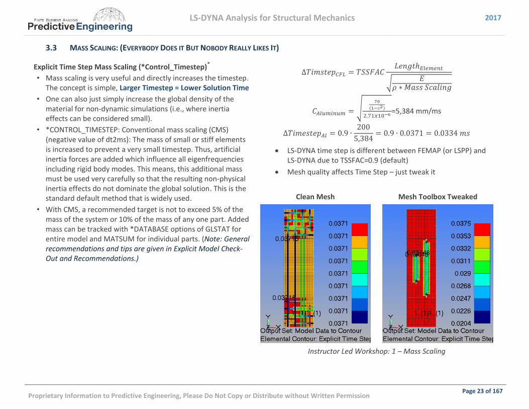
• Mass scaling is very useful and directly increases the timestep. The concept is simple, Larger Timestep = Lower Solution Time
• One can also just simply increase the global density of the material for non-dynamic simulations (i.e., where inertia effects can be considered small).
• *CONTROL_TIMESTEP: Conventional mass scaling (CMS) (negative value of dt2ms): The mass of small or stiff elements is increased to prevent a very small timestep. Thus, artificial inertia forces are added which influence all eigenfrequencies including rigid body modes. This means, this additional mass must be used very carefully so that the resulting non-physical inertia effects do not dominate the global solution. This is the standard default method that is widely used.
• With CMS, a recommended target is not to exceed 5% of the mass of the system or 10% of the mass of any one part. Added mass can be tracked with *DATABASE options of GLSTAT for entire model and MATSUM for individual parts. (Note: General recommendations and tips are given in Explicit Model Check-Out and Recommendations.)
∆𝑇𝑖𝑚𝑠𝑡𝑒𝑝𝐶𝐹𝐿 = 𝑇𝑆𝑆𝐹𝐴𝐶𝐿𝑒𝑛𝑔𝑡ℎ𝐸𝑙𝑒𝑚𝑒𝑛𝑡
√𝐸
𝜌 ∗ 𝑀𝑎𝑠𝑠 𝑆𝑐𝑎𝑙𝑖𝑛𝑔
𝐶𝐴𝑙𝑢𝑚𝑖𝑛𝑢𝑚 = √70
(1−2)
2.71𝑥10−6 =5,384 mm/ms
∆𝑇𝑖𝑚𝑒𝑠𝑡𝑒𝑝𝐴𝑙 = 0.9 ∙200
5,384= 0.9 ∙ 0.0371 = 0.0334 𝑚𝑠
LS-DYNA time step is different between FEMAP (or LSPP) and LS-DYNA due to TSSFAC=0.9 (default)
Mesh quality affects Time Step – just tweak it
Clean Mesh Mesh Toolbox Tweaked
Instructor Led Workshop: 1 – Mass Scaling
LS-DYNA Analysis for Structural Mechanics 2017
Proprietary Information to Predictive Engineering, Please Do Not Copy or Distribute without Written Permission Page 24 of 167
WORKSHOP: 1 - LS-DYNA MASS SCALING BASICS 3.3.1
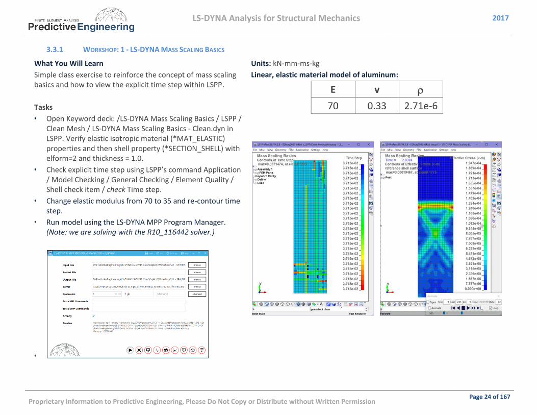
What You Will Learn
Simple class exercise to reinforce the concept of mass scaling basics and how to view the explicit time step within LSPP.
Tasks
• Open Keyword deck: /LS-DYNA Mass Scaling Basics / LSPP / Clean Mesh / LS-DYNA Mass Scaling Basics - Clean.dyn in LSPP. Verify elastic isotropic material (*MAT_ELASTIC) properties and then shell property (*SECTION_SHELL) with elform=2 and thickness = 1.0.
• Check explicit time step using LSPP’s command Application / Model Checking / General Checking / Element Quality / Shell check item / check Time step.
• Change elastic modulus from 70 to 35 and re-contour time step.
• Run model using the LS-DYNA MPP Program Manager. (Note: we are solving with the R10_116442 solver.)
•
Units: kN-mm-ms-kg
Linear, elastic material model of aluminum:
E v
70 0.33 2.71e-6

LS-DYNA Analysis for Structural Mechanics 2017
Proprietary Information to Predictive Engineering, Please Do Not Copy or Distribute without Written Permission Page 25 of 167
Workshop: 1 – LS-DYNA Mass Scaling Basics (continued)
With the model working, let’s harvest some data. We are going to make several runs of this model to investigate the relationship between mesh, explicit time step and mass scaling. As part of this process, you’ll get comfortable working with LSPP and LS-DYNA MPP Program Manager. Our metric is going to be the maximum displacement from a node at the end of the bar.
Tasks
• Within existing LSPP model, open History, select Node, Y-Displacement and then pick a node at the very top of the bar near the center (any’ol node near the center) and then likewise at the bottom, near the center. When done you should have two nodes selected and then hit Plot within the History dialog box. When finished something like this should appear as a graph.
• Note that the maximum displacement at the top of the bar is 0.00684 mm.
Objective
Open the Keyword Deck LS-DYNA Mass Scaling Basics - Skewed Mesh - Start.dyn in your favorite text editor and apply conventional mass scaling (CMS) to the *CONTROL_TIMESTEP keyword card via the dt2ms option. The idea is to match the original time step in the clean mesh example.
(Note: Remember that the tssfac=0.9 and thus to get an explicit step of 1.0, one must use a value of dt2ms=-1.111.)
Model Time Step % Mass Added by Mass Scaling Max. Displacement
Starting Point 0.0334 ms 0.00% 0.00684 mm
Skewed Mesh (-4x) 0.0184 ms 0.00% mm
Skewed Mesh with Mass Scaling 0.0334 ms 16.9% mm
LS-DYNA Analysis for Structural Mechanics 2017
Proprietary Information to Predictive Engineering, Please Do Not Copy or Distribute without Written Permission Page 26 of 167
INSTRUCTOR LED WORKSHOP: 2 - MASS SCALING ADVANCED 3.3.2
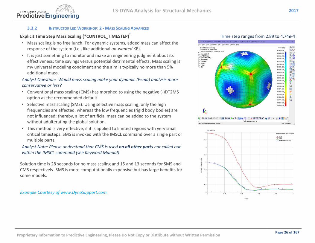
Explicit Time Step Mass Scaling (*CONTROL_TIMESTEP)*
• Mass scaling is no free lunch. For dynamic systems, added mass can affect the response of the system (i.e., like additional un-wanted KE).
• It is just something to monitor and make an engineering judgment about its effectiveness; time savings versus potential detrimental effects. Mass scaling is my universal modeling condiment and the aim is typically no more than 5% additional mass.
Analyst Question: Would mass scaling make your dynamic (F=ma) analysis more conservative or less?
• Conventional mass scaling (CMS) has morphed to using the negative (-)DT2MS option as the recommended default.
• Selective mass scaling (SMS): Using selective mass scaling, only the high frequencies are affected, whereas the low frequencies (rigid body bodies) are not influenced; thereby, a lot of artificial mass can be added to the system without adulterating the global solution.
• This method is very effective, if it is applied to limited regions with very small critical timesteps. SMS is invoked with the IMSCL command over a single part or multiple parts.
Analyst Note: Please understand that CMS is used on all other parts not called out within the IMSCL command (see Keyword Manual)
Solution time is 28 seconds for no mass scaling and 15 and 13 seconds for SMS and CMS respectively. SMS is more computationally expensive but has large benefits for some models.
Time step ranges from 2.89 to 4.74e-4
Example Courtesy of www.DynaSupport.com
LS-DYNA Analysis for Structural Mechanics 2017
Proprietary Information to Predictive Engineering, Please Do Not Copy or Distribute without Written Permission Page 27 of 167
3.4 IMPLICIT MESH VERSUS EXPLICIT MESH CHARACTERISTICS
INSTRUCTOR LED WORKSHOP: 3 - IMPLICIT VERSUS EXPLICIT MESH DIFFERENCES 3.4.1
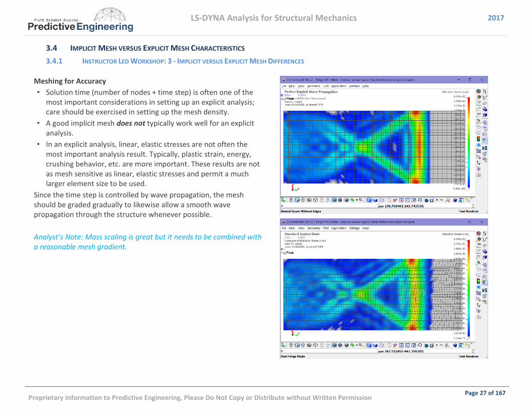
Meshing for Accuracy
• Solution time (number of nodes + time step) is often one of the most important considerations in setting up an explicit analysis; care should be exercised in setting up the mesh density.
• A good implicit mesh does not typically work well for an explicit analysis.
• In an explicit analysis, linear, elastic stresses are not often the most important analysis result. Typically, plastic strain, energy, crushing behavior, etc. are more important. These results are not as mesh sensitive as linear, elastic stresses and permit a much larger element size to be used.
Since the time step is controlled by wave propagation, the mesh should be graded gradually to likewise allow a smooth wave propagation through the structure whenever possible.
Analyst’s Note: Mass scaling is great but it needs to be combined with a reasonable mesh gradient.
LS-DYNA Analysis for Structural Mechanics 2017
Proprietary Information to Predictive Engineering, Please Do Not Copy or Distribute without Written Permission Page 28 of 167
4. LS-DYNA GETTING STARTED WITH THE FUNDAMENTALS
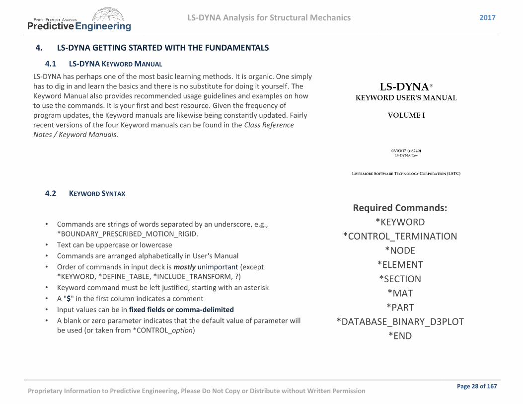
4.1 LS-DYNA KEYWORD MANUAL
LS-DYNA has perhaps one of the most basic learning methods. It is organic. One simply has to dig in and learn the basics and there is no substitute for doing it yourself. The Keyword Manual also provides recommended usage guidelines and examples on how to use the commands. It is your first and best resource. Given the frequency of program updates, the Keyword manuals are likewise being constantly updated. Fairly recent versions of the four Keyword manuals can be found in the Class Reference Notes / Keyword Manuals.
4.2 KEYWORD SYNTAX
• Commands are strings of words separated by an underscore, e.g., *BOUNDARY_PRESCRIBED_MOTION_RIGID.
• Text can be uppercase or lowercase
• Commands are arranged alphabetically in User's Manual
• Order of commands in input deck is mostly unimportant (except *KEYWORD, *DEFINE_TABLE, *INCLUDE_TRANSFORM, ?)
• Keyword command must be left justified, starting with an asterisk
• A "$" in the first column indicates a comment
• Input values can be in fixed fields or comma-delimited
• A blank or zero parameter indicates that the default value of parameter will be used (or taken from *CONTROL_option)
Required Commands:
*KEYWORD
*CONTROL_TERMINATION
*NODE
*ELEMENT
*SECTION
*MAT
*PART
*DATABASE_BINARY_D3PLOT
*END

LS-DYNA Analysis for Structural Mechanics 2017
Proprietary Information to Predictive Engineering, Please Do Not Copy or Distribute without Written Permission Page 29 of 167
4.3 UNITS
Many a fine analysis model has been brought down by bad units. Although one may wonder why in this modern age one still has to twiddle with units and not have it addressed by the interface is philosophical-like engineering debate between the ability to hand-edit the “deck” or be hand-cuffed to a gui (pronounced “gooey”) interface. Moving past this discussion, to use LS-DYNA effectively, one should have a rock-solid and un-shakable conviction in your chosen system of units.
Since the majority of LS-DYNA work is dynamic, the analyst will often be looking at the energies of the system or velocities, in addition to displacements and stresses. Hence, a consistent set of units that are easy to follow can provide significant relief in the debugging of an errant analysis. A general guide to units can be viewed within the Class Reference Notes / Units (see Consistent units — LS-DYNA Support.pdf). Saying all that, here are the four unit systems that I have standardized on for analysis work. It doesn’t mean they are the best but at least they are generally accepted.
Consistent Unit Sets for LS-DYNA Analysis
Mass Length Time Force Stress Energy Density Steel Young’s Gravity
kg m s N Pa J 7,800 2.07e+9 9.806
g mm ms N MPa N-mm 7.83e-03 2.07e+05 9.806e-03
Ton (1,000 kg) mm s N MPa N-mm 7.83e-09 2.07e+05 9.806e+03
Lbf-s2/in (snail) in s lbf psi lbf-in 7.33e-04 3.00e+07 386

LS-DYNA Analysis for Structural Mechanics 2017
Proprietary Information to Predictive Engineering, Please Do Not Copy or Distribute without Written Permission Page 30 of 167
4.4 REFERENCE MATERIALS AND PROGRAM DOWNLOAD
The first site to visit: www.lsdynasupport.com
Another great site: www.dynasupport.com
LS-DYNA Examples: www.DYNAExamples.com
LS-DYNA Conference Papers: www.dynalook.com
Newsletter: www.FEAInformation.com
Newsletter and Seminars: www.DYNAmore.com
Yahoo Discussion Group: [email protected]
Aerospace Working Group: awg.lstc.com
Varmit Al’s Material Database (google’it)
LSTC Program Download Site ftp://user:[email protected]
SMP Version: ls-dyna
MPP Version: mpp-dyna
SMP/Windows: pc-dyna
For Development Programs:
ftp://beta:[email protected]
INTERNAL LSTC FAQ - FTP://FTP.LSTC.COM/OUTGOING/SUPPORT/FAQ 4.4.1
LS-DYNA Analysis for Structural Mechanics 2017
Proprietary Information to Predictive Engineering, Please Do Not Copy or Distribute without Written Permission Page 31 of 167
4.5 SUBMITTING LS-DYNA ANALYSIS JOBS AND SENSE SWITCHES
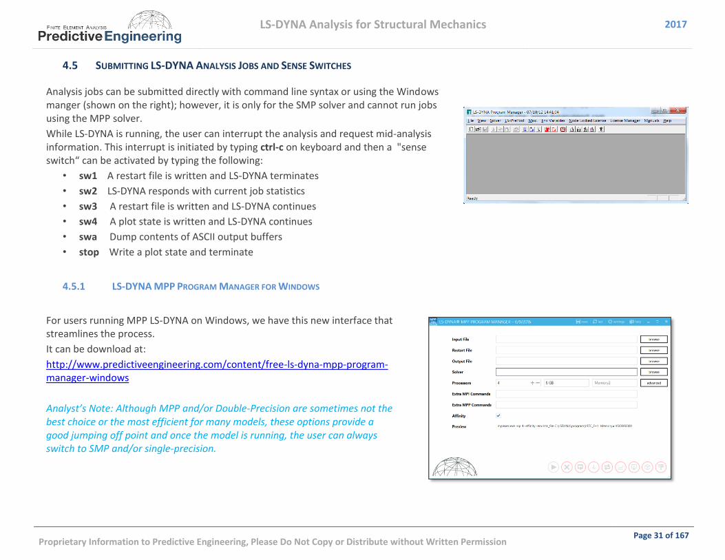
Analysis jobs can be submitted directly with command line syntax or using the Windows manger (shown on the right); however, it is only for the SMP solver and cannot run jobs using the MPP solver.
While LS-DYNA is running, the user can interrupt the analysis and request mid-analysis information. This interrupt is initiated by typing ctrl-c on keyboard and then a "sense switch“ can be activated by typing the following:
• sw1 A restart file is written and LS-DYNA terminates
• sw2 LS-DYNA responds with current job statistics
• sw3 A restart file is written and LS-DYNA continues
• sw4 A plot state is written and LS-DYNA continues
• swa Dump contents of ASCII output buffers
• stop Write a plot state and terminate
LS-DYNA MPP PROGRAM MANAGER FOR WINDOWS 4.5.1
For users running MPP LS-DYNA on Windows, we have this new interface that streamlines the process.
It can be download at:
http://www.predictiveengineering.com/content/free-ls-dyna-mpp-program-manager-windows
Analyst’s Note: Although MPP and/or Double-Precision are sometimes not the best choice or the most efficient for many models, these options provide a good jumping off point and once the model is running, the user can always switch to SMP and/or single-precision.
LS-DYNA Analysis for Structural Mechanics 2017
Proprietary Information to Predictive Engineering, Please Do Not Copy or Distribute without Written Permission Page 32 of 167
4.6 WORKSHOP: 2 - LS-DYNA GETTING STARTED
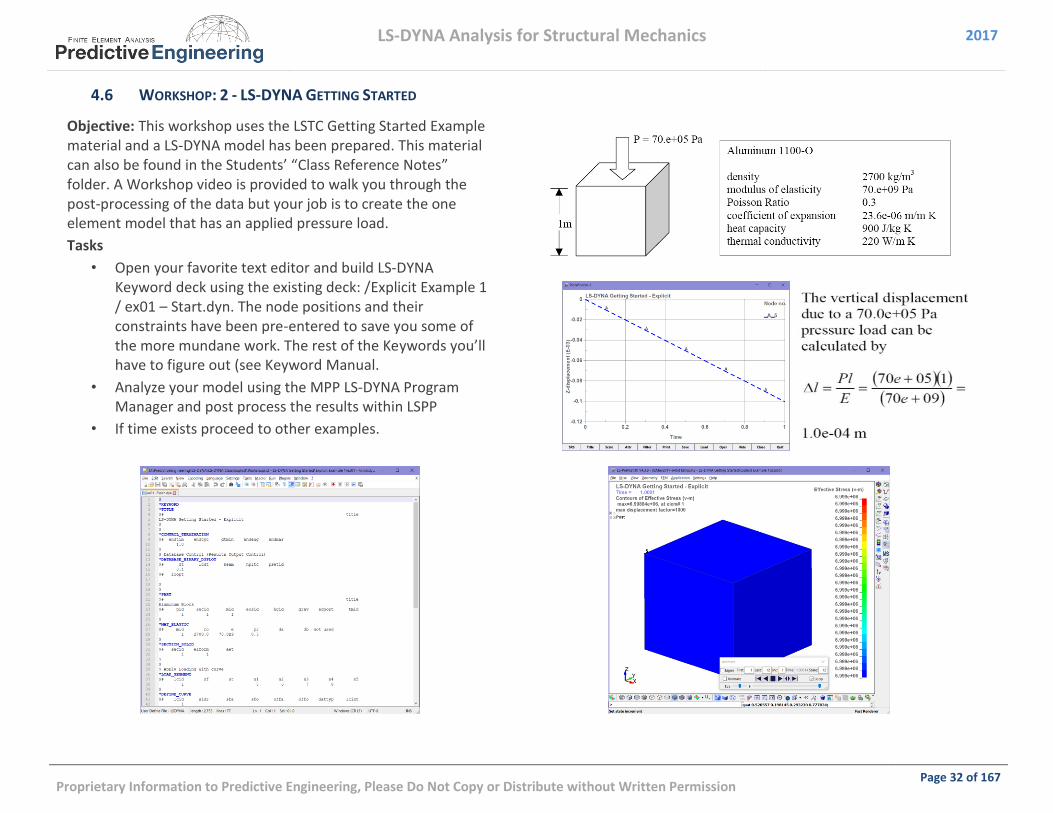
Objective: This workshop uses the LSTC Getting Started Example material and a LS-DYNA model has been prepared. This material can also be found in the Students’ “Class Reference Notes” folder. A Workshop video is provided to walk you through the post-processing of the data but your job is to create the one element model that has an applied pressure load.
Tasks
• Open your favorite text editor and build LS-DYNA Keyword deck using the existing deck: /Explicit Example 1 / ex01 – Start.dyn. The node positions and their constraints have been pre-entered to save you some of the more mundane work. The rest of the Keywords you’ll have to figure out (see Keyword Manual.
• Analyze your model using the MPP LS-DYNA Program Manager and post process the results within LSPP
• If time exists proceed to other examples.
LS-DYNA Analysis for Structural Mechanics 2017
Proprietary Information to Predictive Engineering, Please Do Not Copy or Distribute without Written Permission Page 33 of 167
5. EXPLICIT ELEMENT TECHNOLOGY
5.1 ELEMENT TYPES IN LS-DYNA
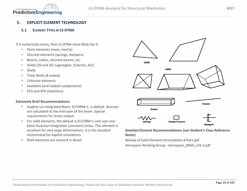
If it numerically exists, then LS-DYNA most likely has it:
• Point elements (mass, inertia)
• Discrete elements (springs, dampers)
• Beams, cables, discrete-beams, etc.
• Solids (20 and 3D, Lagrangian, Eulerian, ALE)
• Shells
• Thick Shells (8 noded)
• Cohesive elements
• Seatbelts (and related components)
• EFG and SPH (meshless)
Extremely Brief Recommendations
• Hughes-Liu Integrated Beam, ELFORM=1, is default. Stresses are calculated at the mid-span of the beam. Special requirements for stress output.
• For solid elements, the default is ELFORM=1 and uses one-point Guassian Integration (constant) stress. This element is excellent for very large deformations. It is the standard recommend for explicit simulations.
• Shell elements are covered in detail.
Detailed Element Recommendations (see Student’s Class Reference Notes)
Review of Solid Element Formulations Erhart.pdf
Aerospace Working Group - Aerospace_MGD_v16-2.pdf
LS-DYNA Analysis for Structural Mechanics 2017
Proprietary Information to Predictive Engineering, Please Do Not Copy or Distribute without Written Permission Page 81 of 167
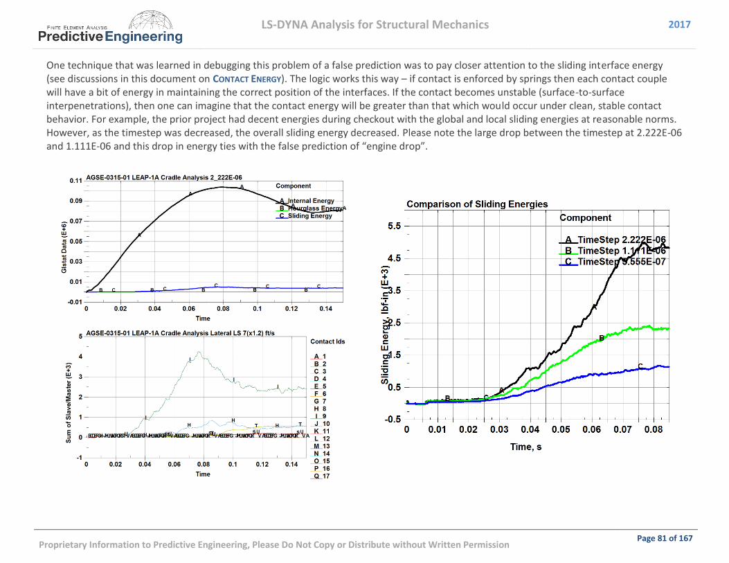
One technique that was learned in debugging this problem of a false prediction was to pay closer attention to the sliding interface energy (see discussions in this document on CONTACT ENERGY). The logic works this way – if contact is enforced by springs then each contact couple will have a bit of energy in maintaining the correct position of the interfaces. If the contact becomes unstable (surface-to-surface interpenetrations), then one can imagine that the contact energy will be greater than that which would occur under clean, stable contact behavior. For example, the prior project had decent energies during checkout with the global and local sliding energies at reasonable norms. However, as the timestep was decreased, the overall sliding energy decreased. Please note the large drop between the timestep at 2.222E-06 and 1.111E-06 and this drop in energy ties with the false prediction of “engine drop”.

LS-DYNA Analysis for Structural Mechanics 2017
Proprietary Information to Predictive Engineering, Please Do Not Copy or Distribute without Written Permission Page 82 of 167
8.7 CONTACT BEST PRACTICES
Recommendation Why
_AUTOMATIC_SINGLE_SURFACE_MORTAR It is the most robust and _SINGLE_SURFACE as a default will track penetrations and slowly remove them. Once your explicit simulation is stable, one can always remove _MORTAR later on for a speed improvement.
_AUTOMATIC_SURFACE_TO_SURFACE_MORTAR
If high negative sliding interface energy is noted, it is useful to break up your contacts into part-to-part or {part set}-to-{part set} via SURFACE_TO_SURFACE to pinpoint the contact region that is causing problems.
_AUTOMATIC_SINGLE or SURFACE_TO_SURFACE w/soft=2 This is our recommended backup if greater numerical efficiency is required. The soft=2 option on the optional A card switches the contact formulation to a segment base and adjusts the contact stiffness for better contact.
Check your model for penetrations (LSPP – Application / Model Checking / General Checking / Contact Check). Keep in mind that _MORTAR, as a default, automatically accommodates small penetrations.
Be aware of their magnitude since they contribute to negative sliding interface energy, poor contact behavior and spurious contact forces.
For contact between deformable bodies, aim for a uniform mesh pattern.
Contact works by segments and transfers contact forces to the adjacent nodes. If the mesh is course, the contact forces will be high and dynamic. The smoother the patter the better the contact.

LS-DYNA Analysis for Structural Mechanics 2017
Proprietary Information to Predictive Engineering, Please Do Not Copy or Distribute without Written Permission Page 83 of 167
8.8 MESH TRANSITIONS: TIED CONTACT FOR WELDING AND GLUING
TIED CONTACT OR GLUING 8.8.1
Given the idealization difficulty of system modeling, the ability to tie together different mesh densities (e.g., hex-to-hex or tet-to-hex), snap together parts along a weld-line or just glue sections together (e.g., plate edge to a solid mesh) is an amazingly useful ability and LS-DYNA provides a very complete Tied Contact tool box to work with.
The emphasis of this course to provide an overview of the basics to get started efficiently with LS-DYNA, a short list of recommended *KEYWORDS for Tied Contact are presented that work for both implicit and explicit solution sequences.
When the Mesh is Co-Planar (Translational DOF Tied)
• *CONTACT_TIED_SURFACE_TO_SURFACE
• *CONTACT_TIED_NODES_TO_SURFACE
When the Mesh is Co-Planar (All Six DOF Tied)
• *CONTACT_TIED_SHELL_EDGE_TO_SURFACE
When the Mesh is Offset (All Six DOF Tied)
• *CONTACT_TIED_SURFACE_TO_SURFACE_BEAM_OFFSET
• *CONTACT_TIED_SHELL_EDGE_TO_SURFACE_BEAM_OFFSET
The utility of using a very brief subset is that one can build up experience and confidence without the expense of trying out a rather daunting list of Tied Contact Options.
Analyst’s Note: Tied contacts are not really “contacts” but a constraint or penalty relationship that uses the *CONTACT card entry format. For an explicit analysis, the constraint option ties the slave to the master accelerations (see Theory Manual) while for implicit, the displacements are tied. This explains why the nodes must be on the same plane and also why this formulation can’t be used with rigid bodies or have SPCs attached to any node that is tied. Additionally, it is only generally applicable for just translational DOF (TX, TY & TZ).
With the OFFSET formulation, the penalty method is used. If the BEAM option is employed all six DOF’s are tied together by essentially using little springs between the nodes. This is the most computationally expensive tied contact but the most robust. Since the tied contact is enforced by springs, the nodes can be offset, rigid bodies can be tied together and even SPCs can be applied to the tied interface nodes.
The reason that we like default Tied (constraint) contact is
that it is stable whereas penalty Tied Contact _Offset is penalty based and has all the standard pathologies of regular contact such as the possibility of creating negative sliding interface energy.
LS-DYNA Analysis for Structural Mechanics 2017
Proprietary Information to Predictive Engineering, Please Do Not Copy or Distribute without Written Permission Page 84 of 167
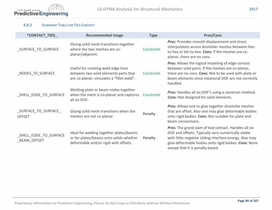
SUMMARY TABLE FOR TIED CONTACT 8.8.2
*CONTACT_TIED_ Recommended Usage Type Pros/Cons
_SURFACE_TO_SURFACE Gluing solid mesh transitions together where the two meshes are co-planar/adjacent.
Constraint
Pros: Provides smooth displacement and stress interpolation across dissimilar meshes between hex-to-hex or tet-to-hex. Cons: If the meshes are co-planar, there are no cons.
_NODES_T0_SURFACE Useful for creating weld edge lines between two solid elements parts that are co-planar; simulates a “fillet weld”.
Constraint
Pros: Allows the logical modeling of edge contact between solid parts. If the meshes are co-planar, there are no cons. Cons: Not to be used with plate or beam elements since rotational DOF are not correctly handled.
_SHELL_EDGE_TO_SURFACE Welding plate or beam nodes together when the mesh is co-planar and captures all six DOF.
Constraint Pros: Handles all six DOF’s using a constrain method. Cons: Not designed for solid elements.
_SURFACE_TO_SURFACE_
OFFSET
Gluing solid mesh transitions when the meshes are not co-planar.
Penalty
Pros: Allows one to glue together dissimilar meshes that are offset. Also one may glue deformable bodies onto rigid bodies. Cons: Not suitable for plate and beam connections.
_SHELL_EDGE_TO_SURFACE_BEAM_OFFSET
Ideal for welding together plates/beams or for plates/beams onto solids whether deformable and/or rigid with offsets.
Penalty
Pros: The grand slam of tied contact. Handles all six DOF and offsets. Typically very numerically stable with little negative sliding interface energy. Also may glue deformable bodies onto rigid bodies. Cons: None except that it is penalty based.

LS-DYNA Analysis for Structural Mechanics 2017
Proprietary Information to Predictive Engineering, Please Do Not Copy or Distribute without Written Permission Page 85 of 167
WORKSHOP: 15 - TIED CONTACT FOR HEX-TO-TET MESH TRANSITIONS (TIED_SURFACE_TO_SURFACE) 8.8.3
Background for TIED Contact Analysis
The advantages of using a hex mesh for explicit work centers on better shape control during large deformation and the ability to maintain a larger time step. The last items is often pivotal in keeping your solution running fast without having the program add excessive mass if automatic mass scaling is invoked (*CONTROL_TIMESTEP (DTMS = negative timestep value)). In the implicit world, the use of hex elements are desired for the ability to provide equivalent stress mapping using far less nodes (eight node brick versus the use of five 10-node tetrahedrals to fill the same space or 8/26 nodes) and often times, cleaner stress contours. This workshop shows how to setup the mesh transition and run the analysis using the implicit solution.
Tasks
▫ Start with opening up the Keyword deck: Tied Contact - Mesh Transition Hex to Tet - Start.dyn and inspect the Keywords. It is setup for an explicit run. Input the settings required to enable _TIED_SURFACE_TO_SURFACE. Our recommendation is by *PART id.
▫ Run model and wait for it to finish. Better idea, apply CMS. What value? Open model in LSPP and assess the time step Application / Model Checking / etc. Apply reasonable value of -2d2ms that will give you something under <10% mass scaling. Run model.
▫ Inspect model, check applied force (plot SPCFORC) and look at ratio of kinetic/internal energy. Is the model at equilibrium?
▫ Time to clean up the model. Inspect mess0000 file and notice warnings. To fix this, we’ll create a segment set in LSPP for the slave side of the _TIED contact such that only nodes close to the interface will be part of the slave set. Reconfigure the _TIED card to use segment set and rerun. Done.
Analyst’s Note: The prior model was run as implicit (see folder Implicit) and if one finishes the prior workshop
quickly, one can inspect the Keyword deck and learn a bit more about implicit.

LS-DYNA Analysis for Structural Mechanics 2017
Proprietary Information to Predictive Engineering, Please Do Not Copy or Distribute without Written Permission Page 86 of 167
WORKSHOP: 16 - TIED CONTACT FOR GLUING THINGS TOGETHER (BEAM_OFFSET) 8.8.4
Objective: To understand how tied contact can easily glue structures together that are not coincident. There is much to learn and there are limitations. But if one understands the theory, it leads to confidence in how the tying or gluing is done.
Tasks
o Open up the start file: Tied Contact - Gluing Things Together - Start.dyn. It is set up to run minus the _TIED contact definition. That is your job. There is a predefined slave node set and one can use the Part id for the master side definition. Since it is shells with six dof and the surface is offset, these hints should lead you to choose the correct _TIED setup. The real question is whether one uses the _OFFSET method or the plain vanilla non-offset method?
o For Curiosity, use a non-offset method and see what happens to the slave side. Then reset the _TIED contact method and use an _OFFSET method. The – Finish _OFFSET and – Finish non-offset are both setup to provide guidance if your intuition and research fails you.
Non-offset: slave nodes are moved to master surface (if within reach, if not one can set sst and mst to a negative number that reaches)
_OFFSET: does not move slave nodes but they have to be in reach.
o With Any luck, you’ll see something like this when you are done.
Analyst’s Note: The Tied option considers a node “tied” if it is within 5% of the element’s thickness. This applies to all _TIED formulations. As mentioned, the constraint option moves the slave node to be adjacent to the master surface while the offset option accounts for the gap; but whether or not it is tied, depends upon the separation of the nodes. To override the default setting, one can set the SST to a negative number that reflects the absolute distance to search for a tie relationship between the slave and master nodes.
LS-DYNA Analysis for Structural Mechanics 2017
Proprietary Information to Predictive Engineering, Please Do Not Copy or Distribute without Written Permission Page 87 of 167
MESH TRANSITIONS: MASTERING TIED CONTACT (STUDENT EXTRA CREDIT) 8.8.5
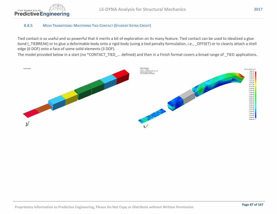
Tied contact is so useful and so powerful that it merits a bit of exploration on its many feature. Tied contact can be used to idealized a glue bond (_TIEBREAK) or to glue a deformable body onto a rigid body (using a tied penalty formulation, i.e., _OFFSET) or to cleanly attach a shell edge (6 DOF) onto a face of some solid elements (3 DOF).
The model provided below in a start (no *CONTACT_TIED_... defined) and then in a Finish format covers a broad range of _TIED applications.

LS-DYNA Analysis for Structural Mechanics 2017
Proprietary Information to Predictive Engineering, Please Do Not Copy or Distribute without Written Permission Page 88 of 167
INSTRUCTOR LED WORKSHOP: 6 - _TIED BAD ENERGY (OR WHY WE USE _BEAM_OFFSET) 8.8.6
If anything this little dialog is to remind myself to be careful with Tied Contact’s with “OFFSET”. As mentioned, the Offset option indicates that the algorithm is using the penalty method to enforce the locked motion between parts. When there is “penalty” one has the opportunity to create negative sliding interface energy since springs are used to enforce the locked positions. This behavior killed a rather simple analysis. It was a bit amazing how it completely changed the behavior of the structure. The fix is just to change the contact to _BEAM_OFFSET.
The two models are provided. Which model is right? {on the full model it was a complete FUBAR}
Analyst’s Note: Why din’t we just use _BEAM_OFFSET as the default? It was an inherited model and I wasn’t quite aware that _BEAM_OFFSET is the recommended go-forward formulation by LSTC and hey, how could a _TIED contact kill your model anyway?. It pays to understand your craft and stay abreast of new developments since this problem cost me a couple of days.
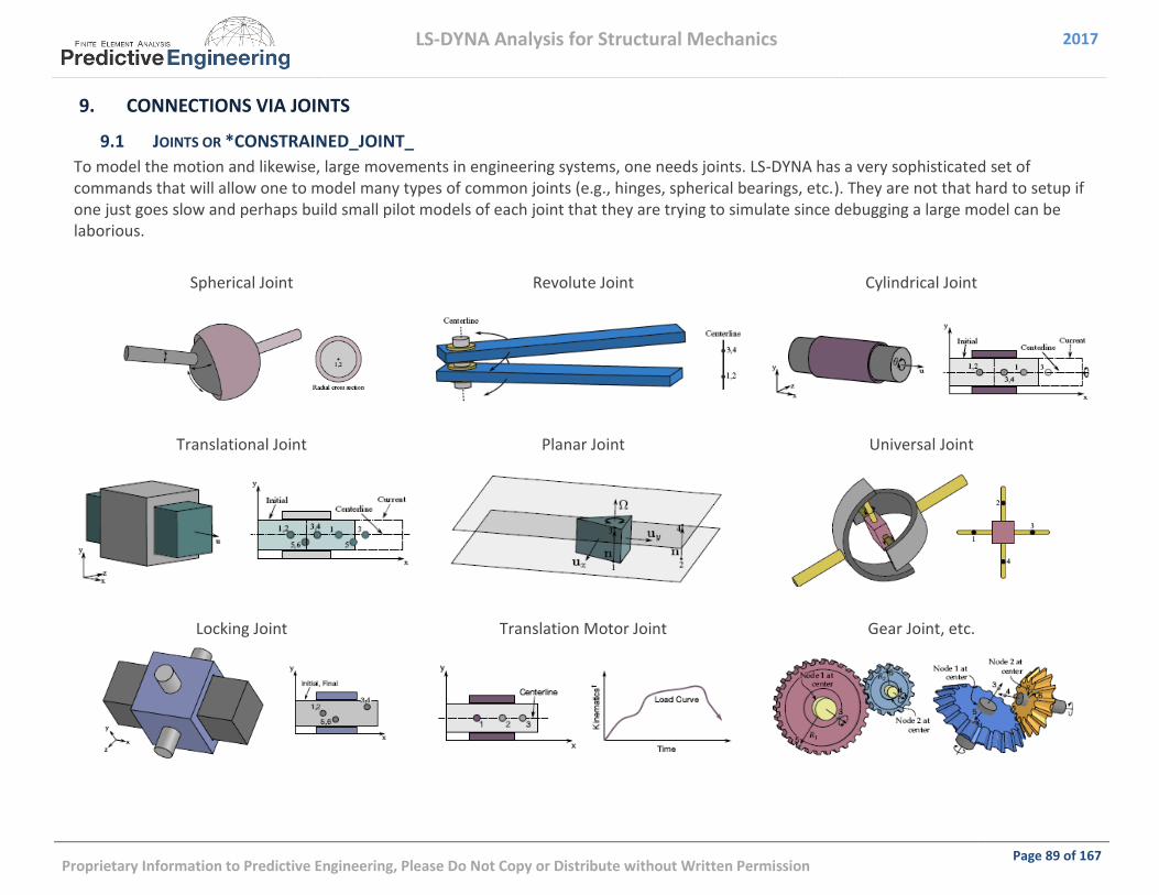
LS-DYNA Analysis for Structural Mechanics 2017
Proprietary Information to Predictive Engineering, Please Do Not Copy or Distribute without Written Permission Page 89 of 167
9. CONNECTIONS VIA JOINTS
9.1 JOINTS OR *CONSTRAINED_JOINT_
To model the motion and likewise, large movements in engineering systems, one needs joints. LS-DYNA has a very sophisticated set of commands that will allow one to model many types of common joints (e.g., hinges, spherical bearings, etc.). They are not that hard to setup if one just goes slow and perhaps build small pilot models of each joint that they are trying to simulate since debugging a large model can be laborious.
Spherical Joint Revolute Joint Cylindrical Joint
Translational Joint Planar Joint Universal Joint
Locking Joint Translation Motor Joint Gear Joint, etc.

LS-DYNA Analysis for Structural Mechanics 2017
Proprietary Information to Predictive Engineering, Please Do Not Copy or Distribute without Written Permission Page 90 of 167
9.2 HOW JOINTS WORK
The foundation of joints lie in the use of *CONSTRAINED_NODAL_RIGID_BODIES (CNRB) to provide the framework for the action of the joints.
The joint mechanical behavior is implemented using the penality method (i.e., like contact). As such, a joint has a stiffness and energy. The
stiffness of the joint is calculated based on more math that I want to describe in this brief note (Please see LS-DYNA Theory Manual
2014 for the complete description) what is directly of importance is that the joint stiffness is based on the mass of the joint’s CNRB and
their geometry, and that the reaction forces to enforce the joint’s behavior, are applied at the center-of-mass of the CNRB.
Analyst’s Note: Given that joints use the penality method, one can have joint failure (i.e., unexpectively flying apart) by using CNRB’s with too little mass and having the opposing CNRB’s center-of-mass to close to resist displacements/moments. One may want to read the Keyword *CONTROL_RIGID for some interesting notes on CNRB w.r.t. joints and mass scaling.
The simplest joint is the spherical joint which connects two
coincident nodes between two CNRB’s. A more interesting
joint is the *CONSTRAINED_JOINT_CYLINDRICAL which
requires two colinear nodes within the opposing CNRB’s.
Please note that the node sets are separated by some
reasonable distance to ensure that the joint doesn’t “blow-
up”. What is reasonable? It depends on the mass of the
CNRB’s and the magnitude of the force that is applied to
the joint. If this joint is expected to receive a high bending
load (MZ), then it would be good to ensure a large
separation between the node sets. There are no hard
guidelines but the reality is that most joints function just fine.
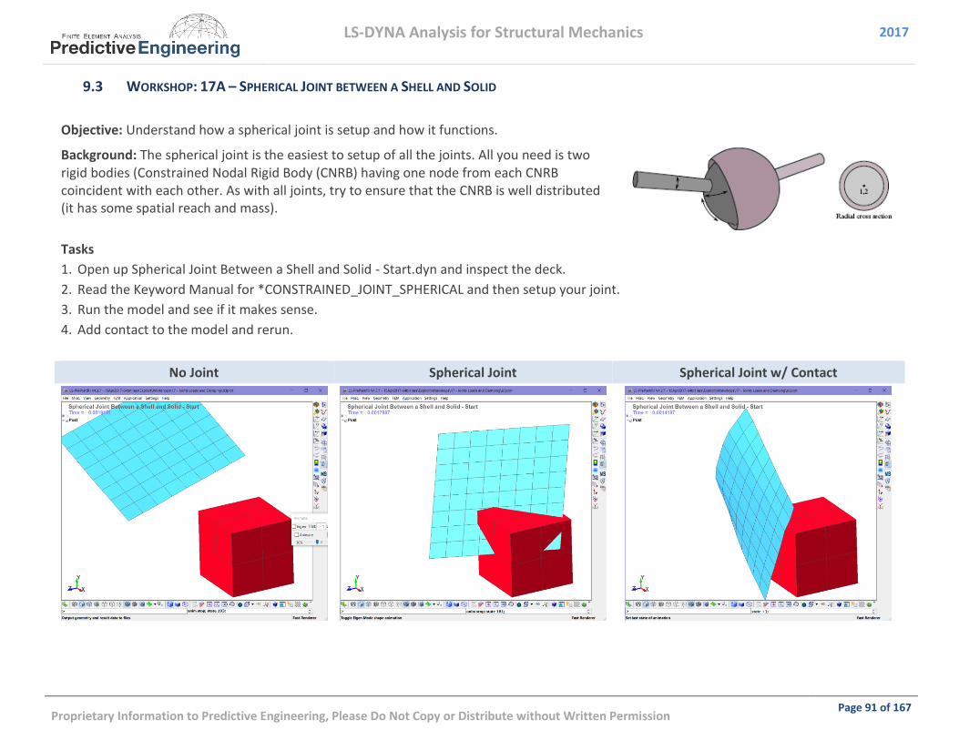
LS-DYNA Analysis for Structural Mechanics 2017
Proprietary Information to Predictive Engineering, Please Do Not Copy or Distribute without Written Permission Page 91 of 167
9.3 WORKSHOP: 17A – SPHERICAL JOINT BETWEEN A SHELL AND SOLID
Objective: Understand how a spherical joint is setup and how it functions.
Background: The spherical joint is the easiest to setup of all the joints. All you need is two rigid bodies (Constrained Nodal Rigid Body (CNRB) having one node from each CNRB coincident with each other. As with all joints, try to ensure that the CNRB is well distributed (it has some spatial reach and mass).
Tasks
1. Open up Spherical Joint Between a Shell and Solid - Start.dyn and inspect the deck.
2. Read the Keyword Manual for *CONSTRAINED_JOINT_SPHERICAL and then setup your joint.
3. Run the model and see if it makes sense.
4. Add contact to the model and rerun.
No Joint Spherical Joint Spherical Joint w/ Contact

LS-DYNA Analysis for Structural Mechanics 2017
Proprietary Information to Predictive Engineering, Please Do Not Copy or Distribute without Written Permission Page 92 of 167
9.4 WORKSHOP: 17B - CYLINDRICAL JOINT BETWEEN TWO NESTED CYLINDERS
Objective: Understand how a spherical joint is setup and how it functions.
Background: The spherical joint is the easiest to setup of all the joints. All you need is two rigid bodies (Constrained Nodal Rigid Body (CNRB) having one node from each CNRB coincident with each other. As with all joints, try to ensure that the CNRB is well distributed (it has some spatial reach and mass).
Tasks
5. Open up Cylindrical Joint Between Two Cylinders - Start.dyn and inspect the deck.
6. Read the Keyword Manual for *CONSTRAINED_JOINT_CYLINDRICAL and then setup your joint.
7. Run the model and see if it makes sense.
8. Add contact to the model and rerun. Notice how *CONTACT is setup, change sfs=1 (default) and rerun.
Cylindrical Joint w/Whipping Beam Contact

LS-DYNA Analysis for Structural Mechanics 2017
Proprietary Information to Predictive Engineering, Please Do Not Copy or Distribute without Written Permission Page 93 of 167
WHO USES JOINTS? 9.4.1
Background: Joints are very prevalent in seat analysis and automotive simulation. One could spend days working on joint setup and our only comment is that they do work if one is careful with the setup.

LS-DYNA Analysis for Structural Mechanics 2017
Proprietary Information to Predictive Engineering, Please Do Not Copy or Distribute without Written Permission Page 133 of 167
18.5.1.1 Keywords Used in this Section for Solid Elements
The practice going forward is only to mention Keywords that are unique to the implicit analysis procedure and it is assumed that the reader is familiar with the standard Keywords to run an explicit analysis. For example, the Keyword *CONTROL_TERMINATION is not discussed although it is required to run the analysis.
Keyword Card Variable Description
*CONTROL_IMPLICIT_GENERAL IMFLAG=1 & DTO=1.0 This is where we start by telling LS-DYNA that an implicit analysis is being requested.
*CONTROL_IMPLICIT_SOLUTION NSOLV=1 The linear elastic hex element requires this trigger.
*CONTROL_OUTPUT SOLSIG=1 For stress extrapolation of fully-integrated solid elements.
*DATABASE_EXTENT_BINARY NINTSLD=8 Writes out all integration points for fully-integrated solid elements.
*SECTION_SOLID ELFORM=18 (Hexs)
ELFORM=16 (Tets)
18: 8 point enhanced strain solid element for linear statics.
16: 10-node tetrahedral.
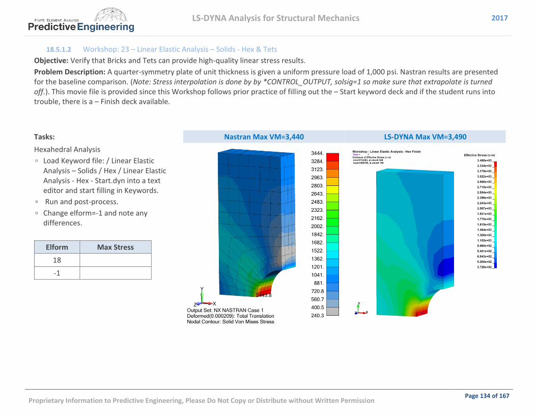
LS-DYNA Analysis for Structural Mechanics 2017
Proprietary Information to Predictive Engineering, Please Do Not Copy or Distribute without Written Permission Page 134 of 167
18.5.1.2 Workshop: 23 – Linear Elastic Analysis – Solids - Hex & Tets
Objective: Verify that Bricks and Tets can provide high-quality linear stress results.
Problem Description: A quarter-symmetry plate of unit thickness is given a uniform pressure load of 1,000 psi. Nastran results are presented for the baseline comparison. (Note: Stress interpolation is done by by *CONTROL_OUTPUT, solsig=1 so make sure that extrapolate is turned off.). This movie file is provided since this Workshop follows prior practice of filling out the – Start keyword deck and if the student runs into trouble, there is a – Finish deck available.
Tasks: Nastran Max VM=3,440 LS-DYNA Max VM=3,490
Hexahedral Analysis
▫ Load Keyword file: / Linear Elastic Analysis – Solids / Hex / Linear Elastic Analysis - Hex - Start.dyn into a text editor and start filling in Keywords.
▫ Run and post-process.
▫ Change elform=-1 and note any differences.
Elform Max Stress
18
-1
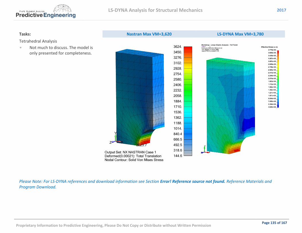
LS-DYNA Analysis for Structural Mechanics 2017
Proprietary Information to Predictive Engineering, Please Do Not Copy or Distribute without Written Permission Page 135 of 167
Tasks: Nastran Max VM=3,620 LS-DYNA Max VM=3,780
Tetrahedral Analysis
▫ Not much to discuss. The model is only presented for completeness.
Please Note: For LS-DYNA references and download information see Section Error! Reference source not found. Reference Materials and Program Download.

LS-DYNA Analysis for Structural Mechanics 2017
Proprietary Information to Predictive Engineering, Please Do Not Copy or Distribute without Written Permission Page 136 of 167
18.6 BEAM ELEMENT TECHNOLOGY FOR LINEAR ELASTIC STRESS ANALYSIS
LS-DYNA beam element formulations are quite diverse and provide broad modeling flexibility. When the term “resultant” is used for the ELFORM description, it signifies that only displacements and forces are calculated for the element. For explicit work, ELFORM=1 is the default while for implicit work ELFORM=4 is recommended. Although ELFORM=13 matches exactly with standard Nastran beam element formulation, it is a resultant formulation and stresses are not calculated and it is only applicable to linear behavior.
For all the standard LS-DYNA beam element formulations where stress is calculated, one needs to think about the type of quadrature rule (QR) is desired to recover stresses. It is identical to that for shell and solid elements but with a twist.
Beam Integration (QR) Setting
Beam integration is defined by the QR setting and can be one point or 2x2 Guass, 3x3 Guass, 3x3 Lobatto or 4x4 Guass as shown in the figure. Additionally, if necessary, one can also define specialized integration rules via *INTEGRATION_BEAM.
For beam elements, the integration is performed at one-point along the axis (mid-point of the beam) and then multiple points in-plane per QR=2, 3, 4 or 5.
The integration rule can be considered similar to that for shell elements based on the NIP setting to capture through thickness plasticity where for accuracy reasons NIP=5 is preferred.
For linear analysis, QR=4 is recommended and for plasticity analysis, QR=5 is a better choice.
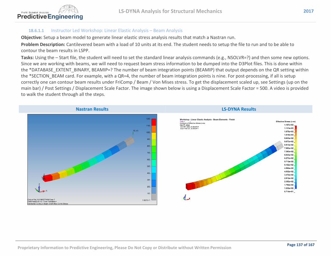
LS-DYNA Analysis for Structural Mechanics 2017
Proprietary Information to Predictive Engineering, Please Do Not Copy or Distribute without Written Permission Page 137 of 167
18.6.1.1 Instructor Led Workshop: Linear Elastic Analysis – Beam Analysis
Objective: Setup a beam model to generate linear elastic stress analysis results that match a Nastran run.
Problem Description: Cantilevered beam with a load of 10 units at its end. The student needs to setup the file to run and to be able to contour the beam results in LSPP.
Tasks: Using the – Start file, the student will need to set the standard linear analysis commands (e.g., NSOLVR=?) and then some new options. Since we are working with beams, we will need to request beam stress information to be dumped into the D3Plot files. This is done within the *DATABASE_EXTENT_BINARY, BEAMIP=? The number of beam integration points (BEAMIP) that output depends on the QR setting within the *SECTION_BEAM card. For example, with a QR=4, the number of beam integration points is nine. For post-processing, if all is setup correctly one can contour beam results under FriComp / Beam / Von Mises stress. To get the displacement scaled up, see Settings (up on the main bar) / Post Settings / Displacement Scale Factor. The image shown below is using a Displacement Scale Factor = 500. A video is provided to walk the student through all the steps.
Nastran Results LS-DYNA Results
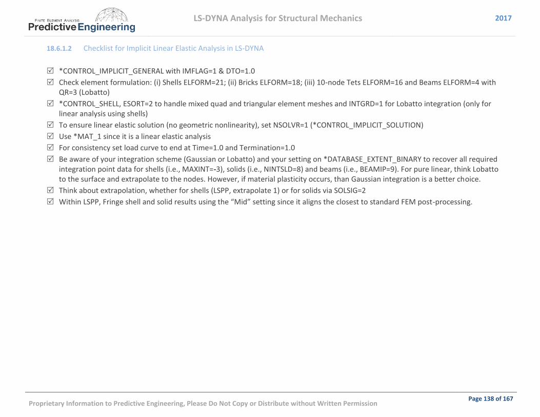
LS-DYNA Analysis for Structural Mechanics 2017
Proprietary Information to Predictive Engineering, Please Do Not Copy or Distribute without Written Permission Page 138 of 167
18.6.1.2 Checklist for Implicit Linear Elastic Analysis in LS-DYNA
*CONTROL_IMPLICIT_GENERAL with IMFLAG=1 & DTO=1.0
Check element formulation: (i) Shells ELFORM=21; (ii) Bricks ELFORM=18; (iii) 10-node Tets ELFORM=16 and Beams ELFORM=4 with QR=3 (Lobatto)
*CONTROL_SHELL, ESORT=2 to handle mixed quad and triangular element meshes and INTGRD=1 for Lobatto integration (only for linear analysis using shells)
To ensure linear elastic solution (no geometric nonlinearity), set NSOLVR=1 (*CONTROL_IMPLICIT_SOLUTION)
Use *MAT_1 since it is a linear elastic analysis
For consistency set load curve to end at Time=1.0 and Termination=1.0
Be aware of your integration scheme (Gaussian or Lobatto) and your setting on *DATABASE_EXTENT_BINARY to recover all required integration point data for shells (i.e., MAXINT=-3), solids (i.e., NINTSLD=8) and beams (i.e., BEAMIP=9). For pure linear, think Lobatto to the surface and extrapolate to the nodes. However, if material plasticity occurs, than Gaussian integration is a better choice.
Think about extrapolation, whether for shells (LSPP, extrapolate 1) or for solids via SOLSIG=2
Within LSPP, Fringe shell and solid results using the “Mid” setting since it aligns the closest to standard FEM post-processing.

LS-DYNA Analysis for Structural Mechanics 2017
Proprietary Information to Predictive Engineering, Please Do Not Copy or Distribute without Written Permission Page 139 of 167
18.7 GEOMETRIC AND MATERIAL NONLINEARITY
In this section we show how LS-DYNA implicit handles geometry and material nonlinearity. For the explicit solver, the solution of high nonlinearities is typically not an issue unless we are talking about massive element distortions or compaction of foams. We will treat this section in the classic sense and cover geometric nonlinearity as buckling and material nonlinearity as plasticity.
A nice engineering review of nonlinearity and how LS-DYNA can solve these problems using the implicit technique is found in the Class Reference Notes / Implicit Analysis / DYNAmore Implicit Users Guide /LS-DYNA Implicit Users Guide.pdf. If you have not read this article, one should review it while the Workshop exercise on buckling is solving (since it’ll take a few minutes).
To summarize what it means to do nonlinear analysis, the DYNAmore article provides a succinct list:
▫ non-linear material models (plasticity); ▫ contact; ▫ large deformations; ▫ non-linear constraints (such as joints); ▫ non-linear loading (such as follower forces, where the force direction is defined relative to the deformed geometry); ▫ stress stiffening (guitar string effect).
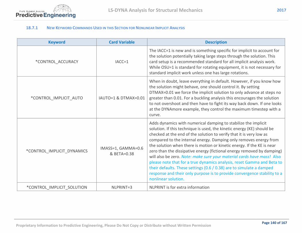
LS-DYNA Analysis for Structural Mechanics 2017
Proprietary Information to Predictive Engineering, Please Do Not Copy or Distribute without Written Permission Page 140 of 167
NEW KEYWORD COMMANDS USED IN THIS SECTION FOR NONLINEAR IMPLICIT ANALYSIS 18.7.1
Keyword Card Variable Description
*CONTROL_ACCURACY IACC=1
The IACC=1 is new and is something specific for implicit to account for the solution potentially taking large steps through the solution. This card setup is a recommended standard for all implicit analysis work. While OSU=1 is standard for rotating equipment, it is not necessary for standard implicit work unless one has large rotations.
*CONTROL_IMPLICIT_AUTO IAUTO=1 & DTMAX=0.01
When in doubt, leave everything in default. However, if you know how the solution might behave, one should control it. By setting DTMAX=0.01 we force the implicit solution to only advance at steps no greater than 0.01. For a buckling analysis this encourages the solution to not overshoot and then have to fight its way back down. If one looks at the DYNAmore example, they control the maximum timestep with a curve.
*CONTROL_IMPLICIT_DYNAMICS IMASS=1, GAMMA=0.6
& BETA=0.38
Adds dynamics with numerical damping to stabilize the implicit solution. If this technique is used, the kinetic energy (KE) should be checked at the end of the solution to verify that it is very low as compared to the internal energy. Damping only removes energy from the solution when there is motion or kinetic energy. If the KE is near zero than the dissipative energy (fictional energy removed by damping) will also be zero. Note: make sure your material cards have mass! Also please note that for a true dynamics analysis, reset Gamma and Beta to their defaults. These settings (0.6 / 0.38) are to simulate a damped response and their only purpose is to provide convergence stability to a nonlinear solution.
*CONTROL_IMPLICIT_SOLUTION NLPRINT=3 NLPRINT is for extra information

LS-DYNA Analysis for Structural Mechanics 2017
Proprietary Information to Predictive Engineering, Please Do Not Copy or Distribute without Written Permission Page 141 of 167
WORKSHOP: 24 – NONLINEAR BUCKLING OF BEER CAN 18.7.2
Introduction: The classic example is a slender column buckling and one can solve this problem with a simple hand calculation using Euler’s formula or solve it with a standard FEA technique. A review of basic FEA buckling using FEMAP and NX Nastran can be found in the Reading Assignments folder as: Predictive Engineering Buckling White Paper Rev-1. To keep things interesting, we’ll do a beer can and make the material out of aluminum using *MAT_098.
Objective: Setup model to solve one of the trickiest nonlinear geometric buckling problems in mechanics
Problem Description: The buckling of thin-walled cylinder is a very complex problem. We are going to make it even more difficult by using a force to drive the buckling and not a slowly increasing displacement load (although a companion model is given with a moving translational load). The cylinder is constrained on both ends and the force load is applied at the top over a load interval where buckling occurs prior to full load application.
Tasks: Prior to Buckling Post Buckled
▫ Open in a text editor Nonlinear Buckling of Beer Can – Start.dyn and inspect the Keywords.
▫ Enter data in the Keywords discussed within this section and then run the model.
▫ Review results and create XY cross-plot in LSPP showing Force (Y-axis) and Displacement (X-axis). The accompanying Movie file will show how to do a cross plot and also add a Timeline plot to the graphic.
Extra Credit: If you have time, rerun the model as a buckling analysis within LS-DYNA. This can be done by adding the *CONTROL_BUCKLE card and then changing the endtime to a time prior to buckling (we just want to load the can and not crush it). The buckling value (Freq = ) is the load scale factor that would cause buckling.

LS-DYNA Analysis for Structural Mechanics 2017
Proprietary Information to Predictive Engineering, Please Do Not Copy or Distribute without Written Permission Page 142 of 167
CHECKLIST FOR IMPLICIT NONLINEAR ANALYSIS IN LS-DYNA 18.7.3
*CONTROL_IMPLICIT_ACCURACY with IACC=1
*CONTROL_IMPLICIT_AUTO with IAUTO=1 and DTMAX=0.1 or use a “curve” to define solution keypoints
*CONTROL_IMPLICIT_DYNAMICS with IMASS=1, GAMMA=0.6 and BETA=0.38 for damped dynamics to assist in solution stability, e.g., when buckling occurs. Note: If a true transient dynamic analysis is required, then the values of GAMMA and BETA should be set to their defaults.
*CONTROL_IMPLICIT_GENERAL with IMFLAG=1 & DTO at 0.1 or some thoughtful initial timestep value
Check element formulation: (i) Shells ELFORM= -16 with NIP=5; (ii) Bricks ELFORM=-1; (iii) 10-node Tets ELFORM=16 and Beams ELFORM=4 with QR=4
*CONTROL_IMPLICIT_SOLUTION (all defaults) and NLPRINT=3 to print out convergence information to the screen
*CONTROL_OUTPUT with SOLSIG=2 for solid element extrapolation of integration point stresses to the nodes
If the analysis is not dynamics based, set load curve to end at Time=1.0 and Termination=1.0 for consistency
*DATABASE_EXTENT_BINARY to recover integration point data for shells, solids and beams via MAXINT=-3, BEAMIP=16 and NINTSLD=8.
In post-processing of stress data, fringe shell and solid results using the “Mid” setting since it aligns the closest to standard FEM post-processing
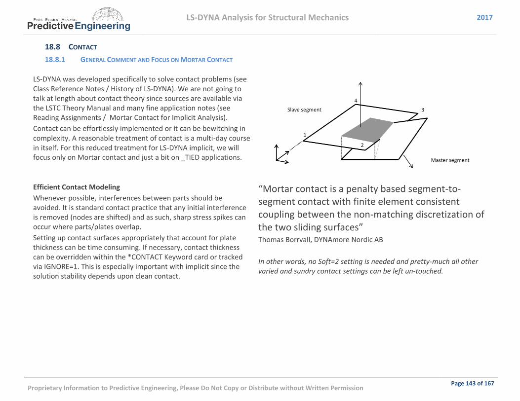
LS-DYNA Analysis for Structural Mechanics 2017
Proprietary Information to Predictive Engineering, Please Do Not Copy or Distribute without Written Permission Page 143 of 167
18.8 CONTACT
GENERAL COMMENT AND FOCUS ON MORTAR CONTACT 18.8.1
LS-DYNA was developed specifically to solve contact problems (see Class Reference Notes / History of LS-DYNA). We are not going to talk at length about contact theory since sources are available via the LSTC Theory Manual and many fine application notes (see Reading Assignments / Mortar Contact for Implicit Analysis).
Contact can be effortlessly implemented or it can be bewitching in complexity. A reasonable treatment of contact is a multi-day course in itself. For this reduced treatment for LS-DYNA implicit, we will focus only on Mortar contact and just a bit on _TIED applications.
Efficient Contact Modeling
Whenever possible, interferences between parts should be avoided. It is standard contact practice that any initial interference is removed (nodes are shifted) and as such, sharp stress spikes can occur where parts/plates overlap.
Setting up contact surfaces appropriately that account for plate thickness can be time consuming. If necessary, contact thickness can be overridden within the *CONTACT Keyword card or tracked via IGNORE=1. This is especially important with implicit since the solution stability depends upon clean contact.
“Mortar contact is a penalty based segment-to-segment contact with finite element consistent coupling between the non-matching discretization of the two sliding surfaces”
Thomas Borrvall, DYNAmore Nordic AB
In other words, no Soft=2 setting is needed and pretty-much all other varied and sundry contact settings can be left un-touched.

LS-DYNA Analysis for Structural Mechanics 2017
Proprietary Information to Predictive Engineering, Please Do Not Copy or Distribute without Written Permission Page 144 of 167
GENERAL MORTAR CONTACT TYPES 18.8.2
For general contact, the list is short and simple:
4. *CONTACT_AUTOMATIC_SINGLE_SURFACE_MORTAR
5. *CONTACT_AUTOMATIC_SURFACE_TO_SURFACE_MORTAR
How Mortar contact treats penetrations is a subject of some discussion since it is one known mechanism that can destroy convergence. From the Keyword Manual – Implicit Section (and now would be a good time to do some reading):
Most of these options are self-explanatory but IGNORE=4 provides the ability to handle initial interpenetrations. A dedicated workshop will cover this behavior since it is quite useful for interference fits.

LS-DYNA Analysis for Structural Mechanics 2017
Proprietary Information to Predictive Engineering, Please Do Not Copy or Distribute without Written Permission Page 145 of 167
18.8.2.1 Workshop: 25A – Implicit Contact – Basic Mechanics with Bolt Preload
Objective: Get familiar with contact and being able to check your model by investigating the contact forces generated between the two surfaces pulled together by a bolt preload and then by the “lever” load (Y-axis).
Model Description: A simple plate structure is bolted together with the bolts given a hefty bolt preload. Once this is done, a horizontal (Y-axis) load is applied that tilts the vertical plate over.
Acknowledgements: This example is courtesy from DYNAmore with some modifications.
Workshop Tasks
4. Load model Basic Mechanics with Bolt Preload – Start and setup mortar contact between the three parts using SURFACE_TO_SURFACE between parts 1 & 3 and then 1 & 2. Investigate how bolt preload is done via a section through part 3 (the bolts). Run note lack of convergence. Add IGNORE=1 to contact card.
5. Check for contact interference within LSPP (Application / Model Checking / General Checking / Contact Check. Check interference, make mental note and proceed to analyze model. Note excessive iterations (100+) on first effort.
6. Kill analysis and add IGNORE=1 or =2 via *CONTROL_CONTACT (Why do you think in this case they provide equivalent results?). Re-analyze.
7. Plot the resultant contact force between the L-Bracket (part 1) and the bottom plate (part 2). Note that the preload increases the contact force linearly up to the application of the horizontal “lever” load. (*DATABASE_RCFORC)
8. Create a Part Set with all three parts and then switch the contact to SINGLE_SURFACE and create a *CONTACT_FORCE_TRANSDUCER for the base part. Re-analyze and plot the force transducer result.
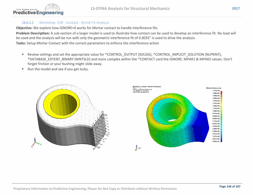
LS-DYNA Analysis for Structural Mechanics 2017
Proprietary Information to Predictive Engineering, Please Do Not Copy or Distribute without Written Permission Page 146 of 167
18.8.2.2 Workshop: 25B - Contact - Shrink Fit Analysis
Objective: We explore how IGNORE=4 works for Mortar contact to handle interference fits
Problem Description: A sub-section of a larger model is used to illustrate how contact can be used to develop an interference fit. No load will be used and the analysis will be run with only the geometric interference fit of 0.0035” is used to drive the analysis.
Tasks: Setup Mortar Contact with the correct parameters to enforce the interference action
Review settings and set the appropriate value for *CONTROL_OUTPUT (SOLSIG), *CONTROL_IMPLICIT_SOLUTION (NLPRINT), *DATABASE_EXTENT_BINARY (NINTSLD) and more complex within the *CONTACT card the IGNORE, MPAR1 & MPAR2 values. Don’t forget friction or your bushing might slide away.
Run the model and see if you get lucky.

LS-DYNA Analysis for Structural Mechanics 2017
Proprietary Information to Predictive Engineering, Please Do Not Copy or Distribute without Written Permission Page 147 of 167
TIED CONTACT FOR MESH TRANSITIONS, WELDING AND GLUING 18.8.3
Given the idealization difficulty of system modeling, the ability to tie together different mesh densities (e.g., hex-to-hex or tet-to-hex), snap together parts along a weld-line or just glue sections together (e.g., plate edge to a solid mesh) is an amazingly useful ability and implicit LS-DYNA provides a very complete Tied Contact tool box to work with.
The emphasis of this course to provide an overview of the basics to get started efficiently with LS-DYNA, a short list of recommended *KEYWORDS for implicit Tied Contact are presented.
It is also suggested that this would be good time to review the implicit section of the Keyword Manual under “tied”. Keep in mind that it is better to use fewer options but understand more completely what each command does. For example, the _SURFACE option tells LS-DYNA to only look at the surface of the MST that is provided within the Keyword Card. For example, if a Part is specified, it only looks at the surface of this Part as eligible for Tied Contact and nothing in its interior.
When a Solid Mesh is Used (Translational DOF Tied)
*CONTACT_TIED_NODES_TO_SURFACE (planer connection)
*CONTACT_TIED_NODES_TO_SURFACE_CONSTRAINED_OFFSET (When the mesh is offset)
When a Shell Mesh is Used or attaching beams to a shell mesh (All Six DOF Tied)
*CONTACT_TIED_SHELL_EDGE_TO_SURFACE
*CONTACT_TIED_SHELL_EDGE_TO_SURFACE_CONSTRAINED_OFFSET
General Comments
▫ _TIED (no _OFFSET) implies that the slave surface is co-planer or if it isn’t, it’ll move it to be adjacent to the Master surface. And, BTW, it’ll only move it if is “close” to the Master surface (Read The Manual (RTM)). One can override the default search distance by specifying a negative search distance on the SST MST fields. Please note that one has to specify both SST and MST with a negative number for the search distance. When in doubt – RTM.
▫ _OFFSET will not move your slave surface but you may need to expand your search distance to get things to tie together. This is where setting negative values on SST and MST come in handy. Be aware that on the _NODES side that if the distance is too large you can pick up interior notes if you specify the SST using a PART.
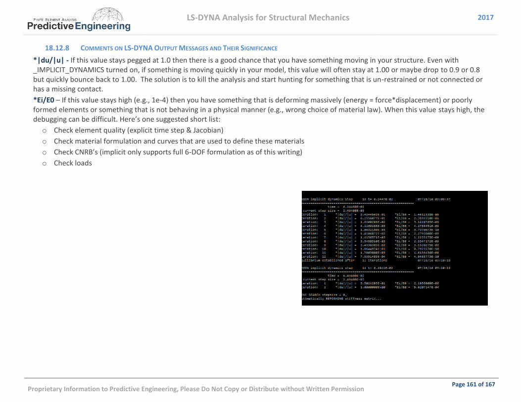
LS-DYNA Analysis for Structural Mechanics 2017
Proprietary Information to Predictive Engineering, Please Do Not Copy or Distribute without Written Permission Page 161 of 167
COMMENTS ON LS-DYNA OUTPUT MESSAGES AND THEIR SIGNIFICANCE 18.12.8
*|du/|u| - If this value stays pegged at 1.0 then there is a good chance that you have something moving in your structure. Even with _IMPLICIT_DYNAMICS turned on, if something is moving quickly in your model, this value will often stay at 1.00 or maybe drop to 0.9 or 0.8 but quickly bounce back to 1.00. The solution is to kill the analysis and start hunting for something that is un-restrained or not connected or has a missing contact.
*Ei/E0 – If this value stays high (e.g., 1e-4) then you have something that is deforming massively (energy = force*displacement) or poorly formed elements or something that is not behaving in a physical manner (e.g., wrong choice of material law). When this value stays high, the debugging can be difficult. Here’s one suggested short list:
o Check element quality (explicit time step & Jacobian)
o Check material formulation and curves that are used to define these materials
o Check CNRB’s (implicit only supports full 6-DOF formulation as of this writing)
o Check loads
LS-DYNA Analysis for Structural Mechanics 2017
Proprietary Information to Predictive Engineering, Please Do Not Copy or Distribute without Written Permission Page 162 of 167
19. DISCRETE ELEMENT METHOD
See Class Reference Notes / DEM / Predictive Engineering Discussion of LS-DYNA Meshfree Methods.pptx

LS-DYNA Analysis for Structural Mechanics 2017
Proprietary Information to Predictive Engineering, Please Do Not Copy or Distribute without Written Permission Page 163 of 167
20. FLUID STRUCTURE INTERACTION AND MULTI-PHYSICS IN LS-DYNA
See Class Reference Notes / Multi-Physics / LS-DYNA Multi-Physics.ppsx

LS-DYNA Analysis for Structural Mechanics 2017
Proprietary Information to Predictive Engineering, Please Do Not Copy or Distribute without Written Permission Page 167 of 167

LS-DYNA Analysis for Structural Mechanics 2017
Proprietary Information to Predictive Engineering, Please Do Not Copy or Distribute without Written Permission Page 168 of 167