ls-svmlab toolbox user’s guide - search...

LS-SVMlab Toolbox User’s Guideversion 1.5

K. Pelckmans, J.A.K. Suykens, T. Van Gestel, J. De Brabanter,L. Lukas, B. Hamers, B. De Moor, J. Vandewalle

Katholieke Universiteit Leuven

Department of Electrical Engineering, ESAT-SCD-SISTA

Kasteelpark Arenberg 10, B-3001 Leuven-Heverlee, Belgium

{ kristiaan.pelckmans, johan.suykens }@esat.kuleuven.ac.be

http://www.esat.kuleuven.ac.be/sista/lssvmlab/

ESAT-SCD-SISTA Technical Report 02-145

February 2003

Acknowledgements

Research supported by Research Council K.U.Leuven: GOA-Mefisto 666, IDO (IOTAoncology, genetic networks), several PhD/postdoc & fellow grants; Flemish Govern-ment: FWO: PhD/postdoc grants, G.0407.02 (support vector machines), projectsG.0115.01 (microarrays/oncology), G.0240.99 (multilinear algebra), G.0080.01 (col-lective intelligence), G.0413.03 (inference in bioi), G.0388.03 (microarrays for clinicaluse), G.0229.03 (ontologies in bioi), G.0197.02 (power islands), G.0141.03 (identifi-cation and cryptography), G.0491.03 (control for intensive care glycemia), G.0120.03(QIT), research communities (ICCoS, ANMMM); AWI: Bil. Int. Collaboration Hun-gary, Poland, South Africa; IWT: PhD Grants, STWW-Genprom (gene promotorprediction), GBOU-McKnow (knowledge management algorithms), GBOU-SQUAD(quorum sensing), GBOU-ANA (biosensors); Soft4s (softsensors) Belgian Federal Gov-ernment: DWTC (IUAP IV-02 (1996-2001) and IUAP V-22 (2002-2006)); PODO-II(CP/40: TMS and sustainibility); EU: CAGE; ERNSI; Eureka 2063-IMPACT; Eureka2419-FliTE; Contract Research/agreements: Data4s, Electrabel, Elia, LMS, IPCOS,VIB; JS is a professor at K.U.Leuven Belgium and a postdoctoral researcher with FWOFlanders. TVG is postdoctoral researcher with FWO Flanders. BDM and JWDW arefull professors at K.U.Leuven Belgium.

1

Contents

1 Introduction 4

2 A birds eye view on LS-SVMlab 52.1 Classification and Regression . . . . . . . . . . . . . . . . . . . . . . . . . . . . . . 5

2.1.1 Classification Extensions . . . . . . . . . . . . . . . . . . . . . . . . . . . . . 62.1.2 Tuning, Sparseness, Robustness . . . . . . . . . . . . . . . . . . . . . . . . . 62.1.3 Bayesian Framework . . . . . . . . . . . . . . . . . . . . . . . . . . . . . . . 8

2.2 NARX Models and Prediction . . . . . . . . . . . . . . . . . . . . . . . . . . . . . . 82.3 Unsupervised Learning . . . . . . . . . . . . . . . . . . . . . . . . . . . . . . . . . . 82.4 Solving Large Scale Problems with Fixed Size LS-SVM . . . . . . . . . . . . . . . . 9

3 LS-SVMlab toolbox examples 103.1 Classification . . . . . . . . . . . . . . . . . . . . . . . . . . . . . . . . . . . . . . . 10

3.1.1 Hello world... . . . . . . . . . . . . . . . . . . . . . . . . . . . . . . . . . . . 103.1.2 The Ripley data set . . . . . . . . . . . . . . . . . . . . . . . . . . . . . . . 123.1.3 Bayesian Inference for Classification . . . . . . . . . . . . . . . . . . . . . . 143.1.4 Multi-class coding . . . . . . . . . . . . . . . . . . . . . . . . . . . . . . . . 16

3.2 Regression . . . . . . . . . . . . . . . . . . . . . . . . . . . . . . . . . . . . . . . . . 173.2.1 A Simple Sinc Example . . . . . . . . . . . . . . . . . . . . . . . . . . . . . 173.2.2 Bayesian Inference for Regression . . . . . . . . . . . . . . . . . . . . . . . . 193.2.3 Using the object oriented model interface . . . . . . . . . . . . . . . . . . . 203.2.4 Robust Regression . . . . . . . . . . . . . . . . . . . . . . . . . . . . . . . . 223.2.5 Multiple Output Regression . . . . . . . . . . . . . . . . . . . . . . . . . . . 233.2.6 A Time-Series Example: Santa Fe Laser Data Prediction . . . . . . . . . . 243.2.7 Fixed size LS-SVM . . . . . . . . . . . . . . . . . . . . . . . . . . . . . . . . 25

3.3 Unsupervised Learning using kernel based Principal Component Analysis . . . . . 28

A MATLAB functions 29A.1 General Notation . . . . . . . . . . . . . . . . . . . . . . . . . . . . . . . . . . . . . 29A.2 Index of Function Calls . . . . . . . . . . . . . . . . . . . . . . . . . . . . . . . . . 30

A.2.1 Training and Simulation . . . . . . . . . . . . . . . . . . . . . . . . . . . . . 30A.2.2 Object Oriented Interface . . . . . . . . . . . . . . . . . . . . . . . . . . . . 31A.2.3 Training and Simulating Functions . . . . . . . . . . . . . . . . . . . . . . . 32A.2.4 Kernel Functions . . . . . . . . . . . . . . . . . . . . . . . . . . . . . . . . . 33A.2.5 Tuning, Sparseness and Robustness . . . . . . . . . . . . . . . . . . . . . . . 34A.2.6 Classification Extensions . . . . . . . . . . . . . . . . . . . . . . . . . . . . . 35A.2.7 Bayesian Framework . . . . . . . . . . . . . . . . . . . . . . . . . . . . . . . 36A.2.8 NARX models and Prediction . . . . . . . . . . . . . . . . . . . . . . . . . . 37A.2.9 Unsupervised learning . . . . . . . . . . . . . . . . . . . . . . . . . . . . . . 38A.2.10 Fixed Size LS-SVM . . . . . . . . . . . . . . . . . . . . . . . . . . . . . . . 39A.2.11 Demos . . . . . . . . . . . . . . . . . . . . . . . . . . . . . . . . . . . . . . . 40

A.3 Alphabetical List of Function Calls . . . . . . . . . . . . . . . . . . . . . . . . . . . 41

2

A.3.1 AFE . . . . . . . . . . . . . . . . . . . . . . . . . . . . . . . . . . . . . . . . 41A.3.2 bay errorbar . . . . . . . . . . . . . . . . . . . . . . . . . . . . . . . . . . . 42A.3.3 bay initlssvm . . . . . . . . . . . . . . . . . . . . . . . . . . . . . . . . . . 44A.3.4 bay lssvm . . . . . . . . . . . . . . . . . . . . . . . . . . . . . . . . . . . . . 45A.3.5 bay lssvmARD . . . . . . . . . . . . . . . . . . . . . . . . . . . . . . . . . . . 47A.3.6 bay modoutClass . . . . . . . . . . . . . . . . . . . . . . . . . . . . . . . . . 49A.3.7 bay optimize . . . . . . . . . . . . . . . . . . . . . . . . . . . . . . . . . . . 51A.3.8 bay rr . . . . . . . . . . . . . . . . . . . . . . . . . . . . . . . . . . . . . . . 53A.3.9 code, codelssvm . . . . . . . . . . . . . . . . . . . . . . . . . . . . . . . . 55A.3.10 crossvalidate . . . . . . . . . . . . . . . . . . . . . . . . . . . . . . . . . . 58A.3.11 deltablssvm . . . . . . . . . . . . . . . . . . . . . . . . . . . . . . . . . . . 61A.3.12 denoise kpca . . . . . . . . . . . . . . . . . . . . . . . . . . . . . . . . . . . 62A.3.13 eign . . . . . . . . . . . . . . . . . . . . . . . . . . . . . . . . . . . . . . . . 64A.3.14 initlssvm, changelssvm . . . . . . . . . . . . . . . . . . . . . . . . . . . . 65A.3.15 kentropy . . . . . . . . . . . . . . . . . . . . . . . . . . . . . . . . . . . . . 68A.3.16 kernel matrix . . . . . . . . . . . . . . . . . . . . . . . . . . . . . . . . . . 69A.3.17 kpca . . . . . . . . . . . . . . . . . . . . . . . . . . . . . . . . . . . . . . . . 70A.3.18 latentlssvm . . . . . . . . . . . . . . . . . . . . . . . . . . . . . . . . . . . 71A.3.19 leaveoneout . . . . . . . . . . . . . . . . . . . . . . . . . . . . . . . . . . . 73A.3.20 leaveoneout lssvm . . . . . . . . . . . . . . . . . . . . . . . . . . . . . . . 75A.3.21 lin kernel, MLP kernel, poly kernel, RBF kernel . . . . . . . . . . . . 77A.3.22 linf, mae, medae, misclass, mse, trimmedmse . . . . . . . . . . . . . 78A.3.23 plotlssvm . . . . . . . . . . . . . . . . . . . . . . . . . . . . . . . . . . . . 80A.3.24 predict . . . . . . . . . . . . . . . . . . . . . . . . . . . . . . . . . . . . . . 82A.3.25 prelssvm, postlssvm . . . . . . . . . . . . . . . . . . . . . . . . . . . . . . 84A.3.26 rcrossvalidate . . . . . . . . . . . . . . . . . . . . . . . . . . . . . . . . . 85A.3.27 ridgeregress . . . . . . . . . . . . . . . . . . . . . . . . . . . . . . . . . . 87A.3.28 robustlssvm . . . . . . . . . . . . . . . . . . . . . . . . . . . . . . . . . . . 88A.3.29 roc . . . . . . . . . . . . . . . . . . . . . . . . . . . . . . . . . . . . . . . . 89A.3.30 simlssvm . . . . . . . . . . . . . . . . . . . . . . . . . . . . . . . . . . . . . 91A.3.31 sparselssvm . . . . . . . . . . . . . . . . . . . . . . . . . . . . . . . . . . . 93A.3.32 trainlssvm . . . . . . . . . . . . . . . . . . . . . . . . . . . . . . . . . . . . 94A.3.33 tunelssvm, linesearch & gridsearch . . . . . . . . . . . . . . . . . . . . 96A.3.34 validate . . . . . . . . . . . . . . . . . . . . . . . . . . . . . . . . . . . . . 100A.3.35 windowize & windowizeNARX . . . . . . . . . . . . . . . . . . . . . . . . . . 102

3

Chapter 1

Introduction

Support Vector Machines (SVM) is a powerful methodology for solving problems in nonlinearclassification, function estimation and density estimation which has also led to many other recentdevelopments in kernel based learning methods in general [3, 16, 17, 34, 33]. SVMs have been in-troduced within the context of statistical learning theory and structural risk minimization. In themethods one solves convex optimization problems, typically quadratic programs. Least SquaresSupport Vector Machines (LS-SVM) are reformulations to standard SVMs [21, 28] which leadto solving linear KKT systems. LS-SVMs are closely related to regularization networks [5] andGaussian processes [37] but additionally emphasize and exploit primal-dual interpretations. Linksbetween kernel versions of classical pattern recognition algorithms such as kernel Fisher discrim-inant analysis and extensions to unsupervised learning, recurrent networks and control [22] areavailable. Robustness, sparseness and weightings [23] can be imposed to LS-SVMs where neededand a Bayesian framework with three levels of inference has been developed [29, 32]. LS-SVMalike primal-dual formulations are given to kernel PCA [24], kernel CCA and kernel PLS [25]. Forultra large scale problems and on-line learning a method of Fixed Size LS-SVM is proposed, whichis related to a Nystrom sampling [6, 35] with active selection of support vectors and estimation inthe primal space.

The present LS-SVMlab toolbox User’s Guide contains Matlab/C implementations for a num-ber of LS-SVM algorithms related to classification, regression, time-series prediction and unsuper-vised learning. References to commands in the toolbox are written in typewriter font.

A main reference and overview on least squares support vector machines is

J.A.K. Suykens, T. Van Gestel, J. De Brabanter, B. De Moor, J. Vandewalle,Least Squares Support Vector Machines,World Scientific, Singapore, 2002 (ISBN 981-238-151-1).

The LS-SVMlab homepage is

http://www.esat.kuleuven.ac.be/sista/lssvmlab/

The LS-SVMlab toolbox is made available under the GNU general license policy:

Copyright (C) 2002 KULeuven-ESAT-SCD

This program is free software; you can redistribute it and/or modify it under the termsof the GNU General Public License as published by the Free Software Foundation;either version 2 of the License, or (at your option) any later version.

This program is distributed in the hope that it will be useful, but WITHOUT ANYWARRANTY; without even the implied warranty of MERCHANTABILITY or FIT-NESS FOR A PARTICULAR PURPOSE. See the website of LS-SVMlab or the GNUGeneral Public License for a copy of the GNU General Public License specifications.

4

Chapter 2

A birds eye view on LS-SVMlab

The toolbox is mainly intended for use with the commercial Matlab package. However, the corefunctionality is written in C-code. The Matlab toolbox is compiled and tested for different com-puter architectures including Linux and Windows. Most functions can handle datasets up to 20000data points or more. LS-SVMlab’s interface for Matlab consists of a basic version for beginners aswell as a more advanced version with programs for multi-class encoding techniques and a Bayesianframework. Future versions will gradually incorporate new results and additional functionalities.

The organization of the toolbox is schematically shown in Figure 2.1. A number of functionsare restricted to LS-SVMs (these include the extension “lssvm” in the function name), the othersare generally usable. A number of demos illustrate how to use the different features of the toolbox.The Matlab function interfaces are organized in two principal ways: the functions can be calledeither in a functional way or using an object oriented structure (referred to as the model) as e.g. inNetlab [14], depending on the user’s choice1.

2.1 Classification and Regression

Function calls: trainlssvm, simlssvm, plotlssvm, prelssvm, postlssvm;Demos: Subsections 3.1, 3.2, demofun, democlass.

The Matlab toolbox is built around a fast LS-SVM training and simulation algorithm. Thecorresponding function calls can be used for classification as well as for function estimation. Thefunction plotlssvm displays the simulation results of the model in the region of the trainingpoints.

To avoid failures and ensure performance of the implementation, three different implementa-tions are included. The most performant is the CMEX implementation (lssvm.mex*), based onC-code linked with Matlab via the CMEX interface. More reliable (less system specific) is theC-compiled executable (lssvm.x) which passes the parameters to/from Matlab via a buffer file.Both use the fast conjugate gradient algorithm to solve the set of linear equations [8]. The C-codefor training takes advantage of previously calculated solutions by caching the firstly calculatedkernel evaluations up to 64 Mb of data. Less performant but stable, flexible and straightforwardcoded is the implementation in Matlab (lssvmMATLAB.m) which is based on the Matlab matrixdivision (backslash command \).

Functions for single and multiple output regression and classification are available. Trainingand simulation can be done for each output separately by passing different kernel functions, kerneland/or regularization parameters as a column vector. It is straightforward to implement otherkernel functions in the toolbox.

1See http://www.kernel-machines.org/software.html for other software in kernel based learning techniques.

5

model tuning

Fixed Size LS−SVM

AFE

kentropy

ridgeregress

bay_rr

NAR(X) & prediction

model validation

preprocessing

Basic

LS−SVMlab Toolbox Matlab/C

Bayesian framework

Advanced

windowize

predict

windowizeNARX

encoding

code_ECOC

code

prelssvm

postlssvm

tunelssvm

prunelssvm

weightedlssvm

crossvalidate

leaveoneout

validate

kpca

bay_lssvm

bay_optimize

lssvm MATLAB

simlssv

m

trainlssv

m

C−code

lssvm.mex*lssvm.xp

lotlssv

m

demos

Figure 2.1: Schematic illustration of the organization of LS-SVMlab. Each box contains the namesof the corresponding algorithms. The function names with extension “lssvm” are LS-SVM methodspecific. The dashed box includes all functions of a more advanced toolbox, the large grey boxthose that are included in the basic version.

The performance of a model depends on the scaling of the input and output data. An appro-priate algorithm detects and appropriately rescales continuous, categorical and binary variables(prelssvm, postlssvm).

2.1.1 Classification Extensions

Function calls: codelssvm, code, deltablssvm, roc, latentlssvm;Demos: Subsection 3.1, democlass.

A number of additional function files are available for the classification task. The latent vari-able of simulating a model for classification (latentlssvm) is the continuous result obtained bysimulation which is discretised for making the final decisions. The Receiver Operating Character-istic curve [9] (roc) can be used to measure the performance of a classifier. Multiclass classificationproblems are decomposed into multiple binary classification tasks [30]. Several coding schemes canbe used at this point: minimum output, one-versus-one, one-versus-all and error correcting codingschemes. To decode a given result, the Hamming distance, loss function distance and Bayesiandecoding can be applied. A correction of the bias term can be done, which is especially interestingfor small data sets.

2.1.2 Tuning, Sparseness, Robustness

Function calls: tunelssvm, validate, crossvalidate, leaveoneout, robustlssvm,

sparselssvm;Demos: Subsections 3.1.2, 3.1.4, 3.2.4, 3.2.6, demofun, democlass, demomodel.

A number of methods to estimate the generalization performance of the trained model areincluded. The estimate of the performance based on a fixed testset is calculated by validate. For

6

0 5000 10000 1500010

−2

10−1

100

101

102

103

compare implementation training implementations LS−SVMlab

size dataset

com

puta

tion

time

[in s

econ

ds]

Figure 2.2: Indication of the performance for the different training implementations of LS-SVMlab.The solid line indicates the performance of the CMEX interface. The dashed line shows theperformance of the CFILE interface and the dashed-dotted line indicated the performance of thepure MATLAB implementation.

7

classification, the rate of misclassifications (misclass) can be used. Estimates based on repeatedtraining and validation are given by crossvalidate and leaveoneout. The implementation ofthese include a bias correction term. A robust crossvalidation score function [4] is called byrcrossvalidate. These performance measures can be used to tune the hyper-parameters (e.g.the regularization and kernel parameters) of the LS-SVM (tunelssvm). Reducing the modelcomplexity of a LS-SVM can be done by iteratively pruning the less important support values(sparselssvm) [23]. In the case of outliers in the data or non-Gaussian noise, corrections to thesupport values will improve the model (robustlssvm) [23].

2.1.3 Bayesian Framework

Function calls: bay lssvm, bay optimize, bay lssvmARD, bay errorbar, bay modoutClass,

kpca, eign;Demos: Subsections 3.1.3, 3.2.2.

Functions for calculating the posterior probability of the model and hyper-parameters at dif-ferent levels of inference are available (bay_lssvm) [26, 32]. Errors bars are obtained by tak-ing into account model- and hyper-parameter uncertainties (bay_errorbar). For classification[29], one can estimate the posterior class probabilities (this is also called the moderated output)(bay_modoutClass). The Bayesian framework makes use of the eigenvalue decomposition of thekernel matrix. The size of the matrix grows with the number of data points. Hence, one needsapproximation techniques to handle large datasets. It is known that mainly the principal eigenval-ues and corresponding eigenvectors are relevant. Therefore, iterative approximation methods suchas the Nystrom method [31, 35] are included, which is also frequently used in Gaussian processes.Input selection can be done by Automatic Relevance Determination (bay_lssvmARD) [27]. In abackward variable selection, the third level of inference of the Bayesian framework is used to inferthe most relevant inputs of the problem.

2.2 NARX Models and Prediction

Function calls: predict, windowize;Demo: Subsection 3.2.6.

Extensions towards nonlinear NARX systems for time series applications are available [25].A NARX model can be built based on a nonlinear regressor by estimating in each iterationthe next output value given the past output (and input) measurements. A dataset is convertedinto a new input (the past measurements) and output set (the future output) by windowize andwindowizeNARX for respectively the time series case and in general the NARX case with exogenousinput. Iteratively predicting (in recurrent mode) the next output based on the previous predictionsand starting values is done by predict.

2.3 Unsupervised Learning

Function calls: kpca, denoise kpca;Demo: Subsection 3.3.

Unsupervised learning can be done by kernel based PCA (kpca) as described by [19], for whichrecently a primal-dual interpretation with support vector machine formulation has been given in[24], which has also be further extended to kernel canonical correlation analysis [25] and kernelPLS.

8

X

YTraining data set

Fixed sizeselected subset

Criterion

ϕ(.)

Regression in primal space

Figure 2.3: Fixed Size LS-SVM is a method for solving large scale regression and classificationproblems. The number of support vectors is pre-fixed beforehand and the support vectors areselected from a pool of training data. After estimating eigenfunctions in relation to a Nystromsampling with selection of the support vectors according to an entropy criterion, the LS-SVMmodel is estimated in the primal space.

2.4 Solving Large Scale Problems with Fixed Size LS-SVM

Function calls: demo fixedsize, AFE, kentropy;Demos: Subsection 3.2.7, demo fixedsize, demo fixedclass.

Classical kernel based algorithms like e.g. LS-SVM [21] typically have memory and compu-tational requirements of O(N2). Recently, work on large scale methods proposes solutions tocircumvent this bottleneck [25, 19].

For large datasets it would be advantageous to solve the least squares problem in the primalweight space because then the size of the vector of unknowns is proportional to the feature vectordimension and not to the number of datapoints. However, the feature space mapping inducedby the kernel is needed in order to obtain non-linearity. For this purpose, a method of fixed sizeLS-SVM is proposed [25] (Figure 2.3). Firstly the Nystrom method [29, 35] can be used to esti-mate the feature space mapping. The link between Nystrom sampling, kernel PCA and densityestimation has been discussed in [6]. In fixed size LS-SVM these links are employed together withthe explicit primal-dual LS-SVM interpretations. The support vectors are selected according toa quadratic Renyi entropy criterion (kentropy). In a last step a regression is done in the primalspace which makes the method suitable for solving large scale nonlinear function estimation andclassification problems. A Bayesian framework for ridge regression [11, 29] (bay_rr) can be usedto find a good regularization parameter. The method of fixed size LS-SVM is suitable for handlingvery large data sets, adaptive signal processing and transductive inference.

An alternative criterion for subset selection was presented by [1, 2], which is closely related to[35] and [19]. It measures the quality of approximation of the feature space and the space inducedby the subset (see Automatic Feature Extraction or AFE). In [35] the subset was taken as a randomsubsample from the data (subsample).

9

Chapter 3

LS-SVMlab toolbox examples

3.1 Classification

At first, the possibilities of the toolbox for classification tasks are illustrated.

3.1.1 Hello world...

A simple example shows how to start using the toolbox for a classification task. We start withconstructing a simple example dataset according to the correct formatting. Data are representedas matrices where each row of the matrix contains one datapoint:

>> X = 2.*rand(30,2)-1;

>> Y = sign(sin(X(:,1))+X(:,2));

>> X

X =

0.9003 -0.9695

-0.5377 0.4936

0.2137 -0.1098

-0.0280 0.8636

0.7826 -0.0680

0.5242 -0.1627

.... ....

-0.4556 0.7073

-0.6024 0.1871

>> Y

Y =

-1

-1

1

1

1

1

...

1

-1

10

−1 −0.8 −0.6 −0.4 −0.2 0 0.2 0.4 0.6 0.8 1

−1

−0.8

−0.6

−0.4

−0.2

0

0.2

0.4

0.6

0.8

1

X1

X2

LS−SVMγ=10,σ2=0.2

RBF , with 2 different classes;

class 1class 2

Figure 3.1: Figure generated by plotlssvm in the simple classification task.

In order to make an LS-SVM model, we need two extra parameters: γ (gam) is the regularizationparameter, determining the trade-off between the fitting error minimization and smoothness. Inthe common case of the RBF kernel, σ2 (sig2) is the bandwidth:

>> gam = 10;

>> sig2 = 0.2;

>> type = ’classification’;

>> [alpha,b] = trainlssvm({X,Y,type,gam,sig2,’RBF_kernel’});

The parameters and the variables relevant for the LS-SVM are passed as one cell. This cellallows for consistent default handling of LS-SVM parameters and syntactical grouping of relatedarguments. This definition should be used consistently throughout the use of that LS-SVM model.The corresponding object oriented interface to LS-SVMlab leads to shorter function calls (seedemomodel).

By default, the data are preprocessed by application of the function prelssvm to the rawdata and the function postlssvm on the predictions of the model. This option can explicitly beswitched off in the call:

>> [alpha,b] = trainlssvm({X,Y,type,gam,sig2,’RBF_kernel’,’original’});

or be switched on (by default):

>> [alpha,b] = trainlssvm({X,Y,type,gam,sig2,’RBF_kernel’,’preprocess’});

Remember to consistently use the same option in all successive calls.To evaluate new points for this model, the function simlssvm is used.

>> Xt = 2.*rand(10,2)-1;

>> Ytest = simlssvm({X,Y,type,gam,sig2,’RBF_kernel’},{alpha,b},Xt);

The LS-SVM result can be displayed if the dimension of the input data is 2.

>> plotlssvm({X,Y,type,gam,sig2,’RBF_kernel’},{alpha,b});

All plotting is done with this simple command. It looks for the best way of displaying the result(Figure 3.1).

11

3.1.2 The Ripley data set

The well-known Ripley dataset problem consists of two classes where the data for each class havebeen generated by a mixture of two Gaussian distributions (Figure 3.2a).

First, let us build an LS-SVM on the dataset and determine suitable hyperparameters:

>> % load dataset ...

>> type = ’classification’;

>> L_fold = 10; % L-fold crossvalidation

>> [gam,sig2] = tunelssvm({X,Y,type,1,1,’RBF_kernel’},[],...

’gridsearch’,{},’crossvalidate’,{X,Y,L_fold,’misclass’});


>> plotlssvm({X,Y,type,gam,sig2,’RBF_kernel’},{alpha,b});

The Receiver Operating Characteristic (ROC) curve gives information about the quality of theclassifier:


>> Y_latent = latentlssvm({X,Y,type,gam,sig2,’RBF_kernel’},{alpha,b},X);

>> [area,se,thresholds,oneMinusSpec,Sens]=roc(Y_latent,Y);

>> [thresholds oneMinusSpec Sens]

ans =

-2.1915 1.0000 1.0000

-1.1915 0.9920 1.0000

-1.1268 0.9840 1.0000

-1.0823 0.9760 1.0000

... ... ...

-0.2699 0.1840 0.9360

-0.2554 0.1760 0.9360

-0.2277 0.1760 0.9280

-0.1811 0.1680 0.9280

... ... ...

1.1184 0 0.0080

1.1220 0 0

2.1220 0 0

The corresponding ROC curve is shown on Figure 3.2c. This information can be used to furtherintroduce prior knowledge in the classifier. A bias term correction can be found from the previousoutcome:

>> plotlssvm({X,Y,type,gam,sig2,’RBF_kernel’},{alpha,-0.2277});

The result is shown in Figure 3.2d.

12

−1.2 −1 −0.8 −0.6 −0.4 −0.2 0 0.2 0.4 0.6 0.8−0.2

0

0.2

0.4

0.6

0.8

1

X1

X2

LS−SVMγ=10,σ2=1

RBF , with 2 different classes

class 1class 2

(a) Original Classifier

−1.2 −1 −0.8 −0.6 −0.4 −0.2 0 0.2 0.4 0.6 0.8−0.2

0

0.2

0.4

0.6

0.8

1

Probability of occurence of class 1

X1

X2

class 1class 2

(b) Moderated Output

0 0.1 0.2 0.3 0.4 0.5 0.6 0.7 0.8 0.9 10

0.1

0.2

0.3

0.4

0.5

0.6

0.7

0.8

0.9

1Receiver Operating Characteristic curve, area=0.96646, std = 0.011698

1 − Specificity

Sen

sitiv

ity

(c) ROC Curve

−1.2 −1 −0.8 −0.6 −0.4 −0.2 0 0.2 0.4 0.6 0.8−0.2

0

0.2

0.4

0.6

0.8

1

X1

X2

LS−SVMγ=10,σ2=1


class 1class 2

(d) Bias Term Correction

Figure 3.2: ROC curve and bias term correction on the Ripley classification task. (a) Original LS-SVM classifier. (b) Moderated output of the LS-SVM classifier on the Ripley data set. Shown arethe probabilities to belong to the positive class (magenta: probability towards 0, cyan: probabilitytowards 1). (c) Receiver Operating Characteristic curve. (d) The bias term correction can beused to avoid misclassifications for one of the two classes.

13

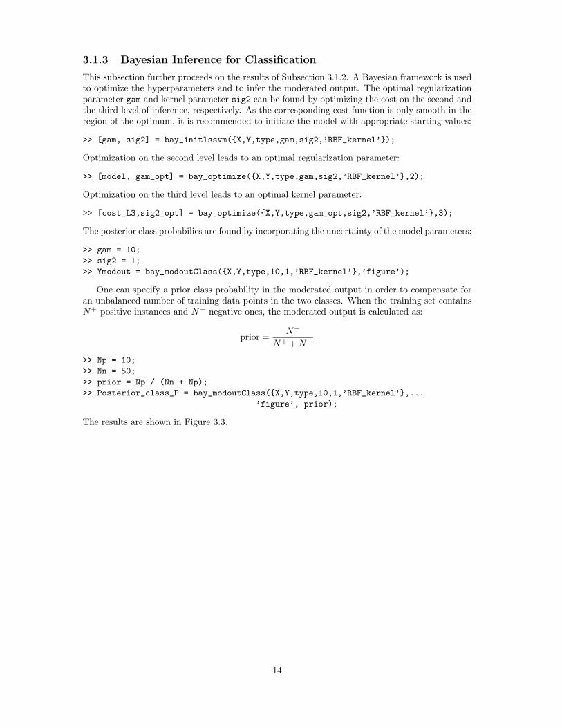
3.1.3 Bayesian Inference for Classification

This subsection further proceeds on the results of Subsection 3.1.2. A Bayesian framework is usedto optimize the hyperparameters and to infer the moderated output. The optimal regularizationparameter gam and kernel parameter sig2 can be found by optimizing the cost on the second andthe third level of inference, respectively. As the corresponding cost function is only smooth in theregion of the optimum, it is recommended to initiate the model with appropriate starting values:

>> [gam, sig2] = bay_initlssvm({X,Y,type,gam,sig2,’RBF_kernel’});

Optimization on the second level leads to an optimal regularization parameter:

>> [model, gam_opt] = bay_optimize({X,Y,type,gam,sig2,’RBF_kernel’},2);

Optimization on the third level leads to an optimal kernel parameter:

>> [cost_L3,sig2_opt] = bay_optimize({X,Y,type,gam_opt,sig2,’RBF_kernel’},3);

The posterior class probabilies are found by incorporating the uncertainty of the model parameters:

>> gam = 10;

>> sig2 = 1;

>> Ymodout = bay_modoutClass({X,Y,type,10,1,’RBF_kernel’},’figure’);

One can specify a prior class probability in the moderated output in order to compensate foran unbalanced number of training data points in the two classes. When the training set containsN+ positive instances and N− negative ones, the moderated output is calculated as:

prior =N+

N+ + N−

>> Np = 10;

>> Nn = 50;

>> prior = Np / (Nn + Np);

>> Posterior_class_P = bay_modoutClass({X,Y,type,10,1,’RBF_kernel’},...

’figure’, prior);

The results are shown in Figure 3.3.

14

−1.2 −1 −0.8 −0.6 −0.4 −0.2 0 0.2 0.4 0.6 0.8−0.2

0

0.2

0.4

0.6

0.8

1


X1

X2

class 1class 2

(a) Moderated Output

−1.2 −1 −0.8 −0.6 −0.4 −0.2 0 0.2 0.4 0.6 0.8−0.2

0

0.2

0.4

0.6

0.8

1


X1

X2

class 1class 2

(b) Unbalanced subset

−1.2 −1 −0.8 −0.6 −0.4 −0.2 0 0.2 0.4 0.6 0.8−0.2

0

0.2

0.4

0.6

0.8

1


X1

X2

class 1class 2

(c) With correction for unbalancing

Figure 3.3: (a) Moderated output of the LS-SVM classifier on the Ripley data set. The colorsindicate the probability to belong to a certain class; (b) This example shows the moderated outputof an unbalanced subset of the Ripley data; (c) One can compensate for unbalanced data in thecalculation of the moderated output. One can notice that the area of the green zone with thepositive samples increases by the compensation. The red zone shrinks accordingly.

15

−4 −3 −2 −1 0 1 2−3

−2

−1

0

1

2

3

X1

X2

1

2

2

2

2

112

class 1class 2class 3

Figure 3.4: LS-SVM multi-class example with one versus one encoding.

3.1.4 Multi-class coding

The following example shows how to use an encoding scheme for multi-class problems. Theencoding and decoding are seen as a separate and independent preprocessing and postprocessingstep respectively (Figure 3.5).

>> % load multiclass data ...

>> [Ycode, codebook, old_codebook] = code(Y,’code_MOC’);

>>

>> [alpha,b] = trainlssvm({X,Ycode,’classifier’,gam,sig2});

>> Yhc = simlssvm({X,Ycode,’classifier’,gam,sig2},{alpha,b},Xtest);

>>

>> Yhc = code(Yh,old_codebook,[],codebook,’codedist_hamming’);

The object interface integrates the encoding in the LS-SVM training and simulation calls:

>> % load multiclass data ...

>> model = initlssvm(X,Y,’classifier’,10,1);

>> model = changelssvm(model,’codetype’,’code_ECOC’);

>> model = trainlssvm(model);

>> plotlssvm(model);

16

−3 −2 −1 0 1 2

−2.5

−2

−1.5

−1

−0.5

0

0.5

1

1.5

2

2.5

X1

X2

LS−SVMγ=2,σ2=1.2


1 1

1

1

1

1

1

1

2

2

2

2

1

1

1

2

2

2 class 1class 2class 3

Figure 3.5: LS-SVM multi-class example with error correcting output code.

3.2 Regression

3.2.1 A Simple Sinc Example

This is a simple demo, solving a simple regression task using LS-SVMlab. A dataset is constructedin the correct formatting. The data are represented as matrices where each row contains onedatapoint:

>> X = (-3:0.2:3)’;

>> Y = sinc(X)+normrnd(0,0.1,length(X),1);

>> X

X =

-3.0000

-2.8000

-2.6000

-2.4000

-2.2000

-2.0000

...

2.8000

3.0000

>> Y =

Y =

-0.0433

-0.0997

0.1290

0.1549

-0.0296

0.1191

17

...

0.1239

-0.0400

In order to make an LS-SVM model (with the RBF kernel), we need two extra parameters:γ (gam) is the regularization parameter, determining the trade-off between the fitting error mini-mization and smoothness of the estimated function. σ2 (sig2) is the kernel function parameter.

>> gam = 10;

>> sig2 = 0.2;

>> type = ’function estimation’;


The parameters and the variables relevant for the LS-SVM are passed as one cell. This cellallows for consistent default handling of LS-SVM parameters and syntactical grouping of relatedarguments. This definition should be used consistently throughout the use of that LS-SVM model.The object oriented interface to LS-SVMlab leads to shorter function calls (see demomodel).

By default, the data are preprocessed by application of the function prelssvm to the rawdata and the function postlssvm on the predictions of the model. This option can explicitly beswitched off in the call:

>> [alpha,b] = trainlssvm({X,Y,type,gam,sig2,’RBF_kernel’,’original’});

or can be switched on (by default):

>> [alpha,b] = trainlssvm({X,Y,type,gam,sig2,’RBF_kernel’,’preprocess’});

Remember to consistently use the same option in all successive calls.To evaluate new points for this model, the function simlssvm is used. At first, test data is

generated:

>> Xt = normrnd(0,3,10,1);

Then, the obtained model is simulated on the test data:

>> Yt = simlssvm({X,Y,type,gam,sig2,’RBF_kernel’,’preprocess’},{alpha,b},Xt);

ans =

0.9372

0.0569

0.8464

0.1457

0.1529

0.6050

0.5861

0.0398

-0.0865

0.1517

The LS-SVM result can be displayed if the dimension of the input data is 1 or 2.

>> plotlssvm({X,Y,type,gam,sig2,’RBF_kernel’,’preprocess’},{alpha,b});

All plotting is done with this simple command. It looks for the best way of displaying the result(Figure 3.6).

18

−3 −2 −1 0 1 2 3−0.6

−0.4

−0.2

0

0.2

0.4

0.6

0.8

1

1.2

X1

Y

function approximation using LS−SVM

Figure 3.6: Simple regression problem. The solid line indicates the estimated outputs, the dottedline represents the true underlying function. The stars indicate the training data points.

3.2.2 Bayesian Inference for Regression

An example on the sinc data is given:

>> type = ’function approximation’;

>> X = normrnd(0,2,100,1);

>> Y = sinc(X) +normrnd(0,.1,size(X,1),1);

The errorbars on the training data are computed using Bayesian inference:

>> sig2e = bay_errorbar({X,Y,type, 10, 0.2},’figure’);

See Figure 3.7 for the resulting error band.In the next example, the procedure of the automatic relevance determination is illustrated:

>> X = normrnd(0,2,100,3);

>> Y = sinc(X(:,1)) + 0.05.*X(:,2) +normrnd(0,.1,size(X,1),1);

Automatic relevance determination is used to determine the subset of the most relevant inputs forthe proposed model:

>> inputs = bay_lssvmARD({X,Y,type, 10,3});

>> [alpha,b] = trainlssvm({X(:,inputs),Y,type, 10,1});

19

−2 −1.5 −1 −0.5 0 0.5 1 1.5 2−2

−1.5

−1

−0.5

0

0.5

1

1.5

2

2.5

LS−SVMγ=10, σ2=0.2

RBF and its 68% (1 σ) and 95% (2σ) error bands

X

Y

Figure 3.7: This figure gives the 68% errorbars (green dotted and green dashed-dotted line) andthe 95% errorbars (red dotted and red dashed-dotted line) of the LS-SVM estimate (solid line) ofa simple sinc function.

3.2.3 Using the object oriented model interface

This case illustrates how one can use the model interface. Here, regression is considered, but theextension towards classification is analogous.

>> type = ’function approximation’;

>> X = normrnd(0,2,100,1);

>> Y = sinc(X) +normrnd(0,.1,size(X,1),1);

>> kernel = ’RBF_kernel’;

>> gam = 10;

>> sig2 = 0.2;

A model is defined and trained

>> model = initlssvm(X,Y,type,gam,sig2,kernel);

>> model

model =

type: ’function approximation’

implementation: ’CMEX’

x_dim: 1

y_dim: 1

nb_data: 100

preprocess: ’preprocess’

prestatus: ’ok’

xtrain: [100x1 double]

ytrain: [100x1 double]

selector: [1x100 double]

gam: 10

kernel_type: ’RBF_kernel’

kernel_pars: 0.2000

20

cga_max_itr: 100

cga_eps: 1.0000e-15

cga_fi_bound: 1.0000e-15

cga_show: 0

x_delays: 0

y_delays: 0

steps: 1

latent: ’no’

duration: 0

code: ’original’

codetype: ’none’

pre_xscheme: ’c’

pre_yscheme: ’c’

pre_xmean: 0.0959

pre_xstd: 1.7370

pre_ymean: 0.2086

pre_ystd: 0.3968

status: ’changed’

Training, simulation and making a plot is executed by the following calls:

>> model = trainlssvm(model);

>> Xt = normrnd(0,2,150,1);

>> Yt = simlssvm(model,Xt);


The second level of inference of the Bayesian framework can be used to optimize the regular-ization parameter gam. For this case, a Nystrom approximation of the 20 principal eigenvectors isused:

>> model = bay_optimize(model,2, ’eign’, 50);

Optimization of the cost associated with the third level of inference gives an opimal kernelparameter. For this procedure, it is recommended to initiate the starting points of the kernelparameter. This optimization is based on Matlab’s optimization toolbox. It can take a while.

>> model = bay_initlssvm(model);

>> model = bay_optimize(model,3,’eign’,50);

21

−5 −4 −3 −2 −1 0 1 2 3 4 5−2.5

−2

−1.5

−1

−0.5

0

0.5

1

1.5

2

2.5

X

LS−SVMγ:16243.8705,σ

2:6.4213

tuned by classical L2 V−fold CV,

model noise: F(e) = (1−ε) N(0,0.12)+ε N(0,1.52) LS−SVMdata pointsreal function

(a)

−5 −4 −3 −2 −1 0 1 2 3 4 5−2.5

−2

−1.5

−1

−0.5

0

0.5

1

1.5

2

2.5

X

LS−SVMγ:6622,7799,σ

2:3.7563

tuned by repeated CVrobustβ ,

model noise: F(e) = (1−ε) N(0,0.12)+ε N(0,1.52) LS−SVMdata pointsreal function

(b)

Figure 3.8: Experiments on a noisy sinc dataset with 15% outliers. (a) Application of the standardtraining and hyperparameter selection techniques; (b) Application of a weighted LS-SVM trainingtogether with a robust crossvalidation score function, which enhances the test set performance.

3.2.4 Robust Regression

First, a dataset containing 15% outliers is constructed:

>> X = (-5:.07:5)’;

>> epsilon = 0.15;

>> sel = rand(length(X),1)>epsilon;

>> Y = sinc(X)+sel.*normrnd(0,.1,length(X),1)+(1-sel).*normrnd(0,2,length(X),1);

Robust training is performed by robustlssvm:

>> gam = 10;

>> sig2 = 0.2;

>> [alpha,b] = robustlssvm({X,Y,’f’,gam,sig2});

>> plotlssvm({X,Y,’f’,gam,sig2},{alpha,b});

The tuning of the hyperparameters is performed by rcrossvalidate:

>> performance = rcrossvalidate({X,Y,’f’,gam,sig2},X,Y,10)

>> costfun = ’rcrossvalidate’;

>> costfun_args = {X,Y,10};

>> optfun = ’gridsearch’;

>> [gam, sig2] = tunelssvm({X,Y,’f’,gam,sig2}, [], optfun, {}, costfun, costfun_args)

22

3.2.5 Multiple Output Regression

In the case of multiple output data one can treat the different outputs separately. One can also letthe toolbox do this by passing the right arguments. This case illustrates how to handle multipleoutputs:

>> % load data in X, Xt and Y

>> % where size Y is N x 3

>>

>> gam = 1;

>> sig2 = 1;

>> [alpha,b] = trainlssvm({X,Y,’classification’,gam,sig2});

>> Yhs = simlssvm({X,Y,’classification’,gam,sig2},{alpha,b},Xt);

Using different kernel parameters per output dimension:

>> gam = 1;

>> sigs = [1 2 1.5];

>> [alpha,b] = trainlssvm({X,Y,’classification’,gam,sigs});

>> Yhs = simlssvm({X,Y,’classification’,gam,sigs},{alpha,b},Xt);

Using different regularization parameters and kernels per output dimension:

>> kernels = {’lin_kernel’,’RBF_kernel’,’RBF_kernel’};

>> kpars = [0 2 2];

>> gams = [1 2 3];

>> [alpha,b] = trainlssvm({X,Y,’classification’,gams,kpars,kernels});

>> Yhs = simlssvm({X,Y,’classification’,gams,kpars,kernels},{alpha,b},Xt);

Tuning can be done per output dimension:

>> % tune the different parameters

>> [sigs,gam] = tunelssvm({X,Y,’classification’,gam,kpars,kernels});

23

3.2.6 A Time-Series Example: Santa Fe Laser Data Prediction

Using the static regression technique, a nonlinear feedforward prediction model can be built. TheNARX model takes the past measurements as input to the model

>> % load time-series in X and Xt

>> delays = 50;

>> Xu = windowize(X,1:delays+1);

The hyperparameters can be determined on a validation set. Here the data are split up in 2distinct set of successive signals: one for training and one for validation:

>> Xtra = Xu(1:400,1:delays); Ytra = Xu(1:400,end);

>> Xval = Xu(401:950,1:delays); Yval = Xu(401:950,end);

Validation is based on feedforward simulation of the validation set using the feedforwardly trainedmodel:

>> performance = ...

validate({Xu(:,1:delays),Xu(:,end),’f’,1,1,’RBF_kernel’},...

Xtra, Ytra, Xval, Yval);

>> [gam,sig2] = tunelssvm({Xu(:,1:delays),Xu(:,end),’f’,10,50,’RBF_kernel’},[],...

’gridsearch’,{},’validate’,{Xtra, Ytra, Xval, Yval});

The number of lags can be determined by Automatic Relevance Determination, although thistechnique is known to work suboptimal in the context of recurrent models

>> inputs = bay_lssvmARD({Xu(:,1:delays),Xu(:,end),...

’f’,gam,sig2,’RBF_kernel’});

Prediction of the next 100 points is done in a recurrent way:

>> [alpha,b] = trainlssvm({Xu(:,inputs),Xu(:,end),...

’f’,gam,sig2,’RBF_kernel’});

>> prediction = predict({Xu(:,inputs),Xu(:,end),...

’f’,gam,sig2,’RBF_kernel’},Xt);

>> plot([prediction Xt]);

In Figure 3.9 results are shown for the Santa Fe laser data.

24

0 10 20 30 40 50 60 70 80 90 1000

50

100

150

200

250

300

time

Y

Figure 3.9: The solid line denotes the Santa Fe chaotic laser data. The dashed line shows theiterative prediction using LS-SVM with the RBF kernel with optimal hyper-parameters obtainedby tuning.

3.2.7 Fixed size LS-SVM

The fixed size LS-SVM is based on two ideas (see also Section 2.4): the first is to exploit theprimal-dual formulations of the LS-SVM in view of a Nystrom approximation, the second one isto do active support vector selection (here based on entropy criteria). The first step is implementedas follows:

>> % X,Y contains the dataset, svX is a subset of X

>> sig2 = 1;

>> features = AFE(svX,’RBF_kernel’,sig2, X);

>> [Cl3, gam_optimal] = bay_rr(features,Y,1,3);

>> [W,b] = ridgeregress(features, Y, gam_optimal);

>> Yh = W*features+b;

Optimal values for the kernel parameters and the capacity of the fixed size LS-SVM can beobtained using a simple Monte Carlo experiment. For different kernel parameters and capacities(number of chosen support vectors), the performance on random subsets of support vectors areevaluated. The means of the performances are minimized by an exhaustive search (Figure 3.10b):

>> caps = [10 20 50 100 200]

>> sig2s = [.1 .2 .5 1 2 4 10]

>> nb = 10;

>> for i=1:length(caps),

for j=1:length(sig2s),

for t = 1:nb,

sel = randperm(size(X,1));

svX = X(sel(1:caps(i)));

features = AFE(svX,’RBF_kernel’,sig2s(j), X);

[Cl3, gam_optimal] = bay_rr(features,Y,1,3);

[W,b, Yh] = ridgeregress(features, Y, gam_opt);

performances(t) = mse(Y - Yh);

end

minimal_performances(i,j) = mean(performances);

25

−5 −4 −3 −2 −1 0 1 2 3 4 5−0.6

−0.4

−0.2

0

0.2

0.4

0.6

0.8

1

1.2

1.4fixed size LS−SVM on 20.000 noisy sinc datapoints

X

Y

training dataestimated functionreal functiondata of subset

(a)

1

21

46

71

96 0.000976562

0.0625

16

1024

0

0.02

0.04

0.06

0.08

0.1

0.12

σ2

estimated costsurface of fixed size LS−SVM based on repeated iid. subsampling

capacity subset

cost

(b)

Figure 3.10: Illustration of fixed size LS-SVM on a noisy sinc function with 20000 data points: (a)fixed size LS-SVM selects a subset of the data after Nystrom approximation. The regularizationparameter for the regression in the primal space is optimized here using the Bayesian framework;(b) Estimated cost surface of the fixed size LS-SVM based on random subsamples of the data, ofdifferent subset capacities and kernel parameters.

end

end

The kernel parameter and capacity corresponding to a good performance are searched:

>> [minp,ic] = min(minimal_performances,[],1);

>> [minminp,is] = min(minp);

>> capacity = caps(ic);

>> sig2 = sig2s(is);

The following approach optimizes the selection of support vectors according to the quadraticRenyi entropy:

>> % load data X and Y, ’capacity’ and the kernel parameter ’sig2’

>> sv = 1:capacity;

>> max_c = -inf;

>> for i=1:size(X,1),

replace = ceil(rand.*capacity);

subset = [sv([1:replace-1 replace+1:end]) i];

crit = kentropy(X(subset,:),’RBF_kernel’,sig2);

if max_c <= crit, max_c = crit; sv = subset; end

end

This selected subset of support vectors is used to construct the final model (Figure 3.10a):

>> features = AFE(svX,’RBF_kernel’,sig2, X);

>> [Cl3, gam_optimal] = bay_rr(features,Y,1,3);

>> [W,b, Yh] = ridgeregress(features, Y, gam_opt);

The same idea can be used for learning a classifier from a huge dataset.

>> % load the input and output of the trasining data in X and Y

>> cap = 25;

26

−0.8 −0.6 −0.4 −0.2 0 0.2 0.4 0.6 0.8

−0.8

−0.6

−0.4

−0.2

0

0.2

0.4

0.6

0.8

X1

X2

Approximation by fixed size LS−SVM based on maximal entropy: 2.2874

Negative pointsPositive pointsSupport Vectors

Figure 3.11: An example of a binary classifier obtained by application of a fixed size LS-SVM ona classification task.

The first step is the same: the selection of the support vectors by optimizing the entropy cri-terion. Here, the pseudo code is showed. For the working code, one can study the code ofdemo_fixedclass.m.

% initialise a subset of cap points: Xs

>> for i = 1:1000,

Xs_old = Xs;

% substitute a point of Xs by a new one

crit = kentropy(Xs, kernel, kernel_par);

% if crit is not larger then in the previous loop,

% substitute Xs by the old Xs_old

end

By taking the values -1 and +1 as targets in a linear regression, the fisher discriminant is obtained:

>> features = AFE(Xs,kernel, sigma2,X);

>> [w,b] = ridgeregress(features,Y,gamma);

New data points can be simulated as follows:

>> features_t = AFE(Xs,kernel, sigma2,Xt);

>> Yht = sign(features_t*w+b);

An example of a resulting classifier and the selected support vectors is displayed in Figure 3.11.

27

−2.5 −2 −1.5 −1 −0.5 0 0.5 1 1.5 2 2.5−2.5

−2

−1.5

−1

−0.5

0

0.5

1

1.5

2

2.5

X1

X2

denoised using kpcaRBF,σ=0.3

10 principal components

Figure 3.12: De-noised data (’o’) obtained by reconstructing the data-points (’*’) using the firstprincipal components of kernel PCA.

3.3 Unsupervised Learning using kernel based Principal Com-ponent Analysis

A simple example shows the idea of denoising in input space by means of PCA in feature space. Themodel is optimized to have a minimal reconstruction error [12]. The eigenvectors correspondingto the two largest eigenvalues in this problem represent the two bows on Figure 3.12.

>> % load dataset in X...

>> sig2 = 0.3;

>> [eigval, eigvec, scores] = kpca(X, ’RBF_kernel’,sig2, X);

>> Xd = denoise_kpca(X,’RBF_kernel’,sig2, nb);

28

Appendix A

MATLAB functions

A.1 General Notation

In the full syntax description of the function calls, a star (*) indicates that the argument is optional.In the description of the arguments, a (*) denotes the default value. In this extended help of thefunction calls of LS-SVMlab, a number of symbols and notations return in the explanation andthe examples. These are defined as follows:

Variables Explanationd Dimension of the input data

empty Empty matrix ([])m Dimension of the output dataN Number of training dataNt Number of test datanb Number of eigenvalues/eigenvectors used in the eigenvalue de-

composition approximationX N×d matrix with the inputs of the training dataXt Nt×d matrix with the inputs of the test dataY N×m matrix with the outputs of the training dataYt Nt×m matrix with the outputs of the test dataZt Nt×m matrix with the predicted latent variables of a classifier

This toolbox supports a classical functional interface as well as an object oriented interface.The latter has a few dedicated structures which will appear many times:

Structures Explanationbay Object oriented representation of the results of the Bayesian

inferencemodel Object oriented representation of the LS-SVM model

29

A.2 Index of Function Calls

A.2.1 Training and Simulation

Function Call Short Explanation Reference

latentlssvm Calculate the latent variables of the LS-SVMclassifier

A.3.18

plotlssvm Plot the LS-SVM results in the environment ofthe training data

A.3.23

simlssvm Evaluate the LS-SVM at the given points A.3.30trainlssvm Find the support values and the bias term of a

Least Squares Support Vector MachineA.3.32

30

A.2.2 Object Oriented Interface

This toolbox supports a classical functional interface as well as an object oriented interface. Thelatter has a few dedicated functions. This interface is recommended for the more experienced user.


changelssvm Change properties of an LS-SVM object A.3.14demomodel Demo introducing the use of the compact calls

based on the model structureinitlssvm Initiate the LS-SVM object before training A.3.14

31

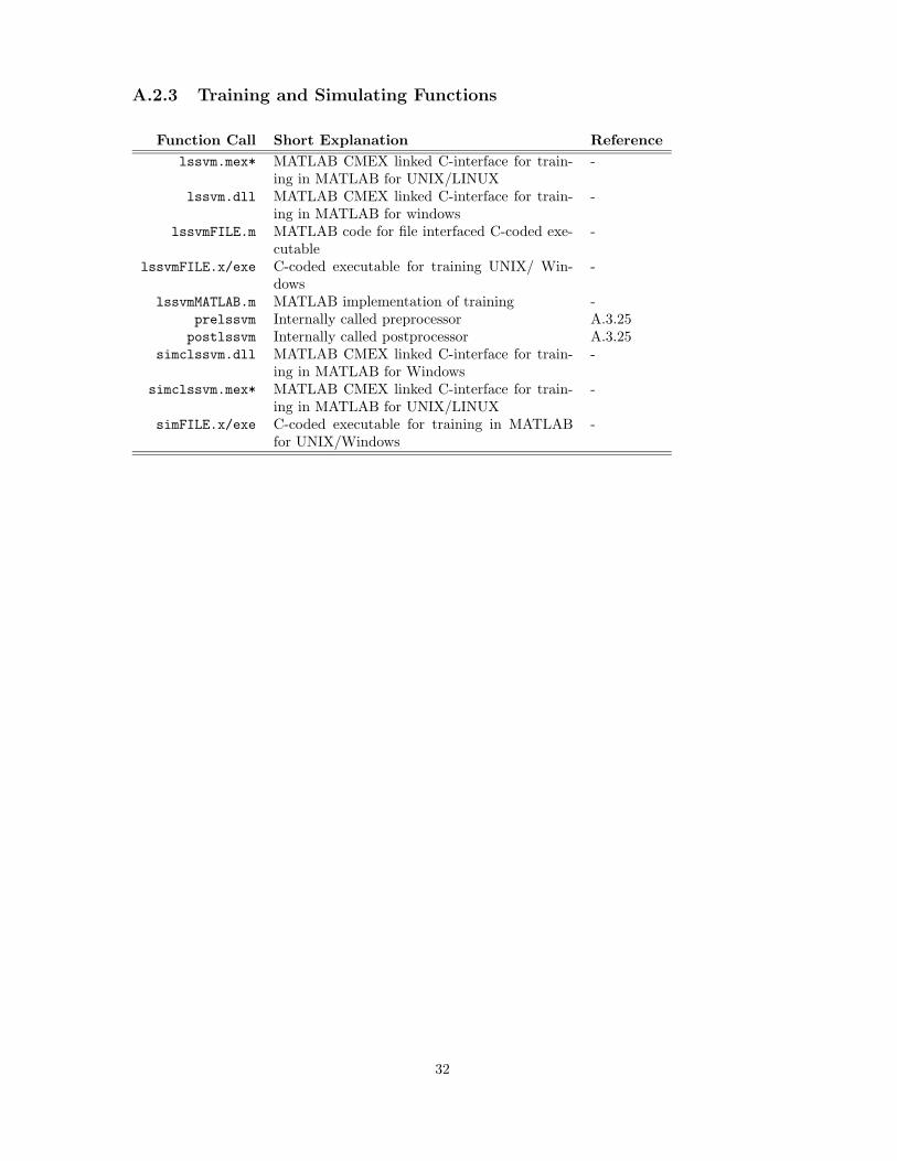
A.2.3 Training and Simulating Functions


lssvm.mex* MATLAB CMEX linked C-interface for train-ing in MATLAB for UNIX/LINUX

-

lssvm.dll MATLAB CMEX linked C-interface for train-ing in MATLAB for windows

-

lssvmFILE.m MATLAB code for file interfaced C-coded exe-cutable

-

lssvmFILE.x/exe C-coded executable for training UNIX/ Win-dows

-

lssvmMATLAB.m MATLAB implementation of training -prelssvm Internally called preprocessor A.3.25postlssvm Internally called postprocessor A.3.25

simclssvm.dll MATLAB CMEX linked C-interface for train-ing in MATLAB for Windows

-

simclssvm.mex* MATLAB CMEX linked C-interface for train-ing in MATLAB for UNIX/LINUX

-

simFILE.x/exe C-coded executable for training in MATLABfor UNIX/Windows

-

32

A.2.4 Kernel Functions


lin_kernel Linear kernel for MATLAB implementation A.3.21MLP_kernel Multilayer Perceptron kernel for MATLAB im-

plementationA.3.21

poly_kernel Polynomial kernel for MATLAB implementa-tion

A.3.21

RBF_kernel Radial Basis Function kernel for MATLAB im-plementation

A.3.21

33

A.2.5 Tuning, Sparseness and Robustness


crossvalidate Estimate the model performance with L-foldcrossvalidation

A.3.10

rcrossvalidate Estimate the model performance with robustL-fold crossvalidation

A.3.26

gridsearch A two-dimensional minimization procedurebased on exhaustive search in a limited range

A.3.33

leaveoneout Estimate the model performance with leave-one-out crossvalidation

A.3.19

leaveoneout_lssvm Fast leave-one-out cross-validation for the LS-SVM based on one full matrix inversion

A.3.20

mae, medae L1 cost measures of the residuals A.3.22linf, misclass L∞ and L0 cost measures of the residuals A.3.22

mse, trimmedmse L2 cost measures of the residuals A.3.22sparselssvm Remove iteratively the least relevant support

vectors to obtain sparsityA.3.31

tunelssvm Tune the hyperparameters of the model withrespect to the given performance measure

A.3.33

robustlssvm Robust training in the case of non-Gaussiannoise or outliers

A.3.28

validate Validate a trained model on a fixed validationset

A.3.34

34

A.2.6 Classification Extensions


code Encode and decode a multi-class classificationtask to multiple binary classifiers

A.3.9

code_ECOC Error correcting output coding A.3.9code_MOC Minimum Output Coding A.3.9

code_OneVsAll One versus All encoding A.3.9code_OneVsOne One versus One encoding A.3.9

codedist_hamming Hamming distance measure between two en-coded class labels

A.3.9

codelssvm Encoding the LS-SVM model A.3.9deltablssvm Bias term correction for the LS-SVM classifi-

catierA.3.11

roc Receiver Operating Characteristic curve of a bi-nary classifier

A.3.29

35

A.2.7 Bayesian Framework


bay_errorbar Compute the error bars for a one dimensionalregression problem

A.3.2

bay_initlssvm Initialize the hyperparameters for Bayesian in-ference

A.3.3

bay_lssvm Compute the posterior cost for the different lev-els in Bayesian inference

A.3.4

bay_lssvmARD Automatic Relevance Determination of the in-puts of the LS-SVM

A.3.5

bay_modoutClass Estimate the posterior class probabilities of abinary classifier using Bayesian inference

A.3.6

bay_optimize Optimize model- or hyperparameters with re-spect to the different inference levels

A.3.7

bay_rr Bayesian inference for linear ridge regression A.3.8eign Find the principal eigenvalues and eigenvectors

of a matrix with Nystrom’s low rank approxi-mation method

A.3.13

kernel_matrix Construct the positive (semi-) definite kernelmatrix

A.3.16

kpca Kernel Principal Component Analysis A.3.17ridgeregress Linear ridge regression A.3.27

36

A.2.8 NARX models and Prediction


predict Iterative prediction of a trained LS-SVMNARX model (in recurrent mode)

A.3.24

windowize Rearrange the data points into a Hankel matrixfor (N)AR time-series modeling

A.3.35

windowize_NARX Rearrange the input and output data intoa (block) Hankel matrix for (N)AR(X) time-series modeling

A.3.35

37

A.2.9 Unsupervised learning


AFE Automatic Feature Extraction from Nystrommethod

A.3.1

denoise_kpca Reconstruct the data mapped on the principalcomponents

A.3.12

kentropy Quadratic Renyi Entropy for a kernel based es-timator

A.3.15

kpca Compute the nonlinear kernel principal compo-nents of the data

A.3.17

38

A.2.10 Fixed Size LS-SVM

The idea of fixed size LS-SVM is still under development. However, in order to enable the userto explore this technique a number of related functions are included in the toolbox. A demoillustrates how to combine these in order to build a fixed size LS-SVM.


AFE Automatic Feature Extraction from Nystrommethod

A.3.1

bay_rr Bayesian inference of the cost on the 3 levels oflinear ridge regression

A.3.8

demo_fixedsize Demo illustrating the use of fixed size LS-SVMsfor regression

-

demo_fixedclass Demo illustrating the use of fixed size LS-SVMsfor classification

-

kentropy Quadratic Renyi Entropy for a kernel based es-timator

A.3.15

ridgeregress Linear ridge regression A.3.27

39

A.2.11 Demos

name of the demo Short Explanation

demofun Simple demo illustrating the use of LS-SVMlabfor regression

demo_fixedsize Demo illustrating the use of fixed size LS-SVMsfor regression

democlass Simple demo illustrating the use of LS-SVMlabfor classification

demo_fixedclass Demo illustrating the use of fixed size LS-SVMsfor classification

demomodel Simple demo illustrating the use of the objectoriented interface of LS-SVMlab

demo_yinyang Demo illustrating the possibilities of unsuper-vised learning by kernel PCA

40

A.3 Alphabetical List of Function Calls

A.3.1 AFE

Purpose

Automatic Feature Extraction by Nystrom method

Basic syntax

>> features = AFE(X, kernel, sig2, Xt)

Description

Using the Nystrom approximation method, the mapping of data to the feature space can beevaluated explicitly. This gives the features that one can use for a linear regression or classification.The decomposition of the mapping to the feature space relies on the eigenvalue decomposition ofthe kernel matrix. The Matlab (’eigs’) or Nystrom’s (’eign’) approximation using the nb mostimportant eigenvectors/eigenvalues can be used. The eigenvalue decomposition is not re-calculatedif it is passed as an extra argument. This routine internally calls a cmex file.

Full syntax

>> [features, U, lam] = AFE(X, kernel, sig2, Xt)

>> [features, U, lam] = AFE(X, kernel, sig2, Xt, etype)

>> [features, U, lam] = AFE(X, kernel, sig2, Xt, etype, nb)

>> features = AFE(X, kernel, sig2, Xt, [],[], U, lam)

Outputsfeatures Nt×nb matrix with extracted featuresU(*) N×nb matrix with eigenvectorslam(*) nb×1 vector with eigenvalues

InputsX N×d matrix with input datakernel Name of the used kernel (e.g. ’RBF_kernel’)sig2 Kernel parameter(s) (for linear kernel, use [])Xt Nt×d data from which the features are extractedetype(*) ’eig’(*), ’eigs’ or ’eign’nb(*) Number of eigenvalues/eigenvectors used in the eigenvalue de-

composition approximationU(*) N×nb matrix with eigenvectorslam(*) nb×1 vector with eigenvalues

See also:

kernel_matrix, RBF_kernel, demo_fixedsize

41

A.3.2 bay errorbar

Purpose

Compute the error bars for a one dimensional regression problem

Basic syntax

>> sig_e = bay_errorbar({X,Y,’function’,gam,sig2}, Xt)

>> sig_e = bay_errorbar(model, Xt)

Description

The computation takes into account the estimated noise variance and the uncertainty of the modelparameters, estimated by Bayesian inference. sig_e is the estimated standard deviation of theerror bars of the points Xt. A plot is obtained by replacing Xt by the string ’figure’.

Full syntax

• Using the functional interface:

>> sig_e = bay_errorbar({X,Y,’function’,gam,sig2,kernel,preprocess}, Xt)

>> sig_e = bay_errorbar({X,Y,’function’,gam,sig2,kernel,preprocess}, Xt, etype)

>> sig_e = bay_errorbar({X,Y,’function’,gam,sig2,kernel,preprocess}, Xt, etype, nb)

>> sig_e = bay_errorbar({X,Y,’function’,gam,sig2,kernel,preprocess}, ’figure’)

>> sig_e = bay_errorbar({X,Y,’function’,gam,sig2,kernel,preprocess}, ’figure’, etype, nb)

Outputssig_e Nt×1 vector with the σ2 errorbands of the test data

InputsX N×d matrix with the inputs of the training dataY N×1 vector with the inputs of the training datatype ’function estimation’ (’f’)gam Regularization parametersig2 Kernel parameterkernel(*) Kernel type (by default ’RBF_kernel’)preprocess(*) ’preprocess’(*) or ’original’Xt Nt×d matrix with the inputs of the test dataetype(*) ’svd’(*), ’eig’, ’eigs’ or ’eign’nb(*) Number of eigenvalues/eigenvectors used in the eigenvalue de-

composition approximation

• Using the object oriented interface:

>> [sig_e, bay, model] = bay_errorbar(model, Xt)

>> [sig_e, bay, model] = bay_errorbar(model, Xt, etype)

>> [sig_e, bay, model] = bay_errorbar(model, Xt, etype, nb)

>> [sig_e, bay, model] = bay_errorbar(model, ’figure’)

>> [sig_e, bay, model] = bay_errorbar(model, ’figure’, etype)

>> [sig_e, bay, model] = bay_errorbar(model, ’figure’, etype, nb)

42

Outputssig_e Nt×1 vector with the σ2 errorbands of the test datamodel(*) Object oriented representation of the LS-SVM modelbay(*) Object oriented representation of the results of the Bayesian

inferenceInputs

model Object oriented representation of the LS-SVM modelXt Nt×d matrix with the inputs of the test dataetype(*) ’svd’(*), ’eig’, ’eigs’ or ’eign’nb(*) Number of eigenvalues/eigenvectors used in the eigenvalue de-


See also:

bay_lssvm, bay_optimize, bay_modoutClass, plotlssvm

43

A.3.3 bay initlssvm

Purpose

Initialize the hyperparameters γ and σ2 before optimization with bay_optimize

Basic syntax

>> [gam, sig2] = bay_initlssvm({X,Y,type,[],[]})

>> model = bay_initlssvm(model)

Description

A starting value for σ2 is only given if the model has kernel type ’RBF_kernel’.

Full syntax


>> [gam, sig2] = bay_initlssvm({X,Y,type,[],[],kernel})

Outputsgam Proposed initial regularization parametersig2 Proposed initial ’RBF_kernel’ parameter

InputsX N×d matrix with the inputs of the training dataY N×1 vector with the outputs of the training datatype ’function estimation’ (’f’) or ’classifier’ (’c’)kernel(*) Kernel type (by default ’RBF_kernel’)


>> model = bay_initlssvm(model)

Outputsmodel Object oriented representation of the LS-SVM model with initial

hyperparametersInputs

model Object oriented representation of the LS-SVM model

See also:

bay_lssvm, bay_optimize

44

A.3.4 bay lssvm

Purpose

Compute the posterior cost for the 3 levels in Bayesian inference

Basic syntax

>> cost = bay_lssvm({X,Y,type,gam,sig2}, level, etype)

>> cost = bay_lssvm(model , level, etype)

Description

Estimate the posterior probabilities of model (hyper-) parameters on the different inference levels.By taking the negative logarithm of the posterior and neglecting all constants, one obtains thecorresponding cost.

Computation is only feasible for one dimensional output regression and binary classificationproblems. Each level has its different in- and output syntax:

• First level: The cost associated with the posterior of the model parameters (support valuesand bias term) is determined. The type can be:

– ’train’: do a training of the support values using trainlssvm. The total cost, thecost of the residuals (Ed) and the regularization parameter (Ew) are determined by thesolution of the support values

– ’retrain’: do a retraining of the support values using trainlssvm

– the cost terms can also be calculated from an (approximate) eigenvalue decompositionof the kernel matrix: ’svd’, ’eig’, ’eigs’ or Nystrom’s ’eign’

• Second level: The cost associated with the posterior of the regularization parameter iscomputed. The etype can be ’svd’, ’eig’, ’eigs’ or Nystrom’s ’eign’.

• Third level: The cost associated with the posterior of the chosen kernel and kernel param-eters is computed. The etype can be: ’svd’, ’eig’, ’eigs’ or Nystrom’s ’eign’.

Full syntax

• Outputs on the first level

>> [costL1,Ed,Ew,bay] = bay_lssvm({X,Y,type,gam,sig2,kernel,preprocess}, 1)

>> [costL1,Ed,Ew,bay] = bay_lssvm({X,Y,type,gam,sig2,kernel,preprocess}, 1, etype)

>> [costL1,Ed,Ew,bay] = bay_lssvm({X,Y,type,gam,sig2,kernel,preprocess}, 1, etype, nb)

>> [costL1,Ed,Ew,bay] = bay_lssvm(model, 1)

>> [costL1,Ed,Ew,bay] = bay_lssvm(model, 1, etype)

>> [costL1,Ed,Ew,bay] = bay_lssvm(model, 1, etype, nb)

With

costL1 Cost proportional to the posteriorEd(*) Cost of the fitting error termEw(*) Cost of the regularization parameterbay(*) Object oriented representation of the results of the Bayesian

inference

• Outputs on the second level

45

>> [costL2,DcostL2, optimal_cost, bay] = ...

bay_lssvm({X,Y,type,gam,sig2,kernel,preprocess}, 2, etype, nb)

>> [costL2,DcostL2, optimal_cost, bay] = bay_lssvm(model, 2, etype, nb)

With

costL2 Cost proportional to the posterior on the second levelDcostL2(*) Derivative of the costoptimal_cost(*) Optimality of the regularization parameter (optimal = 0)bay(*) Object oriented representation of the results of the Bayesian

inference

• Outputs on the third level

>> [costL3,bay] = bay_lssvm({X,Y,type,gam,sig2,kernel,preprocess}, 3, etype, nb)

>> [costL3,bay] = bay_lssvm(model, 3, etype, nb)

With

costL3 Cost proportional to the posterior on the third levelbay(*) Object oriented representation of the results of the Bayesian

inference

• Inputs using the functional interface

>> bay_lssvm({X,Y,type,gam,sig2,kernel,preprocess}, level, etype, nb)

X N×d matrix with the inputs of the training dataY N×1 vector with the outputs of the training datatype ’function estimation’ (’f’) or ’classifier’ (’c’)gam Regularization parametersig2 Kernel parameter(s) (for linear kernel, use [])kernel(*) Kernel type (by default ’RBF_kernel’)preprocess(*) ’preprocess’(*) or ’original’level 1, 2, 3etype(*) ’svd’(*), ’eig’, ’eigs’, ’eign’nb(*) Number of eigenvalues/eigenvectors used in the eigenvalue de-


• Inputs using the object oriented interface

>> bay_lssvm(model, level, etype, nb)

model Object oriented representation of the LS-SVM modellevel 1, 2, 3etype(*) ’svd’(*), ’eig’, ’eigs’, ’eign’nb(*) Number of eigenvalues/eigenvectors used in the eigenvalue de-


See also:

bay_lssvmARD, bay_optimize, bay_modoutClass, bay_errorbar

46

A.3.5 bay lssvmARD

Purpose

Bayesian Automatic Relevance Determination of the inputs of an LS-SVM

Basic syntax

>> dimensions = bay_lssvmARD({X,Y,type,gam,sig2})

>> dimensions = bay_lssvmARD(model)

Description

For a given problem, one can determine the most relevant inputs for the LS-SVM within theBayesian evidence framework. To do so, one assigns a different weighting parameter to eachdimension in the kernel and optimizes this using the third level of inference. According to theused kernel, one can remove inputs corresponding the larger or smaller kernel parameters. Thisroutine only works with the ’RBF_kernel’ with a sig2 per input. In each step, the input withthe largest optimal sig2 is removed (backward selection). For every step, the generalizationperformance is approximated by the cost associated with the third level of Bayesian inference.

The ARD is based on backward selection of the inputs based on the sig2s corresponding ineach step with a minimal cost criterion. Minimizing this criterion can be done by ’continuous’ orby ’discrete’. The former uses in each step continuous varying kernel parameter optimization,the latter decides which one to remove in each step by binary variables for each component (thiscan only applied for rather low dimensional inputs as the number of possible combinations growsexponentially with the number of inputs). If working with the ’RBF_kernel’, the kernel parameteris rescaled appropriately after removing an input variable.

The computation of the Bayesian cost criterion can be based on the singular value decompo-sition ’svd’ of the full kernel matrix or by an approximation of these eigenvalues and vectors bythe ’eigs’ or ’eign’ approximation based on ’nb’ data points.

Full syntax


>> [dimensions, ordered, costs, sig2s] = ...

bay_lssvmARD({X,Y,type,gam,sig2,kernel,preprocess}, method, etype, nb)

Outputsdimensions r×1 vector of the relevant inputsordered(*) d×1 vector with inputs in decreasing order of relevancecosts(*) Costs associated with third level of inference in every selection

stepsig2s(*) Optimal kernel parameters in each selection step

InputsX N×d matrix with the inputs of the training dataY N×1 vector with the outputs of the training datatype ’function estimation’ (’f’) or ’classifier’ (’c’)gam Regularization parametersig2 Kernel parameter(s) (for linear kernel, use [])kernel(*) Kernel type (by default ’RBF_kernel’)preprocess(*) ’preprocess’(*) or ’original’method(*) ’discrete’(*) or ’continuous’etype(*) ’svd’(*), ’eig’, ’eigs’, ’eign’nb(*) Number of eigenvalues/eigenvectors used in the eigenvalue de-


47


>> [dimensions, ordered, costs, sig2s, model] = bay_lssvmARD(model, method, etype, nb)

Outputsdimensions r×1 vector of the relevant inputsordered(*) d×1 vector with inputs in decreasing order of relevancecosts(*) Costs associated with third level of inference in every selection

stepsig2s(*) Optimal kernel parameters in each selection stepmodel(*) Object oriented representation of the LS-SVM model trained

only on the relevant inputsInputs

model Object oriented representation of the LS-SVM modelmethod(*) ’discrete’(*) or ’continuous’etype(*) ’svd’(*), ’eig’, ’eigs’, ’eign’nb(*) Number of eigenvalues/eigenvectors used in the eigenvalue de-


See also:

bay_lssvm, bay_optimize, bay_modoutClass, bay_errorbar

48

A.3.6 bay modoutClass

Purpose

Estimate the posterior class probabilities of a binary classifier using Bayesian inference

Basic syntax

>> [Ppos, Pneg] = bay_modoutClass({X,Y,’classifier’,gam,sig2}, Xt)

>> [Ppos, Pneg] = bay_modoutClass(model, Xt)

Description

Calculate the probability that a point will belong to the positive or negative classes taking intoaccount the uncertainty of the parameters. Optionally, one can express prior knowledge as aprobability between 0 and 1, where prior equal to 2/3 means that the prior positive class probabilityis 2/3 (more likely to occur than the negative class).

For binary classification tasks with a 2 dimensional input space, one can make a surface plotby replacing Xt by the string ’figure’.

Full syntax


>> [Ppos, Pneg] = bay_modoutClass({X,Y,’classifier’,...

\ gam,sig2, kernel, preprocess}, Xt)


gam,sig2, kernel, preprocess}, Xt, prior)


gam,sig2, kernel, preprocess}, Xt, prior, etype)


gam,sig2, kernel, preprocess}, Xt, prior, etype, nb)

>> bay_modoutClass({X,Y,’classifier’,...

gam,sig2, kernel, preprocess}, ’figure’)


gam,sig2, kernel, preprocess}, ’figure’, prior)


gam,sig2, kernel, preprocess}, ’figure’, prior, etype)


gam,sig2, kernel, preprocess}, ’figure’, prior, etype, nb)

49

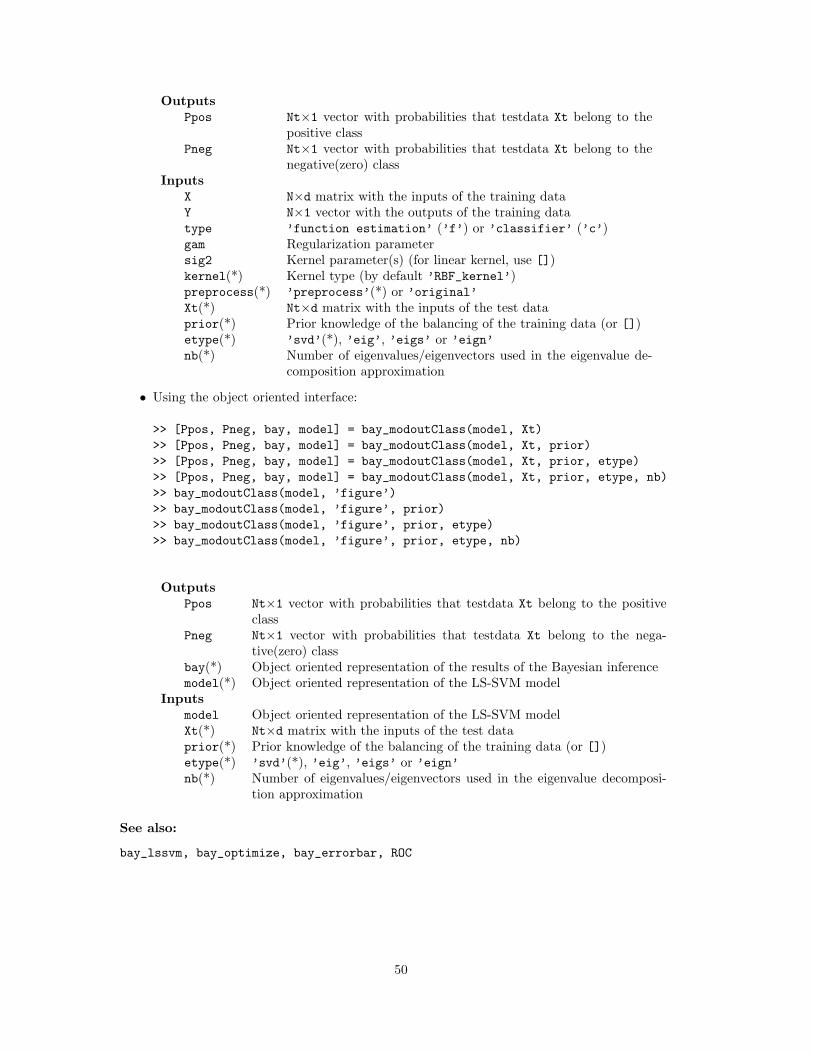
OutputsPpos Nt×1 vector with probabilities that testdata Xt belong to the

positive classPneg Nt×1 vector with probabilities that testdata Xt belong to the

negative(zero) classInputs

X N×d matrix with the inputs of the training dataY N×1 vector with the outputs of the training datatype ’function estimation’ (’f’) or ’classifier’ (’c’)gam Regularization parametersig2 Kernel parameter(s) (for linear kernel, use [])kernel(*) Kernel type (by default ’RBF_kernel’)preprocess(*) ’preprocess’(*) or ’original’Xt(*) Nt×d matrix with the inputs of the test dataprior(*) Prior knowledge of the balancing of the training data (or [])etype(*) ’svd’(*), ’eig’, ’eigs’ or ’eign’nb(*) Number of eigenvalues/eigenvectors used in the eigenvalue de-



>> [Ppos, Pneg, bay, model] = bay_modoutClass(model, Xt)

>> [Ppos, Pneg, bay, model] = bay_modoutClass(model, Xt, prior)

>> [Ppos, Pneg, bay, model] = bay_modoutClass(model, Xt, prior, etype)

>> [Ppos, Pneg, bay, model] = bay_modoutClass(model, Xt, prior, etype, nb)

>> bay_modoutClass(model, ’figure’)

>> bay_modoutClass(model, ’figure’, prior)

>> bay_modoutClass(model, ’figure’, prior, etype)

>> bay_modoutClass(model, ’figure’, prior, etype, nb)

OutputsPpos Nt×1 vector with probabilities that testdata Xt belong to the positive

classPneg Nt×1 vector with probabilities that testdata Xt belong to the nega-

tive(zero) classbay(*) Object oriented representation of the results of the Bayesian inferencemodel(*) Object oriented representation of the LS-SVM model

Inputsmodel Object oriented representation of the LS-SVM modelXt(*) Nt×d matrix with the inputs of the test dataprior(*) Prior knowledge of the balancing of the training data (or [])etype(*) ’svd’(*), ’eig’, ’eigs’ or ’eign’nb(*) Number of eigenvalues/eigenvectors used in the eigenvalue decomposi-

tion approximation

See also:

bay_lssvm, bay_optimize, bay_errorbar, ROC

50

A.3.7 bay optimize

Purpose

Optimize the posterior probabilities of model (hyper-) parameters with respect to the different levelsin Bayesian inference

Basic syntax

One can optimize on the three different inference levels as described in section 2.1.3.

• First level: In the first level one optimizes the support values α’s and the bias b.

• Second level: In the second level one optimizes the regularization parameter gam.

• Third level: In the third level one optimizes the kernel parameter. In the case of thecommon ’RBF_kernel’ the kernel parameter is the bandwidth sig2.

This routine is only tested with Matlab version 6 using the corresponding optimization toolbox.

Full syntax

• Outputs on the first level:

>> [model, alpha, b] = bay_optimize({X,Y,type,gam,sig2,kernel,preprocess}, 1)

>> [model, alpha, b] = bay_optimize(model, 1)

With

model Object oriented representation of the LS-SVM model optimized on thefirst level of inference

alpha(*) Support values optimized on the first level of inferenceb(*) Bias term optimized on the first level of inference

• Outputs on the second level:

>> [model,gam] = bay_optimize({X,Y,type,gam,sig2,kernel,preprocess}, 2)

>> [model,gam] = bay_optimize(model, 2)

With

model Object oriented representation of the LS-SVM model optimized on thesecond level of inference

gam(*) Regularization parameter optimized on the second level of inference

• Outputs on the third level:

>> [model, sig2] = bay_optimize({X,Y,type,gam,sig2,kernel,preprocess}, 3)

>> [model, sig2] = bay_optimize(model, 3)

With

model Object oriented representation of the LS-SVM model optimized on thethird level of inference

sig2(*) Kernel parameter optimized on the third level of inference

• Inputs using the functional interface

51

>> model = bay_optimize({X,Y,type,gam,sig2,kernel,preprocess}, level)

>> model = bay_optimize({X,Y,type,gam,sig2,kernel,preprocess}, level, etype)

>> model = bay_optimize({X,Y,type,gam,sig2,kernel,preprocess}, level, etype, nb)

X N×d matrix with the inputs of the training dataY N×1 vector with the outputs of the training datatype ’function estimation’ (’f’) or ’classifier’ (’c’)gam Regularization parametersig2 Kernel parameter(s) (for linear kernel, use [])kernel(*) Kernel type (by default ’RBF_kernel’)preprocess(*) ’preprocess’(*) or ’original’level 1, 2, 3etype(*) ’eig’, ’svd’(*), ’eigs’, ’eign’nb(*) Number of eigenvalues/eigenvectors used in the eigenvalue decomposi-

tion approximation

• Inputs using the object oriented interface

>> model = bay_optimize(model, level)

>> model = bay_optimize(model, level, etype)

>> model = bay_optimize(model, level, etype, nb)

model Object oriented representation of the LS-SVM modellevel 1, 2, 3etype(*) ’eig’, ’svd’(*), ’eigs’, ’eign’nb(*) Number of eigenvalues/eigenvectors used in the eigenvalue decomposi-

tion approximation

See also:

bay_lssvm, bay_lssvmARD, bay_modoutClass, bay_errorbar

52

A.3.8 bay rr

Purpose

Bayesian inference of the cost on the three levels of linear ridge regression

Basic syntax

>> cost = bay_rr(X, Y, gam, level)

Description

This function implements the cost functions related to the Bayesian framework of linear ridgeRegression [29]. Optimizing this criteria results in optimal model parameters W,b, hyperparameters.The criterion can also be used for model comparison.

The obtained model parameters w and b are optimal on the first level w.r.t J = 0.5*w’*w+gam*0.5*sum(Y-X*w-b).^2.

Full syntax

• Outputs on the first level: Cost proportional to the posterior of the model parameters.

>> [costL1, Ed, Ew] = bay_rr(X, Y, gam, 1)

With

costL1 Cost proportional to the posteriorEd(*) Cost of the fitting error termEw(*) Cost of the regularization parameter

• Outputs on the second level: Cost proportional to the posterior of gam.

>> [costL2, DcostL2, Deff, mu, ksi, eigval, eigvec] = bay_rr(X, Y, gam, 2)

With

costL2 Cost proportional to the posterior on the second levelDcostL2(*) Derivative of the cost proportional to the posteriorDeff(*) Effective number of parametersmu(*) Relative importance of the fitting error termksi(*) Relative importance of the regularization parametereigval(*) Eigenvalues of the covariance matrixeigvec(*) Eigenvectors of the covariance matrix

• Outputs on the third level: The following commands can be used to compute the level3 cost function for different models (e.g. models with different selected sets of inputs). Thebest model can then be chosen as the model with best level 3 cost (CostL3).

>> [costL3, gam_optimal] = bay_rr(X, Y, gam, 3)

With

costL3 Cost proportional to the posterior on the third inference levelgam_optimal(*) Optimal regularization parameter obtained from optimizing the second

level

53

• Inputs:

>> cost = bay_rr(X, Y, gam, level)

X N×d matrix with the inputs of the training dataY N×1 vector with the outputs of the training datagam Regularization parameterlevel 1, 2, 3

See also:

ridgeregress,bay_lssvm

54

A.3.9 code, codelssvm

Purpose

Encode and decode a multi-class classification task into multiple binary classifiers

Basic syntax

>> Yc = code(Y, codebook)

Description

The coding is defined by the codebook. The codebook is represented by a matrix where thecolumns represent all different classes and the rows indicate the result of the binary classifiers.An example is given: the 3 classes with original labels [1 2 3] can be encoded in the followingcodebook (using Minimum Output Coding ):

>> codebook

= [-1 -1 1;

1 -1 1]

For this codebook, a member of the first class is found if the first binary classifier is negativeand the second classifier is positive. A don’t care is represented by eps. By default it is assumedthat the original classes are represented as different numerical labels. One can overrule this bypassing the old_codebook which contains information about the old representation.

A codebook can be created by one of the functions (codefct) code_MOC, code_OneVsOne,code_OneVsAll, code_ECOC. Additional arguments to this function can be passed as a cell incodefct_args.

>> Yc = code(Y,codefct,codefct_args)

>> Yc = code(Y,codefct,codefct_args, old_codebook)

>> [Yc, codebook, oldcodebook] = code(Y,codefct,codefct_args)

To detect the classes of a disturbed encoded signal given the corresponding codebook, oneneeds a distance function (fctdist) with optional arguments given as a cell (fctdist_args). Bydefault, the Hamming distance (of function codedist_hamming) is used.

>> Yc = code(Y, codefct, codefct_args, old_codebook, fctdist, fctdist_args)

A simple example is given here, a more elaborated example is given in section 3.1.4. Here, ashort categorical signal Y is encoded in Yec using Minimum Output Coding and decoded again toits original form:

>> Y = [1; 2; 3; 2; 1]

>> [Yc,codebook,old_codebook] = code(Y,’code_MOC’) % encode

>> Yc

= [-1 -1

-1 1

1 -1

-1 1

-1 -1]

>> codebook

= [ -1 -1 1

-1 1 -1]

>> old_codebook

= [1 2 3]

55

>> code(Yc, old_codebook, [], codebook, ’codedist_hamming’) % decode

ans

= [1; 2; 3; 2; 1]

Different encoding schemes are available:

• Minimum Output Coding (code_MOC)Here the minimal number of bits nb is used to encode the nc classes:

nb = dlog2 nce.

• Error Correcting Output Code (code_ECOC)This coding scheme uses redundant bits. Typically, one bounds the number of binary clas-sifiers nb by

nb ≤ 15dlog2 nce.

However, it is not guaranteed to have a valid nb-representation of nc classes for all combi-nations. This routine based on backtracking can take some memory and time.

• One versus All Coding (code_OneVsAll)Each binary classifier k = 1, ..., nc is trained to discriminate between class k and the unionof the others.

• One Versus One Coding (code_OneVsOns)Each of the nb binary classifiers is used to discriminate between a specific pair of nc classes

nb =nc(nc − 1)

2.

Different decoding schemes are implemented:

• Hamming Distance (codedist_hamming)This measure equals the number of corresponding bits in the binary result and the codeword.Typically, it is used for the Error Correcting Code.

• Bayesian Distance Measure (codedist_bay)The Bayesian moderated output of the binary classifiers is used to estimate the posteriorprobability.

Encoding using the previous algorithms of the LS-SVM multi-class classifier can easily be doneby codelssvm. It will be invoked by trainlssvm if an appropriate encoding scheme is defined ina model. An example shows how to use the Bayesian distance measure to extract the estimatedclass from the simulated encoded signal. Assumed are input and output data X and Y (size isrespectively Ntrain×Din and Ntrain×1), a kernel parameter sig2 and a regularization parametergam. Yt corresponding to a set of data points Xt (size is Ntest × Din) is to be estimated:

% encode for training

>> model = initlssvm(X, Y, ’classifier’, gam, sig2)

>> model = changelssvm(model, ’codetype’, ’code_MOC’)

>> model = changelssvm(model, ’codedist_fct’, ’codedist_hamming’)

>> model = codelssvm(model) % implicitly called by next command

>> model = trainlssvm(model)


% decode for simulating

>> model = changelssvm(model, ’codedist_fct’, ’codedist_bay’)

>> model = changelssvm(model, ’codedist_args’,...

{bay_modoutClass(model,Xt)})

>> Yt = simlssvm(model, Xt)

56

Full syntax

We denote the number of used binary classifiers by nbits and the number of different representedclasses by nc.

• For encoding:

>> [Yc, codebook, old_codebook] = code(Y, codefct)

>> [Yc, codebook, old_codebook] = code(Y, codefct, codefct_args)

>> Yc = code(Y, given_codebook)

OutputsYc N×nbits encoded output classifiercodebook(*) nbits*nc matrix representing the used encodingold_codebook(*) d*nc matrix representing the original encoding

InputsY N×d matrix representing the original classifiercodefct(*) Function to generate a new codebook (e.g. code_MOC)codefct_args(*) Extra arguments for codefctgiven_codebook(*) nbits*nc matrix representing the encoding to use

• For decoding:

>> Yd = code(Yc, codebook,[], old_codebook)

>> Yd = code(Yc, codebook,[], old_codebook, codedist_fct)

>> Yd = code(Yc, codebook,[], old_codebook, codedist_fct, codedist_args)

OutputsYd N×nc decoded output classifier

InputsY N×d matrix representing the original classifiercodebook d*nc matrix representing the original encodingold_codebook bits*nc matrix representing the encoding of the given classifiercodedist_fct Function to calculate the distance between to encoded classifiers (e.g.

codedist_hamming)codedist_args(*) Extra arguments of codedist_fct

See also:

code_ECOC, code_MOC, code_OneVsAll, code_OneVsOne, codedist_hamming

57

A.3.10 crossvalidate

Purpose

Estimate the model performance of a model with l-fold crossvalidation

Basic syntax

>> cost = crossvalidate({Xtrain,Ytrain,type,gam,sig2}, Xval, Yval)

>> cost = crossvalidate(model, Xval, Yval)

Description

The data is once permutated randomly, then it is divided into L (by default 10) disjunct sets.In the i-th (i = 1, ..., l) iteration, the i-th set is used to estimate the performance (’validationset’) of the model trained on the other l − 1 sets (’training set’). At last, the l (denoted by L)different estimates of the performance are combined (by default by the ’mean’). The assumptionis made that the input data are distributed independent and identically over the input space. Asadditional output, the costs in the different folds (’costs’) and all residuals (’ec’) of the data arereturned:

>> [cost, costs, ec] = crossvalidate(model, Xval, Yval)

By default, this function will call the training (trainlssvm) and simulation (simlssvm) algo-rithms for LS-SVMs. However, one can use the validation function more generically by specifyingthe appropriate training and simulation function. Some commonly used criteria are:

>> cost = crossvalidate(model, Xval, Yval, 10, ’misclass’, ’mean’, ’corrected’)

>> cost = crossvalidate(model, Xval, Yval, 10, ’mse’, ’mean’, ’original’)

>> cost = crossvalidate(model, Xval, Yval, 10, ’mae’, ’median’, ’corrected’)

Full syntax

• Using LS-SVMlab with the functional interface:

>> [cost, costs, ec] = crossvalidate({X,Y,type,gam,sig2,kernel,preprocess}, Xval, Yval)

>> [cost, costs, ec] = crossvalidate({X,Y,type,gam,sig2,kernel,preprocess}, Xval, Yval, L)

>> [cost, costs, ec] = crossvalidate({X,Y,type,gam,sig2,kernel,preprocess},...

Xval, Yval, L, estfct, combinefct)

>> [cost, costs, ec] = crossvalidate({X,Y,type,gam,sig2,kernel,preprocess},...

Xval, Yval, L, estfct, combinefct, correction)

58

Outputscost Cost estimation of the L-fold cross-validationcosts(*) L×1 vector with costs estimated on the L different foldsec(*) N×1 vector with residuals of all data

InputsX Training input data used for defining the LS-SVM and the preprocessingY Training output data used for defining the LS-SVM and the preprocess-

ingtype ’function estimation’ (’f’) or ’classifier’ (’c’)gam Regularization parametersig2 Kernel parameter(s) (for linear kernel, use [])kernel(*) Kernel type (by default ’RBF_kernel’)preprocess(*) ’preprocess’(*) or ’original’Xval N×d matrix with the inputs of the data used for cross-validationYval N×m matrix with the outputs of the data used for cross-validationL(*) Number of folds (by default 10)estfct(*) Function estimating the cost based on the residuals (by default mse)combinefct(*) Function combining the estimated costs on the different folds (by default

mean)correction(*) ’original’(*) or ’corrected’


>> [cost, costs, ec] = crossvalidate(model, Xval, Yval)

>> [cost, costs, ec] = crossvalidate(model, Xval, Yval, L)

>> [cost, costs, ec] = crossvalidate(model, Xval, Yval, L, estfct)

>> [cost, costs, ec] = crossvalidate(model, Xval, Yval, L, estfct, combinefct)

>> [cost, costs, ec] = crossvalidate(model, Xval, Yval, L, estfct, combinefct, correction)


Inputsmodel Object oriented representation of the LS-SVM modelXval Nt×d matrix with the inputs of the validation points used in the proce-

dureYval Nt×m matrix with the outputs of the validation points used in the pro-

cedureL(*) Number of folds (by default 10)estfct(*) Function estimating the cost based on the residuals (by default mse)combinefct(*) Function combining the estimated costs on the different folds (by default


• Using other modeling techniques::

>> [cost, costs, ec] = crossvalidate(model, Xval, Yval, L,...

estfct, combinefct, correction, trainfct, simfct)

59


Inputsmodel Object oriented representation of the modelXval Nt×d matrix with the inputs of the validation points usedYval Nt×m matrix with the outputs of the validation points used in the pro-

cedureL(*) Number of folds (by default 10)estfct(*) Function estimating the cost based on the residuals (by default mse)combinefct(*) Function combining the estimated costs on the different folds (by default

mean)correction(*) ’original’(*) or ’corrected’trainfct Function used to train the modelsimfct Function used to simulate test data with the model

See also:

validate, leaveoneout, leaveoneout_lssvm, trainlssvm, simlssvm

60

A.3.11 deltablssvm

Purpose

Bias term correction for the LS-SVM classifier

Basic syntax

>> model = deltablssvm(model, b_new)

Description

This function is only useful in the object oriented function interface. Set explicitly the bias termb_new of the LS-SVM model.

Full syntax

>> model = deltablssvm(model, b_new)

Outputsmodel Object oriented representation of the LS-SVM model with initial hyper-

parametersInputs

model Object oriented representation of the LS-SVM modelb_new m×1 vector with new bias term(s) for the model

See also:

roc, trainlssvm, simlssvm, changelssvm

61

A.3.12 denoise kpca

Purpose

Reconstruct the data mapped on the first principal components

Basic syntax

>> Xd = denoise_kpca(X, kernel, kernel_par);

Description

Denoising can be done by moving the point in input space so that its corresponding map to featurespace is optimized. This means that the data point in feature space is as close as possible with itscorresponding reconstructed points using the principal components. If the principal componentsare to be calculated on the same data ’X’ as the one one wants to denoise, use the command:

>> Xd = denoise_kpca(X, kernel, kernel_par);

>> [Xd,lam,U] = denoise_kpca(X, kernel, kernel_par, [], etype, nb);

When one wants to denoise data ’Xt’ other than the data used to obtain the principal components:

>> Xd = denoise_kpca(X, kernel, kernel_par, Xt);

>> [Xd, lam, U] = denoise_kpca(X, kernel, kernel_par, Xt, etype, nb);

Full syntax

• >> [Xd, lam, U] = denoise_kpca(X, kernel, kernel_par, Xt);

>> [Xd, lam, U] = denoise_kpca(X, kernel, kernel_par, Xt, etype);

>> [Xd, lam, U] = denoise_kpca(X, kernel, kernel_par, Xt, etype, nb);

OutputsXd N×d (Nt×d) matrix with denoised data X (Xt)lam(*) nb×1 vector with eigenvalues of principal componentsU(*) N×nb (Nt×d) matrix with principal eigenvectors

InputsX N×d matrix with data points used for finding the principal componentskernel Kernel type (e.g. ’RBF_kernel’)kernel_par Kernel parameter(s) (for linear kernel, use [])Xt(*) Nt×d matrix with the points to denoise (if not specified, X is denoised

instead)etype(*) ’eig’(*), ’svd’, ’eigs’, ’eign’nb(*) Number of principal components used in approximation

• >> Xd = denoise_kpca(X, U, lam, kernel, kernel_par, Xt);

OutputsXd N×d (Nt×d) matrix with denoised data X (Xt)

InputsX N×d matrix with data points used for finding the principal componentsU N×nb (Nt×d) matrix with principal eigenvectorslam nb×1 vector with eigenvalues of principal componentskernel Kernel type (e.g. ’RBF_kernel’)kernel_par Kernel parameter(s) (for linear kernel, use [])Xt(*) Nt×d matrix with the points to denoise (if not specified, X is denoised

instead)

62

See also:

kpca, kernel_matrix, RBF_kernel

63

A.3.13 eign

Purpose

Find the principal eigenvalues and eigenvectors of a matrix with Nystrom’s low rank approximationmethod

Basic syntax

>> D = eign(A, nb)

>> [V, D] = eign(A, nb)

Description

In the case of using this method for low rank approximation and decomposing the kernel matrix,one can call the function without explicit construction of the matrix A.

>> D = eign(X, kernel, kernel_par, nb)

>> [V, D] = eign(X, kernel, kernel_par, nb)

Full syntax

We denote the size of positive definite matrix A with a*a.

• Given the full matrix:

>> D = eign(A,nb)

>> [V,D] = eign(A,nb)

OutputsV(*) a×nb matrix with estimated principal eigenvectors of AD nb×1 vector with principal estimated eigenvalues of A

InputsA a*a positive definite symmetric matrixnb(*) Number of approximated principal eigenvalues/eigenvectors

• Given the function to calculate the matrix elements:

>> D = eign(X, kernel, kernel_par, n)

>> [V,D] = eign(X, kernel, kernel_par, n)

OutputsV(*) a×nb matrix with estimated principal eigenvectors of AD nb×1 vector with estimated principal eigenvalues of A

InputsX N×d matrix with the training datakernel Kernel type (e.g. ’RBF_kernel’)kernel_par Kernel parameter(s) (for linear kernel, use [])nb(*) Number of eigenvalues/eigenvectors used in the eigenvalue decomposi-

tion approximation

See also:

eig, eigs, kpca, bay_lssvm

64

A.3.14 initlssvm, changelssvm

Purpose

Only for use with the object oriented model interface

Description

The Matlab toolbox interface is organized in two equivalent ways. In the functional way, func-tion calls need explicit input and output arguments. An advantage is their similarity with themathematical equations.

An alternative syntax is based on the concept of a model, gathering all the relevant signals,parameters and algorithm choices. The model is initialized by model=initlssvm(...), or will beinitiated implicitly by passing the arguments of initlssvm(...) in one cell as the argument ofthe LS-SVM specific functions, e.g. for training:

>> model = trainlssvm({X,Y,type,gam,sig2})

...

>> model = changelssvm(model,’field’,’value’)

After training, the model contains the solution of the training including the used default values. Allcontents of the model can be requested (model.<contenttype>) or changed (changelssvm) eachmoment. The user is advised not to change the fields of the model by model.<field>=<value>

as the toolbox cannot guarantee consistency anymore in this way.The different options are given in following table:

• General options representing the kind of model:

type: ’classifier’ ,’function estimation’

implementation: ’CMEX’ ,’CFILE’ ,’MATLAB’

status: Status of this model (’trained’ or ’changed’ )

alpha: Support values of the trained LS-SVM model

b: Bias term of the trained LS-SVM model

duration: Number of seconds the training lasts

latent: Returning latent variables (’no’ ,’yes’ )

x_delays: Number of delays of eXogeneous variables (by default 0 )

y_delays: Number of delays of responses (by default 0 )

steps: Number of steps to predict (by default 1 )

gam: Regularisation parameter

kernel_type: Kernel function

kernel_pars: Extra parameters of the kernel function

• Fields used to specify the used training data:

x_dim: Dimension of input space

y_dim: Dimension of responses

nb_data: Number of training data

xtrain: (preprocessed) inputs of training data

ytrain: (preprocessed,coded) outputs of training data

selector: Indexes of training data effectively used during training

• Options used in the Conjugate Gradient (CG) algorithm:

65

cga_max_itr: Maximum number of iterations in CG

cga_eps: Stopcriterium of CG, largest allowed error

cga_fi_bound: Stopcriterium of CG, smallest allowed improvement

cga_show: Show the results of the CG algorithm (1 or 0)

cga_startvalues: Starting values of the CG algorithm

• Fields with the information for pre- and post-processing (only given if appropriate):

preprocess: ’preprocess’ or ’original’

schemed: Status of the preprocessing

(’coded’ ,’original’ or ’schemed’ )

pre_xscheme: Scheme used for preprocessing the input data

pre_yscheme: Scheme used for preprocessing the output data

pre_xmean: Mean of the input data

pre_xstd: Standard deviation of the input data

pre_ymean: Mean of the responses

pre_ystd: Standard deviation of the reponses

• The specifications of the used encoding (only given if appropriate):

code: Status of the coding

(’original’ ,’changed’ or ’encoded’)

codetype: Used function for constructing the encoding

for multiclass classification (by default ’none’)

codetype_args: Arguments of the codetype function

codedist_fct: Function used to calculate to which class a

coded result belongs

codedist_args: Arguments of the codedist function

codebook2: Codebook of the new coding

codebook1: Codebook of the original coding

Full syntax

• >> model = initlssvm(X, Y, type, gam, sig2, kernel, preprocess)

Outputsmodel Object oriented representation of the LS-SVM model

InputsX N×d matrix with the inputs of the training dataY N×1 vector with the outputs of the training datatype ’function estimation’ (’f’) or ’classifier’ (’c’)gam Regularization parametersig2 Kernel parameter(s) (for linear kernel, use [])kernel(*) Kernel type (by default ’RBF_kernel’)preprocess(*) ’preprocess’(*) or ’original’implementation(*) ’CMEX’(*), ’CFILE’ or ’MATLAB’

• >> model = changelssvm(model, field, value)

66

Outputsmodel(*) Obtained object oriented representation of the LS-SVM model

Inputsmodel Original object oriented representation of the LS-SVM modelfield Field of the model one wants to change (e.g. ’preprocess’)value New value of the field of the model one wants to change

See also:

trainlssvm, initlssvm, simlssvm, plotlssvm.

67

A.3.15 kentropy

Purpose

Quadratic Renyi Entropy for a kernel based estimator

Basic syntax

Given the eigenvectors and the eigenvalues of the kernel matrix, the entropy is computed by

>> H = kentropy(X, U, lam)

The eigenvalue decomposition can also be computed (or approximated) implicitly:

>> H = kentropy(X, kernel, sig2)

Full syntax

• >> H = kentropy(X, kernel, kernel_par)

>> H = kentropy(X, kernel, kernel_par, etype)

>> H = kentropy(X, kernel, kernel_par, etype, nb)

OutputsH Quadratic Renyi entropy of the kernel matrix

InputsX N×d matrix with the training datakernel Kernel type (e.g. ’RBF_kernel’)kernel_par Kernel parameter(s) (for linear kernel, use [])etype(*) ’eig’(*), ’eigs’, ’eign’nb(*) Number of eigenvalues/eigenvectors used in the eigenvalue decomposi-

tion approximation

• >> H = kentropy(X, U, lam)

OutputsH Quadratic Renyi entropy of the kernel matrix

InputsX N×d matrix with the training dataU N×nb matrix with principal eigenvectorslam nb×1 vector with eigenvalues of principal components

See also:

kernel_matrix, demo_fixedsize, RBF_kernel

68

A.3.16 kernel matrix

Purpose

Construct the positive (semi-) definite and symmetric kernel matrix

Basic Syntax

>> Omega = kernel_matrix(X, kernel_fct, sig2)

Description

This matrix should be positive definite if the kernel function satisfies the Mercer condition. Con-struct the kernel values for all test data points in the rows of Xt, relative to the points of X.

>> Omega_Xt = kernel_matrix(X, kernel_fct, sig2, Xt)

Full syntax

>> Omega = kernel_matrix(X, kernel_fct, sig2)

>> Omega = kernel_matrix(X, kernel_fct, sig2, Xt)

OutputsOmega N×N (N×Nt) kernel matrix

InputsX N×d matrix with the inputs of the training datakernel Kernel type (by default ’RBF_kernel’)sig2 Kernel parameter(s) (for linear kernel, use [])Xt(*) Nt×d matrix with the inputs of the test data

See also:

RBF_kernel, lin_kernel, kpca, trainlssvm

69

A.3.17 kpca

Purpose

Kernel Principal Component Analysis (KPCA)

Basic syntax

>> [eigval, eigvec] = kpca(X, kernel_fct, sig2)

>> [eigval, eigvec, scores] = kpca(X, kernel_fct, sig2, Xt)

Description

Compute the nb largest eigenvalues and the corresponding rescaled eigenvectors correspondingwith the principal components in the feature space of the centered kernel matrix. To calculatethe eigenvalue decomposition of this N × N matrix, Matlab’s eig is called by default. Thedecomposition can also be approximated by Matlab (’eigs’) or by Nystrom’s method (’eign’)using nb components. In some cases one wants to disable (’original’) the rescaling of theprincipal components in feature space to unit length.

The scores of a test set Xt on the principal components is computed by the call:

>> [eigval, eigvec, scores] = kpca(X, kernel_fct, sig2, Xt)

Full syntax

>> [eigval, eigvec, empty, omega] = kpca(X, kernel_fct, sig2)

>> [eigval, eigvec, empty, omega] = kpca(X, kernel_fct, sig2, [], etype)

>> [eigval, eigvec, empty, omega] = kpca(X, kernel_fct, sig2, [],etype, nb)

>> [eigval, eigvec, empty, omega] = kpca(X, kernel_fct, sig2, [],etype, nb, rescaling)

>> [eigval, eigvec, scores, omega] = kpca(X, kernel_fct, sig2, Xt)

>> [eigval, eigvec, scores, omega] = kpca(X, kernel_fct, sig2, Xt, etype)

>> [eigval, eigvec, scores, omega] = kpca(X, kernel_fct, sig2, Xt,etype, nb)

>> [eigval, eigvec, scores, omega] = kpca(X, kernel_fct, sig2, Xt,etype, nb, rescaling)

Outputseigval N (nb)×1 vector with eigenvalues valueseigvec N×N (N×nb) matrix with the principal directionsXt(*) Nt×nb matrix with the scores of the test data (or [])Omega(*) N×N centered kernel matrix

InputsX N×d matrix with the inputs of the training datakernel Kernel type (e.g. ’RBF_kernel’)sig2 Kernel parameter(s) (for linear kernel, use [])Xt(*) Nt×d matrix with the inputs of the test data (or [])etype(*) ’svd’, ’eig’(*),’eigs’,’eign’nb(*) Number of eigenvalues/eigenvectors used in the eigenvalue decomposi-

tion approximationrescaling(*) ’original size’ (’o’) or ’rescaling’(*) (’r’)

See also:

bay_lssvm, bay_optimize, eign

70

A.3.18 latentlssvm

Purpose

Calculate the latent variables of the LS-SVM classifier at the given test data

Basic syntax

>> Zt = latentlssvm({X,Y,’classifier’,gam,sig2,kernel}, {alpha,b}, Xt)

>> Zt = latentlssvm({X,Y,’classifier’,gam,sig2,kernel}, Xt)

>> [Zt, model] = latentlssvm(model, Xt)

Description

The latent variables of a binary classifier are the continuous simulated values of the test data whichare used to make the final classifications. The classification of a testpoint depends on whetherthe latent value exceeds the model’s threshold (b). If appropriate, the model is trained by thestandard procedure (trainlssvm) first.

As an application example: crossvalidation can be based on the latent variables:

>> cost = crossvalidate(model, X, Y, 10,...

’mse’, ’mean’, ’original’, ’trainlssvm’, ’latentlssvm’)

Full syntax


>> Zt = latentlssvm({X,Y,’classifier’,gam,sig2,kernel}, {alpha,b}, Xt)

>> Zt = latentlssvm({X,Y,type,gam,sig2,kernel,preprocess}, Xt)

OutputsZt Nt×m matrix with predicted latent simulated outputs

InputsX N×d matrix with the inputs of the training dataY N×m vector with the outputs of the training datatype ’classifier’ (’c’)gam Regularization parametersig2 Kernel parameter(s) (for linear kernel, use [])kernel(*) Kernel type (by default ’RBF_kernel’)preprocess(*) ’preprocess’(*) or ’original’alpha(*) N×1 matrix with the support valuesb(*) the bias termsXt Nt×d matrix with the inputs of the test data


>> [Zt, model] = latentlssvm(model, Xt)

OutputsZt Nt×m matrix with continuous latent simulated outputsmodel(*) Trained object oriented representation of the LS-SVM model

Inputsmodel Object oriented representation of the LS-SVM modelXt Nt×d matrix with the inputs of the test data

71

See also:

trainlssvm, simlssvm.

81

A.3.24 predict

Purpose

Iterative prediction of a trained LS-SVM NARX model (in recurrent mode)

Description

>> Yp = predict({Xw,Yw,type,gam,sig2}, Xt, nb)

>> Yp = predict(model, Xt, nb)

Description

The model needs to be trained using Xw, Yw which is the result of windowize or windowizeNARX.The number of time lags for the model is determined by the dimension of the input, or if notappropriate, by the number of given starting values.

By default, the model is evaluated on the past points using simlssvm. However, if one wantsto use this procedure for other models, this default can be overwritten by your favorite trainingfunction. This function (denoted by simfct) has to follow the following syntax:

>> simfct(model,inputs,arguments)

thus:

>> Yp = predict(model, Xt, nb, simfct)

>> Yp = predict(model, Xt, nb, simfct, arguments)

Full syntax


>> Yp = predict({Xw,Yw,type,gam,sig2,kernel,preprocess}, Xt)

>> Yp = predict({Xw,Yw,type,gam,sig2,kernel,preprocess}, Xt, nb)

OutputsYp nb×1 matrix with the predictions

InputsXw N×d matrix with the inputs of the training dataYw N×1 matrix with the outputs of the training datatype ’function estimation’ (’f’) or ’classifier’ (’c’)gam Regularization parametersig2 Kernel parameter(s) (for linear kernel, use [])kernel(*) Kernel type (by default ’RBF_kernel’)preprocess(*) ’preprocess’ or ’original’ (by default)Xt nb×1 matrix of the starting points for the predictionnb(*) Number of outputs to predict

• Using the object oriented interface with LS-SVMs:

>> Yp = predict(model, Xt)

>> Yp = predict(model, Xt, nb)


Inputsmodel Object oriented representation of the LS-SVM modelXt nb×1 matrix of the starting points for the predictionnb(*) Number of outputs to predict

82

• Using another model:

>> Yp = predict(model, Xt, nb, simfct, arguments)


Inputsmodel Object oriented representation of the LS-SVM modelXt nb×1 matrix of the starting points for the predictionnb Number of outputs to predictsimfct Function used to evaluate a test pointarguments(*) Cell with the extra arguments passed to simfct

See also:

windowize, trainlssvm, simlssvm.

83

A.3.25 prelssvm, postlssvm

Purpose

Pre- and postprocessing of the LS-SVM

Description

These functions should only be called by trainlssvm or by simlssvm. At first the preprocessingassigns a label to each in- and output component (a for categorical, b for binary variables or c forcontinuous). According to this label each dimension is rescaled:

• continuous: zero mean and unit variance

• categorical: no preprocessing

• binary: labels −1 and +1

Full syntax

Using the object oriented interface:

• Preprocessing:

>> model = prelssvm(model)

>> Xp = prelssvm(model, Xt)

>> [empty, Yp] = prelssvm(model, [], Yt)

>> [Xp, Yp] = prelssvm(model, Xt, Yt)

Outputsmodel Preprocessed object oriented representation of the LS-SVM modelXp Nt×d matrix with the preprocessed inputs of the test dataYp Nt×d matrix with the preprocessed outputs of the test data

Inputsmodel Object oriented representation of the LS-SVM modelXt Nt×d matrix with the inputs of the test data to preprocessYt Nt×d matrix with the outputs of the test data to preprocess

• Postprocessing:

>> model = postlssvm(model)

>> Xt = postlssvm(model, Xp)

>> [empty, Yt] = postlssvm(model, [], Yp)

>> [Xt, Yt] = postlssvm(model, Xp, Yp)

Outputsmodel Postprocessed object oriented representation of the LS-SVM modelXt Nt×d matrix with the postprocessed inputs of the test dataYt Nt×d matrix with the postprocessed outputs of the test data

Inputsmodel Object oriented representation of the LS-SVM modelXp Nt×d matrix with the inputs of the test data to postprocessYp Nt×d matrix with the outputs of the test data to postprocess

84

A.3.26 rcrossvalidate

Purpose

Estimate the model performance with robust L-fold crossvalidation

Basic syntax

>> cost = rcrossvalidate(model, X,Y)

>> cost = rcrossvalidate({X,Y,’function’,gam,sig2}, X,Y)

Description

Robustness in the l-fold crossvalidation score function is obtained by using a trimmed mean ofthe squared residuals in the individual error estimates and by repeating the crossvalidation overdifferent partitions of the data.

This routine is very computational intensive.By default, this function will call the training (robustlssvm) and simulation (simlssvm) algo-

rithms for LS-SVMs. However, one can use the validation function more generically by specifyingthe appropriate training and simulation function.

Full syntax

• Using LS-SVMlab with the functional interface:

>> [cost, costs, ec] = rcrossvalidate({X,Y,type,gam,sig2,kernel,preprocess},...

Xval, Yval)


Xval, Yval, L, times)


Xval, Yval, L, times, estfct, combinefct)


Xval, Yval, L, times, estfct, combinefct, correction)

Outputscost Cost estimation of the robust L-fold cross-validationcosts(*) L×1 vector with costs estimated on the L different foldsec(*) N×1 vector with residuals of all data


ingtype ’function estimation’ (’f’) or ’classifier’ (’c’)gam Regularization parametersig2 Kernel parameter(s) (for linear kernel, use [])kernel(*) Kernel type (by default ’RBF_kernel’)preprocess(*) ’preprocess’(*) or ’original’Xval N×d matrix with the inputs of the data used for cross-validationYval N×m matrix with the outputs of the data used for cross-validationL(*) Number of folds (by default 10)times(*) Number of times the data is distributed over L folds (by default 10)estfct(*) Function estimating the cost based on the residuals (by default mse)combinefct(*) Function combining the estimated costs on the different folds (by default


85


>> [cost, costs, ec] = rcrossvalidate(model, Xval, Yval)

>> [cost, costs, ec] = rcrossvalidate(model, Xval, Yval, L)

>> [cost, costs, ec] = rcrossvalidate(model, Xval, Yval, L, times)

>> [cost, costs, ec] = rcrossvalidate(model, Xval, Yval, L, times, ...

estfct, combinefct)

>> [cost, costs, ec] = rcrossvalidate(model, Xval, Yval, L, times, ...

estfct, combinefct, correction)

Outputscost Cost estimation of the robust L-fold cross-validationcosts(*) L×1 vector with costs estimated on the L different foldsec(*) N×1 vector with residuals of all data

Inputsmodel Object oriented representation of the LS-SVM modelXval Nt×d matrix with the inputs of the validation points used in the proce-

dureYval Nt×m matrix with the outputs of the validation points used in the pro-

cedureL(*) Number of folds (by default 10)times(*) Number of times the data is distributed over L folds (by default 10)estfct(*) Function estimating the cost based on the residuals (by default mse)combinefct(*) Function combining the estimated costs on the different folds (by default



>> [cost, costs, ec] = rcrossvalidate(model, Xval, Yval, L, times,...


Outputscost Cost estimation of the robust L-fold cross-validationcosts(*) l×1 vector with costs estimated on the L different foldsec(*) N×1 vector with residuals of all data


cedureL(*) Number of folds (by default 10)times(*) Number of times the data is distributed over L folds (by default 10)estfct(*) Function estimating the cost based on the residuals (by default mse)combinefct(*) Function combining the estimated costs on the different folds (by default

mean)correction(*) ’original’(*) or ’corrected’trainfct Function used to train robustly the modelsimfct Function used to simulate test data with the model

See also:

trimmedmse, crossvalidate, validate, trainlssvm, robustlssvm

86

A.3.27 ridgeregress

Purpose

Linear ridge regression

Basic syntax

>> [w, b] = ridgeregress(X, Y, gam)

>> [w, b, Yt] = ridgeregress(X, Y, gam, Xt)

Description

Ordinary Least squares with a regularization parameter (gam).

Full syntax

>> [w, b] = ridgeregress(X, Y, gam)

>> [w, b, Yt] = ridgeregress(X, Y, gam, Xt)

Outputsw d×1 vector with the regression coefficientsb bias termYt(*) Nt×1 vector with predicted outputs of test data

InputsX N×d matrix with the inputs of the training dataY N×1 vector with the outputs of the training datagam Regularization parameterXt(*) Nt×d matrix with the inputs of the test data

See also:

bay_rr,bay_lssvm

87

A.3.28 robustlssvm

Purpose

Robust training in the case of non-Gaussian noise or outliers

Basic syntax

>> [alpha, b] = robustlssvm({X,Y,type,gam,sig2,kernel})

>> model = robustlssvm(model)

Robustness towards outliers can be achieved by reducing the influence of support values corre-sponding to large errors.

Full syntax


>> [alpha, b] = robustlssvm({X,Y,type,gam,sig2})

>> [alpha, b] = robustlssvm({X,Y,type,gam,sig2,kernel})

>> [alpha, b] = robustlssvm({X,Y,type,gam,sig2,kernel, preprocess})

>> [alpha, b] = robustlssvm({X,Y,type,gam,sig2,kernel, preprocess}, {alpha,b})

Outputsalpha N×1 matrix with support values of the robust LS-SVMb 1×1 vector with bias term(s) of the robust LS-SVM

InputsX N×d matrix with the inputs of the training dataY N×1 vector with the outputs of the training datatype ’function estimation’ (’f’) or ’classifier’ (’c’)gam Regularization parametersig2 Kernel parameter(s) (for linear kernel, use [])kernel(*) Kernel type (by default ’RBF_kernel’)preprocess(*) ’preprocess’(*) or ’original’alpha(*) Support values obtained from trainingb(*) Bias term obtained from training


>> model = robustlssvm(model)

Outputsmodel Robustly trained object oriented representation of the LS-SVM model

Inputsmodel Object oriented representation of the LS-SVM model

See also:

trainlssvm, tunelssvm, rcrossvalidate

88

A.3.29 roc

Purpose

Receiver Operating Characteristic (ROC) curve of a binary classifier

Basic syntax

>> [area, se, thresholds, oneMinusSpec, sens, TN, TP, FN, FP] = roc(Zt, Y)

Description

The ROC curve shows the separation abilities of a binary classifier: by iteratively setting thepossible classifier thresholds, the dataset is tested on misclassifications [9]. As a result, a plotis shown where the various outcomes are described. If the plot has a surface of 1 on test data,a perfectly separating classifier is found (on that particular dataset), if the area equals 0.5, theclassifier has no discriminative power at all. In general, this function can be called with the latentvariables Zt and the corresponding class labels Yclass

>> Zt = [-.7 Yclass = [-1

.3 -1

1.5 1

... ..

-.2] 1]

>> roc(Zt, Yclass)

For use in LS-SVMlab, a shorthand notation allows making the ROC curve on the trainingdata. Implicit training and simulation of the latent values simplifies the call.

>> roc({X,Y,’classifier’,gam,sig2,kernel})

>> roc(model)

Full syntax

• Standard call (LS-SVMlab independent):

>> [area, se, thresholds, oneMinusSpec, sens, TN, TP, FN, FP] = roc(Zt, Y)

>> [area, se, thresholds, oneMinusSpec, sens, TN, TP, FN, FP] = roc(Zt, Y, figure)

Outputsarea(*) Area under the ROC curvese(*) Standard deviation of the residualsthresholds(*) N×1 different thresholds valueoneMinusSpec(*) 1-Specificity of each threshold valuesens(*) Sensitivity for each threshold valueTN(*) Number of true negative predictionsTP(*) Number of true positive predictionsFN(*) Number of false negative predictionsFP(*) Number of false positive predictions

InputsZt N×1 latent values of the predicted outputsY N×1 of true class labelsfigure(*) ’figure’(*) or ’nofigure’


89

>> [area, se, thresholds, oneMinusSpec, sens, TN, TP, FN, FP] = ...

roc({X,Y,’classifier’,gam,sig2,kernel})

>> [area, se, thresholds, oneMinusSpec, sens, TN, TP, FN, FP] = ...

roc({X,Y,’classifier’,gam,sig2,kernel}, figure)

Outputsarea(*) Area under the ROC curvese(*) Standard deviation of the residualsthresholds(*) Different thresholdsoneMinusSpec(*) 1-Specificity of each threshold valuesens(*) Sensitivity for each threshold valueTN(*) Number of true negative predictionsTP(*) Number of true positive predictionsFN(*) Number of false negative predictionsFP(*) Number of false positive predictions

InputsX N×d matrix with the inputs of the training dataY N×1 vector with the outputs of the training datatype ’classifier’ (’c’)gam Regularization parametersig2 Kernel parameter(s) (for linear kernel, use [])kernel(*) Kernel type (by default ’RBF_kernel’)preprocess(*) ’preprocess’(*) or ’original’figure(*) ’figure’(*) or ’nofigure’


>> [area, se, thresholds, oneMinusSpec, sens, TN, TP, FN, FP] = roc(model)

>> [area, se, thresholds, oneMinusSpec, sens, TN, TP, FN, FP] = roc(model, figure)

Outputsarea(*) Area under the ROC curvese(*) Standard deviation of the residualsthresholds(*) N×1 vector with different thresholdsoneMinusSpec(*) 1-Specificity of each threshold valuesens(*) Sensitivity for each threshold valueTN(*) Number of true negative predictionsTP(*) Number of true positive predictionsFN(*) Number of false negative predictionsFP(*) Number of false positive predictions

Inputsmodel Object oriented representation of the LS-SVM modelfigure(*) ’figure’(*) or ’nofigure’

See also:

deltablssvm, trainlssvm

90

A.3.30 simlssvm

Purpose

Evaluate the LS-SVM at given points

Basic syntax

>> Yt = simlssvm({X,Y,type,gam,sig2,kernel}, {alpha,b}, Xt)

>> Yt = simlssvm({X,Y,type,gam,sig2,kernel}, Xt)

>> Yt = simlssvm(model, Xt)

Description

The matrix Xt represents the points one wants to predict. The first cell contains all argumentsneeded for defining the LS-SVM (see also trainlssvm, initlssvm). The second cell contains theresults of training this LS-SVM model. The cell syntax allows for flexible and consistent defaulthandling.

As in training, three different implementations are included (simclssvm.mex*, simFILE.x,

simlssvm.m). The cmex algorithm is called, except when specified otherwise. After a simulationcall, a . is displayed.

Full syntax


>> [Yt, Zt] = simlssvm({X,Y,type,gam,sig2}, Xt)

>> [Yt, Zt] = simlssvm({X,Y,type,gam,sig2,kernel}, Xt)

>> [Yt, Zt] = simlssvm({X,Y,type,gam,sig2,kernel,preprocess}, Xt)

>> [Yt, Zt] = simlssvm({X,Y,type,gam,sig2,kernel}, {alpha,b}, Xt)

OutputsYt Nt×m matrix with predicted output of test dataZt(*) Nt×m matrix with predicted latent variables of a classifier

InputsX N×d matrix with the inputs of the training dataY N×m vector with the outputs of the training datatype ’function estimation’ (’f’) or ’classifier’ (’c’)gam Regularization parametersig2 Kernel parameter(s) (for linear kernel, use [])kernel(*) Kernel type (by default ’RBF_kernel’)preprocess(*) ’preprocess’(*) or ’original’alpha(*) Support values obtained from trainingb(*) Bias term obtained from trainingXt Nt×d inputs of the test data


>> [Yt, Zt, model] = simlssvm(model, Xt)

91

OutputsYt Nt×m matrix with predicted output of test dataZt(*) Nt×m matrix with predicted latent variables of a classifiermodel(*) Object oriented representation of the LS-SVM model

Inputsmodel Object oriented representation of the LS-SVM modelXt Nt×d matrix with the inputs of the test data

See also:

trainlssvm, initlssvm, plotlssvm, code, changelssvm

92

A.3.31 sparselssvm

Purpose

Remove iteratively the least relevant support vectors in order to obtain sparsity

Basic syntax

>> selector = sparselssvm({X,Y,type,gam, sig2}, tradeoff, step)

>> model = sparselssvm(model, tradeoff, step)

Description

In each iteration step (by default 5%) of the support values are set to zero until the performancebecomes less than cutoff percent (default 75%) of the original performance.

Full syntax


>> [selector, errest] = sparselssvm({X,Y,type,gam, sig2,kernel,preprocess})

>> [selector, errest] = sparselssvm({X,Y,type,gam, sig2,kernel,preprocess}, cutoff)

>> [selector, errest] = sparselssvm({X,Y,type,gam, sig2,kernel,preprocess}, cutoff, step)

Outputsselector N×1 vector of index of chosen support vectorserrest(*) Estimated cost on all training data after pruning

InputsX N×d matrix with the inputs of the training dataY N×1 vector with the outputs of the training datatype ’function estimation’ (’f’) or ’classifier’ (’c’)gam Regularization parametersig2 Kernel parameter(s) (for linear kernel, use [])kernel(*) Kernel type (by default ’RBF_kernel’)preprocess(*) ’preprocess’(*) or ’original’cutoff(*) Cutoff between the validation of the original to the pruned LS-SVMstep(*) Number of the pruned support vectors in each iteration step


>> [model, errest] = sparselssvm(model)

>> [model, errest] = sparselssvm(model, cutoff)

>> [model, errest] = sparselssvm(model, cutoff, step)

Outputsmodel Pruned object oriented representation of the LS-SVM modelerrest(*) Estimated cost on all training data after pruning

Inputsmodel Object oriented representation of the LS-SVM modelcutoff(*) Cutoff between the validation of the original to the pruned LS-SVMstep(*) Number of the pruned support vectors in each iteration step

See also:

trainlssvm, tunelssvm, robustlssvm, crossvalidate

93

A.3.32 trainlssvm

Purpose

Train the support values and the bias term of an LS-SVM for classification or function approxi-mation

Basic syntax

>> [alpha, b] = trainlssvm({X,Y,type,gam,kernel_par,kernel,preprocess})


Description

type can be ’classifier’ or ’function estimation’ (these strings can be abbreviated into’c’ or ’f’, respectively). X and Y are matrices holding the training input and training output.The i-th data point is represented by the i-th row X(i,:) and Y(i,:). gam is the regularizationparameter: for gam low minimizing of the complexity of the model is emphasized, for gam high,good fitting of the training data points is stressed. kernel par is the parameter of the kernel; inthe common case of an RBF kernel, a large sig2 indicates a stronger smoothing. The kernel type

indicates the function that is called to compute the kernel value (by default RBF kernel). Otherkernels can be used for example:

>> [alpha, b] = trainlssvm({X,Y,type,gam,[d; p],’poly_kernel’})

>> [alpha, b] = trainlssvm({X,Y,type,gam,[] ,’lin_kernel’})

The kernel parameter(s) are passed as a column vector, in the case no kernel parameter is needed,pass the empty vector!

The training can either be proceeded by the preprocessing function (’preprocess’) (by de-fault) or not (’original’). The training calls the preprocessing (prelssvm, postlssvm) and theencoder (codelssvm) if appropriate.

In the remainder of the text, the content of the cell determining the LS-SVM is given by{X,Y, type, gam, sig2}. However, the additional arguments in this cell can always be addedin the calls.

If one uses the object oriented interface (see also A.3.14), the training is done by


>> model = trainlssvm(model, X, Y)

The status of the model checks whether a retraining is needed. The extra arguments X, Y allowto re-initialize the model with this new training data as long as its dimensions are the same as theold initiation.

Three training implementations are included:

• The C-implementation linked with CMEX: this implementation is based on the iter-ative solver Conjugate Gradient algorithm (CG) (lssvm.mex*). After this training call, a’-’ is displayed. This is recommended for use on larger data sets.

• The C-implementation called via a buffer file: this is based on CG; check if theexecutable ’lssvmFILE.x’ is in the current directory; (lssvmFILE.x). After this trainingcall, a ’-’ is displayed. Remark: training or simulating in parallell in this mode will causeunconsistent buffer files and hence errors in the output.

• The Matlab implementation: a straightforward implementation based on the matrixdivision ’\’ (lssvmMATLAB.m). After this training call, a ’~’ is displayed. This is recom-mended for a number of training data points smaller than 500 (depending on the computermemory).

94

By default, the cmex implementation is called. If this one fails, the Matlab implementation ischosen instead. One can specify explicitly which implementation to use using the object orientedinterface.

This implementation allows to train a multidimensional output problem. If each output usesthe same kernel type, kernel parameters and regularization parameter, this is straightforward. Ifnot so, one can specify the different types and/or parameters as a row vector in the appropriateargument. Each dimension will be trained with the corresponding column in this vector.

>> [alpha, b] = trainlssvm({X, [Y_1 ... Y_d],type,...

[ gam_1 ... gam_d], ...

[sig2_1 ... sig2_d],...

{kernel_1,...,kernel_d}})

Full syntax


>> [alpha, b] = trainlssvm({X,Y,type,gam,sig2})

>> [alpha, b] = trainlssvm({X,Y,type,gam,sig2,kernel})

>> [alpha, b] = trainlssvm({X,Y,type,gam,sig2,kernel,preprocess})

Outputsalpha N×m matrix with support values of the LS-SVMb 1×m vector with bias term(s) of the LS-SVM

InputsX N×d matrix with the inputs of the training dataY N×m vector with the outputs of the training datatype ’function estimation’ (’f’) or ’classifier’ (’c’)gam Regularization parametersig2 Kernel parameter(s) (for linear kernel, use [])kernel(*) Kernel type (by default ’RBF_kernel’)preprocess(*) ’preprocess’(*) or ’original’



>> model = trainlssvm({X,Y,type,gam,sig2})

>> model = trainlssvm({X,Y,type,gam,sig2,kernel})

>> model = trainlssvm({X,Y,type,gam,sig2,kernel,preprocess})

Outputsmodel(*) Trained object oriented representation of the LS-SVM model

Inputsmodel Object oriented representation of the LS-SVM modelX(*) N×d matrix with the inputs of the training dataY(*) N×m vector with the outputs of the training datatype(*) ’function estimation’ (’f’) or ’classifier’ (’c’)gam(*) Regularization parametersig2(*) Kernel parameter(s) (for linear kernel, use [])kernel(*) Kernel type (by default ’RBF_kernel’)preprocess(*) ’preprocess’(*) or ’original’

See also:

simlssvm, initlssvm, changelssvm, plotlssvm, prelssvm, codelssvm

95

A.3.33 tunelssvm, linesearch & gridsearch

Purpose

Tune the hyperparameters of the model with respect to the given performance measure

Basic syntax

[gam, sig2, cost] = tunelssvm({X,Y,type,init_gam, init_sig2})

[gam, sig2, cost] = ...

tunelssvm({X,Y,type,igam,isig2}, StartingValues, optfun, optargs, costfun, costargs)

where igam and isig2 are the initial values of the hyperparameters. Using the object orientedinterface this becomes:

[model, cost] = tunelssvm(model)

[model, cost] = tunelssvm(model, StartingValues)

or

[model, cost] = tunelssvm(model, [])

where model contains the initial values of the hyperparmeters.

Description

optfun is the optimization algorithm. By default gridsearch is used (this one is restricted to 2-dimensional hyperparameter optimization). The hyperparameters are the regularization parametergam and the kernel parameters (or sig2 in the case of the ’RBF_kernel’). costfun gives anestimate of the performance of the model. This function is called as

>> cost = costfun(model, costargs{:})

The default values are

>> model = tunelssvm(model, [], ’gridsearch’, {}, ’crossvalidate’, {X,Y})

where X,Y are the original training data. In case of function approximation for a linear kernel:

>> gam = tunelssvm({X,Y,’f’,igam,[],’lin_kernel’},[0.01; 100]);

where γmin = 0.01, γmax = 100.In the case of the RBF kernel:

>> [gam, sig2] = tunelssvm({X,Y,’f’,igam,isig2,’RBF_kernel’}, ...

[1 0.01; 10000 10], ’gridsearch’, {}, ’leaveoneout_lssvm’)

where γmin = 1, γmax = 10000, σ2min = 0.01, σ2

max = 10 in this example.In the case of classification

>> gam = tunelssvm({X,Y,’c’,igam,[],’lin_kernel’},[0.01; 100]);

where γmin = 0.01, γmax = 100. In the case of the RBF kernel where the cross-validation costfunction is the number of misclassifications (misclass):

>> [gam,sig2] = tunelssvm({X,Y,’c’,igam,isig2,’RBF_kernel’}, ...

[1 0.01; 10000 10], ’gridsearch’, {},...

’leaveoneout_lssvm’,{[],’misclass’})

where γmin = 1, γmax = 10000, σ2min = 0.01, σ2

max = 10 in this example.

>> Xopt = gridsearch(fun, StartingValues)

96

−4−3

−2−1

01

2

−3

−2

−1

0

1

2

3

0.4

0.6

0.8

1

x1

Optimization grid after first iteration

x2

cost

Figure A.1: This figure shows the grid which is optimized given the limit values [-4 3; 2 -3].

The most simple algorithm to determine the minimum of a cost function with possibly multipleoptima is to evaluate a grid over the parameter space and to pick the minimum. This procedureiteratively zooms to the candidate optimum. The StartingValues determine the limits of the gridover parameter space.

This optimisation function can be customized by passing extra options and the correspondingvalue

>> [Xopt, Yopt, Evaluations, fig] = gridsearch(fun, startvalues, funargs, option1,value1,...)

the possible options and their default values are:

’nofigure’ =’figure’;

’maxFunEvals’= 190;

’TolFun’ = .0001;

’TolX’ = .0001;

’grain’ = 10;

’zoomfactor’ = 5;

An example is given:

>> fun = inline(’1-exp(-norm([X(1) X(2)]))’,’X’);

>> gridsearch(fun,[-4 3; 2 -3])

the corresponding grid which is evaluated is shown in Figure A.1.

>> gridsearch(fun,[-3 3; 3 -3],{},’nofigure’,’nofigure’,’MaxFunEvals’,1000)

Full syntax


>> [gam, sig2, cost] = tunelssvm({X,Y,type,igam,isig2,kernel,preprocess})

>> [gam, sig2, cost] = tunelssvm({X,Y,type,igam,isig2,kernel,preprocess}, StartingValues)

>> [gam, sig2, cost] = tunelssvm({X,Y,type,igam,isig2,kernel,preprocess},...

StartingValues, optfun, optargs)

>> [gam, sig2, cost] = tunelssvm({X,Y,type,igam,isig2,kernel,preprocess},...

StartingValues, optfun, optargs, costfun, costargs)

97

Outputsgam Optimal regularization parametersig2 Optimal kernel parameter(s)cost(*) Estimated cost of the optimal hyperparameters

InputsX N×d matrix with the inputs of the training dataY N×1 vector with the outputs of the training datatype ’function estimation’ (’f’) or ’classifier’ (’c’)igam Starting value of the regularization parameterisig2 Starting value of the kernel parameter(s) (bandwidth in the case of the

’RBF_kernel’)kernel(*) Kernel type (by default ’RBF_kernel’)preprocess(*) ’preprocess’(*) or ’original’StartingValues(*) Starting values of the optimization routine (or ’[]’)optfun(*) Optimization function (by default ’gridsearch’)optargs(*) Cell with extra optimization function argumentscostfun(*) Function estimating the cost-criterion (by default ’crossvalidate’)costargs(*) Cell with extra cost function arguments


>> [model, cost] = tunelssvm(model)

>> [model, cost] = tunelssvm(model, StartingValues)

>> [model, cost] = tunelssvm(model, StartingValues, optfun, optargs)

>> [model, cost] = tunelssvm(model, StartingValues, optfun, optargs, costfun, costargs)

Outputsmodel Object oriented representation of the LS-SVM model with optimal hy-

perparameterscost(*) Estimated cost of the optimal hyperparameters

Inputsmodel Object oriented representation of the LS-SVM model with initial hyper-

parametersStartingValues(*) Starting values of the optimization routine (or ’[]’)optfun(*) Optimization function (by default ’gridsearch’)optfun(*) Cell with extra optimization function argumentscostfun(*) Function estimating the cost-criterion (by default ’crossvalidate’)optfun(*) Cell with extra cost function arguments

• Optimization by exhaustive search over a two-dimensional grid:

>> [Xopt, Yopt, Evaluations, fig] = gridsearch(fun, startvalues, funargs, option1,value1,...)

OutputsXopt Optimal parameter setYopt Criterion evaluated at XoptEvaluations Used number of iterationsfig Handle to the figure of the optimization

InputsCostFunction Function implementing the cost criterionStartingValues 2*d matrix with limit values of the widest gridFunArgs(*) Cell with optional extra function arguments of funoption(*) The name of the option one wants to changevalue(*) The new value of the option one wants to change

98

The different options and their meanings are:

’Nofigure’ ’figure’(*) or ’nofigure’’MaxFunEvals’ Maximum number of function evaluations (default:’GridReduction’ grid reduction parameter (e.g. ’2’: small reduction;

tion; default ’5’)’TolFun’ Minimal toleration of improvement on function’TolX’ Minimal toleration of improvement on X value’Grain’ Square root number of function evaluations

• Optimization by exhaustive search of linesearch:

>> [Xopt, Yopt, Evaluations, fig] = linesearch(fun, startvalues, funargs, option1,value1,...)

OutputsXopt Optimal parameter setYopt Criterion evaluated at Xoptiterations Used number of iterationsfig Handle to the figure of the optimization

InputsCostFun Function implementing the cost criterionStartingValues 2*d matrix with limit values of the widest gridFunArgs(*) Cell with optional extra function arguments of funoption(*) The name of the option one wants to changevalue(*) The new value of the option one wants to change

The different options and their meanings are:

’Nofigure’ ’figure’(*) or ’nofigure’’MaxFunEvals’ Maximum number of function evaluations (default:’GridReduction’ grid reduction parameter (e.g. ’1.5’: small reduction;

tion; default ’2’)’TolFun’ Minimal toleration of improvement on function’TolX’ Minimal toleration of improvement on X value’Grain’ Number of evaluations per iteration (default:

See also:

trainlssvm, crossvalidate, validate

99

A.3.34 validate

Purpose

Validate a trained model on a fixed validation set

Basic syntax

>> cost = validate({X,Y,type,gam,sig2}, Xtrain, Ytrain, Xtest, Ytest)

Description

In the case of regression, most common is to use the mean squared error (’mse’) as an estimate ofthe cost of the model. It is known that the trimmed mean of the squared errors (’trimmedmse’)is more robust estimate when non-Gaussian noise or outliers occur. For classification, a suitablecost criterion is the rate of misclassification (’misclass’).

By default, this function will call the training (’trainlssvm’) and simulation (’simlssvm’)algorithms for LS-SVMs. However, one can use the validation function more generically by speci-fying the appropriate training and simulation function:

>> cost = validate(model, Xtrain, Ytrain, Xtest, Ytest, costfunction)

>> cost = validate(model, Xtrain, Ytrain, Xtest, Ytest, ...

costfunction, trainfunction, simfunction)

Full syntax


>> cost = validate({X,Y,type,gam,sig2,kernel,preprocess},...

Xtrain, Ytrain, Xtest, Ytest)

>> cost = validate({X,Y,type,gam,sig2,kernel,preprocess},...

Xtrain, Ytrain, Xtest, Ytest, estfct)

Outputscost Cost estimated by validation on test set


ingtype ’function estimation’ (’f’) or ’classifier’ (’c’)gam Regularization parametersig2 Kernel parameter(s) (for linear kernel, use [])kernel(*) Kernel type (by default ’RBF_kernel’)preprocess(*) ’preprocess’(*) or ’original’Xtrain N×d matrix with the input data used for trainingYtrain N×m matrix with the output data used for trainingXtest Nt×d matrix with the input data used for testingYtest Nt×m matrix with the output data used for testingestfct(*) Function estimating the cost based on the residuals (by default ’mse’)


>> cost = validate(model, Xtrain, Ytrain, Xtest, Ytest)

>> cost = validate(model, Xtrain, Ytrain, Xtest, Ytest, estfct)

100


Inputsmodel Object oriented representation of the modelXtrain N×d matrix with the input data used for trainingYtrain N×m matrix with the output data used for trainingXtest N×d matrix with the input data used for testingYtest N×m matrix with the output data used for testingestfct(*) Function estimating the cost based on the residuals (by default ’mse’)


>> cost = validate(model, Xtrain, Ytrain, Xtest, Ytest, estfct, trainfct, simfct)


Inputsmodel Object oriented representation of the modelXtrain N×d matrix with the input data used for trainingYtrain N×m matrix with the output data used for trainingXtest N×d matrix with the input data used for testingYtest N×m matrix with the output data used for testingestfct(*) Function estimating the cost based on the residuals (by default ’mse’)trainfct Function used for training model

simfct Function used for simulating model

See also:

crossvalidate, leaveoneout

101

A.3.35 windowize & windowizeNARX

Purpose

Re-arrange the data points into a (block) Hankel matrix for (N)AR(X) time-series modeling

Basic Syntax

>> w = windowize(A, window)

>> [Xw,Yw] = windowizeNARX(X,Y,xdelays, ydelays, steps)

Description

Use windowize function to make a nonlinear AR predictor with a nonlinear regressor. The lastelements of the resulting matrix will contain the future values of the time-series, the others willcontain the past inputs. window is the relative index of data points in matrix A, that are selectedto make a window. Each window is put in a row of matrix W. The matrix W contains as many rowsas there are different windows selected in A.

Schematically, this becomes

>> A = [a1 a2 a3;

b1 b2 b3;

c1 c2 c3;

d1 d2 d3;

e1 e2 e3;

f1 f2 f3;

g1 g2 g3];

>> W = windowize(A, [1 2 3])

W =

a1 a2 a3 b1 b2 b3 c1 c2 c3

b1 b2 b3 c1 c2 c3 d1 d2 d3

c1 c2 c3 d1 d2 d3 e1 e2 e3

d1 d2 d3 e1 e2 e3 f1 f2 f3

e1 e2 e3 f1 f2 f3 g1 g2 g3

The function windowizeNARX converts the time-series and his exogeneous variables into a blockhankel format useful for training a nonlinear function approximation as a nonlinear ARX model.

Full syntax

• >> Xw = windowize(X, window)

The length of window is denoted by w.

OutputsXw (N-w+1)×—w— matrix of the sequences of windows over X

InputsX N×1 vector with data pointsw w×1 vector with the relative indices of one window

• >> [Xw, Yw, xdim, ydim, n] = windowizeNARX(X, Y, xdelays, ydelays)

>> [Xw, Yw, xdim, ydim, n] = windowizeNARX(X, Y, xdelays, ydelays, steps)

102

OutputsXw Matrix of the data used for input including the delaysYw Matrix of the data used for output including the next stepsxdim(*) Number of dimensions in new inputydim(*) Number of dimensions in new outputn(*) Number of new data points

InputsX N×m vector with input data pointsY N×d vector with output data pointsxdelays Number of lags of X in new inputydelays Number of lags of Y in new inputsteps(*) Number of future steps of Y in new output (by default 1)

See also:

windowizeNARX, predict, trainlssvm, simlssvm

103

Bibliography

[1] Baudat G., Anouar F. (2001), “Kernel-based methods and function approximation”, in Inter-national Joint Conference on Neural Networks (IJCNN 2001), Washington DC USA, 1244–1249.

[2] Cawley G.C., Talbot N.L.C. (2002), “efficient formation of a basis in a kernel induced featurespace”, in Proc. European Symposium on Artificial Neural Networks (ESANN 2002), BruggeBelgium, 1–6.

[3] Cristianini N., Shawe-Taylor J. (2000), An Introduction to Support Vector Machines, Cam-bridge University Press.

[4] De Brabanter J., Pelckmans K., Suykens J.A.K., Vandewalle J. (2002), “Robust cross-validation score function for LS-SVM non-linear function estimation”, International Con-ference on Artificial Neural Networks (ICANN 2002), Madrid Spain, Madrid, Spain, Aug.2002, 713–719.

[5] Evgeniou T., Pontil M., Poggio T. (2000), “Regularization networks and support vectormachines,” Advances in Computational Mathematics, 13(1), 1–50.

[6] Girolami M. (2002), “Orthogonal series density estimation and the kernel eigenvalue prob-lem”, Neural Computation, 14(3), 669–688.

[7] Golub G.H. and Van Loan C.F. (1989), Matrix Computations, Johns Hopkins UniversityPress, Baltimore, MD.

[8] Hamers B., Suykens J.A.K., De Moor B. (2001), “A comparison of iterative methods forleast squares support vector machine classifiers”, Internal Report 01-110, ESAT-SISTA,K.U.Leuven (Leuven, Belgium).

[9] Hanley J.A., McNeil B.J. (1982), “The meaning and use of the area under a receiver operatingcharacteristic (ROC) curve” Radiology 1982; 143, 29-36.

[10] Huber P.J. (1964), “Robust estimation of a location parameter”, Ann. Math. Statist., 35,73–101.

[11] MacKay D.J.C. (1992), “Bayesian interpolation”, Neural Computation, 4(3), 415–447.

[12] Mika S., Scholkopf B., Smola A., Muller K.-R., Scholz M., Ratsch G. (1999), “Kernel PCAand de-noising in feature spaces”, Advances in Neural Information Processing Systems 11,536–542, MIT Press.

[13] Mika S., Ratsch G., Weston J., Scholkopf B., Muller K.-R. (1999), “Fisher discriminantanalysis with kernels”, In Neural Networks for Signal Processing IX, 41–48, IEEE.

[14] Nabney I.T. (2002), Netlab: Algorithms for Pattern Recognition, Springer.

[15] Poggio T., Girosi F. (1990), “Networks for approximation and learning”, Proc. of the IEEE,78, 1481–1497.

104

[16] Scholkopf B., Burges C., Smola A. (Eds.) (1998), Advances in Kernel Methods - SupportVector Learning, MIT Press.

[17] Scholkopf B., Smola A. J., Muller K.-R. (1998), “Nonlinear component analysis as a kerneleigenvalue problem”, Neural Computation, 10, 1299–1319.

[18] Scholkopf B., Smola A. (2002), Learning with Kernels, MIT Press.

[19] Smola A.J., Scholkopf B. (2000), “Sparse greedy matrix approximation for machine learning”,Proc. 17th International Conference on Machine Learning, 911–918, San Francisco, MorganKaufman.

[20] Stone M. (1974), “Cross-validatory choice and assessment of statistical predictions”, J. RoyalStatist. Soc. Ser. B, 36, 111–147.

[21] Suykens J.A.K., Vandewalle J. (1999), “Least squares support vector machine classifiers”,Neural Processing Letters, 9(3), 293–300.

[22] Suykens J.A.K., Vandewalle J. (2000), “Recurrent least squares support vector machines”,IEEE Transactions on Circuits and Systems-I, 47(7), 1109–1114.

[23] Suykens J.A.K., De Brabanter J., Lukas L., Vandewalle J. (2002), “Weighted least squaressupport vector machines : robustness and sparse approximation”, Neurocomputing, Specialissue on fundamental and information processing aspects of neurocomputing, 48(1-4), 85–105.

[24] Suykens J.A.K., Van Gestel T., Vandewalle J., De Moor B. (2002), “A support vector machineformulation to PCA analysis and its Kernel version”, IEEE Transactions on Neural Networks,In press.

[25] Suykens J.A.K., Van Gestel T., De Brabanter J., De Moor B., Vandewalle J. (2002), LeastSquares Support Vector Machines, World Scientific, Singapore.

[26] Van Gestel T., Suykens J.A.K., Baestaens D., Lambrechts A., Lanckriet G., Vandaele B., DeMoor B., Vandewalle J. (2001) “Financial time series prediction using least squares supportvector machines within the evidence framework”, IEEE Transactions on Neural Networks(special issue on Neural Networks in Financial Engineering), 12(4), 809–821.

[27] Van Gestel T., Suykens J.A.K., De Moor B., Vandewalle J. (2001), “Automatic relevancedetermination for least squares support vector machine classifiers”, Proc. of the EuropeanSymposium on Artificial Neural Networks (ESANN 2001), Bruges, Belgium, 13–18.

[28] Van Gestel T., Suykens J., Baesens B., Viaene S., Vanthienen J., Dedene G., De MoorB., Vandewalle J. (2001), “Benchmarking least squares support vector machine classifiers ”,Machine Learning, in press.

[29] Van Gestel T., Suykens J.A.K., Lanckriet G., Lambrechts A., De Moor B., Vandewalle J.(2002), “Bayesian framework for least squares support vector machine classifiers, gaussianprocesses and kernel fisher discriminant analysis”, Neural Computation, 15(5), 1115–1148.

[30] Van Gestel T., Suykens J.A.K., Lanckriet G., Lambrechts A., De Moor B., Vandewalle J.(2002), “Multiclass LS-SVMs : moderated outputs and coding-decoding schemes”, NeuralProcessing Letters, 15(1), 45–58.

[31] Van Gestel T., Suykens J.A.K., De Moor B., Vandewalle J. (2002), “Bayesian inference forLS-SVMs on large data sets using the Nystrom method”, International Joint Conference onNeural Networks (WCCI-IJCNN 2002), Honolulu, USA, May 2002, 2779–2784.

[32] Van Gestel T. (2002), From linear to kernel based methods in classification, modelling andprediction, PhD thesis, K.U. Leuven Department of Electrical Engineering.

105

[33] Vapnik V. (1995), The Nature of Statistical Learning Theory, Springer-Verlag, New York.

[34] Vapnik V. (1998), Statistical Learning Theory, John Wiley, New-York.

[35] Williams C.K.I., Seeger M. (2001), “Using the Nystrom method to speed up kernel machines”,Advances in neural information processing systems, 13, 682–688, MIT Press.

[36] Wahba G.,Wold S. (1975), “A completely automatic french curve: fitting spline functions bycross-validation”, Comm. Statist., 4, 1-17.

[37] Wahba G. (1990), Spline Models for observational data, SIAM, 39.

106

ls-svmlab toolbox user’s guide - search...

Documents