lsm733-production operations management by: osman bin saif lecture 21 1
TRANSCRIPT
1
LSM733-PRODUCTION OPERATIONS MANAGEMENT
By: OSMAN BIN SAIF
LECTURE 21
2
Summary of Last Session Global Company Profile: Anheuser-
Busch The Planning Process The Nature of Aggregate Planning Aggregate Planning Strategies
Capacity OptionsDemand OptionsMixing Options to Develop a Plan
3
Summary of Last Session (Contd.)
Methods for Aggregate PlanningGraphical MethodsMathematical ApproachesComparison of Aggregate Planning
Methods

4
Agenda for this Session
Case Study Frito Lays Methods for Aggregate Planning
Graphical MethodsMathematical ApproachesComparison of Aggregate Planning
Methods
5
Agenda for this Session (Contd.) Aggregate Planning in Services
RestaurantsHospitalsNational Chains of Small Service FirmsMiscellaneous Services
Airline Industry Yield Management
6
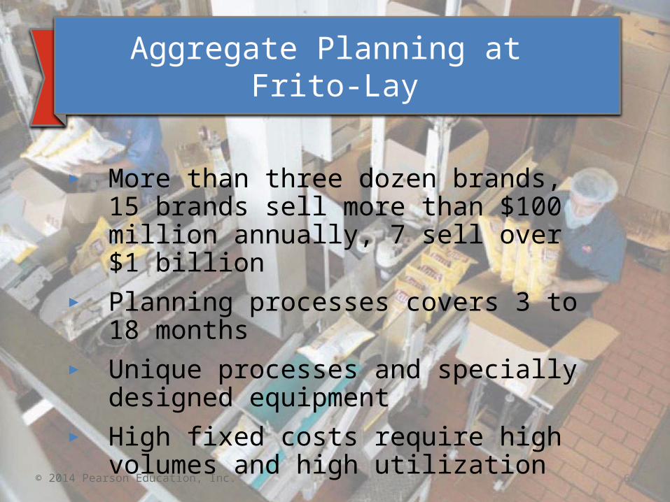
Aggregate Planning at Frito-Lay
► More than three dozen brands, 15 brands sell more than $100 million annually, 7 sell over $1 billion
► Planning processes covers 3 to 18 months► Unique processes and specially designed
equipment► High fixed costs require high volumes and high
utilization
© 2014 Pearson Education, Inc.
7
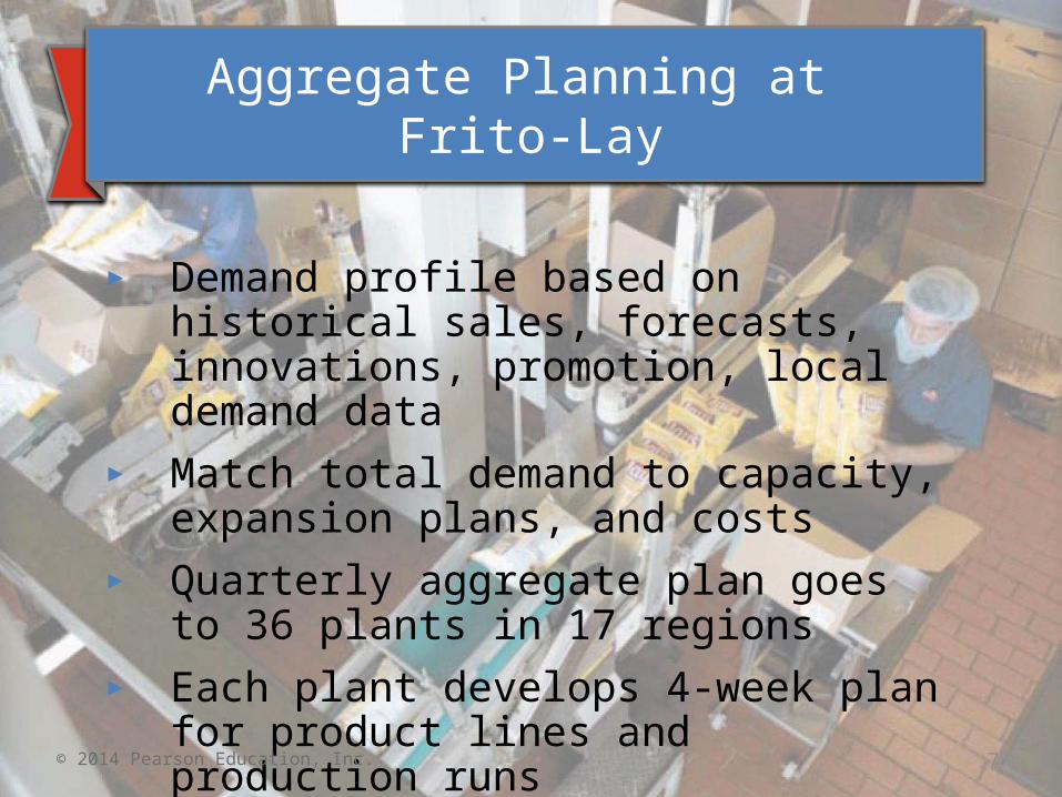
Aggregate Planning at Frito-Lay
► Demand profile based on historical sales, forecasts, innovations, promotion, local demand data
► Match total demand to capacity, expansion plans, and costs
► Quarterly aggregate plan goes to 36 plants in 17 regions
► Each plant develops 4-week plan for product lines and production runs
© 2014 Pearson Education, Inc.
8
Graphical Methods
Popular techniques Easy to understand and use Trial-and-error approaches that do not
guarantee an optimal solution Require only limited computations
9
Graphical Methods
1. Determine the demand for each period2. Determine the capacity for regular time,
overtime, and subcontracting each period3. Find labor costs, hiring and layoff costs, and
inventory holding costs4. Consider company policy on workers and stock
levels5. Develop alternative plans and examine their total
costs
10
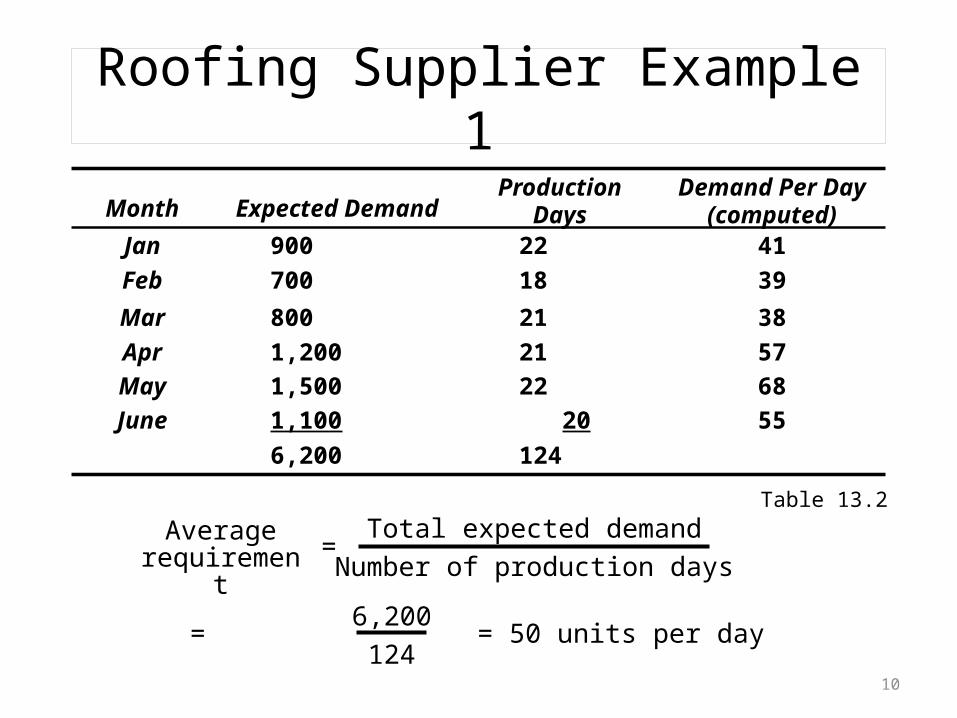
Roofing Supplier Example 1
Table 13.2
Month Expected DemandProduction
DaysDemand Per Day
(computed)
Jan 900 22 41
Feb 700 18 39
Mar 800 21 38
Apr 1,200 21 57
May 1,500 22 68
June 1,100 20 55
6,200 124
= = 50 units per day6,200124
Average requirement =
Total expected demandNumber of production days
11
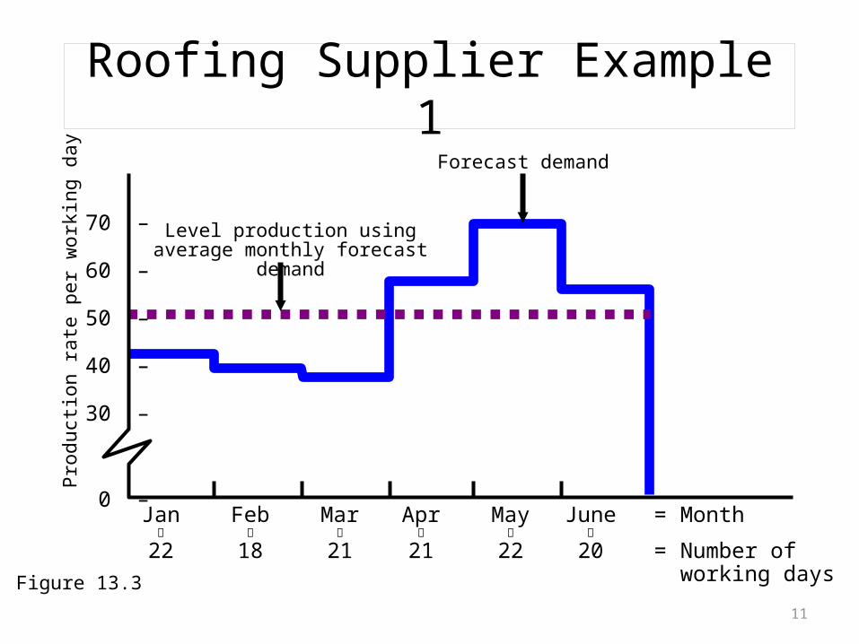
Roofing Supplier Example 1
Figure 13.3
70 –
60 –
50 –
40 –
30 –
0 –Jan Feb Mar Apr May June = Month
22 18 21 21 22 20 = Number ofworking days
Prod
uctio
n ra
te p
er w
orki
ng d
ay
Level production using average monthly forecast demand
Forecast demand
12
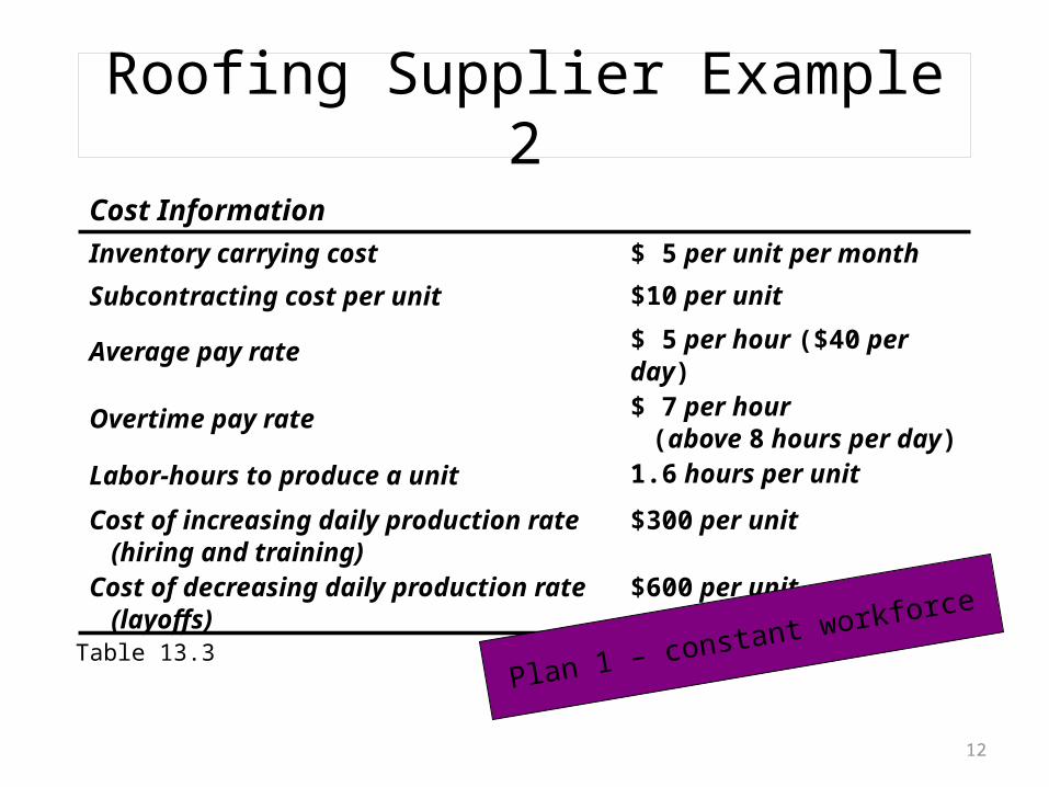
Roofing Supplier Example 2
Table 13.3
Cost Information
Inventory carrying cost $ 5 per unit per month
Subcontracting cost per unit $10 per unit
Average pay rate $ 5 per hour ($40 per day)
Overtime pay rate$ 7 per hour
(above 8 hours per day)
Labor-hours to produce a unit 1.6 hours per unit
Cost of increasing daily production rate (hiring and training)
$300 per unit
Cost of decreasing daily production rate (layoffs)
$600 per unit
Plan 1 – constant workforce
13
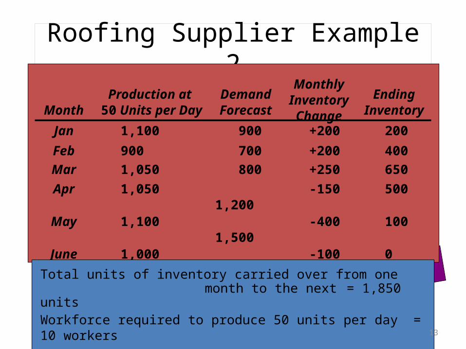
Roofing Supplier Example 2
Table 13.3
Cost Information
Inventory carry cost $ 5 per unit per month
Subcontracting cost per unit $10 per unit
Average pay rate $ 5 per hour ($40 per day)
Overtime pay rate$ 7 per hour
(above 8 hours per day)
Labor-hours to produce a unit 1.6 hours per unit
Cost of increasing daily production rate (hiring and training)
$300 per unit
Cost of decreasing daily production rate (layoffs)
$600 per unit
Plan 1 – constant workforce
MonthProduction at
50 Units per DayDemand Forecast
Monthly Inventory Change
Ending Inventory
Jan 1,100 900 +200 200Feb 900
700 +200 400
Mar 1,050800 +250 650
Apr 1,0501,200
-150 500
May 1,1001,500
-400 100
June 1,0001,100
-100
0
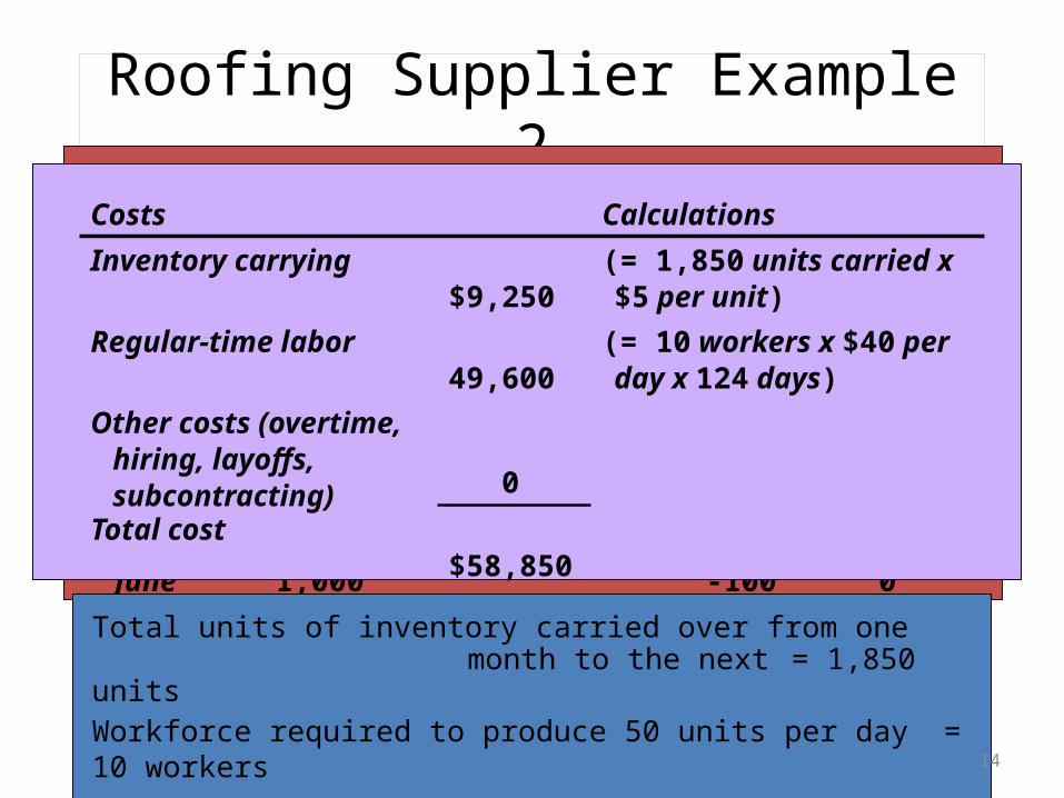
1,850
Total units of inventory carried over from onemonth to the next = 1,850 units
Workforce required to produce 50 units per day = 10 workers
14
Roofing Supplier Example 2
Table 13.3
Cost Information
Inventory carry cost $ 5 per unit per month
Subcontracting cost per unit $10 per unit
Average pay rate $ 5 per hour ($40 per day)
Overtime pay rate$ 7 per hour
(above 8 hours per day)
Labor-hours to produce a unit 1.6 hours per unit
Cost of increasing daily production rate (hiring and training)
$300 per unit
Cost of decreasing daily production rate (layoffs)
$600 per unit
MonthProduction at
50 Units per DayDemand Forecast
Monthly Inventory Change
Ending Inventory
Jan 1,100 900 +200 200Feb 900
700 +200 400
Mar 1,050800 +250 650
Apr 1,0501,200
-150 500
May 1,1001,500
-400 100
June 1,0001,100
-100
0
1,850
Total units of inventory carried over from onemonth to the next = 1,850 units
Workforce required to produce 50 units per day = 10 workers
Costs Calculations
Inventory carrying$9,250
(= 1,850 units carried x $5 per unit)
Regular-time labor49,600
(= 10 workers x $40 per day x 124 days)
Other costs (overtime, hiring, layoffs, subcontracting) 0
Total cost$58,850
15
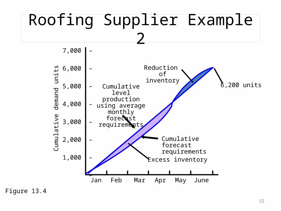
Roofing Supplier Example 2
Figure 13.4
Cum
ulati
ve d
eman
d un
its7,000 –
6,000 –
5,000 –
4,000 –
3,000 –
2,000 –
1,000 –
–Jan Feb Mar Apr May June
Cumulative forecast requirements
Cumulative level production using average monthly
forecast requirements
Reduction of inventory
Excess inventory
6,200 units
16
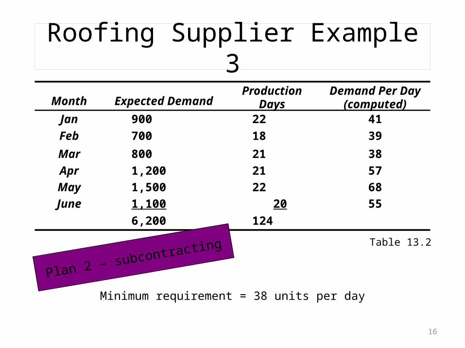
Roofing Supplier Example 3
Table 13.2
Month Expected DemandProduction
DaysDemand Per Day
(computed)
Jan 900 22 41
Feb 700 18 39
Mar 800 21 38
Apr 1,200 21 57
May 1,500 22 68
June 1,100 20 55
6,200 124
Minimum requirement = 38 units per day
Plan 2 – subcontracting
17
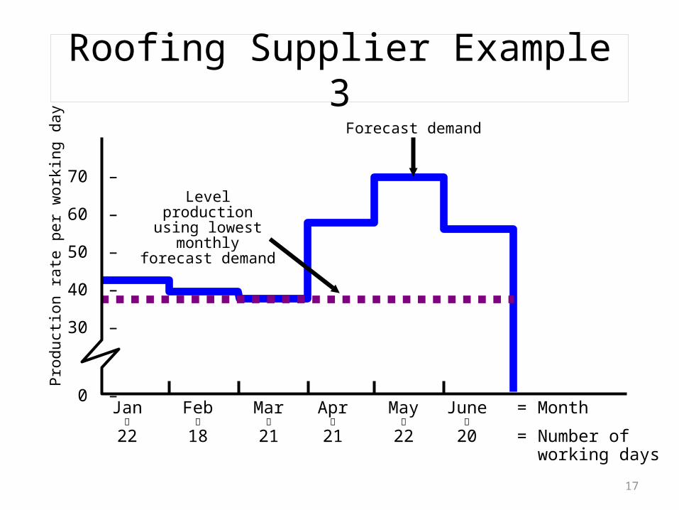
Roofing Supplier Example 3
70 –
60 –
50 –
40 –
30 –
0 –Jan Feb Mar Apr May June = Month
22 18 21 21 22 20 = Number ofworking days
Prod
uctio
n ra
te p
er w
orki
ng d
ay
Level production using lowest monthly
forecast demand
Forecast demand
18
Roofing Supplier Example 3
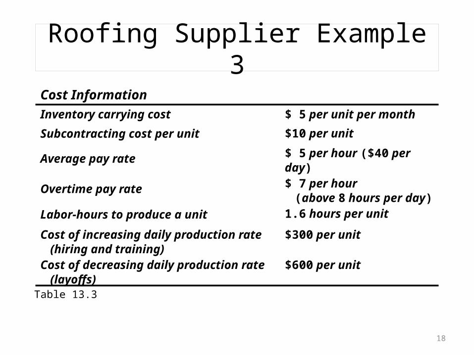
Table 13.3
Cost Information
Inventory carrying cost $ 5 per unit per month
Subcontracting cost per unit $10 per unit
Average pay rate $ 5 per hour ($40 per day)
Overtime pay rate$ 7 per hour
(above 8 hours per day)
Labor-hours to produce a unit 1.6 hours per unit
Cost of increasing daily production rate (hiring and training)
$300 per unit
Cost of decreasing daily production rate (layoffs)
$600 per unit
19
Roofing Supplier Example 3
Table 13.3
Cost Information
Inventory carry cost $ 5 per unit per month
Subcontracting cost per unit $10 per unit
Average pay rate $ 5 per hour ($40 per day)
Overtime pay rate$ 7 per hour
(above 8 hours per day)
Labor-hours to produce a unit 1.6 hours per unit
Cost of increasing daily production rate (hiring and training)
$300 per unit
Cost of decreasing daily production rate (layoffs)
$600 per unit
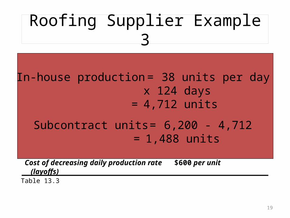
In-house production = 38 units per day x 124 days
= 4,712 units
Subcontract units = 6,200 - 4,712= 1,488 units
20
Table 13.3
Cost Information
Inventory carry cost $ 5 per unit per month
Subcontracting cost per unit $10 per unit
Average pay rate $ 5 per hour ($40 per day)
Overtime pay rate$ 7 per hour
(above 8 hours per day)
Labor-hours to produce a unit 1.6 hours per unit
Cost of increasing daily production rate (hiring and training)
$300 per unit
Cost of decreasing daily production rate (layoffs)
$600 per unit
Roofing Supplier Example 3
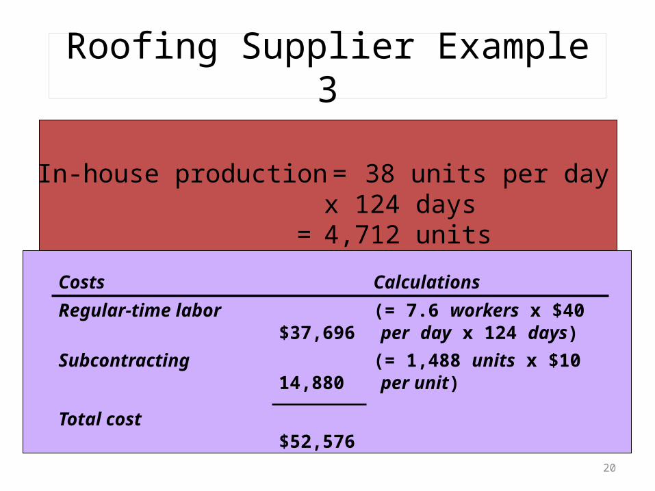
In-house production = 38 units per day x 124 days
= 4,712 units
Subcontract units = 6,200 - 4,712= 1,488 units
Costs Calculations
Regular-time labor$37,696
(= 7.6 workers x $40 per day x 124 days)
Subcontracting14,880
(= 1,488 units x $10 per unit)
Total cost$52,576
21
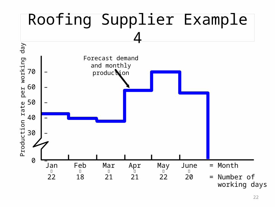
Roofing Supplier Example 4
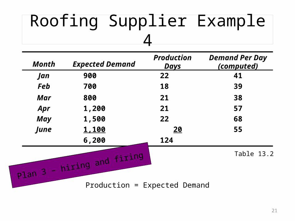
Table 13.2
Month Expected DemandProduction
DaysDemand Per Day
(computed)
Jan 900 22 41
Feb 700 18 39
Mar 800 21 38
Apr 1,200 21 57
May 1,500 22 68
June 1,100 20 55
6,200 124
Production = Expected Demand
Plan 3 – hiring and firing
22
Roofing Supplier Example 4
70 –
60 –
50 –
40 –
30 –
0 –Jan Feb Mar Apr May June = Month
22 18 21 21 22 20 = Number ofworking days
Prod
uctio
n ra
te p
er w
orki
ng d
ay
Forecast demand and monthly production

23
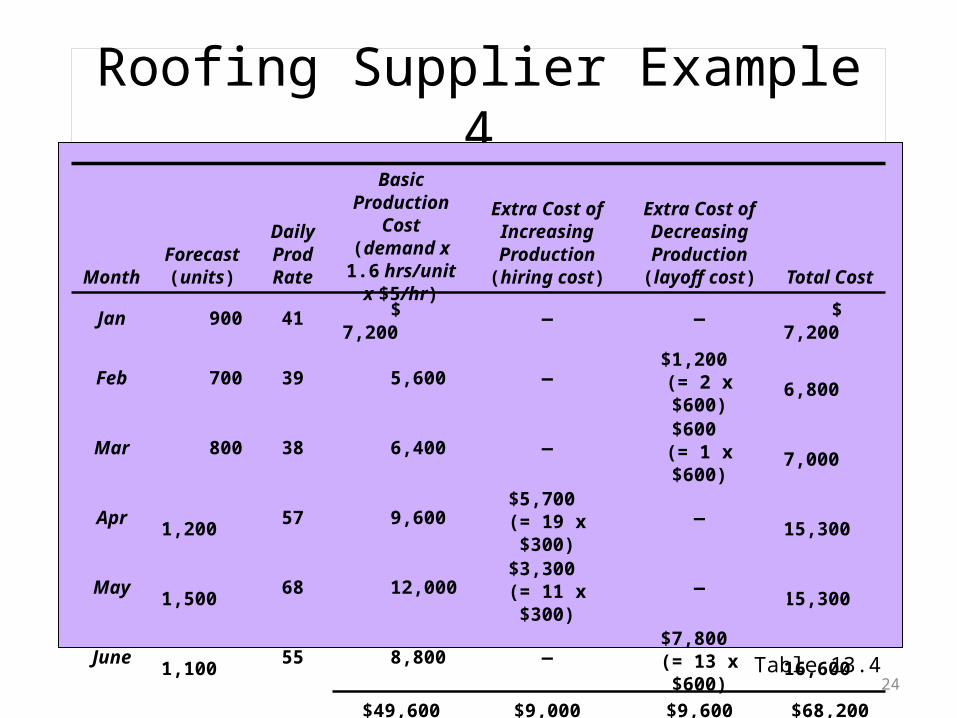
Roofing Supplier Example 4
Table 13.3
Cost Information
Inventory carrying cost $ 5 per unit per month
Subcontracting cost per unit $10 per unit
Average pay rate $ 5 per hour ($40 per day)
Overtime pay rate$ 7 per hour
(above 8 hours per day)
Labor-hours to produce a unit 1.6 hours per unit
Cost of increasing daily production rate (hiring and training)
$300 per unit
Cost of decreasing daily production rate (layoffs)
$600 per unit
24
Roofing Supplier Example 4
Table 13.3
Cost Information
Inventory carrying cost $ 5 per unit per month
Subcontracting cost per unit $10 per unit
Average pay rate $ 5 per hour ($40 per day)
Overtime pay rate$ 7 per hour
(above 8 hours per day)
Labor-hours to produce a unit 1.6 hours per unit
Cost of increasing daily production rate (hiring and training)
$300 per unit
Cost of decreasing daily production rate (layoffs)
$600 per unit
MonthForecast
(units)
Daily Prod Rate
Basic Production
Cost (demand x
1.6 hrs/unit x $5/hr)
Extra Cost of Increasing Production (hiring cost)
Extra Cost of Decreasing Production (layoff cost) Total Cost
Jan 900 41 $ 7,200 — — $ 7,200
Feb 700 39 5,600 — $1,200 (= 2 x $600) 6,800
Mar 800 38 6,400 — $600 (= 1 x $600) 7,000
Apr 1,200 57 9,600$5,700
(= 19 x $300) — 15,300
May 1,500 68 12,000$3,300
(= 11 x $300) — 15,300
June 1,100 55 8,800 — $7,800 (= 13 x $600) 16,600
$49,600 $9,000 $9,600 $68,200
Table 13.4
25
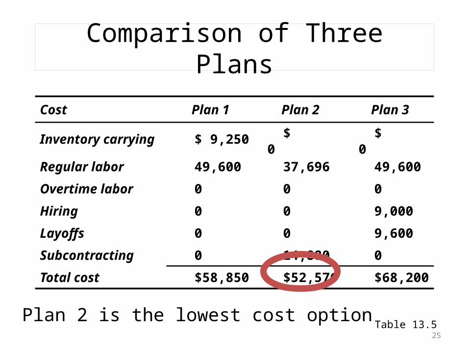
Comparison of Three Plans
Table 13.5
Cost Plan 1 Plan 2 Plan 3
Inventory carrying $ 9,250
$ 0
$ 0
Regular labor 49,600 37,696 49,600
Overtime labor 0 0 0
Hiring 0 0 9,000
Layoffs 0 0 9,600
Subcontracting 0 14,880 0
Total cost $58,850 $52,576 $68,200Plan 2 is the lowest cost option
26
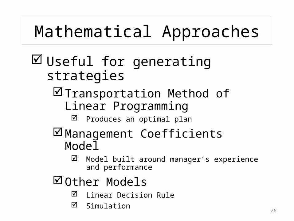
Mathematical Approaches
Useful for generating strategiesTransportation Method of Linear
Programming Produces an optimal plan
Management Coefficients Model Model built around manager’s experience and
performance
Other Models Linear Decision Rule Simulation
27
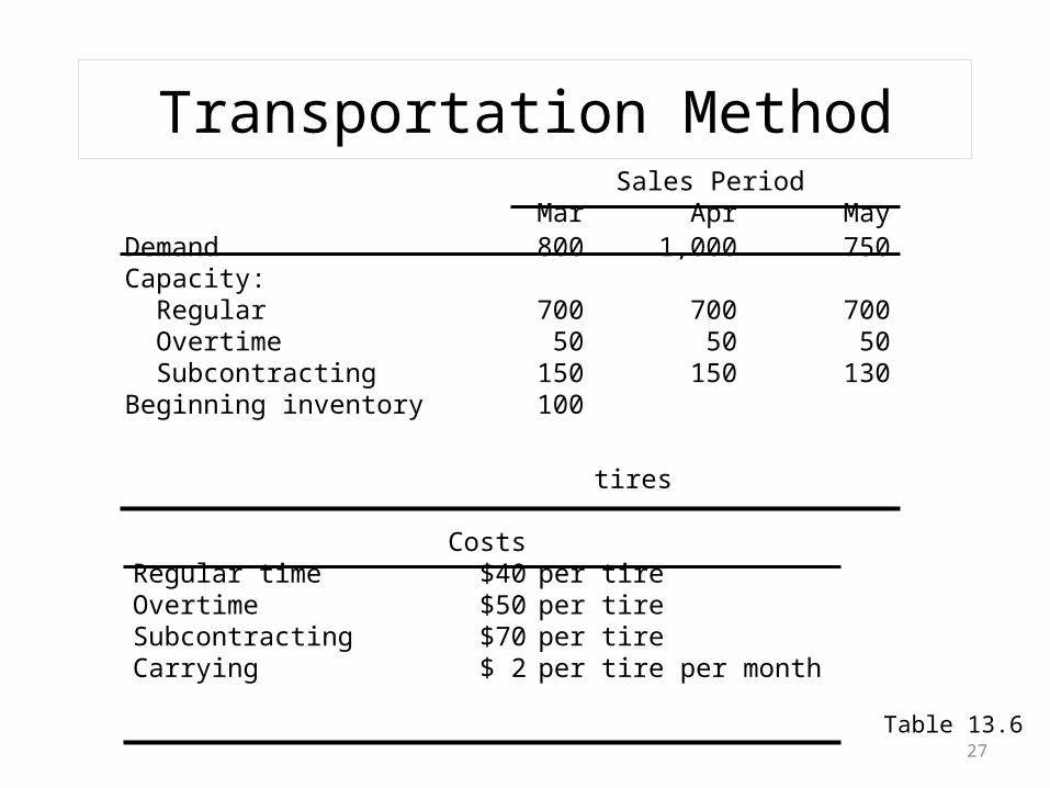
Transportation Method
Table 13.6
CostsRegular time $40 per tireOvertime $50 per tireSubcontracting $70 per tireCarrying $ 2 per tire per month
Sales PeriodMar Apr May
Demand 800 1,000 750Capacity: Regular 700 700 700 Overtime 50 50 50 Subcontracting 150 150 130Beginning inventory 100
tires
28
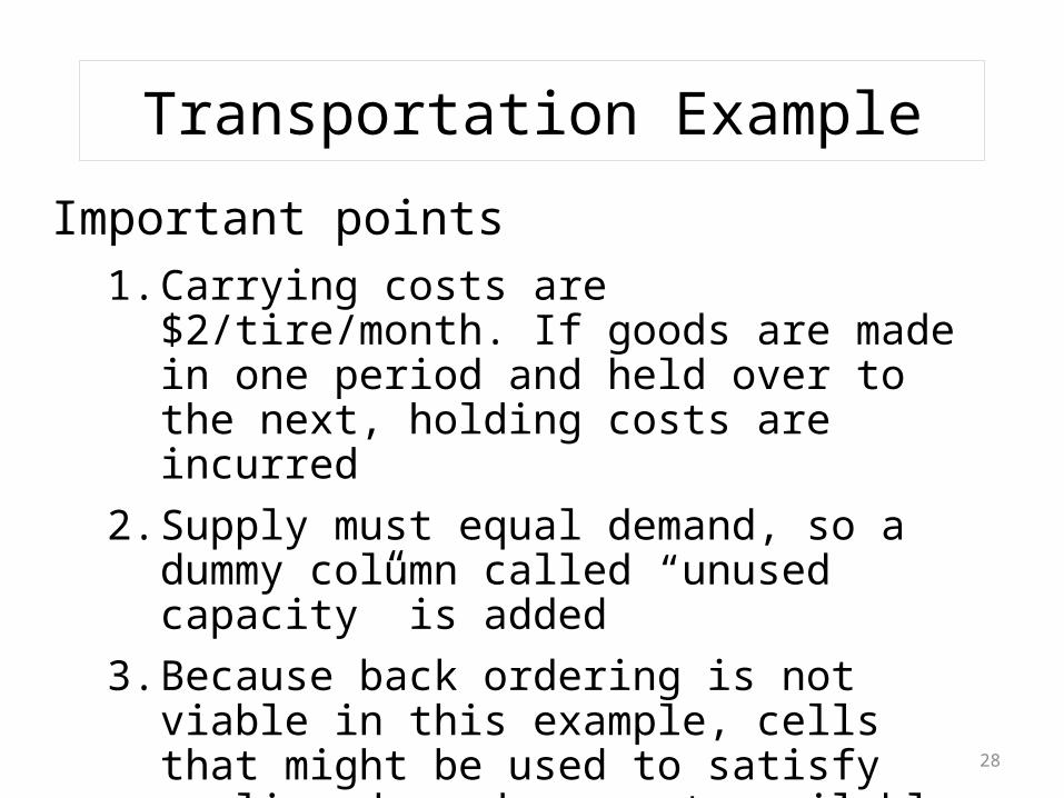
Transportation Example
Important points1. Carrying costs are $2/tire/month. If goods are
made in one period and held over to the next, holding costs are incurred
2. Supply must equal demand, so a dummy column called “unused capacity” is added
3. Because back ordering is not viable in this example, cells that might be used to satisfy earlier demand are not available
29
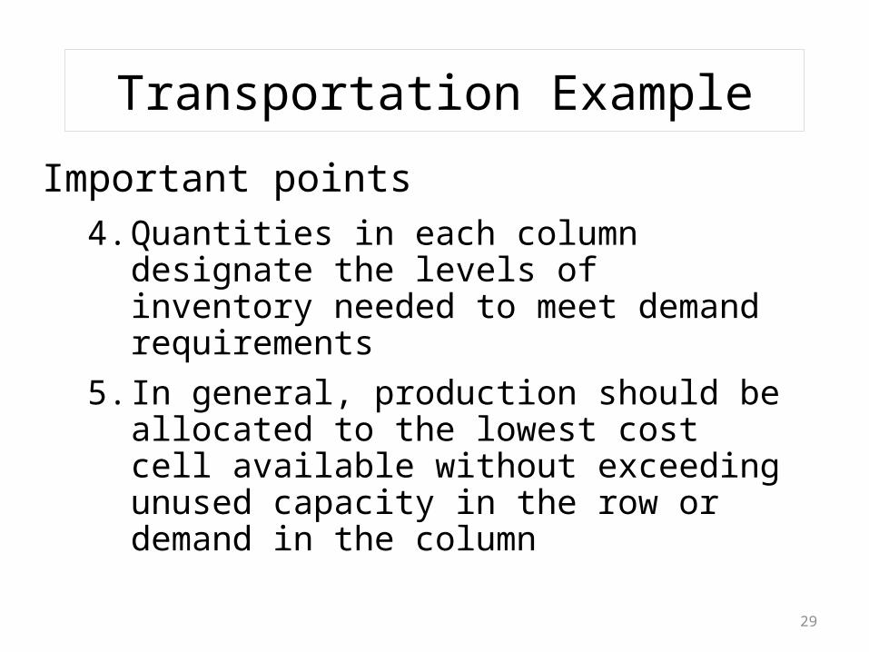
Transportation Example
Important points4. Quantities in each column designate the levels
of inventory needed to meet demand requirements
5. In general, production should be allocated to the lowest cost cell available without exceeding unused capacity in the row or demand in the column
30
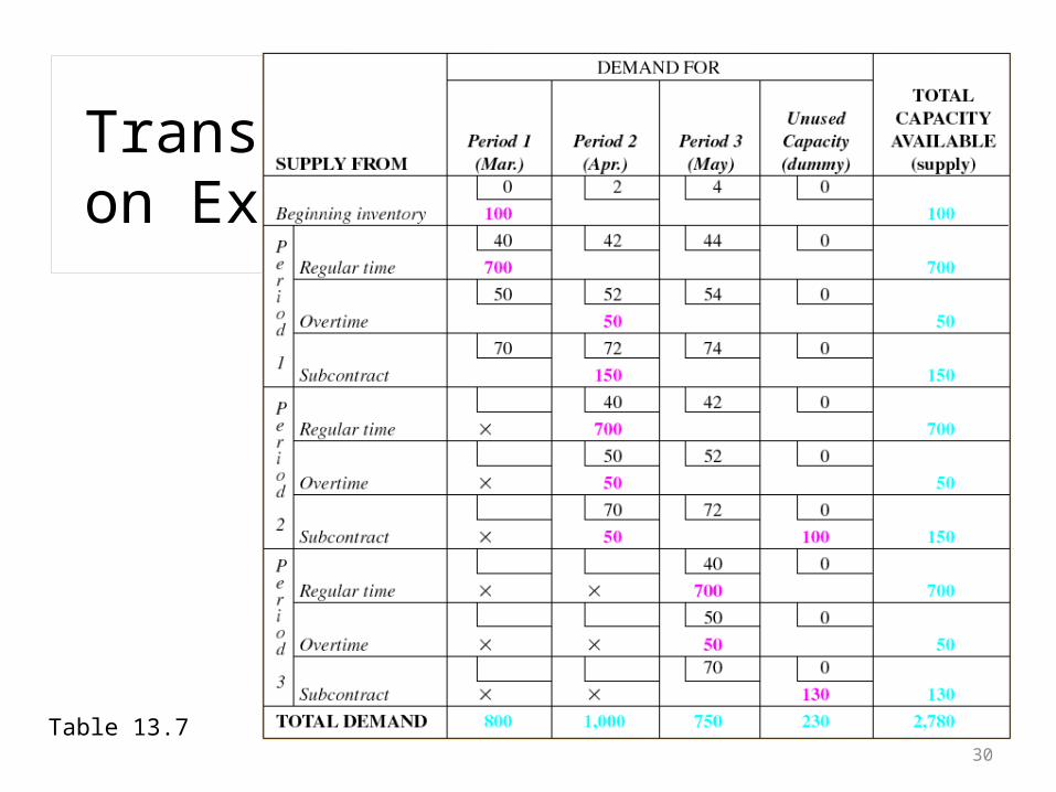
Transportation Example
Table 13.7
31
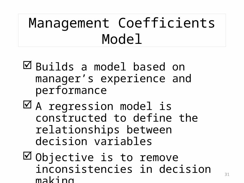
Management Coefficients Model
Builds a model based on manager’s experience and performance
A regression model is constructed to define the relationships between decision variables
Objective is to remove inconsistencies in decision making
32
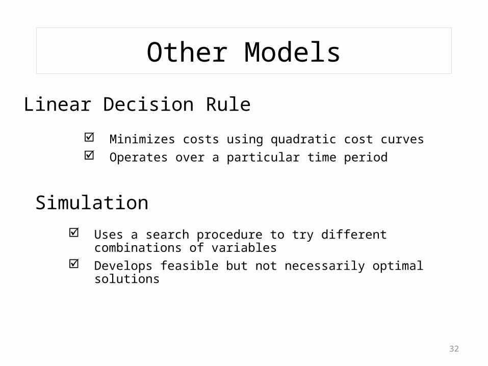
Other Models
Linear Decision Rule
Minimizes costs using quadratic cost curves Operates over a particular time period
Simulation Uses a search procedure to try different combinations of variables Develops feasible but not necessarily optimal solutions
33
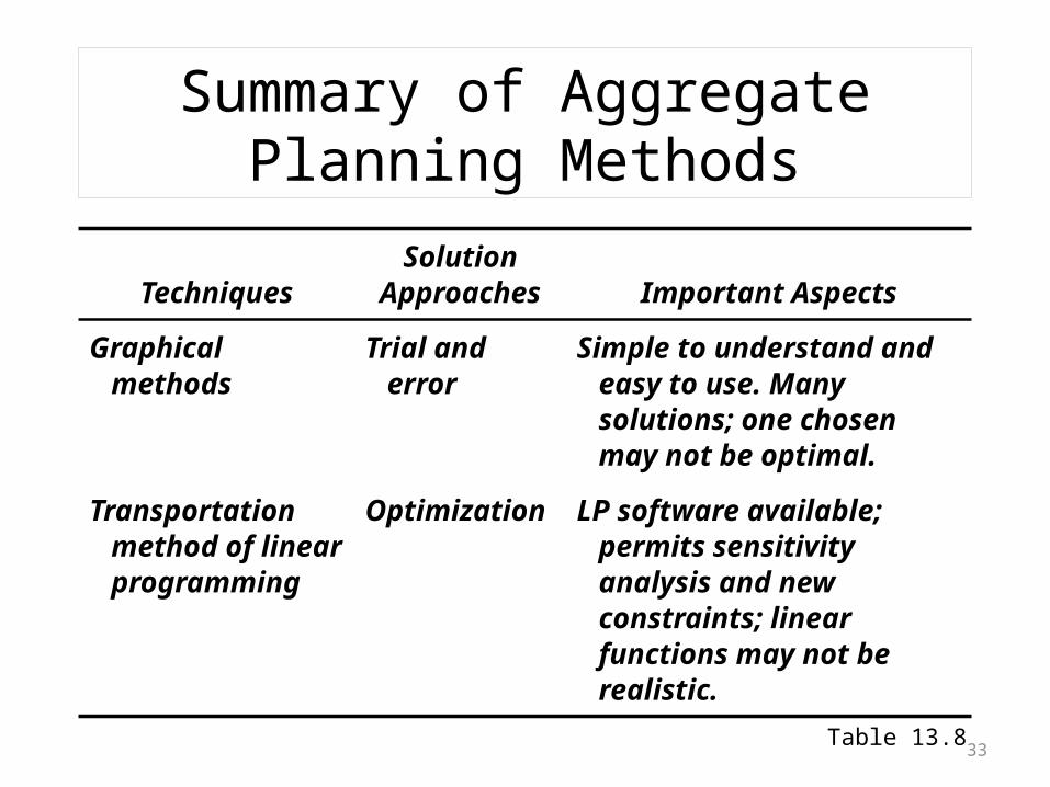
Summary of Aggregate Planning Methods
TechniquesSolution
Approaches Important Aspects
Graphicalmethods
Trial and error
Simple to understand and easy to use. Many solutions; one chosen may not be optimal.
Transportation method of linear programming
Optimization LP software available; permits sensitivity analysis and new constraints; linear functions may not be realistic.
Table 13.8
34
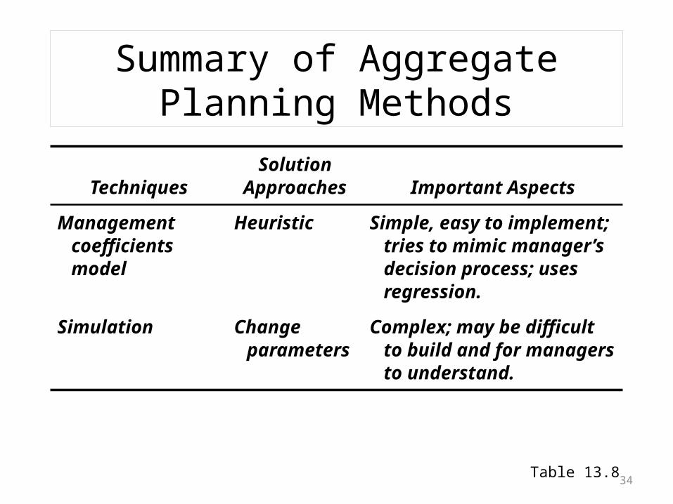
Summary of Aggregate Planning Methods
TechniquesSolution
Approaches Important Aspects
Management coefficients model
Heuristic Simple, easy to implement; tries to mimic manager’s decision process; uses regression.
Simulation Change parameters
Complex; may be difficult to build and for managers to understand.
Table 13.8
35
Aggregate Planning in Services
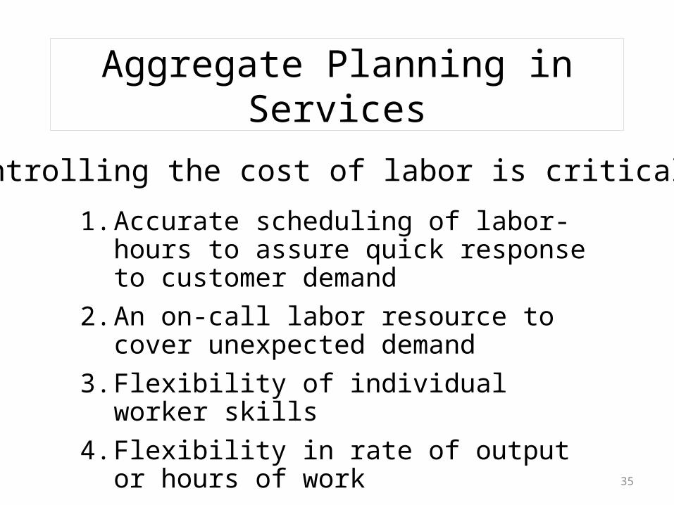
Controlling the cost of labor is critical
1. Accurate scheduling of labor-hours to assure quick response to customer demand
2. An on-call labor resource to cover unexpected demand
3. Flexibility of individual worker skills4. Flexibility in rate of output or hours of work

36
Five Service Scenarios
Restaurants Smoothing the production processDetermining the optimal workforce size
HospitalsResponding to patient demand
37
Five Service Scenarios
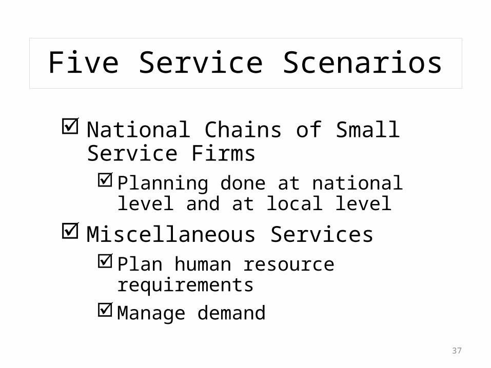
National Chains of Small Service FirmsPlanning done at national level and at
local level Miscellaneous Services
Plan human resource requirementsManage demand
38
Law Firm Example
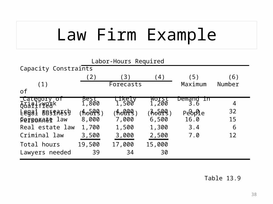
Table 13.9
Labor-Hours Required Capacity Constraints(2) (3) (4) (5) (6)
(1) Forecasts Maximum Number ofCategory of Best Likely Worst Demand in Qualified
Legal Business (hours) (hours) (hours) People Personnel
Trial work 1,800 1,500 1,200 3.6 4Legal research 4,500 4,000 3,500 9.0 32Corporate law 8,000 7,000 6,500 16.0 15Real estate law 1,700 1,500 1,300 3.4 6Criminal law 3,500 3,000 2,500 7.0 12Total hours 19,500 17,000 15,000Lawyers needed 39 34 30
39
Five Service Scenarios
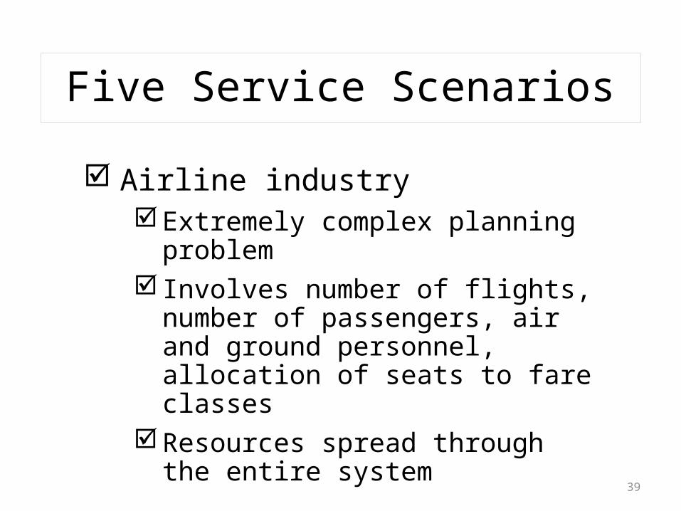
Airline industryExtremely complex planning problem Involves number of flights, number of
passengers, air and ground personnel, allocation of seats to fare classes
Resources spread through the entire system
40
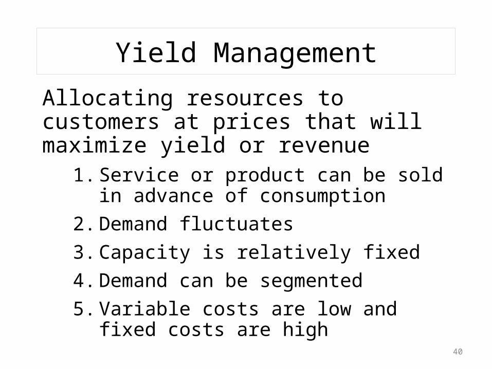
Yield Management
Allocating resources to customers at prices that will maximize yield or revenue
1. Service or product can be sold in advance of consumption
2. Demand fluctuates3. Capacity is relatively fixed4. Demand can be segmented5. Variable costs are low and fixed costs are
high
41
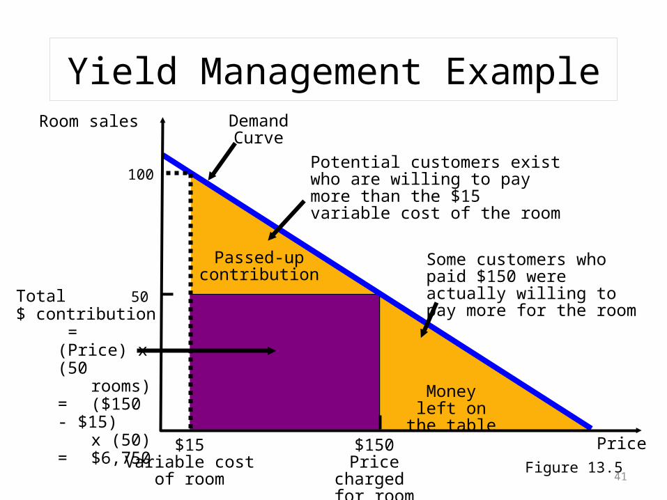
Demand Curve
Yield Management Example
Figure 13.5
Passed-up contribution
Money left on the table
Potential customers exist who are willing to pay more than the $15 variable cost of the room
Some customers who paid $150 were actually willing to pay more for the roomTotal
$ contribution =(Price) x (50
rooms)=($150 - $15)
x (50)=$6,750
Price
Room sales
100
50
$150Price charged
for room
$15Variable cost
of room
42
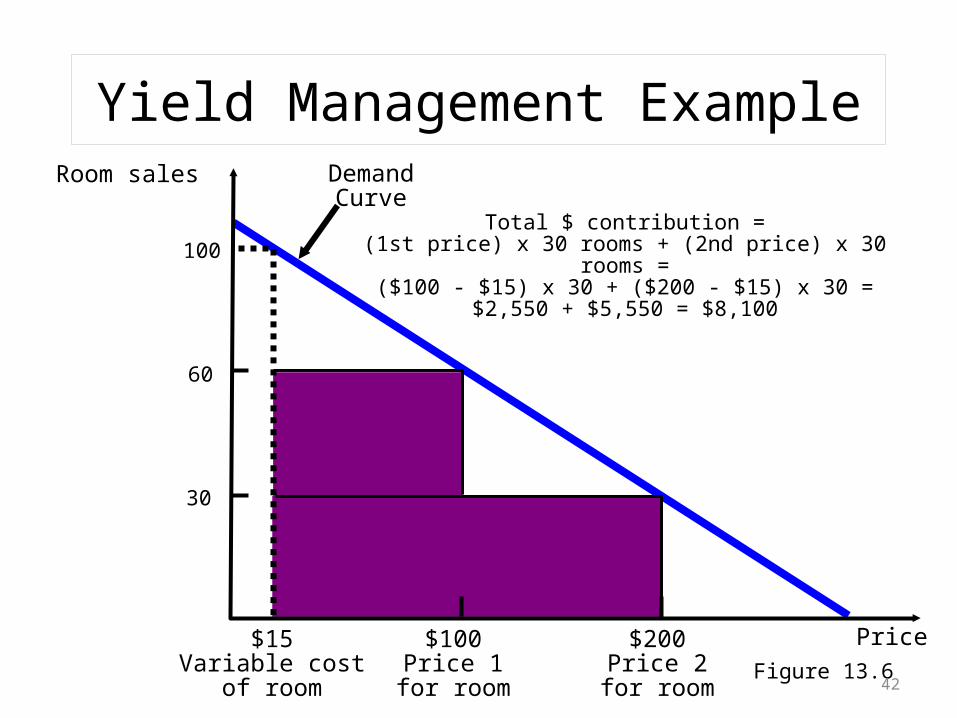
Total $ contribution =(1st price) x 30 rooms + (2nd price) x 30 rooms =
($100 - $15) x 30 + ($200 - $15) x 30 =$2,550 + $5,550 = $8,100
Demand Curve
Yield Management Example
Figure 13.6
Price
Room sales
100
60
30
$100Price 1
for room
$200Price 2
for room
$15Variable cost
of room
43
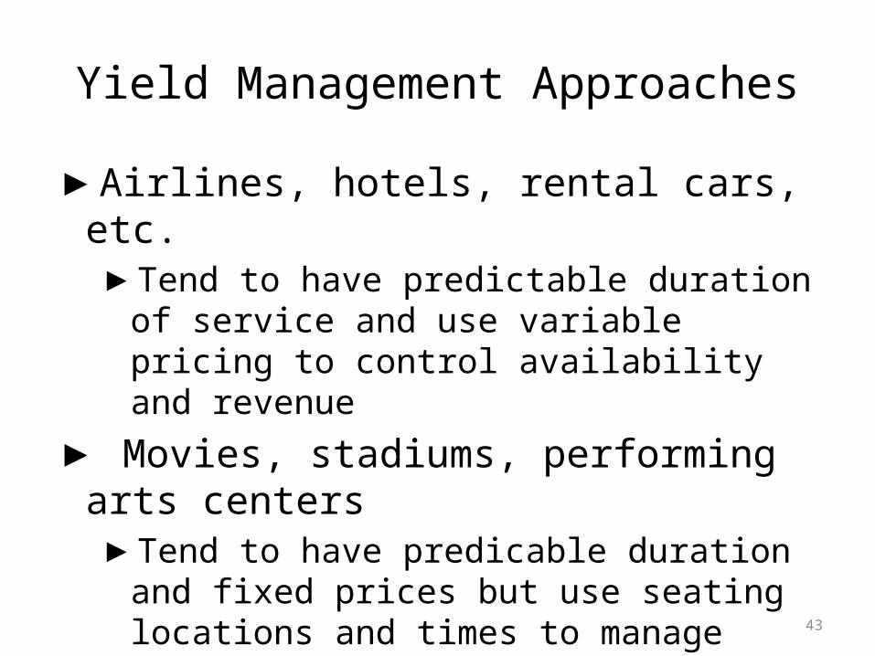
Yield Management Approaches
▶Airlines, hotels, rental cars, etc.▶ Tend to have predictable duration of service
and use variable pricing to control availability and revenue
▶ Movies, stadiums, performing arts centers▶ Tend to have predicable duration and fixed
prices but use seating locations and times to manage revenue
44
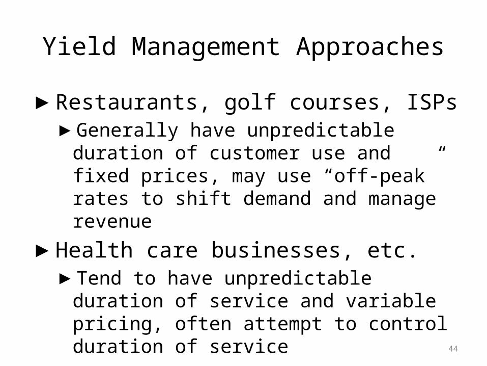
Yield Management Approaches
▶Restaurants, golf courses, ISPs▶ Generally have unpredictable duration of
customer use and fixed prices, may use “off-peak” rates to shift demand and manage revenue
▶Health care businesses, etc.▶ Tend to have unpredictable duration of
service and variable pricing, often attempt to control duration of service
45
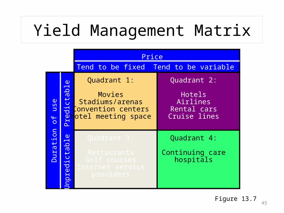
Yield Management MatrixD
urati
on o
f use
Unp
redi
ctab
le
Pred
icta
ble
PriceTend to be fixed Tend to be variable
Quadrant 1: Quadrant 2:
Movies HotelsStadiums/arenas Airlines
Convention centers Rental carsHotel meeting space Cruise lines
Quadrant 3: Quadrant 4:
Restaurants Continuing careGolf courses hospitals
Internet serviceproviders
Figure 13.7
46
Making Yield Management Work
1. Multiple pricing structures must be feasible and appear logical to the customer
2. Forecasts of the use and duration of use
3. Changes in demand

47
Summary of this Session
Case Study Frito Lays for Aggregate Planning
Graphical MethodsMathematical ApproachesComparison of Aggregate Planning
Methods
48
Summary of this Session (Contd.) Aggregate Planning in Services
RestaurantsHospitalsNational Chains of Small Service FirmsMiscellaneous Services
Airline Industry Yield Management

49
THANK YOU