lto noise prediction methodology for sst aircraft
TRANSCRIPT

Politecnico di Torino
DEPARTMENT OF MECHANICAL AND AEROSPACE ENGINEERING
Master of Science programme Aerospace engineeringGraduation session July 2021
LTO noise prediction methodologyfor SST aircraft conceptual design
Thesis advisor:
Prof. Nicole Viola
Research supervisors:
Ing. Luigi FedericoProf. Roberta Fusaro
Candidate:
Grazia Piccirillo
ID number s265939
Academic year 2020/2021


Alla mia famiglia, peraver sempre creduto inme.A Lorenzo, per esserestato costantemente almio fianco.
Abstract
The new emerging generation of SuperSonic Transport (SST) aircraft demandsan enhanced approach for the consideration and analysis of its impact on environ-ment, with the subsequent delivery of relevant Standards and Recommended Practices(SARPs) to make the certification of a supersonic aeroplane possible in the 2020-2025timeframe. Focusing on noise generated during Landing and Take-Off (LTO) cycle,the presented activities address the development of a methodology aimig at predictingnoise levels in the early stages of SST aircraft design process, accounting for noiserequirements as a design constraint and supporting a design-to-noise approach. Themethodology includes a supersonic aircraft noise model in which overall aircraft noiseis predicted as an assembly of major noise sources, each modelled with an individ-ual semi-empirical noise source model based on the equations reported in “AircraftNoise Prediction Program – Theoretical Manual” published by NASA. Following theaeroacoustics modelling applied in Aircraft NOise Prediction Program (ANOPP), themajor LTO noise sources of an SST aircraft have been selected and in addition thenoise attenuation due to the propagation in the atmosphere has been considered inaccordance with SAE ARP 866 B. The integration of the noise model within the over-all methodology framework leads to the prediction of the aircraft noise level. Theaccuracy of the method in predicting the overall aircraft noise level has been esti-mated through a dedicated validation with experimental data provided by the AircraftNoise and Performance (ANP) database for flyover trajectories at different altitudesand thrust ratings. Considering that the goal of the methodology is to predict noiselevels for future supersonic aircraft, the only available supersonic aircraft of the ANP,i.e. the Concorde, has been selected as case study. The matching with Noise PowerDistance (NPD) curves has been evaluated for maximum A-weighting sound pressurelevel (LAmax) and Sound Exposure Level (SEL). Ranging from an altitude of about200 m to 3000 m, the results have showed that the prediction error falls within ±1.5dBA. Considering that the accuracy is acceptable for applications at a conceptual de-sign level, the overall methodology has been applied to predict noise level at the threecertification measuring points (sideline, flyover and approach) defined by ICAO. Theresults have been reported for each noise source contribution and overall aircraft noise,identifying jet noise as the dominant LTO noise source. The outcome of this researchactivity demonstrates the capability of the developed methodology in introducing noiseevaluations since the early stages of aircraft design. With appropriate improvementsin noise source and engine modelling, the methodology can be useful to provide guide-lines for the design of future low-noise SST together with operational procedures ableto mitigate the LTO noise.

Ringraziamenti
Giunta al termine di questo percorso, desidero innanzitutto ringraziare la professores-sa Nicole Viola e la professoressa Roberta Fusaro, per avermi offerto l’opportunità diaffrontare tematiche innovative all’interno della tesi e per avermi accompagnato co-stantemente e con estrema disponibilità in questo sfidante lavoro, incoraggiorandomie fornendomi tutto il supporto necessario, nonostante le difficoltà del periodo storicoche stiamo vivendo. Un ringraziamento speciale va all’Ing. Luigi Federico, ricercatorepresso il Centro Italiano Ricerche Aerospaziali (CIRA), per aver riposto grande fidu-cia in me e aver messo a mia disposizione le sue elevate competenze, supervisionandooperosamente le diverse attività svolte. Sono sinceramente onorata di aver collaboratocon Voi e farò certamente tesoro di tutto ciò che mi avete dato modo di apprendere perla mia futura carriera. Dal punto di vista personale, mi è doveroso ringraziare la miafamiglia: mio padre, mia madre, mio fratello e mia Zia Assunta. Sono infinitamentegrata a loro per avermi concesso di vivere questo grande sogno e per aver preso parte adogni mio successo o delusione, riuscendo sempre pienamente a comprendermi e soste-nermi, nonostante le peculiarità dei miei studi. Ringrazio poi, tutti i miei colleghi, tracui vecchie e nuove amicizie. Vi ringrazio per tutto ciò che, forse inconsapevolmente,mi avete insegnato, ma anche per l’empatia, il conforto e i sorrisi condivisi insieme eche, anche a chilometri di distanza da casa, non mi hanno fatto mai sentire sola. Nonposso fare a meno di ringraziare le mie amiche di sempre, Fefi e Nancy, che rappresen-tano per me il sostegno più prezioso. Grazie per aver sempre creduto in me, per esserestate sempre presenti con piccoli e grandi gesti, per avermi capita e essermi venuteincontro, nonostante le nostre diversità, la distanza e gli impegni. Ancora, ringraziola mia coinquilina Martina, la mia vera complice durante tutta questa esperienza e lascoperta più sensazionale che potessi fare. Non basterebbero tutte le pagine di questatesi per elencare i motivi per cui debba ringraziarti; abbiamo riso, abbiamo pianto,abbiamo vissuto mille emozioni insieme e ti ringrazio per essere stata sempre al miofianco, proprio come farebbe una sorella. Last but not least, ringrazio il mio fidanzatoLorenzo e la sua famiglia, per avermi sempre sostenuta e incoraggiata, facendo dissol-vere le mie ansie e dandomi sicurezza. In particolare, ringrazio Lorenzo, per quellalungimiranza di cui mi sono fidata e che mi ha dato il coraggio di uscire dalla miacomfort zone e provare sempre più a superare i miei limiti: se oggi sono una personamigliore è soprattutto grazie a te.
2

Contents
List of Tables 5
List of Figures 6
1 Introduction 91.1 The environmental concern . . . . . . . . . . . . . . . . . . . . . . . . . 91.2 Sustainable supersonic flight . . . . . . . . . . . . . . . . . . . . . . . . 11
1.2.1 Noise acceptability and regulation . . . . . . . . . . . . . . . . . 141.3 Research goal . . . . . . . . . . . . . . . . . . . . . . . . . . . . . . . . 19
2 Noise source modelling 212.1 Literature review . . . . . . . . . . . . . . . . . . . . . . . . . . . . . . 21
2.1.1 ANOPP . . . . . . . . . . . . . . . . . . . . . . . . . . . . . . . 242.2 SST aircraft LTO noise model . . . . . . . . . . . . . . . . . . . . . . . 26
2.2.1 Airframe noise . . . . . . . . . . . . . . . . . . . . . . . . . . . . 282.2.2 Engine noise . . . . . . . . . . . . . . . . . . . . . . . . . . . . . 332.2.3 Output . . . . . . . . . . . . . . . . . . . . . . . . . . . . . . . . 42
3 Overall methodology 513.1 Framework . . . . . . . . . . . . . . . . . . . . . . . . . . . . . . . . . . 513.2 Engine model . . . . . . . . . . . . . . . . . . . . . . . . . . . . . . . . 543.3 Trajectory simulation . . . . . . . . . . . . . . . . . . . . . . . . . . . . 613.4 Noise metrics . . . . . . . . . . . . . . . . . . . . . . . . . . . . . . . . 62
4 Validation 694.1 Case study . . . . . . . . . . . . . . . . . . . . . . . . . . . . . . . . . . 694.2 ANP database . . . . . . . . . . . . . . . . . . . . . . . . . . . . . . . . 754.3 Results . . . . . . . . . . . . . . . . . . . . . . . . . . . . . . . . . . . . 76
5 Application 855.1 Departure . . . . . . . . . . . . . . . . . . . . . . . . . . . . . . . . . . 855.2 Approach . . . . . . . . . . . . . . . . . . . . . . . . . . . . . . . . . . 89
6 Conclusions and further developments 91
3

A Main noise sources 93
B Airframe noise directivity 95
C Engine noise directivity 97
Bibliography 99
4

List of Tables
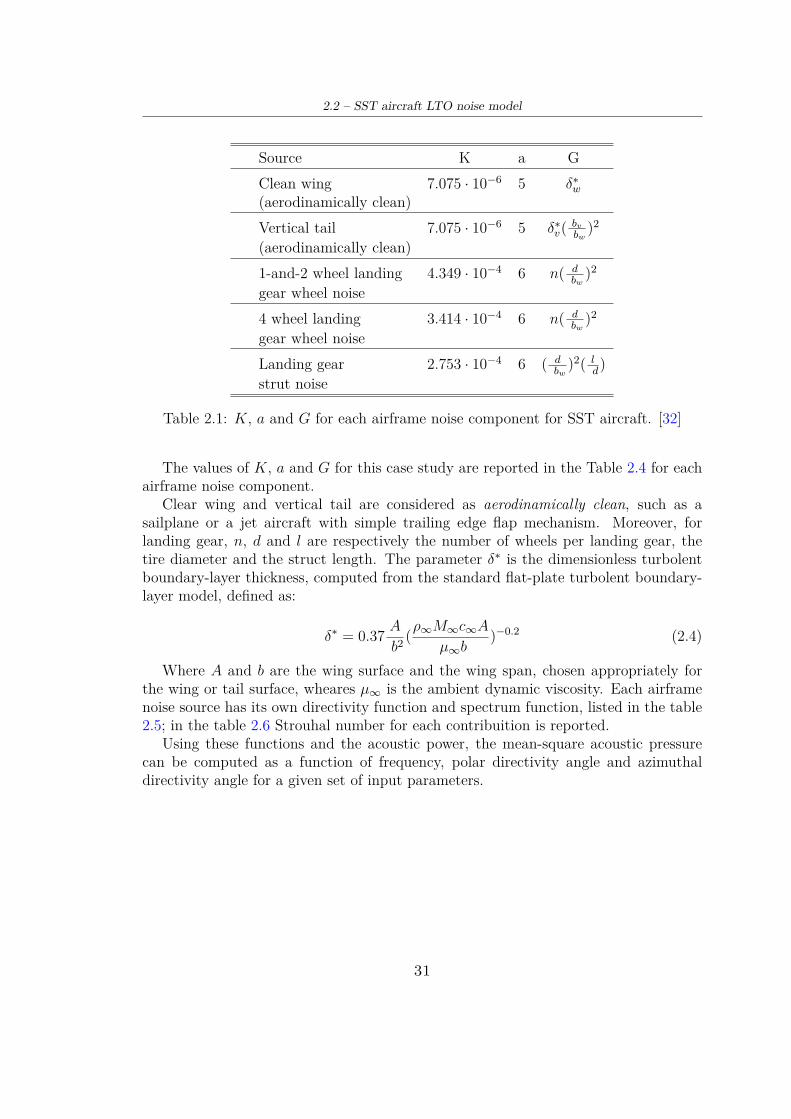
2.1 K, a and G for each airframe noise component for SST aircraft. [32] . . 312.2 Directivity function D and Spectrum function F (S) for each airframe
noise component for SST aircraft [32] . . . . . . . . . . . . . . . . . . . 322.3 Strouhal number S for each airframe noise component for SST aircraft
[32] . . . . . . . . . . . . . . . . . . . . . . . . . . . . . . . . . . . . . . 322.4 Flight path and ambient conditions data. . . . . . . . . . . . . . . . . . 422.5 Airframe noise parameters for noise prediction. . . . . . . . . . . . . . . 432.6 Jet noise parameters for noise prediction. . . . . . . . . . . . . . . . . . 442.7 Fan noise parameters for noise prediction. . . . . . . . . . . . . . . . . 463.1 On design condition - parameters definition. [41] . . . . . . . . . . . . . 574.1 Concorde reference airframe data . . . . . . . . . . . . . . . . . . . . . 724.2 Concorde reference engine data . . . . . . . . . . . . . . . . . . . . . . 734.3 Concorde reference weights and loadings . . . . . . . . . . . . . . . . . 734.4 Concorde reference performance . . . . . . . . . . . . . . . . . . . . . . 744.5 Concorde reference operational noise characteristics . . . . . . . . . . . 744.6 Aircraft speed and ambient conditions. . . . . . . . . . . . . . . . . . . 774.7 Altitude variations. . . . . . . . . . . . . . . . . . . . . . . . . . . . . . 774.8 Thrust variations. . . . . . . . . . . . . . . . . . . . . . . . . . . . . . . 774.9 Prediction error - LAmax and SEL. . . . . . . . . . . . . . . . . . . . . 804.10 RMSE - LAmax and SEL. . . . . . . . . . . . . . . . . . . . . . . . . . 815.1 Fixed point data for departure procedure. . . . . . . . . . . . . . . . . 865.2 Noise levels for each contribution and overall aircraft noise - Sideline . . 875.3 Noise levels for each contribution and overall aircraft noise - Flyover . . 885.4 Fixed point data for approach procedure. . . . . . . . . . . . . . . . . . 895.5 Noise levels for each contribution and overall aircraft noise - Approach 90A.1 Overview of airframe noise sources [33] . . . . . . . . . . . . . . . . . . 93A.2 Overview of engine noise sources [33] . . . . . . . . . . . . . . . . . . . 94
5

List of Figures
1.1 Global RPKs per years.[1] . . . . . . . . . . . . . . . . . . . . . . . . . 101.2 Replacement as a share of new deliveries. [2] . . . . . . . . . . . . . . . 101.3 CAEP deliverables. [4] . . . . . . . . . . . . . . . . . . . . . . . . . . . 111.4 Low-boom flight demonstrator X-59 QueSST. . . . . . . . . . . . . . . 131.5 Future supersonic airliner Overture. . . . . . . . . . . . . . . . . . . . . 131.6 Future supersonic business jet Spike S-512. . . . . . . . . . . . . . . . . 141.7 Jet aircraft noise levels at entry into service until 1990. [11] . . . . . . . 151.8 The progression of the ICAO LTO noise Standards for aeroplanes –
Cumulative noise limits vs. Maximum Take-Off Mass (MTOM). [13] . . 161.9 Aircraft noise certification reference measurement points. [20] . . . . . 171.10 Sonic boom pressure far-field wave patterns.[15] . . . . . . . . . . . . . 181.11 Roadmap of the activities performed in the thesis. . . . . . . . . . . . . 202.1 Aircraft noise prediction problem [23]. . . . . . . . . . . . . . . . . . . 252.2 Flow chart of ANOPP functional modules.[24]. . . . . . . . . . . . . . . 262.3 SST aircraft LTO noise sources breakdown. . . . . . . . . . . . . . . . . 282.4 Individual noise-radiating airframe components.[35] . . . . . . . . . . . 292.5 Summary of engine noise sources (General Electric Affinity by GE Avi-
ation - Turbofan for supersonic transport) . . . . . . . . . . . . . . . . 332.6 Jet flow exhaust mixing and shock structure. . . . . . . . . . . . . . . . 342.7 Fan inlet and discharge noise. . . . . . . . . . . . . . . . . . . . . . . . 382.8 Airframe noise SPL (θ = 90◦,φ = 0◦). . . . . . . . . . . . . . . . . . . . 432.9 Jet noise SPL (θ = 90◦,φ = 0◦). . . . . . . . . . . . . . . . . . . . . . . 442.10 Jet mixing noise SPL versus Vj . . . . . . . . . . . . . . . . . . . . . . . 452.11 Shock cells noise SPL versus Mj . . . . . . . . . . . . . . . . . . . . . . 452.12 Fan noise SPL (θ = 90◦,φ = 0◦). . . . . . . . . . . . . . . . . . . . . . . 472.13 Fan noise SPL versus m. . . . . . . . . . . . . . . . . . . . . . . . . . . 482.14 Fan noise SPL versus N . . . . . . . . . . . . . . . . . . . . . . . . . . . 482.15 Fan noise SPL versus ∆T . . . . . . . . . . . . . . . . . . . . . . . . . . 482.16 Overall aircraft noise SPL - subsonic and supersonic jet. . . . . . . . . 493.1 Overall methodology framework. . . . . . . . . . . . . . . . . . . . . . . 533.2 Coordinate reference system. . . . . . . . . . . . . . . . . . . . . . . . . 543.3 Rolls Royce Olympus 593 MRK 610. . . . . . . . . . . . . . . . . . . . 553.4 Engine station designation for a two-spool turbojet . . . . . . . . . . . 553.5 Engine parameters versus throttle τ at equilibrium.[41] . . . . . . . . . 58
6

3.6 Modulation of twin secondary nozzle exhaust area. . . . . . . . . . . . 593.7 . . . . . . . . . . . . . . . . . . . . . . . . . . . . . . . . . . . . . . . . 623.8 Graphical representation of LAmax. [44] . . . . . . . . . . . . . . . . . 643.9 Graphical representation of SEL. [44] . . . . . . . . . . . . . . . . . . . 653.10 Procedure adopted in the overall methodology to compute noise metrics. 664.1 Concorde views. . . . . . . . . . . . . . . . . . . . . . . . . . . . . . . . 704.2 Interpolation in NPD curves [51]. . . . . . . . . . . . . . . . . . . . . . 764.3 Airspace for validation. . . . . . . . . . . . . . . . . . . . . . . . . . . . 784.4 Matching with NPD curves - LAmax . . . . . . . . . . . . . . . . . . . 794.5 Matching with NPD curves - SEL . . . . . . . . . . . . . . . . . . . . 794.6 Discrepancies between measured and predicted noise max level. [53] . . 824.7 Estimation of NPD curve when the afterburner is turned on - LAmax . 834.8 Estimation of NPD curve when the afterburner is turned on - SEL . . 835.1 Selected departure flight path. . . . . . . . . . . . . . . . . . . . . . . . 865.2 Sideline measurement point - noise data. . . . . . . . . . . . . . . . . . 875.3 Flyover measurement point - noise data. . . . . . . . . . . . . . . . . . 885.4 Selected approach flight path. . . . . . . . . . . . . . . . . . . . . . . . 895.5 Approach measurement point - noise data. . . . . . . . . . . . . . . . . 90B.1 Clean delta wing directivity . . . . . . . . . . . . . . . . . . . . . . . . 95B.2 Vertical tail directivity. . . . . . . . . . . . . . . . . . . . . . . . . . . . 95B.3 Landing gear directivity. . . . . . . . . . . . . . . . . . . . . . . . . . . 96C.1 Jet mixing noise directivity. . . . . . . . . . . . . . . . . . . . . . . . . 97C.2 Fan noise directivity. . . . . . . . . . . . . . . . . . . . . . . . . . . . . 97
7

8

Chapter 1
Introduction
Recent rise in environmental concern and renewed interest in supersonic flight involvedan intense scientific activity aimed to realize a new generation of sustainable super-sonic aircraft. Hereby, the motivation of this thesis is the investigation of the noiserequirements implications on the design of future generation of SuperSonic Transport(SST) aircraft, focusing on the evaluation of Landing and Take-Off (LTO) noise re-sulting from SST aircraft design and operational procedure. After a brief overview ofthe status of the commercial aviation sector, the aim and the roadmap pursued in thiswork are presented.
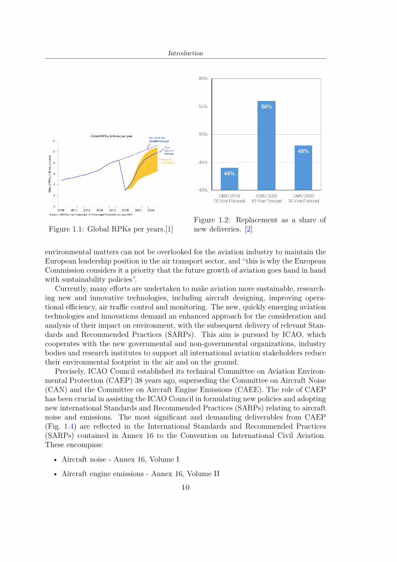
1.1 The environmental concernThe outbreak of Covid-19 pandemic has spread new uncertainties over the commercialaviation sector and has slow down the worldwide air transport growth. Nevertheless,a long-term increase in air traffic is expected. According to IATA outlook update toApril 2021 [1], once travel restriction are lowered, a strong rebound of travel shouldbe expected, leading to an increase in air traffic, even though at a slower pace thanexpected before 2019 (Fig. 1.1). Furthermore, an optimpistic perspective provided byBoeing suggests a greater confidence in the resilience of commercial aviation and ex-pects a significant increase in replacement as share of new deliveries (Fig. 1.2), focusedon a renew of airline fleets to provide future network flexibility, maximizing capabil-ity while minimizing risk, and improving efficiency and sustainability [2]. Therefore,the future increasing air traffic and the need for innovation in the aviation industryhave put greater emphasis on several aspects, such as operations, RAMS (Reliability,Availability, Maintenance and Safety) and economic and environmental sustainability,leading to the introduction of new constraints in the aircraft design process.
Among these, the rise in public awareness has made the environmental requirementsthe most pressing issues hampering commercial aviation growth today. As stated byVioleta Bulc, the European commissioner for transport, in the European AviationEnvironmental Report [3], the demand from EU citizens for air travel is expected togrowth, “but growth for the sake of growth cannot be an objective in itself”, since
9
Introduction
Figure 1.1: Global RPKs per years.[1]Figure 1.2: Replacement as a share ofnew deliveries. [2]
environmental matters can not be overlooked for the aviation industry to maintain theEuropean leadership position in the air transport sector, and “this is why the EuropeanCommission considers it a priority that the future growth of aviation goes hand in handwith sustainability policies”.
Currently, many efforts are undertaken to make aviation more sustainable, research-ing new and innovative technologies, including aircraft designing, improving opera-tional efficiency, air traffic control and monitoring. The new, quickly emerging aviationtechnologies and innovations demand an enhanced approach for the consideration andanalysis of their impact on environment, with the subsequent delivery of relevant Stan-dards and Recommended Practices (SARPs). This aim is pursued by ICAO, whichcooperates with the new governmental and non-governmental organizations, industrybodies and research institutes to support all international aviation stakeholders reducetheir environmental footprint in the air and on the ground.
Precisely, ICAO Council established its technical Committee on Aviation Environ-mental Protection (CAEP) 38 years ago, superseding the Committee on Aircraft Noise(CAN) and the Committee on Aircraft Engine Emissions (CAEE). The role of CAEPhas been crucial in assisting the ICAO Council in formulating new policies and adoptingnew international Standards and Recommended Practices (SARPs) relating to aircraftnoise and emissions. The most significant and demanding deliverables from CAEP(Fig. 1.4) are reflected in the International Standards and Recommended Practices(SARPs) contained in Annex 16 to the Convention on International Civil Aviation.These encompass:
• Aircraft noise - Annex 16, Volume I
• Aircraft engine emissions - Annex 16, Volume II
10

1.2 – Sustainable supersonic flight
• Aeroplane CO2 emissions - Annex 16, Volume III
• Carbon Offsetting and Reduction Scheme for International Aviation (CORSIA) -Annex 16, Volume IV
Figure 1.3: CAEP deliverables. [4]
CAEP also developed various guidance materials that support States’ initiativestowards the environmental goals defined by the ICAO Assembly [4].
The activities of CAEP also provide for continuous monitoring and assessment ofaviation environmental matters, keeping its publications up to date, ensuring that thelatest environmental technologies are incorporated into new aircraft designs, and theenvironmental impact of international civil aviation is limited and reduced. Hence,despite the current downturn, the highly dynamic context of the air transport sectoris driving the aviation industry to attain ever rising economic, environmental, andsocial standards in the coming years. The achievement of these long-term objectives issupported by national and international agencies with the formulation of new SARPsand guidelines, that will involve the adoption of innovative air vehicle designs andsystematic changes to the manufacture and operation of aircraft, including the type offuel used, engine performance, weight metrics, air traffic management strategies andadvances in safety.
1.2 Sustainable supersonic flightRecent years have seen a revival of interest in supersonic aircraft and today there aremany projects under development that try to overcome the technological limits of afew decades ago to bring commercial supersonic civil transport flight back to reality.But why supersonic flight?
11

Introduction
As already mentioned, current market requirement is to have more efficient aircraft.Supersonic flight allows us to reduce the flight time and to reach increasingly longerpoint-to-point routes, with no need for stopovers. However, it was over two decade agowhen the last civil supersonic aircraft could be seen airborne. Since then, not only nopassenger supersonic airplane has taken off, but also the development of almost all su-personic airliners has been terminated. After the pioneering era of the first supersonicaircraft generation, such as Concorde and the Tupolev (Tu-144), aircraft manufactur-ers have mostly abandoned the idea of supersonic travelling, due to a broad range ofissues related to supersonic transport. Concorde was certainly a technological accom-plishment for its time, reaching a maximum cruising speed of 2179 km/h per hour withMach 2.04, allowing the aircraft to reduce the flight time between London and NewYork to about three hours. Despite of this, its environmental and operational limita-tions hindered the achievement of the success its creators had hoped for. Beyond thehigh production cost, the problems of the Concorde consisted in the high consump-tion (about 13 litres/100 km per seat) and noise emissions, associated with take-offand sonic boom. Sonic boom occurred when Concorde flew faster than the speed ofsound and the thunderous sound was caused by series of shock waves coming from theaircraft’s nose, wings and engines. It rattled and broke windows and also frightenedboth humans and animals. That is why Concorde planes were never permitted to flyat full and supersonic speeds over land, as they were restricted to subsonic speeds onland. On July 25 in 2000, a Concorde en route from Paris to New York City sufferedengine failure shortly after take-off, when debris from a burst tire caused a fuel tankto rupture and burst into flames. The aircraft crashed into a small hotel and restau-rant. All 109 persons on board, including 100 passengers and 9 crew members, died;4 people on the ground were also killed. Considering the economic failure, on October24 in 2003 the Concorde was definitively retired and any supersonic passenger aircraftprojects were shut down. Clearly, the possibility of future development of SuperSonicTransport (SST) is closely connected with solving related environmental problems.
After a few decades, aviation technology has considerably advanced and the avia-tion industry is ready to face the challenges of supersonic flight and overcome them,welcoming a new generation of SST aircraft. The National Aeronautics and SpaceAdministration (NASA) in partnership with Lockheed Martin is currently working onthe development of a low-boom flight demonstrator known as X-59 Quiet SuperSonicTechnology (QueSST)(Fig. 1.4). X-59 QueSST is an experimental supersonic aircraftwhich preliminary design started in February 2016, with the scheduled for delivery inlate 2021 for flight tests from 2022. It is expected to cruise at Mach 1.42, creating alow 75 Perceived Level decibel (PLdB) thump to evaluate supersonic transport accept-ability. The demonstrator aims to fly in the 2020 timeframe and the data gatheredmay open the future to commercial supersonic flight over land.
12

1.2 – Sustainable supersonic flight
Figure 1.4: Low-boom flight demonstrator X-59 QueSST.
A further step forward has been done by Denver-based aerospace company BoomTechnology, with the development of XB-1, a 1/3 scale demonstrator, and Overture(Fig. 1.5), a 55-passenger sustainable supersonic airliner with 8300 Km of range, thataims to fly at Mach 1.7, optimized to run on 100% sustainable aviation fuel (SAF) withnet-zero carbon emissions. Since 3rd June 2021, the United Airlines have announceda commercial agreement with Boom Supersonic to add 15 aircraft to its global fleet.Under the terms of the agreement, United will purchase 15 Overture airliners, onceOverture meets United’s demanding safety, operating and sustainability requirements,with an option for an additional 35 aircraft. Overture is slated to roll out in 2025, flyin 2026 and expected to carry passengers by 2029 [5].
Figure 1.5: Future supersonic airliner Overture.
13

Introduction
Meanwhile, Boston-based Spike aerospace is focusing on the development of SpikeS-512 (Fig. 1.6), a supersonic business jet flying at Mach 1.6 and intended for privateuse.
Figure 1.6: Future supersonic business jet Spike S-512.
These technological advances suggest that a new era of enduring supersonic flight isclose. However, the lack of agreed-upon international standards or agreements is likelyto hinder production as well as operations [6]. Since 1973 United States and othercountries have banned supersonic flight over land, except in limited circumstances,because the annoyance due to sonic boom exposure was considered unacceptable for thepublic. Consequently, such restriction has severely limited the viability of supersonicflight and has compromised its economic competitiveness, increasing operating costsand flight times. At present, sonic boom reduction measures have been included in thedesigns of the new SST aircraft, but no change has been introduced in the regulationfrom the times of Concorde. For this reason, an investigation about the acceptablelevels of sonic boom and the establishment of a univocal and homogeneous regulationare the indispensable premise for the new SST aircraft to fly and go faster than sound.
1.2.1 Noise acceptability and regulationThe main regulatory issues related to supersonic flight arise from limitations imposedby community noise levels acceptability. Noise annoyance in the vicinity of airport isa problem concern both subsonic and supersonic aircraft. Since 1960s aircraft noisewas recognized as a serious environmental pollutant. The growth of jet-powered fleetand the increasing air traffic revealed the necessity to set local mandatory noise limitsaround the airport, thus the government started to introduce the concept of noise cer-tification, whose requirements were made much more stringent and were more widelyapplied during the following years [7]. Such a tightening has been due to an increasing
14

1.2 – Sustainable supersonic flight
public awareness and a significant transnational political attention about the magni-tude of the environmental problem and the effects of pollution on human beings, asair traffic has increased more and more. The findings collected from social surveysand research activities draw attention to noise adverse effects on the health of exposedindividuals: exposure to aircraft noise and the health indicators claiming that subjectswho have been chronically exposed to high aircraft noise level are more likely to reportstress, sleep disturbance and hypertension compared with those not exposed to aircraftnoise [8],[9],[10].
During the years, health-based guidelines on community noise have driven the for-mulation of noise standards within a framework of noise management to safeguard thehealth of airport neighbours through appropriate regulation of LTO noise levels. How-ever, the incoming supersonic fligh presents regulatory authorities with a new challenge.A supersonic aircraft taking-off significantly exceeds noise levels of subsonic passengeraircraft, as the greater jet speed of supersonic engine has a large influence on noisegeneration. Looking at the Figure 1.7, the Concorde represents a good example ofthe additional noise associated with supersonic aircraft compared to subsonic aircraft.Among the noise levels produced by the aircraft enetered into service between 1955and 1990, it can be observed that the average noise levels of more recent subsonic air-craft decreased considerably (by more than 20 EPNdB), but Concorde produced morenoise than the loudest jet aircraft. These differences can only be explained by the largedifference in design requirements between supersonic and subsonic aircraft [11].
Figure 1.7: Jet aircraft noise levels at entry into service until 1990. [11]
For this reason, a more specific understanding of airport noise impacts resulting fromthe introduction of SST aircraft is needed. Current noise provisions defined in ICAOAnnex 16, Vol.I [12] recommended to take SARPs defined for subsonic jet airplanes asguidelines for Landing and Take-Off (LTO) noise requirements of the new generationSST aircraft. As previously said, aircraft noise standards have become much stricter
15

Introduction
since the Concorde entered service. The introduction of Turbofan engines with highby-pass ratio and further noise reduction technologies incorporated into engine andairframe designs led to incremental improvements in aircraft noise performance andincreasingly stringent noise standards, that currently are reported in Chapter 14 ofAnnex 16, Vol I ( 1.8).
Figure 1.8: The progression of the ICAO LTO noise Standards for aeroplanes – Cu-mulative noise limits vs. Maximum Take-Off Mass (MTOM). [13]
Aircraft noise limits for LTO cycle are defined by ICAO as Effective Perceived NoiseLevels (EPNL). The EPNL is a noise evaluator for the noisiness due to an aircraft pass-by, accounting for effects on human beings and consisting of an integration over noiseduration of the Perceived Noise Level (PNL), normalized to a reference duration of 10seconds. The noise levels for certification are associated with three different operatingconditions of the engines, each of which corresponds to the definition of a groundreference measurement point:
• Lateral full-power reference noise measurement point (maximum power condition):the measurement point is along the line parallel to the axis of runaway centre lineat a distance of 450 m, where the noise level is maximum during take-off.
• Flyover reference noise measurement point (intermediate power condition): themeasurement point is along the extended runaway centre line at a distance of6500 m from the start to roll.
• Approach reference noise measurement point (low power condition): the measure-ment point on the ground it is along the extended runaway centre line at 2000 mfrom the threshold. This corresponds to a position 120 m vertically below the 3°descent path originating from a point 300 m beyond the threshold.
The reference measurement points are respectively lateral (or sideline), flyover (orcutback) and approach reference point, as represented in Figure ( 1.9).
16

1.2 – Sustainable supersonic flight
Figure 1.9: Aircraft noise certification reference measurement points. [20]
Noise is recorded continuously at these locations during take-off and landing. Thetotal time-integrated noise, i.e. the EPNL, must not exceed a set limit, establishedaccording to MTOW and number of engines, as specified in Attachment A of ICAOAnnex 16, Vol.I. Within Annex 16, Vol. I Chapter 3 (Chapter 14 refers to this chapter),in addition to the definition of the three noise measurement points based on the enginepower levels, the noise certification reference procedures are also reported. These definethe mass, thrust levels, speeds and configuration that the aircraft must have for take-off and approach, respectively for the noise measurement at the sideline and cutbackreference measurement point and approach reference measurement point.
Another noise concern of supersonic aircraft is the sonic boom generated duringsupersonic cruise. When an aircrfat flies faster than sound, it creates a series of pressurewaves that travel at the speed of sound and, as the aircraft speed increases, the wavesare compressed together. At very large distances from the body, the wave system tendsto distort and steepen, ultimately coalescing into a bow and a tail wave. The Figure1.10 shows a schematic diagram representing the typical far-field wave patterns. Atthe bow wave a compression occurs in which the local pressure p rises to a value ∆pabove atmospheric pressure. Then, a slow expansion occurs until some value belowatmospheric pressure is reached, after which there is a sudden recompression at thetail wave. This nominal sonic boom signature is called an N-wave. It moves with theaircraft and is associated with continuous supersonic flight, not just with “breaking thesound barrier.” One speaks of a sonic boom “carpet”, whose width depends on flightand atmospheric conditions, swept out under the full length of a supersonic flight.Receivers within the carpet detect the sonic boom, that is the N-wave once as theaircraft passes. If these waves were sweeping by an observer on the ground, the ear’saural response would be as shown schematically in the sketch at the bottom of theFigure 1.10. Since the duration of this wave signal usually is less than 0.1 second, thepressure rises are heard as a single bang.
In a future scenario, where SST aircraft will be able to fly, this thunderous noise
17

Introduction
Figure 1.10: Sonic boom pressure far-field wave patterns.[15]
level needs to be regulated. However, whereas supersonic LTO noise standard hasdefined in accordance with subsonic ones, no regulations have yet been establishedfor regulating sonic boom levels during supersonic flight. The latest ICAO resolutionabout limitations of enroute flight of the SST aircraft dates back to 1998 and aims atensuring that no unacceptable situation for the public is created by sonic boom fromsupersonic aircraft in commercial service. In the following years, the work on civilsupersonic development programs and research initiatives has led ICAO to intensify itsefforts towards creating a comprehensive regulatory framework for future supersonicaircraft, identifying certification measurement locations and noise metrics for assess-ing sonic boom noise on the ground and evaluating the benefits of using sonic boompredictions in supersonic noise certification in addition to physical measurements. Aset of exploratory studies and research programs are supporting ICAO activities tomake the certification of a supersonic aeroplane possible in the 2020-2025 timeframe.A relevant example is RUMBLE (RegUlation and norM for low sonic Boom LEvels), athree-year program sponsored by the European Commission and the Russian Federa-tion, that seeks to address both technical and regulatory aspects of sonic booms. Themain actions of the project are:
• Development and assessment of sonic boom prediction tools.
• Study of the human response to sonic boom.
• Validation of the findings using wind-tunnel experiments and actual flight tests
RUMBLE activities are dedicated to the production of the scientific evidence re-quested by national, European and international regulation authorities to determinethe acceptable level of overland sonic booms and the appropriate ways to comply withit [14]. Ultimatly, work is ongoing in civil aviation authorities, industries and researchinstitutes to achieve greater awareness of the environmental impact of future supersonicaircraft and develop a specific regulation that overcomes the current lack, allowing thecertification of supersonic aircraft as soon as possible.
18

1.3 – Research goal
1.3 Research goalNoise levels restrictions imposed in the vicinity of airport and over populated areasconstitute the main regulatory issue surrounding civil supersonic flight. Therefore,focusing on LTO noise, the presented work addresses the development of a methodologyaimed at including noise requirements as a design constraint in the early stages of SSTaircraft. Such purpose is placed in the scenario of the "Balanced approach", proposed byCAEP in the field of aircraft noise management. Such approach consists of identifyingthe noise problem at an airport and analysing the various measures available to reducenoise through the exploration of four principal elements, namely reduction at source,land-use planning and management, abatement operational procedure and operatingrestrinctions, with the goal of addressing noise in the most cost-effective manner [15].
In this context, the developed methodology could be able to gain a better under-standing of noise requirements on the aircraft design process and support the reductionof noise at source, through the analysis of the relationship between noise and aircraftdesign and operational parameter and the identification of guidelines to include noisereduction measures into aircraft design, promoting a design-to-noise approach.
The main objectives of the presented activities are:
• To demonstrate the feasibility of introducing noise emission estimation at concep-tual design level and identify design and performance parameters which might beimpacted by noise requirements.
• To validate the developed methodology with experimental data and assess itsaccuracy in noise prediction.
• To show an application to departure and approach procedures, testing the abilityof the methodology in the evaluation of the noise levels at the three certificationnoise measurement points.
The progression followed in order to achieve these objectives is summed up in theroadmap in the Figure 1.11. The activities performed can be considered as split intotwo parts. Firstly, an in-depth research activity about methods for modelling andpredicting aircraft noise has been conducted in order to classify the different method-ologies currently adopted for aircraft noise prediction purposes and to achieve an un-derstanding of the general requirements of avaiable state of art tools. After that, asemi-empirical approach has been selected as the most appropriate for applications ata conceptual design level. Hence, an SST aircraft noise model based on Aircraft NOisePrediction Program (ANOPP) equations has been developed and employed througha set of Matlab routines. At least, the noise model has been integrated within theoverall methodology framework, that encompasses other routines involving engine op-eration modelling, flight path simulation, atmospheric absorption effect and calculationof noise metrics. Chapter 2 and Chapter 3 of the thesis cover these arguments.
Secondly, once the methodology has been developed, it was used to assess SSTaircraft noise levels and the results were discussed. Chapter 4 and Chapter 5 deals
19

Introduction
Figure 1.11: Roadmap of the activities performed in the thesis.
with its application and give an example of its noise prediction capabilities integratedwithin conceptual design. The Matlab program has been run for flyover trajectoriesat different thrust ratings and altitudes to perform a dedicated validation with experi-mental data provided by Aircraft Noise and Performance (ANP) database, consideringboth instantaneous and integrated noise metrics. The only available SST aircraft ofthe ANP, i.e. the Concorde, has been selected as case study. The results obtainedhave shown an acceptable level of accuracy for applications at a conceptual designlevel, leaving options open to gain a higher fidelity-level with further improvementsand correction in noise prediction and engine modelling. Furhtermore, fixed-pointdata provided by ANP have been employed to simulate trajectories for departure andapproach procedures to predict noise level at the certification points during LTO cycle.The outcome of the work demonstrated the capability of the developed methodologyto be applied for evaluating the noise requirements since the early stages of aircraftdesign and providing useful guidelines for the design of future low-noise SST togetherwith operational procedures able to mitigate the LTO noise.
A synthesis of the objectives achieved is reported in the concluding Chapter, withconsiderations regarding possible improvements and future developments.
20

Chapter 2
Noise source modelling
The Chapter addresses the noise source modelling starting from an assessment of stateof art in aircraft noise prediction. Hence, a literature review on current methodsand tools availables to model and predict aircraft noise is presented, focusing on themost relevant under the scope of this thesis, i.e. Aircraft NOise Prediction Programdeveloped by NASA. After that, the SST aircraft LTO noise model employed is de-scribed, providing the noise sources breakdown and the relative equations to eachsub-components of overall noise. Lastly, the model has been implemented in differentMatlab routines and results obtained have been reported.
2.1 Literature review
Currently, many tools and methods are available to account for environmental sus-tainability requirements as project constraints in the early design of the aircraft andmission, aiming at reducing the environmental impact and/or operating costs. A num-ber of optimization studies towards different objectives can be found in the literature,e.g. [17], [18], [19]. Such activities usually include the application of a noise predictionsoftware, in order to assess the environmental impact of an overall aircraft system. Inthe sphere of the overall aircraft noise prediction, several computer programs are widelyused, according to the application background. An exaustive classification about thestate of art in aircraft noise prediction is presented in [20], [21], [22]. Possible methosadopted to model and predict aircraft noise are listed below:
• Fully analytical: both the fluid mechanic and acoustic results used in the analysisare obtained analytically. Despite the high efficiency of these methods, theyare suitable only for simple models and basic research. Modelling aircraft noisesources with a fully analytical approach is not recommended, as the problemhas multidisciplinary implications and involves an advanced knowledge of fluiddynamics, acoustic and mathematics.
21

Noise source modelling
• CFD combined with acoustic analogy: these methods involve turbulent simulationin the near field, determining the acoustic propagation from aerodynamic flow cal-culation. The main shortcoming of the analytical methos is partially overcome, asCFD are able to model more complex sources. However, these methods, especiallyfully CFD, often require high computational time.
• Scientific: typically based on some empirical data and on an adeguate physicalmodel for noise generation mechanism, these methods provide a parametric sourcedefinition that allows to account for the impact of operational settings and air-frame/engine geometry on noise generation. Their strength relies on the reliabilityof the results obtained in a certain field of validity, without excluding the possi-bility to extend the prediction also outside it and explore the noise evaluation ofunconventional aircraft.
• Best practice: they rely almost exclusively on ground measurements of a specificaircraft. Then, the measured noise immission related to overall aircraft noise iscorrected accounting for propagation effect to determine the originating emissionnoise level of the aircraft. Best pratice methods allows a faster and more praticalapproach. However, their fidelity is restricted to the aircraft considered and thepredicted overall noise cannot be categorized into individual sub-components.
Scientific and best pratice are the most common methods used to predict overallaircraft noise. In the next paragraphs some examples of state of art tools relying onthese methods are given.
Scientific methods Namely also semi-empirical, componential or parametric, thesemethods are the most widely used for noise evaluation at a conceptual design level,as they are able to predict noise immission from both conventional and unconven-tional aircraft. Scientific noise prediction is furthermore characterized by a parametricmodelling of each individual noise source. Such a parametric formulations enable theprediction of the various effects on noise radiation caused by the variations of aircraftconfiguration and operating conditions throughout simulated flight operations. Suchmodels capture the major physical effects and correlations yet allow for a fast noiseprediction. Thus, many efforts have been undertaken for the development of noiseprediction methodologies based on a semi-emprical approach The most relevat exam-ple of this kind of tools is Aircraft NOise Prediction Program (ANOPP), the firstcomputer program with noise prediction capabilities developed by NASA Langley Re-search Center in the early 1970s. One of the first major applications of ANOPP wasto support the Supersonic Cruise Research (SCR) project at Langley, while next ap-plication was in conjunction with the Federal Aviation Administration (FAA) study todetermine economically reasonable and technologically feasible noise limits for futuresupersonic transports [23]. NASA has been continuing its activity in this area, andhave announced a new release of the program with ANOPP2, whose purpose has beenextended to noise evaluation for unconventional aircraft configurations [24].
22

2.1 – Literature review
In recent years, also the German Aerospace Center (DLR) has developed anothernoise prediction tool, the Parametric Aircraft Noise Analysis Module (PANAM). Thecurrent version of PANAM is applicable to the noise evaluation of conventional aircraftconfigurations along arbitrary threedimensional flight trajectories. The PANAM frame-work allows for a straight forward integration of additional or updated noise sourcemodels reflecting progress in modeling the physics of noise source mechanisms andtheir parametrical dependencies. The modular setup allows for either self-containedoperation or for direct integration in a multidisciplinary design code such as the codepreliminary aircraft design and optimization developed at the Technical University ofBraunschweig, Germany. The PRADO integration allows for fully automated low noiseoptimization of aircraft configurations in the preliminary design process [25], [30].
Meanwhile, the University of Manchester has been developing FLIGHT, a programwith the aim of creating a reliable software framework for the current generation of com-mercial aircraft powered by gas turbine engines. Yet, unlike other computer models,this program does not address any issue of conceptual design. Indeed, it uses the frame-work, composed by different modules (geometry, aerodynamics, propulsion, airframe-engine integration, flight mechanics, trajectory optimisation, thermo-structural per-formance, static stability, parametric analysis and aircraft noise), to generate reliablemodels of the aircraft systems by using a composite method that relies on a large database with the aim of obtain a basis for model and noise validation. Also for this tool,the aircraft noise is modeled on the basis of the method of components, with someconsideration for interference factors between the sources [26].
Best pratice methods Tools that can be assigned to this category provide an eval-uation of medium to long term average noise levels around airports rather than forprediction of single flyover events and qualify for application in air traffic manage-ment and legislation processes. Typically best practice methods rely on Noise PowerDistance (NPD) experimental data for an individual aircraft. NPD relationships areobtained as a function of observer distance via spherical spreading through a standardatmosphere and represents the standard technique for evaluating noise from flight pro-cedures, accounting for modifications to flight path, runway/airport layout, and fleetmix on overall ground noise through the introduction of corrective factors. The firstexample of best practice tool is the Integrated Noise Model (INM) developed by FAA.In this case, noise prediction procedure is based on NPD data normalization to a spe-cific straight horizontal flight segments with constant operational and configurationalsetting. In this way, noise immission along a selected flight path is predicted assemblingthe corresponding trajectory from these straight flight segments [27]. The fixed-wingaircraft portion of the INM database is harmonized with ICAO’s Aircraft Noise andPerformance (ANP) database, which accompanies ECAC’s Doc 29 [28].
Another example of this tools, that may be defined as an hybrid approach, is SIMUL,another tool developed by DLR. The concept of SIMUL is a description of the aircraftas a sound source by a set of partial sound sources. This separation process is basedon the way the source mechanisms are influenced by the aircraft speed. The actualversion of the model describes the following separate mechanisms: jet nois is influenced
23

Noise source modelling
by the aircraft speed as well as the jet speed. The remaining sources of engine noise areinfluenced by aircraft speed only. SIMUL database is derived from measurements andmanufacturer information for engine model, wheareas is based on PANAM results forairframe noise. As a result, SIMUL represents a compromise between a pure empiricalmodel and a pure analytical model [29].
2.1.1 ANOPPAs already mentioned, ANOPP was the first computer program applicable to the pre-liminary design of the aircraft to elaborate and indicate where further theoretical andexperimental research on noise prediction is needed. NASA initiated the developmentof ANOPP approximately 50 years ago to support high-speed transport research pro-grams sponsored by U.S. goverament. The purpose of ANOPP first code was to predictnoise from an aircraft by accounting for the effects of its engines, its operations, theatmosphere including ground effects, and other characteristics which may influence thenoise it generates. The prediction methodologies implemented within the code wereempirical or semiempirical and relied on a widly available experimental data sets andacoustic prediction methods. Following a componential approach, overall aircraft noisewas computed as an assembly of each major noise sources. Indeed, an intensive researchhas been conducted during the years about noise prediction models for airframe andengine contributions (that are considered the most dominant aircraft noise sources)that underlie the overall noise prediction. However, the core of the program, that wasthe noise source model, interfaced with several other modules, in order to obtain a com-prehensive model for noise prediction. Precisely, "comprehensive" means that variousaspects of the aircraft are modelled in the code, such as main sub-systems and theirmutual integration, in order to offer a realistic simulation tool of the aircraft withoutthe need of too much detail on each system, which would be unavailable anyway [26].Hence, ANOPP embedded models for sound propagation from near the aircraft to-wards the observer on the ground, including the effects of the atmosphere and terrain,and installation effect, including scattering and shielding, and is integrated with otherperformance modules for flight dynamics and engine operations.
In ANOPP first version any of the prediction methods work well for conventionalaircraft configurations,but lack capability and fidelity required for non conventionalconfigurations. As a conquence, in 2011 NASA released the new version ANOPP2,including the tools of the older ANOPP version for engine and airframe noise andintroduces new tools with a higher level of fidelity for source noise component predic-tion, installation effects, and propagation to the far-field in order to predict noise forunconventional designs [24]. However, ANOPP2 incorporates the same fundamentalconcepts of the first version, with improvements in terms of reliability, accuracy andvalidity of the results. Therefore, it is possible to say that starting from the first versionof the program, ANOPP constitutes a guideline in the development of comprhensivemethodologies for the prediction of noise, differing essentially only for the models em-ployed. To understand the program concept, a description of noise evaluation problemis necessary (Fig. 2.1).
24

2.1 – Literature review
Once aircraft noise emission has been predicted in terms of Sound Pressure Level(SPL) for a given instant of time and in a single point of the trajectory, the integrationwith aircraft flight dynamics lead to the extension of noise prediction along the flightpath. The estimation obtained is not yet the noise that the observer on ground receive,as propagation effects from atmosphere and ground have to be accounted for. It is clearthat aircraft noise evaluation alog a trajectory involves different parameters related toaircraft operation and configuration and ambient condition.
Figure 2.1: Aircraft noise prediction problem [23].
The ANOPP System is divided into two parts: the executive system and thefunctional module library. The executive system controls execution of the program, whereas the functional module library contains all of the research functional mod-ules. Each functional module is an independent group of subprograms which performsnoise prediction functions. A flow chart of the ANOPP system functional module isshown in Fig. 2.2. The procedure begins by defining an atmosphere using the At-mosphere Module (ATM), followed by the atmospheric absorption module (ABS). Thesteady flyover module (SFO) is used for the approach measurement point, and the jettakeoff module (JTO)for sideline and takeoff measurement points. The geometry mod-ule (GEO) computes the range and directivity angles from the observer to the noisesource. At this point, the various noise sources modules are run: Heidmann’s18 for fannoise (HDNFAN), Stone’s19 for coaxial jet noise (STNJET) and Fink’s20 for airframenoise (FNKAFM). Once data has been generated by the noise source modules, thepropagation module (PRO) applies corrections to the noise data in the source frameof reference to transfer it to the observer frame of reference. Atmospheric absorptioneffects are applied at this point. The noise levels module (LEV) computes the tonecor-rected Perceived Noise (PNLdB),and the effective noise level module (EFF)is run nextto compute the EPNdB levels used as noise metrics in this research [24].
ANOPP has also been extended to a high-speed research program with the AircraftNoise Prediction Program’s High Speed Research prediction system (ANOPP-HSR),including modules to serve particular prediction requirements relative to high-speed
25

Noise source modelling
Figure 2.2: Flow chart of ANOPP functional modules.[24].
aircraft [31]. Hence, under the scope of this work, ANOPP has been taken as a ref-erence, since it is considered an example of a comprehensive methodology for aircraftnoise prediction, suitable also for SST aircraft.
2.2 SST aircraft LTO noise modelThe method of components has become the prevalent method for predicting aircraftnoise. Such method relies on the typical distiction of aircraft noise in propulsive andnon propulsive (airframe) sources. In turn, these two contributions are broken downinto other sub-components depending on design and operational parameters. In orderto identify the noise sub-components for a supersonic aircraft leading to the generationof noise during take-off and landing, a comparison between subsonic and supersonicaircraft has been considered. In general, neglecting interaction and installation effects,aircraft components listed and described in Tables A.1 and A.2 (Appendix A) can beconsidered the main noise sources for a subsonic aircraft.
The main differences between subsonic and supersonic aircraft are exhaustivelydescribed in [11] and are summed below:
• The wing shape: even thought this is the most visible physical difference be-tween subsonic and supersonic aircraft, it has not much influence on the totalnoise generated. Clean wing noise is mainly due to the turbolence generation attrailing egde, thus the most influential parameters are velocity, wing span andboundarylayer thickness.
26
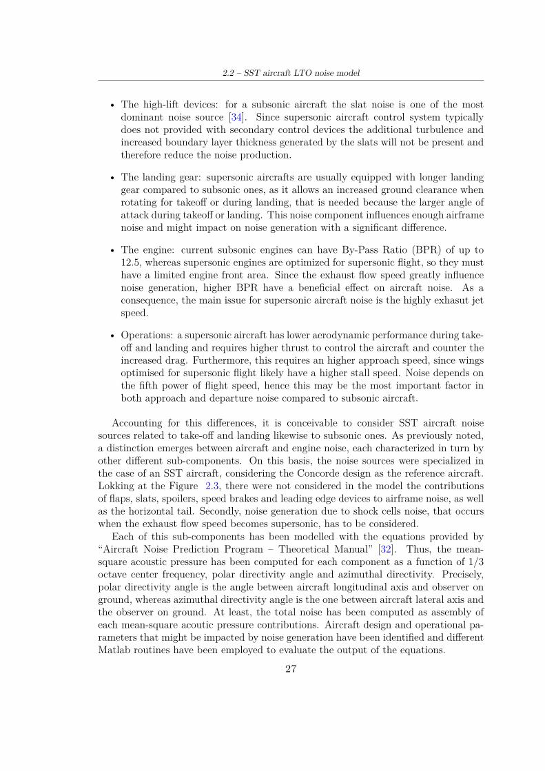
2.2 – SST aircraft LTO noise model
• The high-lift devices: for a subsonic aircraft the slat noise is one of the mostdominant noise source [34]. Since supersonic aircraft control system typicallydoes not provided with secondary control devices the additional turbulence andincreased boundary layer thickness generated by the slats will not be present andtherefore reduce the noise production.
• The landing gear: supersonic aircrafts are usually equipped with longer landinggear compared to subsonic ones, as it allows an increased ground clearance whenrotating for takeoff or during landing, that is needed because the larger angle ofattack during takeoff or landing. This noise component influences enough airframenoise and might impact on noise generation with a significant difference.
• The engine: current subsonic engines can have By-Pass Ratio (BPR) of up to12.5, whereas supersonic engines are optimized for supersonic flight, so they musthave a limited engine front area. Since the exhaust flow speed greatly influencenoise generation, higher BPR have a beneficial effect on aircraft noise. As aconsequence, the main issue for supersonic aircraft noise is the highly exhasut jetspeed.
• Operations: a supersonic aircraft has lower aerodynamic performance during take-off and landing and requires higher thrust to control the aircraft and counter theincreased drag. Furthermore, this requires an higher approach speed, since wingsoptimised for supersonic flight likely have a higher stall speed. Noise depends onthe fifth power of flight speed, hence this may be the most important factor inboth approach and departure noise compared to subsonic aircraft.
Accounting for this differences, it is conceivable to consider SST aircraft noisesources related to take-off and landing likewise to subsonic ones. As previously noted,a distinction emerges between aircraft and engine noise, each characterized in turn byother different sub-components. On this basis, the noise sources were specialized inthe case of an SST aircraft, considering the Concorde design as the reference aircraft.Lokking at the Figure 2.3, there were not considered in the model the contributionsof flaps, slats, spoilers, speed brakes and leading edge devices to airframe noise, as wellas the horizontal tail. Secondly, noise generation due to shock cells noise, that occurswhen the exhaust flow speed becomes supersonic, has to be considered.
Each of this sub-components has been modelled with the equations provided by“Aircraft Noise Prediction Program – Theoretical Manual” [32]. Thus, the mean-square acoustic pressure has been computed for each component as a function of 1/3octave center frequency, polar directivity angle and azimuthal directivity. Precisely,polar directivity angle is the angle between aircraft longitudinal axis and observer onground, whereas azimuthal directivity angle is the one between aircraft lateral axis andthe observer on ground. At least, the total noise has been computed as assembly ofeach mean-square acoutic pressure contributions. Aircraft design and operational pa-rameters that might be impacted by noise generation have been identified and differentMatlab routines have been employed to evaluate the output of the equations.
27

Noise source modelling
Figure 2.3: SST aircraft LTO noise sources breakdown.
Assumptions In order to develop a noise prediction model suitable to conceptualdesign evaluations several approximations have been made:
• Each noise source is assumed to be independent, hence interaction and installationeffects are neglected.
• Noise scattering, reflection and shielding effects are not considered.
• The aircraft is assumed to be a lumped mass and all the acoustic sources areconcentrated on the airplane’s centre of gravity.
• Flap and slat noise are not present due to supersonic aircraft design considered.
• Turbomachinery and combustion noise are neglected.
2.2.1 Airframe noiseA review of several airframe noise prediction schemes is reported in [?], but that dueto Fink is the one most widely accepted as correct in its combination of a wide rangeof full-scale and model data. Accordingly, this work presents the main points of Fink’sproposals following mathematical formalism implemented in ANOPP. Considering ageneric subsonic aircraft, in Fink’s component method applied in [35] the overall air-frame noise is assembled as a combination of these individual models:
• Clean wing and tail surfaces noise
• Landing gear noise
• Trailing edge flap noise
• Leading edge slat and flap noise
28
2.2 – SST aircraft LTO noise model
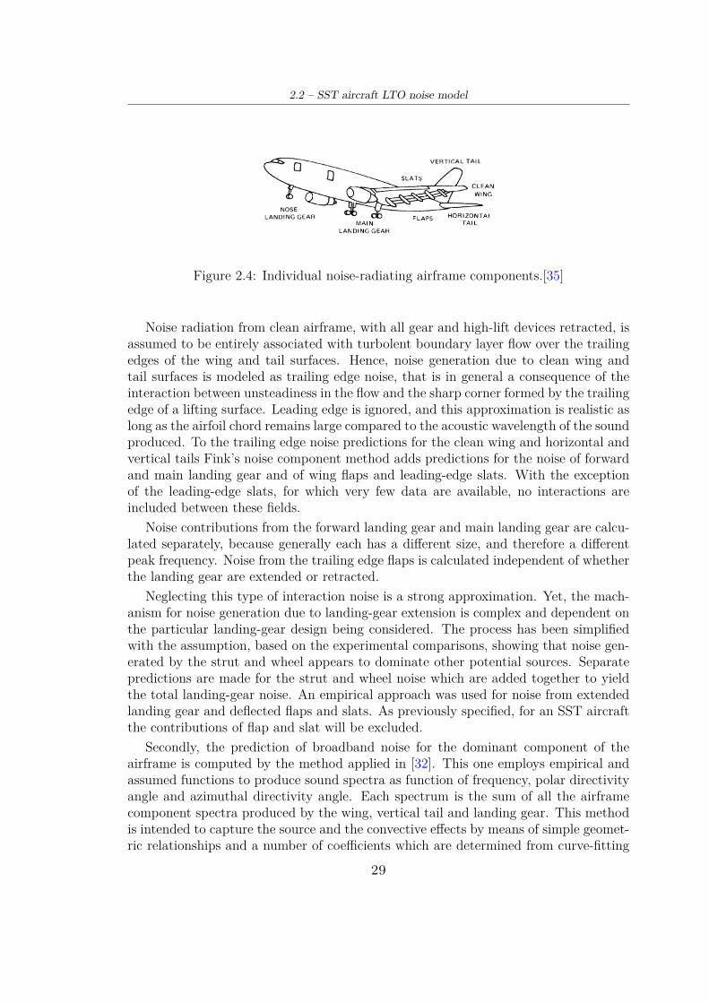
Figure 2.4: Individual noise-radiating airframe components.[35]
Noise radiation from clean airframe, with all gear and high-lift devices retracted, isassumed to be entirely associated with turbolent boundary layer flow over the trailingedges of the wing and tail surfaces. Hence, noise generation due to clean wing andtail surfaces is modeled as trailing edge noise, that is in general a consequence of theinteraction between unsteadiness in the flow and the sharp corner formed by the trailingedge of a lifting surface. Leading edge is ignored, and this approximation is realistic aslong as the airfoil chord remains large compared to the acoustic wavelength of the soundproduced. To the trailing edge noise predictions for the clean wing and horizontal andvertical tails Fink’s noise component method adds predictions for the noise of forwardand main landing gear and of wing flaps and leading-edge slats. With the exceptionof the leading-edge slats, for which very few data are available, no interactions areincluded between these fields.
Noise contributions from the forward landing gear and main landing gear are calcu-lated separately, because generally each has a different size, and therefore a differentpeak frequency. Noise from the trailing edge flaps is calculated independent of whetherthe landing gear are extended or retracted.
Neglecting this type of interaction noise is a strong approximation. Yet, the mach-anism for noise generation due to landing-gear extension is complex and dependent onthe particular landing-gear design being considered. The process has been simplifiedwith the assumption, based on the experimental comparisons, showing that noise gen-erated by the strut and wheel appears to dominate other potential sources. Separatepredictions are made for the strut and wheel noise which are added together to yieldthe total landing-gear noise. An empirical approach was used for noise from extendedlanding gear and deflected flaps and slats. As previously specified, for an SST aircraftthe contributions of flap and slat will be excluded.
Secondly, the prediction of broadband noise for the dominant component of theairframe is computed by the method applied in [32]. This one employs empirical andassumed functions to produce sound spectra as function of frequency, polar directivityangle and azimuthal directivity angle. Each spectrum is the sum of all the airframecomponent spectra produced by the wing, vertical tail and landing gear. This methodis intended to capture the source and the convective effects by means of simple geomet-ric relationships and a number of coefficients which are determined from curve-fitting
29

Noise source modelling
of empirical data. In spite of the theoretical shortcomings, specifically the misunder-standing that most of the noise was generated at the trailing edge, this method remainswidely used and (until recently) seldom criticised [22].
The general approach for each contribution is the same and is based on the followingequation for the calculation of the far-field acoustic mean-square pressure:
< p2 >∗= Π∗
4π(r∗s)
D(θ, φ)F (S)(1 − M∞ cos θ)4 (2.1)
Where:
• < p2 >∗: dimensionless mean-square acoustic pressure, re ρ2∞c4
∞
• Π∗: dimensionless overall acoustic power, re ρ∞c3∞b2
w
• D(θ, φ): directivity function
• F (S): spectrum function
• S: Strouhal number
• r∗s : dimensionless distance from source to observer, re bw
• (1 − M∞ cos θ)4: Doppler factor, that accounts the forward velocity effect
• θ: polar directivity angle, deg
• φ: azimuthal directivity angle, deg
With ρ∞ ambient density in [Kg/m3], c∞ ambient speed of sound in [m/s] and M∞aircraft Mach number; 4π(r∗
s) is a spherical propagation factor. The Strouhal numberS is defined as:
S = fL
M∞c∞(1 − M∞ cos θ) (2.2)
Where L is some length scale characteristic of the particular airframe noise sourcebeing computed. The acoustic power for the airframe Π∗ can be expressed as:
Π∗ = K(M∞)aG (2.3)
Where:
• K and a are constants determined from empirical data.
• G is a geometry function different for each airframe component and incorporatedall geometry effects on the acoustic power.
30
2.2 – SST aircraft LTO noise model
Source K a GClean wing 7.075 · 10−6 5 δ∗
w
(aerodinamically clean)Vertical tail 7.075 · 10−6 5 δ∗
v( bvbw
)2
(aerodinamically clean)1-and-2 wheel landing 4.349 · 10−4 6 n( d
bw)2
gear wheel noise4 wheel landing 3.414 · 10−4 6 n( d
bw)2
gear wheel noiseLanding gear 2.753 · 10−4 6 ( d
bw)2( l
d)strut noise
Table 2.1: K, a and G for each airframe noise component for SST aircraft. [32]
The values of K, a and G for this case study are reported in the Table 2.4 for eachairframe noise component.
Clear wing and vertical tail are considered as aerodinamically clean, such as asailplane or a jet aircraft with simple trailing edge flap mechanism. Moreover, forlanding gear, n, d and l are respectively the number of wheels per landing gear, thetire diameter and the struct length. The parameter δ∗ is the dimensionless turbolentboundary-layer thickness, computed from the standard flat-plate turbolent boundary-layer model, defined as:
δ∗ = 0.37 A
b2 (ρ∞M∞c∞A
µ∞b)−0.2 (2.4)
Where A and b are the wing surface and the wing span, chosen appropriately forthe wing or tail surface, wheares µ∞ is the ambient dynamic viscosity. Each airframenoise source has its own directivity function and spectrum function, listed in the table2.5; in the table 2.6 Strouhal number for each contribuition is reported.
Using these functions and the acoustic power, the mean-square acoustic pressurecan be computed as a function of frequency, polar directivity angle and azimuthaldirectivity angle for a given set of input parameters.
31

Noise source modelling
Source Directivity Spectrum functionClean delta wing 4 cos2 φ cos2 θ
2 0.485(10S)4[(10S)1.35 + 0.5]−4
Vertical tail 4 sin2 φ cos2 θ2 0.613(10S)4[(10S)1.5 + 0.5]−4
1-and-2-wheel landing 32 sin2 θ 13.59S2(12.5 + S2)−2.25
gear wheel1-and-2-wheel landing 3
2 sin2 θ sin2 φ 5.32S2(30 + S8)−1
gear strut4 wheel landing 3
2 sin2 θ 0.0577S2(1 + 0.25S2)−1.5
gear wheel4 wheel landing 3
2 sin2 θ sin2 φ 1.280S3(1.06 + S2)−3
gear strut
Table 2.2: Directivity function D and Spectrum function F (S) for each airframe noisecomponent for SST aircraft [32]
Source Strouhal number S
Clean delta wing fδ∗wbw
M∞c∞(1 − M∞ cos θ)
Vertical tail fδ∗vbv
M∞c∞(1 − M∞ cos θ)
1-and-2-wheel landing fdM∞c∞
(1 − M∞ cos θ)gear wheel
1-and-2-wheel landing fdM∞c∞
(1 − M∞ cos θ)gear strut
4 wheel landing fdM∞c∞
(1 − M∞ cos θ)gear wheel
4 wheel landing fdM∞c∞
(1 − M∞ cos θ)gear strut
Table 2.3: Strouhal number S for each airframe noise component for SST aircraft [32]
32

2.2 – SST aircraft LTO noise model
2.2.2 Engine noiseNoise generated by engine consists of several contributions, which in literature aregenerally classified into: fan noise, jet noise and engine core noise (compressor stages,combustor, turbine stages), as depicted in Figure 2.5.
Figure 2.5: Summary of engine noise sources (General Electric Affinity by GE Aviation- Turbofan for supersonic transport)
ANOPP provides different modules capable to predict each contribution:
• Fan noise: predicts the broadband noise and pure tones for an axial flow compres-sor or fan. The method is based on the method developed by M. F. Heidman.
• Combustion noise: predicts the noise from conventional combustors installed ingas turbine engines. The method is based on that one proposed by SAE ARP876.
• Turbine noise: predicts the broadband noise and pure tones for an axial flowturbine. The method is based on a method developed by the General ElectricCompany.
• Single stream circular jet noise: predicts the single stream jet mixing noise fromshock-free circular nozzles, on the basis of SA ARP 876.
• Circular jet shock cell: predicts the broadband shock-associated noise from asingle convergent nozzle operating at supercritical pressure ratios, on the basis ofmethod proposed by SAE ARP 876.
• Stone jet noise: predicts the far-field mean-square acoustic pressure for singlestream and coaxial circular jets. Included in the prediction are both jet mixingnoise and shock-turbulence interaction noise, on the basis of Stone method. Forcoaxial nozzles, the method is limitedto jets whose core jet velocity is greater thanthe secondary jet velocity. Further, only the core jet velocity may be supersonic.
33

Noise source modelling
• Dual stream coannular jet noise: predicts the noise characteristics of a coannularjet exhaust nozzle with an inverted velocity profile.
Yet, considering the large amount of data required to compute each contribution, ata conceptual design level it is conceivable to account only for the two most predominantnoise sources, which are fan and jet noise. Furthermore, a distinction must be madeamong the different types of engine that could propel a supersonic aircraft. For turbojetengines jet noise is modelled as single stream jet, whereas for turbofan it is modelledas dual coaxial stream jet. Secondly, fan noise for turbojet engines can be associatedwith noise generated by the first stage of compressor.
Jet noise Jet noise is the most widely studied among the aircraft noise sources, firstlyto allow the use of the jet engine as a power plant for civil aircraft and not only formilitary one [?]. Jet noise as a study in aerodynamic noise had its foundations in thework of Lighthill on "Sound generated aerodynamically". The most relevant findingof that work was the Lighthill’s eighth power law, that states that power of the soundcreated by a turbulent motion, far from the turbulence, is proportional to eighth powerof the characteristic turbulent velocity. Approches to jet noise reduction have been alsowidly investigated, focusing on particular and complex nozzle design.
At present, the most comprehensive method for coaxial and single strem jet is thatof Stone, which has been validated over the year 171 and extended to include detailssuch as chevron and various geometrical details of the nozzle and the plug [36], [37].Therefore, in this work jet noise is predicted using Stone method. The total far-fieldjet noise is typically computed as the sum of the jet mixing noise and shock noise,that occurs when
ñ(M2
1 − 1)) is greater than zero, with M1 the primary stream Machnumber (Fig. 2.6).
Figure 2.6: Jet flow exhaust mixing and shock structure.
The method uses empirically functions to provide the directivity and the spectralcontent of the field with the computed overall mean-square acoustic pressure at θ = 90◦,that is < p2(
√Ae, 90◦) >∗, used to fix the amplitude throughout the field. The equation
34

2.2 – SST aircraft LTO noise model
used to calculate the jet mixing noise at a distance rs from the nozzle exit is:
< p2(r∗s , θ) >∗=< p2(
√Ae, 90◦) >∗
(r∗s)2
C1 + (0.124V ∗
1 )2
(1 + 0.62V ∗1 cos θ)2 + (0.124V ∗
1 )2
D 32
· Dm(θÍ)Fm(Sm, θÍ)Hm(M∞, θ, V ∗1 , ρ∗
1, T ∗1 )GcGp
(2.5)
< p2(r∗s , θ) >∗=< p2(
√Ae, 90◦) >∗
(r∗s)2
C1 + (0.124V ∗
1 )2
(1 + 0.62V ∗1 cos θ)2 + (0.124V ∗
1 )2
D 32
· Dm(θÍ)Fm(Sm, θÍ)Hm(M∞, θ, V ∗1 , ρ∗
1, T ∗1 )GcGp
(2.6)
Where < p2(√
Ae, 90◦) >∗ is the mean-square acoustic pressure for a stationary jetcalculated at the reference distance
√Ae from the nozzle exit at θ = 90◦, and is defined
as:< p2(
ðAe, 90◦) >∗=
2.502 · 10−6A∗j,1(ρ∗
1)ω◦(V ∗1 )7.5
[1 + (0.124V ∗1 )2] 3
2(2.7)
The density exponent ω◦ is an empirically determined function of V ∗1 given by:
ω◦ = 2(V ∗1 )3.5 − 0.6
(V ∗1 )3.5 + 0.6 (2.8)
While the other parameters are:
• r∗s : dimensionless distance from the nozzle exit rs, referred to
√Ae.
• A∗j,1, ρ∗
1, V ∗1 and T ∗
1 : fully expanded jet area, density, velocity and total tempera-ture respectively, with all three quantities evaluated for the primary stream, andnondimensionalized by Ae, ρ∞, c∞ and T∞.
• θÍ: modified directivity angle, θÍ = θ(V ∗1 )0.1.
• Dm(θÍ): directivity function.
• Fm(Sm, θÍ): spectral distribution function.
• Hm(M∞, θ, V ∗1 , ρ∗
1, T ∗1 ): forward flight effects factor.
• Gc and Gp: configuration factors.
• Sm: jet mixing noise Strouhal number.
The jet mixing noise Strouhal number Sm is calculated as:
Sm =f∗d∗
j,1[1 − M∞ cos(θ − δ)](T ∗1 )0.4(1+cos θÍ)
V ∗1 (1 − M∞
V ∗1
)
·I
[1 + 0.62(V ∗1 − M∞) cos θ]2 + [1 + (0.124(V ∗
1 − M∞)]2(1 + 0.62V ∗
1 cos θ)2(0.124V ∗1 )2
J 12
gcgp
(2.9)
35

Noise source modelling
Where gc and gp are configuration factors and f∗ is the Helmhotz number, given as:
f∗ = f√
Ae
c∞(2.10)
While d∗j,1 is the jet diameter, given as:
d∗j,1 =
ó4A∗
j,1π
(2.11)
The forward velocity effects factor Hm(M∞, θ, V ∗1 , ρ∗
1, T ∗1 ) is given by:
Hm(M∞, θ, V ∗1 , ρ∗
1, T ∗1 ) =
I(1 + 0.62V ∗
1 cos θ)2 + (0.124(V ∗1 )2
[1 + 0.62(V ∗1 − M∞) cos θ]2 + [1 + (0.124(V ∗
1 − M∞)]2
J 32
·1 − (M∞
V1)5(ρ∗
1)ω−ω◦
1 − M∞ cos(θ − δ)(2.12)
Where δ is the angle between the flight vector and the engine inlet axis in degreesand ω − ω◦ is:
ω − ω◦ =1.8{[V ∗
1 (1 − M∞V ∗
1) 2
3 ]3.5 − (V ∗1 )3.5}
{0.6 + [V ∗1 (1 − M∞
V ∗1
) 23 ]3.5}[0.6 + (V ∗
1 )3.5](2.13)
Finally, the configuration factors Gp and Gc take the mean-square acoustic pressurepredicted for a single stream circular nozzle and adjust it to predict the mean-squareacoustic pressure for plug and single nozzles, respectively. The factor Gp is given by:
Gp =
A
0.10 + 2R2d
1+R2d
B0.3
Nozzle with plug
1 Nozzle without plug(2.14)
With:
Rd =d∗h,1
d∗e,1
(2.15)
With d∗h,1, the plug nozzle hydraulic diameter, given by:
d∗h,1 =
ñd∗e,1 + (d∗
p)2 − d∗p (2.16)
With d∗p the plug diameter, referred to
√Ae, and d∗
e,1 = d∗j,1 nozzle equivalent
diameter.
36

2.2 – SST aircraft LTO noise model
The factor Gc is given by:
Gc =
AT ∗
1T ∗
2
B 12I
(1 − V ∗2V ∗
1)m +
1.2
C1+
A∗j,2(V ∗
2 )2
A∗j,1(V ∗
1 )2
D4
A1+
A∗j,2A∗j,1
B3
JCoaxial nozzle
1 Single nozzle
(2.17)
Where the exponent m is given by:
m =
1.1ò
A∗j,2A∗j,1
A∗j,2A∗j,1
< 29.7
6 A∗j,2A∗j,1
≥ 29.7(2.18)
Finally, the factors gP and gc adjusts the Strouhal number Sm for a single streamcircular jet to that for a plug nozzle or a single nozzle respectively. These factors aregiven by:
gp =I
(Rd)0.4 Nozzle with plug1 Nozzle without plug
(2.19)
gc =
A
1 − T ∗2 fsT ∗
1
B−1
Coaxial nozzle
1 Single nozzle(2.20)
With fs empirically determined function of the area ratio parameter 1+ A∗j,2A∗j,1
and the
velocity ratio V ∗2V ∗
1. Shock jet noise is generated by the interaction of the downstream
convecting coherent structures of the jet flow with the shock cells in the jet plume, thatoccurs when a convergent-divergent nozzle is operated at off-design Mach numbers andwhen a convergent nozzle is operated at super-critical nozzle pressure ratios. Theintensity of shock-associated noise is dependent on the degree of mismatch betweenthe design Mach number Md and the fully expanded jet Mach number Mj .
The 1/3 octave band mean square acoustic pressure due to shock turbolence inter-action noise is calculated through use of the following equation:
< p2 >∗=(3.15 · 10−4)A∗
j,1(r∗s)2
β4
1 − β4Fs(Ss)Ds(θ, M1)Gc
1 − M∞ cos(θ − δ) (2.21)
With β pressure ratio parameter, equal to β =ñ
(M21 − 1), which must be greater
than zero for shock cell noise to occur. The function Ds(θ, M1) provides the dependenceof the shock cell noise, for a stationary jet, on the directivity angle θ and the fullyexpanded primary stream Mach number M1. This function is given by:
Ds(θ, M1) =I
1 θ ≤ θm
1.189 θ > θm(2.22)
37

Noise source modelling
Where θm is the Mach angle defined by: θm = arcsin 1M1
.The spectral content of the shock noise is provided through the function Fs(Ss)
which depends on the Strouhal number Ss:
Ss =f∗d∗
j,10.70V ∗
1β[1 − M∞ cos(θ − δ)][1 + 0.7V ∗
1 cos θ)2 + (0.14V ∗1 )2]
12 (2.23)
The total far-field jet noise will be the sum of the shock noise and the jet mixingnoise.
Fan noise Fan noise dominates most flight conditions and can be higher than jetnoise. Efforts have been made in fan noise reduction and methods are available tomake a first-order estimate of the acoustic pressures arising from a fan specified by alimited number of design parameters: diameter, tip chord, number of blades, rotationalspeed, fan-stator distance, pressure ratio, mass flow ratio, temperature rise across thefan. The method proposed by Heidman in the mid 1970s has come to dominate thearena of empirical fan and single-stage compressor noise prediction [22]. Heidmannprediction method is applicable to turbojet compressors and to single-and-two-stageturbofans with and without inlet guide vanes. The total noise levels are obtainen byspectrally summing the predicted levels of broadband, discrete-tone and combination-tone noise components [40]. Precisely, the predicted free-field radiation patterns consistof composite of the following separately predicted noise components (Fig. 2.7):
• Noise emitted from the fan or compressor inlet duct (broadband noise, direcrete-tone noise, combination-tone noise);
• Noise emitted from the fan discharge duct (broadband noise, direcrete-tone noise)
Figure 2.7: Fan inlet and discharge noise.
38

2.2 – SST aircraft LTO noise model
In this work, the total fan noise is predicted by summing the noise from six separatecomponents:
• Inlet broadband noise
• Inlet rotor-stator interaction tones
• Inlet flow distortion tones
• Combination tone noise
• Discharge broadband noise
• Discharge rotor-stator interaction tones
All noise sources are combined into single 1/3-octave-band spectrum for each di-rectivity angle. The general approach is the same for each noise component and isbased on the following equation for the computation of far-field mean-square acousticpressure:
< p2 >∗= A∗Π∗
4π(r∗s)
D(θ)S(η)(1 − M∞ cos θ)4 (2.24)
Where:
• < p2 >∗: dimensionless root mean-square acoustic pressure, re ρ2∞c4
∞
• Π∗: dimensionless overall acoustic power, re ρ∞c3∞b2
w
• D(θ, φ): directivity function
• S(η): spectrum function
• r∗s : dimensionless distance from source to observer, re
√Ae
• (1 − M∞ cos θ)4: Doppler factor, that accounts the forward velocity effect
• θ: polar directivity angle, deg
The frequency parameter η is defined as:
η = (1 − M∞ cos θ) f
fb(2.25)
Where the blade passing frequency fb is:
fb = N∗Bc∞
d∗√
Ae(2.26)
With B number of rotor blades. The acoustic power Π∗ for the fan is expressed as:
Π∗ = KG(i, j)(s∗)−a(k,l)M bm( m∗
A∗ )(∆T ∗)2F (Mr, Mm) (2.27)
39
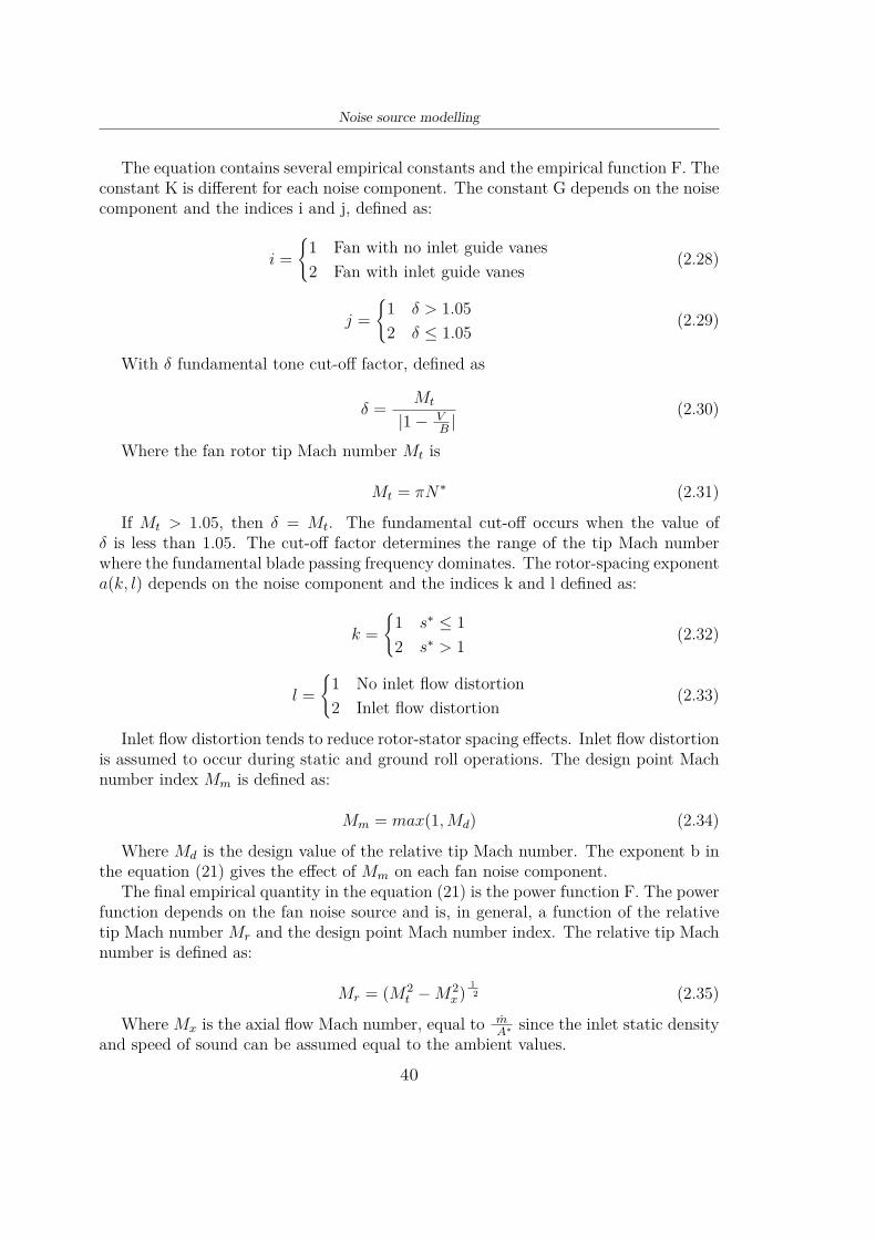
Noise source modelling
The equation contains several empirical constants and the empirical function F. Theconstant K is different for each noise component. The constant G depends on the noisecomponent and the indices i and j, defined as:
i =I
1 Fan with no inlet guide vanes2 Fan with inlet guide vanes
(2.28)
j =I
1 δ > 1.052 δ ≤ 1.05
(2.29)
With δ fundamental tone cut-off factor, defined as
δ = Mt
|1 − VB |
(2.30)
Where the fan rotor tip Mach number Mt is
Mt = πN∗ (2.31)
If Mt > 1.05, then δ = Mt. The fundamental cut-off occurs when the value ofδ is less than 1.05. The cut-off factor determines the range of the tip Mach numberwhere the fundamental blade passing frequency dominates. The rotor-spacing exponenta(k, l) depends on the noise component and the indices k and l defined as:
k =I
1 s∗ ≤ 12 s∗ > 1
(2.32)
l =I
1 No inlet flow distortion2 Inlet flow distortion
(2.33)
Inlet flow distortion tends to reduce rotor-stator spacing effects. Inlet flow distortionis assumed to occur during static and ground roll operations. The design point Machnumber index Mm is defined as:
Mm = max(1, Md) (2.34)
Where Md is the design value of the relative tip Mach number. The exponent b inthe equation (21) gives the effect of Mm on each fan noise component.
The final empirical quantity in the equation (21) is the power function F. The powerfunction depends on the fan noise source and is, in general, a function of the relativetip Mach number Mr and the design point Mach number index. The relative tip Machnumber is defined as:
Mr = (M2t − M2
x)12 (2.35)
Where Mx is the axial flow Mach number, equal to mA∗ since the inlet static density
and speed of sound can be assumed equal to the ambient values.
40
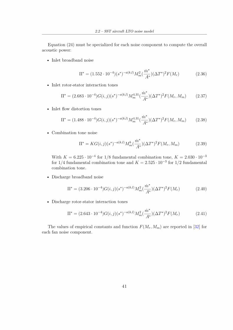
2.2 – SST aircraft LTO noise model
Equation (24) must be specialized for each noise component to compute the overallacoustic power:
• Inlet broadband noise
Π∗ = (1.552 · 10−4)(s∗)−a(k,l)M2m( m∗
A∗ )(∆T ∗)2F (Mr) (2.36)
• Inlet rotor-stator interaction tones
Π∗ = (2.683 · 10−4)G(i, j)(s∗)−a(k,l)M4.31m ( m∗
A∗ )(∆T ∗)2F (Mr, Mm) (2.37)
• Inlet flow distortion tones
Π∗ = (1.488 · 10−4)G(i, j)(s∗)−a(k,l)M4.31m ( m∗
A∗ )(∆T ∗)2F (Mr, Mm) (2.38)
• Combination tone noise
Π∗ = KG(i, j)(s∗)−a(k,l)M bm( m∗
A∗ )(∆T ∗)2F (Mr, Mm) (2.39)
With K = 6.225 · 10−4 for 1/8 fundamental combination tone, K = 2.030 · 10−3
for 1/4 fundamental combination tone and K = 2.525 · 10−3 for 1/2 fundamentalcombination tone.
• Discharge broadband noise
Π∗ = (3.206 · 10−4)G(i, j)(s∗)−a(k,l)M2m( m∗
A∗ )(∆T ∗)2F (Mr) (2.40)
• Discharge rotor-stator interaction tones
Π∗ = (2.643 · 10−4)G(i, j)(s∗)−a(k,l)M2m( m∗
A∗ )(∆T ∗)2F (Mr) (2.41)
The values of empirical constants and function F (Mr, Mm) are reported in [32] foreach fan noise component.
41

Noise source modelling
2.2.3 OutputOnce the distance between the noise source and the observer on ground has been fixed,the semi-empirical equations previously presented allow the computation of the mean-square acoustic pressure for each desired value of frequency, polar directivity angle,and azimuthal directivity angle. Hence, they have been employed in different Matlabroutines to compute the mean-square acoustic pressure of each sub-component of LTOnoise generated by an SST aircraft. After that, the relative Sound Pressure Level(SPL) has been calulated as:
SPL = 10log10 < p2 >∗ +20log10ρ∞c2
∞pref
(2.42)
Where pref is the lowest sound pressure possible to hear to human ear, that isapproximately 20−5 Pa. The final output consists in the Sound Pressure Level (SPL)as a function of frequency for each aircarft noise component. Aircraft position data fornoise prediction and ambient conditions has been fixed to consider a single overflightpoint at the values reported in the Table 2.4. Input data required for each routine arerespectively specified in the following paragraphs.
Noise prediction input dataDistance r 300 mPolar directivity θ 90◦
Azimuthal directivity φ 0◦
Ambient density ρ∞ 1.225 kg/m3
Ambient temperature T∞ 288 KSpeed of sound a∞ 340 m/sMach M∞ 0.23
Table 2.4: Flight path and ambient conditions data.
Airframe noise Directivity functions are provided in Appedix B. Design parametersthat affect noise generation are reported in the Table 2.5. The results obtained showsthat landing gear noise is the most dominant airframe noise source. The clean deltawing does not influence noise generation, whereas vertical tail contribution does notcompare, since for θ = 90◦ its directivity function goes to zero. Ultimatly, looking atreached noise levels, it can be deduced that airframe noise due to supersonic aircraft iscomparable to subsonic airframe noise, and that likely it will not be the most relevantnoise source.
42

2.2 – SST aircraft LTO noise model
Airframe noise parameters
Wing span bw 25.6 mWing surfrace Sw 358.25 m2
Wing span (vertical tail) bv 11.32 mWing surfrace (vertical tail) Sv 33.91 m2
N struct main landing-gear nstrutm 2N wheels main landing-gear nwheelsm 4Tyre diameter main landing-gear dtyrem 1.2 mLength strut main landing-gear lstrutm 2.5 m
N struct forward landing-gear nstrutf 1N wheels forward landing-gear nwheelsf 2Tyre diameter forward landing-gear dtyref 0.787 mLength strut forward landing-gear lstrutf 3 m
Table 2.5: Airframe noise parameters for noise prediction.
Figure 2.8: Airframe noise SPL (θ = 90◦,φ = 0◦).
43

Noise source modelling
Jet noise Jet mixing noise directivity function is provided in Appedix C. The param-eters that affect noise generation are reported in the Table 2.6. Considering a slightlysupersonic jet, the results obtained shows that when shock cells noise occurs, it is theprevalent jet noise source. The main parameters that influence jet noise generationare the exhaust jet speed Vj and the jet Mach number Mj . Hence, jet mixing noisevariation versus Vj and shock cells noise variation versus Mj are reported below. It canbe observed that these contributions icrease with jet exhaust speed and Mach number.
Jet noise parameters
Number of engines Ne 4Engine reference area Ae 1.15 m2
Fully expanded jet area Aj 1.15 m2
Fully expanded jet density ρj 1.225 kg/m3
Jet speed Vj 500 m/sFully expanded jet total temprature Tj 288 KFully expanded jet pressure pj 101325 PaMach Mj 1.05Angle between flight vector and engine inlet axis δ 0◦
Table 2.6: Jet noise parameters for noise prediction.
Figure 2.9: Jet noise SPL (θ = 90◦,φ = 0◦).
44

2.2 – SST aircraft LTO noise model
Figure 2.10: Jet mixing noise SPL versus Vj . Figure 2.11: Shock cells noise SPL versus Mj .
45

Noise source modelling
Fan noise Fan noise directivity function are provided in Appedix C. The parametersthat affect noise generation are reported in the Table 2.7. Observing the Figure 2.11,the main broadband noise contribution is the discharge noise, whereas combinationtone noise causes some peaks in the SPL that depends on the blade passing prequencyfb. The main parameters that influence fan noise generation are the air mass flow m,the rotational speed N and the rise of temperature across fan ∆T . Hence, fan noisevariation versus m, N and ∆T are reported below. It can be deduced that and increasein m and ∆T produces an increment of SPL, whereas N shifts peak values to lowerfrequencies, as it increase.
Fan noise parameters
Number of engines Ne 4Engine reference area Ae 1.15 m2
Fan rotor diameter drot 1.21 mFan reference area Afan 1.15 m2
Number of stator vanes nV 32Number of blades B 19Mean rotor blade chord C 0.22 mRotor-stator spacing s 0.22 mFan rotor relative tip Mach number at design point Md 1Air mass flow m 186 kg/sFan rotational speed N 108 HzTemperature rise across fan ∆T 57.6 K
Inlet guide vane index i 2Flow distorsion index l 1
Table 2.7: Fan noise parameters for noise prediction.
46

2.2 – SST aircraft LTO noise model
Figure 2.12: Fan noise SPL (θ = 90◦,φ = 0◦).
47
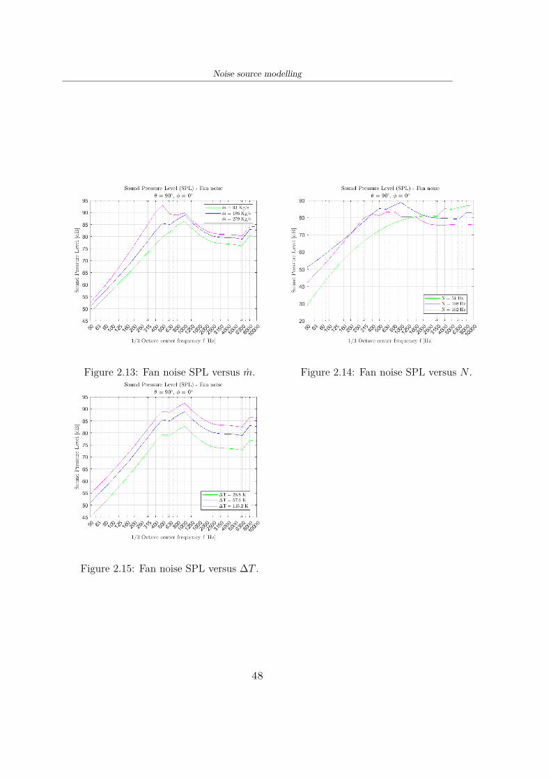
Noise source modelling
Figure 2.13: Fan noise SPL versus m. Figure 2.14: Fan noise SPL versus N .
Figure 2.15: Fan noise SPL versus ∆T .
48

2.2 – SST aircraft LTO noise model
Overall noise Spetrically summing the mean-square acoutisc pressure of each com-ponent and computing the SPL, the overall aircraft noise is predicted. In the Figure2.16 both cases for subsonic and supersonic jet are presented. Generally, airframenoise is not the lowest noise source in comparison with engine noise components. For asubsonic jet flow, jet and fan noise are comparable, whereas, as supersonic conditionsoccurs, the most dominant noise source is jet noise.
Figure 2.16: Overall aircraft noise SPL - subsonic and supersonic jet.
49

50

Chapter 3
Overall methodology
Once the noise model has been defined, it has been inegrated within the overall method-ology in order to predict the ground-based noise level produced by an aircraft movingalong an arbitrary flight path. Hereby, the main properties of the modules interfacingthe noise model are discussed in this chapter. Despite the simple approach, the method-ology includes some of the fundamental aspects for the development of a comprehensivemethod to predict aircraft noise level.
3.1 FrameworkThe overall methodology takes form from the fundamental aircraft noise predictionproblem. The aircraft follows an arbitrary flight path in the presence of an observer onthe ground, that in this case is represented by a microphone placed on the runaway.During this operation, noise sources on the aircraft emit radiation with defined power,directionality, and spectral distribution characteristics, all of which may depend ontime. This source noise propagates through the atmosphere (being attenuated) to thevicinity of the observer. The observer receives signal from the direct ray plus a signalfrom a ray reflected by the local ground surface. Hereby, to develop a methodologyaiming at predicting noise levels generated by an aircraft, different modules differentmodules are required to interface with each other. The way these modules exchangethe information is described in the framework presented in Fig. 3.1.
The framework represents the modular strcuture that underlies the Matlab programbuilt to employ the methodology. The main program calls other routines which loadthe input variables, perform calculations for the various aircraft modules or preparethe output. The main program ecompasses the following sequential steps:
• Definition of the coordinate reference system.
• Entering of data related to airframe/engine design, configuration and operatingcondition of the aircraft along the flight path.
51

Overall methodology
• Selection of the desired trajectory to simulate by user (take-off, landing or simpleflyover).
• Selection of the measurement point on ground where the user wants to predictaircraft noise levels.
• Computation of aircraft noise levels for each sub-components and for overall noisein terms of SPL.
• Processing of the SPL to get noise levels expressed as noise metrics used to quan-tify aircraft noise.
Excluding the first two steps, the others involve the calling for the routines em-ployed to model the components needed to develop a first attempt of a comprehensivemethology to predict aircraft noise levels.
The reference coordinate system is defined as represented in Fig. 3.2, where thereference point for aircraft noise prediction purposes are depicted:
• Sideline noise measurement point: the measurement point is along the line parallelto the axis of runaway centre line at a distance of 450 m, where the noise levelis maximum during take-off. This single point refers to the lateral full-powerreference noise measurement point, even though lateral noise level is typicallymeasured considering a set of ground point along a line placed at a lateral distanceof 450 m from the runaway centre line.
• Flyover noise measurement point: the measurement point is along the extendedrunaway centre line at a distance of 6500 m from the start to roll.
• Approach noise measurement point: the measurement point on the ground is alongthe extended runaway centre line at 2000 m from the threshold. This correspondsto a position 120 m vertically below the 3° descent path originating from a point300 m beyond the threshold.
• Approach threshold: the beginning of approach procedure.
• Start of take-off roll: the beginning of take-off procedure.
• ILS landing point and flight path: the descent path defined for instrumental land-ing, with a descent angle of 3◦.
Once the airspace, the aircraft and the performace along the flight path are defined,the execution of the program allows the user to set the desired trajectory, choosing be-tween take-off, landing or flyover. Then, the simulation of the trajectory runs, callingthe routines of the atmosphere and engine models. The evolution of aircraft configu-ration and operating paramters is continuously update and information about aircraftdistance and noise sources directivity with respect to the microphones on ground arerecorded with a sampling time of 0.5 s. When the simulation ends, the user is enabled
52

3.1 – Framework
Figure 3.1: Overall methodology framework.
53

Overall methodology
Figure 3.2: Coordinate reference system.
to extract the trajectory and the noise measurement point data. Afterwards, the roun-tines, employing the equations of the noise model, compute the mean-square acousticpressure for each contribution and for overall noise for each time instant along theflight trajetory at which the microphone is turned on. Then, the mean-square acousticpressure is converted in the SPL. Ultimatly, the SPL is concurrently processed to getthe A-weighted SPL and the conversion to noisiness levels, to compute respectivelythe OASPL in dBA and the PNL in PNdB over the selected time interval for noisemeasurement. In this way, the LAmax, SEL, PNLTM and EPNL are given as outputof the program.
3.2 Engine modelEngine noise prediction requires specific information about geometry and operationalconditions, so an engine model is needed. Accordingly to the selected case studydescribed in the paragraph 4.1, a two-spool turbojet engine with afterburner has beenmodelled taking as a reference the Olympus 593 MRK 610 (Fig. 3.3) data. Obviously,the type of the engine and the exhasut system affect the noise prediction, thus changingthe case study requires modelling the specific engine under consideration. Furthermore,the equations implemented for the engine modelling must be thought as functionalto the evaluation of the parameters of interest for noise asssessment at a conceptualdesign level. To verify that such a model can also be suitable for off-design studies andperformance analysis is beyond the scope of this work.
The undertaken approach attaining a sufficiently reliable engine model comprisesthe on-design and off-design studies of engine core and the definition of the engineexhaust system. On design and off design conditions have been simulated on the basis
54

3.2 – Engine model
Figure 3.3: Rolls Royce Olympus 593 MRK 610.
of [41], a work that deals with the development and the employment of numericalsimulation technique of stationary and transitional benefits of turbo engines.
Firstly, the engine has been defined without the afterburner, considering the on-design conditions in the Table 3.1.
Figure 3.4: Engine station designation for a two-spool turbojet
The engine stations (Fig. 3.4) are listed below:
• Station 0: Area ahead of the inlet, where the airflow undisturbed.
• Station 1: Inlet diffuser.
• Station 2: Exit inlet diffuser, inlet low pressure compressor.
• Station 25: Exit low pressure compressor, inlet high pressure compressor.
55

Overall methodology
• Station 3: Exit high pressure compressor, inlet combustor.
• Station 4: Exit combustor, inlet high pressure turbine.
• Station 45: Exit high pressure turbine, inlet low pressure turbine.
• Station 5: Exit low pressure turbine, nozzle duct.
• Station 8: Nozzle throat.
• Station 9: Exhaust nozzle.
On designFlight conditionsMach M0 0.7Altitude [m] h 9936.48Specific heat capacity (air) [J/(KgK)] cp 1004Ideal gas constant (air) [J/(KgK)] R 287IntakeAir mass flow [Kg/s] m 186Ram efficiency Ôd 0.98Low pressure compressorLow compressor ratio βcL 3.237Mechanical efficiency ηmcL 1Adiabatic efficiency ηcL 0.87High pressure compressorHigh compressor ratio βcH 4.788Mechanical efficiency ηmcH 1Adiabatic efficiency ηcH 0.87
56
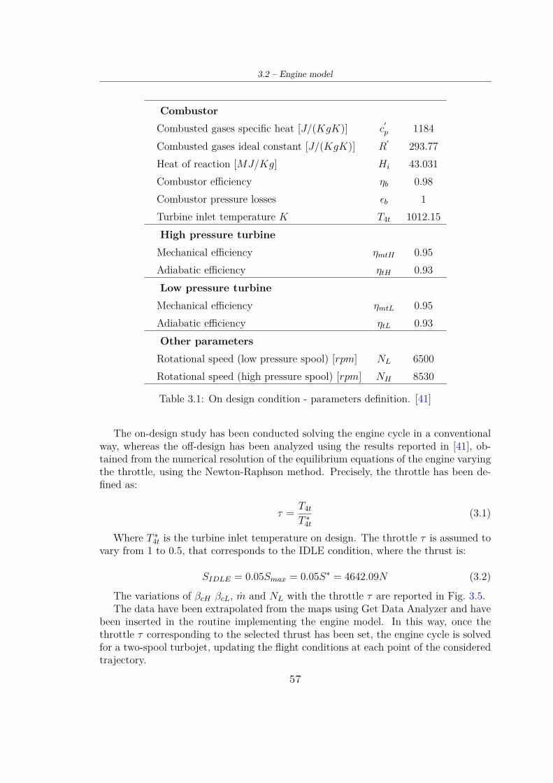
3.2 – Engine model
CombustorCombusted gases specific heat [J/(KgK)] c
Í
p 1184Combusted gases ideal constant [J/(KgK)] R
Í 293.77Heat of reaction [MJ/Kg] Hi 43.031Combustor efficiency ηb 0.98Combustor pressure losses Ôb 1Turbine inlet temperature K T4t 1012.15High pressure turbineMechanical efficiency ηmtH 0.95Adiabatic efficiency ηtH 0.93Low pressure turbineMechanical efficiency ηmtL 0.95Adiabatic efficiency ηtL 0.93Other parametersRotational speed (low pressure spool) [rpm] NL 6500Rotational speed (high pressure spool) [rpm] NH 8530
Table 3.1: On design condition - parameters definition. [41]
The on-design study has been conducted solving the engine cycle in a conventionalway, whereas the off-design has been analyzed using the results reported in [41], ob-tained from the numerical resolution of the equilibrium equations of the engine varyingthe throttle, using the Newton-Raphson method. Precisely, the throttle has been de-fined as:
τ = T4t
T ∗4t
(3.1)
Where T ∗4t is the turbine inlet temperature on design. The throttle τ is assumed to
vary from 1 to 0.5, that corresponds to the IDLE condition, where the thrust is:
SIDLE = 0.05Smax = 0.05S∗ = 4642.09N (3.2)
The variations of βcH βcL, m and NL with the throttle τ are reported in Fig. 3.5.The data have been extrapolated from the maps using Get Data Analyzer and have
been inserted in the routine implementing the engine model. In this way, once thethrottle τ corresponding to the selected thrust has been set, the engine cycle is solvedfor a two-spool turbojet, updating the flight conditions at each point of the consideredtrajectory.
57

Overall methodology
Figure 3.5: Engine parameters versus throttle τ at equilibrium.[41]
58

3.2 – Engine model
The afterburner has been modelled by the addition of another component after thelow pressure turbine, that gives in exit a flow reaching a total temperature of 1700K, considering an afterburner efficiency of 0.9. Precisely, since no data are availableabout aftererburners mounted on SST aircraft, the value of the afterburner exit totaltemperature has been selected from the General Electric J85, a one-spool turbojet eithafterburner [41]. At least, an exhaust system aiming at predicting the exhaust jetparameters as a function of thrust has been modelled. The Olympus 593 was equippedwith an exhaust assembly comprises of a variable exhaust with a primary nozzle anda secondary nozzle. The primary nozzle sits at the end of the jet-pipe, and is a ringof petals operating in unison to vary the diameter, and therefore then the area of thejet pipe exit. The secondary nozzle assembly surrounds the primary nozzle; it was anarrangement of hinged buckets, whose position can be varied to control the exhaustin the most efficient way during all stages of flight Fig. 3.6. Together they make upanother form of convergent/divergent duct.
Figure 3.6: Modulation of twin secondary nozzle exhaust area.
For the applications of this work, the nozzle has been considered as a convergentnozzle with variable area, whereas the exhaust system has been assumed to be a di-vergent ejector nozzle, with an exhaust area (equal to fully expanded jet area) that isthe 20 % larger than the throath area. Precisely, the ratio of the exit and throat areahas been found in [42], between a range of typical values. Finally, the hypothesis madeare:
• Isentropic and adiabatic flow, since no shock waves occur within the conver-gent/divergent duct.
59
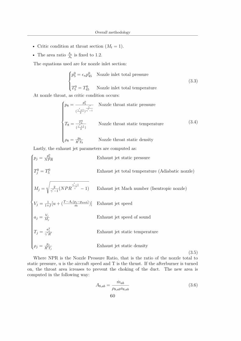
Overall methodology
• Critic condition at throat section (Mt = 1).
• The area ratio AeAt
is fixed to 1.2.
The equations used are for nozzle inlet section:p0
5 = Ônp045 Nozzle inlet total pressure
T 05 = T 0
45 Nozzle inlet total temperature(3.3)
At nozzle throat, as critic condition occurs:
p8 = p05
( γÍ +12 )
γÍ
γÍ −1
Nozzle throat static pressure
T8 = T 05
( γÍ +12 )
Nozzle throat static temperature
ρ8 = p8RÍT8
Nozzle throat static density
(3.4)
Lastly, the exhaust jet parameters are computed as:
pj = p05
NPR Exhaust jet static pressure
T 0j = T 0
5 Exhaust jet total temperature (Adiabatic nozzle)
Mj =
ó2
γÍ −1(NPRγ
Í −1γ
Í − 1) Exhaust jet Mach number (Isentropic nozzle)
Vj = 11+f [u + (T−Ae(pj−pamb)
m )] Exhaust jet speed
aj = VjMj
Exhaust jet speed of sound
Tj = a2j
γÍRÍ Exhaust jet static temperature
ρj = pjRÍTj
Exhaust jet static density(3.5)
Where NPR is the Nozzle Pressure Ratio, that is the ratio of the nozzle total tostatic pressure, u is the aircraft speed and T is the thrust. If the afterburner is turnedon, the throat area icreases to prevent the choking of the duct. The new area iscomputed in the following way:
A8,ab = mab
ρ8,aba8,ab(3.6)
60

3.3 – Trajectory simulation
Where mab is the sum of air and fuel mass flow, ρt,ab is the density at the throatand at,ab is the flow speed at the throat. These values take into account the increaseof total temperature due to the afterburner:
p8,ab = p05,ab
( γÍ +12 )
γÍ
γÍ −1
Nozzle throat static pressure
T8,ab = T 05,ab
( γÍ +12 )
Nozzle throat static temperature
ρ8,ab = p8,abRÍT8,ab
Nozzle throat static density
ρ8,ab = p8,abRÍT8,ab
Nozzle throat static density
(3.7)
Where: p0
5,ab = Ôabp045,ab Afterburner exit total pressure
T 05,ab = 1700K Afterburner exit total temperature
(3.8)
Where Ôab is equal to 0.9 and indicates the afterburner pressure losses.
3.3 Trajectory simulationUsually, to predict ground noise immission along a flight path, the corresponding tra-jectory is assembled from straight flight segments with constant operational and con-figurational setting. Accordingly to this approach, the take-off and landing trajectoryhas been simulated as a flight path composed respectively by 5 and 3 flight segmentconstructed from fixed point data defining constant speed, thrust and altitude. How-ever, an update of speed and thrust has been included, in order to gain a more accurateprediction of noise levels. Then, during the aircraft overflight, the measurement dataare detected for a given interval of time at the three certification measurement pointsdefined by ICAO. In the Figure Fig. 3.7 the input and the output of the routinesimplemented to simulate the LTO trajectories are reported.
Once the operational procedure data have been set and engine data have beendefined, the routine updates aircraft position and performance data, including thecomputation of ambient conditions considering the standard atmosphere model. Theoutuput comprises of flight conditions, noise measurement point data for each noisemeasurement point, jet noise and fan noise data. These information are known for eachpoint of the flight path and when the user select the point where he wants to predictaircraft noise level, the program extracts ambient conditions and noise measurementdata relative to that point.
61

Overall methodology
Figure 3.7
3.4 Noise metricsSound is the result of a sound source inducing vibration in the air. The movementof the particles causes fluctuations in the normal atmospheric pressure, that producessound waves. These waves radiate in all directions from the source and may be reflectedand scattered or may turn corners. When the source stops vibrating, the sound wavesdisappear almost instantaneously, and the sound ceases. This physical phenomena maybe described in terms of frequency, amplitude and time pattern.
The rate at which a sound source vibrates, or makes the air vibrate, determinesfrequency, that is measured in Hz. In real-life situations, it is rare to found a soundcharacterized by a single frequency (a pure tone). Most of the sounds consist insteadof a complex mixture of many frequencies. The frequency content of these sounds ischaracterized by a band of frequencies, usually an octave or 1/3 octave in width. Soundpressure is the amplitude or measure of the difference between atmospheric pressure(with no sound present) and the total pressure (with sound present) and its unit is thedB, that is expressed in a logarithmic scale, as in this way it is possible to encompassall the wide range of sound intensities. Such aspect means that the sound pressurelevels of two separate sounds are not directly arithmetically additive. For example,if a sound is added to another sound of equal intensity, the total is only a 3 decibelincrease or if the added sound is less to the higher of 10 dB or more, it does not affectthe higher level.Lastly, the time pattern describes the temporal nature of the soundproduction, and it may be continuous, intermittent, impulsive or fluctuating.
Acoustic noise is classified as an unwanted sound considered unpleasant, loud ordisruptive which is audible to the human ear. Such a particular sound can be quantifyby a noise metric, that is an expression used to describe any measure of quantity of
62

3.4 – Noise metrics
noise at a receiver position. To assess the loudness or the annoyance of aircraft noiseon human hearing system, a number of noise metrics are in using among differentaviation organization, countries and airports [43]. However, aircraft noise metrics canbe classified into three groups of measurement types [44]:
• Single event (or instantaneous) metrics: measurements taken to describe the noiseoccurring during one noise event, accounting only for sound amplitude. It istypically expressed as the maximum sound level reached during the event.
• Exposure (or intergral) metrics: used to provide a description of the type of noiseexposure experienced over a given period of time. It is computed as a integralover a defined time interval.
• Supplementary metrics: measurements often used in conjunction with the above,to provide a more meaningful depiction of the potential impact of noise exposure.
The loudness of a noise emission is directly linked to the quantity of energy trans-ferred throught the air causing changes in air pressure. The more energy put intomaking a sound, the louder it will be. Hence, the different noise metrics rely on differ-ent methods to evaluate the energy of a noise event, as previously described.
Aircarft noise metrics commonly in using are typically single event and exposuremetrics. The instantaneous sound level metric can be frequency weighted or computed.The weighted sound level results from the correction of SPL, modified to de-emphasizethe low frequency portion of sounds to approximate the human ear’s response to sound.Once the frequency weighted Overall Sound Pressure Level (OASPL) evolution isknown over a certain period of time, the instantaneous sound level corresponds tothe maximum sound level recorded. There are several weightings (A, B, C, D) foundon a sound level meter, but A-weighting is the most widely used by federal, state, andlocal agencies for environmental noise analyses to approximate the relative noisiness orannoyance of many commonly occurring steady state or intermittent sound. The noisemetric associated with this A-weighted SPL is indicated as LAmax and is measured indBA. Its graphical representation is given in Fig. 3.8.
The computed instantaneous noise metric used to measure aircraft noise is thePerceived Noise Level (PNL), that is a rating of the noisiness of a sound calculated fromacoustic measurements. It is computed from sound pressure levels typically measuredin one-third octave frequency bands and it is expressed in terms of PNdB. The PNLof a given sound is intended to be numerically equal to the level of an octave band ofnoise centered at 1000 Hz, which is judged equally noisy to the given sound [53]. Thenoise level associated with this metric is the Maximum Tone Corrected PercedivedNoise Level PNLTM. The procedure used to derive the PNLTM from experimentalmeasurements is standardized by ICAO in [12], and involves spectral analysis, withthe conversion of SPL in noisiness levels by means of the correspondence with noytables associated with each value of SPL for a given frequency and correction forspectral irregularities. Having the Tone Corrected Perceived Noise Level (PNLT) timeevolution, the PNLTM is computed in the same manner as the LAmax, identifying themaximum sound level recorded.
63

Overall methodology
Figure 3.8: Graphical representation of LAmax. [44]
The integral noise metrics are duration corrected single event metrics. Hence, SoundExposure Level (SEL) is energy averaged A-weighted sound level over a specified pe-riod of time or single event, with a reference duration of 1 second. On the other hand,Effective Perceived Noise Level (EPNL) consists of an integration over the noise dura-tion of the PNLT, normalized to a reference duration of 10 s and measured in EPNdB.Both of these integral metrics require the definition of the time interval for integra-tion, which is identify by the first and the last instant of time (kF and kL) when thesound level is 10 dBA or PNdB respectively lower than the maximum level. Graphicalrepresentation for SEL is presented in Fig. 3.9.
All the described metrics are used for aircraft noise certification. Precisely, LAmax
and SEL are considered as loudness-based metrics, whereas PNLTM and EPNL areannoyance-based. It is also possible to find some approximated relationships bewteenboth instantaneous and integral noise metrics. Altough the different ways of process-ing the frequency distribution of energy, in practice there is a fairly high correlationbetween the LAmax and PNLTM measures, that is PNLTM Ä LAmax + 13. How-ever the exact correction figure depends on factors such as aircraft type, operationalcharacteristics, meteorological conditions and the distance from the aircraft flight path[44]. For exposure noise metrics, the rationale for normalising EPNL to 10 secondsis to penalise those aircraft that make a lot of noise for a relatively long time. As aconsequence, the EPNL imparts greater subjective emphasis to energy at frequenciesabove 1 kHz and applies a tone correction, or ‘penalty’, in proportion to the protrusionof any discrete frequencies above the adjacent 1/3 octave band levels, whith resepct to
64

3.4 – Noise metrics
Figure 3.9: Graphical representation of SEL. [44]
SEL. Such tone correction in EPNL was originally introduced because early jet aircraftengines generated extremely high (and therefore annoying) fan and turbine tone levels.SEL were not thought to fully reflect these annoying tone levels. However, for modernengines, the corrections tend to be zero or small so that, although EPNL values remainnumerically larger (about 3 or 5 dB) than SEL, the differences are fairly consistentacross a wide range of current aircraft types [44].
Whitin the developed methodology, all the cited noise metrics have been computedfrom the SPL given in output by the routines dedicated to the noise source modelling.The procedure adopted is schematized in the diagram presented in Fig. 3.10.
First of all, it is needed to consider the attenuation of sound due to atmosphericabsorption, since the distances between the noise source and the observer consideredunder the scope of this thesis are such that sound attenuation in the atmosphere is not anegligible phenomena. When a noise source emits sound waves, the observer on ground,placed at a certain distance from the source, receives a sound being attenuated for anumber of factors which influence the propagation of noise. However, temperature andhumidity are the parameters causing major reduction in sound as distance increasing.To determine the entity of these lossess, the mathematical procedure suggested in SAEARP 866 B [54] has been adopted. The SARP considers only the classical and molecularabsorption of sound energy by the atmosphere. The classical absorption results fromenergy dissipation through the effects of heat conduction and viscosity and is a functionof frequency and temperature, whereas molecular absorption results principally from
65

Overall methodology
Figure 3.10: Procedure adopted in the overall methodology to compute noise metrics.
rotational and vibrational relaxion process of oxygen and nitrogen molecules and is afunction of frequency, temperature and humidity. In particular, classical absorptionis important only at higer frequencies and varies slightly with temperature; molecularabsorption is the main contribution to sound attenuation, varying on a wide range ofvalues, producing an higher sound reduction at highest frequencies. The SAE ARP866 B reports a seven-step procedure that leads to the total atmospheric absorptioncoefficients as a sum of classical absorption component and a molecular absorptioncomponent. The total loss is expressed as the attenuation in db/100 m and is a functionof frequency, temperature and relative humidity, defined as the amount of water vapourpresent in air expressed as a percentage of the amount needed for saturation at sameair temperature. As a result, summing algebrically the lossess for each centre frequencyin 1/3 octave band of the spcectrum, the SPL receveid on ground is obtained.
This SPL is a function of frequency and time. Another step is required beforethe calculation of the noise metrics. To get the LAmax and SEL, A-weighting ofthe frequency spectrum is needed. The new SPL is computed summing algebricallytabulated coefficients that de-emphasize the low frequency portion of sounds for each1/3 octave centre frequency. Once the A-weighted SPL is given, it is possible tocompute the OASPL, that is just a function of time, with the following formula:
OASPL(k) = 10log10
24Øi=1
10(SPLA(i,k)/10) (3.9)
Where i indicates the 1/3 frequency band considered between 50 Hz and 10000 Hz.Computing the OASPL for each time-instant k, the sound pressure level time evolutionis known. Hence, the LAmax is simply obtained as:
LAmax = max(OASPL(k)) (3.10)
The OASPL is defined over a certian time intervall with a sampling time of 0.5 s.
66

3.4 – Noise metrics
In order to obtain the information about the time instant kF and kL, when the soundlevel reaches the value LAmax − 10 dBA, the OASPL is interpolated and then kF andkL are determined with a tolerance of 0.1 dBA. At least, the SEL is computed as:
SEL = 10log10
kLØk=kF
10(OASPL(k)/10) (3.11)
The calculation of PNLTM and EPNL is quite similiar to the one just exposed.Firstly, PNL(k) is calculated from instantaneous 1/3 octave band sound levels, SPL(i,k),accordingly to the procedure described in [12]. Precisely, three steps have to be per-formed:
• Conversion of each 1/3 octave band SPL(i,k) from 50 to 10000 Hz to perceivednoisiness n(i,k).
• Combine the perceived noisiness values n(i,k) in the following formula:
N(k) = 0.85n(k) + 0.1524Øi=1
n(i, k) (3.12)
Where n(k) is the largest of the 24 values of n(i,k) and N(k) is the total perceivednoisiness.
• Convert the total perceived noisiness, N(k), into PNL(k), by the following formula:
PNL(k) = 40 + 10log102 log10N(k) (3.13)
After that, spectral irregularities are adjusted by the correction factor C(k), cal-culted on the basis of the evaluation of the slopes in SPL spectrum. Finally, the PNLTis computed as:
PNLT (k) = PNL(k) + C(k) (3.14)
Therefore, the PNLTM is defined as:
PNLTM = max(PNLT (k)) (3.15)
Once the time instant kF and kL are determined, the EPNL can be calculatedconsidering a sampling time of 0.5 s and a reference noise duration of 10 s:
EPNL = 10log10
kLØk=kF
10(PNLT (k)/10) − 13 (3.16)
Where 13 dB is a constant relating the one-half second values of PNLT(k) to the10 s reference duration.
67

68

Chapter 4
Validation
After a description of the selected case study and the reference database, the Chapterprovides the results derived from the matching between the experimental NPD curvesand the predicted NPD curves. Thus, the accuracy of the developed methodology inpredicting the overall aircraft noise level has been estimated for flyover trajectories atdifferent altitudes and thrust ratings.
4.1 Case studyConcorde was a supersonic civil transport category aircraft capable of carrying aprox-imatly 100 to 125 passengers over extended routes at a cruising speed that is 2.5 timesgreater than that of subsonic aircraft.
Although the intention of this work is turned towards the next generation of SSTaircraft, it is conceivable to assume the Concorde design as an initial reference, as itincludes the main characteristics of an SST aircraft (Fig. 4.1).
Concorde has an ogival delta planform wing, with thickness/chord ratio 3% at root,2.15% from nacelle outboard. Longitudinal and lateral control was provided throughthree elevons on trailing-edge of each wing, of aluminium alloy honeycomb construction.Each elevon is independently operated by a tandem jack, each half supplied from anindependent hydraulic source and controlled by a separate electrical system; therewere not higli-lift devices, while leading-edges ahead of air intakes are electrically de-iced. Directional control was provide through vertical fin and rudder only; two-sectionalluminium rudder controlled in same way as elevons. Another typical feature of theConcorde was the droop nose: precisely, nose was drooped hydraulically to improveforward view during take-off, initial climb, approach and landing. Retractable visorwas raised hydraulically to fair in windscreen in cruising flight. Landing gear washydraulically-retractable tricycle type; twin-wheel steerable nose unit retracts forwardand our-wheel bogie main units retract inward. It was provided with oleo-pneumaticshock-absorbers and retractable tail bumper. About the powerplant, Concorde wasa four-jet supersonic transport. The engine was the Rolls-Royce/Snecma Olympus593, a two-spool turbojet with afterburner, initially designed for military aircraft and
69

Validation
Figure 4.1: Concorde views.
later adapted for civil applications. Each engine consisted of hydraulically controlledvariable-area (by ramp) air intake, engine bay and nozzle support structure. Fuelsystem was used also as heat sink and to maintain aircraft trim. Indeed, all tankswere of integral construction and were in two groups, with total usable capacity ofabout 117285 litres. In particular, main group included five tanks in each wing andfour tanks in fuselage and maintains CG automatically in cruising flight, maintainingcorrect relationship between CG and aerodynamic centre of pressure by transferringfuel rearward during acceleration and forward during return to subsonic flight.
Finally, another peculiarity of the Concorde and in general of the SST aircraftsis the mission profile. Concorde flew on fixed and dedicated east-west ocean routesover the North Atlantic Ocean. These routes and the relative heights were definedin such a way as to avoid interference with subsonic air traffic. The cruising altitudeis between FL500 and FL600, as at that altitude changes in weather conditions havesuch a low influence that no change of route is necessary. The take-off took placewith the afterburner on in order to reach the speed required for rotation and lift off.The afterburner was also used to reach the supersonic phase of the cruise. During theflight phases over continental areas supersonic flight was not allowed for aero-acousticreasons, so the aircraft was forced to maintain a Mach of 0.93-0.95. Until supersonicflight was allowed, the Concorde was forced to maintain a constant flight altitude; forexample, New York Air Control directed the aircraft toward the ocean at an altitudeof FL300 before authorizing acceleration to cruising speed. The phases of ascent andacceleration from subsonic to supersonic were the most critical from the point of viewof the aircraft wall temperature. Given the criticality of the acceleration phase, the
70

4.1 – Case study
Concorde needed a free corridor from the point where the afterburners were turnedon to the point where they were turned off (phase no longer than 15 minutes). Thefact that the cruising altitude is defined between FL500 and FL600 is due to the factthat the aircraft was on a parabolic trajectory and not at a fixed altitude to minimizeskin temperatures. When the temperature reached 127 °C the autopilot performed atemperature-dependent trajectory and no longer Mach-dependent. The descent phase,in analogy to the climb phase, starts with a supersonic descent to FL410, until thesubsonic transition, another critical phase that can generate shock waves, therefore itmust not take place near populated areas. The choice of FL410 is given by the factof not wanting to have excessive losses in terms of performance and fuel consumption.When landing, once the touchdown has been made, the minimum runway length hadto be 1830 m [49].
In the Tables A.2, 4.2, 4.3, 4.4 and 4.5 are listed the reference data collected from[47] and [48]. The data refer to the initial production version Concorde Series 200, ofwhich the flrst two examples were flown on 6 December 1973 at Toulouse (F-WTSB)and 13 February 1974 at Filton (G-BBDG).
In conclusion, the Concorde and SST aircraft feautures that affect LTO noise gen-eration are:
• For the airframe noise: the wing planform, the control surfaces and the landinggear. In particular, due to a limited effectiveness of the horizontal tail plane, thearchitecture with elevons is preferred for controlling supersonic aircrafts, whichwill be devoid of the horizontal tail plane. On the other hand, the landing geartypically has a tricycle architecture with longer legs than those of supersonicaircraft, to allow take off at high angles of attack. Precisely for the latter reason,the Concorde has not the secondary control surfaces, which would therefore havebeen aerodianamically inefficient.
• For the engine noise: the type of engine and its operational parameters. Typicallytoday supersonic aircrafts are propelled with turbofan engines with afterburner.Such a powerplant manly contributes to the noise generation during take-off andis the reason why the noise level of a supersonic aircraft is greater with respect tosubsonic one.
71

Validation
Airframe
Delta wing Wing span bw [m] 25.56Surface Sw [m2] 358.25Aspect Ratio AR 1.7Root chord cr [m] 27.66Sweep angle Λ [°] 55Elevons area Selev [m2] 32
Vertical tail Height bv [m] 11.32Surface Sv [m2] 33.91Root chord cv [m] 10.59Rudder area Srudd [m2] 10.40
Landing gear N structure (main) 2N wheels (main) 4Tyre diameter (main) dtyrem [m] 1.2Structure length (main) lstructm [m] 2.5
N structure (forward) 1N wheels (forward) 2Tyre diameter (forward) dtyref [m] 0.787Structure length (forward) lstructf [m] 3
Fuselage Length (overall) lf [m] 61.66Width (max) dmax [m] 2.88Heigt (max) hmax [m] 3.32
Table 4.1: Concorde reference airframe data
72

4.1 – Case study
Engine
General characteristics Number 4Type Turbojet
(Rolls-Royce/SnecmaOlympus 593)
Length leng [m] 4.039Diameter deng [m] 1.212
Components Compressor Axial-flow(7 stages high-pressure,7 stages low-pressure)
Combustors Nickel alloy constructionannular chamber
Turbine 2 stages(1 stage high-pressure,1 stage low-pressure)
Fuel type Jet A-1
Performance Max Thrust [kN ] wet: 169.2, dry: 139.4Overall pressure ratio 15.5Air mass flow [Kg/s] 186SFC (cruise) [g/(kN ∗ s)] 33.8
Table 4.2: Concorde reference engine data
Weights and loadings
Operating Empty Weight OEW [Kg] 78015
Maximum Take-off Weight MTOW [Kg] 176445
Max Zero-Fuel Weight MZFW [Kg] 92080
Max Landing weight MLW [Kg] 78015
Max Wing Loading W/S [Kg/m2] 488
Thrust - to - Weight ratio T/W 0.373
Table 4.3: Concorde reference weights and loadings
73

Validation
Performance
Max Cruising Speed (15635 m) Vcruise [m/s] 272.656
M = 2.05
Rate of climb at S/L Vv [m/min] 1.525
Service ceiling h [m] 18290
Take-off distance [m] 3124
Landing distance [m] 2444
Range with max fuel and 5352 Kg payload [m] 7215
Range with max payload at M = 2.05 [m] 6380
Table 4.4: Concorde reference performance
Operational noise characteristics
Sideline reference EPNLL [EPNdB] 111
Cutback reference EPNLF [EPNdB] 114
Approach reference EPNLA [EPNdB] 115
Table 4.5: Concorde reference operational noise characteristics
74

4.2 – ANP database
4.2 ANP databaseThe ANP database is an online data resource makes available by Eurocontrol Exper-imental Cente to accompain the ECAC Doc 29 and ICAO Doc 9911 guidance docu-ments on airport noise contour modelling [50]. The collected data are related to engineand aerodynamic coefficients and weights for take-off and landing at reference ambi-ent conditions (mean sea level elevation and 15◦C for air temperature) and providealso default procedural steps to enable the construction of flight profiles. To supportthe computation of noise contours around airports, the database comprises also NoisePower Distance (NPD) and Spectral classes data. Having this set of information, theprocedure described in [51] enables the evaluation of ground-noise around the airport.
For noise modelling purposes, the three-dimensional flight path has to be con-structed through the synthesis of different segments or procedural steps that describethe pilot’s selections of engine power, flap angle, and acceleration/vertical speed. Thedifferent kinds of segments reported in ANP are take-off ground roll, climb at constantspeed, power cutback, accelerating climb and flap retraction, accelerating climb afterflap retraction, descent and deceleration and final landing approach.
Once aircraft movements are identified throught the segmentation of the trajec-tory, the geometrical aspects of sound radiation and propagation between aircraft andobserver are determined. This process allows the computation of noise levels, bothmaximum and time integrated, from NPD data, that define noise from aircraft travers-ing idealised horizontal flight paths of infinite length at constant speed and power atreference ambient conditions. The noise contributions from each of these segments aresubsequently summed at the observer position.
NPD curves NPD relatonships are noise event levels tabulated as a function ofdistance below an aeroplane in steady level flight at a reference speed (V = 160 knots),in a reference atmosphere, for each of a number of engine power settings. The dataaccount for the effects of sound attenuation due to spherical wave spreading (inverse-square law) and atmospheric absorption. The distance is defined perpendicular to theaeroplane flight path and the aircraft wing-axis (i.e. vertically below the aircraft innon-banked flight) [51]. Noise levels are typically expressed in terms of LAmax andSEL and depends on specific aircraft types, variants, flight configurations (approach,departure, flap settings) and power settings.
Maximum noise level and time integrated (applicable to an infinite flight path)are generaly estimated by an interpolation, unless values happen to be tabulated forpower-setting and/or distance exactly. A linear interpolation is used between tabulatedpower-settings, whereas a logarithmic interpolation is used between tabulated distances(Fig. 4.2). If Pi and Pi+1 are engine power values for which noise level versus distancedata are tabulated, the noise level L(P ) at a given distance for intermediate power P ,between Pi and Pi+1, is given by:
L(P ) = L(Pi) + L(Pi+1) − L(Pi)Pi+1 − Pi
(P − Pi) (4.1)
75

Validation
If, at any power setting, di and di+1 are distances for which noise data are tabulated,the noise level L(d) for an intermediate distance d, between di and di+1 is given by:
L(d) = L(di) + L(di+1) − L(di)log(di+1) − log(di)
(log(d) − log(di)) (4.2)
By using these equations a noise level L(P, d)) can be obtained for any power settingP and any distance d that is within the envelope of the NPD data base, where theenvelope is defined by air temperature less than 30◦, product of air temperature andrelative humidity greater than 500 and wind speed less than 8 m/s.
Figure 4.2: Interpolation in NPD curves [51].
For distance d outside the envelope, data are extrapolated on the basis of the samelinear interpolation equations, with a lower limit of 30 m be imposed on d, as, at shortdistances, noise levels increase very rapidly with decreasing propagation distance.
4.3 ResultsThe Matlab routines have been employed to get the NPD curves for the selected casestudy. Once the input data have been fixed, a series of flyover trajectories at differentaltitudes and power settings with constant aircraft speed has been simulated within areference airspace, considering a distance on ground long 10 Km and a time intervalfor noise measurement of 120 s ((Fig. 4.3)). In this way, using a linear interpolationfor the results obtained for each pair of altitude and thrust, it was possible to obtainthe NPD curves for the considered aircraft for each power setting.
Hence, the accuracy of the developed methodology has been evaluated by the com-parison of the NPD curves from ANP database and the predicted NPD curves, for bothsingle event and time integrated noise metric, i.e. LAmax and SEL.
Input data for simulation are reported in the Tables 4.6, 4.7 and 4.8.
76

4.3 – Results
Aircraft speed V 82 m/sAmbient temperature T 15◦CRelative humidity HR 0.7
Table 4.6: Aircraft speed and ambient conditions.
Altitude[ft] [m]630 1921000 3052000 6104000 12196300 192010000 3048
Table 4.7: Altitude variations.
Thrust[lb] [N ]
10000 4448020000 8896028000 12455032000 142340
Table 4.8: Thrust variations.
77

Validation
The aircraft speed has been fixed at V = 80 m/s in accordance with the referenceairspeed used to derive the NPD curves from experimental measurements, whereas theambient conditions have been set to the reference conditions suggested in [51] for noisecontours modelling around the airports.
The NPD curves reported in the ANP database are defined for a range of altitudesthat varies from 200 ft (61 m) to 25000 ft (7620 m). Since the noise levels cannot bemeasured experimentally, the values at higher altitudes are typically obtained by theextrapolation of the measured data and may be less accurate. Therefore, accountingalso for the limitations of the semi-empirical methods for lowest and highest altitudes,it was considered conceivable to exclude them and perform the validation for altitudesthat varies from 630 ft (192 m) to 10000 ft (3048 m) for each power setting.
Figure 4.3: Airspace for validation.
The airspace has been defined to correctly predict the SEL, as a time integrated noisemetric calculation need the identification of the two time instants in which the OASPLis 10 dBA less than the maximum. If the time interval for noise measurement is tooshorter, the microphone will not detect the noise levels at 10 dBA less than maximum.So, a reasonable time interval of 120 s has been fixed. Consequently the distance onground, that follows the x-axis track of the aircraft, has to be at least of 9840 Km,that is the distance that an aircraft runs at 82 m/s in 120 s. The microphone is placedat the middle of the runaway and turned on for the fixed time interval, detecting theaircraft movements paramaters that are necessary to compute the noise levels. TheLAmax is the maximum A-weighted sound level recorded during the over-flight of theaircraft, considering each time instant in which the microphone is turned on. The SELrepresents the entire noise event uniformly compressed into a reference time of onesecond, hence it is computed as the sum of sound pressure contained within the timeinterval between kF and kL, that are the two time instants at which the OASPL is10 dBA less than the maximum. As the time interval defined to record the sound isnot enough to detect the SEL at higher altitudes, if kF and kL are not identified, SEL
78

4.3 – Results
is computed with the empirical formula contained in INM Handbook [52], used as astandard procedure to derivate NPD curves by the extrapolation of measured data:
SEL = LAmax + 7.19 + 7.73log10(D/1000) (4.3)
Where D is the distance from ground in ft.
Figure 4.4: Matching with NPD curves - LAmax
Figure 4.5: Matching with NPD curves - SEL
79

Validation
The prediction error has been calculated in absolute terms respectively for LAmax
and SEL as:
ELAmax = LAmaxp − LAmaxANP (4.4)
ESEL = SELp − SELANP (4.5)
Where LAmaxp and SELp are the predicted noise levels. Ultimatly, the RMSE hasbeen computed as:
RMSELAmax =i=NØi=1
ó(LAmaxp(i) − LAmaxANP (i))2
N(4.6)
RMSESEL =i=NØi=1
ó(SELp(i) − SELANP (i))2
N(4.7)
Where N is the number of noise levels considered for each thrust rating varying thealtitude. The matchings between the predicted and the experimental values for thenoise metrics under consideration are presented in Fig. 4.4 and Fig. 4.5 and the resultsare tabulated in 4.9 and 4.10. Analyzing the results for LAmax, the prediction error isbetween −1.51 dBA and 1.38 dBA, whereas for SEL is between −1.55 dBA and 1.52dBA. Looking at LAmax, the method seems to underpredict the maximum noise levelat the lowest thrust rating. On the contrary, the SEL is overpredicted by the methodfor the lowest thrust rating. However, looking at the resultas for all power settings,some correlation cannot be found between the accuracy of the method and the thrustratings.
Error [dBA] - LAmax T = 44480 N T = 88960 N T = 124550 N T = 142340 Nh = 192 m -0.78 0.60 -0.64 -0.54h = 305 m -0.65 0.14 0.07 0.31h = 610 m -0.46 0.62 0.83 1.08h = 1219 m -0.54 0.69 0.99 1.38h = 1920 m -0.78 0.41 0.77 1.18h = 3048 m -1.51 -0.67 -0.23 0.23
Error [dBA] - SEL T = 44480 N T = 88960 N T = 124550 N T = 142340 Nh = 192 m 0.90 -1.17 -1.55 -1.51h = 305 m 1.19 -0.29 -0.60 -0.35h = 610 m 1.43 0.53 0.42 0.79h = 1219 m 1.52 0.79 0.89 1.35h = 1920 m 1.25 0.64 0.76 1.21h = 3048 m 0.43 -0.31 -0.10 0.36
Table 4.9: Prediction error - LAmax and SEL.
80

4.3 – Results
RMSE [dBA] - LAmax
T = 44480 N T = 88960 N T = 124550 N T = 142340 N0.86 0.55 0.67 0.90
RMSE [dBA] - SELT = 44480 N T = 88960 N T = 124550 N T = 142340 N
1.18 0.69 0.88 1.03
Table 4.10: RMSE - LAmax and SEL.
Rather it is possible to ascertain that the prediction error become greater at lowestaltitudes, and has been verified that this situation occurs also for altitudes higherthan the ones considered. These discrepancies are discussed also in [53], where themotivation is attributed to the sound attenuation for atmospheric absorption basedon distance, temperature and relative humidity. Precisely, the document deals withan investigation about significant anomalies with measured and theoretical results inderiving NPD curves to be used in INM. To determine the NPD curve, one needsto extract the atmospheric and distance attenuation components to provide a sourcelevel, move the aircraft to a new position and then apply the distance attenuation andatmospheric attenuation for a reference atmosphere of 25◦C, 101325 Pa and relativehumidity of 70%. By that method one could validate the NPD curve for any positionand any atmospheric conditions. However, when seeking to verify the results with thefield measurements, agreement could not be obtained between the field measurementsand the predicted levels for smaller and larger distances, as depicted in the Fig. 4.6.
The INM is based on the algorithm and framework from the SAE AIR 1845 stan-dard, which considers SAE ARP 866 B for atmospheric absorption coefficient calcu-lation. Since in this validation a temperature of 15◦C has been considered, typicallyan overstimation of noise levels occurs for altitude between 300 m and 1920 m, ratherthan an undestimation that could occur with a temperature of 25◦C. However, thetrend is similalr to NPD curve derived following the SAE AIR 1845 standard.
Ultimatly, the prediction error falls within [-1.55, 1.52] dBA for both the noise met-rics considered, with a more accurate prediction for single event metric. The NPDcurve trend typically undestimate the noise level for lowest and highest altitude, andslightly overstimate the middle altitudes. Probably, changing the reference ambientconditions, the method could gain an higher accuracy for the middle altitudes. Con-sidering that the tolerance suggested in ECAC Document 29 is ±1.5 dBA [53], it isassumed that the developed methodology has sufficient accuracy for conceptual designapplications to predict noise levels generated during the LTO cyle.
81

Validation
Figure 4.6: Discrepancies between measured and predicted noise max level. [53]
Afterburner In order to obtain a preliminary estimation of the noise impact re-sulting from the use of the afterburner, the NPD curves have been derived setting athrust level equal to 176380 N, as it is the maximum thrust value reported in the ANPdatabase for the Concorde take-off procedure. The increase in jet exhasut speed andMach number has been derived from the engine model described in the Chapter 3,considering the higher total temperature resulting from reheating and the adaptationof the throat section of the nozzle to avoid choking. The assessment has been evalu-ated with respect to the noise levels reached at the maximum dry thrust level with thefollowing formulas, respectively for LAmax and SEL:
∆Lmax,wet = Lmax,wet − Lmax,dryLmax,dry
(4.8)
∆SELmax,wet = SELwet − SELdrySELdry
(4.9)
Where ∆Lmax,wet and ∆SELmax,wet represents the increment in noise levels whenthe afterburner is turned on. This parameter has been calculated for each point of theNPD curve and then an arithmetic has been calculated for both LAmax and SEL. NPDcurves are reported in the Figures 4.6 and 4.6 and the results express as percentageshows that the afterburner produces an addition of 4.24 % in instantaneous noiselevel an 3.52 % in integrated noise level. Although this is a preliminary estimate,it confirms that the use of the afterburner, typically used for the take-off phase andfor the transition to the supersonic flight regime, is strongly discouraged due to thegeneration of high noise levels.
82

4.3 – Results
Figure 4.7: Estimation of NPD curve when the afterburner is turned on - LAmax
Figure 4.8: Estimation of NPD curve when the afterburner is turned on - SEL
83

84

Chapter 5
Application
Departure and approach procedures have been simulated on the basis of ANP departurefixed-point data (distance on ground, altitude, thrust, TAS/CAS). Hence, this Chaptercontains the results of noise prediction for those trajectories at sideline, flyover andapproach measurement point, in terms of LAmax, SEL, PNLTM and EPNL. In addition,noise contributions have been reported for each measurement point in terms of LAmax.Such results have been briefly commented to provide an example of how the developedmethodology can be useful for carrying out design and performance evaluations aimedat minimizing LTO noise. The results are in agreement with the information found inliterature. Therefore, it has been demonstrated that the methodology could be appliedfor LTO noise prediction purposes to attain a preliminary estimation of aircraft noiselevels and information about the most relevant contributions.
5.1 DepartureThe departure procedure has been defined by 5 consecutive flight segments and theflight path data are reported in the Table 5.1. After take-off, the first segment with a5◦ climb angle is initiated up to an altitude of 100 m. This climb segment is simulatedwith extracted gear and the afterburner turned on for about 30 s, starting with thefull wet thrust setting. Subsequently, the climb angle decreasea and at an altitude of200 m the landing gear is retracted and the thrust gradually decreases. The simulationends when the aircraft reaches a thrust rating of 60 % at an altitude of 914 m. Theresulting flight path is presented in Figure 5.1.
Noise levels has been predicted at sideline and flyover certification measurementpoints over a 60 s noise duration. The results obtained consist of OASPL and PNLTMtime evolution and relative noise levels for overall aircraft noise, both instantaneousand integral. Furthermore, noise levels for each contribution has been also predictedin terms of LAmax, in order to assess the most dominant noise source.
The Figure 5.1 shows the results for sideline measurement point, which correspondsto maximum power condition. During the aircraft overflight over this point, the after-burner is turned on and, as it can see, the noise level start with high values of sound
85

Application
DepartureDistance on ground [m] Altitude [m] TAS [m/s] Thrust [N]
0 0 18 1763802124 0 101 1485403847 122 129 1423404653 305 130 1416004957 324 131 8140014176 914 134 81400
Table 5.1: Fixed point data for departure procedure.
Figure 5.1: Selected departure flight path.
pressure level. After the pass-by, the thrust rapidaly decreases and the noise levels fol-low the same trend. Since the thrust greatly influences noise generation at this point,the most domanint noise source is the jet noise, and in particular shock cells noise, assupersonic conditions occur with high values of exhaust flow Mach number. However,noise levels of each contribution indicate that also fan noise and airframe noise cannotbe overlooked. Indeed, airframe noise is affected by aircraft speed, whereas fan noisedepends on engine operating conditions. Noise levels are reported in the Table 5.2.
The Figure 5.3 reports the noise data for flyover measurement point, that is asso-ciated with an intermediate power condition. It can be observed that for the first 20s is elevated although the plane is still distant from the measurement point, and hasa peak. This occurs beacause the thrust level is the maximum in dry conditions overthat time period, and as it rapidly decreases the sound pressure level goes down andsubsequently it increases again as the aircraft approaches the microphone. Also at thispoint the most dominant noise source is jet noise, whereas airframe and fan noise arereduced, as they are more affected by the increase in altitude and the lower thrust (fannoise). Noise levels are reported in the Table 5.3.
86

5.1 – Departure
Figure 5.2: Sideline measurement point - noise data.
Noise levels - sidelineLAmax - Airframe LAmax - Jet LAmax - Fan
98.02 dBA 112.94 dBA 101.78 dBALAmax SEL PNLTM EPNL
113.22 dBA 123.16 126.57 PNdB 124.53 EPNdB
Table 5.2: Noise levels for each contribution and overall aircraft noise - Sideline
87

Application
Figure 5.3: Flyover measurement point - noise data.
Noise levels - flyoverLAmax - Airframe LAmax - Jet LAmax - Fan
73.65 dBA 106.20 dBA 95.68 dBALAmax SEL PNLTM EPNL
106.30 dBA 116.31 119.26 PNdB 118.45 EPNdB
Table 5.3: Noise levels for each contribution and overall aircraft noise - Flyover
88

5.2 – Approach
5.2 ApproachThe approach procedure has been defined by 3 consecutive flight segments and theflight path data are reported in the Table 5.4. The simulation starts at 5816 m fromthe ILS landing point and at an altitude of 305 m. The flight segments hold a −3◦
descent down to the touch down point. Along the last segment, the aircraft holds thethe glide slope and speed settings, following the ILS flight path. The landing gear isextracted over the duration of noise measurement and the thrust rating varies from40% to 10%. The resulting flight path is presented in Figure 5.4.
ApproachDistance on ground [m] Altitude [m] CAS [m/s] Thrust [N]
5816 305 84.36 569604993 261 79.99 4272023553 0 15.43 284800 0 0 14240
Table 5.4: Fixed point data for approach procedure.
The OASPL and PNLT time evolution and noise contributions are reported in theFigure 5.5. As it can see, jet noise is no longer the major source of noise, which insteadbecomes fan noise. However, while jet noise and fan noise can be compared to eachother, the airframe produces a very low noise level, likely due to the low aircraft speed.
Figure 5.4: Selected approach flight path.
Ultimatly, noise levels are presente in the Table 5.5. As it can see, noise generatedduring approach produces sound levels definitely lower in comparison with noise gener-ated during landing. Indeed, approach noise measurement point corresponds to a lowpower condition.
89
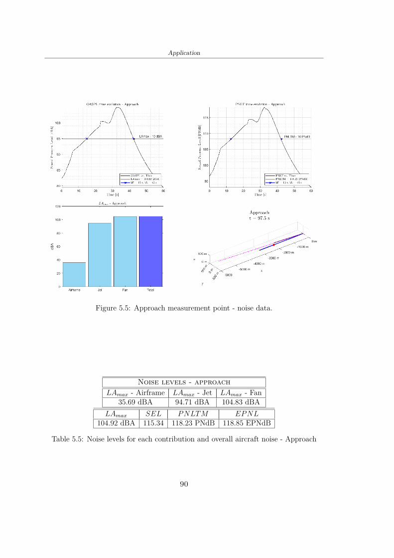
Application
Figure 5.5: Approach measurement point - noise data.
Noise levels - approachLAmax - Airframe LAmax - Jet LAmax - Fan
35.69 dBA 94.71 dBA 104.83 dBALAmax SEL PNLTM EPNL
104.92 dBA 115.34 118.23 PNdB 118.85 EPNdB
Table 5.5: Noise levels for each contribution and overall aircraft noise - Approach
90

Chapter 6
Conclusions and furtherdevelopments
The main motivation for the presented thesis is the development af a methodology ableto introduce noise emission estimation at conceptual design level for a SST aircraft.
Focusing on noise generated during take-off and landing, a first attempt towards thedevelopment of SST aircraft noise prediction routines aiming at predicting several noisemetrics along flyover, departure and approach flight path has been realized. To achievethis objective, a general understanding of the main properties of a comprehensive noiseprediction model has been gained, semi-empirical equations for noise source modellingrelying on aircraft design and operational parameters have been identified and the mostinfluencial parameters amog these have been recognized.
Furhtermore, the overall methodology framework has been described, highlightingthe main components necessary to obtain an estimate of ground-based noise levels froman aircraft moving along a flight path.
At least, a dedicated validation has been performed for LAmax and SEL, using themethodology to get the NPD curves along flyover trajectories and comparing the resultswith the data of the ANP database. Thus, it has been demonstated that the predictionerror falls within the interval [-1.55,1.52] dBA. Moreover, a noise level increment dueto the afterburner has been determined through the evaluation of NPD curves for themaximum wet thrust.
Afterwards, an application of the methodology to the take-off and landing proce-dures defined in the ANP database has been performed. Builing the flight paths fromsegments identified by fixed point data, the trajectories have been simulated and noiselevels at the certification points have been predicted. The results show up that themost dominant noise source during take-off is jet noise, and that the use of the after-burner greatly affects lateral noise level. In addition, approach conditions are the lesscritical for noise generation. However, it has been found that jet and fan noise becomecomparable at this noise and power condition.
91

Conclusions and further developments
Ultimatly, the outcome of this research proved the feasibility of introducing a pre-liminary noise assessment at a conceptual design level for SST aircraft and, as a con-sequence, the possibility to support decision-making process in the early stages of thedesign process in order to mitigate noise generation in the vicinity of airports.
Therefore, with appropriate improvements in noise source and engine modelling,the methodology can be useful to provide guidelines for the design of future low-noiseSST together with operational procedures able to mitigate the LTO noise.
In particular, some examples to improve the noise model, gaining an high-fidelitylevel and extending its capability in the identification of low-noise designs, could includethe modelling of more complex nozzles, such as plug and/or chevron nozzle, or theevaluation of the impact in noise reduction of jet noise suppression measures.
At least, to reach a complete assessment of the acoustic impact of SST aircraft, asa possible future development it could be thought of including within the developedframework additional modules dedicated to the evaluation of the sonic boom, throughappropriate models and definition of the entire profile mission of the aircraft.
92

Appendix A
Main noise sources
Noise sources Noise generating mechanism Relevant parametersLanding gear Broadband noise due to - Length and number of strut
turbolent flow on various - Diameter and number of wheelselement of landing gear - Number of gears and gears doorsand tonal noise due to cavities - Inflow speed
Flaps Broadband noise due to - Flaps deflection angleturbolence around side - Local inflow velocityedges and gaps - Chord length
- Angle of attack- Slat deflection angle- Sweep angle
Slats Broadband noise due to - Local inflow velocityturbolence in gaps - Chord length
- Sweep angle- Geometry between slat- and wing, e.g. gap- height and overlap
Lift and Broadband noise due to - Turbolent intensity at the trailing edgecontrol surfaces turbolence at trailing edge - Sweep angle
- Geometry/shape of the trailing edgeSpoilers Detached flow - Spoiler geometryand speed brakes turbolence at trailing edge - Flight velocityKrueger (leading Not understood - Geometryedge device) - Inflow velocity
- Sweep angle
Table A.1: Overview of airframe noise sources [33]
93

Main noise sources
Noise sources Noise generating mechanism Relevant parametersFan - Thickness and loading noise - Inlet geometry
- Interaction rotor-stator - Number of blades- Stator vane - Number of vanes- Struts - Fan pressure ratio- Fan-intake interaction e.g. - Relative tip Mach numberengine inlet or pylons - Inlet flow distortion,- Tonal noise due to shock e.g. due to an anglecells on blades (harmonic) of attack or due to- Shock cell interaction with a pylon in front of thenacelle (not harmonic sequence) engine
Jet - Turbolent mixing - Velocity differences- Shock noise (only between the streams,in cruise condition) i.e. free, core and
bypass stream- Temperature- Nozzle diameter- Nozzle type
Combustion -Mainly broadband noise - Temperature- Direct contribution due to - Pressure ratiothe expansion of the gas - Sweep anglemixture in the combustion chamber - Combustion type- Indirect noise contribution (lean, rich)due to the convectionof non-uniformitiesthrough pressure gradientsin the turbine
Turbine Tonal and broadband noise - Number of blades(due to same mechanism as - Number of vanesfan noise generation) - Mach number
- Shaft speed- Axial stage spacing- Number of stages- Exit area- Shaft power
Compressor Tonal and broadband - Same as fannoise similar to fan
Table A.2: Overview of engine noise sources [33]
94

Appendix B
Airframe noise directivity
Figure B.1: Clean delta wing directivity
Figure B.2: Vertical tail directivity.
95

Airframe noise directivity
Figure B.3: Landing gear directivity.
96
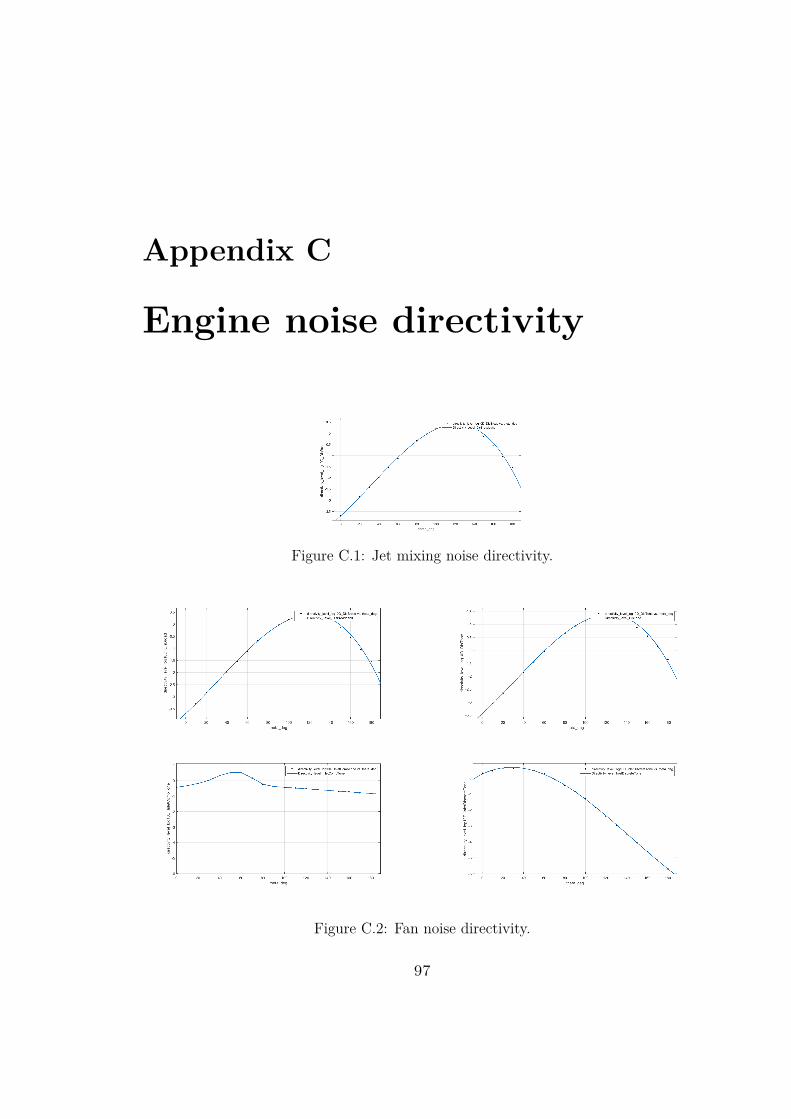
Appendix C
Engine noise directivity
Figure C.1: Jet mixing noise directivity.
Figure C.2: Fan noise directivity.
97

98

Bibliography
[1] IATA: Outlook for the global airline industry, Report, 2019.[2] Boeing: Commericial Market Outlook, Report, 2020-2039.[3] EASA, EEA, Eurocontrol: European Aviation Environmental Report, 2019.[4] ICAO: Environmental Report, 2019.[5] https://hub.united.com[6] Congressional Research Service: Supersonic Passenger Flights, November 2018.[7] M.J.T. Smith: Aircraft Noise, Cambridge Aerospace Series, Cambridge University
Press, ISBN 0-521-61699-9, 2004[8] Schultz TJ: Synthesis of social surveys on noise annoyance J Acoust Soc Am. 1978
Aug;64(2):377-405. doi: 10.1121/1.382013. PMID: 361792.[9] Deborah A. Black, John A. Black, Tharit Issarayangyun, Stephen E. Samuels:
Aircraft noise exposure and resident’s stress and hypertension: A public health per-spective for airport environmental management
[10] Franssen EA, van Wiechen CM, Nagelkerke NJ, Lebret E.: Aircraft noise arounda large international airport and its impact on general health and medicationuse, Occupational and Environmental Medicine. 2004 May;61(5):405-413. doi:10.1136/oem.2002.005488.
[11] J.I. Nijsse: Design and Noise Acceptability of Future Supersonic Transport Aircraft,MSc. Thesis, TU Delft, December 18, 2020.
[12] ICAO: ANNEX 16 to the Convention on International Civil Aviation, Environ-mental Protection. ,Tech. rep., Vol. I (8th edition), ICAO, July 2017.
[13] https://www.icao.int[14] https://rumble-project.eu[15] D. G. Crighton 1991: Aeroacoustics of Flight Vehicles: Theory and Practice: Noise
Sources, NASA Reference Publication 1258, RDC Technical Report 90-3052 (H. H.Hubbard, editor).
[16] ICAO: Guidance on the balanced approach to aircraft noise management, October,2010.
[17] Nicolas E. Antoine, Ilan M. Kroo: Aircraft Optimization for Minimal Environ-mental Impact, Journal Article, Journal of Aircraft July 41 (4): 790, 2004.
[18] Nicolas E. Antoine, Ilan M. Kroo: Framework for Aircraft Conceptual Design andEnvironmental Performance Studies, Journal Article, AIAA Journal October 43(10): 2100, 2005.
99

Bibliography
[19] Andrew March, Ian Waitz and Karen Willcox: A Methodology for Integrated Con-ceptual Design of Aircraft Configuration and Operation to Reduce EnvironmentalImpact, Book Chapter, 9th AIAA Aviation Technology, Integration, and OperationsConference (ATIO) 21-23 September 2009, Hilton Head, South Carolina © 2009 byMassachusetts Institute of Technology.
[20] Filippone, Antonio: Aircraft noise prediction, Progress in Aerospace Sciences, Vol-ume 68, Pages 27-63, ISSN 0376-0421, 2014.
[21] Farassat, F. and Casper, J. H.: Towards an Airframe Noise Prediction Method-ology: Survey of Current Approaches., in 44th AIAA Aerospace Sciences Meetingand Exhibit, 2006. doi:10.2514/6.2006210.
[22] Dobrzynski, Werner: Almost 40 Years of Airframe Noise Research: What Did WeAchieve?, Journal of Aircraft, vol. 47, n.2, pages 353-367, doi:10.2514/1.44457.
[23] Raney, John P., S. L. Padula, and W. E. Zorumski: NASA progress in aircraftnoise prediction, Vol. 81915. National Aeronautics and Space Administration, Sci-entific and Technical Information Branch, 1981.
[24] Leonard Lopes and Casey Burley: Design of the Next Generation Aircraft NoisePrediction Program: ANOPP2, 17th AIAA/CEAS Aeroacoustics Conference (32ndAIAA Aeroacoustics Conference), https://arc.aiaa.org/doi/abs/.
[25] Bertsch, Lothar and Isermann, Ullrich: Tool Development for Low-Noise AircraftDesign, Journal of Aircraft, vol. 47, n. 2, pages 694-699, doi: 10.2514/1.43188,2010.
[26] Filippone, Antonio and Bertsch, Lothar and Pott-Pollenske, Michael: Validationstrategies for comprehensive aircraft noise prediction methods, 2012.
[27] J.R. Olmstead, G.G. Fleming, J.M. Gulding, C.J. Roof, P.J. Gerbi, and A.S.Rapoza: Integrated Noise Model (INM) Version 6.0 Technical Manual, U.S. Depart-ment of Transportation Federal Aviation Administration, Report No. FAA-AEE-02-01, January 2002,Washington, D.C., USA
[28] ECAC.CEAC Doc 29: Report on Standard Method of Computing Noise Contoursaround Civil Airports, Volume 3, Part 1 - Reference Cases and Verification Frame-work, 7 December, 2016.
[29] Bertsch, Lothar and Isermann, Ullrich: Noise prediction toolbox used by the DLRaircraft noise working group, INTER-NOISE and NOISE-CON Congress and Con-ference Proceedings, 2013.
[30] Bertsch L., Noise Prediction within Conceptual Aircraft Design, PhD thesis, Insti-tute of Aerodynamics and Flow Technology, DLR, Braunschweig, 2013.
[31] Wilson, M.: An introduction to high speed aircraft noise prediction., 1992.[32] R.E. Gillian: Aircraft Noise Prediction Program User’s Manual, NASA Langley
Research Center, 1982.[33] Bertsch, L., Simons, D., Snellen, M.: Aircraft Noise: The major sources, modelling
capabilities, and reduction possibilities, (IB 224-2015 A 110 ed.) DLR, 2015.[34] Fink, Martin R.,Noise Component Method for Airframe Noise, Journal of Aircraft,
vol. 16, n. 10, pages 656-665,1979, doi:10.2514/3.58586.[35] M.R. Fink: Airframe Noise Prediction Method, FAA Research Report, FAA-RD-
77-29, March 1977.
100

Bibliography
[36] Stone, James R., and Frances J. Montegani: An improved prediction method forthe noise generated in flight by circular jets, 1980.
[37] Stone, James R.: Interim prediction method for jet noise, 1974.[38] Barbosa, Joao and Dezan, Daniel: Single-Stream Jet Noise Prediction Using Em-
pirical Methodology for a Newly Designed Turbojet Engine, Proceedings of theASME Turbo Expo, doi: 10.1115/GT2013-95199, 2013.
[39] Almeida, Odenir: Semi-Empirical Methods for Coaxial Jet Noise Prediction, 2008.[40] Heidmann, M.: Interim prediction method for fan and compressor source noise,
1975.[41] Gregorio Stiuso: Tecnica di simulazione numerica delle prestazioni
stazionarie e transitorie di turbomotori., Rel. Michele Ferlauto. Politec-nico di Torino, Corso di laurea magistrale in Ingegneria Aerospaziale,2019.URI:http://webthesis.biblio.polito.it/id/eprint/11258.
[42] Stitt, L. E.:Exhaust Nozzles for Propulsion Systems with Emphasis on SupersonicCruise Aircraft., 1990.
[43] Vasov, Ljubiša and Stojiljkovic, Branimir and Cokorilo, Olja and Mirosavljevic,Petar and Gvozdenovic, Slobodan: Aircraft noise metrics, Journal Safety Engineer-ing, vol. 4, December, 2014, doi: 10.7562/SE2014.4.02.04.
[44] ERCD Report 0904: Metrics for Aircraft Noise,January 20, 2009.[45] Bennett, R. L., Pearsons, K. S: Handbook of aircraft noise metrics, Contractor
Report (CR), March 1, 1981[46] A-21 Aircraft Noise Measurement Aviation Emission Modeling: Standard Values
of Atmospheric Absorption as a Function of Temperature and Humidity, ARP 866B,December, 2021, doi: https://doi.org/10.4271/ARP866B.
[47] Jane’s All the world’s aircraft, 1965-66.[48] Jane’s All the world’s aircraft, 1974-75.[49] Underwood, Matthew C: Concept of operations for integrating commercial super-
sonic transport aircraft into the national airspace system, 2017.[50] www.aircraftnoisemodel.org[51] Directive 2002/49/EC of the European Parliament and of the Council, 25 June
2002.[52] Cooper, Steven:Problems with the INM: Part 3 - Derivation of NPD Curves,
Cooper2006ProblemsWT, 2006.[53] Cooper, Steven and Maung, John:Problems with the INM: Part 2 – Atmospheric
Attenuation, Cooper2006ProblemsWT, 2006.[54] ECAC.CEAC Doc 29, 4th ed.:Report on Standard Method of Computing Noise
Contours Around Civil Airports, proceedings of the European Civil AviationConference, European Civil Aviation Conference (ECAC) Document 29, Paris,https://www.ecac-ceac.org/ecac-docs [retrieved 7 Dec. 2016].
101