ludwigs-maximilians-universitat m¨ ¨unchen university ... · — departement for physics —...
TRANSCRIPT

Ludwigs-Maximilians-Universitat Munchen— Departement for Physics —
University Observatory
Computational Methods in Astrophysics
Ordinary Differential Equations
—
Cosmological Models
second, completely revised edition (2007)
Joachim Puls/Fabian Heitsch
winter semester 2007/2008
Foreword
This is an instruction set for a lab course on Ordinary Differential Equations. As such, it isneither complete nor perfect (and we’re not talking about typos here).
From your point of view, the former can be a cause of nuisance and – in most cases – a sourcefor additional work. This is intended. The script cannot replace reading the original literature.Wherever appropriate, we have tried to point to the relevant papers/books.
We would greatly appreciate any feedback on inconsistencies, mistakes, obvious blunders andoutright nonsense in the script. Also, we’d be very thankful for suggestions how to improve thescript beyond the afore-mentioned.
Despite these ominous beginnings, we hope you’ll enjoy the following. After all, numerics area never-ending source of surprises!
ii
Contents
1 Introduction 1-11.1 Why Ordinary Differential Equations? . . . . . . . . . . . . . . . . . . . . . . . . 1-1
2 Numerics 2-12.1 Facts about ODEs . . . . . . . . . . . . . . . . . . . . . . . . . . . . . . . . . . . 2-1
2.1.1 Existence and uniqueness . . . . . . . . . . . . . . . . . . . . . . . . . . . 2-12.2 Consistency, convergence and discretization errors . . . . . . . . . . . . . . . . . 2-22.3 Single-step methods . . . . . . . . . . . . . . . . . . . . . . . . . . . . . . . . . . 2-5
2.3.1 Euler method . . . . . . . . . . . . . . . . . . . . . . . . . . . . . . . . . 2-62.3.2 Generalized Runge-Kutta methods . . . . . . . . . . . . . . . . . . . . . . 2-9
2.4 Step-size control . . . . . . . . . . . . . . . . . . . . . . . . . . . . . . . . . . . . 2-142.4.1 Error estimate from step doubling . . . . . . . . . . . . . . . . . . . . . . 2-152.4.2 Embedded methods . . . . . . . . . . . . . . . . . . . . . . . . . . . . . . 2-162.4.3 Defining the tolerance level . . . . . . . . . . . . . . . . . . . . . . . . . . 2-17
2.5 Absolute Stability. Stiff sets of differential equations . . . . . . . . . . . . . . . . 2-182.6 Semi-implicit methods . . . . . . . . . . . . . . . . . . . . . . . . . . . . . . . . . 2-22
3 Physics – Cosmological Models 3-13.1 Cosmological redshift and Hubble’s law . . . . . . . . . . . . . . . . . . . . . . . 3-13.2 Newtonian expansion . . . . . . . . . . . . . . . . . . . . . . . . . . . . . . . . . . 3-33.3 Robertson-Walker metric . . . . . . . . . . . . . . . . . . . . . . . . . . . . . 3-53.4 Friedmann cosmologies . . . . . . . . . . . . . . . . . . . . . . . . . . . . . . . . 3-63.5 Cosmological constant . . . . . . . . . . . . . . . . . . . . . . . . . . . . . . . . . 3-93.6 Friedmann-Lemaıtre cosmologies . . . . . . . . . . . . . . . . . . . . . . . . . 3-103.7 Energy conservation and equation of state . . . . . . . . . . . . . . . . . . . . . . 3-123.8 Evolution of the scale factor . . . . . . . . . . . . . . . . . . . . . . . . . . . . . . 3-13
4 Experiment 4-14.1 Numerical solution of ODEs: Test problems and integrators . . . . . . . . . . . . 4-1
4.1.1 The programs . . . . . . . . . . . . . . . . . . . . . . . . . . . . . . . . . . 4-14.1.2 Problem 1 – A first test . . . . . . . . . . . . . . . . . . . . . . . . . . . . 4-14.1.3 Stiff Equations . . . . . . . . . . . . . . . . . . . . . . . . . . . . . . . . . 4-24.1.4 ADVANCED: Problem 4 – Accuracy and rounding errors . . . . . . . . . 4-3
4.2 Friedmann-Lemaıtre cosmologies: numerical solutions . . . . . . . . . . . . . . 4-54.2.1 Implementation and first tests . . . . . . . . . . . . . . . . . . . . . . . . 4-54.2.2 Solutions for various parameter combinations . . . . . . . . . . . . . . . . 4-5
iii

CONTENTS
iv

Chapter 1
Introduction
1.1 Why Ordinary Differential Equations?
Differential equations (DEs) are omnipresent once it comes to determining the dynamical evolu-tion, the structure, or the stability of physical systems. In many cases, the resulting set of DEscontains several independent variables (e.g., spatial coordinates and time in hydrodynamics), inwhich case the DEs are called partial differential equations (PDEs). These will be of no concernhere.
However, often, it is possible to simplify the set of DEs by physical reasoning such that thenumber of independent variables is reduced to 1, in which case we speak of ordinary differentialequations (ODEs): The classical stellar structure models neglect time evolution and non-sphericaleffects, resulting in coupled differential equations only depending on the radius or the masscoordinate. Likewise, chemical networks are often formulated locally, i.e. the (coupled) rateequations depend only on time.
The solving ”strategy” (at least for initial value problems) in most cases boils down to: (0)Choose the appropriate solution method (“solver”), in dependence of the properties of the ODEs(and their solution functions). (1) Determine the initial conditions. (2) Find the appropriate stepsize (3) advance the solution by that step size. (4) Repeat [2] and [3]. Of course, the problemsarise in the steps (2) and (3). What is the correct step size, and how should we integrate theequations? This entails problems like: How large are the errors we make? And, how much canwe trust the solutions? The rest of this script centers around these questions, and attempts tothrow some light on possible answers with the help of some examples.
There is a whole wealth of possible applications of ODEs in physics/astronomy. However,instead of (re-)introducing the Kepler-problem or the differential equations describing stellarstructure, we will (finally) use the Friedmann-Lemaıtre equation(s) describing the temporalevolution of our cosmos to shed some light on how to integrate ODEs numerically, and to obtainan impression of what can go wrong if one has no theoretical background.
For this purpose (but also in order to tackle different equations underlying different problems– e.g., so-called stiff problems), we need the integrators and techniques which are introduced inChap. 2, after we have briefly recapitulated some basic facts (including the (in?)famous theoremof Picard-Lindelof which shows under which conditions ODEs can be solved uniquely).
Chap. 3 gives a short introduction into cosmological models, concentrating on the derivationof the Friedmann-Lemaıtre-equations and related problems. As a major outcome, we willformulate the final equation for the temporal evolution of the “cosmic scale factor”, which hasto be solved in dependence of total matter-/radiation-density and cosmological constant, which
1-1

CHAPTER 1. INTRODUCTION
is interpreted as “dark energy” nowadays.After all this, we finally get to the experiments themselves in Chap. 4. On the first day of our
lab work, we will investigate different techniques to solve ODEs, at hand of three different exam-ples. On the second day then, we will apply our accumulated knowledge to solve the Friedmann-Lemaıtre-equation under various conditions. A highlight will be the re-construction of the fa-mous ΩM vs. ΩΛ diagram (e.g., Perlmutter et al. 1999), which allows to understand the variouspossibilities for the future fate of our and other cosmoses, in dependence of total matter-densityand cosmological constant.
Due to the above layout of the “experimental” work, we suggest the following schedule for afruitful preparation:
Before day 1: Study the numerical methods (Chap. 2), and have a look into the problems to besolved on the first day (Sect. 4.1).
Before day 2: Study the introduction into cosmological models (Chap. 3), and refer to the liter-ature in case of problems. Inform yourself on the experiments/problems planned for the secondday (Sect. 4.2). In order to be able to solve some of these problems, we suggest to work onExercises 5 and 6 also before day 2.
1-2
Chapter 2
Numerics
2.1 Some general facts about ODEs
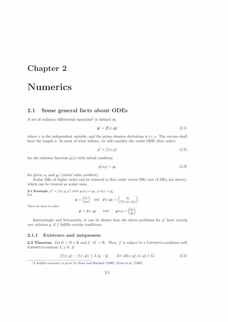
A set of ordinary differential equations1 is defined as,
y′ = f(x,y) (2.1)
where x is the independent variable, and the prime denotes derivation w.r.t x. The vectors shallhave the length n. In most of what follows, we will consider the scalar ODE (first order)
y′ = f(x, y) (2.2)
for the solution function y(x) with initial condition
y(x0) = y0 (2.3)
for given x0 and y0 (initial value problem).Scalar DEs of higher order can be reduced to first order vector DEs (set of DEs, see above),
which can be treated as scalar ones.
2.1 Example. y′′ = f(x, y, y′) with y(x0) = y0, y′(x0) = y′
0.Let
y :=
„
y1
y2
«
and f(x, y) :=
„
y2
f(x, y1, y2)
«
.
Then we have to solve
y′ = f(x, y) with y(x0) =
„
y0
y′
0
«
Interestingly and fortunately, it can be shown that the above problems for y′ have exactlyone solution y, if f fulfills certain conditions.
2.1.1 Existence and uniqueness
2.2 Theorem. Let G ⊂ R×R and f : G → R. Then, f is subject to a Lipshitz-condition withLipshitz-constant L ≥ 0, if
|f(x, y) − f(x, y)| ≤ L |y − y| for all(x, y), (x, y) ∈ G. (2.4)
1A helpful summary is given by Stoer and Burlisch (1990); Press et al. (1992)
2-1
CHAPTER 2. NUMERICS
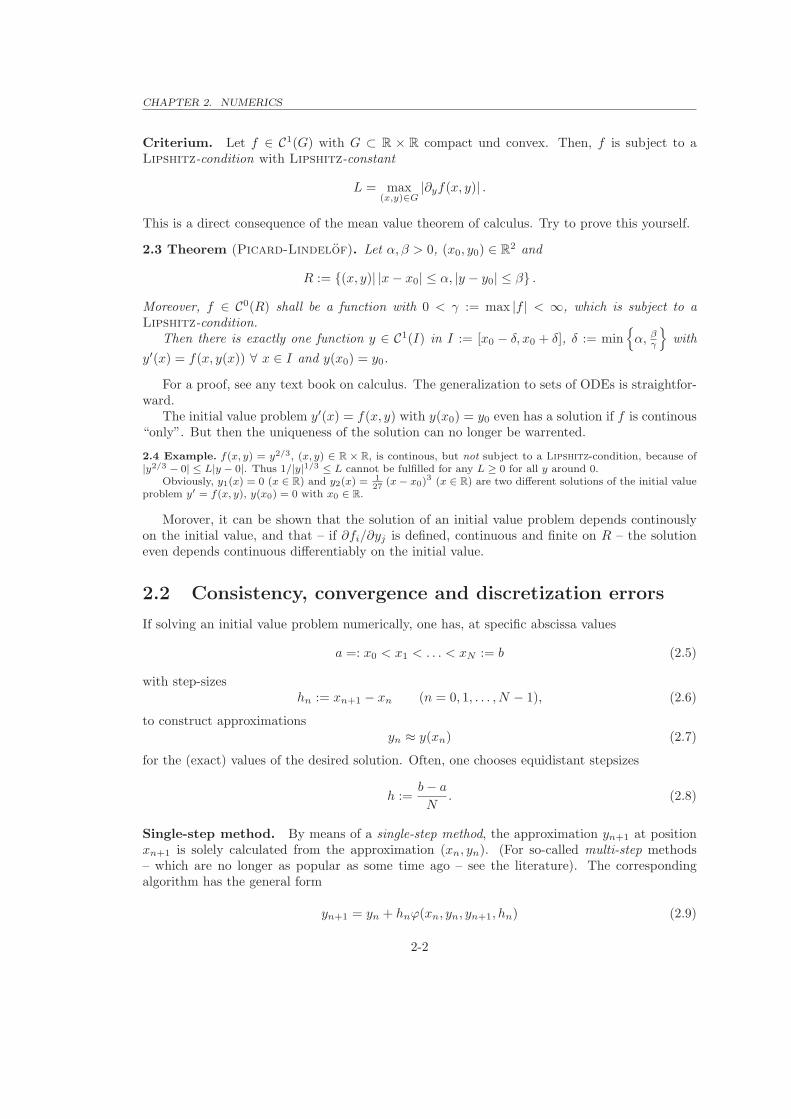
Criterium. Let f ∈ C1(G) with G ⊂ R × R compact und convex. Then, f is subject to aLipshitz-condition with Lipshitz-constant
L = max(x,y)∈G
|∂yf(x, y)| .
This is a direct consequence of the mean value theorem of calculus. Try to prove this yourself.
2.3 Theorem (Picard-Lindelof). Let α, β > 0, (x0, y0) ∈ R2 and
R := (x, y)| |x − x0| ≤ α, |y − y0| ≤ β .
Moreover, f ∈ C0(R) shall be a function with 0 < γ := max |f | < ∞, which is subject to aLipshitz-condition.
Then there is exactly one function y ∈ C1(I) in I := [x0 − δ, x0 + δ], δ := min
α, βγ
with
y′(x) = f(x, y(x)) ∀ x ∈ I and y(x0) = y0.
For a proof, see any text book on calculus. The generalization to sets of ODEs is straightfor-ward.
The initial value problem y′(x) = f(x, y) with y(x0) = y0 even has a solution if f is continous“only”. But then the uniqueness of the solution can no longer be warrented.
2.4 Example. f(x, y) = y2/3, (x, y) ∈ R × R, is continous, but not subject to a Lipshitz-condition, because of|y2/3 − 0| ≤ L|y − 0|. Thus 1/|y|1/3 ≤ L cannot be fulfilled for any L ≥ 0 for all y around 0.
Obviously, y1(x) = 0 (x ∈ R) and y2(x) = 127
(x − x0)3 (x ∈ R) are two different solutions of the initial valueproblem y′ = f(x, y), y(x0) = 0 with x0 ∈ R.
Morover, it can be shown that the solution of an initial value problem depends continouslyon the initial value, and that – if ∂fi/∂yj is defined, continuous and finite on R – the solutioneven depends continuous differentiably on the initial value.
2.2 Consistency, convergence and discretization errors
If solving an initial value problem numerically, one has, at specific abscissa values
a =: x0 < x1 < . . . < xN := b (2.5)
with step-sizeshn := xn+1 − xn (n = 0, 1, . . . , N − 1), (2.6)
to construct approximationsyn ≈ y(xn) (2.7)
for the (exact) values of the desired solution. Often, one chooses equidistant stepsizes
h :=b − a
N. (2.8)
Single-step method. By means of a single-step method, the approximation yn+1 at positionxn+1 is solely calculated from the approximation (xn, yn). (For so-called multi-step methods– which are no longer as popular as some time ago – see the literature). The correspondingalgorithm has the general form
yn+1 = yn + hnϕ(xn, yn, yn+1, hn) (2.9)
2-2

CHAPTER 2. NUMERICS
where ϕ is a specific, algorithm dependent function. If ϕ does not depend on yn+1, we talk aboutan explicit single-step methods, otherwise about an implicit single-step method.
In the latter case, an implicit equation for yn+1 has to be solved (numerically). This is thedisadvantage of the implicit method. Its advantage is given by its stability (see Sect. 2.5).
Let us now consider the error (w.r.t. the exact solution) which has accumulated after acertain number of steps. At first, we will neglect rounding-errors. In the following, we willrestrict ourselves to equidistant step-sizes.
Global discretization error. The global discretization error at position xn measures thedifference
gn := y(xn) − yn (n = 0, 1, . . . , N). (2.10)
The single-step method is called convergent, if
maxn=0,1,...,N
|gn| → 0 for h → 0+. (2.11)
Such a method has a convergence order p > 0, if the global discretization error can be writtenin the form
maxn=0,1,...,N
|gn| ≤ chp = O(hp), (2.12)
with constants c ≥ 0 und p > 0 independent of h. To obtain useful estimates for the globaldiscretization error, we have also to define a
Local discretization error, which is defined (at position xn+1) by
ln+1 := y(xn+1) − y(xn) − hϕ(xn, y(xn), y(xn+1), h). (2.13)
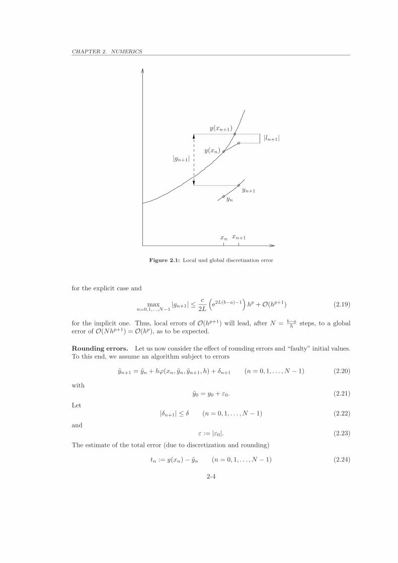
This local error describes the deviation of the exact solution from the algorithm function. Foran explicit method, ln+1 is the difference between exact value y(xn+1) und approximation yn+1,if we would start at xn with the exact value y(xn) (error of one step; see Fig. 2.1).
A single-step method is called consistent, if
1
hln+1 → 0 fur h → 0+ (n = 0, 1, . . . , N − 1). (2.14)
Because ofln+1
h=
y(xn+1) − y(xn)
h︸ ︷︷ ︸
secant slope of exact solution
−ϕ(xn, y(xn), y(xn+1), h)︸ ︷︷ ︸
approximation of this slope
, (2.15)
we have the equivalence of
1
h|ln+1|
h→0+
−−−−→ 0 ⇔ ϕ(xn, y(xn), y(xn+1), h)h→0+
−−−−→ f(xn, y(xn)). (2.16)
The method has a consistency order (brief: order) of p, if the local discretization error fulfillsthe inequality
|ln+1| ≤ chp+1 = O(hp+1) (2.17)
with constants c ≥ 0 and p > 0, independent of h.We are now able to relate the global with the local discretization error. For a method of
consistency order p and an ODE with function y subject to a Lipshitz constant L, we finallyobtain after some effort
maxn=0,1,...,N−1
|gn+1| ≤c
L
(
eL(b−a) − 1)
hp (2.18)
2-3
CHAPTER 2. NUMERICS
|gn+1|y(xn)
y(xn+1)
xn xn+1
yn
yn+1
|ln+1|
Figure 2.1: Local und global discretization error
for the explicit case and
maxn=0,1,...,N−1
|gn+1| ≤c
2L
(
e2L(b−a)−1)
hp + O(hp+1) (2.19)
for the implicit one. Thus, local errors of O(hp+1) will lead, after N = b−ah steps, to a global
error of O(Nhp+1) = O(hp), as to be expected.
Rounding errors. Let us now consider the effect of rounding errors and “faulty” initial values.To this end, we assume an algorithm subject to errors
yn+1 = yn + hϕ(xn, yn, yn+1, h) + δn+1 (n = 0, 1, . . . , N − 1) (2.20)
withy0 = y0 + ε0. (2.21)
Let|δn+1| ≤ δ (n = 0, 1, . . . , N − 1) (2.22)
andε := |ε0|. (2.23)
The estimate of the total error (due to discretization and rounding)
tn := y(xn) − yn (n = 0, 1, . . . , N − 1) (2.24)
2-4

CHAPTER 2. NUMERICS
00
Total error
discretization error ∼ hp
rounding error ∼ 1/h
step-sizehopt.
Figure 2.2: Total error due to discretization and rounding
can be obtained quite similar to the case without rounding errors, and results in
maxn=0,1,...,N−1
|tn+1| ≤ eL(b−a)ε +1
L
(
eL(b−a) − 1)(
chp +δ
h
)
(2.25)
for the explicit case and
maxn=0,1,...,N−1
|tn+1| ≤ eL(b−a)ε +1
2L
(
e2L(b−a)/(1−Lh) − 1)(
chp +δ
h
)
(2.26)
for the implicit one. Particularly, we obtain
maxn=0,1,...,N−1
|tn+1| ≤1
L
(
eL(b−a) − 1)(
chp +δ
h
)
(2.27)
for the explicit, single-step method with exact initial values.
Exercise 1: For the latter case, calculate the optimum step-size.
2.3 Single-step methods
Let y(x) be the solution of the DE y′ = f(x, y). If the graph of this solution passes through apoint (x, y), the slope of this graph at this point is f(x, y): The value f(x, y) fixes the slope of the
2-5
CHAPTER 2. NUMERICS
−2 −1.5 −1 −0.5 0 0.5 1
1
1.5 2
2
0.4
0.6
0.8
1.2
1.4
1.6
1.8
Figure 2.3: Directional field for example 2.5
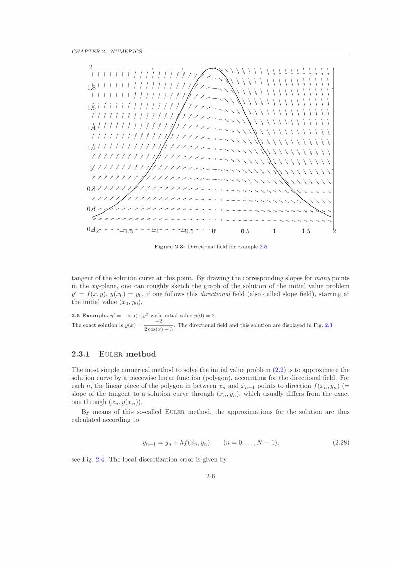
tangent of the solution curve at this point. By drawing the corresponding slopes for many pointsin the xy-plane, one can roughly sketch the graph of the solution of the initial value problemy′ = f(x, y), y(x0) = y0, if one follows this directional field (also called slope field), starting atthe initial value (x0, y0).
2.5 Example. y′ = − sin(x)y2 with initial value y(0) = 2.
The exact solution is y(x) =−2
2 cos(x) − 3. The directional field and this solution are displayed in Fig. 2.3.
2.3.1 Euler method
The most simple numerical method to solve the initial value problem (2.2) is to approximate thesolution curve by a piecewise linear function (polygon), accounting for the directional field. Foreach n, the linear piece of the polygon in between xn and xn+1 points to direction f(xn, yn) (=slope of the tangent to a solution curve through (xn, yn), which usually differs from the exactone through (xn, y(xn)).
By means of this so-called Euler method, the approximations for the solution are thuscalculated according to
yn+1 = yn + hf(xn, yn) (n = 0, . . . , N − 1), (2.28)
see Fig. 2.4. The local discretization error is given by
2-6

CHAPTER 2. NUMERICS
x
y
x0 x1 x2 x3
y0 y1 y2 y3
y(x)
Figure 2.4: Euler method
ln+1 = y(xn+1)︸ ︷︷ ︸
(∗)
−y(xn) − hf(xn, y(xn)
)
=1
2
(
∂xf(xn, y(xn)
)+ f
(xn, y(xn)
)∂yf
(xn, y(xn)
))
h2 + O(h3), (2.29)
using the Taylor expansion
(∗) = y(xn) + y′(xn)h +1
2y′′(xn)h2 + O(h3)
= y(xn) + f(xn, y(xn)
)h +
1
2
(
∂xf(xn, y(xn)
)+ f
(xn, y(xn)
)∂yf
(xn, y(xn)
))
h2 + O(h3).
Thus, the consistency order of the Euler method is p = 1.
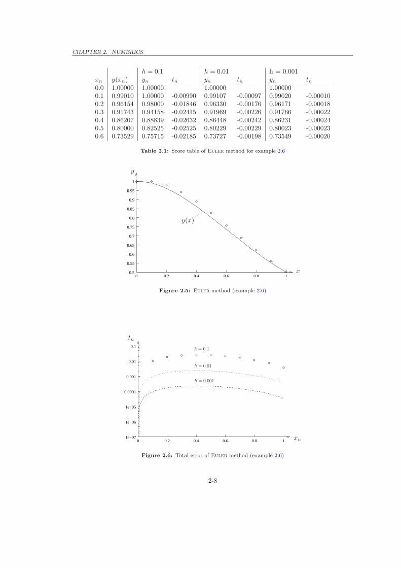
2.6 Example. y′ = −2xy2, y(0) = 1. Table 2.1 displays the results using the Euler method, for differentstep-sizes (see also Fig. 2.5). Fig. 2.6 shows the corresponding total error, which decreases (roughly) proportional
to step-size. The exact solution is y(x) =1
1 + x2.
2-7
CHAPTER 2. NUMERICS
h = 0.1 h = 0.01 h = 0.001xn y(xn) yn tn yn tn yn tn0.0 1.00000 1.00000 1.00000 1.000000.1 0.99010 1.00000 -0.00990 0.99107 -0.00097 0.99020 -0.000100.2 0.96154 0.98000 -0.01846 0.96330 -0.00176 0.96171 -0.000180.3 0.91743 0.94158 -0.02415 0.91969 -0.00226 0.91766 -0.000220.4 0.86207 0.88839 -0.02632 0.86448 -0.00242 0.86231 -0.000240.5 0.80000 0.82525 -0.02525 0.80229 -0.00229 0.80023 -0.000230.6 0.73529 0.75715 -0.02185 0.73727 -0.00198 0.73549 -0.00020
Table 2.1: Score table of Euler method for example 2.6
0.5
0.55
0.6
0.65
0.7
0.75
0.8
0.85
0.9
0.95
1
0 0.2 0.4 0.6 0.8 1x
y
y(x)
Figure 2.5: Euler method (example 2.6)
1e−07
1e−06
1e−05
0.0001
0.001
0.01
0.1
0 0.2 0.4 0.6 0.8 1
tn
xn
h = 0.1
h = 0.01
h = 0.001
Figure 2.6: Total error of Euler method (example 2.6)
2-8
CHAPTER 2. NUMERICS
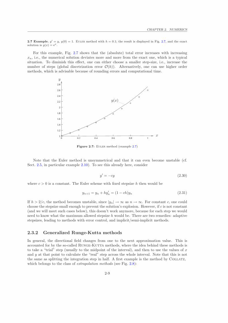
2.7 Example. y′ = y, y(0) = 1. Euler method with h = 0.1; the result is displayed in Fig. 2.7, and the exactsolution is y(x) = ex.
For this example, Fig. 2.7 shows that the (absolute) total error increases with increasingxn, i.e., the numerical solution deviates more and more from the exact one, which is a typicalsituation. To diminish this effect, one can either choose a smaller step-size, i.e., increase thenumber of steps (global discetrization error O(h)). Alternatively, one can use higher ordermethods, which is advisable because of rounding errors and computational time.
1
1.2
1.4
1.6
1.8
2
2.2
2.4
2.6
2.8
0 0.2 0.4 0.6 0.8 1x
y
y(x)
Figure 2.7: Euler method (example 2.7)
Note that the Euler method is unsymmetrical and that it can even become unstable (cf.Sect. 2.5, in particular example 2.10). To see this already here, consider
y′ = −cy (2.30)
where c > 0 is a constant. The Euler scheme with fixed stepsize h then would be
yn+1 = yn + hy′n = (1 − ch)yn (2.31)
If h > 2/c, the method becomes unstable, since |yn| → ∞ as n → ∞. For constant c, one couldchoose the stepsize small enough to prevent the solution’s explosion. However, if c is not constant(and we will meet such cases below), this doesn’t work anymore, because for each step we wouldneed to know what the maximum allowed stepsize h would be. There are two remedies: adaptivestepsizes, leading to methods with error control, and implicit/semi-implicit methods.
2.3.2 Generalized Runge-Kutta methods
In general, the directional field changes from one to the next approximation value. This isaccounted for by the so-called Runge-Kutta methods, where the idea behind these methods isto take a “trial” step (usually to the midpoint of the interval), and then to use the values of xand y at that point to calculate the “real” step across the whole interval. Note that this is notthe same as splitting the integration step in half. A first example is the method by Collatz,which belongs to the class of extrapolation methods (see Fig. 2.8):
2-9

CHAPTER 2. NUMERICS
k1 := f(xn, yn) ,
k2 := f
(
xn +h
2, yn +
h
2k1
)
;
yn+1 = yn + h · k2 (2.32)
The local discretization error can be shown to have the structure
xn xn+1/2 xn+1
yn
yn+1/2
yn+1k1
k2
Figure 2.8: Collatz method
ln+1 = F (xn, y(xn))h3 + O(h4), (2.33)
since the symmetrization cancels out the first and 2nd order terms in h. Thus, this method hasa consistency order of p = 2.
2.8 Example (continuation of example 2.6). Score table of Collatz method:
h = 0.1 h = 0.05xn yn tn yn tn0.0 1.00000 1.000000.1 0.99000 0.00010 0.99007 0.000020.2 0.96118 0.00036 0.96145 0.000090.3 0.91674 0.00069 0.91727 0.000160.4 0.86110 0.00096 0.86184 0.000230.5 0.79889 0.00111 0.79974 0.000260.6 0.73418 0.00111 0.73503 0.000260.7 0.67014 0.00100 0.67091 0.000230.8 0.60895 0.00080 0.60957 0.000180.9 0.55191 0.00058 0.55236 0.000131.0 0.49964 0.00036 0.49992 0.00008
For same step-size, the total errors are (absolutely) smaller than for the Euler method. Comparing differentstep-sizes, the consistency order of p = 2 is obvious.
2-10

CHAPTER 2. NUMERICS
In order to develop methods of higher order, some systematic procedure is required. To thisend, we integrate the DE y′(x) = f(x, y(x)) over the interval [xn, xn+1] of length h = xn+1 − xn
w.r.t. the independent variable x:
y(xn+1) = y(xn) +
xn+1∫
xn
f(x, y(x))dx. (2.34)
Note that the initial value problem (2.2) is equivalent to the integral equation
y(x) = y0 +
x∫
x0
f(x′, y(x′))dx′. (2.35)
The integral (2.34) is approximated by quadrature formulas (cf. Numerical Lab Course “Inte-gration”)
xn+1∫
xn
f(x, y(x))dx ≈ h
m∑
r=1
γr f (xn + αrh, y(xn + αrh)) (2.36)
with weights γr ≥ 0 and abscissa values (“knots”) xn + αrh with 0 ≤ αr ≤ 1 (r = 1, 2, . . . ,m),α1 := 0.
The major problem now is that the y(xn+αrh) in (2.36) are unknown and have to be replacedby approximations, using the following ansatz:
f(xn + α1h, y(xn + α1h)) =: k1(xn, y(xn)),
f(xn + α2h, y(xn + α2h)) ≈ f (xn + α2h, y(xn) + hβ21k1(xn, y(xn)))
=: k2(xn, y(xn)),
f(xn + α3h, y(xn + α3h)) ≈ f (xn + α3h, y(xn) + h (β31k1(xn, y(xn)) + β32k2(xn, y(xn))))
=: k3(xn, y(xn))
...
f(xn + αmh, y(xn + αmh)) ≈ f
(
xn + αmh, y(xn) + h
m−1∑
s=1
βmsks(xn, y(xn))
)
=: km(xn, y(xn)) (2.37)
with constants βrs. One requires
r−1∑
s=1
βrs = αr, (r = 2, 3, . . . ,m), (2.38)
so that the approximations (2.37) are exact at least to O(h). This follows from the Taylorexpansion in step-size:
f(xn + αrh, y(xn + αrh)) − f
(
xn + αrh, y(xn) + h
r−1∑
s=1
βrsks(xn, y(xn))
)
=
=
(
αr −
r−1∑
s=1
βrs
)
f(xn, y(xn)) ∂yf(xn, y(xn))h + O(h2). (2.39)
2-11
CHAPTER 2. NUMERICS
α1
α2 β21
α3 β31 β32
...αm βm1 βm2 · · · βm,m−1
γ1 γ2 · · · γm−1 γm
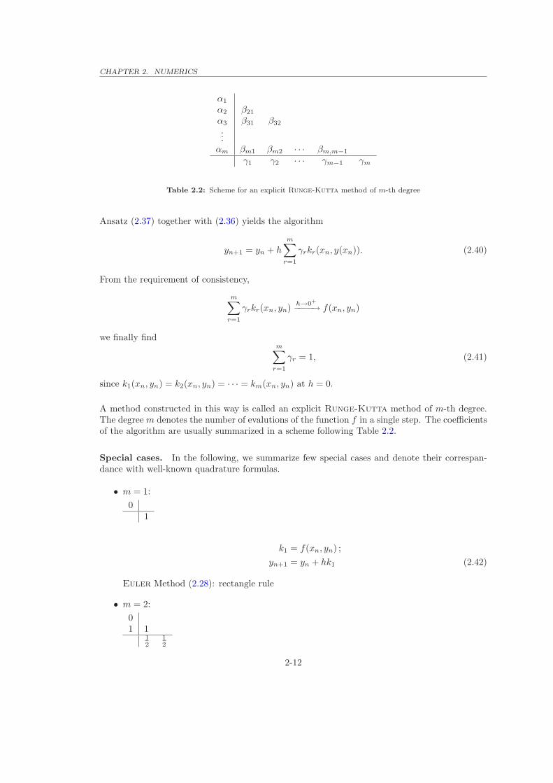
Table 2.2: Scheme for an explicit Runge-Kutta method of m-th degree
Ansatz (2.37) together with (2.36) yields the algorithm
yn+1 = yn + h
m∑
r=1
γrkr(xn, y(xn)). (2.40)
From the requirement of consistency,
m∑
r=1
γrkr(xn, yn)h→0+
−−−−→ f(xn, yn)
we finally findm∑
r=1
γr = 1, (2.41)
since k1(xn, yn) = k2(xn, yn) = · · · = km(xn, yn) at h = 0.
A method constructed in this way is called an explicit Runge-Kutta method of m-th degree.The degree m denotes the number of evalutions of the function f in a single step. The coefficientsof the algorithm are usually summarized in a scheme following Table 2.2.
Special cases. In the following, we summarize few special cases and denote their correspan-dance with well-known quadrature formulas.
• m = 1:
01
k1 = f(xn, yn) ;
yn+1 = yn + hk1 (2.42)
Euler Method (2.28): rectangle rule
• m = 2:
01 1
12
12
2-12
CHAPTER 2. NUMERICS
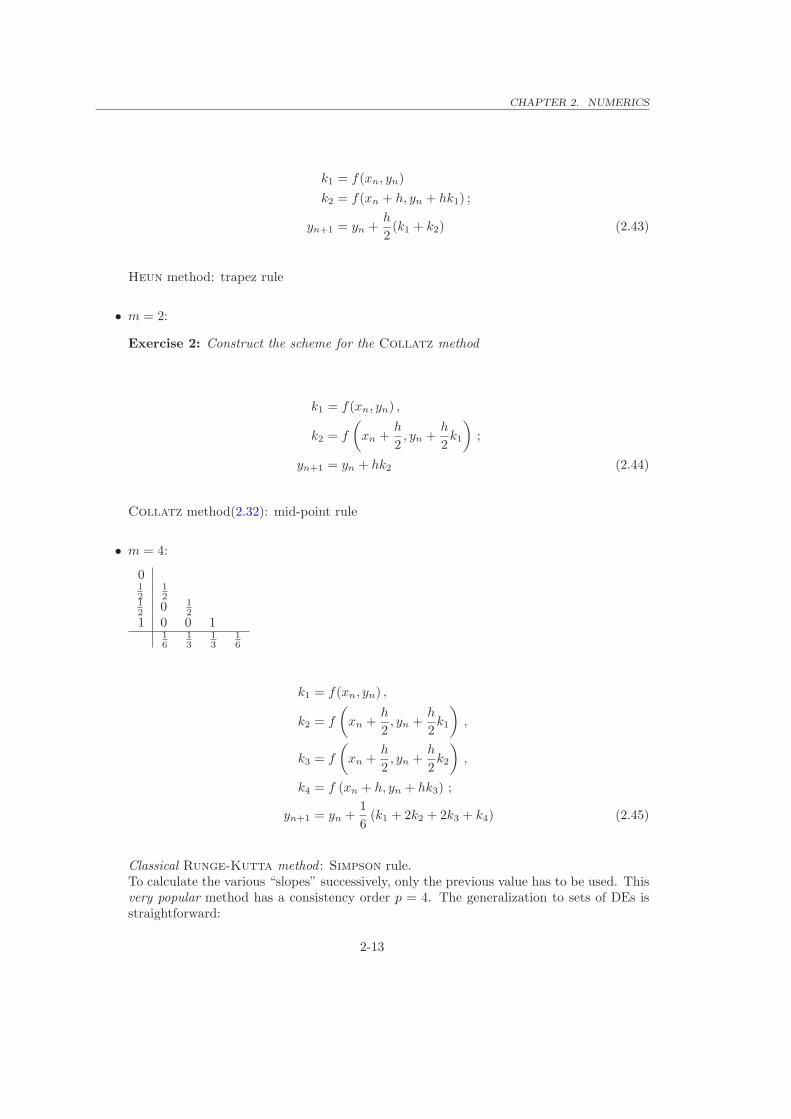
k1 = f(xn, yn)
k2 = f(xn + h, yn + hk1) ;
yn+1 = yn +h
2(k1 + k2) (2.43)
Heun method: trapez rule
• m = 2:
Exercise 2: Construct the scheme for the Collatz method
k1 = f(xn, yn) ,
k2 = f
(
xn +h
2, yn +
h
2k1
)
;
yn+1 = yn + hk2 (2.44)
Collatz method(2.32): mid-point rule
• m = 4:
012
12
12 0 1
21 0 0 1
16
13
13
16
k1 = f(xn, yn) ,
k2 = f
(
xn +h
2, yn +
h
2k1
)
,
k3 = f
(
xn +h
2, yn +
h
2k2
)
,
k4 = f (xn + h, yn + hk3) ;
yn+1 = yn +1
6(k1 + 2k2 + 2k3 + k4) (2.45)
Classical Runge-Kutta method : Simpson rule.To calculate the various “slopes” successively, only the previous value has to be used. Thisvery popular method has a consistency order p = 4. The generalization to sets of DEs isstraightforward:
2-13
CHAPTER 2. NUMERICS
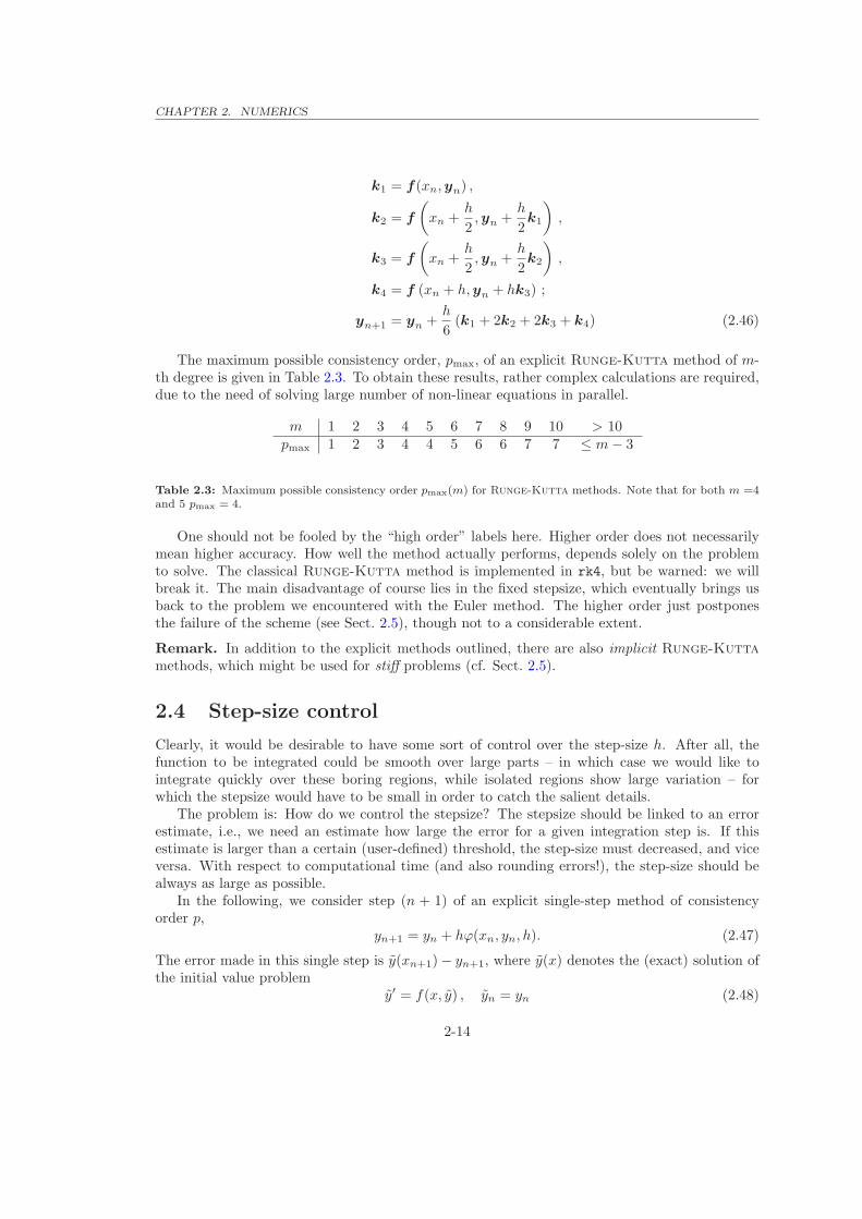
k1 = f(xn,yn) ,
k2 = f
(
xn +h
2,yn +
h
2k1
)
,
k3 = f
(
xn +h
2,yn +
h
2k2
)
,
k4 = f (xn + h,yn + hk3) ;
yn+1 = yn +h
6(k1 + 2k2 + 2k3 + k4) (2.46)
The maximum possible consistency order, pmax, of an explicit Runge-Kutta method of m-th degree is given in Table 2.3. To obtain these results, rather complex calculations are required,due to the need of solving large number of non-linear equations in parallel.
m 1 2 3 4 5 6 7 8 9 10 > 10pmax 1 2 3 4 4 5 6 6 7 7 ≤ m − 3
Table 2.3: Maximum possible consistency order pmax(m) for Runge-Kutta methods. Note that for both m =4and 5 pmax = 4.
One should not be fooled by the “high order” labels here. Higher order does not necessarilymean higher accuracy. How well the method actually performs, depends solely on the problemto solve. The classical Runge-Kutta method is implemented in rk4, but be warned: we willbreak it. The main disadvantage of course lies in the fixed stepsize, which eventually brings usback to the problem we encountered with the Euler method. The higher order just postponesthe failure of the scheme (see Sect. 2.5), though not to a considerable extent.
Remark. In addition to the explicit methods outlined, there are also implicit Runge-Kuttamethods, which might be used for stiff problems (cf. Sect. 2.5).
2.4 Step-size control
Clearly, it would be desirable to have some sort of control over the step-size h. After all, thefunction to be integrated could be smooth over large parts – in which case we would like tointegrate quickly over these boring regions, while isolated regions show large variation – forwhich the stepsize would have to be small in order to catch the salient details.
The problem is: How do we control the stepsize? The stepsize should be linked to an errorestimate, i.e., we need an estimate how large the error for a given integration step is. If thisestimate is larger than a certain (user-defined) threshold, the step-size must decreased, and viceversa. With respect to computational time (and also rounding errors!), the step-size should bealways as large as possible.
In the following, we consider step (n + 1) of an explicit single-step method of consistencyorder p,
yn+1 = yn + hϕ(xn, yn, h). (2.47)
The error made in this single step is y(xn+1)− yn+1, where y(x) denotes the (exact) solution ofthe initial value problem
y′ = f(x, y) , yn = yn (2.48)
2-14
CHAPTER 2. NUMERICS
The step-size shall be chosen such that this local error is constrained by
|y(xn+1) − yn+1| <∼ ∆0, (2.49)
where ∆0 > 0 is a given tolerance level. Since y(xn+1) is unknown, the error has to be estimated.In our case, the local discretization error
ln+1 := y(xn+1) − y(xn)︸ ︷︷ ︸
=yn
−hnϕ(xn, y(xn)︸ ︷︷ ︸
=yn
, hn) (2.50)
with y(x) instead of y(x) is equal to the corresponding global discretization error
gn+1 := y(xn+1) − yn+1, (2.51)
and because of our assumptions we have (convergence provided)
gn+1 = ln+1 ≈ chp+1n . (2.52)
2.4.1 Error estimate from step doubling
Originally, the error estimate was achieved by step doubling. The integration step is performedtwice, once with the full step-size, then, independently, twice with the half step-size. For a stepwith step-size hn, we have from above
g(1)n+1 = y(xn+1) − y
(1)n+1 ≈ chp+1
n , (2.53)
whereas a double-step with size hn
2 results in
g(2)n+1 = y(xn+1) − y
(2)n+1 ≈ 2c
(hn
2
)p+1
≈ chp+1
n
2p(2.54)
(remember that c is independent of h). Subtracting (2.54) from (2.53) yields
y(2)n+1 − y
(1)n+1 ≈
(1 − 2−p
)chp+1
n . (2.55)
2.9 Example. For a Runge-Kutta method of order p = 4, this difference (in terms of step-size hn/2) is givenby
y(2)n+1 − y
(1)n+1 ≈ 30 c
` hn
2
´5(2.56)
A final combination again with (2.53) results in
y(xn+1) − y(1)n+1 ≈ chp+1
n ≈y(2)n+1 − y
(1)n+1
1 − 2−p. (2.57)
Optimum step-size. Let hn be the step-size which should result in the predefined tolerancelevel,
∣∣y(xn + hn) − yn+1
∣∣ = ∆0. (2.58)
From (2.52) we have
∆0 ≈ |c| hp+1n , (2.59)
2-15
CHAPTER 2. NUMERICS
and from (2.57) and (2.59) we obtain
hn ≈ hn
(1 − 2−p) ∆0∣∣∣y
(2)n+1 − y
(1)n+1
∣∣∣
1/(p+1)
≈ hn
(∆0
|∆y|
)1/(p+1)
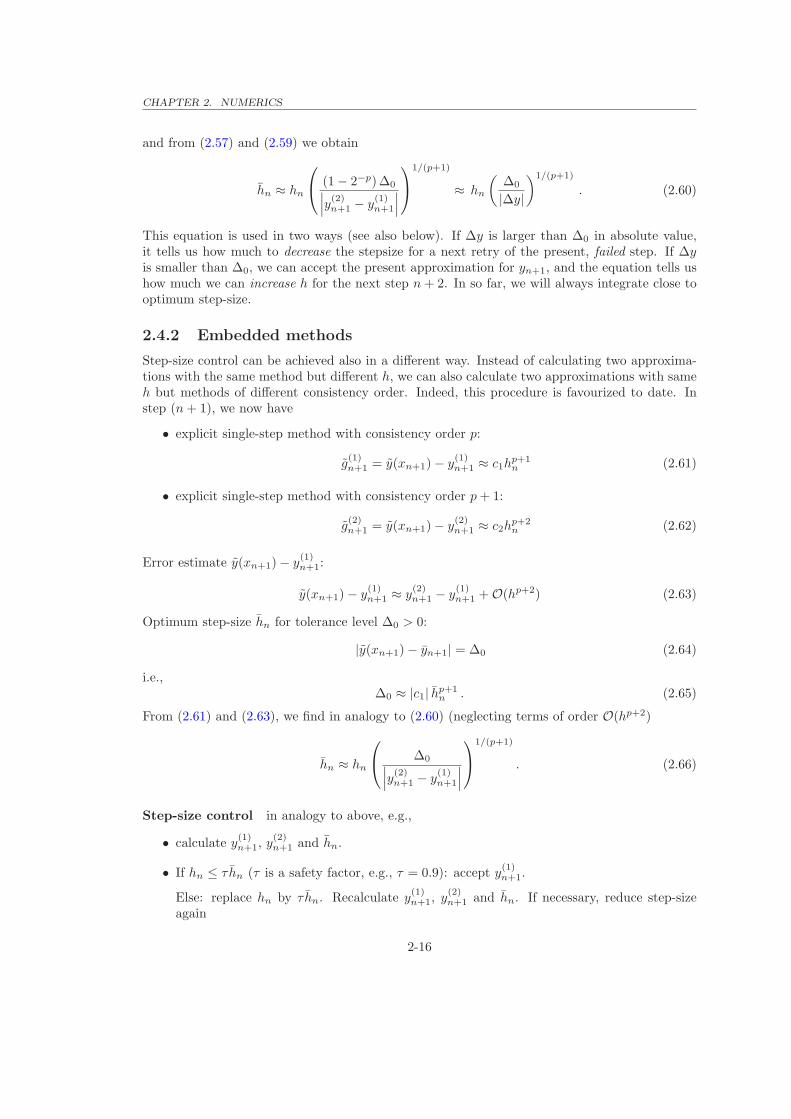
. (2.60)
This equation is used in two ways (see also below). If ∆y is larger than ∆0 in absolute value,it tells us how much to decrease the stepsize for a next retry of the present, failed step. If ∆yis smaller than ∆0, we can accept the present approximation for yn+1, and the equation tells ushow much we can increase h for the next step n + 2. In so far, we will always integrate close tooptimum step-size.
2.4.2 Embedded methods
Step-size control can be achieved also in a different way. Instead of calculating two approxima-tions with the same method but different h, we can also calculate two approximations with sameh but methods of different consistency order. Indeed, this procedure is favourized to date. Instep (n + 1), we now have
• explicit single-step method with consistency order p:
g(1)n+1 = y(xn+1) − y
(1)n+1 ≈ c1h
p+1n (2.61)
• explicit single-step method with consistency order p + 1:
g(2)n+1 = y(xn+1) − y
(2)n+1 ≈ c2h
p+2n (2.62)
Error estimate y(xn+1) − y(1)n+1:
y(xn+1) − y(1)n+1 ≈ y
(2)n+1 − y
(1)n+1 + O(hp+2) (2.63)
Optimum step-size hn for tolerance level ∆0 > 0:
|y(xn+1) − yn+1| = ∆0 (2.64)
i.e.,∆0 ≈ |c1| h
p+1n . (2.65)
From (2.61) and (2.63), we find in analogy to (2.60) (neglecting terms of order O(hp+2)
hn ≈ hn
∆0
∣∣∣y
(2)n+1 − y
(1)n+1
∣∣∣
1/(p+1)
. (2.66)
Step-size control in analogy to above, e.g.,
• calculate y(1)n+1, y
(2)n+1 and hn.
• If hn ≤ τ hn (τ is a safety factor, e.g., τ = 0.9): accept y(1)n+1.
Else: replace hn by τ hn. Recalculate y(1)n+1, y
(2)n+1 and hn. If necessary, reduce step-size
again
2-16

CHAPTER 2. NUMERICS
• Use τ hn as initial step-size for next step.
y(2)n+1 should be calculated in parallel to y
(1)n+1 with almost no additional effort. This can
be achieved by so-called embedded Runge-Kutta schemes, or Runge-Kutta-Fehlberg inte-grators. Fehlberg used the fact that for RK schemes of order p > 4, more than p functionevaluations are needed (though never more than p + 3, cf. Table 2.3). Fehlberg found a 5thorder method with m = 6 function evaluations, while another combination of those six functions(i.e., identical αr and βrs but different γr) yields a 4th order method. Thus, the method oflower order is embedded into the higher order one. Table 2.4 shows the coefficients for such ap = 4, 5 method with coefficients as derived by Cash & Karp, which are somewhat advantageouscompared to the original coefficients from Fehlberg.
015
15
310
340
940
35
310 − 9
1065
1 − 1154
52 − 70
273527
78
163155296
175512
57513824
44275110592
2534096
37378 0 250
621125594 0 512
1771 order 4
282527648 0 18575
483841352555296
27714336
14 order 5
Table 2.4: Embedded Runge-Kutta method with Cash/Karp coefficients, as used in subroutine rkck
2.4.3 Defining the tolerance level
With all this, at least the structure is set up. However, one question remains: How do we definethe tolerance level, ∆0, especially if we have a system of ODEs? This depends on the application.A first guess would be to choose a fractional error. However, this is bound to fail if we integrateoscillating functions, or simply quantities which are not positive definite (like, e.g., velocities!).So, should we use absolute errors? But then imagine you plan to integrate the trajectory ofa particle in a gravitational field of a star, let’s say. If the error in the radial coordinate r isabsolute, the integration will get less and less accurate the closer to the star the particle passes.One possibility is to use a scaling array with an entry for each ODE, such that for a fractionalerror ǫ, the ith equation would get a desired accuracy of
∆0 = ǫyscal,i, (2.67)
where yscal,i is set to yi for fractional errors, and to some absolute value for absolute errors. Auseful ”trick” to obtain constant fractional errors except near zero crossings is
yscal,i = |yi| + |h∂xyi|. (2.68)
2-17

CHAPTER 2. NUMERICS
This error scaling is done by the routine odeint.
2.5 Absolute Stability. Stiff sets of differential equations
Inappropriate use of numerical methods for solving initial value problems can lead to instabilities.In the following, we will discuss how to avoid them. Let us firstly consider the test initial valueproblem
y′ = λy, y(0) = 1, (2.69)
which has, for ℜ(λ) < 0 (denoting by ℜ the real part), the well known solution
y(x) = eλx. (2.70)
Let us solve this problem with the classical Runge-Kutta method (siehe (2.45)):
k1 = λyn,
k2 = λ
(
yn +h
2k1
)
,
k3 = λ
(
yn +h
2k2
)
,
k4 = λ (yn + hk3) ;
yn+1 = yn +h
6(k1 + 2k2 + 2k3 + k4) . (2.71)
Thus, we have
yn+1 = F (λh)yn (2.72)
with
F (λh) = 1 + λh +λ2h2
2+
λ3h3
6+
λ4h4
24. (2.73)
The exact solution, on the other hand, follows
y(xn+1) = eλhy(xn). (2.74)
Obviously, a 4th order Taylor expansion of eλh im λh recovers the factor F (λh). This isconsistent with the fact that the local discretization error is of O(h5).
The exact solution always decays with |y(x)| → 0 for x → ∞. The numerical approximation,in contrast, decays only (yn → 0 fur n → ∞) if
|F (λh)| < 1 (2.75)
Because of |F (λh)| → ∞ for ℜ(λ)h → −∞, this is not fulfilled for all λh. But for sufficientlysmall h, the condition (2.75) is warrented though.The set
µ ∈ C| |F (µ)| < 1
is called the region of absolute stability of the method. A measure for its size is the so-called
stability interval := stability region ∩ real axis.
2-18
CHAPTER 2. NUMERICS
1
1
−3 −2 0−1
−2
−3
−1
2
3
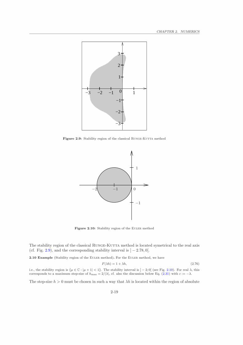
Figure 2.9: Stability region of the classical Runge-Kutta method
−2 −1
−1
0
1
Figure 2.10: Stability region of the Euler method
The stability region of the classical Runge-Kutta method is located symetrical to the real axis(cf. Fig. 2.9), and the corresponding stability interval is ] − 2.78, 0[.
2.10 Example (Stability region of the Euler method). For the Euler method, we have
F (λh) = 1 + λh, (2.76)
i.e., the stability region is µ ∈ C : |µ + 1| < 1. The stability interval is ] − 2; 0[ (see Fig. 2.10). For real λ, thiscorresponds to a maximum step-size of hmax = 2/|λ|, cf. also the discussion below Eq. (2.31) with c := −λ.
The step-size h > 0 must be chosen in such a way that λh is located within the region of absolute
2-19
CHAPTER 2. NUMERICS
stability. Otherwise, the method will give incorrect results and might even “explode”.If the region of absolute stability comprises the complete half-plane ℜ(µ) < 0, the method is
called absolutely stable.
Remark. Implicit Runge-Kutta methods are absolutely stable, whereas typical multi-stepmethods have a finite stability region.
Solutions of sets of differential equations, which describe physical (or chemical or biological)processes, often have the property that they exponentially reach a stationary solution, partlycoupled with (damped) oscillations (e.g., transient phenomena). The individual components ofthe solution can reach their final, constant value with different speed. This is typical for, e.g.,chemical reaction networks (molecule formation).
To solve such sets with not too small step-sizes, one has to use methods which are eitherabsolutely stable or at least have a large region of absolute stability. For an illustration, weconsider the test problem
y′ = Ay + b, y(x0) = y0 (2.77)
with a d × d matrix A with eigenvalues λi (i = 1, . . . , d) which all have a negative real part.If these real parts differ considerably, the initial value problem is called stiff. A measure for
the stiffness is the so called stiffness coefficient
S :=maxi |ℜ(λi)|
mini |ℜ(λi)|(2.78)
If the coefficients of the ODE (i.e., the matrix elements) comprise several orders of magnitude,S can reach values of O(106) or even more. To obtain meaningful numerical solutions, allproducts hλi have to be located in the region of absolute stability.
2.11 Example.0
@
y′
1y′
2y′
3
1
A =
0
@
−21 19 −2019 −21 2040 −40 −40
1
A
0
@
y1
y2
y3
1
A ,
0
@
y1(0)y2(0)y3(0)
1
A =
0
@
10−1
1
A (2.79)
The exact solution is0
@
y1(x)y2(x)y3(x)
1
A =
0
@
12e−2x + 1
2(cos(40x) + sin(40x)) e−40x
12e−2x − 1
2(cos(40x) + sin(40x)) e−40x
− (cos(40x) − sin(40x)) e−40x
1
A . (2.80)
Numerical solution with Euler method: initial value (y1(0.1), y2(0.1), y3(0.1))⊺ for xstart = 0.1, step-size 0.04.The result is displayed in Fig. 2.11. The approximations at the end of the displayed interval are no longeracceptable, and the situation becomes even worse, if we consider the larger interval from 0.1 to 1.0 in Fig. 2.12(note the different scale).
Since the eigenvalues of matrix A (2.79) are λ1 = −2, λ2 = −40 + 40i and λ3 = −40 − 40i, the stiffnesscoefficient is S = 20, i.e., the problem is not particularly stiff. With a step-size of h = 0.04 the producthλ1 = −0.08 is located within the stability region µ ∈ C : |µ + 1| < 1 of the Euler method (cf. Fig. 2.10),whilst hλ2 = −1.6 + 1.6i and hλ3 = −1.6 − 1.6i are located outside. Thus, the strong deviation of the numericalsolution from the exact one is due to the violation of the stability condition by eigenvalues λ2 and λ3, although
their contribution to the solution almost vanished for x >∼ 0.1. In order that all products hλi, i = 1, 3 are locatedwithin the stability region, the step-size must be h < 0.025. In this case then, the numerical solution is satisfactory.
An alternative approach to derive the stability condition for the Euler-method is as follows.We consider a set of ODEs
y′ = A · y (2.81)
where A is a real matrix with eigenvalues λi (i = 1, . . . , d) which all have a negative real part (inorder to assure that the exact solutions are exponentially decaying). Explicit differencing (see2.31) gives
yn+1 = (1 + Ah) · yn
= C · yn
(2.82)
2-20

CHAPTER 2. NUMERICS
y1(x)
y2(x)
y3(x)
approximations for y1(x)
approximations for y2(x)
approximations for y3(x)
−1
0
0
1
0.1 0.2 0.3
Figure 2.11: Analytical and numerical solution of example 2.11 for small x-values
0
0.1 0.5 1.0
−1000
1000
2000
3000
Figure 2.12: As Fig. 2.11, but for larger x-values
Now, a matrix Cn → 0 only if the absolutely largest eigenvalue |λmax| < 1. Let us denote theeigenvalues of A by µi = −ci + iℑi, where ci > 0 and ℑi is the imaginary part of µi. Thus, theeigenvalues of C are (1 − cih + iℑi h) and the maximum step-size follows as
hmax <2
max(ci +ℑ2
i
ci
)(2.83)
2-21
CHAPTER 2. NUMERICS
Exercise 3: Prove Eq. (2.83) and show that the maximum step-size in example 2.11 indeed ishmax = 0.025.
Implicit differencing evaluates the RHS of the ODE not at position n, but n + 1, i.e.
yn+1 = yn + hy′n+1 (2.84)
which is equivalent toyn+1 = (1 − Ah)−1 · y
n(2.85)
If we denote the eigenvalues of A as above, the eigenvalues of (1−Ah)−1 are (1+cih− iℑi h)−1,and their absolute value is < 1 ∀h. Thus, the implicit scheme is stable for all step-sizes h (andfor the example above, it converges to the correct solution even for very large h). The downsideis that each integration step requires a matrix inversion, and that the accuracy (for small x) israther low, if h is signficantly larger than in the corresponding explicit scheme.
2.6 Semi-implicit methods
Since by far not all ODEs have linear coefficiencts (the matrix A above), we need to generalizethe implicit method for ODEs:
y′ = f(y) → yn+1 = yn + hf(yn+1) (2.86)
Generally, this set of equations needs to be solved iteratively at each timestep, which in mostcases means a prohibitively large computational effort. A way out is to linearize the equations,i.e.
yn+1 = yn + h
(
f(yn) +∂f
∂y|y
n· (yn+1 − yn)
)
(2.87)
Here ∂f/∂y is the Jacobian matrix of partial derivatives of the ODE’s RHS w.r.t yi, i.e.
∂f
∂y≡
∂f1
∂y1
∂f1
∂y2· · · ∂f1
∂yn
∂f2
∂y1
∂f2
∂y2· · · ∂f2
∂yn
· · · · · · · · · · · ·
∂fn
∂y1
∂fn
∂y2· · · ∂fn
∂yn
(2.88)
Eq. [2.87] can be rearranged as
yn+1 = yn + h
(
1 − h∂f
∂y
)−1
· f(yn) (2.89)
If h is not too big, usually one iteration of Newton’s method is enough. This means that ateach step we have to invert the matrix 1 − h∂f/∂y to find yn+1. Since the derivative (dueto the linearization) is taken at yn, the method is called a semi-implicit Euler method. It isnot guaranteed to be stable, but it usually is, since the Jacobian locally corresponds to theconstant matrix A from above. Of course, eq. [2.89] is only 1st order (as the explicit Eulerintegrator eq. [2.31]). Again, going to higher order (and subsequently higher computationaleffort) in most cases pays off, since generally fewer steps are needed. The most common methods
2-22
CHAPTER 2. NUMERICS
are (a) generalized RK-schemes (Rosenbrock), an example of which has been implementedin subroutine stiff, (b) generalized Burlisch-Stoer methods 2 (extrapolation methods), seePress et al. (1992), and (c) predictor-corrector methods.
The Rosenbrock methods are close to the embedded Runge-Kutta-Fehlberg integrator intro-duced in Sect. 2.4.2. They are robust and perform well for accuracies of ǫ ≈ 10−4 · · · 10−5 andfor systems of up to approximately 10 ODEs. For larger systems or higher accuracies, the morecomplicated alternatives mentioned above are preferrable.
A Rosenbrock method seeks a solution of the form
y(x0 + h) = y0 +s∑
i=1
ciki (2.90)
where the corrections ki are found by solving s linear equations that generalize the structure ineq. [2.89]:
(1 − γh∂f
∂y) · ki = hf(y0 +
i−1∑
j=1
αijkj) + h∂f
∂y·
i−1∑
j=1
γijkj i = 1, · · · , s (2.91)
The coefficients (γ, ci, αij , γij) are fixed constants independent of the problem. For γ = γij = 0the scheme reverts to an explicit RK-scheme. Eq. [2.91] can be solved successively for ki. Again,as above, we are interested in the adaptive stepsize control, and – again again – there exists anembedded scheme which returns solutions accurate to 4th and 3rd order (compared to 5th and4th order previously) by using the same function evaluations with different coefficients.
The details of the scheme are of lesser interest here, however, one point should be raised. Asbefore, the choice of the “correct” (i.e. most appropriate) error criterion is crucial. This evenmore so here, because of the stiff nature of the ODEs, since they often have pieces of the solutionthat decay strongly and aren’t of interest, so it wouldn’t make any sense to assign them the sameaccuracy (and spend lots of time on that) as to the “relevant” solution parts. Obviously, thesechoices depend on the problem. One might control the relative error above some threshold Cand the absolute error below the threshold by setting (cf. Sect. 2.4.3)
yscal = max(C, |y|) (2.92)
If the variables are properly non-dimensionalized, the components of C should be of order unity,which should be used as a default value as well.
2conventional Burlisch-Stoer integrators are very useful for integrating non-stiff problems, which have arather smooth function f(x, y). The method is similar to the Romberg integration, i.e., involves an extrapolationto stepsize zero.
2-23

CHAPTER 2. NUMERICS
2-24
Chapter 3
Physics – Cosmological Models
In this chapter, we will give a brief introduction into the derivation and some simple appli-cations of cosmological models. In particular, we will consider the Friedmann-Lemaıtremodels which decribe (in form of an initial value problem) the temporal evolution of the so-called cosmic scale, R(t). Solutions for the behaviour of R(t), in dependence of various en-ergy density terms (matter, radiation, “vacuum”/dark energy), will be obtained by numericalmethods on the second day of our numerical lab work. There is a vast number of literaturecovering the corresponding physics (cited, e.g., in Wilms05), where, to some extent, we willfollow the text book by Roos (2003). Note that we have included a useful manuscript intothe course material provided, following a lecture given by J. Wilms (University Tubingen 2005,http://astro.uni-tuebingen.de/∼wilms/teach/cosmo/index.html). This manuscript willbe cited as “Wilms05” in the following.1
3.1 Cosmological redshift and Hubble’s law
In 1929, E. Hubble discovered that the spectral lines emitted from various galaxies of well-knowndistances are systematically redshifted, by wavelength shifts
λobs = λemit(1 + z) or z =∆λ
λ=
λobs − λemit
λemit. (3.1)
Interpreted in terms of a recession-velocity,
v
c:= z =
∆λ
λ, (3.2)
and combining his measurements with the distances of the line-emitting galaxies, Hubble sug-gested these redshifts to be a linear function of distance,
c z = v = H0r. (3.3)
This relation is meanwhile called Hubble’s law, with Hubble parameter2 H0, where the sub-script “0” refers to our present time, t0. From the relatively close galaxies studied by Hubble,he could only determine a linear relation, though higher order terms in r cannot be excluded
1Be prepared for a couple of typos in this script, which have been (hopefully) corrected here.2The alternative denotation as Hubble’s constant is somewhat misleading, since the quantity itself is changing
with time.
3-1
CHAPTER 3. PHYSICS – COSMOLOGICAL MODELS
and are present indeed (see Eq. 3.85). The message of this law is that the Universe is expanding,and from the so-called cosmological principle (i.e., the Universe is assumed to be homogeneousand isotropic on large scales), it can be shown that observers located at different positions wouldalways measure such a law: independent from location, astronomical objects recede from theobserver at the same rate. Thus, a homogeneous and isotropic universe does not have a center.
With respect to redshift alone, the Hubble law reads,
z = H0r
c(3.4)
and the inverse of H0 has the dimensions of a time, which gives a characteristic timescale for theexpansion of the Universe (though not necessarily its actual age), which is called the Hubbletime,
τH = H−10 = h−1 × 9.78 · 109 yr, (3.5)
where h is a dimensionless quantity, conveniently defined as
h = H0/(100 km s−1 Mpc−1). (3.6)
Present measurements can restrict h quite precisely, h ≈ 0.73 ± 0.05, though there is a certainpossibility that its value might be smaller by roughly 15%.
Though the actual size of our Universe is “unmeasurable”, one usually describes distances atdifferent epochs (which will change due to the expansion or contraction) in terms of a cosmicscale R(t) (see below), and its present value is denoted by R0 = R(t0). Additionally, one cannormalize R(t) by its present value and define a cosmic scale factor,
a(t) := R(t)/R0. (3.7)
This scale factor affects all distances, in particular also the wavelength λemit emitted at time tand observed as λobs at t0,
λemit
R(t)=
λobs
R0. (3.8)
Indeed, this relation can be simply derived from the Robertson-Walker metric (see Sect. 3.3),accounting for the fact that for photons ds2 = 0 and that comoving distances (in this case, thosetraveled by photons) remain preserved in such a metric (see Wilms05, p. 4-19).
By a Taylor expansion of a(t) for t < t0, we find to first order
a(t) = a(t0) −∂a
∂t|t0 (t0 − t) = 1 − a0 (t0 − t). (3.9)
With source distance r = c (t0 − t) and
λobs
λemit=
R0
R(t)= a−1, (3.10)
the redshift can be expressed as
z =λobs
λemit− 1 = a−1 − 1 ≈
1
1 − a0 (t0 − t)− 1 ≈ a0 (t0 − t) = a0
r
c. (3.11)
Thus, both redshift and Hubble parameter are related to the cosmic scale factor
3-2
CHAPTER 3. PHYSICS – COSMOLOGICAL MODELS
1 + z =λobs
λemit=
1
a(t)(3.12)
a0 = a(t0) =R0
R0=
R(t0)
R(t0)= H0, (3.13)
i.e., H0 is nothing else than the present rate of change in this factor (since we know that H0 ispositive, we know that we have an expanding universe at present).
Remark1. From the above, it should be clear that the cosmological redshift is a consequence of theexpansion of the Universe and not of the velocities of the receding objects. There are, of course,such kinematic effects as well (e.g., peculiar velocities resulting from (gravitationally induced)flows on smaller scales such as the Virgo-centric flow), which have to be corrected for whenmeasuring the cosmological redshift.2. For distant objects (of the order of the Hubble radius rH = c/H0 ≈ 3000/h Mpc, i.e., forobjects which would recede from us with the speed of light according to the linear Hubble law),this law has to be modified for relativistic effects. Indeed, it turns out that the redshift fromobjects located at rH becomes infinite, i.e., we cannot obtain information from larger distances.
3.2 Newtonian expansion
One of the key questions in cosmology is whether the Universe as a whole is a gravitationallybound system in which the expansion will be halted one day. A simple model using Newtonionmechanics will give a first answer. Note already here that the following results can be derivedfrom General Relativity (GR) as well, in the limit of weak gravitational fields.
Consider a galaxy of gravitating mass mg located at distance r from the center of a sphereof mean mass density, ρ. The total mass of the sphere is
M =4π
3r3ρ, (3.14)
so that the gravitational potential of the galaxy is
U = −GMmg
r= −
4π
3Gmgρr2, (3.15)
with gravitational constant G. Thus, the acceleration of the galaxy towards the center of thesphere is given by
r = −GM
r2= −
4π
3Gρr, (3.16)
which is nothing else than Newton’s law. In a Universe expanding according to Hubble’s law,the galaxy has a kinetic energy of
T =1
2mv2 =
1
2m(H0r)
2, (3.17)
with inertial mass m. Using the equivalence principle (inertial = gravitating mass), m = mg,the total energy of the galaxy is
E = T + U =1
2m(H0r)
2 −4π
3Gmgρr2 = mr2(
1
2H2
0 −4π
3Gρ), (3.18)
3-3

CHAPTER 3. PHYSICS – COSMOLOGICAL MODELS
which immediately tells that the expansion will come to a halt (E ≤ 0) if the mass density insidethe sphere (i.e., the mean density of the Universe), ρ, is larger/equal than the critical density,
ρc =3H2
0
8πG. (3.19)
If ρ > ρc, we speak of a closed, otherwise of an open Universe. Note that ρc is the present criticaldensity, corresponding to the present Hubble parameter.Exercise 4: Calculate the critical density, in units of g/cm3 and with respect to h
Since distance and density are time-dependent, they change with the expansion. Denoting theirpresent (t = t0) values by subscript “0”, we have
r(t) = a(t) ∗ r0; ρ(t) = ρ0/a3(t) (3.20)
(mass conservation), and Newton’s law (3.16) yields
a =r
r0= −
4π
3G
r
r0
ρ
a3= −
4π
3Gρ0a
−2. (3.21)
Multiplying this equation on both sides with 2 a,
2aa = −8π
3Gρ0
a
a2, (3.22)
this is equivalent tod
daa2 =
8π
3Gρ0
d
da
(1
a
), (3.23)
which can be easily integrated from t0 to t (with a0 = 1)
a2(t) − a2(t0) =8π
3Gρ0
( 1
a(t)− 1). (3.24)
By introducing the density parameter
Ω0 =ρ0
ρc=
8πGρ0
3H20
(3.25)
(in this scenario, Ω0 = 1 would denote a Universe at critical density), we obtain
a2 = H20Ω0(
1
a− 1) + a2(t0) (3.26)
and, using the definition for H0 = a(t0)
a2
H20
= (1 − Ω0 +Ω0
a), (3.27)
which is identical with the (first) Friedmann equation for similar conditions (only matter, noradiation, no cosmological constant).
An “empty” universe (ρ0 = 0 = Ω0) would expand forever, with constant rate a = H0. Onthe other hand, a steady state universe would imply H0 = 0.
Since a2 ≥ 0 always, we must have
1 − Ω0 − Ω0/a ≥ 0
as well. This implies
3-4
CHAPTER 3. PHYSICS – COSMOLOGICAL MODELS
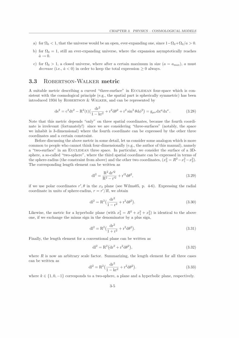
a) for Ω0 < 1, that the universe would be an open, ever-expanding one, since 1−Ω0+Ω0/a > 0.
b) for Ω0 = 1, still an ever-expanding universe, where the expansion asymptotically reachesa → 0.
c) for Ω0 > 1, a closed universe, where after a certain maximum in size (a = amax), a mustdecrease (i.e., a < 0) in order to keep the total expression ≥ 0 always.
3.3 Robertson-Walker metric
A suitable metric describing a curved “three-surface” in Euclidean four-space which is con-sistent with the cosmological principle (e.g., the spatial part is spherically symmetric) has beenintroduced 1934 by Robertson & Walker, and can be represented by
ds2 = c2dt2 − R2(t)( dr2
1 − kr2+ r2dθ2 + r2 sin2 θdφ2
)= gµνdxµdxν . (3.28)
Note that this metric depends “only” on three spatial coordinates, because the fourth coordi-nate is irrelevant (fortunately!) since we are considering “three-surfaces” (notably, the spacewe inhabit is 3-dimensional) where the fourth coordinate can be expressed by the other threecoordinates and a certain constraint.
Before discussing the above metric in some detail, let us consider some analogon which is morecommon to people who cannot think four-dimensionally (e.g., the author of this manual), namelya “two-surface” in an Euclidean three space. In particular, we consider the surface of a 3D-sphere, a so-called “two-sphere”, where the third spatial coordinate can be expressed in terms ofthe sphere-radius (the constraint from above) and the other two coordinates, (x2
3 = R2−x21−x2
2).The corresponding length element can be written as
dl2 =R2 dr′2
R2 − r′2+ r′2dθ2, (3.29)
if we use polar coordinates r′, θ in the x3 plane (see Wilms05, p. 4-6). Expressing the radialcoordinate in units of sphere-radius, r = r′/R, we obtain
dl2 = R2( dr2
1 − r2+ r2dθ2
). (3.30)
Likewise, the metric for a hyperbolic plane (with x23 = R2 + x2
1 + x22) is identical to the above
one, if we exchange the minus sign in the denominator by a plus sign,
dl2 = R2( dr2
1 + r2+ r2dθ2
). (3.31)
Finally, the length element for a conventional plane can be written as
dl2 = R2(dr2 + r2dθ2
), (3.32)
where R is now an arbitrary scale factor. Summarizing, the length element for all three casescan be written as
dl2 = R2( dr2
1 − kr2+ r2dθ2
). (3.33)
where k ∈ 1, 0,−1 corresponds to a two-sphere, a plane and a hyperbolic plane, respectively.
3-5

CHAPTER 3. PHYSICS – COSMOLOGICAL MODELS
In so far, the generalization to three-dimensional (hyper-)surfaces on four-dimensional spheres,i.e., three-spheres, flat three-space and three-hyperboloids is (almost) straightforward (thoughthe author still has a problem to imagine the first and the last case). By allowing the generalizedradius/scale factor to become time-dependent and by including the time coordinate into the met-ric (which is already required in special relativity), we finally obtain the Robertson-Walkermetric, Eq. 3.28.
Comparing the length element in the RW-metric with the corresponding tensor formulation,the components of gµν are given by (with x0 = ct)
g00 = 1, g11 = −R2
1 − kr2, g22 = −R2r2, g33 = −R2r2 sin2 θ (3.34)
where k ∈ 1, 0,−1 is called the curvature parameter and corresponds to the three geometriesoutlined above.
If the Universe is homogeneous and isotropic at a given time and follows the RW-metric, itwill always retain these features: A galaxy at coordinates (r, θ, φ) will always remain at thesecoordinates, only the scale R(t) (i.e., the scale of distances) will change with time. Since thespatial displacement is dr = dθ = dφ = 0, the metric equation reduces to ds2 = c2dt2, andthe corresponding frame is called the comoving frame. Distances in this frame (“comoving”distances, d, which depend only on the spatial coordinates) remain preserved under expansion,whereas “proper” distances, D(t) = dR(t), change with time.
Summary: The above metric defines an universal coordinate system tied to the expansion ofspace, whereas the scale R(t) describes its evolution.
3.4 Friedmann cosmologies
To obtain a model for an Universe which follows the cosmological principle, we have to combinethe RW metric with Einstein’s field equations,
Gµν =8πG
c4Tµν , (3.35)
where
Gµν = Rµν −1
2gµνR
is the Einstein tensor, derived from the Ricchi tensor Rµν and the Ricchi scalar R (not to beconfused with the cosmic scale!), where the Ricchi tensor itself is a contraction of the Riemanntensor Rαβγσ,
Rβγ = Rαβγα, R = gβγRβγ
and Tµν is the energy-stress tensor. One of the problems in GR is the calculation of the Riemanntensor (4th rank, i.e., 256 components, which mostly and fortunately are not independent orvanish), which itself is a combination of the so-called affine connections (in some languages,“Christoffel-symbols”) and their derivatives. The affine connections themselves (no tensors) arederivatives of the metric (here, we have the final relation to our work), and are required to allowfor a covariant formulation of the physical laws (i.e., formulations in terms of quantities whichremain invariant in arbitrary (e.g., accelerated) frames.)
To proceed further, we consider a comoving observer in a space decribed by the RW-metric.Under the assumption of the cosmological principle, the energy stress tensor becomes purely
3-6
CHAPTER 3. PHYSICS – COSMOLOGICAL MODELS
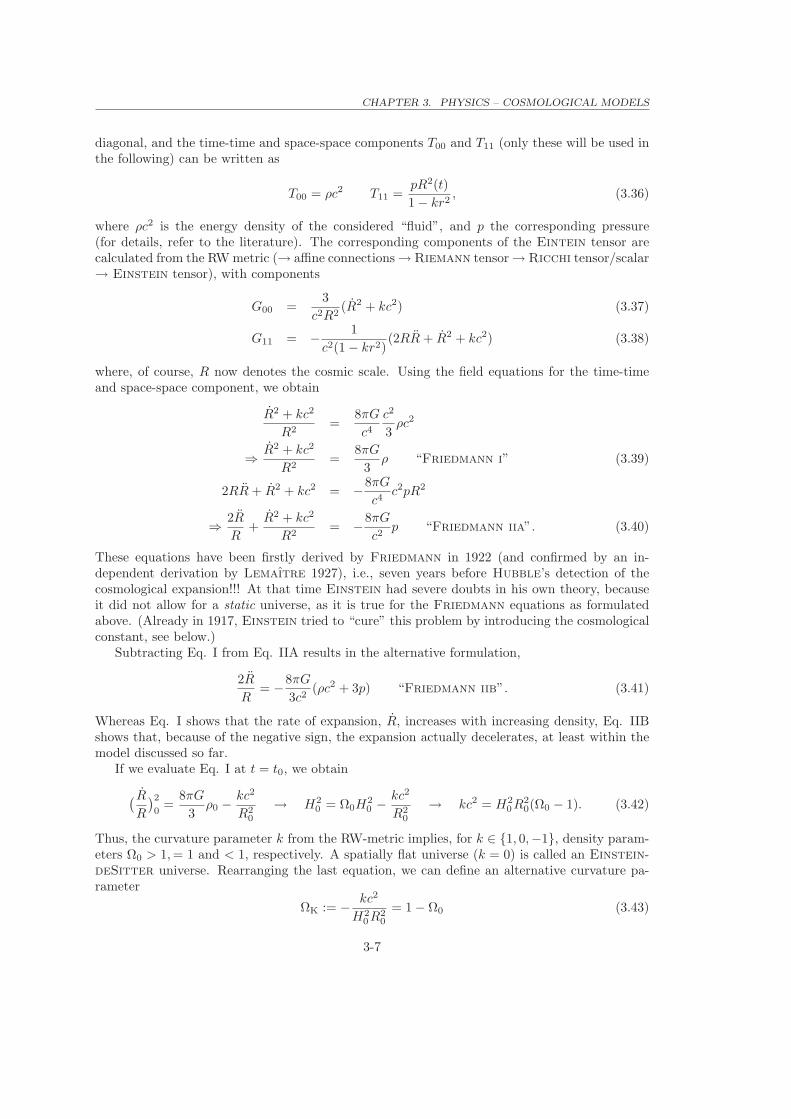
diagonal, and the time-time and space-space components T00 and T11 (only these will be used inthe following) can be written as
T00 = ρc2 T11 =pR2(t)
1 − kr2, (3.36)
where ρc2 is the energy density of the considered “fluid”, and p the corresponding pressure(for details, refer to the literature). The corresponding components of the Eintein tensor arecalculated from the RW metric (→ affine connections → Riemann tensor → Ricchi tensor/scalar→ Einstein tensor), with components
G00 =3
c2R2(R2 + kc2) (3.37)
G11 = −1
c2(1 − kr2)(2RR + R2 + kc2) (3.38)
where, of course, R now denotes the cosmic scale. Using the field equations for the time-timeand space-space component, we obtain
R2 + kc2
R2=
8πG
c4
c2
3ρc2
⇒R2 + kc2
R2=
8πG
3ρ “Friedmann i” (3.39)
2RR + R2 + kc2 = −8πG
c4c2pR2
⇒2R
R+
R2 + kc2
R2= −
8πG
c2p “Friedmann iia”. (3.40)
These equations have been firstly derived by Friedmann in 1922 (and confirmed by an in-dependent derivation by Lemaıtre 1927), i.e., seven years before Hubble’s detection of thecosmological expansion!!! At that time Einstein had severe doubts in his own theory, becauseit did not allow for a static universe, as it is true for the Friedmann equations as formulatedabove. (Already in 1917, Einstein tried to “cure” this problem by introducing the cosmologicalconstant, see below.)
Subtracting Eq. I from Eq. IIA results in the alternative formulation,
2R
R= −
8πG
3c2(ρc2 + 3p) “Friedmann iib”. (3.41)
Whereas Eq. I shows that the rate of expansion, R, increases with increasing density, Eq. IIBshows that, because of the negative sign, the expansion actually decelerates, at least within themodel discussed so far.
If we evaluate Eq. I at t = t0, we obtain
( R
R
)2
0=
8πG
3ρ0 −
kc2
R20
→ H20 = Ω0H
20 −
kc2
R20
→ kc2 = H20R2
0(Ω0 − 1). (3.42)
Thus, the curvature parameter k from the RW-metric implies, for k ∈ 1, 0,−1, density param-eters Ω0 > 1,= 1 and < 1, respectively. A spatially flat universe (k = 0) is called an Einstein-deSitter universe. Rearranging the last equation, we can define an alternative curvature pa-rameter
ΩK := −kc2
H20R2
0
= 1 − Ω0 (3.43)
3-7

CHAPTER 3. PHYSICS – COSMOLOGICAL MODELS
Let us indentify, for the moment, the density in Eq. I with mass-density alone, such that ρ(t) =ρ0/a3(t), similar to our examination of the Newtonian expansion (Sect. 3.2). Thus, for arbitraryt,
( R
R
)2=
8πG
3
ρ0
a3(t)−
kc2
R2. (3.44)
Multiplying by (R/R0)2 = a2(t), we obtain
a2 =8πG
3
ρ0
a3a2 −
kc2
R20
= H20Ω0
1
a−
kc2
R20
= H20Ω0
1
a+ (1 − Ω0)H
20 (from Eq. 3.43)
= H20 (
Ω0
a+ 1 − Ω0) (3.45)
which is identical with the result of the Newtonian approach, Eq. 3.27. Another interestingrelation follows from a somewhat different manipulation. Again, evaluate Eq. I at arbitrary t,
kc2 =8πG
3ρR2 − R2
= R2(8πG
3ρc(t)Ω(t) − (
R
R)2)
with ρc(t) =3H2(t)
8πG, Ω(t) =
ρ(t)
ρc(t), H(t) =
R
R
= R2(H2(t)Ω(t) − H2(t)
)= R2H2(t)
(Ω(t) − 1
). (3.46)
Equating this expression with the corresponding one from Eq. 3.42 (both being equal to theconstant term kc2),
R2H2(Ω − 1) = H20R2
0(Ω0 − 1)
a2H2(Ω − 1) = H20 (Ω0 − 1) →
Ω − 1
Ω0 − 1=
H20
H2a2=( R0
R
)2=( a0
a
)2≪ 1 for t/t0 ≪ 1, (3.47)
since a tends towards infinity for small t, as we will see later. From this condition then, Ω musthave been very close to unity, or, in other words, the early Universe must have been asymptoticallyflat! E.g., the maximum deviation from flatness during the phase of nucleosynthesis (t ≈ 1s) canbe constrained by <∼ 10−16, if the present day value of Ω0 is of the order of unity.
This is what is called the flatness problem. Had Ω been different from unity at its beginning,the Universe would have immediately recollapsed (within one Planck time), or expanded toofast to allow for the existence of mankind. Thus, the anthropocentric point of view requiresΩ = 1, i.e., k = 0. To generate a universe surviving for many Gigayears without Ω being exactlyunity would have required an incredible fine-tuning, which is extremely unlikely. Without goinginto details, inflation can cure this problem, by increasing the cosmological scale exponentially(factor of ≈ 1043) in a (very) early phase (t ≈ 10−34s) of the Universe (see below).
3-8
CHAPTER 3. PHYSICS – COSMOLOGICAL MODELS
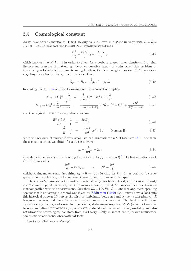
3.5 Cosmological constant
As we have already mentioned, Einstein originally believed in a static universe with R = R =0, R(t) = R0. In this case the Friedmann equations would read
kc2
R20
=8πG
3ρ0 = −
8πG
c2p0, (3.48)
which implies that a) k = 1 in order to allow for a positive present mass density and b) thatthe present pressure of matter, p0, becomes negative then. Einstein cured this problem byintroducing a Lorentz invariant term gµνλ, where the “cosmological constant”, λ, provides avery tiny correction to the geometry of space time:
Gµν := Rµν −1
2gµνR − gµνλ (3.49)
In analogy to Eq. 3.37 and the following ones, this correction implies
G00 → Gold00 −
λ
c2=
3
c2R2(R2 + kc2) − 3
λ
3c2(3.50)
G11 → Gold11 +
λ
c2
R2
1 − kr2= −
1
c2(1 − kr2)(2RR + R2 + kc2) +
λR2
c2(1 − kr2)(3.51)
and the original Friedmann equations become
R2 + kc2
R2−
λ
3=
8πG
3ρ (3.52)
R
R−
λ
3= −
4πG
3c2(ρc2 + 3p) (version B). (3.53)
Since the pressure of matter is very small, we can approximate p ≈ 0 (see Sect. 3.7), and fromthe second equation we obtain for a static universe
ρ0 =λ
4πG:= 2ρλ (3.54)
if we denote the density corresponding to the λ-term by ρλ = λ/(8πG).3 The first equation (withR = 0) then yields
kc2
R2= 8πGρλ → R2 =
kc2
λ(3.55)
which, again, makes sense (requiring ρ0 > 0 → λ > 0) only for k = 1. A positive λ curvesspace-time in such a way as to counteract gravity and to prevent a collapse!
Thus, a static universe with positive matter density has to be closed, and its mean densityand “radius” depend exclusively on λ. Remember, however, that “in our case” a static Universeis incompatible with the observational fact that H0 = (R/R)0 6= 0! Another argument speakingagainst static universes in general was given by Eddington (1930) (you might have a look intothis historical paper): If there is the slightest imbalance between ρ and λ (i.e., a disturbance), Rbecomes non-zero, and the universe will begin to expand or contract. This leads to still largerdeviations of ρ from λ, and so on. In other words, static universes are unstable (a fact not realizedbefore), and after Eddington’s paper Einstein abandoned his belief in this possibility and alsowithdraw the cosmological constant from his theory. Only in recent times, it was resurrectedagain, due to additional observational facts.
3previously called “vacuum density”
3-9

CHAPTER 3. PHYSICS – COSMOLOGICAL MODELS
3.6 Friedmann-Lemaıtre cosmologies
If the physics of the vacuum is Lorentz invariant4, i.e., looks the same to any inertial observer,its contribution to the energy-stress tensor is the same as Einstein’s correction λgµν to thegeometry, as noted by Lemaıtre. The content of Eqs. 3.52 and 3.53 does not change if the cor-responding terms are moved from the lhs to the rhs of the equations, though their interpretationchanges. If put on the rhs, they appear as the density (first) and pressure (second equation) ofan additional fluid (originally identified with the above vacuum), with
density ρλ =λ
8πGand pressure pλ = −ρλc2 :
R2 + kc2
R2=
8πG
3(ρ + ρλ) (3.56)
2R
R+
R2 + kc2
R2= −
8πG
c2(p + pλ) version A (3.57)
R
R= −
4πG
3c2[(ρ + ρλ)c2 + 3(p + pλ)] (version B). (3.58)
In this interpretation then, for λ > 0 the gravitational effect of this fluid is to counteract, via itsnegative(!) pressure, the gravitational pull of “ordinary” matter, eventually even leading to anacceleration of the scale factor, whereas a negative λ would correspond to an additional attractiveterm.
Cosmologies as described by (3.56 to 3.58) with positive λ are nowadays called Friedmann-Lemaıtre cosmologies. Since we have to deal with energy densities/pressures from differentsources, the total density parameter is split into the different contributions by matter (includingthe dark one), radiation and cosmological constant
Ω0 = ΩM + ΩR + ΩΛ (3.59)
with ΩR and ΩΛ defined in analogy to (3.25), i.e.,
ΩR =ρr
ρc, ΩΛ =
ρλ
ρc=
λ
8πGρc=
λ
3H20
. (3.60)
As you will see (and hopefully confirm) during your practical work, the present values of ΩM andΩΛ are quite similar, ΩM ≈ 0.3 and ΩΛ ≈ 0.7. In other words, the density corresponding to thecosmological constant, ρλ, must be of similar order than the present critical density, or, moreprecisely, ρλ ≈ 0.7ρc ≈ 0.7h2 × 1.88 · 10−29g/cm
3≈ 6.5 · 10−30g/cm
3.
The vacuum energy problem. Using simple quantum-mechanical arguments, it can beshown that the actual vacuum energy of the Universe should be MUCH larger: Rememberthat the ground-state energy of a quantum-mechanical oscillator is not zero by E0 = 1/2~ω. Thegeneralization to fields is (almost) straightforward. A relativistic field may be thought of as acollection of harmonic oscillators of all possible frequencies. A simple example is provided by ascalar field (e.g., a spinless boson) of mass m. For this system, the vacuum energy is simply asum of contributions
4assuming that the vacuum state of the Universe is not simply an empty space, but the ground state of somephysical theory, where this ground state should be independent of coordinate system.
3-10

CHAPTER 3. PHYSICS – COSMOLOGICAL MODELS
E0 =∑
i
1
2~ωi (3.61)
where the sum extends over all possible modes in the field, i.e., over all wavevectors k. The corre-sponding energy density E0/L3 = ρvacc
2 can be calculated from integrating over all wavenumberspresent in a box of Volume L3 with periodical boundary conditions (λn = 2π/kn = L/n, n =1, 2, . . .), and results in
ρvacc2 =
~c
16π2k4max, (3.62)
where kmax ≫ mc/~ is the maximum wavenumber present in the field. Following Carroll et al.(1992), we estimate kmax as the energy scale at which our confidence in the formalism nolonger holds. For example, it is widely believed that the “Planck energy” EP marks a pointwhere conventional field theory breaks down due to quantum gravitational effects. This energyroughly corresponds to the situation when the wavelength of a particle reaches its correspondingSchwarzschild radius. More precisely, the Planck-mass is defined as the mass of a particlefor which the Schwarzschild radius is equal to the Compton wavelength divided by π,
1
π
2π~
mc=
2Gm
c2→ mP =
√
~c
G, (3.63)
and the corresponding energy is the Planck-mass times c2. Choosing thus ~kmaxc = EP, weobtain
kmax =
√
c3
G~(3.64)
ρvac =c5
16π2G2~= 3.3 · 1091g/cm
3(3.65)
Thus, the ratio of the expected ρvac to the “observed value” ρλ is O(10120), which indeed is notsoooo small.
As in classical mechanics, the absolute value of the vacuum energy has no measurable effectin non-gravitational quantum field theorys. Roughly spoken, non-gravitational forces dependon potential gradients, i.e., constant terms do not contribute. In GR, however, gravitationcouples to all energies and momenta, which must include the energy of the vacuum: The onlymanifestation of vacuum energy will be through its gravitational influence. For a density ashigh as given by Eq. 3.65, this would mean a dramatic expansion of the Universe: the cosmicmicrowave background would have cooled below 3 K in the first 10−41 s after the Big Bang.
The maximum wavenumber corresponding to the “observed” value of ρλ would be kmax ≈413 cm−1 ≈ 0.008 eV, which is way too low, since QM has been tested to be valid at muchhigher energies, and the reality of a vacuum energy density has been quantitatively verified bythe Casimir effect.
In physical terms, then, the cosmological constant problem is this: There are independentcontributions to the vacuum energy density from the virtual fluctuations of each field (since thereis not only a single field but many more, due to the presence of different particle species) andfrom the potential energy of each field (and maybe even from a “real” cosmological constantitself). Each of these contributions should be much larger than ρλ, but they seem to combineto a very small value.5 Thus, this situation indicates that new, unknown physics must play adecisive role, nowadays called “dark energy” (which usually has an energy density and equationof state which varies through space-time).
5At least at the present epoch, keeping in mind that the inflationary phase of the Universe requires a ratherlarge value of λ in this very first phase.
3-11

CHAPTER 3. PHYSICS – COSMOLOGICAL MODELS
3.7 Energy conservation and equation of state
Differentiating (3.56) with respect to time and combining the result with (3.53) to cancel thesecond derivatives, we obtain a new equation for the evolution of the energy density
ρc2 + 3H(t)(ρc2 + p) = 0, (3.66)
which is valid for both the total energy density and pressure and for their individual components,if different energy “forms” are present (following different equations of state). Eq. (3.66), whichcan be interpreted as a local energy conservation law, shows that the local energy density ischanged by the expansion/contraction and by the corresponding volume work. This equation alsoclarifies the (at first glance somewhat puzzling) fact that a negative pressure - which in “normallife” is encountered as a pull - leads to a gravitational repulsion, i.e., increased expansion: Thelarger the ratio of pressure to energy density, the more volume work is done, which has to becompensated by a faster decrease in available gravitating energy density. The lower the energydensity, however, the less the expansion (R2 ∝ (ρR)2)! For negative pressure, on the other hand,the volume “work” becomes a gain. Loosely formulated, we create energy from the expansionof space, and the decrease in available gravitating energy density is slower than for p > 0 (andstops completely for p = −ρc2). Consequently the expansion remains faster than for positivepressure. Note that a decelerating universe becomes an accelerating one if the dominating energydensities/pressures relate via p < −1/3ρc2.
By integration of Eq. 3.66 we obtain∫
ρ(t)
ρ(t) + p(t)/c2dt = −3
∫a(t)
a(t)dt, (3.67)
which can be immediately solved when the corresponding equation(s) of state is (are) known.
Equation of state (EOS). The most general form of an EOS in a space-time with RW metriccan be shown to be
p = wρc2 (3.68)
where w depends on the energy form considered. Assuming w to be constant with time, (3.67)results in
ρ(a) ∝ a−3(1+w) = (1 + z)3(1+w), (3.69)
because (1 + z) = a−1, cf. (3.12).
(i) For “ordinary” matter (in the spirit of cosmology, i.e., non-relativistic cold matter: pres-sureless, non-radiating dust and cold dark matter), we have p = 0 (otherwise, galaxieswould have random motions similar to that of gas particles under pressure which is notobserved), and thus w = 0. Accordingly,
ρm(a) = ρm(0)a−3. (3.70)
(ii) Radiation or relativistic hot gas composed of elastically scattering particles follows
pr =1
3εr =
1
3ρrc
2
(e.g., the ratio of 2nd moment of specific intensity, K, to mean intensity (0th moment), J ,is 1/3 for isotropic radiation). Thus, w = 1/3, and
ρr(a) = ρr(0)a−4. (3.71)
3-12

CHAPTER 3. PHYSICS – COSMOLOGICAL MODELS
(iii) As we have already seen, the pressure corresponding to a cosmological constant is pλ =−ρλc2, i.e., w = −1 and
ρλ(a) = ρλ(0) (3.72)
assuming that λ and w are constant over the considered expansion/contraction interval.This EOS can be derived from the energy-stress tensor of a perfect fluid required to beLorentz-invariant. Note that this follows also from the requirement that, under an adia-batic expansion/compression, ρvac should remain constant:
dQ = dU + pdV = ρvacc2dV + wρvacc
2dV!= 0 → w = −1
3.8 Evolution of the scale factor
We are now (finally!) ready to write down the “equation of motion” of the Universe, i.e., theevolution of the cosmic scale factor, a(t). By means of the above relations for the differentdensities, we obtain from the “first” Friedmann-Lemaıre equation (3.56)
R2 =8πG
3R2(ρm(0)
a3+
ρr(0)
a4+ ρλ
)− kc2, (3.73)
which can be easily rephrased in terms of the various density parameters,
a2 = a2H20
(ΩM
a3+
ΩR
a4+ ΩΛ +
ΩK
a2
)= H2
0
(ΩM
a+
ΩR
a2+ a2ΩΛ + ΩK
)(3.74)
again assuming λ to be constant. Convince yourself of the validity of this expression!
Remarks(i) You might ask yourself why we have always considered the two Friedmann(-Lemaıtre)equations throughout this chapter, when we finally use only the first one. Remember, however,that the 2nd equation has been used as well (together with the different equations of state) inorder to calculate the various densities as a function of a which otherwise would have remainedunspecified!(ii) Note also that the density parameters in (3.74) are defined with respect to the present criticaldensity (i.e., with respect to H0). The variation of the density parameters themselves can becalculated from Ω(t) = ρ(t)/ρc(t) and results in
ΩM(t) =H2
0
H2(t)
ΩM
a3, ΩR(t) =
H20
H2(t)
ΩR
a4, ΩΛ(t) =
H20
H2(t)ΩΛ, ΩK(t) =
H20
H2(t)
ΩK
a2.
Recall that the sum of the first three parameters must have been VERY close to unity for verysmall t. If λ indeed had been constant, the corresponding density parameter would have beennegligible at very early times, and radiation would have dominated throughout the very firstepochs.
At t = t0, a = H0 and a = 1 per definition, such that
H20 = H2
0
(ΩM + ΩR + ΩΛ + ΩK) or ΩK = 1 − (ΩM + ΩR + ΩΛ) = 1 − Ω0,
cf. Eq. 3.43. Thus, the evolution of the Hubble parameter follows
( a
a
)2= H(t) = H2
0
(1 − Ω0
a2+
ΩM
a3+
ΩR
a4+ ΩΛ
), (3.75)
During your practical work, you will solve this equation in the form
3-13
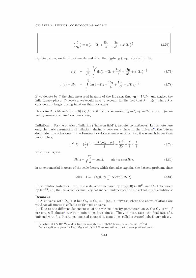
CHAPTER 3. PHYSICS – COSMOLOGICAL MODELS
( a
H0
)= ±
(1 − Ω0 +
ΩM
a+
ΩR
a2+ a2ΩΛ
) 12 . (3.76)
By integration, we find the time elapsed after the big-bang (requiring (a(0) = 0),
t(z) =1
H0
11+z∫
0
da(1 − Ω0 +
ΩM
a+
ΩR
a2+ a2ΩΛ
)− 12 (3.77)
t′(a) = H0t =
a∫
0
da(1 − Ω0 +
ΩM
a+
ΩR
a2+ a2ΩΛ
)− 12 (3.78)
if we denote by t′ the time measured in units of the Hubble-time τH = 1/H0, and neglect theinflationary phase. Otherwise, we would have to account for the fact that λ = λ(t), where λ isconsiderably larger during inflation than nowadays.
Exercise 5: Calculate t(z = 0) (a) for a flat universe consisting only of matter and (b) for anempty universe without vacuum energy.
Inflation. For the physics of inflation (“inflaton-field”), we refer to textbooks. Let us note hereonly the basic assumption of inflation: during a very early phase in the universe6, the λ-termdominated the other ones in the Friedmann-Lemaıtre equations (i.e., it was much larger thannow). Thus,
H2(t) =( a
a
)2=
8πG(ρm + ρr)
3−
kc2
R2+
λ
3≈
λ
3(3.79)
which results, via
H(t) =
√
λ
3= const, a(t) ∝ exp(Ht), (3.80)
in an exponential increase of the scale factor, which then also explains the flatness problem, since
Ω(t) − 1 = −ΩK(t) ∝1
a2∝ exp(−2Ht). (3.81)
If the inflation lasted for 100τH, the scale factor increased by exp(100) ≈ 1043, and Ω−1 decreasedby 10−86, i.e., the Universe became very flat indeed, independent of the actual initial conditions!
Remarks(i) A universe with ΩΛ > 0 but ΩM = ΩR = 0 (i.e., a universe where the above relations arevalid for all times) is called a deSitter universe.(ii) Due to the different dependencies of the various density parameters on a, the ΩΛ term, ifpresent, will almost7 always dominate at later times. Thus, in most cases the final fate of auniverse with λ > 0 is an exponential expansion, sometimes called a second inflationary phase.
6starting at t ≈ 10−34s and lasting for roughly 100 Hubble times (τH = 1/H ≈ 10−34s)7an exception is given for large ΩM and ΩΛ <∼ 0.2, as you will see during your practical work.
3-14
CHAPTER 3. PHYSICS – COSMOLOGICAL MODELS
Dark energy. An empirical approach to remove some of the problems with the cosmologicalconstant is to allow for a time-dependence, λ = λ(t). The corresponding energy component iscalled “dark energy” then. The initial conditions require a value corresponding to the expectedvacuum density, ρλ(tP) ≈ 10120ρλ(t0) at Planck-time tP = 10−47s, from which it decays to itspresent value, via matching the inflaton field as well. In this case, the EOS becomes (cf. 3.69)
pλ = −ρλ
(1 +
1
3
d ln ρλ(a)
d ln a
), (3.82)
which recovers the limit w = −1 for slowly changing ρλ. Of course, this approach does not tell usanything about the responsible physics. Note that enormous effort is presently spent to obtainobservational constraints on this EOS, which might allow to discriminate between competingphysical models or even trigger the set-up of new ones.
A popular model for dark energy is the so-called quintessence. Quintessence is a scalar fieldwhich has an equation of state with w < −1/3. As postulated above, quintessence is dynamic,and generally has a density and equation of state that varies through space-time.
Many models of quintessence have a so-called tracker behaviour, which partly solves thecosmological constant problem. In these models, the quintessence field has a density which closelytracks (but is less than) the radiation density until matter-radiation equality, which triggersquintessence to start having characteristics similar to the observed ρλ, eventually dominatingthe universe.
The deceleration parameter. In the beginning of this chapter, we derived Hubble’s lawfrom a linear expansion of the cosmic scale factor. Being familiar now with the Friedmann-Lemaıtre equations, we are also ready to perform a second order expansion, which will tell usabout the present acceleration or deceleration of the Universe:
R(t)
R0= a(t) ≈ a(t0) + H0(t − t0) +
1
2
R(t)
R0|t0 (t − t0)
2 (3.83)
where a(t0) = 1 and R can be extracted from the 2nd Friedmann-Lemaıtre equation. WithpM = 0 and neglecting ρλ, pλ for the moment, we find
R(t)
R(t)|t0 = −
4πG
3ρ0 = −
Ω0
2H2
0 (3.84)
a(t) = 1 + H0(t − t0) −1
2q0H
20 (t − t0)
2. (3.85)
In this expansion, the term
q0 := Ω0/2 = −R(t0)
R0H20
= −R(t0)R0
R2(t0)
measures the deceleration of the Universe (i.e., is positive for a decelerating cosmic scale).
Exercise 6: Generalize the above approach for ΩΛ 6= 0 but ΩR = 0 (which is legitimate at thepresent epoch). What can be concluded from a negative q0 as derived, e.g., from the distances ofSNe Ia?
3-15

CHAPTER 3. PHYSICS – COSMOLOGICAL MODELS
3-16
Chapter 4
Experiment
4.1 Numerical solution of ODEs: Test problems and inte-
grators
The problems covered in this section should be solved on the first day of our lab work.
4.1.1 The programs
Sources
Everything you need to edit, compile and run the codes (as well as to create the plots) canbe found in (sub-)directory codes. Switch to this directory, and have a look into the varioussubdirectories. All source-files (fortran 90, though with the ending .F) can be found indirectory src. A short structure of the program is given in frame.F.
In order not to (unintentionally) destroy or corrupt the original files, you will do most of thework in directory cmp. Switch to this directory, and have a look into the only file which shouldreside there, the Makefile. Check the various options, and install the source files in cmp.
Exercise 7: Locate all the sources and draw a diagram, specifying briefly what each subroutinedoes, down to the level of the integrators.
Compilation, execution and plotting
Compile all files using make (with the appropriate target).For all your following work, copy the resulting executable into directory run/problemX, where
X is a number 1. . . 4 corresponding to the specific test problem. Perform all runs (which usuallyrequires to update the particular input files) in this directory. Plots using idl have to be finallycreated in the directory plots, by using the plotting-routines to be found there.
4.1.2 Problem 1 – A first test
We will check whether the integrators are running smoothly by analytically and numericallysolving the ODE
∂xy(x) = a y(x) (4.1)
4-1
CHAPTER 4. EXPERIMENT
with a = 2.5 and the initial condition y(0) = 10−3 on the interval x = [0, 10].
Exercise 8: Solve Eq. (4.1) analytically :-).
Exercise P1: The integrators
All steps which are detailed in this exercise have to be performed analogously when working onthe other exercises.
P1.1: Obviously, something’s wrong with eulerstep.F: There’s nothing in there. That’s yourchance to write your version of an Euler integrator. Finalize the corresponding subroutine incmp, compile and copy the executable to run/problem1. Switch to the latter directory and testyour integrator using 100 steps. Before running the code, check the corresponding input fileframe.inp11 with respect to the various input quantities. Which ones are not needed to performthe Euler method?
In case, update those variables which are needed, and copy frame.inp11 to frame.inp, whichis the file being used by the executable. Hopefully, the program runs. Check now the created outputfile whether it makes sense!!!
Switch to plots. At first, study the first part of plotode.pro, regarding input, possiblekeywords and the variables runX/labelX, where X is 1. . . 4. Plot the result of your first test andthe analytical solution with plotode.pro and /points. Does the result agree with the analyticalsolution? Increase the number of steps to 1000. Don’t forget to change the “label” to‘00p1i2’ for the output file!. A correct label is important for the plotting routine to work!Gotten any better? (Plot the results of both simulations into one figure, and compare the results.)What are the mean relative errors?
After you are satified with your results, always create a corresponding .ps file (and, incase, a hardcopy) for your elaboration.
P1.2: Now use the 4th order RK integrator with 1000 steps. Again, choose a different ”label”(‘00p1i3’) to prevent overwriting of the previous result. Compare the result with the correspond-ing Euler and analytic solution (one plot, again with /points).
P1.3: Repeat P1.2 with rkqs and stiff. labels: ‘00p1i4’ and ‘00p1i5’. Convince yourselfthat the quantities eps etc in frame.inp make sense. How many integration steps does each ofthem need? Compare the required with the achieved accuracy. Are the more “fancy” integratorsmore accurate? What is their strength in this problem?
P1.4: Now use the RK integrator with adaptive step-size to find out the number of steps itneeds to actually obtain the same accuaracy as rk4 in 1000 steps. To this end, change the inputparameter eps as long as you have not obtained the desired accuracy. label: ‘00p1i6’.
P1.5: Summarize the results you obtained for Problem 1. Which integrator would you trustmost, and why?
4.1.3 Stiff Equations
As discussed above, physical systems which can be described by ODEs often evolve on verydisparate scales. Such a set of ODEs is called stiff. In the following, we will test the integratorson two different sets of stiff equations.
4-2
CHAPTER 4. EXPERIMENT
Problem 2 – Two coupled ODEs
We begin with the set
∂xy1 = 998y1 + 1998y2 (4.2)
∂xy2 = −999y1 − 1999y2 (4.3)
This corresponds to iprob = 2 in frame.inp. The initial conditions are y1(0) = 1 and y2(0) = 0,and the ODEs are to be integrated between x = [0, 4].
ADVANCED Exercise 9: Solve the above problem analytically. Remember the solution ansatzfor such homogeneous DEs with constant coefficients: y = v exp(λx). Inserting this ansatz intothe DE, you should be able to derive the general solution, and, using the initial condition, thespecific one. (Hint: as an intermediate result, you should find the eigenvalues of A as λ1,2 =(-1,-1000).)
Exercise P2: Integrator stability
For this exercise, use directory run/problem2 as a working directory.
P2.1: Implement Eqs. (4.2,4.3) into odedef.F, which contains the four subroutines: setproblem,initproblem, derivs and jacobian. Test all integrators (for the fixed-step integrators, use10000 steps, for the others an accuracy of 10−5), and plot the results with plotode, solu=2.(To obtain similar scales: one plot for rk4 (label ‘00p2i1’), another for the remaining ones(labels ‘00p2i2’, ‘00p2i3’, ‘00p2i4’)). Is there any difference between the results? Plot andcompare the relative errors as well. How many steps do rkqs and stiff need?
P2.2: Test the stability conditions derived in Sect. 2.5, both for the euler integrator (label‘00p2i5’) and for rk4 (label ‘00p2i6’). Which maximum step-size is “allowed” in each case?(Eigenvalues provided in exercise 9). How does this transform into step-number? (allow for 3additional steps accounting for rounding errors). Check the solution with the corresponding (min-imum) step-numbers, particularly whether the numerical results decay to the analytic solution.Plot the corresponding numerical solutions in comparison to the exact one.
Reduce the step number by ten and watch out what happens (no plot required).
Problem 3 – Three coupled ODEs
For this exercise, use directory run/problem3 as a working directory. Labels are ‘00p3i1’ and‘00p3i2’.
Exercise P3: Now switch to problem 3 (iprob = 3). Find its definition in odedef.F, writedown the corresponding set of ODEs and discuss why this is a difficult problem to integrate. Runintegrators rkqs and stiff over the interval [0, 50] and plot the results. Do the results agree?And how many iterations does each of the integrators need? (Don’t forget to check kmax).
4.1.4 ADVANCED: Problem 4 – Accuracy and rounding errors
This problem is optional and should be solved only if time allows. Otherwise, contact yoursupervisor for a discussion of the results. Use directory run/problem4 as a working directory.
In this final test of numerical solutions of ODEs we will check our error analysis with respect todiscretization and rounding errors. In particular, we will try to verify the result of exercise 1on the existence of an optimum stepsize, which should vary as a function of consistency order, p.
4-3

CHAPTER 4. EXPERIMENT
Exercise P4: To this end, we switch back to problem 1, and investigate the achieved precisionas a function of (equistant) step-size, for both the euler and the runge-kutta integrator.
P4.1: At first, we have to modify our driver-routine, frame.F. We will use the new driverframe error.F. Document the differences, and briefly describe their purpose. If you do notknow how to find out differences between two files, check the manpages of diff. Finally, modifyodeint.F by commenting out the output-line regarding nstp,h,x,y(1) in the branch responsiblefor fixed step-size methods. This test performs so many integration steps that the computationtime would become dominated from creating this output if not commented out.
P4.2: Compare the error as a function of step-size, for Problem 1 and both integrators as dis-cussed above. Modify the Makefile in such a way that a new target frame error can be made,which should compile frame error.F instead of frame.F and create the executable frame error.x.
Use the Makefile to create the executable, and perform the required test in directory problem4.Use the corresponding input files. Plot the results with ploterror.pro (modify to create .ps
files), and discuss them in terms of our theoretical predictions of Sect. 2.2.
4-4
CHAPTER 4. EXPERIMENT
4.2 Friedmann-Lemaıtre cosmologies: numerical solutions
The problems covered in this section should be solved on the second day of our lab work.
4.2.1 Implementation and first tests
Implement the ODE decribing the temporal evolution of the scale factor, as derived in Chap. 4,into the program, as a new “problem 5”. Neglect the radiation term, since this plays a role“only” in the very first epoch(s) of the Universe, together with inflation, which we will neglectas well, and which is justified as long as we are not interested in the details of these phases andhave normalized all quantities to their present values. Remember that all times are in units ofτH if we solve the equation for a/H0.
Perform the required changes as in P2.1, and allow the input- quantities ΩM and ΩΛ to beread in from a file friedmann.inp (logical unit = inpunit, already defined). As initial value,invert your result from exercise 5a (integrated from 0 to a!) to obtain an approximate valuea(tstart). In all what follows, we will adopt tstart = 10−10 (in units of τH). Since we will only usethe RK-integrator with adaptive step-size, the Jacobian does not need to be defined.
For all your following work, use run/problem5 as a working directory.
P5.1: Test your program now by means of your results from example 5a/b.. Plot the run ofa(t) with plotode.pro, after appropriate modifications (enable plotting the results for problem5). In case, try the routine xhair,x,y, which allows for measuring the x-y-coordinates in a plot.
4.2.2 Solutions for various parameter combinations
P5.2: Now, try the solution for a matter-dominated, closed universe without cosmological con-stant, ΩM = 3. Calculate until tmax = 3.0, observe the problem, and try to cure it by manipu-lating tmax. Plot the result, and try to explain the origin of the problem. At which a does theLipshitz-constant become infinite?
If everything you did so far was OK, you should have realized that the temporal resolution israther coarse (the solution is well-behaved, such that large step-sizes are taken.) To cure this“problem”, edit odeint.F, locate the term “uncomment” and do as suggested. By including theappropriate statement, a maximum step-width as given by the input-variable dxsav is ensured.Recompile, and replot the last figure, now with dxsav=0.01.
P5.3: After everything runs smoothly, calculate/plot the following models (with adequate tmax
– default for expanding universes: tmax = 4), and briefly explain/comment on your findings:a) ΩM = 3.0 ΩΛ = 0.1 b) ΩM = 3.0 ΩΛ = 0.2c) ΩM = 0.0 ΩΛ = −0.1 d) ΩM = 1.0 ΩΛ = 1.0e) ΩM = 1.0 ΩΛ = 2.55 f) ΩM = 1.0 ΩΛ = 2.6
Exercise P5.4 Constraints on ΩM and ΩΛ: Using the observationally well proven fact thatour present Universe is very close to flatness, use your simulations to obtain the (ΩM,ΩΛ) pairwhich is consistent with the present Hubble-parameter and t0 = 13.7±0.2 Gyr (from the WMAPteam). Analyze roughly the corresponding errors.
Exercise P5.5 The (ΩM,ΩΛ) diagram: The idl procedure diag.pro, in combination withdata diag.sav, displays the well-known (ΩM,ΩΛ) diagram which allows to visualize the presentconstraints for our Universe. At first, run the program, and have a look into the various possi-bilities for a(t) as a function of (ΩM,ΩΛ), if one integrates the corresponding ODE with initial
4-5

CHAPTER 4. EXPERIMENT
value a = 1 into the past and into the future (which is done here by the executable program bs
which uses the Burlisch-Stoer method).Play around a bit, and compare with your previous solutions. In particular, have a look into
the “no big bang” and into the “loitering1 universe” domain. What happens? Note also thatthere is a (small) region with ΩΛ > 0, where the universe still collapses finally.
Now, improve the figure as follows, and plot the result.
• draw the line distinguishing an open from a closed universe, with corresponding captions.
• draw the line distinguishing a presently accelerating from a presently decelerating universe
• indicate your solution (with errors) from exercise P5.4.
1in German: “herumlungernd”
4-6

Bibliography
Carroll, S. M., Press, W. H., and Turner, E. L. (1992). The cosmological constant. AnnualReview of Astronomy and Astrophysics, 30:499–542.
Eddington, A. S. (1930). On the instability of Einstein’s spherical world. Monthly Notices of theRoyal Astronomical Society, 90:668–688.
Perlmutter, S., Aldering, G., Goldhaber, G., and others (1999). Measurements of Omega andLambda from 42 High-Redshift Supernovae. Astrophysical Journal, 517:565–586.
Press, W. H., Teukolsky, S. A., Vetterling, W. T., and Flannery, B. P. (1992). Numerical Recipesin C. The Art of Scientific Computing. Cambridge: University Press, 1992, 2nd ed.
Roos, M. (2003). Introduction to Cosmology, 3rd Edition. Wiley, 2003.
Stoer, J. and Burlisch, R. (1990). Numerische Mathematik 2. Springer 1990.
4-7

Index
Collatz method, 2-9Euler method, 2-6
implicit, 2-22Heun method, 2-13Lipshitz condition, 2-1Lipshitz constant, 2-1Rosenbrock method, 2-23Runge-Kutta-Fehlberg method, 2-17Runge-Kutta method
classical, 2-13embedded, 2-17generalized, 2-9
absolute stability, 2-18
consistency, 2-3convergence, 2-3
differential equation, 2-1Collatz method, 2-9Euler method, 2-6Heun method, 2-13Rosenbrock method, 2-23Runge-Kutta method, 2-9existence and uniqueness, 2-1scalar, 2-1semi-implicit method, 2-22set of, 2-1stiff set, 2-18
discretization errorglobal, 2-3local, 2-3
extrapolation methods, 2-9
initial value problem, 2-1
semi-implicit method, 2-22single-step method, 2-2, 2-5
explicit, 2-3implicit, 2-3
step-size control, 2-14embedded methods, 2-16step doubling, 2-15
stiffness coefficient, 2-20
theoremof Picard-Lindelof, 2-2
tolerance level, 2-17
4-8