luis j. Álvarez and ana gómez-loscos

A MENU ON OUTPUT GAP ESTIMATION METHODS

Luis J. Álvarez and Ana Gómez-Loscos

Documentos de Trabajo N.º 1720

2017

(*) Corresponding author. Banco de España, Alcalá, 48, 28014 Madrid (Spain). Tel: +34 91 3385042, fax: +34 91 3385193 and email: [email protected]. (**) Banco de España, Alcalá, 48, 28014 Madrid (Spain). Tel: +34 91 3385817, fax: +34 91 3385193 and email: [email protected].

Documentos de Trabajo. N.º 1720

2017


Luis J. Álvarez (*) and Ana Gómez-Loscos (**)

BANCO DE ESPAÑA

The Working Paper Series seeks to disseminate original research in economics and fi nance. All papers have been anonymously refereed. By publishing these papers, the Banco de España aims to contribute to economic analysis and, in particular, to knowledge of the Spanish economy and its international environment.

The opinions and analyses in the Working Paper Series are the responsibility of the authors and, therefore, do not necessarily coincide with those of the Banco de España or the Eurosystem.

The Banco de España disseminates its main reports and most of its publications via the Internet at the following website: http://www.bde.es.

Reproduction for educational and non-commercial purposes is permitted provided that the source is acknowledged.

© BANCO DE ESPAÑA, Madrid, 2017

ISSN: 1579-8666 (on line)

Abstract

This paper presents a survey of output gap modeling techniques, which are of special interest

for policy making institutions. We distinguish between univariate -which estimate trend output

on the basis of actual output, without taking into account the information contained in other

variables–, and multivariate methods –which incorporate useful information on some

other variables, based on economic theory. We present the main advantages and drawbacks

of the different methods.

Keywords: output gap, potential output, business cycle, trend output, survey.

JEL Classification: E32, O4.

Resumen

En este trabajo se presenta una revisión de las técnicas de modelación del output gap (brecha

de producción), que son de especial interés para diferentes instituciones en la formulación de

políticas. Se distingue entre procedimientos univariantes —que estiman la producción tendencial

a partir de la producción en términos reales, pero sin tener en cuenta la información contenida

en otras variables— y métodos multivariantes —que incorporan información útil sobre algunas

otras variables, de acuerdo con la teoría económica. Se exponen las principales ventajas e

inconvenientes de los diferentes métodos.

Palabras clave: output gap, producto potencial, survey, ciclo económico, producción tendencial.

Códigos JEL: E32, O4.

BANCO DE ESPAÑA 7 DOCUMENTO DE TRABAJO N.º 1720

1 Introduction

There are several reasons behind the current interest in the estimation of the output gap by

central banks, government institutions and international organisations1. First, the severity of the

Great Recession and the subsequent slow recovery -few advanced economies have returned to

pre-crisis growth rates despite years of near-zero interest rates- has rekindled the interest in

estimating trend growth, in line with the secular stagnation hypothesis [Summers (2014)].

Second, measures of the size of the output gap are used as indicators of inflationary pressures

in e.g. Phillips curve models. Third, in a moment in which many countries are undergoing fiscal

consolidation, output gap measures are needed to estimate cyclically adjusted government

budget balances, a useful indicator of fiscal policy stance. Fourth, the monetary policy literature

has given much attention to the idea that Central Banks follow a so-called Taylor rule involving

the output gap when setting interest rates.

One problem in this context is that data on trend output and the output gap are not

directly observable, so that economic policy must be based on estimates. Theoretically, there

exist an infinite number of possibilities of breaking down an economic series into a trend and a

cyclical component and neither economic theory nor econometrics suggest a unique definition

of trend. This has led to a proliferation of techniques for measuring business cycles and potential

output. The aim of this paper is to present a menu of available estimation methods, presenting

their main advantages and drawbacks.

The concept of potential output may be seen from different angles. From a purely

statistical perspective, it can be seen as the trend or smooth component of the actual output

series. From an economic point of view, potential output is often seen as characterising the

sustainable (i.e. consistent with stable inflation) aggregate supply capabilities of the economy.

Alternatively, potential output could be defined as the level of output attainable when making full

use of all factors of production. Finally, natural output can be associated with flexible prices [Kiley

(2013)].

Broadly speaking, existing approaches may be classified into two categories. On the

one hand, univariate techniques estimate trend output on the basis of actual output, without

taking into account the information contained in other variables. These procedures are generally

simple and do not require assumptions about the structure of the economy. On the other hand,

multivariate approaches incorporate useful information on some other variables, employing

relationships established by economic theory, such as production functions or Phillips curves.

While the use of economic theory in guiding the estimation process is attractive, it has to be

acknowledged that views on the structure of the economy may differ across researchers and

that some controversy may emerge on the validity of results.

After this introduction, this paper is structured as follows. In section 2 univariate

approaches are described, multivariate methods are discussed in section 3 and section 4

concludes.

1. Cotis et al. (2004) examine the benefits and pitfalls of different estimation methods from a policy perspective.


2 Univariate approaches

Univariate approaches can be classified depending on whether they use filters or models. To

emphasise that trends and cyclical components differ according to the approach used to

estimate them, we use the following notation. For a time series (or vector of time series) the

trend (or vector of trends) at time t is given by , where the superscript XX represents

an abbreviation of the name of the approach employed, which appears within brackets

in the corresponding section title. An analogous convention is used for the cyclical

component. Furthermore, throughout the paper denotes the logarithm of output.

2.1 Filtering approaches

2.1.1 THE HODRICK-PRESCOTT FILTER [HP]

The filtering method introduced in macroeconomics by Hodrick and Prescott (1997) has a long

history of use, since Leser (1961) seminal work. The underlying assumptions of this approach

are that the trend is stochastic and varies smoothly over time.

The method may be rationalised from different perspectives: First, the original motivation

is to obtain a trend balancing its smoothness and its fit to the original series by solving the

following minimisation problem:

T

t

Tt

T

t

Ttt

yt

HPt yyyyT

Tt 3

22

1

2

}{)()(argmin)(

The first term shows the fit of the trend to the original series, whereas the second

indicates the degree of smoothness, proxied by its second difference. The parameter , which

has to be chosen, penalises fit versus smoothness. The higher is the smoother is the trend.2

The solution to the minimisation problem is given by:

yAAIyT HP 1)()(

where

1210000

00012100000121

A

))(,),(),(()( 21 yTyTyTyT HPT

HPHPHP and ),,( ,21 Tyyyy

, so that HP trend

is a linear function of the series.

Second, the HP method may be considered as a high-pass filter [Prescott (1986)] that

can be written [King and Rebelo (1993)] as:

2. If = 0 only the fit is taken into account, and the trend equals the original series. Alternatively, if → ∞ only smoothness

is considered, the second difference of the trend has to be equal to zero and, therefore, the trend is a linear function of time.

tz)( t

XXt zT

)( tXX

t zCty


22

22

)1()1(1)1()1()(FL

FLLC

where is the lag operator [ ] and F is the forward operator [ ] Hence,

the HP filter is capable of rendering stationary any integrated process up to the fourth order.

Moreover, the expression also shows that the cyclical component at time t depends on the past,

present and future of the series. The gain function of the cyclical component filter has the

following form:

2

2

))cos(1(41))cos(1(4)(

HPG

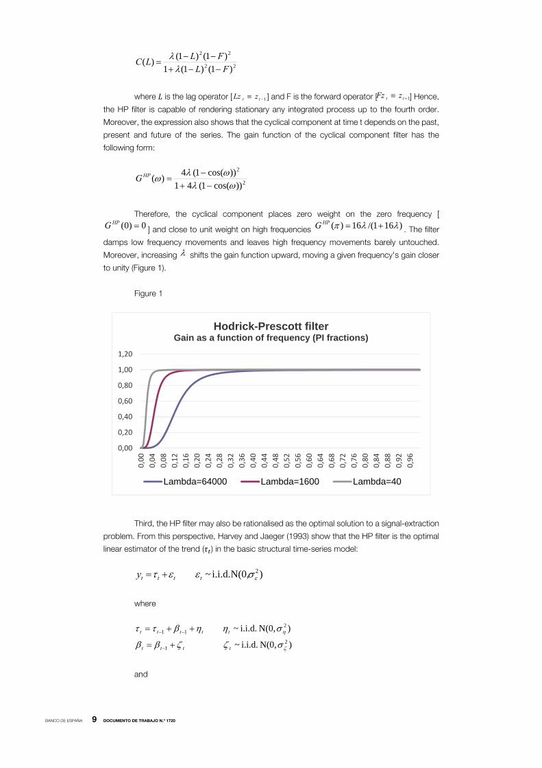
Therefore, the cyclical component places zero weight on the zero frequency [

0)0( HPG ] and close to unit weight on high frequencies )161/(16)( HPG . The filter

damps low frequency movements and leaves high frequency movements barely untouched.

Moreover, increasing shifts the gain function upward, moving a given frequency's gain closer

to unity (Figure 1).

Figure 1

Third, the HP filter may also be rationalised as the optimal solution to a signal-extraction

problem. From this perspective, Harvey and Jaeger (1993) show that the HP filter is the optimal

linear estimator of the trend ( ) in the basic structural time-series model:

)N(0, i.i.d. ~ 2 tttty

where

)N(0, i.i.d. ~

)N(0, i.i.d. ~2

1

211

tttt

ttttt

and

0,00

0,20

0,40

0,60

0,80

1,00

1,20

0,00

0,04

0,08

0,12

0,16

0,20

0,24

0,28

0,32

0,36

0,40

0,44

0,48

0,52

0,56

0,60

0,64

0,68

0,72

0,76

0,80

0,84

0,88

0,92

0,96

Hodrick-Prescott filter Gain as a function of frequency (PI fractions)

Lambda=64000 Lambda=1600 Lambda=40

1 tt zLz 1 tt zFz


2

2

Notice, however, that this rationalisation has the following assumptions: i) the series .

is integrated of order 2; ii) the cyclical component is a white noise process; and iii) that the chosen

value of the parameter corresponds to the ratio of the variance of the irregular component to

the variance of the innovation in the trend component.3

Fourth, the HP filter may be regarded as a member of the Butterworth family of filters

[Gómez (2001)]. Specifically, the gain of the two-sided Butterworth filter when based on the sine

function (BFS) is given by:

dBFSG 2

5. )2/(sin)2/(sin1

1)(

This filter depends on two parameters , the frequency for which the gain equals one

half and the integer number d, where larger values of d produce sharper filters. Notice that when

d equals 2 this is the gain of the HP filter. This expression also suggests that, in general, there is

a Butterworth filter that is more appropriate than the HP filter to estimate a cycle.

The HP filter has some drawbacks. First, has to be specified beforehand and

depending on the chosen rationalisation of the filter a different value of may be justified. In

fact, if one uses the minimisation approach the determination of may be seen as arbitrary. If a

signal extraction approach is used, then the value of should be estimated from sample data.

The interpretation of the HP filter as a high-pass filter suggests an objective way of determining

. The value of 1600 typically chosen for applications with quarterly data4 may be rationalised

as a high-pass filter that captures fluctuations with a period shorter than 8 years [Prescott (1986)].

The Butterworth filter interpretation gives some insight as to how to select . Indeed, the formula

. , where = 2 for the HP filter, gives us the relationship between and the

frequency for which the gain of the filter is 0.5. This would suggest using 6.6 with annual

data5 [Gómez (2001)].

The second drawback of the HP filter is that it induces spurious cycles in series with the

typical spectral shape. In fact, when applied to difference-stationary series point out that the HP

filter does not operate like a high pass filter [Cogley and Nason (1995)]. In this case, the filter is

equivalent to a two-step linear filter: difference the data to make them stationary and then smooth

the differenced data with an asymmetric moving average, so that the filter can generate business

cycle periodicity and comovement.

3. Trimbur (2006) develops a Bayesian generalisation of the Hodrick Prescott filter, in which a prior density is specified on .

This method ensures an appropriate degree of smoothness in the estimated trend while allowing for uncertainty.

4. With annual data, Hassler et al. (1994) and Baxter and King (1999) point out that results obtained with = 10 and annual

data are similar to those obtained with = 1600and quarterly data.

5. Ravn and Uhlig (2002) find that should be adjusted by multiplying it with the fourth power of the frequency ratio. That

would lead to 6.25 for annual data. Indeed, Maravall and del Rio (2007) show that this empirical rule turns out to be a first

order Taylor series approximation to the criterion of preserving the period corresponding to the frequency for which the filter

gain is .5.

ty

d25. )2/sin(2

5.

c


A third limitation is the poor behaviour of the HP filter for the most recent periods. To

minimise this problem, many users of the HP filter have traditionally used series extended with

the best available forecasts.6

On the advantages of the HP filter, it has been stressed that the method is simple and

that it provides a uniform framework that can be applied to different countries in a timely manner.

Since the method does not require subjective considerations, results can be easily reproduced.

2.1.2 FLUCTUATIONS WITHIN A RANGE OF PERIODICITIES

To some extent, the proliferation of techniques for measuring business cycles has resulted from

a lack of a widely agreed upon definition of the business cycle, an issue which Burns and Mitchell

(1946) viewed as central. In this sense, some proposals require the specification of the

characteristics of the cyclical component. The main aim of these approaches is to design a filter

which eliminates very slow moving (trend) components and very high frequency (irregular)

components, while retaining intermediate (business cycles) components. The desired filter is

what is known in the literature as an ideal band-pass filter, i.e. a filter which passes through

components of a time series belonging to a pre-specified band of frequencies (pass band), while

removing components at higher and lower frequencies.7 In formal terms, the ideal band-pass

filter ( ) has a gain function given by:

2

21

1

0

1

0

(

p

pp

p

BPI

|>| if

|| if

|<| if

=)G

which means that frequencies belonging to the interval pass through the

filter untouched, but all other frequencies are completely removed. defines the lower cut-

off frequency and the upper cut-off frequency. For empirical applications, there is then a

need to specify .The most widespread definition is to consider cycles between 6 and

32 quarters [Baxter and King (1999)].8

2.1.2.1 BAXTER AND KING (1999) FILTER [BK]

The aim of Baxter and King (1999) is to build the best linear band-pass filter that is constrained

to produce stationary outcomes when applied to growing time series.9 The ideal band-pass filter

requires an infinite-order moving average . However, in empirical applications series

are of finite length, so it is necessary to approximate the ideal filter with a finite symmetric moving

average

6. This practice is in line with Kaiser and Maravall (2001) results, which are confirmed by Mise et al. (2005). These authors

show through simulation exercises that applying the HP filter to a series extended with ARIMA forecasts and backcasts

generally provides a cycle estimator for recent periods that requires smaller revisions. This modification also improves the

detection of turning points.

7. Christiano and Fitzgerald (2003) propose a different approximation to the ideal band-pass filter.

8. For example, Englund et al. (1992) define the business cycle in terms of fluctuations longer than 18 quarters but shorter

than 32 quarters and Stock and Watson (1999) are interested in cyclical components of no less than 6 quarters in duration

but fewer than 24 quarters.

9. See Stock and Watson (2005) for an application.

BPIG

21, pp 1p

2p 21, pp

j

jbLb )(

jk

kjjk LaLa

)(


To find the weights, Baxter and King (1999) solve the following constrained minimisation

problem:

0)0(

|)()(|

.

}{2

k

kjd

ts

Min

where denotes the gain function of the ideal band-pass filter, the gain

function of the approximating filter and the gain of the approximating filter at frequency zero is

zero, so that the filter will render stationary (2) stochastic processes.

From the first order conditions, the optimal solution is given by:

kjba jj ,,1,0 where 12

k

bk

kjj

where

,,j

jπ

)(jω)(jω

jπ

ωω

bpp

pp

j

21sinsin

0

12

12

The weights of the optimal approximation are obtained in two stages. First, weights { }

corresponding to the ideal band-pass filter are computed, keeping the first + 1 ones. Second,

a correction factor is added, which depends on the extent to which truncation distorts the

desired behaviour at frequency zero. The cyclical component is obtained as:

tj

k

kjjt

BKt yLayC

)(

and its gain function is given by:

k

jj

BK jaaG1

0 )cos(2)(

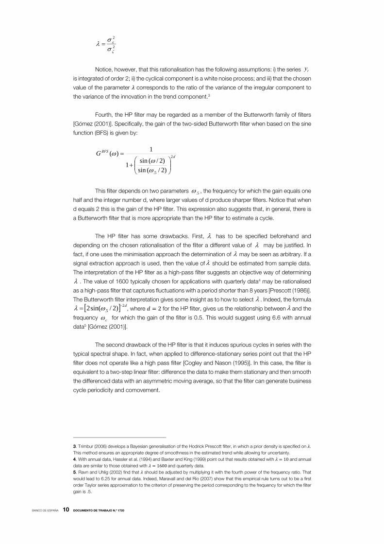
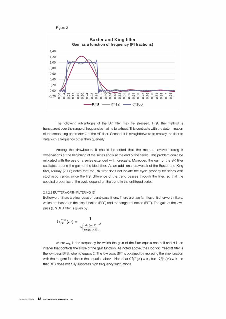
which is represented in Figure 2.

)( )( k

jb


Figure 2

The following advantages of the BK filter may be stressed. First, the method is

transparent over the range of frequencies it aims to extract. This contrasts with the determination

of the smoothing parameter of the HP filter. Second, it is straightforward to employ the filter to

data with a frequency other than quarterly.

Among the drawbacks, it should be noted that the method involves losing k

observations at the beginning of the series and k at the end of the series. This problem could be

mitigated with the use of a series extended with forecasts. Moreover, the gain of the BK filter

oscillates around the gain of the ideal filter. As an additional drawback of the Baxter and King

filter, Murray (2003) notes that the BK filter does not isolate the cycle properly for series with

stochastic trends, since the first difference of the trend passes through the filter, so that the

spectral properties of the cycle depend on the trend in the unfiltered series.

2.1.2.2 BUTTERWORTH FILTERING [B]

Butterworth filters are low-pass or band-pass filters. There are two families of Butterworth filters,

which are based on the sine function (BFS) and the tangent function (BFT). The gain of the low-

pass (LP) BFS filter is given by:

dBFSLPG

)2/(sin

)2/(sin15.

1)(

where . is the frequency for which the gain of the filter equals one half and d is an

integer that controls the slope of the gain function. As noted above, the Hodrick Prescott filter is

the low pass BFS, when d equals 2. The low pass BFT is obtained by replacing the sine function

with the tangent function in the equation above. Note that , but ,so

that BFS does not fully suppress high frequency fluctuations.

-0,20

0,00

0,20

0,40

0,60

0,80

1,00

1,20

1,40

0,00

0,04

0,08

0,12

0,16

0,20

0,24

0,28

0,32

0,36

0,40

0,44

0,48

0,52

0,56

0,60

0,64

0,68

0,72

0,76

0,80

0,84

0,88

0,92

0,96

Baxter and King filter Gain as a function of frequency (PI fractions)

K=8 K=12 K=100

0)( BFTLPG 0)( BFS

LPG


BFS and BFT can be obtained as optimal (minimum mean squared) estimators of the

signal in the signal ( ) plus noise ( ) model [Gómez (2001)]:

ttt nsy

where and and are zero mean constant variance independent

processes. In the case of BFS , so that is IMA(d,0) process, and in the case of BFT

. , so that is a n IMA(d,d) process.

Butterworth band-pass filters BPF (L, F) in the time domain can be expressed as:

dddd

dd

FFLLFL

FLFLBPF

)1()1()1()1()1()1(),( 2222

22

where , and and .

are the lower and upper limits of the band-pass, respectively. Note that larger values of d produce

sharper filters.

These Butterworth band-pass filters also admit a model-based interpretation.10

Specifically, Gómez (2001) shows that the band-pass BFT can be obtained11 as the best linear

estimator, in the mean squared sense, of the signal in the signal-plus-noise model:

ttt sy

where follows the model and and are

white noise processes. Note that the autoregressive model for the signal has two complex roots

of unit modulus.

Figure 3

10. Valle e Azevado et al. (2006) propose a multivariate generalization of a band-pass filter.

11. Harvey and Trimbur (2003) give a model-based interpretation for band pass BFS filters.

-0,20

0,00

0,20

0,40

0,60

0,80

1,00

1,20

1,40

0,00

0,04

0,07

0,11

0,14

0,18

0,21

0,25

0,28

0,32

0,35

0,39

0,42

0,46

0,49

0,53

0,56

0,60

0,63

0,67

0,70

0,74

0,77

0,81

0,84

0,88

0,91

0,95

0,98

Butterworth and Baxter and King band pass filters

Gain as a function of frequency (PI fractions)

Baxter and King Butterworth Ideal

tstd aLs )(

1)( Lsd

s LL )1()(

2cos2cos 1212 pppp 22a 1p 2p

td

td LsLL )1()cos21( 22 t t


The use of Butterworth band-pass filters has two main advantages with respect to the

usual finite moving average filters, such as Baxter and King (1999). First, because rational

functions are used instead of polynomials in the lag operator, a better approximation to an ideal

gain function is possible (Figure 3). Second, the number of forecasts and backcasts required for

the finite sample implementation of Butterworth filters is much smaller than for finite moving

average filters.

2.1.3 WAVELET-BASED METHODS [W]

Donoho (1993) introduced a method called wavelet denoising or wavelet shrinkage that has been

applied by e.g. Aguiar-Conraria and Soares (2011) and Tiwari et al. (2014) to obtain measures of

the output gap. This method may be thought of as a generalisation of Fourier analysis. Traditional

Fourier analysis does not account for variation through time of the frequency components of a

series. In contrast, wavelet analysis is able to assess through the relative importance of cycles of

different duration, so it is more suitable to study irregular series.

The idea of this method is analogous to a series of low pass filters: large wavelets

encode the general trend in output, whereas small wavelets characterise the details. Therefore,

by filtering out the coefficients of the small wavelets it is possible to obtain the dominant features

of a series by applying the inverse wavelet transform. To be more specific, the trend component

of the output series is obtained through the following three steps.

First, the output series is first expressed as the orthogonal wavelet series:

)()(1

0

12

0tdtdy jk

n

jjk

kot

j

and the coefficients of the wavelet representation ( and ) are obtained. In this

expression, is a father wavelet, also referred to as a scaling function that represents the

smooth baseline of the series where, given a mother wavelet , an orthonormal .

basis is defined as:

)2(2)( 2/ ktt jjjk

where the parameters j and k dilate and translate the function.

Second, the wavelet coefficients are shrunk applying a thresholding non-linear

transformation:

jk

jkjkjk dif

difdd

0ˆ

to eliminate the wavelet coefficients that are thought to correspond to business cycle

frequencies.

od jkd)(t

)(t )}({ tjk


Third, the inverse wavelet transform is applied in order to obtain the measure of trend

output:

)(ˆ)(ˆ)(1

0

12

0tdtdyT jk

n

jjk

kot

W

j

This filter has more degrees of freedom than a band-pass filter. It is not limited to a

particular choice of wavelets, while the band-pass filter is defined exclusively in the space formed

by sines and cosines. This could make the method more appealing since, at least theoretically,

it would cope better with a changing economic structure. Second, the features of the filter can

be modified according to the number of wavelet coefficients removed and the shrinkage

threshold. Among its drawbacks, there exists a wide choice of wavelets and the methodology to

select the most appropriate one depends on subjective considerations.

2.2 Model-based approaches

2.2.1 LINEAR DETRENDING [LD]

One simple method is to assume the trend is a linear function of time.12 The cyclical component

emerges in this method as a residual from the trend line. Specifically,

tyT tLD

t )(

where denotes the logarithm of output and denotes time.

The main virtue of this procedure lies in its simplicity. However, one undesirable

implication is that the long-run evolution of a time series is a function of time. The idea that

economic time series are better characterised by stochastic trends led to the development of a

set of techniques aimed at taking into account this feature.

2.2.2 A FORECASTING PERSPECTIVE. BEVERIDGE AND NELSON (1981) [BN]

The Beveridge and Nelson (1981) procedure decomposes a non-stationary time series as the

sum of a permanent and a transitory component. The trend component is defined in terms of

the long-run forecast of output and the corresponding cyclical component has the interpretation

as the negative of output growth in the excess of the normal growth that would be forecast given

the current state of the economy.

The starting point of this approach is that many economic time series are well

represented by an ARIMA process for which the first differences are a stationary process of

autoregressive-moving average form. If we denote by the first difference of the logarithm of

output, then:

ttp

qt Ld

L

Ldy

)()()(

12. In empirical investigations segmented trends are often used [e.g. Drake and Mills (2010)]. This implies that trend growth

is not constant over time, although it is constant inside particular time intervals. Segmented trends allow for the incidence of

supply shocks, which may permanently alter both the level and trend growth rate of potential output.

ty


where is the mean of the process, ~ i.i.d. N (0, ) and and are

polynomials in the lag operator of orders p and q, respectively, with roots outside the unit circle.

The following additive decomposition of into a stationary and a non-stationary

component:

ttt Ldy )(~)1(

where .

The sum of the first two terms on the right hand side represents the first difference of

the trend component, which follows a random walk with drift, while the third term represents the

first difference of the cyclical component.

ttBN

t dyT )1()(

ttBNt LyC )(~)(

Beveridge and Nelson (BN) define the trend as the value the series would have if it were

on its long-run time path in the current time period. This definition of trend is then the long-run

forecast of the series adjusted for its mean rate of change. This trend may be expressed as a

weighted average of the current and past values of the series :

tq

p

p

qt

BNt y

L

LyT

)()(

)1()1(

)(

This expression shows that future information will not modify the trend component and

that the weights used to calculate the trend will differ depending on the stochastic properties of

the series.13

Three drawbacks of the BN decomposition should be noted [Beveridge and Nelson

(1981) and Canova (1998)]. First, since trend and cycle are driven by the same shock, the

innovations to these components are perfectly correlated. This may not correspond to the

conventional view about the behaviour of these components. Second, the trend component may

be too "noisy", since the variance of the innovation in the permanent component may be larger

than the innovation of the observed data.14 Third, it may be the case that different ARIMA models

fit the data fairly well. However, because ARIMA models with similar short-run properties may

have very different long-run properties, alternative specifications may lead to very different

decompositions into trend and cycle.

13. Proietti and Harvey (2000) propose a Beveridge-Nelson smoother, which is two-sided signal extraction filter for trends.

This estimator is the optimal (minimum mean square error) estimator of the trend when the ARIMA model can be

decomposed into an uncorrelated random walk and stationary cycle components.

14. Morley et al. (2003) show that the BN decomposition is identical to that obtained with a structural time series model,

once the restriction of uncorrelatedness between innovations in the trend and cyclical components is allowed for. Morley

(2011) points out that these two models have very different implications in terms of the uncertainty about the measure of the

permanent component.

t2 )(Lq )(Lp

ty

)1()()(~ LL

ty


2.2.3 A STRUCTURAL TIME SERIES APPROACH [STS]

Univariate structural time series models are models that are set up in terms of unobserved

components, which have a direct interpretation [see e. g. Harvey (1985)]. The whole model is

handled within a unified statistical framework that produces optimal estimates with well-defined

properties. A traditional formulation is the trend plus cycle plus irregular model

tttty

where is the logarithm of output, is a trend, is a cycle, and is an irregular

component and all components are assumed to be uncorrelated with each other. Since a

deterministic time trend seems too restrictive, in this type of models a more flexible approach is

used by letting the level and slope parameters change over time. Specifically, these parameters

are typically assumed to follow random walks.15

tttt 11

ttt 1

where and are white noise processes with variances and .

The stochastic cycle is generated as:

t cos t1 sin t1 t

tttt sin 11 cos

where is a damping factor such that 0 ≤ < 1, is the frequency of the cycle

expressed in radians and and ∗ are white noise processes with variances and ∗, respectively. In general, the cyclical component is a stationary variable.16 Finally, the irregular

component is also a white noise process with variance .

Once the model is specified, it can be estimated by casting it in space-state form. The

Kalman filter may then be used and the Kalman smoother allows the extraction of trend and

cycles:

ttSTS

t yT ̂)( ; tt

STSt yC ̂)(

One drawback of this approach is that it assumes that output is integrated of order

two.17 Most macroeconomists, however, consider that output growth is stationary. In practice,

the standard STS often results in the irregular component disappearing, so that the cycle is quite

noisy [Harvey et al. (2007)]. The reduced-form of this structural model is a restricted ARIMA

(2,2,4) model with some nonlinear restrictions on the coefficients. To the extent that the series

under study departs from this ARIMA model, results with the STS model may be unreliable.

15. Note that the level and slope are allowed to evolve over time and that the deterministic trend is a limiting case in which

these variances are zero.

16. This is the case provided that 0 ≤ < 1. In this case, the cyclical component follows an ARMA (2,1) process.

17. This is a particular feature of the basic structural model.

t t t

t t 2

2

2

ty


The STS is generalised in Harvey and Trimbur (2003). These authors propose a model

with a stochastic trend of order m (instead of the standard order 1) and a stochastic cycle of

order n (instead of the standard order 1). They find that the generalised cyclical component

provides a smoother, more clearly defined cycle.18

2.2.4 MARKOV SWITCHING MODELS [MS]

The Markov switching model, due to Hamilton (1989), divides the business cycle into two phases,

negative trend growth and positive trend growth, with the economy switching back and forth

according to a first order Markov process. Hamilton proposes modelling output as the sum of

two independent unobserved components, one following a random walk with drift, which evolves

according to a two-state Markov process, and the other following an autoregressive process

with a unit root. Specifically, the output series is decomposed as

ttty

where the first component is assumed to follow a random walk with drift, which evolves

according to a two-state Markov process

ttt S101

1,0tS

pSSob tt )11(Pr 1 pSSob tt 1)10(Pr 1

qSSob tt )01(Pr 1 qSSob tt 1)00(Pr 1

and the second component follows an ARIMA (p,1,0) process. In this model, need

not change every period, in contrast with a STS model, even though follows an AR(1)

process. The reason is that the innovation follows a discrete distribution instead of a Gaussian

one.

The attractiveness of this specification comes from the fact that it allows for non-linear

dynamics such as asymmetry. For estimation purposes a non-linear iterative filter is employed to

obtain maximum likelihood estimates of population parameters.

An alternative possibility to deal with asymmetric behaviour is to employ the model by

Kim and Nelson (1999). They propose modelling output as two independent unobserved

components,19 one a stochastic trend with time-varying level and slope parameters, and the

other following a mixture of symmetric and asymmetric shocks. Specifically, the output series is

decomposed as:

ttty

18. This generalised model is studied from a Bayesian perspective in Harvey et al. (2007). This perspective allows flexible

restrictions to be placed on key parameters, such as the period in the stochastic cycle and avoids fitting implausible models.

19. Sinclair (2010) develops an unobserved components model that allows for both asymmetric transitory movements and

correlation between the permanent and transitory innovations.

tt


The stochastic trend follows a conventional specification:

tttt 11

and to allow for regime shifts or asymmetric deviations transitory shocks have the

following specification:

tttt SL )(

1,0tS

pSSob tt )11(Pr 1 pSSob tt 1)10(Pr 1

qSSob tt )01(Pr 1 qSSob tt 1)00(Pr 1

. is an asymmetric, discrete shock (the size of the pluck) which is dependent on an

unobserved Markov-switching state variable whose transition probabilities are specified above

and which accounts for the persistence of normal or recession periods and is a symmetric

shock. During normal times, and the economy is near the potential or trend output. During

recession times, , the economy is hit by a large negative shock and firms use factors

suboptimally and output is below its production frontier.

According to Friedman (1964, 1993), recessions are periods where output is hit by large

negative transitory shocks, labelled plucks. Following the trough, output enters a high growth

recovery phase, returning to the trend. Output then begins a normal, slower growth, expansion

phase. Thus, Friedman’s view is that recessions are entirely transitory deviations from trend, not

movements in the trend itself. In this regard, Kim et al. (2005) have proposed a model with a

post-recession bounce-back effect in the level of output. Their model is described as:

t

h

jjttt SSL

110)(

where is a latent first–order Markov switching process, which equals 1 in recessions.

When = 0 the model collapses to Hamilton (1989), whereas if is positive, the summation

term implies that GDP will be above average for some time after a recessionary regime, indicating

the existence of a post-recession bounce back effect. This implies that a recessionary shock is

less persistent than an expansionary one.

t

tS

t0tS

1tS


3 Multivariate approaches

By their own nature, it is hard or even impossible to give univariate approaches a structural

interpretation. Against this background, it seems natural to expand the information set used in

the estimation of the output gap and employ multivariate approaches that can be given an

economic interpretation. To this end, a variety of methods have been proposed in the literature,

the most widespread of which are examined below.

3.1 Okun’s law [OL]

In the short-run, when aggregate demand fluctuates and firms respond by adapting their output,

they mostly resort to changes in their labour input. This results in a negative empirical relationship

between fluctuations of output around its trend and fluctuations of unemployment

around its trend , which is known as Okun’s law.

)()( tttt uCyC

Although there are a number of reasons for which Okun’s law is not expected to hold

exactly, even in the short-run, such as productivity shocks, this empirical relationship generally

provides a satisfactory approximation and, since Evans (1989), has been exploited by many

authors to assess the cyclical position of the economy [e.g. Apel and Jansson (1999), Doménech

and Gómez (2006)].

Evans (1989) uses a bivariate structural VAR to describe (the log difference of) output

and unemployment dynamics. The identifying restriction is that output shocks

contemporaneously cause the unemployment rate. This means that the negative correlation

between and is attributed to an Okun’s law equation, in which is weakly exogenous

and the unemployment equation is interpreted as a dynamic version of Okun’s law. The

corresponding structural model is:

tyttt euLyLy ,11 )()(

tutttt euLyLyLu ,11 )()()(

where are orthogonal structural shocks.

Based on this model, Evans (1989) develops a cyclical measure based on Okun’s law.

Okun defined potential output as the level of output that would yield an unemployment rate equal

the conditional mean of the unemployment rate. To obtain the cyclical measure, it is assumed

that the sequence of future output growth rates is such that unemployment remains at its

unconditional mean level and that the unemployment equation is invariant to these changes. If

we denote as the level of output conditional of unemployment being at its unconditional

mean, then a definition of the output gap, à la Beveridge and Nelson, is given by:

OLttt

OLt yyEyC )()(

)( tt yC)( tt uC

ty tu ty

tuty ee ,, ,

OLty


Here, the extra growth available is measured along an unconditional mean

unemployment rate, rather than along the path corresponding to the normal dynamic response

of the economy.

Among the drawbacks of the Okun’s law, it has been pointed out that the

unemployment rate is just a proxy variable for all the ways in which output -which depends on

labour, capital and technology-, is affected by idle resources. Furthermore, the unemployment

rate is but one factor in determining the total amount of labor used as an input; other factors

include the fraction of the population that is in the labor force and the number of hours that

employed workers are used. Finally, Blanchard and Quah (1989) argue that Okun’s law

coefficient is mongrel since the relationship between output and unemployment depends on

whether shocks are demand or supply side.

3.2 A production function approach [PF]

The traditional production function approach is intended to provide a comprehensive and

consistent economic framework for measuring potential output and the output gap. The method

explicitly models output in terms of underlying factor inputs, and not just labour, as in an Okun’s

law approach, and involves specifying and estimating production functions that link output to

capital, labour and total factor productivity. Potential output is then calculated as the level of

output that results when the rates of capacity utilisation are normal, when labour input is

consistent with the natural rate of unemployment, and when total factor productivity is at its trend

level. This method is currently being used by central banks and international organizations.

The method first requires choosing an appropriate specification for the production

function. This allows for an explicit accounting for growth in terms of the contributions of factor

inputs and a residual driven by total factor productivity. In what follows we describe, for illustrative

purposes, the production function method as used by the European Commission [Havik et al.

(2014)]. Potential output is computed on the basis of a two-factor Cobb-Douglas production

function with constant returns to scale. Using this production function, the measure of potential

output is obtained by combining a measure of trend productivity with the actual capital stock

and estimates of potential employment. The chosen measure of potential employment is defined

as the level of labour resources that might be employed without resulting in additional inflation.

More specifically, the production function is assumed to be of the Cobb-Douglas form:

tttt lky )1(

where denotes the logarithm of total factor productivity, the logarithm of capital,

. the logarithm of labour input and is the elasticity of labour with respect to output, which

can be estimated from the wage share under the assumption of constant returns and perfect

competition. Potential output is obtained from:

)()1()()( tNAWRU

tttKF

ttPF

t lTkTyT

where is a measure of the logarithm of trend factor productivity obtained with

a bivariate Kalman Filter which exploits the link between the TFP cycle and the degree of capacity

utilisation and is a measure of trend employment defined as the level of labour input

that might be employed without additional inflation.

It has been stressed that the PF approach has a number of advantages. For instance,

it can provide a broad and coherent assessment of the economic outlook. Furthermore, it allows

t tk

tl

)( tKF

tT

)( tNAWRU

t lT


)0(S

for an explicit accounting for growth in terms of contributions of capital, labour and total factor

productivity. Besides, it is possible to estimate the impact of current or projected developments

on future levels of potential output, although this requires being able to project potential labour

and trend TFP.

There are, however, a number of drawbacks. Some assumptions on the structure of the

economy need to be made and they may not fully correspond to reality. For instance, the

assumption of perfect competition does not seem to hold in real world economies. Moreover,

the production function may not exhibit constant returns to scale and the Cobb-Douglas

functional form may not be entirely satisfactory. For instance, Dimitz (2001) uses a Constant

Elasticity of Substitution (CES) production function, which is more general that the Cobb-

Douglas, and allows the substitution elasticity among factors to differ from one. Furthermore,

estimating the output gap with a PF approach entails using measures of the trend of the inputs,

which are not straightforward to obtain.20 Moreover, as noted by Fernald (2014), production-

function measures of potential output are inherently cyclical because investment is cyclical.

Finally, the standard production function approach is a one sector model, but Basu and Fernald

(2009) show that two-sector models -where one sector produces consumption goods and the

other produces investment goods- fit the data much better, since they are able to capture the

rapid technological change in the production of equipment goods.

3.3 Aggregate supply and demand shocks. Blanchard and Quah (1989) [BQ]

Blanchard and Quah (1989) interpret fluctuations in GDP and unemployment as due to two types

of disturbances: disturbances with a permanent effect on output, mostly supply shocks, and

disturbances that only have a transitory effect on output, mostly demand shocks. This

interpretation of disturbances with permanent effects as supply shocks and disturbances with

transitory effect as demand shocks is motivated by a traditional Keynesian view of fluctuations.

BQ employ a simple model based on Fisher’s nominal wage contracting theory. In their model,

due to nominal rigidities, demand disturbances have short-run effects on output and

unemployment, but these effects disappear over time. In the long-run, only supply shocks affect

output. Neither of the disturbances have a long run impact on unemployment.

To identify structural disturbances they introduce a Structural Vector Autoregression

(SVAR) with long-run identifying restrictions. This approach assumes that the vector of variables

of interest has the following structural interpretation, which is based on economic theory:

. where is a 1 vector of deterministic components, is a 1 vector of

structural shocks with and . The assumption that the variance-covariance

matrix is the identity is simply a convenient normalisation. ( ) shows the transmission

mechanism through which structural disturbances affect the economy. Formally, it is a matrix

polynomial in the lag operator L. . Blanchard and Quah (1989) introduce long-

run identification restrictions. Heuristically, identification is achieved if the number of restrictions

equals the number of unknowns in .

In their empirical application, BQ use a bivariate model and one of the series has a unit

root. In that framework, independence of structural shocks imposes three restrictions on the four

elements of (0). To identify their model, BQ additionally impose that demand disturbances only

have a transitory effect on output .

20. Staiger et al. (1997) show that NAIRU estimates are fairly uncertain and great care is needed when using this measure

in policy-making.

tt LSdx )( t0tE nt IE

t'

0

)(j

jj LSLS

0)1(12 S


Following estimation, a decomposition of output in terms of the structural disturbances

is given by:

tt

ty

pt

pyyt LSLSdy )()(

where is the vector of structural shocks with a permanent effect on output and .

is the vector of structural shocks with a transitory effect on output. The first difference of trend

output is the sum of the first two terms of the right hand side. Thus, trend output corresponds

to the permanent component of output. One advantage of this method is that trend or potential

output is not restricted to be a simple random walk and will generally display richer dynamics.21

Some authors have criticised the BQ decomposition because it does not correctly

identify supply and demand shocks, given that some supply disturbances have transitory effects

on output and some disturbances may have a permanent effect on output. Furthermore, some

care is needed to correctly interpret SVAR results. Indeed, Faust and Leeper (1997) point out

some reasons why structural inferences under long-run identification restrictions may be

unreliable. For instance, in finite samples, the long-run effect of shocks may be imprecisely

estimated. Moreover, Fernald (2007) has shown that VARs identified with long-run restrictions

are quite sensitive to controlling for breaks in labor productivity.

3.4 Phillips curve models [PC]

Potential output is a key element in price setting models built on the Phillips curve. According to

this view, an excess of output over potential implies tight labour and product markets, so that

inflation will tend to rise in the short-run, provided that inflation expectations and supply

conditions remain unchanged. Conversely, when the output gap is negative and labour and

product markets are slack, inflation will tend to fall in the short-run. In the short-run, the Phillips

curve shows a positive relationship between the change in the price level and deviations of output

relative to potential for a given expected inflation rate.

The idea of these estimation procedures is that the joint estimation of the Phillips curve

and the output gap should provide more information that the univariate estimation of the output

gap. The output gap is then determined as the one most consistent with observed inflation

subject to the smoothness restrictions implicit in the stochastic trend specification of GDP. The

fact that potential output and the output gap are not observable suggests the use of multivariate

unobserved components models linking these concepts to observed variables. In order to

identify the unobserved components, the framework requires that the stochastic process of

potential output be specified and some restrictions on the correlation between innovations to

unobserved variables and the innovation of the economic equation. A model is cast in state-

space form and then a Kalman smoother is used to estimate its parameters and to derive the

unobserved output gap series.

3.4.1 TRADITIONAL PHILLIPS CURVES [TPC]

Kuttner (1994) first suggests the use of a multivariate unobserved components model to estimate

potential output. Specifically, this author uses a Phillips curve in which the current change of

inflation is related to the lagged output gap and a vector of additional variables to capture the

effects of temporary relative price shocks on inflation. The essence of traditional Phillips curve

models of price adjustment is that the level of output relative to potential ( ) is systematically

21. The BQ definition includes in the trend the dynamics of permanent structural shocks, thus allowing for the gradual

absorption of technology shocks by the economy.

pt

tt

tz

TPCtC


related to inflation and a set of exogenous variables , such as nominal oil prices or the

exchange rate.

tttTPCtt zyC 110 )(

This accelerationist specification is consistent with a Phillips curve model in which

expected inflation equals lagged inflation, is the slope of the Phillips curve and represents

the elasticities of inflation with respect to exogenous variables.

To identify the model, Kuttner (1994) assumes that the output gap is an AR(2) process

and potential output follows a random walk with drift. The output and inflation equations together

form a bivariate unobserved components model that may be estimated by maximum likelihood

through the use of the Kalman filter.

The method includes a fair amount of structural information while maintaining

parsimony. The main advantages it offers is that it may be readily updated as fresh inflation and

output data are released and no independent measure of the NAIRU is needed, nor does it

require any subjective judgement. Additionally, it offers a measure of the time-varying uncertainty

associated with the potential output series.

3.4.2 NEW KEYNESIAN PHILLIPS CURVES [NKPC]

In traditional formulations of the Phillips curve, inflation expectations are fully backward looking,

so that expected inflation simply depends on lagged inflation. In contrast, in modern New

Keynesian Phillips Curve models [NKPC], forward looking profit maximising firms set prices on

the basis of expected marginal cost, so that current inflation depends on expected future inflation

and the output gap. In practice, hybrid models, in which current inflation depends both on lagged

and expected future inflation seem to provide a better description of the inflationary process.

Doménech and Gómez (2006) estimate a multivariate model including a NKPC.

Expected inflation is generated endogenously within the model:

tttNKPCttttt zyCE 11011 )()1()(

The model includes equations for the Phillips Curve, Okun’s Law, and investment

equation and the assumption that the output gap is an AR(2) process and potential output follows

a random walk with drift. The model is estimated by maximum likelihood using a Kalman filter.

3.5 Natural rate of interest [NRI]

Laubach and Williams (2003, 2015) consider a multivariate model that jointly estimates the natural

rate and the output gap, taking into account the comovements in inflation, output, and interest

rates. The natural rate of interest changes over time owing to shifts in aggregate supply and

demand. Specifically, the natural rate of interest, denoted r∗ is given by:

∗ = ∆ ( ) +

where ∆ ( ) is the estimated trend growth rate of potential GDP that is assumed

to be a random walk process, z is an unobserved component that is also assumed to follow a

random walk process, and c is an estimated coefficient that measures the influence of the trend

growth rate on the natural rate of interest. The model is estimated using the Kalman filter and

t tz

0 1


also uses an IS curve relating the output gap to its own lags and the lagged “real rate gap” –the

difference between the actual real interest rate and the natural rate. The output gap is informed

by a Phillips curve that relates core inflation to its own lags, the lagged output gap, and

movements in the relative prices of oil and non-energy imports.

3.6 Real Business Cycle models [RBC]

Real business cycle (RBC) models are dynamic, stochastic general equilibrium models of the

economy that generate empirical predictions for a wide array of macroeconomic variables. RBC

models view aggregate economic variables as the outcomes of the rational decisions made by

many individual agents acting to maximise their utility or profits subject to production possibilities

and resource constraints. Moreover, the general equilibrium of the model is always fully specified.

A stylised RBC model is made by an economy populated by many identical agents that

live forever. Each individual has to maximise his lifetime utility subject to the production

technology and a sequence of resource constraints. Given the specific functional forms for the

utility function and the production function and some initial conditions, it is possible to derive the

optimal decisions of the individual for his consumption, work and investment decisions. This

model (see King, Plosser and Rebelo (1988) for details) then predicts that all quantity variables

(with the exception of work effort) grow at the same rate, which is given by the growth rate of

technological progress. Therefore, the logarithms of the balanced-growth great ratios isolate two

linearly independent cointegrating vectors.22

The starting point is the structural model where is a nx1 vector of

structural shocks with and a block diagonal variance covariance matrix , which is

partitioned conformably with , where is a 1 vector of structural shocks

with permanent effects, is a ( − ) 1 vector of structural disturbances with transitory effects.

Permanent shocks are assumed to be orthogonal but transitory shocks may be correlated.

Furthermore, the cointegration restrictions derived from the theoretical model impose constraints

on the matrix of long-run multipliers , which allow us to identify the permanent components.

Following estimation of the structural model, King et al. (1991) suggest employing a

multivariate version of the BN decomposition.

tt

tpt

ppt

pt LSLSSdx

)()()1( 11111

where

j

j

pj

p LSLS

0

11 )(

and

1

11jm

mpj SS

Its interpretation in terms of a trend-cycle decomposition is as follows. The sum of the

first two terms on the right hand side represents (the first difference of) the trend, while the sum

of the third and fourth represents (the first difference of) the cyclical component. Note that the

trend is a random walk with drift, a feature that has been criticised above. This contrasts with

BQ’s approach, which includes the diffusion process associated with permanent shocks in trend

output.

22. King et al. (1991) point out that some conclusions obtained with a basic one-sector model are also valid in richer models.

tt LSdx

)( t

0tE

)'','( t

tp

tt pt

tt

)1(S


It should be emphasised that although the economic theory which motivates the

identifying restrictions is different in BQ’s and King et al. (1991)’s approaches, the econometric

methodology is, broadly speaking, the same.23

3.7 Dynamic Stochastic General Equilibrium models [DSGE]

In recent years, Dynamic Stochastic General Equilibrium (DSGE) models have become widely

used to project the economy and to derive policy implications. This class of models combine

Keynesian and Real Business Cycle features in the sense that wages and prices are sticky and

classical theory explains the long-run. This class of models typically incorporates various other

features such as habit formation, costs of adjustment in capital accumulation and variable

capacity utilization. They are generally estimated with Bayesian techniques using a limited

number of variables [see e.g. Smets and Wouters (2003), Edge et al. (2008) or Fueki et al. (2016)].

DSGE models allow us to consider three different notions of potential output [Vetlov et

al. (2011)]. First, the trend level of output is equal to the sequence of permanent stochastic

technology shocks that characterize the balanced-growth part of the model. Second, the efficient

level of output is the level of GDP that would prevail if goods and labour markets were perfectly

competitive. Third, the natural level of output is the level of output under flexible wages and prices

and imperfectly competitive markets. Estimates of trend level of output using DSGE models focus

on the long-run and are typically close to those obtained from conventional approaches. In

contrast, efficient and natural levels have a business cycle dimension related to the shocks that

push the economy temporarily away from the steady state, so are generally more volatile. Their

use depends on the aim of the analysis. From the point of view of inflation, interest should focus

on the natural output gap, since under certain assumptions this measure of the output gap is a

key driver of inflation. From the point of view of welfare, policymakers should aim at stabilising

the efficient output gap.24

Among the advantages of DSGE models, they allow for a deeper structural

interpretation. The joint estimation of potential output and structural shocks within the general

equilibrium framework allows conducting a quantitative and internally consistent assessment of

inflation pressures and a normative evaluation of alternative monetary measures. Among the

drawbacks, it has been pointed out that the flexible-price and natural rate gaps are highly

dependent on modelling assumptions [Kiley (2013)].

23. This is best seen by rewriting the model of King et al. (1991) in terms of stationary variables. The productivity shock has

a long-run effect on output, but no long-run effect on the consumption and investment ratios.

24. Unless the so-called “divine coincidence” holds, stabilizing the efficient output gap is not the same as stabilising the

natural output gap.


4 Conclusions

In this paper, we examine different approaches used in the literature to estimate potential or trend

output and the output gap, highlighting their advantages and drawbacks. Potential output and

the output gap are unobservable and an objective definition of the business cycle does not exist.

Both reasons have led to a proliferation of techniques for measuring business cycles. However,

different techniques employ, explicitly or implicitly, different hypotheses, of either statistical or

theoretical nature. Comparisons of techniques should take this fact into account. Tables 1 and

2 summarize some of the main characteristics of the univariate and multivariate methods

presented in this paper.

Table 1

Univariate estimation methods

Model based Decision

variables Complexity

Need or

advisability of

using forecast

Hodrick & Prescott No Smoothness

parameter Low Yes

Baxter & King No Pass band

Filter length Low Yes

Butterworth filtering No Pass band

Filter length High Yes

Wavelet-based

methods No Wavelet basis High Yes

Linear detrending Yes None Low No

Beveridge & Nelson Yes ARIMA model High Yes

Structural time series Yes STS model High No

Hamilton Yes Regime switching

model High No

Kim & Nelson Yes Regime switching

model High No

It is convenient to classify existing approaches to estimate the output gap into different

groups, according to the criteria used. Univariate methods are based on statistical assumptions,

which define what is considered to be the output gap or trend output. These procedures could

be summarised as follows: on the positive side, they are generally simple procedures that do not

require judgmental assumptions about the structure of the economy. As a consequence, they

can be applied to a large number of countries in a homogeneous and timely way. Nevertheless,

the main disadvantage of these methods is the lack of economic theory criteria underlying their

application, and the fact that they do not incorporate potentially useful information on some other

variables into the analysis.


On the contrary, the use of multivariate methods within the context of a model based

on economic theory is attractive. Multivariate approaches exploit economic theory to estimate

potential or trend output, a feature that is certainly attractive. However, it has to be acknowledged

that views on the structure of the economy are likely to differ widely across researchers.

Moreover, cross-country comparisons have to be made with due care due to differences in the

economic structure of different countries.

Table 2

Multivariate estimation methods

Underlying

economic theory Decision variables Complexity

Okun's law Okun's law VAR model Medium

Production function Production function Production function

Cyclically adjusted inputs High

Blanchard & Quah Supply and demand

shocks SVAR model High

Phillips curve Phillis curve Output gap time series

process High

Natural rate

of interest

Natural rate

of interest

Lags in the Phillips curve,

Output gap time series

process

High

RBC model General equilibrium VECM model High

DSGE model General equilibrium Model specification High

Our main conclusion is that the different methods that have been proposed in the

literature have their particular advantages and disadvantages and none of them takes priority

over the rest. Therefore, it seems adequate to examine several of them in order to obtain a more

reliable description of the state of the cyclical position of the economy. However, nowadays the

most widespread technique in policy institutions is the production function approach and DSGE

methods are increasingly being used. While time-specific circumstances may make it advisable

to focus on a particular measure, it is nonetheless true that diagnosis of the cyclical position

gains in solidity insofar as different measures convey the same message. This is especially

important if these measures play some role in economic policy decision-making.


REFERENCES

AGUIAR-CONRARIA, L. and M.J. SOARES (2011). “Business cycle synchronization and the Euro: a wavelet analysis,”

Journal of Macroeconomics, 33(3):477-489.

APEL, M. and P. JANSSON (1999). “A theory consistent system approach for estimating potential output and the NAIRU,”

Economics Letters. 64:271-275.

BAXTER, M. and R. G. KING (1999). “Measuring Business Cycles. Approximate Band-Pass Filters for Economic Time

Series,” The Review of Economics and Statistics, 81(4):575-593.

BASU, S. and J. FERNALD (2009). “What Do We Know and Not Know About Potential Output?,” Federal Reserve Bank of

St . Louis Review. July/August:187-213.

BEVERIDGE, S. and NELSON, C.R. (1981). “A new approach to decomposition of economic time series into permanent

and transitory components with particular attention to measurement of the 'business cycle',” Journal of Monetary

Economics, 7:151-174.

BLANCHARD, O. J. and D. QUAH (1989). “The Dynamic Effect of Aggregate Demand and Supply Disturbances,” The

American Economic Review, 79(4):655-673.

BURNS, A.M. and W. C. MITCHELL (1946). Measuring Business Cycles. National Bureau of Economic Research.

CANOVA, F. (1998). “Detrending and business cycle facts,” Journal of Monetary Economics, 41:475-512.

COGLEY, T. and J.M. NASON (1995). “Effects of the Hodrick-Prescott filter on trend and difference stationary time series.

Implications for business cycle research,” Journal of Economic Dynamics and Control, 19:253-278.

COTIS, J. P.; ELMESKOV, J. and A. MOUROUGANE (2004). Estimates of potential output: benefits and pitfalls from a policy

perspective, in L. Reichlin (ed.) The Euro Area Business Cycle: Stylized Facts and Measurement Issues. Center for

Economic Policy Research.

CHRISTIANO, L. J. and FITZGERALD, T. J. (2003). “The band pass filter,” International Economic Review. 44(2):435-465.

DIMITZ, M. A. (2001). “Output gaps in European monetary union. New Insights from Input Augmentation in the Technological

Progress,” Economic Series 102, Institute for Advanced Studies.

DONOHO, D. (1993). Non-linear Wavelets Methods for Recovery of Signals, Densities and Spectra form Indirect and Noisy

Data, in Daubechies (ed.) Proceedings of Symposia in Applied Mathematics. American Mathematical Society, 163-205.

DRAKE, L. and T.C. MILLS (2010). “Trends and cycles in Euro area real GDP,” Applied Economics, 2010, 42:1397–1401.

EDGE, R.; KILEY, M. T. and J-P. LAFORTE. (2008). “An estimated DSGE model of the US economy with an application to

natural rate measures,” Journal of Economic Dynamics and Control, 32:2512–2535.

ENGLUND, P.; PERSSON, T. and L.E.O. SVENSSON (1992). “Swedish business cycles: 1861-1988,” Journal of Monetary

Economics, 30(2):251-276.

EVANS, G. (1989). “Output and unemployment dynamics in the United States 1950-85,” Journal of Applied Econometrics,

4:213-237.

EVANS, G. and L. REICHLIN (1994). “Information, forecasts, and the measurement of the business cycle,” Journal of

Monetary Economics. 33:233-254.

FAUST, J. and E. M. LEEPER (1997). “When Do Long-Run Identifying Restrictions Give Reliable Results?,” Journal of

Business and Economic Statistics, 15(3):345-353.

FERNALD, J. G. (2007). “Trend breaks, long-run restrictions, and contractionary technology improvements,” Journal of

Monetary Economics, 54(8):2467-2485.

FERNALD, J. G. (2014). “Productivity and Potential Output before, during, and after the Great Recession,” NBER

Macroeconomics Annual 29(1):1-51.

FRIEDMAN, M. (1964). Monetary Studies of the National Bureau, 44th Annual Report, 7-25. NBER

FRIEDMAN, M. (1993). “The plucking model of business fluctuations revisited,” Economic Enquiry, 31:171-177.

FUEKI, T.; FUKUNAGA, I.; ICHIUE, H. and T. SHIROTA (2016). “Measuring Potential Growth with an Estimated DSGE Model

of Japan’s Economy,” International Journal of Central Banking, 12(1):1-32.

GÓMEZ, V. (2001). “The use of Butterworth filters for trend and cycle estimation in economic time series,” Journal of Business

and Economic Statistics, 19(3):365-373.

HAMILTON, J. D. (1989). “A new approach to the economic analysis of nonstationary time series and the business cycle,”

Econometrica, 57:357-384.

HARVEY, A. C. (1985). “Trends and cycles in macroeconomic time series,” Journal of Business and Economic Statistics,

3(3):216-227.

HARVEY, A. C. and A. JAEGER (1993). “Detrending, stylized facts and the business cycle,” Journal of Applied Econometrics,

8:231-247.

HARVEY, A. C. and T. M. TRIMBUR (2003). “General model-based filters for extracting cycles and trends in economic time

series,” Review of Economics and Statistics, 85(2):244-255.

HARVEY, A.; TRIMBUR, T. and H. K. VAN DIJK (2007). “Trends and cycles in economic time series: A Bayesian approach,”

Journal of Econometrics. 127(2):618-649.

HASSLER, J.; LUNDVIK, P.; PERSSON, T. and P. SÖDERLIND (1994). The Swedish Business Cycle. Stylized Facts over

130 years, in Berstrom, V. and A. Vredin (eds.) Measuring and interpreting business cycles, Oxford University Press.

HODRICK, R.J. and E.C. PRESCOTT (1997). “Postwar U.S. Business Cycles: An Empirical Investigation,” Journal of Money,

Credit and Banking, 29(1):1-16.

KAISER, R. and A. MARAVALL (2001). Measuring Business Cycles in Economic Time series. Springer Verlag.

KILEY, M. T. (2013). “Output gaps,” Journal of Macroeconomics. 37:1–18.

KIM, C. J.; Morley, G.C. and J. Piger (2005). “Nonlinearity and the permanent effect of recessions,” Journal of Applied

Econometrics. 20:291-309.


KIM, C-J. and C. R. NELSON (1999). “Friedman's plucking model of business fluctuations: tests and estimates of permanent

and transitory components,” Journal of Money, Credit and Banking, 31:317-34.

KING, R. G.; Plosser, C.I. and S.T. Rebelo (1988). “Production, growth and business cycles II. New Directions,” Journal of

Monetary Economics, 21:309-341.

KING, R. G.; PLOSSER, C. I.; STOCK, J. H. and M. W. WATSON (1991). “Stochastic Trends and Economic Fluctuations,”

The American Economic Review, 81(4):819-840.

KING, R.G and S. T. REBELO (1993). “Low frequency filtering and real business cycles,” Journal of Economic Dynamics

and Control, 17:207-231.

KUTTNER, K. N. (1994). “Estimating potential output as a latent variable,” Journal of Business and Economic Statistics,

12(3):361-368.

LAUBACH, T. and J. C. WILLIAMS (2003). “Measuring the Natural Rate of Interest,” Review of Economics and Statistics,

85(4):1063–1070.

LAUBACH, T. and J. C. WILLIAMS (2015). Measuring the Natural Rate of Interest Redux, Federal Reserve Bank of San

Francisco Working Paper 2015-16.

MARAVALL, A. and A. DEL RIO (2007). Temporal aggregation, systematic sampling and the Hodrick-Prescott filter,

Documento de Trabajo nº 0728. Banco de España.

MISE, E.; KIM, T-H. and P. NEWBOLD (2005). “On suboptimality of the Hodrick-Prescott filter at time series endpoints,”

Journal of Macroeconomics. 27(1):53-67.

MORLEY, G. C. (2011). “The two interpretations of the Beveridge–Nelson decomposition,” Macroeconomic Dynamics,

15:419–439.

MORLEY, G. C.; NELSON, C.R. and E. ZIVOT (2003). “Why Are the Beveridge-Nelson and Unobserved-Components

Decompositions of GDP So Different?,” Review of Economics and Statistics. 85(2): 235-243.

MURRAY, C. J. (2003). “Cyclical properties of Baxter-King filtered time series,” Review of Economics and Statistics,

85(2):472-476.

PRESCOTT, E. C. (1986). “Theory Ahead of Business Cycle Measurement,” Quarterly Review, Federal Reserve of

Minneapolis, Fall, 9-22.

PROIETTI, T. and A. HARVEY (2000). “A Beveridge-Nelson smoother,” Economics Letters, 67:139-146.

SINCLAIR, T. M. (2010). “Asymmetry in the business cycle: Friedman's plucking model with correlated innovations,” Studies

in Nonlinear Dynamics and Econometrics, 14(1), Article 3.

SMETS, F. and R. WOUTERS (2003). “An estimated Dynamic Stochastic General Equilibrium model of the euro area,”

Journal of the European Economic Association, 1:1123–1175.

STAIGER, D.; STOCK, J. H. and M. W. WATSON (1997). “The NAIRU, unemployment, and monetary policy,” Journal of

Economic Perspectives, 11(1):33-49.

STOCK, J. H. and M. W. WATSON (1999). Business Cycle Fluctuations in US Macroeconomic Time Series, in Taylor, J. B.

and Woodford, M. (eds.) Handbook of Macroeconomics. North-Holland, 3-64.

STOCK, J. H., and M. W. WATSON (2005). “Understanding Changes in International Business Cycle Dynamics,” Journal of

the European Economic Association, 3(5):968–1006.

SUMMERS, L. (2014). “U.S. Economic Prospects: Secular Stagnation, Hysteresis, and the Zero Lower Bound,” Business

Economics, 49(2):65-73.

TIWARI, A. K.; OROS, C. and C. T. ALBULESCU (2014). “Revisiting the inflation–output gap relationship for France using a

wavelet transform approach,” Economic Modelling, 37:464-475.

TRIMBUR, T. M. (2006). “Detrending economic time series: A Bayesian generalization of the Hodrick- Prescott filter,” Journal

of Forecasting, 25:247-273.

VALLE E. AZEVEDO, J.; KOOPMAN, S. J. and A. RUA (2006). “Tracking the Business Cycle of the Euro Area,” Journal of

Business and Economic Statistics, 24(3):278-290.

VETLOV, I., HLÉDIK, T.; JONSSON, M.; KUCSERA, H. and M. Pisani (2011). Potential output in DSGE models, Working

Paper Series 1351, European Central Bank.

BANCO DE ESPAÑA PUBLICATIONS

WORKING PAPERS

1601 CHRISTIAN CASTRO, ÁNGEL ESTRADA and JORGE MARTÍNEZ: The countercyclical capital buffer in Spain:

an analysis of key guiding indicators.

1602 TRINO-MANUEL ÑÍGUEZ and JAVIER PEROTE: Multivariate moments expansion density: application of the dynamic

equicorrelation model.

1603 ALBERTO FUERTES and JOSÉ MARÍA SERENA: How fi rms borrow in international bond markets: securities regulation

and market segmentation.

1604 ENRIQUE ALBEROLA, IVÁN KATARYNIUK, ÁNGEL MELGUIZO and RENÉ OROZCO: Fiscal policy and the cycle

in Latin America: the role of fi nancing conditions and fi scal rules.

1605 ANA LAMO, ENRIQUE MORAL-BENITO and JAVIER J. PÉREZ: Does slack infl uence public and private labour

market interactions?

1606 FRUCTUOSO BORRALLO, IGNACIO HERNANDO and JAVIER VALLÉS: The effects of US unconventional monetary

policies in Latin America.

1607 VINCENZO MERELLA and DANIEL SANTABÁRBARA: Do the rich (really) consume higher-quality goods? Evidence from

international trade data.

1608 CARMEN BROTO and MATÍAS LAMAS: Measuring market liquidity in US fi xed income markets: a new synthetic

indicator.

1609 MANUEL GARCÍA-SANTANA, ENRIQUE MORAL-BENITO, JOSEP PIJOAN-MAS and ROBERTO RAMOS: Growing like

Spain: 1995-2007.

1610 MIGUEL GARCÍA-POSADA and RAQUEL VEGAS: Las reformas de la Ley Concursal durante la Gran Recesión.

1611 LUNA AZAHARA ROMO GONZÁLEZ: The drivers of European banks’ US dollar debt issuance: opportunistic funding

in times of crisis?

1612 CELESTINO GIRÓN, MARTA MORANO, ENRIQUE M. QUILIS, DANIEL SANTABÁRBARA and CARLOS TORREGROSA:

Modelling interest payments for macroeconomic assessment.

1613 ENRIQUE MORAL-BENITO: Growing by learning: fi rm-level evidence on the size-productivity nexus.

1614 JAIME MARTÍNEZ-MARTÍN: Breaking down world trade elasticities: a panel ECM approach.

1615 ALESSANDRO GALESI and OMAR RACHEDI: Structural transformation, services deepening, and the transmission

of monetary policy.

1616 BING XU, ADRIAN VAN RIXTEL and HONGLIN WANG: Do banks extract informational rents through collateral?

1617 MIHÁLY TAMÁS BORSI: Credit contractions and unemployment.

1618 MIHÁLY TAMÁS BORSI: Fiscal multipliers across the credit cycle.

1619 GABRIELE FIORENTINI, ALESSANDRO GALESI and ENRIQUE SENTANA: A spectral EM algorithm for dynamic

factor models.

1620 FRANCISCO MARTÍ and JAVIER J. PÉREZ: Spanish public fi nances through the fi nancial crisis.

1621 ADRIAN VAN RIXTEL, LUNA ROMO GONZÁLEZ and JING YANG: The determinants of long-term debt issuance by

European banks: evidence of two crises.

1622 JAVIER ANDRÉS, ÓSCAR ARCE and CARLOS THOMAS: When fi scal consolidation meets private deleveraging.

1623 CARLOS SANZ: The effect of electoral systems on voter turnout: evidence from a natural experiment.

1624 GALO NUÑO and CARLOS THOMAS: Optimal monetary policy with heterogeneous agents.

1625 MARÍA DOLORES GADEA, ANA GÓMEZ-LOSCOS and ANTONIO MONTAÑÉS: Oil price and economic growth:

a long story?

1626 PAUL DE GRAUWE and EDDIE GERBA: Stock market cycles and supply side dynamics: two worlds, one vision?

1627 RICARDO GIMENO and EVA ORTEGA: The evolution of infl ation expectations in euro area markets.

1628 SUSANA PÁRRAGA RODRÍGUEZ: The dynamic effect of public expenditure shocks in the United States.

1629 SUSANA PÁRRAGA RODRÍGUEZ: The aggregate effects of government incometransfer shocks - EU evidence.

1630 JUAN S. MORA-SANGUINETTI, MARTA MARTÍNEZ-MATUTE and MIGUEL GARCÍA-POSADA: Credit, crisis

and contract enforcement: evidence from the Spanish loan market.

1631 PABLO BURRIEL and ALESSANDRO GALESI: Uncovering the heterogeneous effects of ECB unconventional

monetary policies across euro area countries.

1632 MAR DELGADO TÉLLEZ, VÍCTOR D. LLEDÓ and JAVIER J. PÉREZ: On the determinants of fi scal non-compliance:

an empirical analysis of Spain’s regions.

1633 OMAR RACHEDI: Portfolio rebalancing and asset pricing with heterogeneous inattention.

1634 JUAN DE LUCIO, RAÚL MÍNGUEZ, ASIER MINONDO and FRANCISCO REQUENA: The variation of export prices

across and within fi rms.

1635 JUAN FRANCISCO JIMENO, AITOR LACUESTA, MARTA MARTÍNEZ-MATUTE and ERNESTO VILLANUEVA:

Education, labour market experience and cognitive skills: evidence from PIAAC.

1701 JAVIER ANDRÉS, JAVIER J. PÉREZ and JUAN A. ROJAS: Implicit public debt thresholds: an empirical exercise

for the case of Spain.

1702 LUIS J. ÁLVAREZ: Business cycle estimation with high-pass and band-pass local polynomial regression.

1703 ENRIQUE MORAL-BENITO, PAUL ALLISON and RICHARD WILLIAMS: Dynamic panel data modelling using maximum

likelihood: an alternative to Arellano-Bond.

1704 MIKEL BEDAYO: Creating associations as a substitute for direct bank credit. Evidence from Belgium.

1705 MARÍA DOLORES GADEA-RIVAS, ANA GÓMEZ-LOSCOS and DANILO LEIVA-LEON: The evolution of regional

economic interlinkages in Europe.

1706 ESTEBAN GARCÍA-MIRALLES: The crucial role of social welfare criteria for optimal inheritance taxation.

1707 MÓNICA CORREA-LÓPEZ and RAFAEL DOMÉNECH: Service regulations, input prices and export volumes: evidence

from a panel of manufacturing fi rms.

1708 MARÍA DOLORES GADEA, ANA GÓMEZ-LOSCOS and GABRIEL PÉREZ-QUIRÓS: Dissecting US recoveries.

1709 CARLOS SANZ: Direct democracy and government size: evidence from Spain.

1710 HENRIQUE S. BASSO and JAMES COSTAIN: Fiscal delegation in a monetary union: instrument assignment

and stabilization properties.

1711 IVÁN KATARYNIUK and JAIME MARTÍNEZ-MARTÍN: TFP growth and commodity prices in emerging economies.

1712 SEBASTIAN GECHERT, CHRISTOPH PAETZ and PALOMA VILLANUEVA: Top-down vs. bottom-up? Reconciling

the effects of tax and transfer shocks on output.

1713 KNUT ARE AASTVEIT, FRANCESCO FURLANETTO and FRANCESCA LORIA: Has the Fed responded to house

and stock prices? A time-varying analysis.

1714 FÁTIMA HERRANZ GONZÁLEZ and CARMEN MARTÍNEZ-CARRASCAL: The impact of fi rms’ fi nancial position on

fi xed investment and employment. An analysis for Spain.

1715 SERGIO MAYORDOMO, ANTONIO MORENO, STEVEN ONGENA and MARÍA RODRÍGUEZ-MORENO: “Keeping it

personal” or “getting real”? On the drivers and effectiveness of personal versus real loan guarantees.

1716 FRANCESCO FURLANETTO and ØRJAN ROBSTAD: Immigration and the macroeconomy: some new empirical evidence.

1717 ALBERTO FUERTES: Exchange rate regime and external adjustment: an empirical investigation for the U.S.

1718 CRISTINA GUILLAMÓN, ENRIQUE MORAL-BENITO and SERGIO PUENTE: High growth fi rms in employment and

productivity: dynamic interactions and the role of fi nancial constraints.

1719 PAULO SOARES ESTEVES and ELVIRA PRADES: On domestic demand and export performance in the euro area

countries: does export concentration matter?

1720 LUIS J. ÁLVAREZ and ANA GÓMEZ-LOSCOS: A menu on output gap estimation methods.

Unidad de Servicios AuxiliaresAlcalá, 48 - 28014 Madrid

E-mail: [email protected]

luis j. Álvarez and ana gómez-loscos

Documents