luminosity thresholds: effects of test chromaticity and...

436 J. Opt. Soc. Am. A/Vol. 13, No. 3 /March 1996 J. M. Speigle and D. H. Brainard

Luminosity thresholds: effects of testchromaticity and ambient illumination

Jon M. Speigle and David H. Brainard

Department of Psychology, University of California, Santa Barbara, California 93106

Received June 7, 1995; revised manuscript received September 14, 1995; accepted September 22, 1995

Color constancy is often modeled on the assumption that color appearance in natural scenes is a function of thevisual system’s estimates of surface reflectance. Some stimuli, however, do not look like illuminated surfaces.Instead, they appear to be self-luminous. We hypothesized that the appearance of luminosity occurs whenthe visual system estimates a reflectance spectrum that is outside the gamut of physically realizable surfaces.To test this idea, we measured luminosity thresholds as a function of stimulus chromaticity and illuminantspectral power distribution. Observers adjusted the luminance of a test patch until it just appeared self-luminous. The test patch was spot illuminated by a computer-controlled projection colorimeter viewedin an experimental room lit diffusely by computer-controlled theater lamps. Luminosity thresholds weredetermined for a number of test patch chromaticities under five experimental illuminants. The luminositythresholds define a surface in color space. The shape of this surface depends on the illuminant. We wereable to describe much of the luminosity threshold variation with a simple model whose parameters definean equivalent illuminant. In the context of our model, the equivalent illuminant may be interpreted as theilluminant perceived by the observer. As part of our model calculations we generalized the classic notionof optimal stimuli by incorporating linear-model constraints. Given the equivalent illuminant, the modelpredicts that a patch will appear self-luminous when it is not consistent with any physically realizable surfaceseen under that illuminant. In addition, we show that much of the variation of the equivalent illuminant withthe physical illuminant can be modeled with a simple linearity principle. The fact that our model providesa good account of our data extends the physics-based approach to judgments of self-luminosity. This in turnmight be taken as support for the notion that the visual system has internalized the physics of reflectance. 1996 Optical Society of America

1. INTRODUCTION

Color constancy can be modeled on the assumption thatcolor appearance in natural scenes is a function of thevisual system’s estimates of surface reflectance.1 Somestimuli, however, do not look like illuminated surfaces.Instead, they appear to be self-luminous.2–12 Indeed, forany viewing context, colored stimuli at most chromatici-ties can be varied in luminance so that they appear eitheras surfaces (at low luminances) or as self-luminous ob-jects (at high luminances). We refer to the luminance atwhich the mode of appearance changes as the luminositythreshold.13

To connect the appearance of luminosity to the ideathat color appearance is mediated by the visual system’sestimates of surfaces and illuminants, we hypothesizedthat stimuli will appear self-luminous when the visualsystem estimates a reflectance spectrum that is outsidethe gamut of physically realizable surfaces. This generalnotion has been proposed previously but has not beenextensively explored.2–4,9,11

We measured luminosity thresholds as a function ofstimulus chromaticity and illuminant spectral power dis-tribution. Observers adjusted the luminance of a testpatch until it just appeared self-luminous. The testpatch was spot illuminated by a computer-controlled pro-jection colorimeter viewed in an experimental room litdiffusely by computer-controlled theater lamps. Lumi-nosity thresholds were determined for a number of testpatch chromaticities under five experimental illuminants.

The luminosity thresholds define a surface in color

0740-3232/96/030436-16$06.00

space. We find that the shape of this surface depends onthe illuminant. We were able to describe the luminositythreshold surfaces with a simple model whose parame-ters define an equivalent illuminant. In the context ofour model, the equivalent illuminant may be interpretedas the illuminant perceived by the observer. Given theequivalent illuminant, the model predicts that a patch willappear self-luminous when it is not consistent with anyphysically realizable surface seen under that illuminant.In addition, we show that much of the variation of theequivalent illuminant with the physical illuminant canbe modeled with a simple linearity principle.

The fact that our model provides a good account of ourdata extends the physics-based approach to understand-ing color vision to handle judgments of self-luminosity.This in turn might be taken as support for the notionthat the visual system has internalized the physics of re-flectance, an idea that has been suggested in the contextof color constancy.1,16

2. METHODS

A. OverviewIn our experiments we measured luminosity thresh-olds.4,10 For a test patch of fixed chromaticity, we de-fined the luminosity threshold as the luminance at whichthe appearance of the test patch changes from that ofa surface to that of a self-luminous object. We usedthe method of adjustment to determine thresholds fortest patches of many chromaticities under five differentconditions of ambient illumination.

1996 Optical Society of America

J. M. Speigle and D. H. Brainard Vol. 13, No. 3 /March 1996/J. Opt. Soc. Am. A 437

Our apparatus consisted of an entire experimentalroom, shown schematically in Fig. 1(a). The spectralpower distribution of the ambient illumination in theroom was produced by theater stage lamps and was undercomputer control. The observer judged the appearanceof a test patch located on the far wall of the room. Thelight reflected from the test patch to the observer con-sisted of two components. The first was from the am-bient illumination. The second was generated by acomputer-controlled projection colorimeter and was spa-tially coincident with the test patch. The use of thecolorimeter allowed us to vary the luminance of the lightreaching the observer from the test patch while holdingits chromaticity constant. The observer’s task was toadjust the luminance of the test patch to the luminositythreshold. We describe our apparatus and experimentalprocedure in more detail in the sections that follow.

B. Experimental RoomThe walls and ceiling of the experimental room werepainted a matte gray of roughly 50% reflectance. The farwall contained an array of 8.5-in. 3 11-in. Munsell papersas shown in Fig. 1(b). Each panel was surrounded by a0.25-in. black felt border. The test patch was located onthe right-hand edge of the middle row of the array. Fromthe observer’s vantage point, the test patch subtended 4.5±

3 5.5± of visual angle. A matte gray paper of 25% re-flectance subtending 16± 3 20± of visual angle was placedbehind the test patch and was also partially occluded byseveral of the surrounding Munsell papers.

The ambient illumination of the room was controlledby two sets of theater stage lamps (SLD Lighting, 6-in.Fresnel #3053, BTL 500-W bulb), as shown in Fig. 1(a).The set labeled B had broadband blue filters (Roscolux#65); the set labeled Y had broadband yellow filters

Fig 1. (a) Top view of the experimental room. The ambient illumination was provided by eight theater stage lamps arranged in fourpairs, B and Y. The observer viewed a test patch located on the far wall of the room, which was spot illuminated by a projectioncolorimeter. This apparatus provided experimental control of the luminance and chromaticity of the light reaching the observer fromthe test patch. (b) Schematic representation of the observer’s view of the far wall of the experimental room. The far wall containedan array of 8.5-in.311-in. matte Munsell papers; each panel here is labeled with its Munsell designation. The test patch, Munselldesignation N 3y, was located in the middle row and right-hand column of the array and was placed on a dark-gray piece of mattecardboard. Other objects in the room were visible to the observer, including a brown metal bookcase and an off-white table.

(Roscolux #08). Each set of lights provided diffuse androughly uniform ambient illumination. We controlledthe lamps from software by varying the voltage acrossthe bulbs (NSI 5600 Dimmer Packs, NSI OPT-232 inter-face card, 100 voltage quantization levels). We yokedthe voltages of all lights within a set (B or Y) together.By varying the intensities of the two sets of lamps, wevaried the spectral power distribution of the ambient il-lumination. Control software (see below) corrected forspectral shifts introduced when the voltage to the bulbswas varied.

The chromaticity and luminance of the test patch werecontrolled by the projection colorimeter. The colorimeterconsisted of three slide projectors (Kodak 4400) rackedin a vertical arrangement. Each projector beam wasmasked so that it illuminated only the test patch. Thelight from each projector passed through a red, green,or blue dichroic filter so that we had three independentprimaries. The intensity of each primary was controlledby adjusting the voltage supplied to the correspondingprojector lamp (NSI 5600 Dimmer Packs, NSI OPT-232interface card, factory modified to provide 255 voltagequantization levels). Control software (see below) com-pensated for the ambient illumination reflected to the ob-server from the test patch and corrected for spectral shiftsintroduced when the voltage to the bulbs was varied. Forthe experiments reported here, we used the projection col-orimeter to hold the chromaticity of the test patch con-stant while we varied its luminance.

C. Colorimetric Characterization and ControlColorimetric characterization and control of the experi-mental room presented some interesting challenges. Wewanted software control of the spectral power distribu-


tion of the ambient illumination and, for any ambient il-lumination, of the chromaticity and luminance of the lightreaching the observer from the test patch. We adopteda two-step approach to the characterization and controlproblem. The first step was to characterize as accuratelyas possible the relation between device settings and stim-uli for both the theater lamps and the projection colorime-ter. We used this characterization to control the stimuliduring the experiments. At the end of each experimen-tal session, however, we replayed the observer’s luminos-ity thresholds and made direct spectral measurements.The data we report are direct measurements of the ambi-ent illuminants and the observer’s settings. This secondstep compensated for any small inaccuracies in the appa-ratus characterization.

For each set (B or Y) of lamps, we measured the fullspectral power distribution at the test patch for 25 evenlyspaced control voltages. The measurements were madewith a spectracolorimeter (PhotoResearch PR-650) thatimaged a reflectance standard (PhotoResearch RS-2, 99%reflectance 1y 21% from 370 to 780 nm) placed directlyin front of the test patch. These and all spectral mea-surements were made at 4-nm increments between 380and 780 nm but interpolated with a cubic spline to theCIE-recommended wavelength sampling of 5-nm incre-ments between 380 and 780 nm.17 We fitted the mea-sured spectra with a two-dimensional linear model.18

Two-dimensional linear models provided good fits to themeasured spectral data, accounting for essentially allof the measured variance. For each set the individualspectra could thus be represented with two coefficients.The first coefficient specified the contribution of the prin-cipal component of the entire data set to the spectrum.The second component specified a smaller correction thattook account of shifts in the lamp spectra when the driv-ing voltage was varied. We interpolated the relationbetween control voltage and linear-model coefficients toprovide a complete 100-entry table of coefficients. To-gether with the spectra of the linear-model basis func-tions, this table allowed us to relate control voltageaccurately to illuminant spectra.

Our control software used the characterization tableand basis functions described above. By neglecting thehigher-order term in the linear model, we could treat eachlamp set as a single primary with a fixed relative spec-tral power distribution. Given this, we used multiple re-gression to find the principal linear coefficients (one for Band one for Y) to approximate any desired ambient illumi-nation (in a least-squares sense). We then searched ourdevice characterization table to find the appropriate de-vice settings. This control procedure ignores the higher-order components of the linear model. Given the controlvoltages, however, we could predict which illuminant wasactually produced by using all components of the model.Although in principle an iterative method could be usedto converge on the closest approximation to the desired il-luminant, here we simply accepted the one-step approxi-mation. We characterized and controlled the projectioncolorimeter in a similar fashion. The colorimeter con-trol software compensated for the ambient illuminationreflected to the observer from the test patch.

The interested reader may obtain a sense of the pre-cision of our characterization and control procedure from

Fig. 2 below. The figure shows both the desired and theactual test patch chromaticities used for one subject underone condition. The deviations of the actual chromatici-ties from the desired chromaticities are due to varianceunaccounted for by our procedures. It is important tokeep in mind, however, that our data and analyses arebased on the actual measured values.

D. Experimental ProcedureThe observer’s task in our experiment was to adjust theluminance of the test patch until it just appeared self-luminous. To convey to observers what was meant byself-luminous, we chose a single lighting condition andpresented a series of bright and dim stimuli at differ-ent chromaticities. All observers agreed that some of thestimuli looked like illuminated surfaces while others ap-peared to glow. The glowing appearance was much likethat of a psychedelic poster viewed under black light.We demonstrated cases in which changing the luminanceof the test patch while holding its chromaticity constantcaused the test patch to change from one mode of appear-ance to the other. We explained that we wanted to studythis transition and instructed the observer that his taskwas to adjust the intensity of the test patch to the transi-tion point between the two modes of appearance. At thetransition point that we studied, the stimulus retainedsurface qualities but did not look natural.

At the beginning of each experimental session the am-bient lighting was set and the observer adapted for 1 min.The observer adjusted the test patch luminance by usinga single knob. At the completion of the adjustment theobserver indicated whether or not the result was satis-factory by pressing one of two buttons. Providing thischoice was necessary because device gamut limitations oc-casionally made it impossible to achieve the transition lu-minance. Each session consisted of two blocks. Withineach block, all test chromaticities were adjusted once inrandom order.

Immediately following each session, mean luminos-ity thresholds were computed. The resulting thresholdstimuli were then displayed and measured directly. Theambient illumination was also measured.

E. Observers, Stimuli, and DetailsThree male observers participated in the experiments re-ported here: the authors (JMS and DHB) and a paidgraduate student (KI). All observers had normal colorvision (as determined by anomoloscope for JMS and DHBand by pseudoisochromatic plates for KI). Subject KIwas a graduate student generally interested in color vi-sion. He was naıve as to our specific hypotheses at thetime he observed in the experiments. Subject KI worecontact lenses (Menicon EX) while observing in the experi-ments and when he viewed the pseudoisochromatic plates.The spectral transmission of these lenses varied between94% and 100% over the wavelength range 360–800 nm.

Each observer set luminosity thresholds under fivedifferent illumination conditions. We refer to the fivecorresponding illuminants as B1, Y1, B2, Y2, and BY.Illuminants B1 and Y1 had luminances of , 40 cdym2

and differed in their chromaticities. Illuminant B1 wasbluish and illuminant Y1 was yellowish. Illuminants B2and Y2 had chromaticities similar to B1 and Y1, respec-


Table 1. Illuminant 1931 CIE x, yChromaticities and Luminances

for the Five Experimental Conditions

ChromaticityIlluminantLuminance

YCondition x y (cdym2)

Y1 0.49 0.42 43B1 0.33 0.35 39Y2 0.50 0.42 20B2 0.35 0.37 16BY 0.43 0.40 34

tively, but were dimmer, roughly 20 cdym2. IlluminantBY approximated the admixture of B2 and Y2. Table 1provides the illuminant chromaticities and luminances.

Because of gamut limitations, only certain chromatici-ties could be adjusted to threshold. These chromaticitiesvaried with the ambient illumination and the observer.We ran preliminary experiments to determine the ap-proximate gamuts for which luminosity thresholds couldbe set. During the actual experiments observers indi-cated whether each threshold setting was acceptable.We report results only for those test patch chromatici-ties for which acceptable thresholds were set. The de-cision regarding acceptability was made by the subjectduring data collection and before we had conducted anydata analysis. The chromaticities of the test patches foreach observer/illuminant condition are provided as partof Tables 2–4 below.

F. Methodological DiscussionWe generally found the task of setting luminosity thresh-olds to be natural. For the chromaticities within gamut,observers were confident that they saw stimuli on eitherside of the threshold. Some observers exhibited consid-erable session-to-session variability of the criterion theyused to define the threshold setting, a point that we con-sider in detail below.

The judgment we required of observers is similarto judgments studied by Buhler,2 Evans,4,5 Evans andSwenholt,6–8 Ullman,9 Bonato and Gilchrist,10 and Ikedaand colleagues.11,12 All of these authors required ob-servers to distinguish between stimuli that appeared asilluminated surfaces and those that appeared in someway different. All agree that the judgment is reason-able. Evans and Swenholt distinguished two separatebut related judgments. In one, observers judged whetherstimuli appeared to be self-luminous light sources. Inthe other, observers judged whether stimuli appeared tobe fluorent (appear as fluorescent surfaces) or (equiva-lently in their view) to have zero gray content. Althoughour instructions do not match theirs, we suspect that thejudgment made by our observers was similar to their flu-orence judgment. This is because in our experiment, thestimuli retained surfacelike qualities at the luminositythreshold, a feature that Evans regards as crucial to thedistinction. Like us, the later authors9 – 12 do not differ-entiate precisely between the two tasks. In retrospect,more-precise instructions to our observers might havereduced criterion shifts.

It is possible to study luminosity thresholds with a

yes–no procedure.10 In such a procedure the observeris presented with a series of experimentally controlledtest patches and simply judges whether each appears lu-minous or not. In pilot experiments19 we compared ayes–no staircase procedure with an adjustment proce-dure. We did not observe any systematic differences be-tween the results obtained with the two procedures andhence adopted the faster adjustment procedure for themain experiments.

One important feature of our study is that our observersviewed the test patch in a nearly natural viewing context.Because our modeling approach will be based on the ideathat the visual system recovers (perhaps implicitly) an es-timate of the illuminant, we felt that it was important toprovide as many cues as possible. Computational analy-ses of color constancy20,21 have shown that when an iso-lated patch is viewed against a uniform background underspatially homogeneous illumination, it is not possible toestimate the illuminant accurately.

3. RESULTSTables 2–4 tabulate our data. For each illuminant con-dition each observer set thresholds in either two orthree experimental sessions. The tables provide the testpatch chromaticities and mean luminosity thresholds foreach observer/illuminant condition. For any observer/illuminant condition, the experiment determines lumi-nosity thresholds as a function of test patch chromaticity.Figure 2 shows the sample chromaticities used for oneobserver/illuminant condition. The sampling density istypical for all of our conditions, although the exact chro-maticities vary from condition to condition. Figure 3shows, for two observers, contour plots of data collectedunder two illuminants. Note that the luminosity thresh-olds vary as the illuminant changes. This is seen mostclearly in the data for observer DHB (note the shift in thepeak of the luminosity threshold surface). For observerJMS the change is less apparent. This is primarily be-cause the stimulus gamuts for which JMS could makesettings did not overlap substantially and because nei-ther surface shows a marked peak. Nonetheless, carefulexamination of the plot indicates that the gradient of thethreshold surface is oriented differently under the two il-luminants. The data for other illuminant pairs for these

Fig. 2. Stimulus chromaticities for illuminant condition B2,observer DHB. Open symbols, desired chromaticities; filledsymbols, chromaticities measured during the postcalibrationprocedure. Spectrum locus, 380–700 nm, sampled at 10-nmintervals. The density for other observers and conditions wascomparable.


two observers and for observer KI were qualitatively simi-lar. The data shown represent the two extrema in termsof the apparent effect of changing the illumination.

Figures 4 and 5 show another view of the data. Hereluminosity thresholds are plotted as a function of CIE xchromaticity. For observer DHB (Fig. 4) we have sepa-rated the data into two panels for clarity. For observerJMS (Fig. 5) the plot is clearer with data from both il-luminants presented in a single panel. These plots alsoreveal that the luminosity thresholds vary with test patchchromaticity. The error bars in both figures indicate thestandard error of the mean computed across sessions.We argue below that the large error bars for observerDHB are due to criterion shifts.


To examine the variability of our data, we computed thedifference between individual session luminosity thresh-olds and the mean threshold computed across sessions.Histograms of these differences for each observer (accu-mulated across test chromaticities and illuminant condi-tions) are shown in Fig. 6. These histograms summarizethe precision to which observers set thresholds across ses-sions. The error can be quite large, particularly for ob-


Fig. 3. Contour plots of the luminosity threshold surfaces forobservers JMS and DHB as a function of x and y chromaticity,each for a single observer/illuminant condition. Each contour islabeled with its luminance in candelas per square meter. Thepairs of plots for each observer illustrate that the shape of theluminosity threshold surface depends on the illumination.

server DHB. This fact is also apparent in the large errorbars of Fig. 4.

In comparing data collected across sessions for singleobservers we noticed that the shape of the threshold sur-face was roughly the same in each session but that theoverall level of the thresholds was different. To illus-trate this point, Fig. 7 shows slices through the luminos-ity threshold surface from individual sessions for observerDHB. Notice that across sessions the slices have approx-imately the same shape but different overall luminances.We attribute these shifts to changes in criterion acrosssessions.

To evaluate the contribution of criterion shifts to theoverall measurement error, we partitioned the differencesshown in Fig. 6 into two components: a component at-

tributable to criterion shift alone and a residual compo-nent due to other sources of variability. To make thepartition, we found multiplicative scale factors thatshifted the mean (across session) data as close as pos-sible to the individual session data. A single scale factorwas used for all test patch chromaticities within a singlesession, so that there was one free parameter per sessionto account for criterion shifts. The scale factors are tabu-lated in Table 5. Histograms of the differences betweenthe shifted mean and individual session thresholds areshown in Fig. 8. These provide a metric for how wellour data establish the relative shape of the luminositythresholds, without regard to their overall level. The cor-rected histograms are considerably narrower than their

Fig. 4. Slices through the luminosity threshold surfaces forobserver DHB: (a) illuminant Y2 and y chromaticity 0.42;(b) illuminant B2 and y chromaticity 0.42. The solid curvesshow a model fit, which is discussed below.The thresholds aregiven in units of cdym2. The error bars indicate the standarderror of the mean computed across sessions.

Fig. 5. Slices through the luminosity threshold surfaces forobserver JMS: illuminants Y1 (open circles) and B1 (open tri-angles) at a y chromaticity of 0.42. The solid curves show amodel fit, which is discussed below. The thresholds are givenin candelas per square meter. The error bars indicate thestandard error of the mean computed across sessions.

Fig. 6. Each panel shows a histogram of the luminance error incandelas per square meter between the luminosity thresholds forindividual sessions and the corresponding mean threshold. Theerrors for each observer are accumulated across both sessions andconditions. The RMSE’s for observers JMS, DHB, and KI were0.26, 2.20, and 1.42 cdym2, respectively.


Fig. 7. Individual session variability for observer DHB. Thetwo panels show slices through the threshold surfaces for thesame conditions but collected in different sessions. We obtainedthe slice data by applying a two-dimensional linear-interpolationalgorithm to the raw data and then slicing the interpolation, al-lowing us to compute slices for arbitrary values of y chromaticity.The thresholds are in candelas per square meter. (a) IlluminantY2, y chromaticity 0.41; (b) illuminant condition B1, y chro-maticity 0.31. The variability across sessions is primarily oneof overall luminance; across sessions the relative shape of theslices is approximately constant.

Table 5. Scale Factors Providing the Best Fitbetween Mean Thresholds and

Thresholds Measured in Each Sessiona

Scale Factor

Subject Condition 1 2 3

JMS Y1 1.01 0.93 1.05B1 1.01 0.99 —Y2 0.99 1.01 —B2 0.93 1.07 —BY 1.00 1.00 —

DHB Y1 1.23 0.77 —B1 1.16 0.84 —Y2 1.42 0.58 —B2 1.24 0.76 —BY 1.03 0.97 —

KI Y1 0.85 1.15 —B1 0.91 1.09 —Y2 0.99 1.01 —B2 0.88 1.12 —BY 0.91 1.09 —

aFor each illuminant condition the scale factors shift the mean thresh-old data to the individual session data.

raw counterparts of Fig. 6, indicating that criterion shiftsacross sessions account for a substantial portion of our ex-perimental variability. Evans4 also reported difficultieswith criterion shifts, which he dealt with by providing ex-tensive training to a single observer. We take a differenttack and restrict further analysis to understanding therelative shapes of our measured luminosity threshold sur-faces. We do not know whether the observed criterionshifts were perceptual or decisional in nature.

4. MODELA complete understanding of our data requires two parts.First, we need to understand the parametric form of theluminosity threshold surface for any illuminant. Second,we need to understand how the parameters that describe

the luminosity thresholds depend on the illumination.In this section we address these two questions in turn.First we develop and evaluate a physics-based model thatpredicts the relative shape of the luminosity thresholdsurfaces. Second, we ask whether a simple illuminantlinearity principle can explain how the parameters of ourmodel depend on the illumination.

The key idea underlying our model is the physical factthat surfaces cannot reflect more light than strikes them.The roots for using this fact to understand the appear-ance of luminosity extend back to Hering,22 who suggestedthat stimuli should appear self-luminous when their lu-minance exceeds that of the brightest white in the scene.Buhler’s refinement of Hering’s notion2 was to link the ap-pearance of luminosity explicitly to the perceived intensityof the illuminant. Evans used MacAdam’s computationsof the physical gamut of reflective surfaces23 to generatea quantitative model for his fluorence judgments.4 Al-though Evans did not find good agreement with his dataand later proposed other models, we believe the idea de-serves further consideration. We have extended Evans’smodel in two ways. As suggested by Buhler,2 we al-low for the possibility that the observer misestimates theilluminant. Second, we have incorporated linear-modelconstraints into our calculation of the physical gamut ofreflective surfaces.

To help understand our model, consider Fig. 9. Thefigure illustrates a simplified version of the physics ofreflective image formation. A set of surfaces with re-flectance functions Sj sld are illuminated by a commonilluminant with spectral power distribution Esld. Thecolor signal reaching the observer’s eye at each location,Cj sld, is given as the wavelength-by-wavelength productof Esld and Sj sld. We assume that the visual system at-tempts to parse the color signals from the image into anestimate of the common illuminant spectral power dis-tribution and the surface-reflectance functions at eachlocation.1,24,25 Research in computational color constancyhas shown that it is possible to make approximately cor-rect estimates of the common illuminant when the imagecontains multiple surfaces.20,21,26,27

Physically realizable surfaces cannot reflect more lightthan is incident upon them. This constraint is expressed

Fig. 8. Each panel shows a histogram of the luminance errorin candelas per square meter between the luminosity thresholdsfor individual sessions and the mean thresholds after criterionshifts have been taken into account. To model criterion shifts,we found for each observer/illuminant condition the single scalefactor that shifted the mean (across session) data for all testpatch chromaticities as close as possible to the individual sessiondata. The errors for each observer are accumulated acrossboth sessions and conditions. The RMSE’s for observers JMS,DHB, and KI were 0.21, 1.03, and 0.78 cdym2, respectively. Forobservers DHB and KI the errors after scaling were substantiallyreduced from the raw errors: 2.20 and 1.42 cdym2, respectively.Observer JMS showed less criterion shift across sessions.


Fig. 9. Physics of reflective image formation. The lightreaching the observer’s eye at each location, Cj sld, is thewavelength-by-wavelength product of the illuminant spectralpower distribution, Esld, and the surface reflectance functionat that location, Sj sld. We assume that the visual systemattempts to parse the color signal into an estimate of illuminantspectral power distribution and surface-reflectance functions, asshown at the lower right.

quantitatively by the statement that a surface-reflectancefunction cannot exceed 1. In addition, the reflectancefunctions for physically realizable surfaces must bepositive. Given a particular estimate of the commonilluminant, there may be image locations where thesurface-reflectance function that is consistent with boththe illuminant estimate and the color signal is not physi-cally realizable. We link the appearance of luminosityto estimates of illuminant and surface properties by as-suming that an image location appears luminous whenthe color signal cannot be explained by the observer’sestimate of the illuminant together with a physically re-alizable surface. Physical realizability constraints havealso been employed in computational color constancy.28 – 30

We do not have direct experimental access to the modelconstructs described above. Nonetheless, we can use ourideas to develop a parametric model of the measured lumi-nosity threshold surfaces. The parameters of the modelare exactly those required to describe the observer’s esti-mate of the illuminant. Given values for these parame-ters, we can predict the luminosity threshold for any testpatch chromaticity. To make the prediction, we startwith the chromaticity of a test patch. We then use asearch procedure over the space of surface-reflectancefunctions to find the highest luminance at this chromatic-ity that is consistent with a physically realizable sur-face and the illuminant estimate. This luminance is thentaken as the predicted luminosity threshold.

We can fit our model to the measured luminositythreshold surfaces for each observer/illuminant condition.We do this by using a second search procedure, this oneover the space of illuminants. For each illuminant wecompute the predicted luminosity thresholds for all of thetest patch chromaticities (using the search procedure de-scribed in the preceding paragraph). The second searchprocedure finds the illuminant that minimizes the sum of

squared errors between the predicted and the measuredluminosity thresholds. We call the illuminant found bythe second search procedure the equivalent illuminant.To the extent that the predicted thresholds match thedata, the equivalent illuminant together with our modelprovide a compact description of how luminosity thresh-olds vary as a function of chromaticity.

To constrain the dimensionality of both searches, weuse finite-dimensional linear models to represent surfaceand illuminant spectra.18 The spectra of naturally occur-ring surfaces and illuminants are not arbitrary. Rather,they show a great deal of regularity, which may be de-scribed by small-dimensional linear models.31 – 33 If ourvisual system has evolved to incorporate regularities ex-hibited by naturally occurring spectra, then it makessense to incorporate such regularities in our models.1,16

Our model computations are described in detail inAppendix A.

A. Model FitUsing the procedure outlined above, we determined theequivalent illuminants for the three observers in eachilluminant condition. It is not computationally feasibleto search over all possible choices of linear models norto use linear models with high dimensionality. We havefitted our model with a few different choices of linearmodels for both surface and illuminant spectra. Ofthe models tried,34 the best fit was obtained by use ofa four-dimensional linear model for surfaces obtainedby principal-components analysis of a set of measuredMunsell papers.18,35,36 and the CIE three-dimensionallinear model for daylights.17

The solid curves shown in Figs. 4 and 5 are the pre-dicted luminosity thresholds obtained with the selectedlinear models. The chromaticities of the equivalent illu-minants are shown in Fig. 10 along with the chromatici-ties of the physical illuminants. For observer JMS therecovered illuminants were fairly close to the physicalilluminants. For observers DHB and KI there was lessagreement, although across conditions the equivalent-illuminant chromaticities shift in rough accordance withthe physical-illuminant chromaticities. Recall that be-

Fig. 10. Equivalent-illuminant chromaticities. Each panelcompares the chromaticities of the equivalent illuminants to thephysical illuminant for one observer. Open symbols, equivalent-illuminant chromaticities; filled symbols, corresponding physicalilluminants. Top panels, chromaticities for conditions Y1, B1,and BY; bottom panels, chromaticities for conditions Y2 and B2.


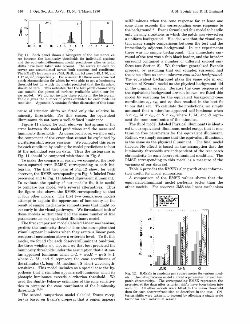
Fig. 11. Each panel shows a histogram of the luminance er-ror between the luminosity thresholds for individual sessionsand the equivalent-illuminant model predictions after criterionshifts have been taken into account. The errors for each ob-server are accumulated across both sessions and conditions.The RMSE’s for observers JMS, DHB, and KI were 0.49, 1.70, and1.17 cdym2, respectively. For observer KI there were some testpatch chromaticities for which he was able to set a luminositythreshold but for which the model predicted that the thresholdshould be zero. This indicates that the test patch chromaticitywas outside the gamut of surfaces realizable within our lin-ear model. We did not include these points in the histogram.Table 6 gives the number of points excluded for each modelingcondition. Appendix A contains further discussion of this issue.

cause of criterion shifts we fitted only the relative lu-minosity thresholds. For this reason, the equivalentilluminants do not have a well-defined luminance.

Figure 11 shows, for each observer, histograms of theerror between the model predictions and the measuredluminosity thresholds. As described above, we show onlythe component of the error that cannot be explained bya criterion shift across sessions. We computed this errorfor each condition by scaling the model predictions to bestfit the individual session data. Thus the histograms inFig. 11 should be compared with those in Fig. 8.

To make the comparison easier, we computed the root-mean-squared error (RMSE) corresponding to each his-togram. The first two bars of Fig. 12 show, for eachobserver, the RMSE corresponding to Fig. 8 (labeled Dataprecision) and to Fig. 11 (labeled Equivalent illuminant).To evaluate the quality of our model’s fit, it is usefulto compare our model with several alternatives. Thusthe figure also shows the RMSE corresponding to thatof four other models. The first two comparison modelsattempt to explain the appearance of luminosity as theresult of simple mechanistic computations that might oc-cur early in the visual pathways. We formulated both ofthese models so that they had the same number of freeparameters as our equivalent illuminant model.

The first comparison model (labeled Linear mechanism)predicts the luminosity thresholds on the assumption thatstimuli appear luminous when they excite a linear post-receptoral mechanism above a criterion level. To fit thismodel, we found (for each observer/illuminant condition)the three weights wL, wM , and wS that best predicted theluminosity thresholds under the assumption that a stimu-lus appeared luminous when wLL 1 wM M 1 wSS $ 1,where L, M , and S represent the cone coordinates ofthe stimulus (L, long-; M , medium-; S, short-wavelength-sensitive). This model includes as a special case the hy-pothesis that a stimulus appears self-luminous when itsphotopic luminance exceeds a criterion threshold. Weused the Smith–Pokorny estimates of the cone sensitivi-ties to compute the cone coordinates of the luminositythresholds.37,38

The second comparison model (labeled Evans recep-tor) is based on Evans’s proposal that a region appears

self-luminous when the cone response for at least onecone class exceeds the corresponding cone response tothe background.4 Evans formulated this model to handleonly viewing situations in which the patch was viewed ona uniform background. His idea was that the visual sys-tem made simple comparisons between the test and theimmediately adjacent background. In our experimentsthere was no simple background. The immediate sur-round of the test was a thin black border, and the broadersurround contained a number of different colored sur-faces (see Section 2). We therefore generalized Evans’sproposal by assuming that our complex surround hadthe same effect as some unknown equivalent background.The equivalent background plays the same role in ourversion of Evans’s model as the physical background didin the original version. Because the cone responses ofthe equivalent background are not known, we fitted thismodel by searching for the equivalent background conecoordinates cL, cM , and cS that resulted in the best fitto our data set. To calculate the predictions, we simplyassumed that a stimulus appeared self-luminous whenL $ cL, M $ cM , or S $ cS , where L, M , and S repre-sent the cone coordinates of the stimulus.

The third model (labeled Physical illuminant) is identi-cal to our equivalent-illuminant model except that it con-tains no free parameters for the equivalent illuminant.Rather, we simply assume that the equivalent illuminantis the same as the physical illuminant. The final model(labeled No effect) is based on the assumption that theluminosity thresholds are independent of the test patchchromaticity for each observer/illuminant condition. TheRMSE corresponding to this model is a measure of thevariance of our data set.

Table 6 provides the RMSE’s along with other informa-tion useful for model comparison.

A comparison of the RMSE values shows that theequivalent-illuminant model performs better than theother models. For observer JMS the linear-mechanism

Fig. 12. RMSE’s in candelas per square meter for various mod-els. The data-precision model allowed a parameter for each testpatch chromaticity. The corresponding RMSE represents theprecision of the data after criterion shifts have been taken intoaccount. All other models were fitted to the mean thresholddata for each observer/condition as described in the text. Cri-terion shifts were taken into account by allowing a single scalefactor for each individual session.


Table 6. Summary of Model Fitsa

Points

Subject Model Measured Fitted Parameter SSE RMSE

JMS Data precision 212 212 106 9 0.21Equivalent illuminant 212 212 21 52 0.49Linear mechanism 212 212 21 48 0.48Evans receptor 212 212 21 40 0.44Physical illuminant 212 212 6 86 0.64No model 212 212 6 247 1.08Constrained linear 212 212 16 60 0.53

DHB Data precision 214 214 114 229 1.03Equivalent illuminant 214 214 20 618 1.70Linear mechanism 214 214 20 1180 2.35Evans receptor 214 214 20 931 2.09Physical illuminant 214 214 5 1452 2.60No model 214 214 5 1536 2.68Constrained linear 214 214 15 668 1.77

KI Data precision 270 270 140 166 0.78Equivalent illuminant 270 264 20 364 1.17Linear mechanism 270 252 20 856 1.84Evans receptor 270 270 20 518 1.39Physical illuminant 270 268 5 2108 2.80No model 270 270 5 2008 2.73Constrained linear 270 265 15 405 1.24

aThe table provides the number of test patch chromaticities at which luminosity thresholds were obtained. The number of parameters for each modeltakes into account the criterion shift. For example, the equivalent-illuminant model has three free parameters for each illuminant condition. One ofthese parameters, however, is redundant to the criterion-shift scale factors. Thus for five illuminant conditions with two sessions per condition, theequivalent illuminant model has ten parameters to describe the five equivalent illuminants and ten parameters to describe the session-by-session criterionshifts. This corresponds to the 20 parameters listed for this model for observers DHB and KI. (Observer JMS ran one additional session, so for himthe model has 21 parameters.) Similar calculations lead to the parameter count for the other models.

and Evans-receptor models have slightly lower RMSE’sthan the equivalent-illuminant model, but for the othertwo observers the equivalent-illuminant model is substan-tially better. Of the models considered, the equivalent-illuminant, linear-mechanism, and Evans-receptormodels all have the same number of free parameters.Thus the RMSE values for these models are directlycomparable. The generally lower RMSE correspondingto the equivalent-illuminant model thus favors it overthe other two.

The physical-illuminant and no-effect models havehigher RMSE’s than the equivalent-illuminant modelbut have fewer parameters. Because these models arenot nested within the equivalent-illuminant model, thereis no easily applied goodness-of-fit test to decide whetherthe differences in RMSE are of statistical significance.(The physical illuminant generated by our apparatus isnot within the CIE linear model for daylights that weused to find the equivalent illuminant.) If we ignore thefact that the models are not nested, however, we can ap-ply an F -ratio goodness-of-fit test. We did so and foundthat we can reject the null hypothesis that the differencein RMSE is due to chance alone at the p , 0.001 levelfor all three observers. The F -ratios we obtained werefor JMS, F s15,191d 8.50; for DHB, F s15,194d 17.45;and for KI, F s15,250d 78.35. We applied the test asdescribed by Ashby and Lee.39 For observer KI the ap-plication of the test is complicated by the fact that notall of the measured points are within the model gamut.We corrected for this by assigning a squared error forthe out-of-model gamut points equal to the mean of the

squared error for the points that were in gamut. Thisissue is discussed at the end of Appendix A.

The equivalent-illuminant model fits better than theother models evaluated, but it does not describe the datato the measurement precision. Our data-precision mea-sure may be thought of as the RMSE for a model contain-ing a free parameter for every test patch chromaticity.To ask whether the difference between the equivalent-illuminant and the data-precision RMSE’s was due tochance alone, we applied an F -ratio goodness-of-fit test.Here the models are nested, as any prediction made bythe equivalent-illuminant model can be replicated by thedata-precision model. Again we were able to reject thehypothesis that the differences in RMSE were due tochance alone at the p , 0.001 level for JMS, at thep , 0.01 level for DHB, and at the p , 0.05 level for KI.The F -ratios obtained were for JMS, F s85,106d 5.98; forDHB, F s94,100d 1.81; and for KI, F s114,130d 1.35.We again corrected for KI’s out-of-gamut points duringperformance of this test. The fact that there is regular-ity in the data that is not described by the equivalent-illuminant model is also suggested by the plots of themodel fits shown in Figs. 4 and 5. Although the modelcaptures the qualitative features of the data, it missesin detail. One possible reason is that to fit the modelto the data, we had to choose specific linear models forsurface reflectances and illuminant spectral power dis-tributions. This a priori choice affects the model fits.As noted above, we did try some other combinations ofsurface and illuminant linear models. It seems likely,however, that some other choice of linear models would


provide a better fit, although how much better is diffi-cult to evaluate. Computational limitations prohibit anextensive search over the spaces of linear models.

B. Illuminant LinearityAlthough the equivalent-illuminant model does not pro-vide a complete description of the data, we believe that itcaptures enough of the variance to warrant its use for ad-dressing questions about how luminosity thresholds varywith the illumination. To demonstrate this, we investi-gate whether the equivalent illuminant depends linearlyon the physical illuminant. This is a hypothesis that hasbeen successfully used to understand how surface colorappearance varies with the illumination.40 The basicidea is as follows. Suppose that we measure equiva-lent illuminants E1sld and E2sld under two physicalilluminants E1sld and E2sld. If linearity holds, thenwhen the physical illuminant is any linear combination

Esld aE1sld 1 bE2sld (1)

(with a and b any scalars), the corresponding equivalentilluminant will be given by

Esld aE1sld 1 bE2sld (2)

for the same scalars a and b. The simplifying advan-tage of this illuminant linearity is that the equivalentilluminants corresponding to a wide range of physicalilluminants may be predicted from measurements of theequivalent illuminant for a small number of physicalilluminants. Since the equivalent illuminants in turnpredict the luminosity thresholds, illuminant linearityprovides the promise of a very compact description ofa large number of measurements. This sort of sim-plification is especially attractive because the rangeof naturally occurring illuminants may in fact be de-scribed as linear combinations of a small number of basisilluminants.17,18,32

Our five physical illuminants may be accurately de-scribed as a linear combination of two basis illuminants.That is, we can describe all of our experimental illumi-nants with Eq. (1), where E1sld, E2sld, and the five scalarpairs sa, bd are known. If linearity holds, we shouldbe able to find E1sld and E2sld such that when theyare used in Eq. (2) with the five scalar pairs sa, bd, weget equivalent illuminants that provide a good descrip-tion of our threshold data. For each observer we re-peated our search procedure with the added constraintthat the equivalent illuminants satisfy illuminant lin-earity. Adding the linearity constraint does not sub-stantially affect the RMSE error. Figure 13 comparesthe RMSE’s of the fits to the luminosity threshold datawith and without the linearity constraint. An F -ratiogoodness-of-fit test does, however, indicate that the dif-ference between the constrained and the unconstrainedfits is statistically significant ( p , 0.001 for JMS andKI, p , 0.01 for DHB). The F -ratios we obtained werefor JMS, F s5,191d 6.10; for DHB, F s5,194d 3.12; andfor KI, F s5,250d 5.34. Although this test indicatesthat illuminant linearity does not hold perfectly, we con-clude from the comparison of RMSE’s that the violation isvery small. Indeed, to the precision at which the uncon-strained equivalent-illuminant model describes the data,illuminant linearity holds quite well.

5. SUMMARY AND DISCUSSIONIn this paper we extended previous measurements of theperception of luminosity by having observers set luminos-ity thresholds under quite natural viewing conditions. Inaddition, we developed a physics-based model for lumi-nosity thresholds and showed that this model provides areasonable description of the data.

Our experiments show that observers can set lumi-nosity thresholds. A disappointing feature of our datais that there was considerable criterion shift across ses-sions (for some observers) and that the agreement amongobservers was poor. Perhaps a sharper specification ofthe observer’s task or more practice would allow col-lection of more consistent data. In his classic studies,Evans acted as his own primary observer and madefine distinctions among different forms of non-surface-mode appearance.6 – 8 We were initially hesitant to im-pose these distinctions on our observers, because theydid not strike us as natural at the time. A direction forfuture research clearly is to find methods for obtainingmore-precise measurements. It would also be useful tomodify our apparatus to allow measurements for a widergamut of chromaticities.

Our model generalizes previous methods for calculatingthe gamut of physically realizable surfaces (often calledoptimal surface stimuli) by including linear-model con-straints on the surface-reflectance functions.23,41 – 43 Forthis reason alone it may be of interest to color theo-rists, independent of its value for describing humanperformance. For example, the Deutsches Institut furNormung (DIN) color-order system uses optimal sur-face stimuli as a reference standard for determining thedarkness of colored samples.44 Our calculation providesa method to generate similar standards that take theregularities of natural surface-reflectance spectra intoaccount. Previously such regularities could be incorpo-

Fig. 13. RMSE’s for observers JMS, DHB, and KI with andwithout the linearity constraint. Both the general and theconstrained linear models were fitted to the mean thresholdsurfaces of each condition. For the constrained linear modelthe fitting procedure required the set of equivalent illuminantsto satisfy the illuminant-linearity constraint. The RMSE’s were0.49, 1.70, and 1.17 cdym2 without the linearity constraint and0.53, 1.77, and 1.24 cdym2 with the constraint for observers JMS,DHB, and KI, respectively.


rated only with brute-force methods, such as examiningthe physical gamut of a large set of measured samples.45

Our approach to understanding luminosity thresh-olds has much in common with the thinking of otherinvestigators. In his early work Evans comparedfluorence thresholds with the gamut of physically re-alizable surfaces under the illuminant specified by hisstimulus background.4 To make this comparison heused MacAdam’s method for computing the surfacegamut.23,41 – 43 This approach is essentially the oneimplemented in the physical-illuminant model above.The main difference is that we computed the surfacegamut under a linear-model constraint. Recall that thephysical-illuminant model did not provide a good fit to ourdata. Our equivalent-illuminant model extends Evans’sidea by allowing free parameters for the observer’s illumi-nant estimate. Ikeda and co-workers also used this gen-eral approach to model judgments of luminosity.11 Theycompared their data to the gamut of Munsell papers45

but found only approximate agreement. Like Evans,they did not allow for the possibility that the observermisestimated the illuminant.

A notion similar to that of our equivalent illuminantwas used recently by Bonato and Gilchrist10 to facilitateunderstanding of their measurements of achromatic lu-minosity thresholds. They found that luminosity thresh-olds varied with the physical illumination and that thethresholds were well predicted with a model that in-corporated a parameter to account for which stimulusthe observer judged to be white. This parameter playsthe same role in their thinking as the equivalent illu-minant does in ours. A similar approach has also beentaken by Ikeda and co-workers.12 Ullman’s9 approach tounderstanding luminosity thresholds was also in termsof a physics-based model. Rather than emphasizing ex-plicit estimates of surfaces and illuminants, however, heattempted to predict the thresholds on the basis of quan-tities that should be invariant in the absence of self-luminous objects.

One final approach has been used that aids in under-standing judgments such as ours. Evans and Swen-holt6 – 8 related their fluorence threshold data to measuresof the chromatic strength (e.g., saturation) of their teststimuli. They argued that these two types of appearancejudgment were mediated by the same visual mechanisms.We have not explored this intriguing idea, but to us it sug-gests the possibility that saturation might be understoodby consideration of a stimulus’s relation to the gamut ofphysically realizable surfaces.

One feature of our model may puzzle those familiarwith computational color constancy. In principle, boththe relative spectral power distribution and the abso-lute intensity of the equivalent illuminant play an im-portant role in our model calculations. Strictly speaking,however, the absolute intensity of the illuminant can betraded off against the absolute reflectance of the surfacesin the image. Halving the reflectance of every surfaceand doubling the illuminant intensity leaves the arrayof receptor responses unchanged. In light of this obser-vation it might seem unreasonable to suppose that thevisual system has any representation of the absolute il-luminant intensity. Recent computational approaches tocolor constancy, however, have employed Bayesian meth-

ods that incorporate probabilistic descriptions of whichsurfaces and illuminants are most likely to occur.30,46,47

In the Bayesian context it is possible to make a rea-sonable estimate both of the relative spectral power dis-tribution and of the overall illuminant intensity.46,47 Inpractice, we modeled only the relative shape of the lumi-nosity threshold surfaces. For this reason the absoluteintensity of the equivalent illuminant was undefined inour model fits. In the context of the above discussion,the criterion shifts that we observed could be interpretedas a consequence of uncertainty in the visual system’s es-timate of the absolute intensity of the illuminant.

Finally, it is worth noting that our equivalent-illumi-nant model has a character different from that of themore mechanistic models (i.e., the linear-mechanism andEvans-receptor models) with which we compared it. Ourmodel is based on the assumption that the visual sys-tem has internalized the physics of reflectance. It mod-els shifts in the luminosity thresholds with a calculationthat explicitly represents both linear-model and physical-realizability constraints on naturally occurring spectra.The comparison models, on the other hand, make no ref-erence to the nature of the external world. Rather, theyare based on the action of early visual mechanisms. Webelieve that a complete theory of luminosity thresholdsmust include both a mechanistic and a computational ex-planation. The superior fit of our equivalent-illuminantmodel suggests that to develop a mechanistic explanationwe may do well to consider how the action of visual mecha-nisms might approximate the calculations that our modelembodies.48

APPENDIX A: MODEL IMPLEMENTATIONTo implement our model, we require a method to cal-culate the luminosity threshold given an equivalent il-luminant. We will use the general linear-model-basedcolorimetric techniques described by Brainard.18 Let sbe an Nl-dimensional column vector whose entries spec-ify a surface reflectance function sampled at Nl evenlyspaced wavelengths throughout the visible spectrum.The vector s lies within an Ns-dimensional linear modelif we can write

s Bsws , (A1)

where Bs is a fixed Nl 3 Ns-dimensional matrix. Wecall Bs the basis matrix of the linear model; we call thecolumns of Bs the basis vectors of the linear model. Alinear model is specified completely by its basis matrix.Once a basis matrix for surface spectra has been cho-sen, we can specify any vector within the linear model byits vector of weights ws. In parallel fashion, let e be anNl-dimensional column vector whose entries specify illu-minant power sampled at Nl evenly spaced wavelengthsthroughout the visible spectrum. The vector e lies withinan Ne-dimensional linear model if we can write

e Bewe , (A2)

where Be is a fixed Nl 3 Ne-dimensional matrix. Inour calculations we assume that both surface and illu-minant spectra are constrained to lie within linear mod-


els and that the basis matrices for the two linear modelsare known.

Given a particular equivalent illuminant specified bywe (within the linear model defined by Be) and a testpatch chromaticity sx, yd, we must calculate the highestcolor-signal luminance consistent with a physically realiz-able surface within the linear model defined by Bs. Thiscan be cast as a linear programming problem. We seekto maximize a linear function of the weights ws subject tolinear equality and inequality constraints.

Let the 3 3 Nl-dimensional matrix T be the matrixwhose rows contain the CIE 1931 color-matching func-tions sampled at evenly spaced wavelengths throughoutthe visible spectrum, and let Ty be the Nl-dimensionalrow vector specifying the photopic luminosity function.The tristimulus coordinates r of the color signal reflectedfrom a surface ws under an illuminant we are given by

r T diagsBewedBsws , (A3)

where the expression diagsBewed indicates the diagonalmatrix with the entries of Bewe along its main diagonal.Similarly, the luminance Y of the color signal is given by

Y Ty diagsBewedBsws . (A4)

Equation (A4) implies that the stimulus luminance Y is alinear function of ws. We want to choose ws to maxi-mize the luminance subject to two constraints. First,the chromaticity of the color signal must be at a speci-fied value. Second, the surface reflectance function mustbe physically realizable. Both of these constraints maybe expressed as linear equality or inequality constraintson ws.

Let r0 be the unique tristimulus vector with unit lengthand chromaticity coordinates sx, yd. Let nullsr0d be a2 3 3 matrix whose rows form a basis set for the subspaceorthogonal to r0. The projection of r0 onto its orthogo-nal subspace is zero: nullsr0d r0 0. Any tristimulusvector r that satisfies nullsr0d r0 0 will have the samechromaticity sx, yd as r0, and all tristimulus vectors withchromaticity sx, yd satisfy nullsr0d r0 0. Thus we canexpress the chromaticity constraint as a linear constrainton ws:

nullsr0dT diagsBewedBsws 0 . (A5)

The constraints that the surface reflectance be physicallyrealizable are expressed as the linear inequalities

Bsws $ 0, Bsws # 1 . (A6)

Thus finding the maximum luminance consistent witha given equivalent illuminant we and color signal chro-maticity sx, yd is equivalent to the linear programmingproblem of finding the surface-weight vector ws that maxi-mizes the linear function of Eq. (A4) subject to the lin-ear constraints of Eqs. (A5) and (A6). We used the linearprogramming routine lp provided as part of the MATLAB

Optimization Toolbox to implement the maximization.49,50

To find the equivalent illuminant that provided the bestfit to the data, we implemented a numerical search proce-

dure over the equivalent illuminant we. For each choiceof we we computed the predicted luminosity thresholdsfor all test patch chromaticities, using the linear pro-gramming technique described above. This allowed usto compute the sum of squared errors between the dataand the prediction corresponding to any choice of we. Wesearched for the we that minimized this error.

One subtlety is worth noting. For some choices of we

and test patch chromaticity there will be no feasible solu-tion to the linear programming problem. In these casesthe model predicts that the test patch should appear lu-minous at any luminance. Physically this correspondsto the test patch chromaticity being outside the gamutof physically realizable surfaces that are within the lin-ear model defined by Bs. In computing the fit penalty inthis case, we took the predicted luminosity threshold tobe zero. This choice made the error for such points largeand tended to drive the search toward choosing equivalentilluminants for which all measured points were withingamut. In some cases, however, the final equivalent illu-minant resulted in out-of-gamut predictions for some testchromaticities. We excluded such points from the errorhistograms shown in Fig. 11. When we computed SSE’sand RMSE’s, we took the error for such points to be theaverage of the error for within-gamut points. This wasnecessary only for a small number of points for observerKI. We believe that it gives a more accurate picture ofmodel performance, since presumably small modificationsin the linear model for surfaces would have put all pointswithin gamut without drastically changing the overall fit.

ACKNOWLEDGMENTSWe thank L. Arend, M. D’Zmura, A. Gilchrist,K. Ishigami, A. T. Young, and an anonymous reviewerfor useful discussions and suggestions. We also thankJ. Tietz for his role in apparatus and software de-velopment. K. Ishigami observed in the experimentsreported here. P. Wise and L. Markan observed in pilotexperiments. This work was supported by National EyeInstitute grant EY10016.

REFERENCES AND NOTES1. D. H. Brainard, B. A. Wandell, and E.-J. Chichilnisky, “Color

constancy: from physics to appearance,” Curr. Dir. Psychol.Sci. 2, 165–170 (1993).

2. K. Buhler, “Gegenbemerkungen,” Psychol. Forsch. 5, 182–188 (1924), as discussed in Ref. 3.

3. G. Kreezer, “Luminous appearances,” J. Gen. Psychol. 4,247–281 (1930).

4. R. M. Evans, “Fluorescence and gray content of surface col-ors,” J. Opt. Soc. Am. 49, 1049–1059 (1959).

5. R. M. Evans, “Variables of perceived color,” J. Opt. Soc. Am.54, 1467–1474 (1964).

6. R. M. Evans and B. K. Swenholt, “Chromatic strength ofcolors: dominant wavelength and purity,” J. Opt. Soc. Am.57, 1319–1324 (1967).

7. R. M. Evans and B. K. Swenholt, “Chromatic strength ofcolors. Part II. The Munsell system,” J. Opt. Soc. Am. 58,580–584 (1968).

8. R. M. Evans and B. K. Swenholt, “Chromatic strength ofcolors. III. Chromatic surrounds and discussion,” J. Opt.Soc. Am. 59, 628–634 (1969).

9. S. Ullman, “On visual detection of light sources,” Biol. Cy-bern. 21, 205–212 (1976).


10. F. Bonato and A. L. Gilchrist, “The perception of luminosityon different backgrounds and in different illuminations,”Perception 23, 991–1006 (1994).

11. M. Ikeda, K. Motonaga, N. Matsuzawa, and T. Ishida,“Threshold determination for unnatural color appearancewith local illumination,” Kogaku 22, 289–298 (1993).

12. M. Ikeda, S. Fukumura, N. Matsuzawa, and T. Ishida, “In-fluence of surrounding visual information on the recognitionthreshold of local illumination,” Kogaku 23, 42–49 (1994).

13. Our usage of the term luminosity threshold follows that ofKreezer3 and of Bonato and Gilchrist.10 The term lumi-nosity is used in the literature both to describe physicalproperties of light14 and to describe perceptual experience.15

Ideal terminology would distinguish these two uses, but atpresent we feel that less confusion will be generated by ouruse of luminosity threshold than if we attempt to define newterminology.

14. D. L. MacAdam, Color Measurement: Theme and Varia-tions (Springer-Verlag, New York, 1981).

15. D. Judd and G. Wyszecki, Color in Business, Science, andIndustry (Wiley, New York, 1975).

16. R. N. Shepard, “The perceptual organization of colors: anadaptation to regularities of the terrestrial world?” in TheAdapted Mind: Evolutionary Psychology and the Genera-tion of Culture, J. H. Barkow, L. Cosmides, and J. Tooby,eds. (Oxford U. Press, New York, 1992).

17. CIE, Colorimetry, 2nd ed. (Bureau Central de la CIE, Paris,1986).

18. D. H. Brainard, “Colorimetry,” in Handbook of Optics:Vol. 1. Fundamentals, Techniques, and Design, M. Bass,ed. (McGraw-Hill, New York, 1995).

19. J. M. Speigle and D. H. Brainard, “Fluorescence thresholdsdepend on the illumination,” Invest. Ophthalmol. Vis. Sci.Suppl. 35, 1656 (1994).

20. L. T. Maloney and B. Wandell, “A computational model ofcolor constancy,” Invest. Ophthalmol. Vis. Suppl. 26, 206(1985).

21. M. D’Zmura and G. Iverson, “Color constancy. I. Basictheory of two-stage linear recovery of spectral descriptionsfor lights and surfaces,” J. Opt. Soc. Am. A 10, 2148–2165(1993).

22. E. Hering, “Der Raumsinn und die Bewegungen des Auges,”in Handbuch der Physiologie, B. L. Hermann, ed. (Vogel,Leipzig, 1879), Vol. 3, Part 1, as discussed in Ref. 3 above.

23. D. L. MacAdam, “The theory of the maximum visual effi-ciency of colored materials,” J. Opt. Soc. Am. 25, 249–252(1935).

24. A. L. Gilchrist, S. Delman, and A. Jacobsen, “The classifi-cation and integration of edges as critical to the perceptionof reflectance and illumination,” Percept. Psychophys. 33,425–436 (1983).

25. A. L. Gilchrist, “Lightness contrast and failures of constancy:a common explanation,” Percept. Psychophys. 43, 415–424(1988).

26. G. Buchsbaum, “A spatial processor model for object colourperception,” J. Franklin Inst. 310, 1–26 (1980).

27. D. H. Brainard and W. T. Freeman, “Bayesian method forrecovering surface and illuminant properties from photore-ceptor responses,” in Human Vision, Visual Processing, andDigital Display V, B. E. Rogowitz and J. P. Allebach, eds.,Proc. Soc. Photo-Opt. Instrum. Eng. 2179, 364–376 (1994).

28. D. Forsyth, “A novel algorithm for color constancy,” Int. J.Comput. Vision 5, 5–36 (1990).

29. G. D. Finlayson, “Color constancy in diagonal chromatic-ity space,” in Proceedings of the 5th International Confer-ence on Computer Vision (IEEE, Cambridge, Mass., 1995),pp. 218–223.

30. M. D’Zmura, G. Iverson, and B. Singer, “Probabilistic colorconstancy,” in Geometric Representations of Perceptual Phe-

nomena: Papers in Honor of Tarow Indow’s 70th Birthday,R. D. Luce, M. D’Zmura, D. Hoffman, G. Iverson, and A. K.Romney, eds., (Erlbaum, Hillsdale, N.J., 1995).

31. J. Cohen, “Dependency of the spectral reflectance curves ofthe Munsell color chips,” Psychon. Sci. 1, 369–370 (1964).

32. D. B. Judd, D. L. MacAdam, and G. W. Wyszecki, “Spectraldistribution of typical daylight as a function of correlatedcolor temperature,” J. Opt. Soc. Am. 54, 1031–1040 (1964).

33. L. T. Maloney, “Evaluation of linear models of surface spec-tral reflectance with small numbers of parameters,” J. Opt.Soc. Am. A 3, 1673–1683 (1986).

34. The other combinations of linear models we tried were(1) the CIE three-dimensional daylight model together witha three-dimensional linear model for the Munsell papers,(2) the CIE three-dimensional daylight model together witha six-dimensional linear model for the Munsell papers, and(3) a two-dimensional linear model for illuminants obtainedfrom a principal-components analysis of our experimental il-luminants together with the four-dimensional linear modelfor Munsell papers. These choices did not provide a betterfit than the combination we used. We evaluated only choice(2) on a subset of our data, because it was computationallyexpensive to compute the model fits for a six-dimensional-surface linear model.

35. K. L. Kelly, K. S. Gibson, and D. Nickerson, “Tristimulusspecification of the Munsell Book of Color from spectrophoto-metric measurements,” J. Opt. Soc. Am. 33, 355–376 (1943).

36. D. Nickerson, “Spectrophotometric data for a collection ofMunsell samples” (U.S. Department of Agriculture, Wash-ington, D.C., 1957; available from Munsell Color Company,Baltimore, Md.).

37. V. Smith and J. Pokorny, “Spectral sensitivity of the fovealcone photopigments between 400 and 500 nm,” Vision Res.15, 161–171 (1975).

38. P. DeMarco, J. Pokorny, and V. C. Smith, “Full-spectrumcone sensitivity functions for X-chromosome-linked anoma-lous trichromats,” J. Opt. Soc. Am. A 9, 1465–1476 (1992).

39. F. G. Ashby and W. W. Lee, “Predicting similarity and cate-gorization from identification,” J. Exp. Psychol. Gen. 120,150–172 (1991).

40. D. H. Brainard and B. A. Wandell, “Asymmetric color-matching: how color appearance depends on the illumi-nant,” J. Opt. Soc. Am. A 9, 1433–1448 (1992).

41. E. Schrodinger, “Theorie der pigmente von grossterLeuchtkraft,” Ann. Phys. 62, 603–622 (1920), as discussedin Ref. 50 below.

42. S. Rosch, “Die Kennzeichnung der Farben,” Phys. Z. 29,83–91 (1928), as discussed in Ref. 50 below.

43. G. Wyszecki and W. S. Stiles, Color Science—Concepts andMethods, Quantitative Data and Formulae, 2nd ed. (Wiley,New York, 1982).

44. M. Richter and K. Witt, “The story of the DIN color system,”Color Res. Appl. 11, 138–145 (1986).

45. M. R. Pointer, “The gamut of real surface colours,” ColorRes. Appl. 5, 145–155 (1980).

46. W. T. Freeman and D. H. Brainard, “Bayesian decision the-ory, the local mass estimate, and color constancy,” in Pro-ceedings of the 5th International Conference on ComputerVision (IEEE, Cambridge, Mass., 1995), pp. 210–217.

47. D. Marr, Vision, (Freeman, San Francisco, 1982).48. J. Little and C. Moler, MATLAB User’s Guide (The Math-

Works, Natick, Mass., 1991).49. A. Grace, Optimization Toolbox for Use with MATLAB User’s

Guide (The MathWorks, Natick, Mass., 1990).50. G. Wyszecki, “Color Appearance,” in Handbook of Perception

and Human Performance, K. R. Boff, L. Kaufman, and J. P.Thomas, eds. (Wiley, New York, 1986).

luminosity thresholds: effects of test chromaticity and...

Documents