Federal Reserve Bank of MinneapolisResearch Department

Lumpy Trade and Large Devaluations∗

George Alessandria, Joe Kaboski and Virgiliu Midrigan

April 2007

ABSTRACT

We document that trade flows, at the micro-economic level, are lumpy an infrequent; inventory-management problems faced by importers are more severe than those faced by firms that pur-chase material inputs domestically; and that a non-trivial component of international tradecosts is independent of a shipment’s size. We show that a parsimoniously parameterized(S, s)− type economy successfully accounts for these features of the data. We then show thatthe model predicts that, in response to a large increase in the relative price of imported goods,import values and the number of distinct imported varieties drops immediately, and as result,short-run import elasticities are substantially larger than long-run elasticities. The model alsopredicts that importers find optimal to reduce markups in response to the increase in thewholesale price of imports and thus partly rationalizes the slow increase in tradeable goods’prices following large devaluations. Our study of 6 current account reversals following largedevaluation episodes in the last decade provide strong support for the model’s predictions.

∗Author affiliations. The views expressed herein are those of the authors and not necessarily those of theFederal Reserve Bank of Minneapolis or the Federal Reserve System.

1. Introduction

How does a country’s current account respond to a devaluation? A large earlier literature1

motivated by the deterioration of the British and US current accounts following the 1967 and

1971 devaluations has argued that, because trade elasticities are lower (and in particular less

than unity) in the short-run than in the long-run, a devaluation may indeed initially dete-

riorate a country’s current account before improving it, thus exhibiting a J-curve response.

The following Wall Street Journal article, quoted by Magee (1973) summarizes this view:

The worsening U.S. trade deficit in the months after devaluation hasn’t really

been unexpected. Economists say that only in the long-run are international

trading patterns affected by new currency values. “Buying patterns don’t change

overnight because prices have changed,” a U.S. trade expert says.

This view is consistent with the findings of a growing recent literature in international

trade, as summarized, for example, by Ruhl (2005) and Yi (2003), that has emphasized that

trade elasticties estimated using high-frequency time-series data are centered around 0.5-1.5

and thus much lower than the cross-sectional elasticities in excess of 10 that are necessary to

rationalize the large response of trade volumes to trade liberalizations.

The recent sharp current account reversals experienced by Latin American and East

Asian economies in the aftermath of large devaluations and real exchange rate depreciations

appear thus puzzling in light of the evidence that international quantities respond slowly

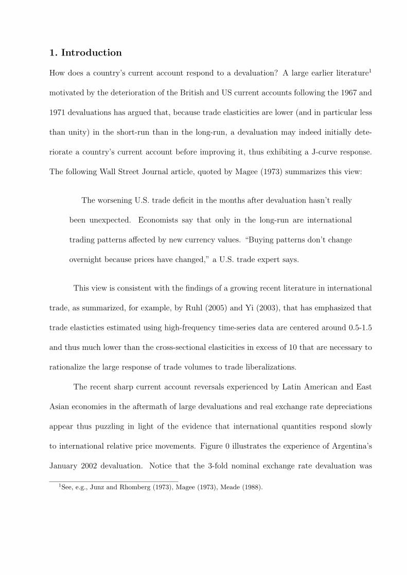
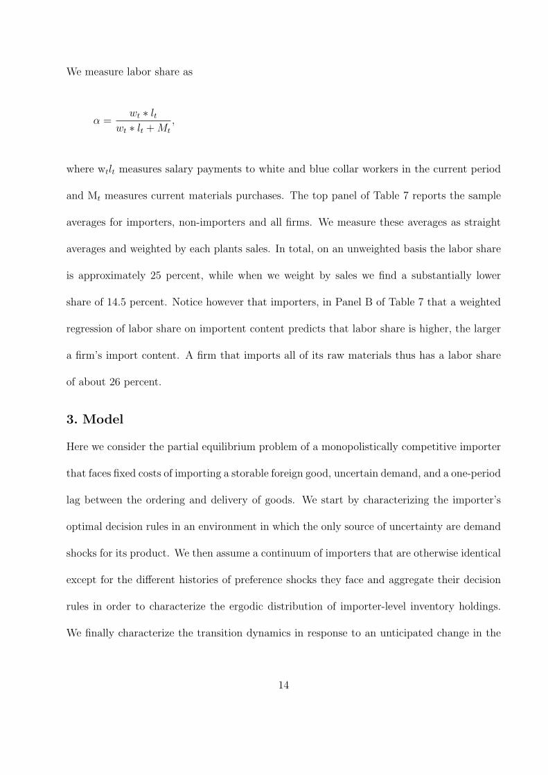
to international relative price movements. Figure 0 illustrates the experience of Argentina’s

January 2002 devaluation. Notice that the 3-fold nominal exchange rate devaluation was

1See, e.g., Junz and Rhomberg (1973), Magee (1973), Meade (1988).

associated with a 0.45 rise in the (log) relative price of (at-the-dock) imported goods to

the producer price index, a 1.4 drop in the dollar value of imports (implying an elasticity

of around 3, significantly higher than typical estimates of substitution elasticities based on

time-series data), and a negligible change in the value of exports. As a result the current

account sharply turned positive, with most of the increase driven by the high sensitivity of

imports to the relative price change.

We argue in this paper that two impediments to frictionless international trade can

account for this excess sensitivity of trade flows to relative price changes in the aftermath

of large devaluations. First, as forcefully documented by Hummels (2001), international

trade takes time: lags between orders and deliveries of goods are non-trivial. For instance,

shipments from Europe to the US Midwest take 2-3 weeks, those to Middle East as much as 6

weeks. Given demand uncertainty and depreciation of goods, these lags between orders and

delivery are non-trivial. Hummels estimates that an additional 30-day lag between orders

and delivers acts as a 12%-24% ad-valorem tax on a shipment’s value.

Longer distances are not the only factor contributing to the longer delays in trans-

actions associated with trading goods across borders. Man-made bureaucratic barriers are

a hinder as well. A recent survey by the World Bank2 finds that it takes an average of 12

days (OECD) to 37 days (Europe and Central Asia) for importers to assemble together im-

port licences, customs declaration forms, bills of lading, commercial invoices, technical and

health certificates, tax certificates and other certificates required to engage in international

transactions.

2Trading Across Borders. Available at http://www.doingbusiness.org/ExploreTopics/TradingAcrossBorders/

2

Second, a non-trivial component of the cost of international trade is fixed, that is,

independent of a shipment’s size. According to this same World Bank report, part of the

cost of importing a container into, say, Argentina, includes the cost of documents preparation

(750$), customs clearing and technical control (150$), as well as the cost of ports and terminal

handling (600$). These costs are arguably independent of a shipment’s size and thus provide

room for economies of scale in the transportation technology. We document in this paper

that these, and other fixed costs of international trade amount to 3%-11% of a shipment’s

value. Given that most goods transacted across borders are durable, these fixed costs would

make it optimal for importers to engage in international transactions infrequently and hold

non-zero inventories of imported goods.

We use two independent sources of evidence to document that importers indeed face

a non-trivial inventory-management problem. We first document that trade flows, at the

micro-economic level, are lumpy and infrequent. Using monthly data on the universe of all

US exports for goods in narrowly defined categories ( HS-10 ) against its trading partners,

we show that the average “good” is characterized by positive trade flows in only one half of

the months during a year, a statistic that overstates the frequency of trade at the good level

given that more than one good is typically included in an HS-10 category. Moreover, annual

trade is highly concentrated in a few months during the year. The bulk of trade (85%) is

accounted for by only 3 months of the year; the top month of the year accounts for 50% of

that year’s trade on average. Second, using a large panel of Chilean manufacturing plants,

we find that importing firms indeed hold roughly double the amount of inventories than firms

that only purchase raw materials domestically do.

3

These two frictions we emphasize imply that, at any point in time, importers hold

non-trivial amounts of inventories in order to economize on the fixed costs associated with

international trade, as well as in order to insure against unexpected changes in consumer

demand. A large, unexpected devaluation, which triggers a change in the relative price of

imported goods to the price of domestic firms the importers compete with, will render the

importer’s original holdings of inventories suboptimally high relative to what they would have

chosen given the higher market price of imports. As a result the fraction of firms (the extensive

margin) that import will drop immediately following the devaluation, thus exacerbating the

effect the relative price change has on a country’s import values. Indeed, as the lower-right

panel of Figure 0 indicates, the devaluation in Argentina coincides with a 2-fold decrease in

the number of varities imported in any given month, from 2000 prior to the crisis, to below

1000 in the aftermath of the devaluation.

Our goal is to quantitatively assess whether the two frictions discussed above, when

plausibly parameterized, can indeed account for the sharp current account reversals following

the devaluation. We embed these two trade frictions into a model with a continuum of mo-

nopolistically competitive importers that are subject to idiosyncratic demand shocks. These

frictions lead importers to follow an (S,s) rule in inventory holdings and importing. Thus

firms hold substantial inventories of imported goods throughout the year. The idiosyncratic

shocks lead to an ergodic distribution of inventory holdings across establishments. We choose

the parameters of the model to match the lumpiness of trade observed at the micro-level

and the inventory/purchases ratios observed in the Chilean panel of plant-level data. We

then study the response of our economy to large devaluations, modeled as changes in the

relative price of (at-the-dock) imported to domestic goods. Our main finding is that the

4

model predicts that short-run import demand elasticities are, as a result of fluctuations in

the extensive margin of trade (# of imported varieties) 4-times larger than long-run elas-

ticities implied by consumer’s Arminton elasticity for imported goods. The model can thus

successfuly rationalize the sharp drop in import values following large devaluations.

Moreover, the model also generates import price dynamics that are consistent with

the evidence documented by Burstein et al. (2005) for large devaluations that tradable

goods prices, at the retail level, respond increase despite the fact that at the-dock prices of

imported goods rise almost one-for-one to the nominal exchange rate changes. In particular,

importers in our model find it optimal to lower markups charged to consumers following the

devaluations by increasing retail prices slowly in response to the change in the wholesale

price of imported goods. This imperfect pass-through arises because after the devaluation

importers find themselves overstocked with imported goods at the current replacement price.

If importers were to fully pass-through the price change, they would hold onto their imports

for a long time and substantially increase their inventory carrying costs. Instead, to economize

on inventory holding costs, they find optimal to partially increase their price. As inventory

holdings are depleted, and firms return to the import market, more firms increase their prices

and pass-through rises with time.

This paper brings together three distinct lines of research. First, a number of authors

have studied non-convexities of inventory adjustment over the business cycle in partial (Caplin

1985, Caballero and Engel 1991) and general equilibrium environments (Fisher and Hornstein

2000, Khan and Thomas 2007). Unlike these papers which focus on relatively small shocks our

emphasis is on large aggregate shocks. Second, our focus on emerging markets business cycles

is similar to Neumeyer and Perri (2005) and Aguiar and Gopinath (2007). However, unlike

5

these GE studies, we develop a partial equilibrium model and study only import dynamics

in the aftermath of large devaluations. Third, a number of recent papers study changes in

the extensive margin around trade liberalizations (Ruhl (2005)) and over the business cycle

(Alessandria and Choi (2007) and Ghironi and Melitz (2005)). Unlike these papers, which

focus on sunk costs of participating in international trade, we emphasize the storability of

internationally-traded goods and the economies of scale associated with international trade.

Finally, the literature measuring trade costs, summarized by Anderson and Van Wincoop (),

finds large costs of international trade with tariff equivalents of nearly 140 (check) percent.

We extend the range of costs considered to include the fixed costs of importing the lags

between orders and delivery in international trade.

2. Data

This section uses microdata to document several important and related facts of importing

behavior: (i) the lumpiness of trade shipments, (ii) the fixed costs of trading, and (iii) the

relationship between inventories (both final goods and materials) and import content. We

focus on data for developing countries in documenting these facts, and address each fact in

sequence.

A. Lumpiness of International Transactions

We document the lumpiness of international transactions using monthly data from January,

1990 to April, 2005 on U.S. exports to six importing countries that have experienced large de-

valuations during this period: Argentina (2002), Brazil (1999), Korea (1997), Mexico (1994),

Russia (1998), and Thailand (1997). The data is comprehensive of U.S. goods exports over

the period and is highly disaggregate (over 10,000 commodities at 10-digit Harmonized Sys-

6

tem codes) and includes monthly totals of exported quantity, value, and number of individual

transactions by destination country and exiting district. We define a good to be a distinct

HS code commodity exiting a particular district, and look at the lumpiness of monthly trade

flows of these goods to each country.

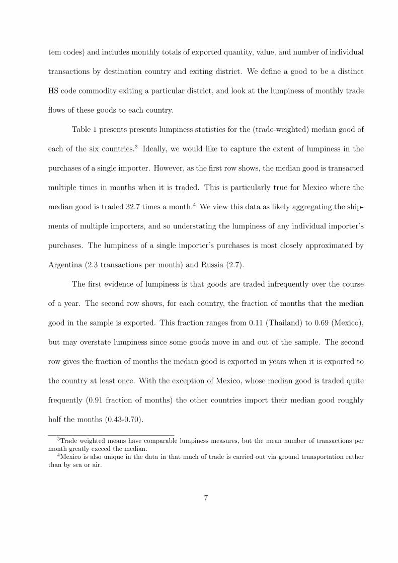
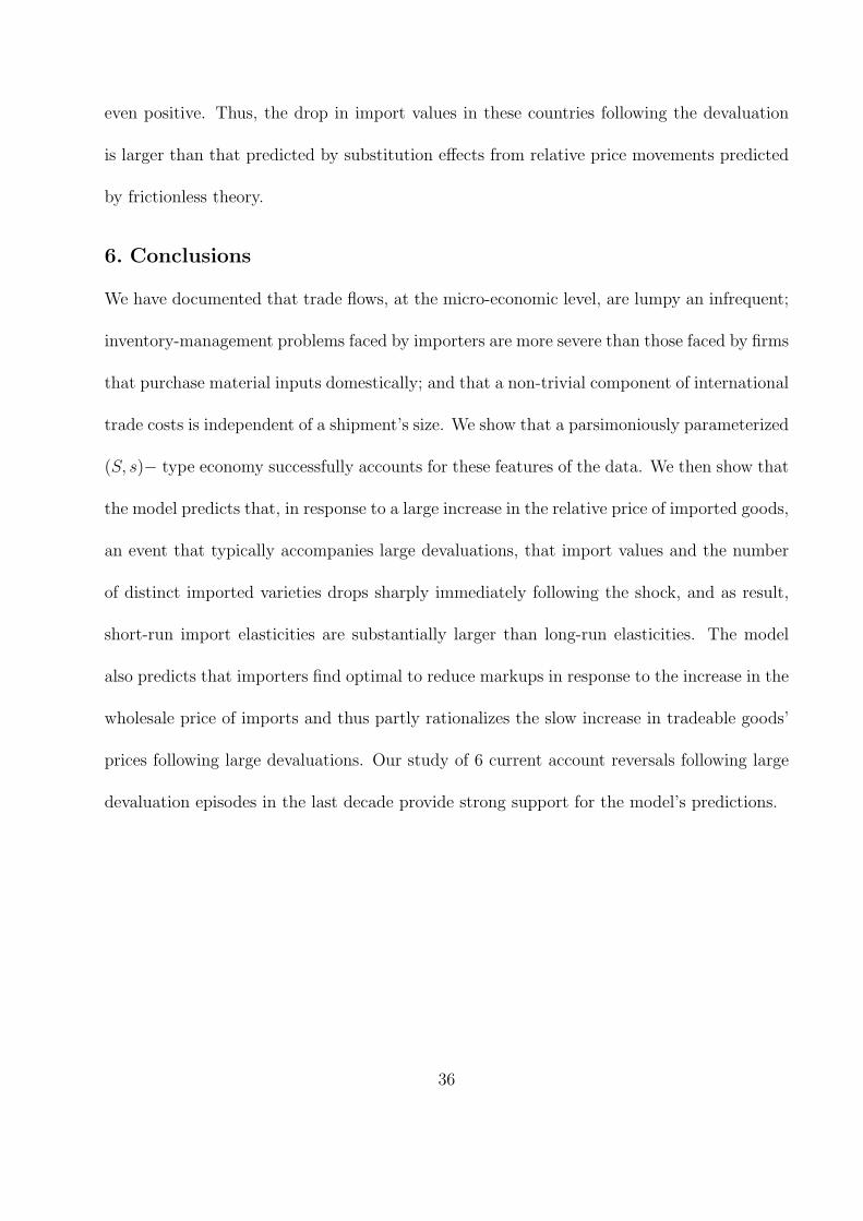
Table 1 presents presents lumpiness statistics for the (trade-weighted) median good of

each of the six countries.3 Ideally, we would like to capture the extent of lumpiness in the

purchases of a single importer. However, as the first row shows, the median good is transacted

multiple times in months when it is traded. This is particularly true for Mexico where the

median good is traded 32.7 times a month.4 We view this data as likely aggregating the ship-

ments of multiple importers, and so understating the lumpiness of any individual importer’s

purchases. The lumpiness of a single importer’s purchases is most closely approximated by

Argentina (2.3 transactions per month) and Russia (2.7).

The first evidence of lumpiness is that goods are traded infrequently over the course

of a year. The second row shows, for each country, the fraction of months that the median

good in the sample is exported. This fraction ranges from 0.11 (Thailand) to 0.69 (Mexico),

but may overstate lumpiness since some goods move in and out of the sample. The second

row gives the fraction of months the median good is exported in years when it is exported to

the country at least once. With the exception of Mexico, whose median good is traded quite

frequently (0.91 fraction of months) the other countries import their median good roughly

half the months (0.43-0.70).

3Trade weighted means have comparable lumpiness measures, but the mean number of transactions permonth greatly exceed the median.

4Mexico is also unique in the data in that much of trade is carried out via ground transportation ratherthan by sea or air.

7

Mere frequency of trade also understates the degree of lumpiness, however, because

most of the value of trade is concentrated in still fewer months. One way of summarizing this

concentration is by using the Herfindahl-Hirschman (HH) index. The HH index is defined

as follows:

HH =12∑i=1

s2i

where si is the share of annual trade accounted for by month i. The index ranges 1/12 (equal

trade in each month) to one (all trade concentrated in a single month). If annual trade were

distributed equally across n months in a year, then the HH would equal 1/n. The HH indexes

for all countries but Mexico range 0.26 to 0.45. If all trade were equally distributed across

months, these number would translate into roughly 2 to 4 shipments per year.

Finally, the last three rows another measure of concentration, the fraction of annual

trade accounted for by the months with the highest trade in a given year for the median

good. The numbers show that the top month accounts for a sizable fraction (ranging from

0.36-0.53, excluding Mexixo), while the top 3 months account for the vast majority of trade

(0.70-0.85), and the top five months account for nearly all of annual trade (0.86-0.95).

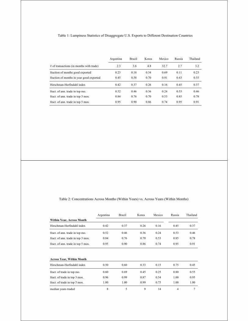
This high level of concentration does not appear to be driven by seasonalities. This

is shown in Table 2. The top half of the table reproduces the HH index and fraction of

trade numbers from Table 1, where the fractions are the fraction of trade in a given year.

The numbers in the bottom half reproduce the analogous numbers for the fraction of trade

in a given month (e.g., December) across years in the data. For these numbers, trade is

normalized by annual trade to prevent concentrations from developing by secular changes in

8

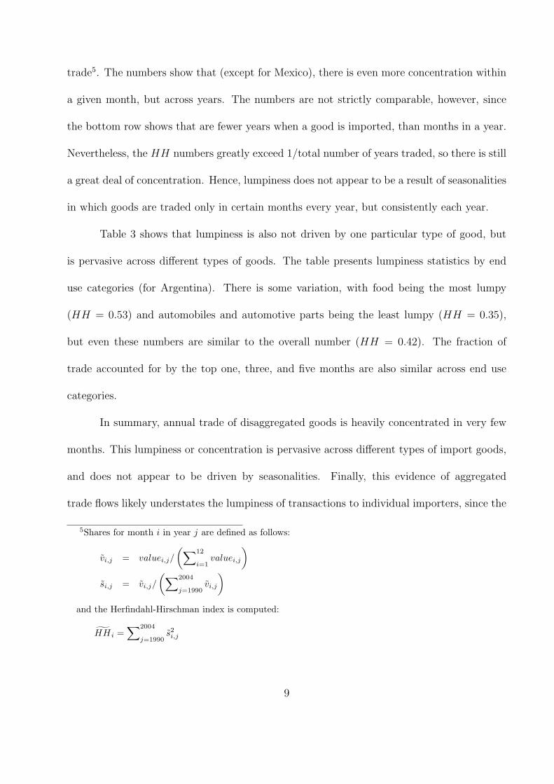
trade5. The numbers show that (except for Mexico), there is even more concentration within

a given month, but across years. The numbers are not strictly comparable, however, since

the bottom row shows that are fewer years when a good is imported, than months in a year.

Nevertheless, the HH numbers greatly exceed 1/total number of years traded, so there is still

a great deal of concentration. Hence, lumpiness does not appear to be a result of seasonalities

in which goods are traded only in certain months every year, but consistently each year.

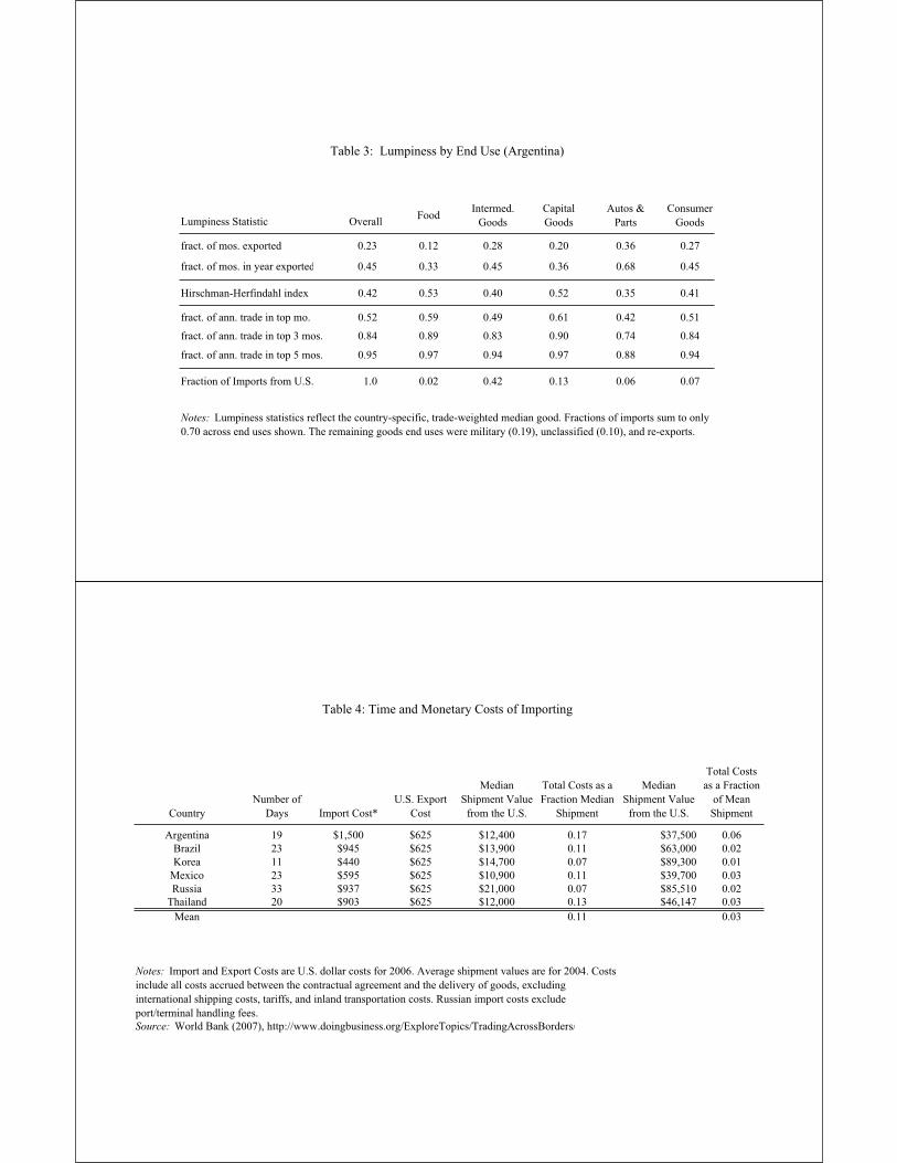
Table 3 shows that lumpiness is also not driven by one particular type of good, but

is pervasive across different types of goods. The table presents lumpiness statistics by end

use categories (for Argentina). There is some variation, with food being the most lumpy

(HH = 0.53) and automobiles and automotive parts being the least lumpy (HH = 0.35),

but even these numbers are similar to the overall number (HH = 0.42). The fraction of

trade accounted for by the top one, three, and five months are also similar across end use

categories.

In summary, annual trade of disaggregated goods is heavily concentrated in very few

months. This lumpiness or concentration is pervasive across different types of import goods,

and does not appear to be driven by seasonalities. Finally, this evidence of aggregated

trade flows likely understates the lumpiness of transactions to individual importers, since the

5Shares for month i in year j are defined as follows:

vi,j = valuei,j/

(∑12

i=1valuei,j

)si,j = vi,j/

(∑2004

j=1990vi,j

)and the Herfindahl-Hirschman index is computed:

HHi =∑2004

j=1990s2

i,j

9

monthly data contains multiple transactions, that likely reflect multiple purchasers.

One potential reason for this lumpiness is the presence of fixed shipping costs in

international trade. We turn now to this evidence.

B. Fixed Costs of International Transactions

A related salient characteristic of international trade are the sizable fixed costs of trade,

both in terms of time costs and monetary costs. Data on these costs are available from the

World Bank’s Doing Business database (World Bank, 2007)6. These costs are comprehensive

of all costs accrued between the contractual agreement and the delivery of goods, excluding

international shipping costs, tariffs, and inland transportation costs.7 They include document

preparation, customs clearing/technical control, and port/terminal handling faced by both

the exporting and importing country.8

Table 4 summarizes the costs faced for different countries. The first column shows

that time costs are considerable. Importing time costs range from 11 (Korea) to 33 (Russia)

days, but roughly three weeks is the norm in the other countries.9 These costs exclude inland

transportation on both sides (typically 2 days in the U.S. and 2 days in the destination

country), and shipping costs are on the order of a couple of weeks for boats, which is the

most common shipping form in the U.S. export data for all but Mexico. Thus, a typical

6See Djankov et. al. (2006) for a description of the survey methodology underlying this data.7The costs are based on a standardized container of cargo of non-hazardous, non-military textiles, apparel,

or cofee/tea/spice between capital cities. We exclude inland transportation costs on both sides, since thesecosts may not be specific to international trade.

8Common import documents include bills of lading, commercial invoices, cargo manifests, customs cargorelease forms, customs import declaration forms, packing lists, shipment arrival notices, and quality/healthinspection certificates. U.S. export documents consist of a bill of lading, certificate of origin, commercialinvoice, customs export declaration form, packing list, and pre-shipment inspection clean report of findings.

9Exporting time costs from the U.S. are roughly a week, but we exclude these since we assume that thisis concurrent with the import time costs in the destination country.

10

shipment takes one to two months from the time of order to receipt of goods.

The second and third columns show the importing and exporting costs respectively.

These costs are in U.S. dollars for 2006, and we view most costs as predominantly fixed

costs. Importing costs are roughly $500 for Mexico and Korea, $1000 for Brazil, Russia,

and Thailand, and $1500, while U.S. export costs are an additional $625.10 The median

shipments in 2004 from the U.S. export data are in the range of $10,900 (Mexico) to $21,000

(Russia), while average shipments are much larger, ranging between $37,500 (Mexico) to

$89,000 (Korea). Based on these data, importing and exporting costs as a fraction of median

shipments range from 0.07 to 0.17, and 0.01 to 0.06 as a fraction of mean shipments.

These costs omit international shipping costs which are also non-neglible. U.S. import

data (the counterpart of the export data) contain freight charges for similar sized shipments.

These data indicate that freight costs between the U.S. and these countries range from $500

(South Korea) to $1000 (Argentina and Brazil), with Mexico being the one exception ($100)

because of the prevalence of trucking. Freight costs contain a substantial fixed cost compo-

nent, driven in part by containerized shipping technology which greatly increases the per unit

costs of shipping less than a full container.

C. Evidence from Chilean plant-level data

Our evidence on lumpy trade suggests establishment face inventory management consider-

ations when purchasing goods internationally. However, this is only indirect evidence. For

more direct evidence on the relation between inventory and importing, we use plant-level

data on inventories and the source of production inputs. For this we turn to a panel of

10Russian import costs omit port/terminal handling charges.

11

Chilean manufacturing plants. The data covers 7 years (1990 to 1996) and includes 7,234

unique plants and 34,990 observations. This panel has been studied extensively elsewhere (see

Roberts and Tybout 1996). The plant-level data is well suited for our purposes as Chile is at

a comparable level of economic development to the countries that experienced devaluations

and thus Chilean plants are more likely to be similar to plants in these countries.

For each plant j, we have data on beginning and end of year inventories broken down

by materials(Imjt+1, I

mjt

)and goods in process (If

jt+1, Ifjt) as well as annual material purchases,

Mjt, sales, Yjt and materials imports, M imjt . We define inventories as the average of beginning

and end of period inventories, or If

jt = (Ifjt+1 + If

jt)/2 and Im

jt = (Imjt+1 + Im

jt ). We measure

the import content as the share of materials imported or simjt = M im

jt /Mjt. To measure each

plant’s inventory turnover we divide each type of inventory holding by its annual use. For

materials, we define the inventory holdings relative to annual purchases imjt = (Im

jt/Mt) while

for finished goods inventories we divide these by annual sales ifjt = (If

jt/Yt). Our measure

of finished inventories reflects the materials content of final goods. The total investment in

inventories is denoted by ijt = imjt + ifjt.

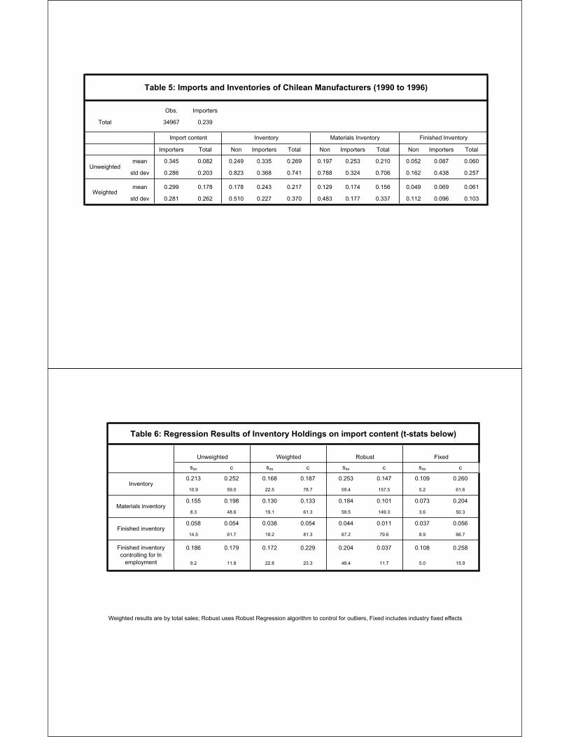
Table 5 reports some summary statistics from this panel of manufacturing plants for

the whole period for our three different measures of inventory holdings.11 We report both un-

weighted averages and averages weighted by annual sales. For the sake of brevity we discuss

only the unweighted averages reported in the top panel. On average, the typical manufac-

turing plant holds approximately 28.5 percent of its annual purchases in inventories. Among

non-importers, the typical plant holds 26.2 percent of its annual purchases in inventories while

11Over the sample, about 24 percent of our plants imported in a particular year. Over time the share ofimporters in the sample increases by approximately ten percent.

12

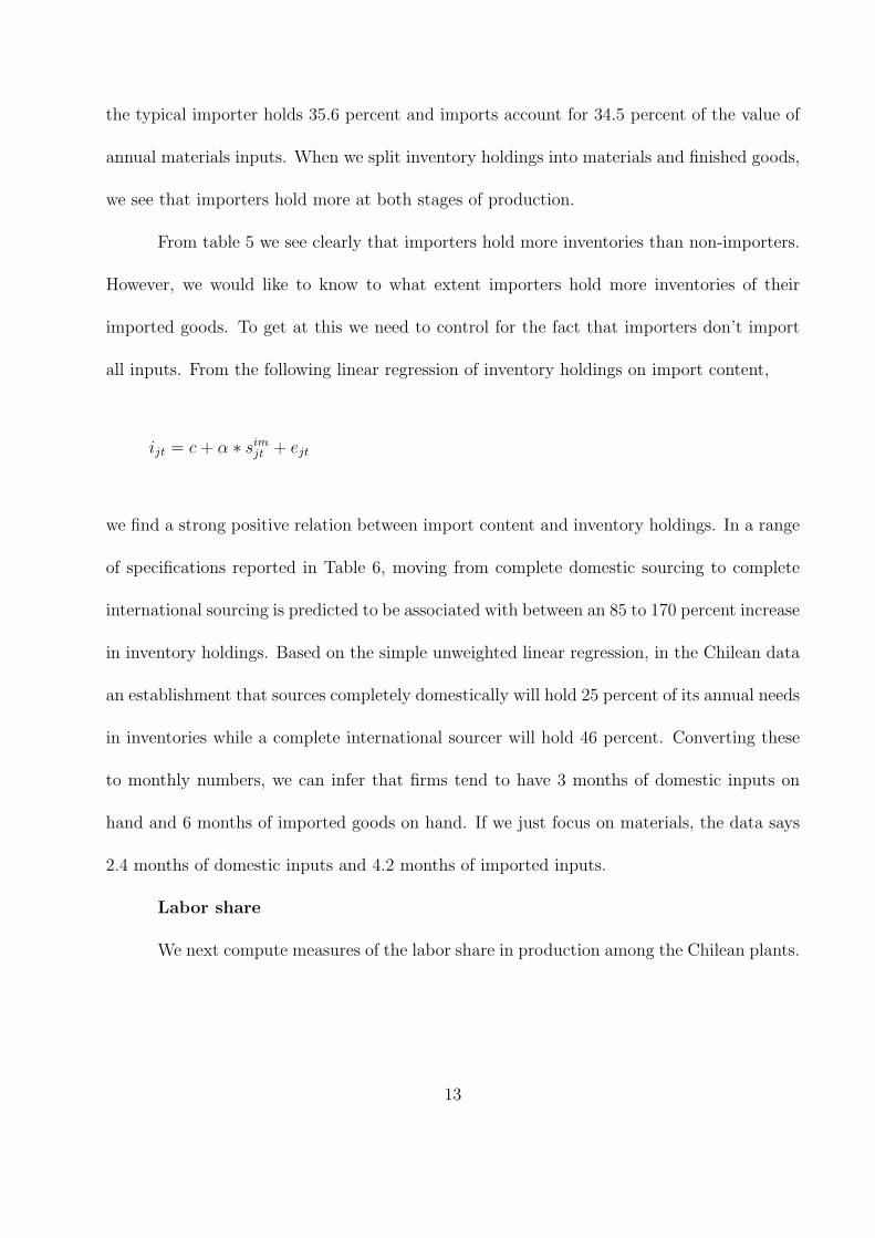
the typical importer holds 35.6 percent and imports account for 34.5 percent of the value of

annual materials inputs. When we split inventory holdings into materials and finished goods,

we see that importers hold more at both stages of production.

From table 5 we see clearly that importers hold more inventories than non-importers.

However, we would like to know to what extent importers hold more inventories of their

imported goods. To get at this we need to control for the fact that importers don’t import

all inputs. From the following linear regression of inventory holdings on import content,

ijt = c + α ∗ simjt + ejt

we find a strong positive relation between import content and inventory holdings. In a range

of specifications reported in Table 6, moving from complete domestic sourcing to complete

international sourcing is predicted to be associated with between an 85 to 170 percent increase

in inventory holdings. Based on the simple unweighted linear regression, in the Chilean data

an establishment that sources completely domestically will hold 25 percent of its annual needs

in inventories while a complete international sourcer will hold 46 percent. Converting these

to monthly numbers, we can infer that firms tend to have 3 months of domestic inputs on

hand and 6 months of imported goods on hand. If we just focus on materials, the data says

2.4 months of domestic inputs and 4.2 months of imported inputs.

Labor share

We next compute measures of the labor share in production among the Chilean plants.

13

We measure labor share as

α =wt ∗ lt

wt ∗ lt + Mt

,

where wtlt measures salary payments to white and blue collar workers in the current period

and Mt measures current materials purchases. The top panel of Table 7 reports the sample

averages for importers, non-importers and all firms. We measure these averages as straight

averages and weighted by each plants sales. In total, on an unweighted basis the labor share

is approximately 25 percent, while when we weight by sales we find a substantially lower

share of 14.5 percent. Notice however that importers, in Panel B of Table 7 that a weighted

regression of labor share on importent content predicts that labor share is higher, the larger

a firm’s import content. A firm that imports all of its raw materials thus has a labor share

of about 26 percent.

3. Model

Here we consider the partial equilibrium problem of a monopolistically competitive importer

that faces fixed costs of importing a storable foreign good, uncertain demand, and a one-period

lag between the ordering and delivery of goods. We start by characterizing the importer’s

optimal decision rules in an environment in which the only source of uncertainty are demand

shocks for its product. We then assume a continuum of importers that are otherwise identical

except for the different histories of preference shocks they face and aggregate their decision

rules in order to characterize the ergodic distribution of importer-level inventory holdings.

We finally characterize the transition dynamics in response to an unticipated change in the

14

relative price of imported to domestically produced goods. We consider both permanent and

temporary changes in this relative price.

Formally, we consider a small-open economy inhabited by a large number of identical,

infinitely-lived importers, indexed by j. In each period t, the importer experiences one of

infinitely many events, ηt. Let ηt = (η0, ..., ηt) denote the history of events up to period t.

Let pj(ηt) denote the price charged by importer j in state ηt and νj(η

t) denote the

importer-specific demand disturbance. νj(ηt) is assumed iid across firms and time. We

assume a static, constant-elasticity of substitution demand specification for the importer’s

product12:

yj(ηt) = νj(η

t)pj(ηt)−θ

Let ωj = ω be the wholesale per-unit cost of imported goods, assumed constant across

all importers. We will interpret changes in ω as changes in the relative price of (at-the-dock)

imported goods to that of domestic goods. In addition, we assume that the importer faces

an additional, fixed cost of importing f , every period in which it imports. Given that the

imported good is storable, the firm will find it optimal to import infrequently and carry non-

zero holdings of inventories from one period to another. Let sj(ηt) be the stock of inventory

the importer starts with at the beginning of the period at history ηt. Given this stock of

inventory, the firm has two options: pay the fixed cost f and import ij(ηt) > 0 new units

12In the background we have in mind a consumer that has preferences over Foreign and Home goods:

c =(h

θ−1θ + γ

∫ 1

0ν

1θj m

θ−1θ

i di) θ

θ−1where mi is consumption of imported good j, h is consumption of the

domestic good and γ, the weight on imported goods is assume to be close to 0. Normalizing the price of homegoods to 1 would yield the demand functions in text.

15

of inventory; or save the fixed cost and not import, i.e., set ij(ηt) = 0. Implicit in this

formulation is the assumption that inventory investment is irreversible, i.e., re-exports of

previously imported goods, ij(ηt) < 0 are ruled out.

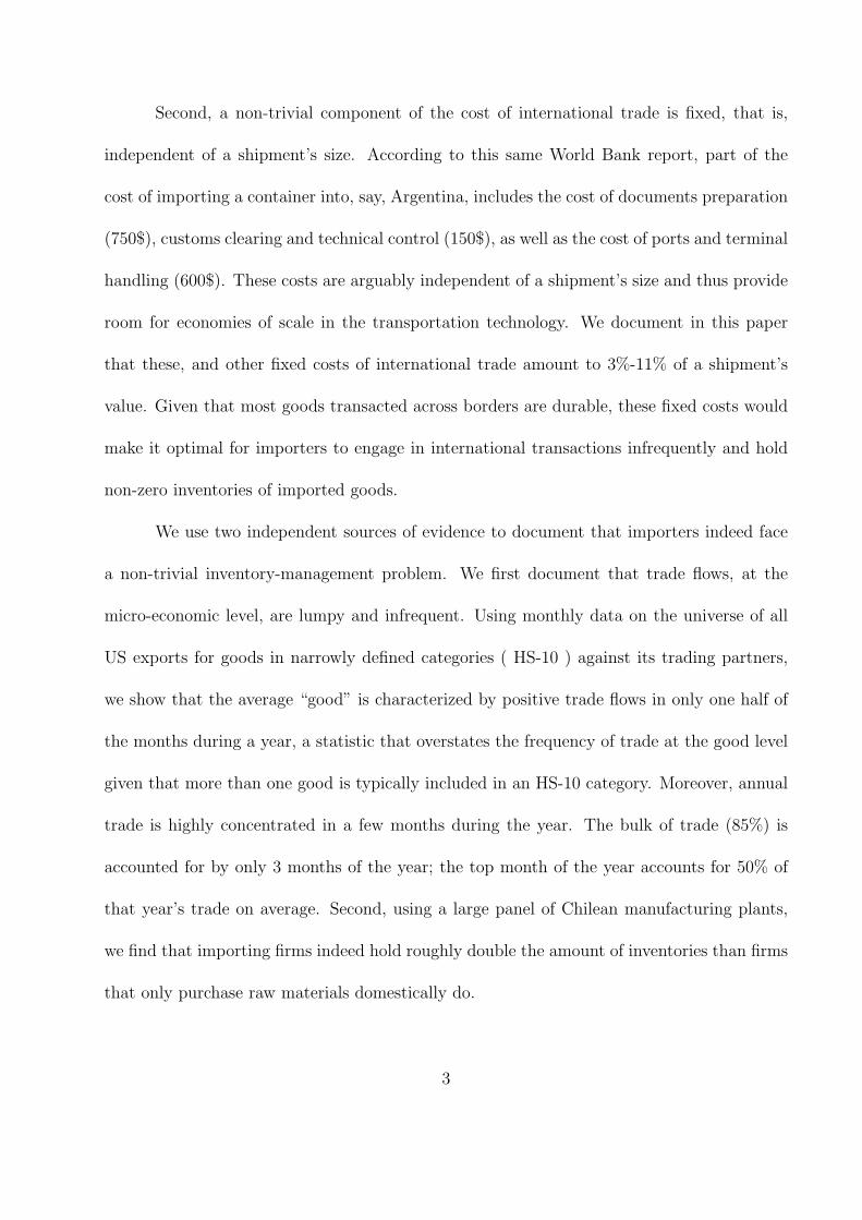
We also assume a one-period lag between orders of imports and delivery. That is, sales

of the importer at ηt, qj(ηt) are constrained to not exceed the firm’s beginning-of-period stock

of inventory:

qj(ηt) = min[νj(η

t)pj(ηt)−θ, sj(η

t)]

The amount ij(ηt) the importer orders today can be only used for sales next period.

In particular, the law of motion for the importer’s beginning of the period inventories is:

sj(ηt+1) = (1− δ)

[sj(η

t)− qj(ηt) + ij(η

t)]

where δ is the depreciation rate. We assume that inventory in transit ij(ηt), depreciates at

the same rate as inventory in the importer’s wharehouse, sj(ηt)−qj(η

t). Figure 1 summarizes

the timing assumptions in the model.

The firm’s problem can be concisely summarized by the following system of two func-

tional Bellman equations. Let V a(s, ν) denote the firm’s value of adjusting its stock of

inventory and V n(s, ν) denote the value of inaction, as a function of its beginning-of-period

stock of inventory and its demand shock. Let V (s, ν) = max[V a(s, ν), V n(s, ν)] denote the

16

firm’s value. Then the firm’s problem is:

V a(s, ν) = maxp,i>0

q(p, s)p− ωi− f + βEV (s′, ν ′)(1)

V n(s, ν) = maxp

q(p, s)p + βEV (s′, ν ′)

where

q(p, s) = min(νp−θ, s)

and

s′ = (1− δ) [s− q(p, s) + i] if adjust

s′ = (1− δ) [s− q(p, s)] if don’t adjust

The expectations on the right-hand sides of the Bellman equations are taken with

respect to the distribution of demand shocks ν. We assume log(ν) ∼ N(0, σ2).

A. Optimal policy rules

We next characterize the optimal decision rules for the firm’s problem13. In particular, we

are interested in characterizing pa(s, ν), pn(s, ν), the prices the firm charges conditional on

adjusting or not its inventory holdings, i(s, ν), the firm’s purchases of inventory conditional

on importing, as well as φ(s, ν), the firm’s binary adjustment decision.

13We solve this problem numerically, using spline polynomial approximations to approximate the 2 valuefunctions, and Gaussian quadrature to compute the integrals on the right-hand-side of the Bellman equations.Details are available from the authors upon request.

17

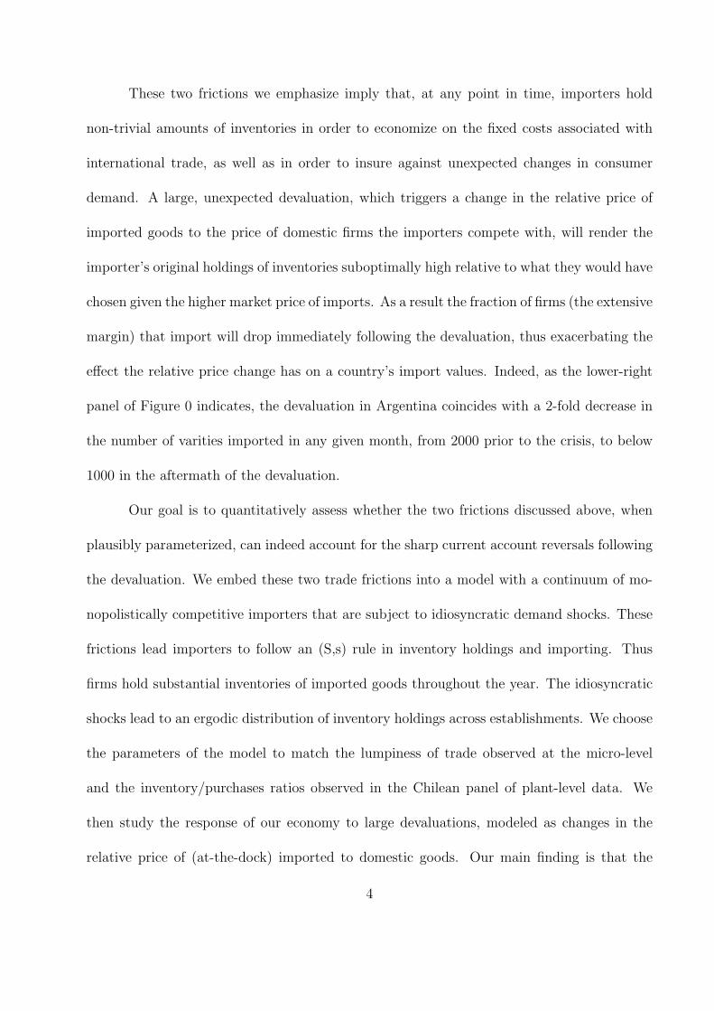
Figure 2 depicts the firm’s values of adjusting and not adjusting its inventory in the s

(beginning-of-period stock of inventories) space. The second argument of these functions is

held constant at its steady-state level.

Note that both values are concave in the importer’s level of inventory. In this model

an increase in s raises the firm’s value for 3 reasons: it reduces the probability of a stockout,

i.e., the probability that the firm will have insufficient inventories to meet all demand; it

reduces the probability that the firm will have to pay the fixed importing cost next period,

as well as directly, by raising the value of the firm’s assets. Whenever the firm has little

inventories, the likelihood of a stockout is high, and, conditional on inaction, the probability

of adjustment next period is high as well, hence the firm’s value rises faster with s than when

the firm has higher levels of inventories. Notice also in this region that the firm that does

not adjust values an additional unit of inventory more than the firm that does adjust. Given

our assumed lag between orders and deliveries, the choice of not adjusting today implies that

the firm will have to sell out of its current (low) stock of inventory not only today, but also

next period, thus making each additional unit of inventory today more valuable.

The intersection of these two functions define the firm’s inaction region. Whenever its

stock of inventory is too low, the firm orders a new batch of inventories and pays the fixed

cost f . Similarly, whenever the firm has a sufficiently high stock of inventories it prefers to

postpone ordering, thus saving the fixed cost.

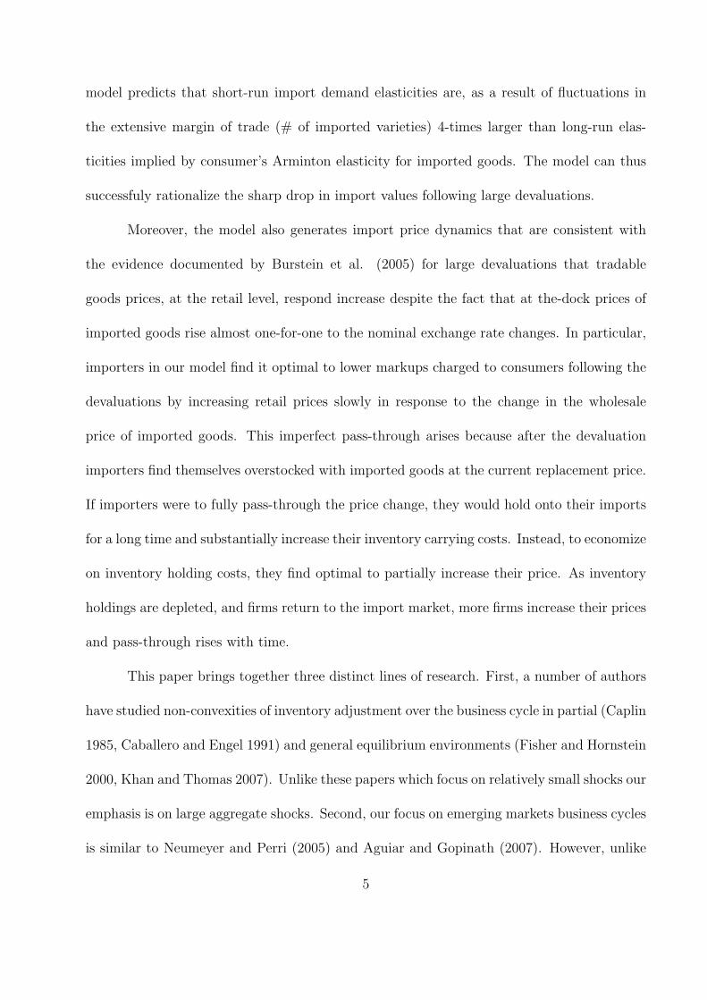
We next turn to the optimal price functions, illustrated in Figure III. Clearly, whether

the firm orders or not new inventories affects its next period’s beginning of period’s inventories

and thus its marginal valuation of an additional unit of inventory, reflected in the firm’s price.

Consider first the pa(s, ν) schedule, the firm’s price, conditional on ordering new inventories.

18

Again, we supress the ν argument in this figure and set the level of demand to its steady-state

mean. Notice that pa(s) initially decreases with s, then flattens out, and then decreases again

when s is sufficiently high. The first portion of this schedule is one where s is sufficiently low

for the firm to not be able to meet demand if it charges the price that would be optimal in

the absence of the constraint that firm’s sales must not exceed its inventory. The importer

thus charges a price that ensures that it sells all of its currently available inventory. The

firm’s price in this region is implicitly defined by:

vp−θ = s

Consider next the second, flat region. If the firm does not stock out and adjusts its inventory,

its price next period is independent of current inventories for most of the region of the

parameter space. This is the region in which s > vp−θ, and thus, as long as the irreversibility

constraint i > 0 is not binding, the firm’s problem is, by inspection of the Bellman equation,

independent of s. Intuitively, two firms that today only differ in their current holdings of

inventories will choose, conditional on adjustment, to start with the same level of beginning-

of-period inventories next period. This is the case as long as reaching this optimal level of

inventories does not entail shipping some of the goods back which is an option we rule out.

Thus, the firm’s next period’s beginning-of-period inventories, and thus its shadow valuation

of current-period inventories, βE ∂V (s′,ν′)∂s

which determines the firm’s price, is independent of

s.

Finally, when s is sufficiently high, the firm has too much inventory relative to what it

would find optimal given the size of its fixed costs and the rate at which the goods depreciate,

19

δ. In the absence of the irreversibility constraint the firm would like to ship some of its

inventory back. Given that we rule this option out, the firm lowers its price to avoid having

the good depreciate.

We next turn to the firm’s price function conditional on adjusting its stock of invento-

ries, pn(s, ν). As Figure 3 illustrates, this price is decreasing in the firm’s level of inventories

for the entire region of the parameter space, and converges to pa(s, ν) whenever s is suffi-

ciently high. Firms that don’t adjust value an additional unit of inventory because it lowers

the probability of a stockout, as well as the expected fixed cost they have to pay in future

periods. The higher the firm’s stock of inventory, the lower the probabilities of these two

events are, and thus the lower is a non-adjusting firm’s shadow value of its inventory, and

thus the firm’s price.

Figure 4 illustrates the firm’s optimal imports i(s) conditional on importing, i.e., the

solution to the maximization problem in (1). All firms that have small current levels of

inventory choose to import the same amount as all these firms stock out and have the same,

zero, level of end-of-period inventories. Further increases in s lead firms to reduce their import

purchases one-for-one, as the desired level of next period’s value of inventories is the same.

For sufficiently high inventory levels the irreversibility constraint is binding and firms choose

not to import at all, even conditional on having paid the fixed cost.

4. Model Parametrization

We choose parameters in our model in order to match the salient features of the frequency

and lumpiness of trade, as well as the information on inventories from the Chilean plant-level

data. We interpret the length of the period as one month, consistent with the evidence that

20

lags between orders and delivery in international trade are 1-2 months. We set the discount

factor β to 0.94112 to correspond to a 6% annual real interest rate.

To set the depreciation rate δ, we draw on a large literature that documents inventory

carrying costs for the US. Annual inventory carrying costs range from 25% to 55% of a firm’s

inventories, which imply monthly carrying costs ranging from 2.1 to 4.5 percent.14. We thus

choose δ = 0.025, in the mid-range of these estimates.

The elasticity of demand for a firm’s products, θ, is set equal to 1.5, a typical choice

used in the international business cycle literature, that, in turn, reflects the low elasticities

of substitution estimated using time-series data. Given that in our model the substitution

elasticity is tightly linked to the size of markups (300%) firms charge, we perform robustness

checks on this choice of elasticity below.

Two other parameters, f , the size of the fixed cost, and σ2, the volatility of demand

shocks are jointly chosen in order for the model to accord with two features of the micro-data.

The first target used to choose these two parameters is the lumpiness of trade flows we have

documented in the micro-data. Recall that the mean Herfindahl-Hirschman concentration

ratios are equal to 0.42 in Argentina and 0.45 in Russia, the two countries in our sample with

the least number of individual transactions per HS-10 digit product category and for which

lumpiness at this level of disaggregation most closely corresponds to lumpiness at the firm

level. We thus ask our model to match a concentration ratio of 0.44. Our estimates of equation

XXX suggest that the annual inventory-to-purchases ratio of a firm that imports all of its raw

materials is 36%. This is the second target that we ask our model to accord with. Given that

our model abstracts from finished-good inventories, we include both materials and finished-

14See, e.g., Richardson (1995).

21

goods inventories in our definition of inventories in the data. Given the fixed costs of importing

and no other frictions or differences in depreciation rates, importers are presumably indifferent

between holding the imported intermediate goods as material inventories or finished-good

inventories.

In addition to the two parameters above, we report several additional, “over-identifying”,

statistics from the data. Hummels (2001) provides the following calculation that may be use-

ful in order to assess our choice of parameter values. Using data on air and vessel shipping

times, freight rate differentials on air versus vessel transportation modes, as well as the im-

porter’s choice of a particular transportation mode, he finds that a 30-day lag between order

and delivery is valued by US importers at 12% to 24% of the shipment’s value. In our model

the 1-period lag is costly for two reasons. First, a proportion δ of the shipment is assumed

to depreciate in transit. More importantly, importers that face more uncertain demand will

find it optimal to have higher holdings of inventory in order to ensure they have sufficient to

meet demand in states of the world when the level of demand is high. Thus, a measure of the

firm’s losses incurred because of the 1-period lag between orders and delivery may provide

useful information about the demand uncertainty an importer faces. We compute the firm’s

losses by solving the problem of a firm that is subject to fixed costs of importing but no lags

in shipping. In particular, the problem of a firm in an environment with no time-to-ship is

characterized by

V a(s, ν) = maxp,i>0

q(p, s)p− ωi− f + βEV (s′, ν ′)

V n(s, ν) = maxp

q(p, s)p + βEV (s′, ν ′)

22

where, unlike in the previous problem, the firm is assumed able to sell out of its current-period

imports:

q(p, s) = min(νp−θ, s + i)

We compute the difference between the two firm’s values, conditional on adjustment, relative

to the present value of an importer’s imports in our original setup, V a−V a∑∞t=0 ωit

for a firm that

enters the period with no inventories.

Another piece of evidence we use to gauge the robustness of our calibration is direct

measures of fixed costs. Recall that, depending on whether we use medians or means to

compute average shipments, these range from 3% to 11% in the data. Finally, we also report

the fraction of months an importers pays the fixed costs and imports, as well as the fraction

of one year’s trade accounted for by the top, top 3 and top 5 months.

Table 8 reports the moments we ask the model to match, as well as the additional

moments, in the model and in the data. Table 9 reports the choice of parameter values that

we use. Notice, in Table 9, that we require very volatile demand shocks with a standard

deviation σ = 1.1 in order for importers to be willing to hold the high inventory values we

observe in the Chilean data given the frequency with which they import. Moreover, the

fixed cost, expressed relative to the average value of a shipment, conditional on the firm

importing, is 4.9%. Turning to Table 8, notice that our parsimonious model is capable of

reproducing not only the annual import concentration ratios in the US export data and the

Chilean inventory/purchases ratios, but also the additional, over-identifying, moments we

have not used for calibration. In particular, the top month of the year accounts for 48% of

23

the year’s value of trade in the model (53% in the data). The fixed cost per shipment is

4.9% and thus in the neighborhood of the fixed costs we have directly measured in the data.

Moreover, the Hummels (2001) thought experiment suggests that the volatility of demand

shocks is not excessively large in our model. Imports under our calibration are willing to pay

11% of their average shipment value in order to avoid a 1-period delay, a number that is at

the lower bound of similar measures reported by Hummels (12%-24%).

5. Results

Before we describe the numerical experiments we perform on our model, we briefly charac-

terize several salient features of the data following large devaluations. We focus on 6 large

devaluations: Argentina (January 2002), Brazil (January 1999), Korea (October 1997), Mex-

ico (December 1994), Russia (August 1998), and Thailand (July 1997).

A. Salient features of large devaluations

Figures 5-10 plot the exchange rate, the relative price of imports to the domestic Producer

Price Index, as well as real import values15 relative to each country’s industrial production

for one and a half years before and after the respective currency crisis16. As documented by

Burstein et. al. (2005) each nominal exchange rate devaluation is associated with a rapid and

almost one-for-one increase in the country’s local currency import price index, but slow rise

in domestic prices. As a result, large devaluations are associated with large and prolonged

increases in the relative price of imports to local currency producer prices. Moreover, each of

15In these graphs we filter out high-frequency fluctuations in import values by plotting the trend of eachseries constructed using a Hodrick-Prescott (1996) filter with a low smoothing parameter λ = 0.5.

16Given lack of data for Russia, we use the dollar exchange rate instead of the import price index, andindustrial employment, as opposed to industrial production.

24

the countries in our sample experiences a large drop in imports relative to domestic industrial

production that reverts only gradually.

We next ask, what accounts for these large drop in import values? In particular, we

want to decompose the decline in trade following a crisis into two components: one associated

with a decline in the number of goods imported, and one with a decline in the value of

shipments for those goods that are traded. Figures 11-16 perform this decomposition using

information on each country’s imports from US available at the HS-10 disaggregation level.

Notice in these figures the same pattern of trade we have documented earlier: imports from

US in all countries drops suddenly around the devaluations and almost entirely recovers one

to two years after the crisis. Moreover, as the central panel of these figures indicates, the

fraction of HS-10 categories imported drops as a result of the crisis as well. The largest

drops in the (weighted by total import values over time) fraction of exported goods have

been experienced in Argentina (35% to 20%) and Russia (37% to 13%), the two countries

in our sample that trade least with US and for which a given product category most closely

corresponds to a single good. An average of a 10% drop in the fraction of imported goods

is evident in these figures for all other countries in our sample as well. The only exception

is Mexico, which, given that as many as 32 transactions are recorded for a particular HS-10

product category in a given period, is least indicative of variation in the number of varieties

imported in any given period.

To decompose fluctuations in import values due to the extensive (imports per product

category) and intensive (fraction of products imported), notice that, by definition, the total

value of trade in a given period, xt, is the product of two terms: the fraction (weighted by

total imports in our sample) of goods that are traded in a particular period, wt, as well as the

25

mean import value of a particular imported good, xt

wt. The right panel of Figures 11-16 plot

the (log of) each of these three series. For Argentina and Russia the drop in the fraction of

imported goods accounts for 33% and 42% of the drop in trade values in month with lowest

trade following the crisis. Once again, the importance of the extensive margin is lower for all

other countries.

These results, although plagued by the measurement issues introduced by our inability

to observe firm-level decision rules, provide a lower bound on the importance of the extensive

margin of trade in accounting for the sharp current account reversals following a crisis. We

next ask whether our calibrated model can account for these features of the data.

B. Model experiments

As Figures 5-10 illustrate, the countries in our sample experience an average increase in the

relative price of imported goods of about 0.4 that only gradually reverts over time. We thus

start by model a devaluation as a permanent rise in ω by this amount. Moreover, devaluations

are also associated with large increases in the interest rates these economies face which affect

the opportunity cost of funds tied in the importers’ inventories. The EMBI+ spread that

captures the average spread of sovereign external debt securities rose by as much as to 7000

basis points in Argentina, 2400 basis points in Brazil, 1600 basis points in Mexico, 1400

basis points in Russia, and 950 points in Thailand. We thus also associate a crisis with a

permanent drop in the discount factor to β = .7112 , which corresponds to a 24% rise in annual

real interest rates.

Figure 17 illustrates the ergodic distribution of firm inventory holdings, as well as their

inaction regions, in the pre- and post-crisis steady states. Inventory holdings in both cases

26

are normalized by mean sales of the importer in the pre-crisis steady state. Consider first

the upper panel which illustrates the pre-crisis steady-state. Firms that have paid the fixed

cost in the previous period have the same level of inventories, roughly 6 periods of mean

sales. They account for roughly 21% of all firms in the distribution. The rest of the firms

are those that have adjusted in previous periods and are approximately uniformly distributed

over their inventory holdings: the further in the past they have adjusted and the larger the

demand realizations since they have last adjusted, the larger their inventory holdings are. As

a firm’s inventory holdings decrease, the larger is the probability that the firm will experience

a demand disturbances sufficiently large that it will find it optimal to adjust. The adjustment

hazard is thus increasing for firms with lower levels of inventories. As a firm’s inventory values

reach close to 1.5 periods worth of mean sales, the firm finds it optimal to pay the fixed cost

and import with probability one in order to insure against the possibility of a large demand

shock next period that will force it to stock out.

The ergodic density and adjustment hazards are qualitatively similar in the post-crisis

steady state, as illustrated in the lower panel of the Figure. Now however the higher relative

wholesale price of imports makes it optimal for importers to increase the price they charge

for their goods and sell less. They now find it optimal to import only 40% of the import

values of the pre-crisis steady state. Moreover, the adjustment hazard shifts to the left. As

a result firms with inventory holdings that would render adjustment optimal in the pre-crisis

steady state are now less likely to pay the fixed costs and import.

We are interested in characterizing the transition to the new post-crisis steady-state.

Given the leftward shift of the hazard in Figure 17, one can expect that as a result of the

change in the relative price of imported goods firms that would have otherwise imported

27

will now find it optimal to postpone adjustment. As a result the fraction of goods imported

will drop precipituously following the crisis as firms run down their now suboptimally high

levels of inventories acquired prior to the crisis. Moreover, Figure 18 plots the optimal price

rules in the post-crisis steady-state, relative to the price charged by a pre-crisis importer that

has adjusted its inventory and does not stock out. The figure illustrates that importers do

not find it optimal to pass-through the entire increase in their wholesale price to consumers.

Rather, the irreversibility and depreciation of goods, combined with the lower discount factor,

lead firms to lower markups in order to avoid storing and paying depreciation costs of the

higher-than-optimal stock of inventories. For example, firms that have imported the period

prior to the crisis find it optimal to raise prices by only 25% and only pass-through half of

the wholesale price increases to the consumer. Thus our model can partly account for the

failure of retail imported goods’ prices to respond to the increase in the at-the-dock imported

goods’ prices after a large devaluation that BER (2005) document.

Figure 19 illustrates the response of import values, as well as the fraction of goods that

are imported in the months preceeding and following the crisis. Both the value of imports,

as well as the fraction of varieties imported drop sharply following the crisis as firms find

themselves with suboptimally high inventories. As the inventory holdings run down, more

and more firms find it optimal to pay the fixed costs and the fraction of importers gradually

recovers to converge to its new steady-state 10 months after the crisis. Notice that following

the devaluation increases the long-run fraction of imported varities. Given the higher discount

rate, firms find it optimal to pay the fixed costs of importing more frequently in order to save

on the depreciation costs. The value of imports gradually recovers as well and converges to

a lower level following the crisis.

28

The right panel of Figure 19 performs our ealier decomposition of the drop in import

values into an intensive and extensive margin. As the figure indicates, roughly 1/3 of the

initial decline in imports is accounted for by a decrease in the mean value of imports of a

firm that adjusts: the rest of the drop is driven by a drop in the fraction of importing firms.

In fact, given that the increase in the relative price of imports is permanent in this exercise,

firms that do import immediately after the crisis import the same levels as once the economy

converges to its steady-state. Thus, the drop in the extensive margin of trade is permanent,

and the initial overshooting and then reversion of the total value of trade is entirely due to

fluctuations in the fraction of importers. As a result, the short-run elasticity of imports in this

model is roughly -6.75, almost 4 times larger than the long-run elasticity of -1.8, which itself

is larger than the consumer’s demand elasticity (-1.5) because of the fact that the increase

in the relative price of imports as well as rise in discount rate amplify the frictions importers

are subject to.

Figure 20 illustrates the mean price importers charge as the economy converges to its

steady state. As we have anticipated earlier, the surprise increase in the firm’s inventory

levels relative to expected sales forces firms to respond less than one-for-one to the increase

in their wholesale price. The initial increase in the mean prices charged by firms is only 63%

of its new-long run value. As firms’s inventory holdings decrease, the average price in the

economy converges to its new steady state. Notice also that the model predicts a long-run

overshooting of prices. The higher wholesale price of imports squeezes the firm’s profits and

thus decreases the losses to a firm from a stockout. Firms are thus more willing to let their

inventories decrease to values close to zero, stock-out more often and thus charge higher

prices.

29

C. Additional experimentsTransitory relative price changes

We next study the response of the economy to a transitory increase in the wholesale price of

imported goods. In most countries in our sample the relative price of imports to the domestic

producer prices index has halved one year after the crisis. We thus model a devaluation as a

50% increase in ω that geometrically decays to its original level. In particular, we assume

log(ωt/ω0) = ρ log(ωt−1/ω0)

where ω1/ω0 = 1.5 is the increase in the wholesale price of imports immediately after the

crisis. We choose ρ to ensure a half-life of 12 months. In addition, we again assume a

permanent change in β to 0.7112 .

As Figures 21 and 22 indicate, the economy with a transitory but persistent increase

in the relative price of imports responds to the devaluation similarly to our original economy.

Imports drop somewhat more as importers prefer to wait for the lower ω in future periods

and postpone adjustment. As a result the short-run elasticity of substitution is somewhat

higher: -7.5. Prices also evolve in a similar manner: firms are initially reluctant to raise prices

one-for-one with the shock, and then overshoot the increase in ω because of the decrease in

the discount factor.

30

Local factor content

We next consider an economy in which importers produce final output using labor l and

imported materials m according to

y = lam1−α

In the Chilean data the share on labor is 25%; we thus set α equal to 0.25. The experiment we

consider is again a one-time, permanent rise in ω and decrease in β of the same magnitudes

as those in our benchmark experiment. Consistent with the evidence, we assume that local

wages do not respond to the devaluation. Figures 23-24 illustrate the economy’s transition

to the new steady state. Our results are qualitatively similar. Prices no longer overshoot as

the importer’s marginal cost of producing the good rises less than ω. Similarly, the drop in

trade volumes is smaller.

Higher elasticity experiment

Recall that typicall estimates of the Armington elasticity of substitution we have used above,

θ = 1.5, imply counterfactually high markups. We next perform a robustness experiment to

check whether our results are robust to our choice of this substitution elasticity. In particular,

we now assume that consumers have preferences

c =(h

θ−1θ + γm

θ−1θ

) θθ−1

31

where m is a composite good made up of a continuum of varities of imports:

m =

(∫ 1

0

mγ−1

γ

i di

) γγ−1

This choice of preferences allow us to maintain the empirically justified low Armington elas-

ticity, by setting θ = 1.5, but allows us to vary the markup importers charge. In particular,

we choose γ = 4, a number in the range of those estimated by Hummels (2001), Gallaway

(2003), and Broda and Weinstein (2006), which corresponds to a frictionless markup of 33%.

Given these preferences, consumers’ demand for an importer’s product is

mi =

(pi

Pm

)−γ

P−θm

When solving for the transition path to the new steady-state, we require consistency of firm

decision rules with the path for Pm use to derive these decision rules. This economy features

strategic complementarities in firm decision rules: the lower are the prices charged by a firm’s

competitors, the lower a firm’s sales, and thus the larger the inventory-holding costs: thus

firms find it optimal to lower their prices. It turns out that these complementarities are weak

in the model as the firm’s problem is dynamic and current Pm have less effect on the firm’s

decision rules than in a static economy. As a results, as Figure 25 illustrates, the response

of this economy to a permanent rise in ω and drop in β is similar to that of our benchmark

setup. Table 9 shows that the major difference between the economies with high and low

markups is in the parameter values necessary to match the lumpiness of trade and inventory-

to-purchase ratios in the data. The high elasticity economy requires more volatile demand

32

shocks and lower fixed costs relative to the value of shipments as the economy with higher

markups is one in which fixed costs per profits are smaller and firms are more willing to pay

these fixed costs and import more frequently.

No change in discount factor

How important is our assumption that a devaluation is, in addition to a change in the relative

price of imported goods, associated with the rise in the discount rate? We next consider the

transition of our benchmark economy to a increase in ω only, by keeping the discount factor

to its pre-crisis level. Notice in Figure 26 that this change has only a minor impact on the

economy’s transition to the new steady-state, suggesting that the relative price change is

the more potent force in our benchmark model. The economy with higher discount factor

converges to a steady-state with somewhat higher trade values and a smaller fraction of

varieties imported in a given period, as firms are willing to hold larger inventories, import

less frequently and charge somewhat lower prices.

Fixed costs vs. time-to-ship

What is the relative strength of the two frictions to international trade we emphasize in this

paper? To understand their separate contributions in generating the large drop in import

values after the devaluations, we solve the transition following a permanent rise in ω and drop

in the discount factor in which all parameter values are set to their values in the benchmark

economy, but in which the pre-crisis steady-state is solved for assuming no fixed costs of

importing. Firms nevertheless find themselves holding non-trivial inventory levels in order to

ensure against unexpected demand fluctuations. As Figure 27 illustrates, the key friction in

our benchmark parametrization is indeed the lag between orders and delivery, rather than the

33

fixed cost of international trade: the economy in which the fixed cost is set to zero exhibits

virtually the same path for imports as the benchmark economy and converges to the new

steady-state at roughly the same speed. This is not surprising, since firm in our economy

would be willing lose 11% of the average shipment value as a result of the time-to-ship and

high demand volatility, whereas fixed costs amount to 4.9% of a shipment’s value17.

These results do not suggest however that fixed costs of international trade are, on

their own, in the absence of lags between ordering and delivery, incapable of generating large

fluctuations in import values. To see this, we next perform an experiment in which we assume

away lags between orders and delivery. In this experiment we keep the demand volatility of

the benchmark calibration, but choose the size of the fixed costs in order to match the HH

concentration ration in the data. As Table 8 indicates, this parametrization implies that

firms hold smaller inventory/purchases ratios: 0.14 relative to 0.35 in the benchmark model.

Moreover, as Table 9 shows, the fixed cost, relative to shipment values, is larger in this

experiment. Ability to respond to large demand disturbances as these are realized makes the

benefit of importing larger and subsequently fixed costs must be larger in order to prevent

firms from ordering too frequently. Fig 28 shows that this economy indeed exhibits a smaller

drop in real trade values following the devaluation. The drop in the initial period implies an

elasticity of only -2.8 (relative to -6.7 in the Benchmark setup). The drop in the fraction of

imported varieties is smaller, and accounts for only 40% of the drop in imports (relative to

17One might argue that setting f = 0 and leaving the other parameter values unchanged is not the relevantcomparison as the new economy must be recalibrated to accord with the moments used in the originalparametrization. Notice however that without fixed costs of international trade firms order each period andone can’t match the lumpiness statistics in the data. Moreover, the average annual inventory/purchases ratiois now 0.30 (compared to the 0.35 in the benchmark economy), suggesting that the two economies do not differmuch along this second dimension and that the main inventory-holding motive for firms in our benchmarkeconomy is indeed insurance against unexpected demand disturbances.

34

2/3 in the Benchmark model)18.

D. Evidence from devaluations

We have shown above that trade frictions of the type observed in the data, and in particular

fixed costs of importing and lags in trade imply that the very short-run elasticity of a country’s

demand for imports is larger than the response in the longer run. We ask whether the data

indeed support this prediction of the model. In other words we ask: is the drop in the

volumes of imports following the devaluations larger than what can be accounted for by

static substitution by consumers away from the more expensive foreign imports? Notice in

Figures 5-10 that the relative price of imported goods to the producer price index increased

by roughly 0.3 to 0.5 in all the countries in our sample, except for Russia, where the relative

price change was around 1. In contrast, as Figures 11-16 indicated, the drop in imports from

US was, at its peak, as large as -1.4 in Argentina, -0.8 in Brazil, -1.1 in Korea, -0.4 in Mexico,

-.9 in Thailand, and -2.5 in Russia. Thus, with the exception of Mexico, the elasticity of

these country’s imports to the relative price changes was in the neighborhood of 2-3. This

response is larger than that predicted by standard time-series estimates of elasticities of

substitution for imports, that typically range from 0.5 to 1.5. These low substitution are

not a characteristic of developed economies, for which these import demand equations are

typically estimated. For a example, a regression of changes in relative price on changes in

relative imports for countries in our sample prior to the crisis yields coefficients that are in

all cases less than 1.5 in absolute value19, and are, for several countries, very close to 0 or

18SHOULD WE PUT UP PICTURES FOR AIR VS. VESSEL IN THE DATA TO SHOW THAT FORBOTH THERE IS LARGE DROP IN EXTENSIVE MARGIN?

19Levels regressions yield somewhat higher coefficients, but the two series do not appear to be cointegratedin ADF-type unit-root tests of the residuals in these regressions.

35

even positive. Thus, the drop in import values in these countries following the devaluation

is larger than that predicted by substitution effects from relative price movements predicted

by frictionless theory.

6. Conclusions

We have documented that trade flows, at the micro-economic level, are lumpy an infrequent;

inventory-management problems faced by importers are more severe than those faced by firms

that purchase material inputs domestically; and that a non-trivial component of international

trade costs is independent of a shipment’s size. We show that a parsimoniously parameterized

(S, s)− type economy successfully accounts for these features of the data. We then show that

the model predicts that, in response to a large increase in the relative price of imported goods,

an event that typically accompanies large devaluations, that import values and the number

of distinct imported varieties drops sharply immediately following the shock, and as result,

short-run import elasticities are substantially larger than long-run elasticities. The model

also predicts that importers find optimal to reduce markups in response to the increase in the

wholesale price of imports and thus partly rationalizes the slow increase in tradeable goods’

prices following large devaluations. Our study of 6 current account reversals following large

devaluation episodes in the last decade provide strong support for the model’s predictions.

36

Argentina Brazil Korea Mexico Russia Thailand

# of transactions (in months with trade) 2.3 3.6 4.8 32.7 2.7 3.2

fraction of months good exported 0.23 0.18 0.34 0.69 0.11 0.23

fraction of months in year good exported 0.45 0.58 0.70 0.91 0.43 0.55

Hirschman-Herfindahl index 0.42 0.37 0.26 0.16 0.45 0.37

fract. of ann. trade in top mo. 0.52 0.46 0.36 0.24 0.53 0.46

fract. of ann. trade in top 3 mos. 0.84 0.76 0.70 0.53 0.85 0.78

fract. of ann. trade in top 5 mos. 0.95 0.90 0.86 0.74 0.95 0.91

Table 1: Lumpiness Statistics of Disaggregate U.S. Exports to Different Destination Countries

Argentina Brazil Korea Mexico Russia Thailand

Within Year, Across Month

Hirschman-Herfindahl index 0.42 0.37 0.26 0.16 0.45 0.37

fract. of ann. trade in top mo. 0.52 0.46 0.36 0.24 0.53 0.46

fract. of ann. trade in top 3 mos. 0.84 0.76 0.70 0.53 0.85 0.78

fract. of ann. trade in top 5 mos. 0.95 0.90 0.86 0.74 0.95 0.91

Across Year, Within Month

Hirschman-Herfindahl index 0.50 0.60 0.33 0.15 0.75 0.45

fract. of trade in top mo. 0.60 0.69 0.45 0.25 0.80 0.55

fract. of trade in top 3 mos. 0.96 0.99 0.87 0.54 1.00 0.95

fract. of trade in top 5 mos. 1.00 1.00 0.99 0.75 1.00 1.00

median years traded 8 5 9 14 4 7

Table 2: Concentrations Across Months (Within Years) vs. Across Years (Within Months)

Lumpiness Statistic Overall Food Intermed.Goods

CapitalGoods

Autos & Parts

ConsumerGoods

fract. of mos. exported 0.23 0.12 0.28 0.20 0.36 0.27

fract. of mos. in year exported 0.45 0.33 0.45 0.36 0.68 0.45

Hirschman-Herfindahl index 0.42 0.53 0.40 0.52 0.35 0.41

fract. of ann. trade in top mo. 0.52 0.59 0.49 0.61 0.42 0.51

fract. of ann. trade in top 3 mos. 0.84 0.89 0.83 0.90 0.74 0.84

fract. of ann. trade in top 5 mos. 0.95 0.97 0.94 0.97 0.88 0.94

Fraction of Imports from U.S. 1.0 0.02 0.42 0.13 0.06 0.07

Table 3: Lumpiness by End Use (Argentina)

Notes: Lumpiness statistics reflect the country-specific, trade-weighted median good. Fractions of imports sum to only 0.70 across end uses shown. The remaining goods end uses were military (0.19), unclassified (0.10), and re-exports.

CountryNumber of

Days Import Cost* U.S. Export

Cost

MedianShipment Value

from the U.S.

Total Costs as a Fraction Median

Shipment

MedianShipment Value

from the U.S.

Total Costs as a Fraction

of Mean Shipment

Argentina 19 $1,500 $625 $12,400 0.17 $37,500 0.06Brazil 23 $945 $625 $13,900 0.11 $63,000 0.02Korea 11 $440 $625 $14,700 0.07 $89,300 0.01

Mexico 23 $595 $625 $10,900 0.11 $39,700 0.03Russia 33 $937 $625 $21,000 0.07 $85,510 0.02

Thailand 20 $903 $625 $12,000 0.13 $46,147 0.03Mean 0.11 0.03

Source: World Bank (2007), http://www.doingbusiness.org/ExploreTopics/TradingAcrossBorders/

Notes: Import and Export Costs are U.S. dollar costs for 2006. Average shipment values are for 2004. Costs include all costs accrued between the contractual agreement and the delivery of goods, excluding international shipping costs, tariffs, and inland transportation costs. Russian import costs exclude port/terminal handling fees.

Table 4: Time and Monetary Costs of Importing

Obs. Importers

Total 34967 0.239

Importers Total Non Importers Total Non Importers Total Non Importers Total

mean 0.345 0.082 0.249 0.335 0.269 0.197 0.253 0.210 0.052 0.087 0.060

std dev 0.286 0.203 0.823 0.368 0.741 0.788 0.324 0.706 0.162 0.438 0.257

mean 0.299 0.178 0.178 0.243 0.217 0.129 0.174 0.156 0.049 0.069 0.061

std dev 0.281 0.262 0.510 0.227 0.370 0.483 0.177 0.337 0.112 0.096 0.103

Finished Inventory

Unweighted

Import content Inventory Materials Inventory

Table 5: Imports and Inventories of Chilean Manufacturers (1990 to 1996)

Weighted

sim c sim c sim c sim c

0.213 0.252 0.168 0.187 0.253 0.147 0.109 0.260

10.9 59.0 22.5 78.7 59.4 157.5 5.2 61.6

0.155 0.198 0.130 0.133 0.184 0.101 0.073 0.204

8.3 48.6 19.1 61.3 59.5 149.3 3.6 50.3

0.058 0.054 0.038 0.054 0.044 0.011 0.037 0.056

14.5 61.7 18.2 81.3 67.2 79.6 8.9 66.7

0.186 0.179 0.172 0.229 0.204 0.037 0.108 0.258

9.2 11.8 22.8 23.3 48.4 11.7 5.0 15.9

Table 6: Regression Results of Inventory Holdings on import content (t-stats below)

Weighted results are by total sales; Robust uses Robust Regression algorithm to control for outliers, Fixed includes industry fixed effects

Inventory

Materials inventory

Finished inventory

Finished inventory controlling for ln

employment

Unweighted Weighted Robust Fixed

Table 9: Model Parameters

Benchmark High elasticity

Calibrated

fixed costs, relative to mean shipment, f 0.049 0.025

std. dev. of demand, 1.21 1.70

Assigned

Period length 1 month 1 month

Elasticity of demand for imports, 1.5 1.5

Elasticity of subs. across imported goods - 4

Discount factor, 0.941/12 0.941/12

Depreciation rate, 0.025 0.025

Table 8: Moments in model and data

Data Benchmark High elasticity No lagUsed for calibration

Herfindhal-Hirschmann ratio 0.44 0.45 0.45 0.44

Inventory to annual purchases ratio 0.36 0.35 0.35 0.24*

Other moments

Fraction of months good is imported 0.44 0.21 0.22 0.14

Fraction of annual trade accounted by top month 0.53 0.48 0.48 0.49Fraction of annual trade accounted by top 3 months 0.85 0.98 0.96 0.97Fraction of annual trade accounted by top 5 months 0.95 1.00 1.00 1.00

Value of avoiding 30-day lag (per shipment) 12%-24% 11% 13% N/A

Fixed cost per shipment, % 3%-11% 4.90% 2.53% 7.96%

* Indicates that this moment was not used for calibration

Table 9: Model Parameters

Benchmark High elasticity No lag

Calibrated

fixed costs, relative to mean shipment, f 0.049 0.025 0.079

std. dev. of demand, 1.1 1.70 1.1*

Assigned

Period length 1 month 1 month 1 month

Elasticity of demand for imports, 1.5 1.5 1.5

Elasticity of subs. across imported goods - 4 -

Discount factor, 0.941/12 0.941/12 0.941/12

Depreciation rate, 0.025 0.025 0.025

* Indicates assigned parameter

-30 -20 -10 0 10 20 30-1.5

-1

-0.5

0

0.5

1

1.5

months relative to devaluation

-30 -20 -10 0 10 20 30500

1000

1500

2000

2500

3000

-30 -20 -10 0 10 20 300

0.2

0.4

0.6

0.8

1

1.2

1.4

-30 -20 -10 0 10 20 30-0.1

0

0.1

0.2

0.3

0.4

0.5

0.6

importsexports

Nominal Exchange Rate Relative price of imports to PPI

(log) dollar value of trade with US # of imported varieties

Figure 0: Argentina January 2002 devaluation

t t+1

HoldInv. st-1 Realize

demand, vt

Orderimports, it Set

price pt& sell

qt st-1 Receiveimports

Deprec.at rate

Hold Inv. st= (st-1-qt+it)

0.5 1 1.5 2 2.5 3 3.5 4 4.5 5 5.5 6136

136.5

137

137.5

138

138.5Figure 2: value functions

s: beginning-of-period inventory

Va(s)

Vn(s)

AdjustDon't adjust

1 2 3 4 5 6 7 80.8

1

1.2

1.4

1.6

1.8

2

2.2

2.4

2.6Figure 3: price functions

s: beginning-of-period inventory

pn(s)

pa(s)

1 2 3 4 5 6 7 80

0.5

1

1.5

2

2.5

3

3.5

4

4.5Figure 4: imports conditional on adjustment

s: beginning-of-period inventory

ia(s)

-15 -10 -5 0 5 10 15-0.5

0

0.5

1

1.5Figure 5: Argentina, January 2002

-15 -10 -5 0 5 10 15-0.2

0

0.2

0.4

0.6

-15 -10 -5 0 5 10 15-0.2

0

0.2

0.4

0.6

0.8

months after devaluation

Relative price of Imports to PPI

Nominal Exchange Rate

Imports relative to IP

-15 -10 -5 0 5 10 15-0.2

0

0.2

0.4

0.6Figure 6: Brazil, January 1999

-15 -10 -5 0 5 10 15-0.2

0

0.2

0.4

0.6Relative price of Imports to PPI

-15 -10 -5 0 5 10 15-0.15

-0.1

-0.05

0

0.05

0.1

months after devaluation

Nominal Exchange Rate

Imports relative to IP

-15 -10 -5 0 5 10 15-0.2

0

0.2

0.4

0.6

0.8Figure 7: Korea, October 1997

-15 -10 -5 0 5 10 15-0.1

0

0.1

0.2

0.3

0.4

Relative price of Imports to PPI

-15 -10 -5 0 5 10 15-0.3

-0.2

-0.1

0

0.1

0.2

months after devaluation

Nominal Exchange Rate

Imports relative to IP

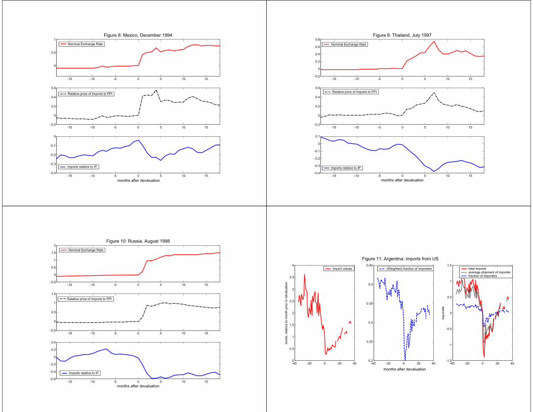
-15 -10 -5 0 5 10 15

0

0.5

1Figure 8: Mexico, December 1994

-15 -10 -5 0 5 10 15-0.2

0

0.2

0.4

0.6

Relative price of Imports to PPI

-15 -10 -5 0 5 10 15-0.4

-0.3

-0.2

-0.1

0

months after devaluation

Nominal Exchange Rate

Imports relative to IP

-15 -10 -5 0 5 10 15-0.2

0

0.2

0.4

0.6

0.8Figure 9: Thailand, July 1997

-15 -10 -5 0 5 10 15-0.2

0

0.2

0.4

0.6Relative price of Imports to PPI

-15 -10 -5 0 5 10 15-0.4

-0.3

-0.2

-0.1

0

0.1

months after devaluation

Imports relative to IP

Nominal Exchange Rate

-15 -10 -5 0 5 10 15-0.5

0

0.5

1

1.5

2Figure 10: Russia, August 1998

-15 -10 -5 0 5 10 15-0.5

0

0.5

1

1.5

-15 -10 -5 0 5 10 15-0.6

-0.4

-0.2

0

0.2

0.4

months after devaluation

Relative price of Imports to PPI

Imports relative to IP

Nominal Exchange Rate

-40 -20 0 20 400

0.5

1

1.5

2

2.5

3

3.5

4

leve

ls, r

elat

ive

to m

onth

prio

r to

deva

luat

ion

Import values

-40 -20 0 20 400.2

0.25

0.3

0.35

0.4

0.45

Figure 11: Argentina: imports from US

months after devaluation-40 -20 0 20 40

-1.5

-1

-0.5

0

0.5

1

1.5

log-

scal

e

total importsaverage shipment of importerfraction of importers

(Weighted) fraction of importers

-40 -20 0 20 400.3

0.4

0.5

0.6

0.7

0.8

0.9

1

1.1

1.2

1.3

leve

ls, r

elat

ive

to m

onth

prio

r to

deva

luat

ion

Import values

-40 -20 0 20 400.35

0.4

0.45

0.5

0.55

months after devaluation

Figure 12: Brazil: Imports from US

-40 -20 0 20 40-1

-0.5

0

0.5

log-

scal

e

total importsaverage shipment of importerfraction of importers

(Weighted) fraction of importers

-40 -20 0 20 40

0.2

0.4

0.6

0.8

1

1.2

1.4

1.6

1.8

leve

ls, r

elat

ive

to m

onth

prio

r to

deva

luat

ion

Import values

-40 -20 0 20 400.35

0.4

0.45

0.5

0.55

0.6

0.65

0.7

Figure 13: Korea: imports from US

months after devaluation-40 -20 0 20 40

-1.2

-1

-0.8

-0.6

-0.4

-0.2

0

0.2

0.4

0.6

log-

scal

e

total importsaverage shipment of importerfraction of importers

(Weighted) fraction of importers

-40 -20 0 20 40

0.5

1

1.5

2

2.5

leve

ls, r

elat

ive

to m

onth

prio

r to

deva

luat

ion

Import values

-40 -20 0 20 400.5

0.55

0.6

0.65

0.7

0.75

0.8

0.85

0.9

Figure 14: Mexico: imports from US

months after devaluation-40 -20 0 20 40

-0.8

-0.6

-0.4

-0.2

0

0.2

0.4

0.6

0.8

1

log-

scal

e

total importsaverage shipment of importerfraction of importers

(Weighted) fraction of importers

-40 -20 0 20 400.2

0.4

0.6

0.8

1

1.2

1.4

1.6

1.8

2

2.2

leve

ls, r

elat

ive

to m

onth

prio

r to

deva

luat

ion

Import values

-40 -20 0 20 400.2

0.25

0.3

0.35

0.4

0.45

0.5

0.55

0.6

0.65

Figure 15: Thailand: imports from US

months after devaluation-40 -20 0 20 40

-1

-0.5

0

0.5

1

log-

scal

e

total importsaverage shipment of importerfraction of importers

(Weighted) fraction of importers

-40 -20 0 20 40

0

0.5

1

1.5

2

leve

ls, r

elat

ive

to m

onth

prio

r to

deva

luat

ion

Import values

-40 -20 0 20 400.05

0.1

0.15

0.2

0.25

0.3

0.35

0.4

0.45

0.5

0.55

Figure 16: Russia: imports from US

months after devaluation-40 -20 0 20 40

-3

-2.5

-2

-1.5

-1

-0.5

0

0.5

1

1.5

log-

scal

e

total importsaverage shipment of importerfraction of importers

(Weighted) fraction of importers

0 1 2 3 4 5 6

1

Figure 17: Ergodic density of inventory holdings and adjustment hazard

0 1 2 3 4 5 6

1

beginning-of-period inventories (relative to mean pre-crisis sales)

adjustment hazard

adjustment hazard

Pre-crisis

Post-crisis

1 1.5 2 2.5 3 3.5 4 4.5 5 5.5 61.2

1.3

1.4

1.5

1.6

1.7

1.8

1.9

2Figure 18: price functions post-crisis

beginning-of-period inventory (relative to mean sales pre-crisis)

rela

tive

to p

rice

of a

djus

ting

firm

in p

re-c

risis

ste

ady-

stat

e

pn(s)

pa(s)

1 1.5 2 2.5 3 3.5 4 4.5 5 5.5 61.2

1.3

1.4

1.5

1.6

1.7

1.8

1.9

2Figure 18: price functions post-crisis

beginning-of-period inventory (relative to mean sales pre-crisis)

rela

tive

to p

rice

of a

djus

ting

firm

in p

re-c

risis

ste

ady-

stat

e

pn(s)

pa(s)

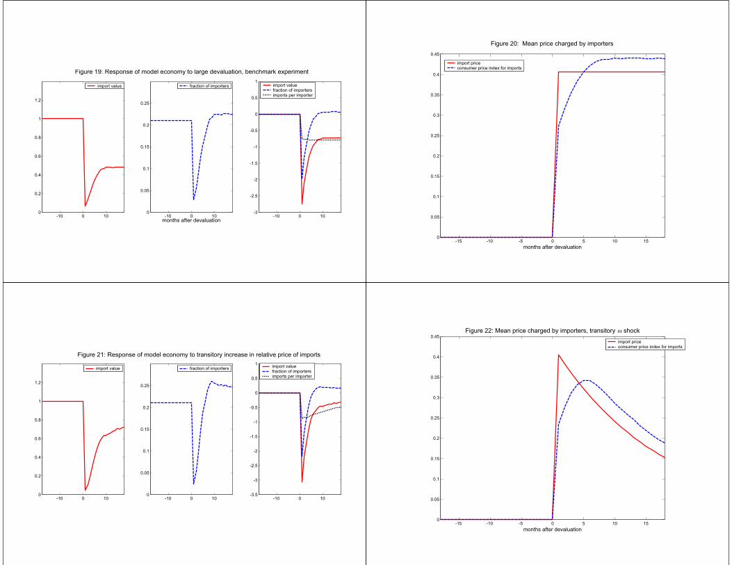
-10 0 100

0.2

0.4

0.6

0.8

1

1.2

-10 0 100

0.05

0.1

0.15

0.2

0.25

months after devaluation

Figure 19: Response of model economy to large devaluation, benchmark experiment

-10 0 10-3

-2.5

-2

-1.5

-1

-0.5

0

0.5

1fraction of importers import value

fraction of importersimports per importer

import value

-15 -10 -5 0 5 10 150

0.05

0.1

0.15

0.2

0.25

0.3

0.35

0.4

0.45

Figure 20: Mean price charged by importers

months after devaluation

import priceconsumer price index for imports

-10 0 100

0.2

0.4

0.6

0.8

1

1.2

import value

-10 0 100

0.05

0.1

0.15

0.2

0.25

Figure 21: Response of model economy to transitory increase in relative price of imports

-10 0 10-3.5

-3

-2.5

-2

-1.5

-1

-0.5

0

0.5

1 import valuefraction of importersimports per importer

fraction of importers

-15 -10 -5 0 5 10 150

0.05

0.1

0.15

0.2

0.25

0.3

0.35

0.4

0.45Figure 22: Mean price charged by importers, transitory shock

months after devaluation

import priceconsumer price index for imports

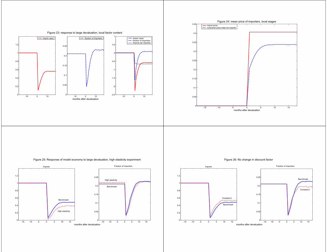
-10 0 100

0.2

0.4

0.6

0.8

1

1.2

import value

-10 0 100

0.05

0.1

0.15

0.2

0.25

Figure 23: response to large devaluation, local factor content

months after devaluation-10 0 10

-2.5

-2

-1.5

-1

-0.5

0

0.5

1import valuefraction of importersimports per importer

fraction of importers

-15 -10 -5 0 5 10 150

0.05

0.1

0.15

0.2

0.25

0.3

0.35

0.4

0.45Figure 24: mean price of importers, local wages

months after devaluation

import priceconsumer price index for imports

-15 -10 -5 0 5 10 150

0.2

0.4

0.6

0.8

1

1.2

Imports

-15 -10 -5 0 5 10 150

0.05

0.1

0.15

0.2

0.25

months after devaluation

Figure 25: Response of model economy to large devaluation, high elasticity experiment

Fraction of importers

Benchmark

High elasticity

High elasticity

Benchmark

-15 -10 -5 0 5 10 150

0.2

0.4

0.6

0.8

1

1.2

Imports

-15 -10 -5 0 5 10 150

0.05

0.1

0.15

0.2

0.25

months after devaluation

Figure 26: No change in discount factor

Fraction of importers

Benchmark

Constant

Benchmark

Constant

-15 -10 -5 0 5 10 150

0.2

0.4

0.6

0.8

1

1.2

Imports

-15 -10 -5 0 5 10 150

0.2

0.4

0.6

0.8

1

1.2

months after devaluation

Figure 27: No fixed cost economy

Fraction of importers

BenchmarkBenchmark

Economy with no fixed costs

Economy with no fixed costs

-15 -10 -5 0 5 10 150

0.2

0.4

0.6

0.8

1

1.2

Imports

-15 -10 -5 0 5 10 150

0.05

0.1

0.15

0.2

0.25

0.3

0.35

months after devaluation

Figure 28: No lag economy

Fraction of importers

Benchmark

BenchmarkNo lag

No lag

-15 -10 -5 0 5 10 150

0.2

0.4

0.6

0.8

1

1.2

Imports

-15 -10 -5 0 5 10 150

0.05

0.1

0.15

0.2

0.25

0.3

0.35

months after devaluation

Figure 28: No lag economy

Fraction of importers

Benchmark

BenchmarkNo lag

No lag