arX

iv:2

108.

0199

1v1

[ee

ss.A

S] 4

Aug

202

11

Lung Sound Classification Using Co-tuning and

Stochastic NormalizationT. Nguyen, and F. Pernkopf, Member, IEEE

Abstract—In this paper, we use pre-trained ResNet modelsas backbone architectures for classification of adventitious lungsounds and respiratory diseases. The knowledge of the pre-trained model is transferred by using vanilla fine-tuning, co-tuning, stochastic normalization and the combination of the co-tuning and stochastic normalization techniques. Furthermore,data augmentation in both time domain and time-frequencydomain is used to account for the class imbalance of the ICBHIand our multi-channel lung sound dataset. Additionally, weapply spectrum correction to consider the variations of therecording device properties on the ICBHI dataset. Empirically,our proposed systems mostly outperform all state-of-the-art lungsound classification systems for the adventitious lung sounds andrespiratory diseases of both datasets.

Index Terms—Adventitious lung sound classification, respi-ratory disease classification, crackles, wheezes, co-tuning fortransfer learning, stochastic normalization, ICBHI dataset.

I. INTRODUCTION

RESPIRATORY diseases have become one of the main

causes of death in society. According to the World Health

Organization (WHO), the ”big five” respiratory diseases,

which include asthma, chronic obstructive pulmonary disease

(COPD), acute lower respiratory tract infections, lung cancer

and tuberculosis, cause the mortality of more than 3 million

people each year worldwide. Currently, CoViD-19, a special

form of viral pneumonia related to the coronavirus identified

firstly in Wuhan (China) in 2019 [1], has caused globally

more than 158 million infections and 3,296,000 deaths [2]. On

March 11, 2020, the WHO officially announced that CoViD-19

has reached global pandemic status. Furthermore, according

to [3], the “big five” lung diseases, except lung cancer,

have increased during CoViD-19 epidemics. These respiratory

diseases are characterised by highly similar symptoms, i.e.

the adventitious breathing, which could be a confounding

factor during diagnosis [1]. Due to their severe consequences,

particularly in the case of CoViD-19, an early and accurate

diagnosis of these types of diseases has become crucial.

Lung sounds convey relevant information related to pul-

monary disorders with adventitious breathing sounds such as

crackles, wheezes, or both of crackles and wheezes [4], [5]. In

the last decades, to facilitate a more objective assessment of

the lung sound for diagnosis of pulmonary diseases/conditions,

computational methods i.e. computational lung sound analysis

Thanks to the Vietnamese - Austrian Government scholarship and theAustrian Science Fund (FWF) under the project number I2706-N31.

T. Nguyen, is with Signal Processing and Speech Communication Lab. GrazUniversity of Technology, Austria (e-mail: t.k.nguyen@tugraz.at).

F. Pernkopf is with Signal Processing and Speech Communication Lab.Graz University of Technology, Austria (e-mail: pernkopf@tugraz.at).

(CLSA) [6], [7] have been developed. The CLSA systems

automatically detect and classify adventitious lung sounds by

using digital recording devices, signal processing techniques

and machine learning algorithms. They are also carefully

evaluated in real-life scenarios and can be used as portable

easy-to-use devices without the necessity of expert interac-

tion; especially, beneficial when facing infectious diseases as

CoViD-19.

In CLSA systems, there are two popular classification

tasks, namely (i) adventitious lung sound and (ii) respiratory

disease classification. In adventitious lung sound classifica-

tion, recognition of normal and abnormal sounds (i.e. either

crackles or wheezes or both of them) is important; while for

respiratory disease classification, several categories have been

considered e.g. binary classification (health and pathological),

ternary chronic classification (healthy, chronic and non-chronic

diseases) or six class classification of distinct pathologies. The

systems have been evaluated on non-public datasets such as

R.A.L.E. [8] or multi channel lung sound data [9] (ours) and

public datasets i.e. the ICBHI 2017 dataset [5] or the Abdullah

University Hospital 2020 dataset [10]. Due to limitations in

the amount and quality of available data, the performance and

generalization of the lung sound classification system may

suffer over-estimated results. To deal with these challenges,

different feature extraction methods [11], [12], [13], [14],

conventional machine learning [12], [15], [16], [17], [18], deep

learning [19], [20], [21], [22], data augmentation and transfer

learning from ImageNet [23], [24], or audio scene datasets [25]

have been explored.

In this work, we improve the generalization ability and

model performance for adventitious lung sound classification

and respiratory disease classification systems using the ICBHI

2017 dataset and our multi-channel lung sound dataset. We

exploit transfer learning approaches such as co-tuning [26] for

different architectures of residual neural networks (ResNets).

We use pre-trained ResNet models of the ImageNet classifica-

tion task as backbone architectures, which requires a 3-channel

input i.e. color RGB images. Therefore the spectrograms are

converted into 3 channels for the model input. Particularly,

logmel spectrograms are replicated into three channels for the

adventitious lung sound task or converted into RGB color

spectrogram for respiratory disease classification. The pre-

trained models are exploited systematically in the following

compositions.

• Firstly, we fine-tune the pre-trained model on a target

domain and update all top (i.e. feature representation)

layers and bottom (i.e. task-specific) layers. We call this

vanilla fine-tuning.

2

• Secondly, we apply co-tuning for transfer learning [26],

in which representation layers and task-specific layers of

both source domain and target domain are collaboratively

fine-tuned. Co-tuning further updates task-specific layers

of the pre-trained model using a learned category rela-

tionship between source and target domains.

• Thirdly, we replace Batch Normalization (BN) layers,

which suffer from poor performance in case of a data

distribution shift between training and test data. We

introduce stochastic normalization (StochNorm) [27] in

each residual block of the pre-trained backbone architec-

ture. StochNorm is a parallel structure normalizing the

activation of each channel by either mini-batch statistics

or moving statistics to avoid influence of sample statistics

during training. Thus, it is considered as a regularization

method. Furthermore, fine-tuning inherits further prior

knowledge of moving statistics of the pre-trained net-

works compared to vanilla fine-tuning. Both properties

help to avoid over-fitting on small datasets such as the

ICBHI and our lung sound dataset.

• Finally, we combine co-tuning and stochastic normaliza-

tion techniques to take advantages of both techniques.

In addition, we apply data augmentation in both time domain

and time-frequency domain to account for the class imbalance

in the datasets. Furthermore, we use spectrum correction for

lung sound classification to compensate the recording device

variations in the ICBHI dataset. The main contributions of the

paper are:

• We propose robust classification systems for adventitious

lung sounds and respiratory diseases for the ICBHI and

our multi-channel lung sound dataset.

• We exploit transferred knowledge of pre-trained models

by vanilla fine-tuning, co-tuning, stochastic normalization

techniques and a combination of both co-tuning and

stochastic normalization.

• We introduce spectrum correction to improve the gener-

alization ability by accounting for the recording device

differences.

• In addition to commonly used data augmentation tech-

niques, we double the size of the training dataset by

flipping samples in target domain. This enhances the

performance of adventitious lung sound classification.

• We review state-of-the-art adventitious lung sound and

respiratory disease classification systems for the ICBHI

and our multi-channel lung sound dataset.

The outline of the paper is as follows: In Section II,

we introduce the lung sound databases. In Section III, we

present our lung sound classification systems. In Section IV,

we present the experimental setup including the evaluation

metrics and the experimental results. We review related works

in Section V. Finally, we conclude the paper in Section VI.

II. DATABASES

A. ICBHI 2017 Dataset

The ICBHI 2017 database [5] consists of 920 annotated

audio samples from 126 subjects corresponding to patient

pathological conditions i.e. healthy and seven distinct disease

categories (Pneumonia, Bronchiectasis, COPD, upper respira-

tory tract infection (URTI), lower respiratory tract infection

(LRTI), Bronchiolitis, Asthma). The audios were recorded us-

ing different stethoscopes i.e. AKGC417L, Meditron, Litt3200

and LittC2SE. The recording duration ranges from 10s to 90s

and the sampling rate ranges from 4000Hz to 44100Hz. Each

recording is composed of a certain number of breathing cycles

with corresponding annotations of the beginning and the end,

and the presence/absence of crackles and/or wheezes. The

annotations of the database supports to split audio recordings

into respiratory cycles. The cycle duration ranges from 0.2s

to 16s and the average cycle duration is 2.7s. The database

includes 6898 different respiratory cycles with 3642 normal

cycles, 1864 crackles, 886 wheezes, and 506 cycles containing

of both crackles and wheezes.

We propose a classification system for the following tasks.

• ALSC: Adventitious lung sound classification (ALSC) is

separated into two sub-tasks for respiratory cycles. The

first one is a 4-class task classifying respiratory cycles

into four classes (Normal, Crackles, Wheezes and both

Crackles and Wheezes). The second sub-tasks is a 2-

class task of normal and abnormal lung sounds including

Crackles, Wheezes and both Crackles and Wheezes. We

evaluate our system on the official ICBHI data split. The

dataset was divided by the ICBHI challenge into 60%

for training and 40% for testing. Both sets are composed

with different patients.

• RDC: Respiratory disease classification (RDC) also con-

sists of two sub-tasks for audio recordings. The first

one is a 3-class task classifying audio recordings into

three groups of Healthy, Chronic Diseases (i.e. COPD,

Bronchiectasis and Asthma) and Non-Chronic Diseases

(i.e. URTI, LRTI, Pneumonia and Bronchiolitis). The sec-

ond sub-tasks is a 2-class task (healthy/unhealthy), where

the unhealthy class comprises of the seven diseases.

B. Multi-channel Lung Sound Database

The multi-channel lung sound database [9], [19], [28] has

been recorded in a clinical trial. It contains lung sounds of

16 healthy subjects and 7 patients diagnosed with idiopathic

pulmonary fibrosis (IPF). We used our 16-channel lung sound

recording device (see Fig. 1) to record lung sounds over

the posterior chest at two different airflow rates, with 3

- 8 respiratory cycles within 30s. The lung sounds were

recorded with a sampling frequency of 16kHz. The sensor

signals are filtered with a Bessel high-pass filter with a cut-off

frequency of 80Hz and a slope of 24dB/oct. We extracted full

respiratory cycles using the airflow signal from all recordings.

We manually annotated respiratory cycles in cooperation with

respiratory experts from Medical University of Graz, Austria.

The number of breathing cycles with/without IPF are shown

in Table I.

III. TRANSFER LEARNING FOR LUNG SOUND

CLASSIFICATION

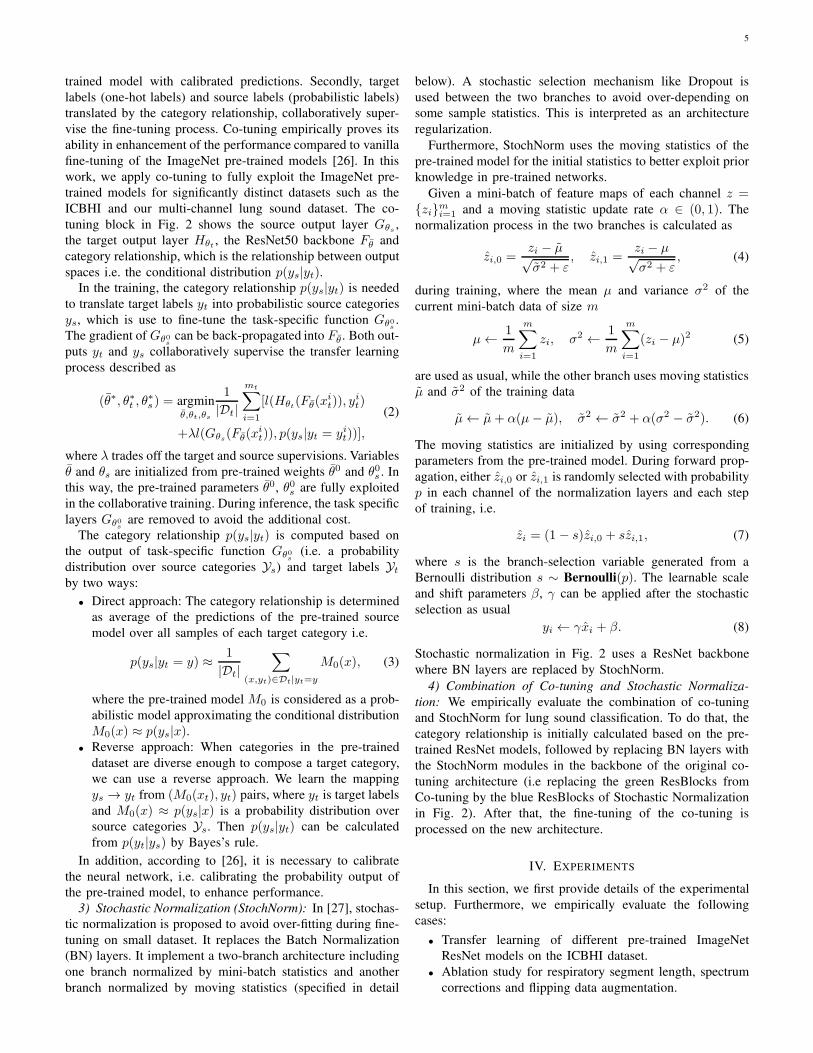
The proposed systems include two key stages i.e. feature

processing and classification as shown in Fig. 2. Firstly,

3

Fig. 1. Multi-channel lung sound recording device.

TABLE INUMBER OF SUBJECTS AND CYCLES IN THE DATASET

# Subjects # Respiratory Cycles

Healthy IPF Normal Crackles Total

16 7 4405 1791 6196

the respiratory cycles/ recordings are pre-processed in time

domain and transformed into log-mel spectrograms of fixed

size. Secondly, the features are fed to the CNN model where

co-tuning or stochastic normalization are explored for the

different classification tasks. During inference, the label of an

input respiratory cycle/ recording is determined via majority

voting [29] of the predicted labels of the individual segments

with a length of 8 seconds belonging to the same recording.

A. Audio Pre-processing and Feature Extraction

We use the audio pre-processing and feature extraction tech-

niques presented in [22] for both datasets. Audio recordings

are resampled to 16kHz for the ALSC tasks of the ICBHI

challenge and our dataset, while the RDC tasks use 4kHz of

sampling rate. Similar to our previous works on ALSC of

ICBHI and our multi-channel dataset [22], [30], the respiratory

cycles are split without overlap into segments. Furthermore,

we apply sample padding in time-reversed order to achieve

fixed-length segments without abrupt signal changes. For the

RDC task of the ICBHI dataset, recordings are split into

segments of the same length using 50% overlap. Different

segment lengths are investigated in Section IV. Then we also

applied sample padding to the segments being shorter than the

fixed length. This means that for both respiratory cycles and

recordings, the same splitting and sample padding procedure

is applied to obtain the fixed-length segments for the ALSC

and RDC tasks, respectively.

We use a window size of 512 samples for the fast Fourier

transform (FFT) using 50% overlap between the windows. The

number of mel frequency bins is chosen as 50 and 45 for

the ICBHI dataset and our multi-channel dataset, respectively.

The logarithmic scale is applied to the magnitude of the mel

spectrograms. The log-mel spectrograms are normalized with

zero mean and unit variance. Then these spectrograms are

duplicated into three channels to match the input size of the

pre-trained ResNet model for the ALSC task. However, for the

RDC task of the ICBHI dataset, we convert the spectrogram

into a RGB color image and enlarge the image to twice the

size using linear interpolation.

TABLE IIPERCENTAGE OF SAMPLES RECORDED BY EACH DEVICE OF THE ICBHI

DATASET

Device AKGC417L Meditron Litt3200 LittC2SE

% Sample 63% 21% 9% 7%

B. Spectrum Correction

We observe a different frequency response across de-

vices which results in a performance degradation for under-

represented devices. Hence, we calibrate the features of the au-

dio segments by applying spectrum correction instead of train-

ing or fine-tuning the model for a specific device [31], [32].

The spectrum correction or calibration proposed in [33], which

was first applied for acoustic scene classification, scales the

frequency response of the recording devices. In particular, the

calibration coefficients are calculated for each device based

on data from reference devices. Table II shows the recorded

data portions of each recording device of the ICBHI dataset.

The magnitude spectrum ski of each segment i recorded by the

device k is an averaged spectrum along the time axis of all

FFT windows. The mean device spectrum sk = 1Nk

∑Nk

i=1 ski ,

where device k records Nk segments corresponding to Nk

spectra. The reference spectrum sref is furthermore averaged

over all mean device spectra of the D reference devices

sref = 1|D|

∑k∈D sk, where D contains the indices of the

reference devices. We investigate different cases of reference

devices based on their prominence i.e only one device either

AKGC417L or Meditron or both AKGC417L and Meditron,

or all recording devices. The scaling coefficients of each

device (ck) is the element-wise fraction (i.e for each frequency

bin) of the reference spectrum and its corresponding device

spectrum ck =sref

sk. The magnitude of the STFTs of each

device is scaled by using the corresponding coefficient vector

ck for the frequency bins. We empirically observed that the

normalization in spectrogram domain is more successful than

in log-mel domain.

C. Data Augmentation

The ICBHI 2017 dataset is extremely imbalanced with

around 53% of respiratory cycles belonging to the normal class

and 86% of audio recordings belonging to COPD. Further-

more, with our multi-channel lung sound dataset, around 71%

of respiratory cycles are annotated as normal class. Therefore,

we use data augmentation in both time domain and time -

frequency domain in order to balance the training dataset and

prevent over-fitting.

1) Time Domain: For ALSC of the ICBHI dataset, we

use time stretching to increase/reduce the sampling rate of

an audio signal without affecting its pitch [34]. It is used

to double the number of segments of the wheeze, and both

wheeze and crackle classes. We use a random sampling rate

uniformly distributed with ±10% of the original sampling rate.

For RDC of ICBHI, time stretching is used for all classes to

double the number of samples. Furthermore, on the doubled

training set further data augmentation methods1 i.e volume

1https://github.com/makcedward/nlpaug

4

Lung sound

Sample

Padding

8s

STFT

8s

Spectrum

Correction

Log-Mel &

Normalization

Re

sNe

t50

Ba

ckb

on

e

So

urc

e

Ou

tpu

t La

ye

r

Targ

et

Ou

tpu

t La

ye

r

Ca

teg

ory

Re

lati

on

ship

Avg Pooling

ResBlock

…

ResBlock

Conv2D,7x7, 64

Target

Output Layer

Avg Pooling

ResBlock

…

ResBlock

Conv2D,7x7, 64

Co-tuning for Transfer Learning Stochastic Normalization

4-class

Feature Processing

3-class 2-class 4-class 3-class 2-class

H�t

G�s

F�

Re

sNe

t50

Ba

ckb

on

e

Fig. 2. Proposed transferred knowledge systems using co-tuning for transfer learning or stochastic normalization.

adjusting, noise addition, pitch adjusting and speed adjusting

are randomly applied based on a predefined probability.

2) Time-Frequency Domain:

• Vocal tract length perturbation (VTLP) selects a random

wrap factor α for each recording and maps the frequency

f of the signal bandwidth to a new frequency f ′ [35].

We select α from a uniform distribution α ∼ U(0.9, 1.1)and set the maximum signal bandwidth to Fhi = [3200,

3800]. VTLP is applied directly to the mel filter bank

rather than distorting each spectrogram. VTLP is applied

to enlarge the dataset for all classes in both tasks for both

the original training set and the time stretched data.

• Additionally, we double the log-mel features by adding

the flipped log-mel features (in frequency axis) for the

ALSC and crackle detection task of our dataset.

D. Exploiting Transferred Knowledge

1) Transfer Learning: Deep neural networks (DNNs)

trained from scratch require large amounts of data. As data

collecting is a time consuming task for lung sound data,

transferring pre-trained parameters from DNNs, which are

trained on other datasets e.g. ImageNet is advantageous. Less

data of the target task is required, faster training is enabled,

and usually better performance after fine-tuning the model on

the target task is achieved [36]. Therefore, fine-tuning brings

great benefit to the research community.

Given a DNN M0 pre-trained on a source dataset Ds ={(xi

s, yis)}ms

i=1, transfer learning aims to fine-tune M0 on a

target dataset Dt = {(xit, y

it)}mt

i=1. In this work, Ds is selected

from ImageNet and Dt is the ICBHI 2017 dataset or our

multi-channel lung sound dataset. Only Dt and the pre-trained

model M0 are available during fine-tuning. Because Ds and Dt

are different domains, which may have different input spaces

Xs and Xt, corresponding to different output spaces Ys and

Yt, respectively. Therefore, M0 can not be directly applied

to the target data. It is common practice, to split M0 into

two parts: a general representation function Fθ0 (parametrized

by θ0) and a task-specific function Gθ0s

(parametrized by θ0s ),

which denotes the last layers of the pre-trained model. Usually,

the representation function is retained and the task-specific

function is replaced by a randomly initialized function Hθt

(parameterized by θt) whose output space matches Yt. Hence,

we optimize

(θ∗, θ∗t ) = argminθ,θt

1

|Dt|

mt∑

i=1

l(Hθt(Fθ(xit)), y

it), (1)

where l(·) is a loss function such as cross-entropy for classi-

fication. We will call this vanilla fine-tuning. Pre-trained pa-

rameters θ0 provide a good starting point for the optimization.

It means that the vanilla fine-tuning for a target dataset can

be beneficial by transferring the knowledge of the part Fθ0 of

the source dataset.

In this work, we explore different depths of ResNet archi-

tectures i.e. ResNet18, ResNet34, ResNet50 and ResNet101

as neural network backbones.

2) Co-tuning: Co-tuning for transfer learning enables full

knowledge transfer of the pre-trained models using a two-

step framework [26]. The first step is learning the relationship

between source categories and target categories from the pre-

5

trained model with calibrated predictions. Secondly, target

labels (one-hot labels) and source labels (probabilistic labels)

translated by the category relationship, collaboratively super-

vise the fine-tuning process. Co-tuning empirically proves its

ability in enhancement of the performance compared to vanilla

fine-tuning of the ImageNet pre-trained models [26]. In this

work, we apply co-tuning to fully exploit the ImageNet pre-

trained models for significantly distinct datasets such as the

ICBHI and our multi-channel lung sound dataset. The co-

tuning block in Fig. 2 shows the source output layer Gθs ,

the target output layer Hθt , the ResNet50 backbone Fθ and

category relationship, which is the relationship between output

spaces i.e. the conditional distribution p(ys|yt).In the training, the category relationship p(ys|yt) is needed

to translate target labels yt into probabilistic source categories

ys, which is use to fine-tune the task-specific function Gθ0s.

The gradient of Gθ0s

can be back-propagated into Fθ . Both out-

puts yt and ys collaboratively supervise the transfer learning

process described as

(θ∗, θ∗t , θ∗s ) = argmin

θ,θt,θs

1

|Dt|

mt∑

i=1

[l(Hθt(Fθ(xit)), y

it)

+λl(Gθs(Fθ(xit)), p(ys|yt = yit))],

(2)

where λ trades off the target and source supervisions. Variables

θ and θs are initialized from pre-trained weights θ0 and θ0s . In

this way, the pre-trained parameters θ0, θ0s are fully exploited

in the collaborative training. During inference, the task specific

layers Gθ0s

are removed to avoid the additional cost.

The category relationship p(ys|yt) is computed based on

the output of task-specific function Gθ0s

(i.e. a probability

distribution over source categories Ys) and target labels Ytby two ways:

• Direct approach: The category relationship is determined

as average of the predictions of the pre-trained source

model over all samples of each target category i.e.

p(ys|yt = y) ≈ 1

|Dt|∑

(x,yt)∈Dt|yt=y

M0(x), (3)

where the pre-trained model M0 is considered as a prob-

abilistic model approximating the conditional distribution

M0(x) ≈ p(ys|x).• Reverse approach: When categories in the pre-trained

dataset are diverse enough to compose a target category,

we can use a reverse approach. We learn the mapping

ys → yt from (M0(xt), yt) pairs, where yt is target labels

and M0(x) ≈ p(ys|x) is a probability distribution over

source categories Ys. Then p(ys|yt) can be calculated

from p(yt|ys) by Bayes’s rule.

In addition, according to [26], it is necessary to calibrate

the neural network, i.e. calibrating the probability output of

the pre-trained model, to enhance performance.

3) Stochastic Normalization (StochNorm): In [27], stochas-

tic normalization is proposed to avoid over-fitting during fine-

tuning on small dataset. It replaces the Batch Normalization

(BN) layers. It implement a two-branch architecture including

one branch normalized by mini-batch statistics and another

branch normalized by moving statistics (specified in detail

below). A stochastic selection mechanism like Dropout is

used between the two branches to avoid over-depending on

some sample statistics. This is interpreted as an architecture

regularization.

Furthermore, StochNorm uses the moving statistics of the

pre-trained model for the initial statistics to better exploit prior

knowledge in pre-trained networks.

Given a mini-batch of feature maps of each channel z ={zi}mi=1 and a moving statistic update rate α ∈ (0, 1). The

normalization process in the two branches is calculated as

zi,0 =zi − µ√σ2 + ε

, zi,1 =zi − µ√σ2 + ε

, (4)

during training, where the mean µ and variance σ2 of the

current mini-batch data of size m

µ← 1

m

m∑

i=1

zi, σ2 ← 1

m

m∑

i=1

(zi − µ)2 (5)

are used as usual, while the other branch uses moving statistics

µ and σ2 of the training data

µ← µ+ α(µ− µ), σ2 ← σ2 + α(σ2 − σ2). (6)

The moving statistics are initialized by using corresponding

parameters from the pre-trained model. During forward prop-

agation, either zi,0 or zi,1 is randomly selected with probability

p in each channel of the normalization layers and each step

of training, i.e.

zi = (1 − s)zi,0 + szi,1, (7)

where s is the branch-selection variable generated from a

Bernoulli distribution s ∼ Bernoulli(p). The learnable scale

and shift parameters β, γ can be applied after the stochastic

selection as usual

yi ← γxi + β. (8)

Stochastic normalization in Fig. 2 uses a ResNet backbone

where BN layers are replaced by StochNorm.

4) Combination of Co-tuning and Stochastic Normaliza-

tion: We empirically evaluate the combination of co-tuning

and StochNorm for lung sound classification. To do that, the

category relationship is initially calculated based on the pre-

trained ResNet models, followed by replacing BN layers with

the StochNorm modules in the backbone of the original co-

tuning architecture (i.e replacing the green ResBlocks from

Co-tuning by the blue ResBlocks of Stochastic Normalization

in Fig. 2). After that, the fine-tuning of the co-tuning is

processed on the new architecture.

IV. EXPERIMENTS

In this section, we first provide details of the experimental

setup. Furthermore, we empirically evaluate the following

cases:

• Transfer learning of different pre-trained ImageNet

ResNet models on the ICBHI dataset.

• Ablation study for respiratory segment length, spectrum

corrections and flipping data augmentation.

6

• Transfer learning of different ResNet models pre-trained

on ImageNet and ICBHI for our multi-channel lung sound

dataset.

Our systems for the ALSC and RDC tasks on the ICBHI

dataset are also compared against state-of-the-art works for

the official ICBHI data split and five-fold cross-validation.

Additionally, we compare our best system for crackle detection

to our previous work on the multi-channel lung sound dataset.

A. Evaluation Metrics

We use the evaluation metrics supported by the ICBHI

Challenge [5] for ALSC of 4 classes. The evaluation is based

on respiratory cycles using sensitivity (SE), specificity (SP),

average score (AS), known as the average of the sensitivity

and the specificity, and the harmonic score (HS), known as

the harmonic mean of the sensitivity and the specificity. For 2

classes, we determine SE and SP as in [20] and [14] and AS

and HS as in [5].

Similarly, for RDC of 3 classes and 2 classes, a recording-

wise evaluation is performed using SE and SP as in [20]

and [14] and AS and HS as in [5].

Furthermore, for our multi-channel lung sound dataset, we

calculate Precision (P+), Sensitivity or Recall (Se), and the

F1-score (F1) as specified in [19]. Precision provides infor-

mation about how many of the respiratory cycles recognized

as crackles are actually true. Sensitivity provides information

about how many respiratory cycles containing crackles are

actually recognized as crackles. The F1-score is the harmonic

mean of precision and sensitivity.

B. Experimental Setup

We evaluate our ALSC system for 4 and 2 classes on

the official ICBHI 2017 dataset split, which consists of 60%

recordings for the training set and 40% for the test set. Each

patients is either in the training or test set. The reported

performance is the average accuracy of five independent runs.

For the RDC task of 3 and 2 classes, our proposed system is

evaluated on both the official dataset split and five-fold cross-

validation. Again, data of each patients is not shared between

folds. For five-fold cross-validation, one fold is used as test

set, the remaining folds are used for training. As co-tuning

requires a validation set to compute the category relationship,

we randomly select 20% of the samples from the training set.

For cross-validation, the average of the best performance on

the test sets is represented.

Due to the limited amount of data samples in our multi-

channel lung sound dataset, we use 7-fold cross-validation

with the recordings of each IPF subject appearing once in the

test set. Each subject is assigned to either training, validation

or test set. The best model is selected based on the best

accuracy on the validation set. The reported performance of

the system is an average accuracy of seven folds using the

same data splittings.

Experiments are implemented based on Pytorch [37]. For

vanilla fine-tuning, the learning rate and number of epochs is

set to 0.001 and 150 for all tests, respectively. The fine-tuning

of co-tuning and stochastic normalization techniques2 updates

the weights after each mini-batch. The learning rate of the

feature representation layers and the last layer are set to 0.001

and 0.01, respectively. The fine-tuning process optimizes the

cross entropy loss using SGD with a momentum of 0.9. The

batch size is 32 for all experiments.

C. Experimental Results

1) Transfer learning techniques for different ResNets:

We evaluate the vanilla fine-tuning (VanillaFineTuning), co-

tuning (CoTuning), stochastic normalization (StochNorm) and

the combination of co-tuning and stochastic normaliza-

tion (CoTuning-StochNorm) for different ResNet architectures

trained on the ImageNet dataset for the ALSC task of 4 classes

(see Fig. 3) and the RDC task of 3 classes (see Fig. 5) on

the official ICBHI dataset split. These systems use a segment

length of 8s, spectrum correction using reference data sref of

all devices and all data augmentation methods introduced in

Section C.

Fig. 3 shows that ResNet50 is the best performing archi-

tecture to build the backbone for these transfer learning tech-

niques of the 4-class ALSC task. ResNet101 is also performing

well except for vanilla fine-tuning. Co-tuning achieved the

best performance of ∼58% compared to the other techniques.

Although CoTuning and StochNorm improve significantly the

performance of VanillaFineTuning, the combination of co-

tuning and StochNorm is not able to outperform the original

techniques for this task.

Fig. 4 visualizes of the average pooling outputs of the

ResNet50 architecture for different transfer learning tech-

niques projected to 2D by t-distributed stochastic neighbour-

hood embedding (t-SNE) [38]. Distributions of the training set

using vanilla fine-tuning, co-tuning, stochastic normalization

and combination of co-tuning and stochastic normalization

are shown at a), b), c) and d), respectively. Comparing to

vanilla fine-tuning (a) and stochastic normalization technique

(c), the distribution of 4 classes using co-tuning (b) and the

combination of co-tuning and stochastic normalization (d)

bring a large margin. It shows that the collaborative fine-tuning

using the category relationship of source and target domain is

useful for the adventitious lung sound classification task.

In Fig. 5, we see that the different transfer learning tech-

niques using the ResNet101 model achieve the best per-

formance for the 3-class RDC task. The ResNet50 model

works better than others for the vanilla fine-tuning. CoTuning-

StochNorm and StochNorm achieved a better performance

compared to CoTuning and VanillaFineTuning. It proves the

efficiency of the stochastic normalization in the fine-tuning

process for the RDC task.

2) Respiratory segment length: The length of respiratory

cycles in the ICBHI dataset varies in a wide range. Hence,

we applied cycle splitting into segments and perform sample

padding in order to obtain fixed-length segments. We observe

different segment lengths for the ResNet 50 model fine-tuned

by co-tuning and applied data augmentation in both time

2Code are available at https://github.com/thuml/Cotuning andhttps://github.com/thuml/StochNorm.

7

Fig. 3. Comparison of vanilla transfer learning, co-tuning, stochastic normal-ization and both co-tuning and stochastic normalization of different ResNetbackbones for the adventitious lung sound classification task of 4 classes.

a) b)

c) d)

Fig. 4. Average pooling output representations reduced into 2D by t-distributed stochastic neighborhood embedding (t-SNE) of the ResNet50backbone architecture. Distributions of training set of a) vanilla fine-tuning,b) co-tuning, c) stochastic normalization d) combination of co-tuning andstochastic normalization. The color indicates the classes.

domain and time-frequency domain with spectrum correction.

Results are shown in Table 3. The best score is obtained with

8s fixed-length segments (AS) for 4 classes. We also use 8s

as the fixed length for other tasks of the ICBHI and our lung

sound dataset.

3) Spectrum correction: We experiment on the ICBHI

dataset without spectrum calibration and with spectrum cal-

ibration using different reference spectra sref , which are

determined by one or more devices. No-Calib denotes that

no spectrum correction is applied. Calib-Dev1 and Calib-

Dev2 denote calibration using data of device AKGC417L and

Meditron, respectively. Calib-Dev1Dev2 denotes calibration

using data of both devices of AKGC417L and Meditron and

Calib-AllDev denotes spectrum adaptation using reference data

of four devices. From Table IV, we can see that co-tuning

of the ResNet50 model using reference data of all devices

achieves the best performance, it is 1.62% (absolute) better

than without using spectrum calibration. Thus, we apply spec-

trum calibration for both adventitious lung sound classification

and respiratory diseases classification.

4) Flipping data augmentation: We apply data augmenta-

tion in time domain and VTLP in order to balance the dataset.

Fig. 5. Comparison of vanilla transfer learning, co-tuning, stochastic normal-ization and both co-tuning and stochastic normalization of different ResNetbackbones for the respiratory disease classification task of 3 classes.

TABLE IIIRESPIRATORY SEGMENT LENGTH: AVERAGE SCORE (AS) FOR VARIOUS

INPUT LENGTH SIZES USING CO-TUNING OF RESNET50 AS BACKBONE

NETWORK AND DATA AUGMENTATION WITHOUT SPECTRUM

CALIBRATION.

Length. 4 sec 5 sec 6 sec 7 sec 8 sec 9 sec

AS 54.22 56.25 56.13 56.55 56.67 56.58

± 2.27 ± 1.71 ± 1.17 ± 0.91 ± 1.16 ± 1.03

In this section we focus on the influence of feature flipping

data augmentation (see Section III). Fig. 6 shows that when

the system does not use spectrum correction, doubling the size

of the augmented training set by the flipping technique always

performs well for vanilla fine-tuning, co-tuning and stochastic

normalization. It improves significantly the performance of

vanilla fine-tuning and stochastic normalization of about 3%

and 2%, respectively. For co-tuning, the flipping data augmen-

tation achieves an improvement of 1% accuracy. Furthermore,

we can see from Fig. 6 that using the combination of spectrum

calibration and flipping data augmentation always enhances

the robustness of the adventitious lung sound classification

systems.

5) Effect of pre-trained model on the multi-channel lung

sound dataset: According to the above evaluation of transfer

learning techniques for different residual neural networks

for the 4-class ALSC task, co-tuning achieves the best

performance. Thus, we evaluate the effect of pre-trained

models using co-tuning (CoTuning) for the 2-class ALSC

task on our multi-channel lung sound dataset. It is shown

in Fig. 7. Co-tuning using the ImageNet pre-trained model

always outperforms that of the ICBHI pre-trained model. The

smaller ResNet architectures tend to work better for co-tuning.

We also can see from Fig. 7 that the ResNet34 backbone

system achieves the best performance, followed by ResNet18,

ResNet50 and ResNet101. In addition, Fig. 7 shows that

transferred knowledge from full pre-trained models of ICBHI

and the ImageNet dataset by co-tuning to our small lung sound

dataset can achieve better accuracy than vanilla fine-tuning

(VanillaFineTuning) using the ImageNet pre-trained model.

Overall, the best segment length for lung sound classifi-

cation tasks is 8s. Spectrum correction is useful to improve

8

TABLE IVCOMPARISON OF SPECTRUM CORRECTION METHODS USING DIFFERENT

REFERENCE DATA. CO-TUNING OF THE RESNET50 WITH DATA

AUGMENTATION IS USED.

No-Calib Calib-Dev1 Calib-Dev2 Calib-Dev1Dev2 Calib-AllDev

AS 56.67 57.85 57.85 57.34 58.29

± 1.16 ± 0.40 ± 1.00 ± 0.26 ± 0.46

Fig. 6. Comparison of vanilla transfer learning, co-tuning and stochasticnormalization using ResNet50 for the cases of spectrum correction andflipping data augmentation.

the performance of our ALSC and RDC system on the

ICBHI dataset. This helps to correct the different frequency

responses of the recording devices. The ALSC system using

the flipping data augmentation enhances performance on both

ICBHI and our multi-channel lung sound dataset. The new

transfer learning methods always outperform vanilla transfer

learning. Co-tuning works better for the ALSC task while

StochNorm and its combination with the co-tuning achieve

higher performance for the RDC task. Furthermore, ResNet34

and ResNet50 are more suitable for the ALSC tasks, while a

large ResNet101 model tends to be more robust for the RDC

task in most of transfer learning settings.

D. Performance Comparison

1) Comparison to state-of-the-art systems using the ICBHI

dataset: Table VI and Table VII show the comparison of

our best systems of different transfer learning techniques and

state-of-the-art systems (see Section V for more details on

the systems) for the ALSC and RDC tasks, respectively. Our

best systems are presented in bold and the highest scores

are presented in bold and italic. It is notable that the per-

formances on the official 60/40 ICBHI separation without

common patients in both sets are significantly lower than

that of randomly 80/20 splitting i.e. 5-fold cross validation

and overlap of the same patients in both sets. Despite of the

same fixed length for segments, the RDC systems always

achieve considerably higher performance compared to the

ALSC system for different sub-tasks. The RDC tasks have

the full audio recordings which consists of many available

respiratory cycles, while the ALSC tasks are processed and

evaluated on respiratory cycles.

We evaluate our proposed system on the official ICBHI

split for the 4 and 2 class ALSC tasks. Our best systems of

Fig. 7. Comparison of co-tuning and vanilla fine-tuning of different ResNetarchitectures pre-trained on ICBHI and ImageNet for crakle detection. Ourmulti-channel lung sound dataset and flipping data augmentation are used.

TABLE VCOMPARISON BETWEEN THE PROPOSED SYSTEMS AND THE SYSTEM

IN [30] USING OUR MULTI-CHANNEL LUNG SOUND DATASET FOR

CRACKLE DETECTION TASK

Method Se(%) P+(%) F1-Score(%)

MI-CNN, ICBHI FineTuning [30] 85.32 84.11 84.77

ResNet34, ICBHI CoTuning (Ours) 81.42 94.70 86.81

ResNet34, ImageNet CoTuning (Ours) 82.17 95.88 87.59

ResNet50, ImageNet StochNorm (Ours) 81.82 95.22 87.42

ResNet50, ImageNet CoTuning-StochNorm (Ours) 80.84 94.90 86.46

ResNet50, ImageNet VanillaFineTuning (Ours) 77.42 96.59 85.39

different fine-tuning techniques outperform the other ALSC

systems. Our system using co-tuning of the ResNet50 pre-

trained model achieve the highest ICBHI average score at

58.29% and 64.74% for the 4-class and 2-class ALSC task,

respectively. Our RDC systems are evaluated on the official

ICBHI split and the 5-fold cross-validation method. On the

official dataset split of the 3-class RDC task, our systems

achieves the best performance with the ResNet101 pre-trained

architecture combined with stochastic normalization. It obtains

92.72% of the ICBHI average score. While for the 5-fold

cross-validation evaluation, the stochastic normalization of the

ResNet101 model obtains the best average score 95.73%. It

has an around 5% better average score compared to the state-

of-the-art systems. On the 2-class RDC task, our systems

using stochastic normalization achieves the average scores

of 93.77% and 98.20% for the official splitting and 5-fold

cross-validation, respectively. Our best 2-class RDC system

outperforms all compared systems on the former evaluation,

but it scores 1.02% lower compared to the system in [39].

2) Comparison for our multi-channel lung sound dataset:

Table V compares our best systems using different transfer

learning techniques with our previous system using fine-tuning

for a multi-input CNN model [30] on the multi-channel lung

sound dataset. We can see that our best transfer learning

systems outperform the previous system. The co-tuning system

using the ResNet34 model pre-trained on ImageNet achieves

the best performance, closely followed by the StochNorm

system using the pre-train ResNet50 model. The best F1-score

9

is 2.82% better than for the multi-input fine-tuned system [30].

V. RELATED WORKS

We review recent works on ALSC and RDC using the

ICBHI 2017 dataset and binary ALSC works (i.e. crackle

detection) using the multi-channel lung sound database. In

general, it is difficult to compare the score of some proposed

methods for ICBHI as a substantial work does not use the

official data splitting or use a different evaluation metric.

A. Lung Sound Classification on ICBHI dataset

There are two main directions: (i) conventional classifiers

for low-level features of time or frequency domain, (ii) deep

neural networks and robust machine learning techniques for

spectral features.

1) Conventional approach: Jakovljevic et al. [12] used

hidden Markov models and Gaussian mixture models for

MFCCs, which were applied after spectrum subtraction for

noise suppression. Their system achieved an average score of

39.56% on the official ICBHI train-set split and 49.5% on 10-

fold cross-validation for the ALSC task with 4 classes. Serbes

et al. [40] proposed a 4-class ALSC system using support

vector machines (SVMs) for STFT and wavelet features. It

achieved 49.86% of average score on the official ICBHI data

split. Furthermore, Chambres et al. [11] proposed a system

using a boosted tree method for low-level features of spectral

information i.e. bark-bands, energy-bands, mel-bands, MFCCs

and other features i.e. rythm features and tonal features for

both of the ALSC and binary RDC task. Their performance

on the official ICBHI split were 49.63% and 85% for the 4-

class ALSC and 2-class RDC tasks, respectively.

A binary RDC system using the RUSBoost algorithm, which

combines random under sampling and boosting techniques (i.e

decision tree as a base classifier) was also introduced [47].

The input of the classifier are features selected from MFCCs,

discrete wavelet transform (DWT) and time domain features.

The proposed system was evaluated on their own ICBHI

dataset split and achieved 87.1% of average score. In addition,

Mukherjee et al. [39] developed a method to detect patients

with respiratory infections. They extracted features based on

Linear Predictive Coefficient (LPC) for a multilayer perceptron

classifier (MPC). The method was evaluated on the ICBHI

dataset using 5-fold cross-validation and achieved 99.22% of

accuracy for the 2-class ALSC task.

2) Deep learning approach: Deep learning systems use

CNNs, Recurrent neural networks (RNNs) and hybrid archi-

tectures. They are combined with machine learning techniques

such as data augmentation, ensemble methods and transfer

learning to enhance robustness. For the RNN-based systems,

Kochetov et al. [31] proposed a system using a noise mak-

ing RNN (NMRNN) and MFCC features to classify cycles

of lung sounds into four categories. The performance was

evaluated based on 5-fold cross-validation. It is the first work

which considers the effect of the recording devices on the

performance. They achieved a score of 64.8% and 68.5% with

training data from all devices and the most often occurring

recording device (i.e. AKGC417L), respectively. Furthermore,

a CNN network for MFCCs was used, which achieved 61%

and 83% of average score for the 4-class ALSC and 3-class

RDC task with random train-test split of 80% and 20% [45].

In [20], Perna et. al. also introduced different architectures

of RNNs such as long short time memory (LSTM), gated

recurrent units (GRU), bidirectional-LSTM (BiLSTM) and

bidirectional-GRU (BiGRU) for MFCC features to perform 4-

class and 2-class ALSC and the ternary and 2-class RDC task.

The results on random train-test ICBHI split of 80% and 20%

with over-lapping of the same patients in both sets are 74%

and 81% of average score for the 4-class and 2-class ALSC

task, respectively. The average performance of the RDC tasks

of 3 and 2 classes is 84% and 91%, respectively.

Furthermore, CNNs or hybrid architectures have been used.

In [22], we proposed a lung sound classification using a

snapshot ensemble of CNNs for log-mel spectrograms. We

applied temporal stretching and vocal tract length perturbation

(VTLP) for data augmentation to deal with the class-imbalance

of the ICBHI dataset. Our system achieved 78.4% and 83.7%

of average score on the random train-test split of 80% and

20% with common patients in both sets for the ALSC task

of 4 classes and 2 classes, respectively. Acharya et al. [24]

introduced a deep CNN-RNN model for mel spectrograms to

classify adventitious lung sounds into four classes. The per-

formance for 5-fold cross validation evaluation was 66.31%.

When this system was combined with a patient specific model

tuning strategy, its performance increased up to 71.81% of

average score. Similarly, Pham et al. [46], [14] introduced

lung sound classification systems for anomaly sounds and

respiratory diseases. In the first work [46], they proposed

various deep learning architectures mainly based on CNNs

and RNNs using gammatone filtered spectrograms. They use

a 80%-20% dataset split, where data from one subject may

exist in both training and test set. An average ensemble of

these systems achieved 80% and 86% of the average score

for the 4-class and 2-class ALSC, respectively. The proposed

CNN - mixture of expert (MoE) model was suitable for the

RDC task of 3 classes and 2 classes with a performance of

90% and 91%, respectively. In [14] they proposed a CNN-MoE

neural network for different feature types i.e. MFCCs, log-mel,

gammatone filter and constant Q transform spectrogram. The

gammatone filter spectrogram was suggested for the ALSC

tasks, while log-mel spectrogram worked better for the RDC

task. The average score of the 4-class ALSC task was 47%

for the ICBHI official dataset split. For 5-fold cross-validation

with data of the same patient in both sets, their performance

was 78.6% and 84% for the ALSC task of 4 classes and 2

classes, respectively. On the 3-class RDC task they achieved

85% of average score on the ICBHI official dataset split and

91% on 5-fold cross-validation.

Recently, CNN-based systems from diverse architectures

i.e. VGGNets, ResNets have been more and more introduced.

Minami et al. [41] proposed a 4-class ALSC system using a

VGG16 neural network for the combination of STFT spectro-

gram and scalogram. The performance was 54% of average

score on the official ICBHI dataset. Ma et al. proposed two

ALSC systems for four classes [42], [43]. The first one used an

improved Bi-ResNet deep learning architecture based on STFT

10

TABLE VICOMPARISON BETWEEN THE PROPOSED SYSTEMS AND STATE-OF-THE-ART SYSTEMS FOR ALSC TASKS OF 4-CLASS AND 2-CLASS.

Task Method Train/Test SP(%) SE(%) AS(%) HS(%)

ALSC, 4-class MFCCs, HMM [12] official 60/40 - - 39.56 -

ALSC, 4-class STFT+Wavelet Spectrogram, SVMs [40] official 60/40 - - 49.86 -

ALSC, 4-class Low Level Feature, Decition Tree [11] official 60/40 77.80 48.90 49.98 49.86

ALSC, 4-class STFT+Wavelet Spectrogram, CNN [41] official 60/40 81 28 54 42

ALSC, 4-class STFT+Wavelet Spectrogram, Bi-ResNet [42] official 60/40 69.20 31.12 52.79 -

ALSC, 4-class Gamatone Spectrogram, CNN-MoE, DA [14] official 60/40 68 26 47 -

ALSC, 4-class STFT Spectrogram, ResNet-NonLocal, DA [43] official 60/40 63.20 41.32 52.26 -

ALSC, 4-class STFT Spectrogram, ResNet-SE-SA [44] official 60/40 81.25 17.84 49.55 -

ALSC, 4-class Logmel Spectrogram, ResNet-FC, DA, BRC, Device Fine-tuning [32] official 60/40 72.30 40.10 56.20 -

ALSC, 4-class Logmel Spectrogram, ResNet50, DA, SC, Vanilla Fine-tuning (Ours) official 60/40 76.33 37.37 56.85 50.11

ALSC, 4-class Logmel Spectrogram, ResNet50, DA, SC, StochNorm (Ours) official 60/40 78.86 36.40 57.63 49.61

ALSC, 4-class Logmel Spectrogram, ResNet50, DA, SC, CoTuning (Ours) official 60/40 79.34 37.24 58.29 50.58

ALSC, 4-class Logmel Spectrogram, ResNet101, DA, SC, CoTuning-StochNorm (Ours) official 60/40 78.55 35.97 57.26 49.27

ALSC, 4-class MFCCs, NMRNN, Device Training [31] 5 folds 75 62 68.5 -

ALSC, 4-class Mel Spectrogram, CNN-RNN. [24] 5 folds 84.14 48.63 66.38 -

ALSC, 4-class STFT Spectrogram, ResNet-NonLocal, DA [43] 5 folds 64.73 63.69 64.21 -

ALSC, 4-class Logmel Spectrogram, ResNet-FC, DA, BRC, Device Fine-tuning [32] 5 folds 83.30 53.70 68.50 -

ALSC, 4-class MFCCs, CNN [45] overlap 80/20 77 45 61 -

ALSC, 4-class MFCCs, LSTM [20] overlap 80/20 85 62 74 -

ALSC, 4-class Logmel Spectrogram, CNN Snapshot Ensembles, DA [22] overlap 80/20 87.30 69.40 78.40 -

ALSC, 4-class Gamatone Spectrogram, Ensemble, DA [46] overlap 80/20 86 73 80 -

ALSC, 4-class Gamatone Spectrogram, CNN-MoE, DA [14] overlap 80/20 - - 78.6 -

ALSC, 2-class Logmel Spectrogram, ResNet50, DA, SC, Vanilla Fine-tuning (Ours) official 60/40 76.33 52.12 64.22 61.87

ALSC, 2-class Logmel Spectrogram, ResNet50, DA, SC, StochNorm (Ours) official 60/40 78.86 49.79 64.32 60.69

ALSC, 2-class Logmel Spectrogram, ResNet50, DA, SC, CoTuning (Ours) official 60/40 79.34 50.14 64.74 61.30

ALSC, 2-class Logmel Spectrogram, ResNet101, DA, SC, CoTuning-StochNorm (Ours) official 60/40 78.56 48.67 63.61 59.98

ALSC, 2-class CNN [32] 5 folds 80.90 73.10 77.0 -

ALSC, 2-class Logmel, ResNet-FC, DA, BRC, Device Fine-tuning [32] 5 folds 80.90 73.10 77.0 -

ALSC, 2-class MFCCs, LSTM [20] overlap 80/20 - - 81 -

ALSC, 2-class Logmel Spectrogram, CNN Snapshot Ensembles, DA [22] overlap 80/20 87.30 80.10 83.70 -

ALSC, 4-class Gamatone Spectrogram, Ensemble, DA [46] overlap 80/20 86 85 86 -

ALSC, 2-class Gamatone Spectrogram, CNN-MoE, DA [14] overlap 80/20 - - 84.0 -

and wavelet features. Another system used non-local block

ResNet with mixup data augmentation for STFT spectrograms.

The proposed systems achieved 50.16% and 52.26% on the

official data split, respectively. The latter work [43] was

also evaluated using 5-fold cross-validation and achieved an

average score of 64.21%.

Yang et al. [44] proposed a 4-class ALSC system combining

the ResNet18 architecture with Squeeze-and-Excitation and

spatial attention blocks using STFT spectrogram features.

They obtained 49.55% of average score on the official ICBHI

datset split. Demir et al. proposed a 4-class ALSC system

using pre-trained models for STFT spectrograms converted

into color images. In the first approach [23], the pre-trained

model was used as feature extractor and combined to an

SVM classifier. In the second approach [23], the pre-trained

model was fine-tuned on the ICBHI dataset. They achieved

65.5% and 63.09% of accuracy for 10-fold cross-validation,

respectively. In [48], they introduced a parallel pooling CNN

model for deep feature extraction. It is combined to a linear

discriminant analysis (LDA) classifier and random subspace

ensembles (RSE). The performance of the proposed system

was 71.5% for 10-fold cross-valuation. However, the evalua-

tion metrics are different.

Additionally, Gairola et. al. [32] proposed a RespireNet

model based on ResNet34 and fully connected layers with a set

of techniques i.e. device specific fine-tuning, concatenation-

based augmentation, blank region clipping and smart padding

to improve the accuracy. The average score for the 4-class

ALSC task was 56.2% and 68.5% for the official ICBHI

dataset split and 5-fold cross-validation, respectively. They

also evaluated the proposed system for the ALSC task of

two classes and obtained 77.0% accuracy on 5-fold cross-

validation.

B. Lung Sound Classification on our multi-channel dataset

In [19], Messner et al. introduced an event detection ap-

proach with bidirectional gated recurrent neural networks (Bi-

GRNNs) using MFCCs to identify crackles in respiratory

cycles. The proposed system was evaluated on the first version

of the multi-channel lung sound dataset including 10 lung-

healthy subjects and 5 patients with IPF. The performance

was 72% of F-score on 5-fold cross-validation evaluation.

In [28], a classification framework using lung sound signals

of all recording channels was introduced to identify healthy

and pathological breathing cycles. Lung sounds of one breath

cycle of all recording channels were first transformed into

STFT spectrograms. Then, the spectrogram were stacked into

one compact feature vector. These features were fed into a

CNN-RNN model for classification. Its score was 92% for

7-fold cross-validation evaluation.

We proposed a multi-input CNN model based on transfer

learning for the ALSC task of crackles and normal sounds,

namely crackle detection [30] on the multi-channel lung sound

classification dataset. The multi-input CNN model shares the

same network architecture of the pre-trained CNN model

trained on the ICBHI dataset for respiratory cycles and their

corresponding respiratory phases. Our system achieved an F-

score of 84.71% on 7-fold cross-validation evaluation.

11

TABLE VIICOMPARISON BETWEEN THE PROPOSED SYSTEMS AND STATE-OF-THE-ART SYSTEMS FOR RDC TASK OF 3-CLASS AND 2-CLASS.

Task Method Train/Test SP(%) SE(%) AS(%) HS(%)

RDC, 3-class Gamatone Spectrogram, CNN-MoE, DA [14] official 60/40 - - 84.0 -

RDC, 3-class Logmel Spectrogram, ResNet34, DA, SC, Vanilla Fine-tuning (Ours) official 60/40 65.88 87.47 76.68 74.48

RDC, 3-class Logmel Spectrogram, ResNet101, DA, SC, StochNorm (Ours) official 60/40 90.59 92.53 91.56 91.35

RDC, 3-class Logmel Spectrogram, ResNet101, DA, SC, CoTuning (Ours) official 60/40 81.18 90.22 85.70 85.23

RDC, 3-class Logmel Spectrogram, ResNet101, DA, SC, CoTuning-StochNorm (Ours) official 60/40 91.77 93.68 92.72 92.57

RDC, 3-class MFCCs, CNN [45] overlap 80/20 76 89 83 -

RDC, 3-class MFCCs, LSTM [20] overlap 80/20 82 98 90 -

RDC, 3-class Gamatone Spectrogram, CNN-MoE, DA [46] overlap 80/20 83 96 90 -

RDC, 3-class Gamatone Spectrogram, CNN-MoE, DA [14] 5 folds 86 95 91 -

RDC, 3-class Logmel Spectrogram, ResNet50, DA, SC, Vanilla Fine-tuning (Ours) 5 folds 83.02 90.40 86.71 84.85

RDC, 3-class Logmel Spectrogram, ResNet101, DA, SC, StochNorm (Ours) 5 folds 100 91.47 95.73 95.48

RDC, 3-class Logmel Spectrogram, ResNet101, DA, SC, CoTuning (Ours) 5 folds 96.67 90.18 93.42 9.06

RDC, 3-class Logmel Spectrogram, ResNet101, DA, SC, CoTuning-StochNorm (Ours) 5 folds 97.78 91.44 94.61 94.46

RDC, 2-class Low Level Feature, Decition Tree [11] official 60/40 - - 85 -

RDC, 2-class Gamatone Spectrogram, CNN-MoE, DA [14] official 60/40 - - 84.1 -

RDC, 2-class Logmel Spectrogram, ResNet34, DA, SC, Vanilla Fine-tuning (Ours) official 60/40 65.88 96.43 81.16 77.58

RDC, 2-class Logmel Spectrogram, ResNet101, DA, SC, StochNorm (Ours) official 60/40 90.59 93.90 92.25 90.02

RDC, 2-class Logmel Spectrogram, ResNet101, DA, SC, CoTuning (Ours) official 60/40 81.18 94.29 87.73 87.12

RDC, 2-class Logmel Spectrogram, ResNet101, DA, SC, CoTuning-StochNorm (Ours) official 60/40 91.77 95.77 93.77 93.60

RDC, 2-class MFCCs, LSTM [20] overlap 80/20 82 99 91 -

RDC, 2-class Gamatone Spectrogram, CNN-MoE, DA [46] overlap 80/20 83 99 91 -

RDC, 2-class Gamatone Spectrogram, CNN-MoE, DA [14] 5 folds 86 98 92 -

RDC, 2-class LPC, MLP classifier [39] 5 folds - - 99.22 -

RDC, 2-class Logmel Spectrogram, ResNet50, DA, SC, Vanilla Fine-tuning (Ours) 5 folds 83.02 96.03 89.52 87.23

RDC, 2-class Logmel Spectrogram, ResNet101, DA, SC, StochNorm (Ours) 5 folds 100 96.41 98.20 98.15

RDC, 2-class Logmel Spectrogram, ResNet101, DA, SC, CoTuning (Ours) 5 folds 96.67 94.46 95.56 95.28

RDC, 2-class Logmel Spectrogram, ResNet101, DA, SC, CoTuning-StochNorm (Ours) 5 folds 97.78 95.15 96.46 96.42

RDC, 2-class MFCCs, DWT, time domain features, RUSBoost-DT [47] 50/50 93 86 87.10 -

VI. CONCLUSION

We propose robust fine-tuning frameworks to classify ad-

ventitious lung sounds and recognize respiratory diseases

from lung auscultation recordings using the ICBHI and our

multi-channel lung sound datasets. Transferred knowledge of

pre-trained models from different ResNet architectures are

exploited by vanilla fine-tuning, co-tuning, stochastic nor-

malization and the combination of co-tuning and stochastic

normalization techniques. Furthermore, spectrum correction

and flipping data augmentation are introduced to improve the

robustness of our system. Empirically, our proposed systems

outperform almost all state-of-the-art systems for adventitious

lung sound and respiratory disease classification. In addition,

we also evaluate our adventitious lung sound classification

approach using co-tuning on our multi-channel lung sound

dataset to detect crackles using different pre-trained models of

the ImageNet and ICBHI dataset. The best co-tuning system

for 2-class lung sound classification achieves a better perfor-

mance (2.82%) compared to our previous work using a multi-

input convolutional neural network. We also review state-of-

the-art classification systems for adventitious lung sounds and

respiratory diseases using the ICBHI dataset and our multi-

channel lung sound dataset.

ACKNOWLEDGMENT

This research was supported by the Vietnamese - Austrian

Government scholarship and by the Austrian Science Fund

(FWF) under the project number I2706-N31. We acknowledge

NVIDIA for providing GPU computing resources. The authors

would like to thank our colleague, Alexander Fuchs for

feedback and fruitful discussions.

REFERENCES

[1] N. Chen, M. Zhou, X. Dong, J. Qu, F. Gong, Y. Han, Y. Qiu, J. Wang,Y. Liu, Y. Wei, et al., “Epidemiological and clinical characteristicsof 99 cases of 2019 novel coronavirus pneumonia in wuhan, china: adescriptive study,” The lancet, vol. 395, no. 10223, pp. 507–513, 2020.

[2] WHO, “https://covid19.who.int/,” Accessed May 11, 2021.

[3] MT Barbosa, M Morais-Almeida, CS Sousa, and J Bousquet, “The“big five” lung diseases in covid-19 pandemic–a google trends analysis,”Pulmonology, vol. 27, no. 1, pp. 71, 2021.

[4] M. Sarkar, I. Madabhavi, N. Niranjan, and M. Dogra, “Auscultation ofthe respiratory system,” Annals of thoracic medicine, vol. 10, no. 3, pp.158, 2015.

[5] B. M. Rocha, D. Filos, L. Mendes, I. Vogiatzis, E. Perantoni,E. Kaimakamis, P. Natsiavas, A. Oliveira, C. Jacome, A. Marques, et al.,“A respiratory sound database for the development of automated clas-sification,” in Precision Medicine Powered by pHealth and Connected

Health, pp. 33–37. Springer, 2018.[6] A. Gurung, C. G. Scrafford, J. M. Tielsch, O.S. Levine, and W. Checkley,

“Computerized lung sound analysis as diagnostic aid for the detectionof abnormal lung sounds: a systematic review and meta-analysis,”Respiratory medicine, vol. 105, no. 9, pp. 1396–1403, 2011.

[7] R. X. A. Pramono, S. Bowyer, and E. Rodriguez-Villegas, “Automaticadventitious respiratory sound analysis: A systematic review,” PloS one,vol. 12, no. 5, pp. e0177926, 2017.

[8] Dataset:, “Rale: A computer-assisted instructional package,” in Respi-

ratory Care. 35, 1006, 1990.[9] E. Messner, M. Hagmuller, P. Swatek, and F. Pernkopf, “A robust

multichannel lung sound recording device.,” in BIODEVICES, 2016,pp. 34–39.

[10] M. Fraiwan, L. Fraiwan, B. Khassawneh, and A. Ibnian, “A datasetof lung sounds recorded from the chest wall using an electronicstethoscope,” Data in Brief, vol. 35, pp. 106913, 2021.

[11] G. Chambres, P. Hanna, and M. Desainte-Catherine, “Automatic detec-tion of patient with respiratory diseases using lung sound analysis,” in2018 International Conference on Content-Based Multimedia Indexing

(CBMI). IEEE, 2018, pp. 1–6.[12] N. Jakovljevic and T. Loncar-Turukalo, “Hidden markov model

based respiratory sound classification,” in International Conference on

Biomedical and Health Informatics. Springer, 2017, pp. 39–43.[13] H. Chen, X. Yuan, Z. Pei, M. Li, and J. Li, “Triple-classification

of respiratory sounds using optimized s-transform and deep residualnetworks,” IEEE Access, vol. 7, pp. 32845–32852, 2019.

12

[14] L. D. Pham, H. Phan, R. Palaniappan, A. Mertins, and I. McLoughlin,“Cnn-moe based framework for classification of respiratory anomaliesand lung disease detection,” IEEE Journal of Biomedical and Health

Informatics, 2021.

[15] L.P. Malmberg, K. Kallio, S. Haltsonen, T. Katila, and ARA Sovijarvi,“Classification of lung sounds in patients with asthma, emphysema,fibrosing alveolitis and healthy lungs by using self-organizing maps,”Clinical Physiology, vol. 16, no. 2, pp. 115–129, 1996.

[16] M. Bahoura, “Pattern recognition methods applied to respiratory soundsclassification into normal and wheeze classes,” Computers in biologyand medicine, vol. 39, no. 9, pp. 824–843, 2009.

[17] P. Bokov, B. Mahut, P. Flaud, and C. Delclaux, “Wheezing recognitionalgorithm using recordings of respiratory sounds at the mouth in apediatric population,” Computers in biology and medicine, vol. 70, pp.40–50, 2016.

[18] Y. X. Liu, Y. Yang, and Y. H. Chen, “Lung sound classification based onhilbert-huang transform features and multilayer perceptron network,” in2017 Asia-Pacific Signal and Information Processing Association AnnualSummit and Conference (APSIPA ASC). IEEE, 2017, pp. 765–768.

[19] E. Messner, M. Fediuk, P. Swatek, S. Scheidl, F. Smolle-Juttner,H. Olschewski, and F. Pernkopf, “Crackle and breathing phase detectionin lung sounds with deep bidirectional gated recurrent neural networks,”in 2018 Proceedings of EMBC. IEEE, 2018, pp. 356–359.

[20] D. Perna and A. Tagarelli, “Deep auscultation: Predicting respiratoryanomalies and diseases via recurrent neural networks,” in 2019 IEEE

32nd International Symposium on Computer-Based Medical Systems(CBMS). IEEE, 2019, pp. 50–55.

[21] M. Aykanat, O. Kılıc, B. Kurt, and S. Saryal, “Classification of lungsounds using convolutional neural networks,” EURASIP Journal on

Image and Video Processing, vol. 2017, no. 1, pp. 65, 2017.

[22] T. Nguyen and F. Pernkopf, “Lung sound classification using snapshotensemble of convolutional neural networks,” in 2020 42nd Annual

International Conference of the IEEE Engineering in Medicine &

Biology Society (EMBC). IEEE, 2020, pp. 760–763.

[23] F. Demir, A. Sengur, and V. Bajaj, “Convolutional neural networks basedefficient approach for classification of lung diseases,” Health information

science and systems, vol. 8, no. 1, pp. 1–8, 2020.

[24] J. Acharya and A. Basu, “Deep neural network for respiratory soundclassification in wearable devices enabled by patient specific modeltuning,” IEEE transactions on biomedical circuits and systems, vol.14, no. 3, pp. 535–544, 2020.

[25] L. Shi, K. Du, C. Zhang, H. Ma, and W. Yan, “Lung sound recognitionalgorithm based on vggish-bigru,” IEEE Access, vol. 7, pp. 139438–139449, 2019.

[26] K. You, Z. Kou, M. Long, and J. Wang, “Co-tuning for transfer learning,”Advances in Neural Information Processing Systems, vol. 33, 2020.

[27] Z. Kou, K. You, M. Long, and J. Wang, “Stochastic normalization,”Advances in Neural Information Processing Systems, vol. 33, 2020.

[28] E. Messner, M. Fediuk, P. Swatek, S. Scheidl, F. Smolle-Juttner, H.tOlschewski, and F. Pernkopf, “Multi-channel lung sound classificationwith convolutional recurrent neural networks,” Computers in Biologyand Medicine, p. 103831, 2020.

[29] Allan M Feldman, “Majority voting,” in Welfare Economics and Social

Choice Theory, pp. 196–215. Springer, 1989.

[30] T. Nguyen and F. Pernkopf, “Crackle detection in lung sounds usingtransfer learning and multi-input convolitional neural networks,” arXiv

preprint arXiv:2104.14921, 2021.

[31] K. Kochetov, E. Putin, M. Balashov, A. Filchenkov, and A. Shalyto,“Noise masking recurrent neural network for respiratory sound classi-fication,” in International Conference on Artificial Neural Networks.Springer, 2018, pp. 208–217.

[32] S. Gairola, F. Tom, N. Kwatra, and M. Jain, “Respirenet: A deep neuralnetwork for accurately detecting abnormal lung sounds in limited datasetting,” arXiv preprint arXiv:2011.00196, 2020.

[33] T. Nguyen, F. Pernkopf, and M. Kosmider, “Acoustic scene classificationfor mismatched recording devices using heated-up softmax and spectrumcorrection,” in ICASSP 2020-2020 IEEE International Conference onAcoustics, Speech and Signal Processing (ICASSP). IEEE, 2020, pp.126–130.

[34] Jonathan Driedger and Meinard Muller, “A review of time-scalemodification of music signals,” Applied Sciences, vol. 6, no. 2, pp.57, 2016.

[35] Na. Jaitly and G.E. Hinton, “Vocal tract length perturbation (vtlp)improves speech recognition,” in Proc. ICML Workshop on Deep

Learning for Audio, Speech and Language, 2013, vol. 117.

[36] K. He, R. Girshick, and P. Dollar, “Rethinking imagenet pre-training,”in Proceedings of the IEEE/CVF International Conference on ComputerVision, 2019, pp. 4918–4927.

[37] A. Paszke, S. Gross, F. Massa, A. Lerer, J. Bradbury, G. Chanan,T. Killeen, Z. Lin, N. Gimelshein, L. Antiga, A. Desmaison, A. Kopf,E. Yang, Z. DeVito, M. Raison, A. Tejani, S. Chilamkurthy, B. Steiner,L. Fang, J. Bai, and S. Chintala, “Pytorch: An imperative style, high-performance deep learning library,” in Advances in Neural Informa-

tion Processing Systems, H. Wallach, H. Larochelle, A. Beygelzimer,F. d'Alche-Buc, E. Fox, and R. Garnett, Eds. 2019, vol. 32, CurranAssociates, Inc.

[38] Laurens van der Maaten and Geoffrey Hinton, “Visualizing data usingt-sne,” Journal of Machine Learning Research, vol. 9, no. 86, pp. 2579–2605, 2008.

[39] H. Mukherjee, P. Sreerama, A. Dhar, S. M. Obaidullah, K. Roy,M. Mahmud, and K. C. Santosh, “Automatic lung health screeningusing respiratory sounds,” Journal of Medical Systems, vol. 45, no. 2,pp. 1–9, 2021.

[40] G. Serbes, S. Ulukaya, and Y. P. Kahya, “An automated lung soundpreprocessing and classification system based onspectral analysis meth-ods,” in International Conference on Biomedical and Health Informatics.Springer, 2017, pp. 45–49.

[41] K. Minami, H. Lu, H. Kim, S. Mabu, Y. Hirano, and S. Kido, “Au-tomatic classification of large-scale respiratory sound dataset based onconvolutional neural network,” in 2019 19th International Conference

on Control, Automation and Systems (ICCAS). IEEE, 2019, pp. 804–807.[42] Y. Ma, X. Xu, Q. Yu, Y. Zhang, Y. Li, J. Zhao, and G. Wang, “Lungbrn:

A smart digital stethoscope for detecting respiratory disease using bi-resnet deep learning algorithm,” in 2019 IEEE Biomedical Circuits and

Systems Conference (BioCAS). IEEE, 2019, pp. 1–4.[43] Y. Ma, X. Xu, and Y. Li, “Lungrn+ nl: An improved adventitious lung

sound classification using non-local block resnet neural network withmixup data augmentation,” in Proc. Interspeech, 2020, vol. 2020, pp.2902–2906.

[44] Z. Yang, S. Liu, M. Song, E. Parada-Cabaleiro, and Bjorn W Schuller12,“Adventitious respiratory classification using attentive residual neuralnetworks,” in Proceedings of the Interspeech, 2020, pp. 2912–2916.

[45] Diego Perna, “Convolutional neural networks learning from respiratorydata,” in 2018 IEEE International Conference on Bioinformatics and

Biomedicine (BIBM). IEEE, 2018, pp. 2109–2113.[46] L. Pham, I. McLoughlin, H. Phan, M. Tran, T. Nguyen, and R. Pala-

niappan, “Robust deep learning framework for predicting respiratoryanomalies and diseases,” in 2020 42nd Annual International Conference

of the IEEE Engineering in Medicine & Biology Society (EMBC). IEEE,2020, pp. 164–167.

[47] X. H. Kok, S. A.s Imtiaz, and E. Rodriguez-Villegas, “A novelmethod for automatic identification of respiratory disease from acousticrecordings,” in 2019 41st Annual International Conference of the IEEE

Engineering in Medicine and Biology Society (EMBC). IEEE, 2019, pp.2589–2592.

[48] F. Demir, A. M. Ismael, and A. Sengur, “Classification of lung soundswith cnn model using parallel pooling structure,” IEEE Access, vol. 8,pp. 105376–105383, 2020.