lwb.r: code explained - aliquote · lwb.r: code explained 3 we then use box-and-whiskers charts to...

lwb.R: Code explained Code and electronic copy are availableon www.aliquote.org.

Christophe Lalanne

October 2011

The low birth weight study1 will be used to illustrate basic descriptive 1 D Hosmer and S Lemeshow. AppliedLogistic Regression. New York: Wiley,

1989and inferential techniques in R. This is a complete study, although

analysis will somehow depart from the one presented in Hosmer and

Lemeshow’s book. In an attempt to alleviate the need to learn a lot of

external commands, we restricted the use of external packages to a few

ones that will, however, save your life in daily R activities. In partic-

ular, we rely on lattice plotting facilities whenever possible. Many

textbooks give a detailed overview of the techniques used throughout

this tutorial, but Zar and Steyerberg’s books2 describe everything we 2 JH Zar. Biostatistical Analysis.

Prentice Hall, 4th edition, 1999; and

EW Steyerberg. Clinical PredictionModels. Springer, 2009

need here.

Preparing the dataset

Importing data

The low birth weight dataset is already available in the MASS package,

as birthwt . To load a built-in dataset in R, we use data. If we To get a list of available datasets, typedata() at the R prompt.want to use the Stata lbw dataset instead, we could use the read.dta

function in the foreign package. To know how data are stored, we

then use str which displays the first values of each variables, and their

storage mode.

> library(MASS)

> data(birthwt)

> str(birthwt)

'data.frame': 189 obs. of 10 variables:

$ low : int 0 0 0 0 0 0 0 0 0 0 ...

$ age : int 19 33 20 21 18 21 22 17 29 26 ...

$ lwt : int 182 155 105 108 107 124 118 103 123 113 ...

$ race : int 2 3 1 1 1 3 1 3 1 1 ...

$ smoke: int 0 0 1 1 1 0 0 0 1 1 ...

$ ptl : int 0 0 0 0 0 0 0 0 0 0 ...

$ ht : int 0 0 0 0 0 0 0 0 0 0 ...

$ ui : int 1 0 0 1 1 0 0 0 0 0 ...

$ ftv : int 0 3 1 2 0 0 1 1 1 0 ...

$ bwt : int 2523 2551 2557 2594 2600 2622 2637 2637 2663 2665 ...

To get a gentle numerical overview of the data, we can use the

summary function. With categorical variables, summarywill display counts by factor levels; forcontinuous outcomes, it will show afive-number summary, and number ofmissing values (NA) if any.

> summary(birthwt)

low age lwt race

Min. :0.0000 Min. :14.00 Min. : 80.0 Min. :1.000

1st Qu.:0.0000 1st Qu.:19.00 1st Qu.:110.0 1st Qu.:1.000

Median :0.0000 Median :23.00 Median :121.0 Median :1.000

Mean :0.3122 Mean :23.24 Mean :129.8 Mean :1.847

http://www.aliquote.org/cours/2011_health_measures

lwb.r: code explained 2

3rd Qu.:1.0000 3rd Qu.:26.00 3rd Qu.:140.0 3rd Qu.:3.000

Max. :1.0000 Max. :45.00 Max. :250.0 Max. :3.000

smoke ptl ht ui

Min. :0.0000 Min. :0.0000 Min. :0.00000 Min. :0.0000

1st Qu.:0.0000 1st Qu.:0.0000 1st Qu.:0.00000 1st Qu.:0.0000

Median :0.0000 Median :0.0000 Median :0.00000 Median :0.0000

Mean :0.3915 Mean :0.1958 Mean :0.06349 Mean :0.1481

3rd Qu.:1.0000 3rd Qu.:0.0000 3rd Qu.:0.00000 3rd Qu.:0.0000

Max. :1.0000 Max. :3.0000 Max. :1.00000 Max. :1.0000

ftv bwt

Min. :0.0000 Min. : 709

1st Qu.:0.0000 1st Qu.:2414

Median :0.0000 Median :2977

Mean :0.7937 Mean :2945

3rd Qu.:1.0000 3rd Qu.:3487

Max. :6.0000 Max. :4990

The very first thing to do with unknown datasets is to check for the

presence of missing values (mv). This is done with is.na, but see also

complete.cases. Some statistical models doesn’t accomodate well

with mv, others delete them listwise. In R, mv are stored as NA. Here, we use apply to compute thenumber of missing values across thecolumns (1 means by row, 2 means bycolumn) of the data.frame. It is moreefficient (and more elegant) than a for

loop.

> apply(birthwt, 2, function(x) sum(is.na(x)))

low age lwt race smoke ptl ht ui ftv bwt

0 0 0 0 0 0 0 0 0 0

> dim(birthwt)

[1] 189 10

Recoding and checking variables

Some of the factors of interest will not be understood by R as we

would like it to do because they are just treated as numerical vari-

ables. So, the next step is to convert them to (unordered) fac-

tor. The within command provides a convenient to update several The within statement means thatoperations that are performed insidethe brackets will be permanently storedin the data.frame, unlike with whichfacilitates the access to variables insidea data.frame.

columns in a data.frame within a single call.

> birthwt <- within(birthwt, {

+ low <- factor(low, labels=c("No","Yes"))

+ race <- factor(race, labels=c("White","Black","Other"))

+ smoke <- factor(smoke, labels=c("No","Yes"))

+ ui <- factor(ui, labels=c("No","Yes"))

+ ht <- factor(ht, labels=c("No","Yes"))

+ })

It is important to take care of the way R represents data, especially when we �

want it to treat some variable as a factor or discrete-valued vector.

Again, with unknown data, it is recommended to take a close look

at the distribution of numerical variables, which in this particular case

can be isolated using a repeated call to is.numeric.

> idx <- sapply(birthwt, is.numeric)


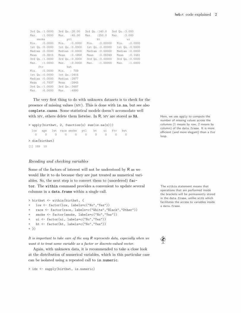
We then use box-and-whiskers charts to summarize each distribu-

tion. Note that we have rescaled them to avoid the problem of varying

y-axis.

> boxplot(apply(birthwt[,idx], 2, scale))

●

●

●

●

●

●

●

●●

●●

●

●●

●●●

●

●

●

●

●

●

●

●●●●●

●

●

●

●●●●●●●●●●●●

●●●

●

●

●●

●

●

●●●

●

age lwt ptl ftv bwt

−2

02

46

Figure 1: Parallel box and whiskerscharts.

Summarizing data

Most base functions in R can be used to summarize our variables,

either numerically or graphically. We have already seen the useful

summary command. For numerical variables, it will output a five-

number summary; for categorical data, a frequency of counts. In both

cases, missing cases will be reported separately. However, there is a

full set of dedicated tools included in the Hmisc package, especially the

summary.formula command.

> library(Hmisc)

> summary(low ~ ., data=birthwt, method="reverse", overall=TRUE)

> summary(bwt ~ ., data=birthwt)

The added functionalities proposedin the Hmisc package are oversizedcompared to most R packages. To usesome of the most powerful commands,it will be necessary to read carefully theon-line help.

> summary(low ~ smoke + ht + ui, data=birthwt, fun=table)

low N=189

+-------+---+---+---+---+

| | |N |No |Yes|

+-------+---+---+---+---+

|smoke |No |115| 86|29 |

| |Yes| 74| 44|30 |

+-------+---+---+---+---+

|ht |No |177|125|52 |

| |Yes| 12| 5| 7 |

+-------+---+---+---+---+

|ui |No |161|116|45 |

| |Yes| 28| 14|14 |

+-------+---+---+---+---+

|Overall| |189|130|59 |

+-------+---+---+---+---+

The above commands might be combined with the latex function

to produce pretty-print output, which follow standards for publications

in biomedical journal.

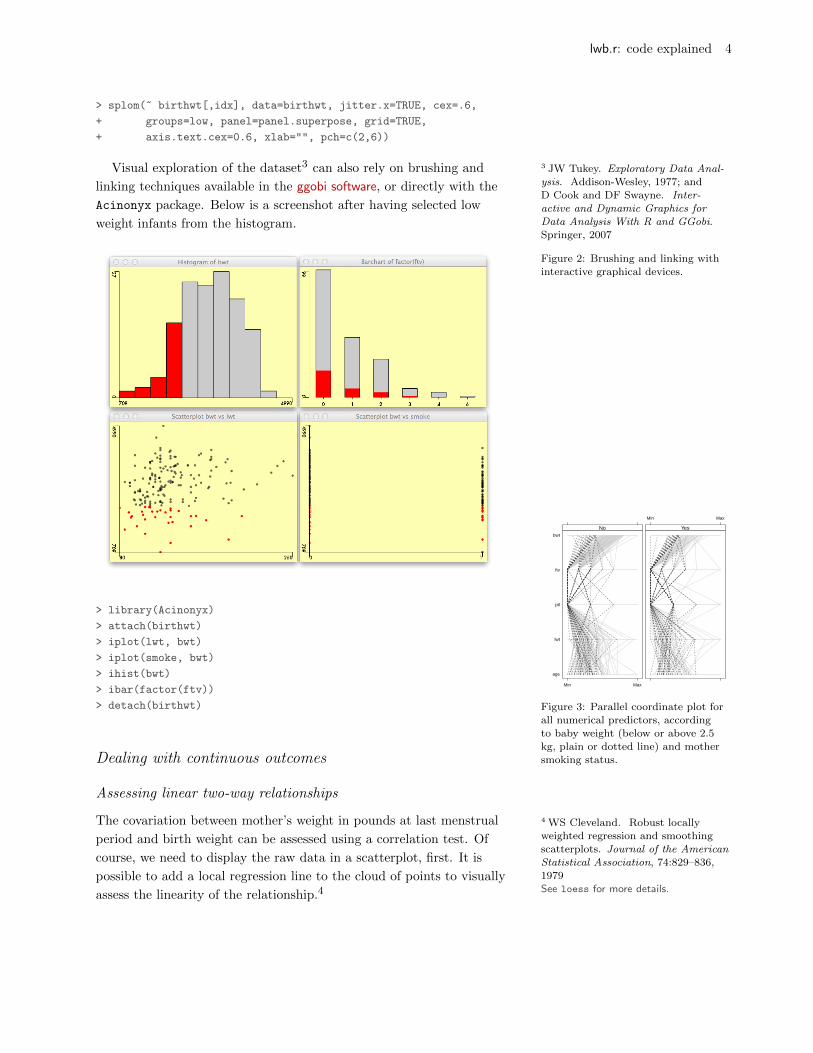
Multivariate displays can be used, essentially to study relation-

ships between numerical variables or assess any systematic patterns of

covariations. At this stage, it might be interesting to highlight individ-

uals according to a certain characteristic (e.g., low birth weight).

> library(lattice)

> parallel(birthwt[,idx], groups=birthwt$low, horizontal.axis=FALSE)

> print(parallel(~ birthwt[,idx] | smoke, data=birthwt, groups=low,

+ lty=1:2, col=c("gray80","gray20")))

http://biostat.mc.vanderbilt.edu/wiki/Main/RS


> splom(~ birthwt[,idx], data=birthwt, jitter.x=TRUE, cex=.6,

+ groups=low, panel=panel.superpose, grid=TRUE,

+ axis.text.cex=0.6, xlab="", pch=c(2,6))

Visual exploration of the dataset3 can also rely on brushing and 3 JW Tukey. Exploratory Data Anal-

ysis. Addison-Wesley, 1977; and

D Cook and DF Swayne. Inter-active and Dynamic Graphics for

Data Analysis With R and GGobi.

Springer, 2007

linking techniques available in the ggobi software, or directly with the

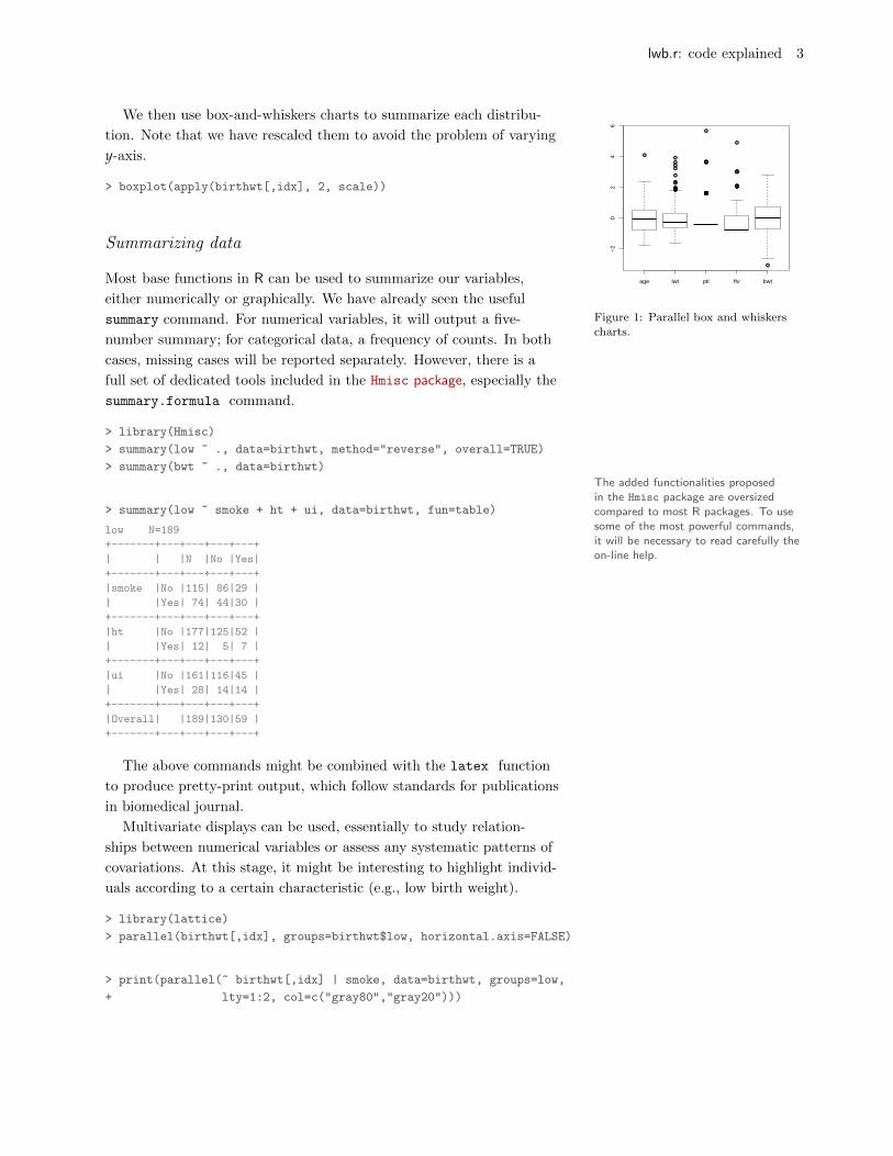
Acinonyx package. Below is a screenshot after having selected low

weight infants from the histogram.

Figure 2: Brushing and linking with

interactive graphical devices.

> library(Acinonyx)

> attach(birthwt)

> iplot(lwt, bwt)

> iplot(smoke, bwt)

> ihist(bwt)

> ibar(factor(ftv))

> detach(birthwt)

age

lwt

ptl

ftv

bwt

Min Max

No

Min Max

Yes

Figure 3: Parallel coordinate plot for

all numerical predictors, accordingto baby weight (below or above 2.5

kg, plain or dotted line) and mothersmoking status.Dealing with continuous outcomes

Assessing linear two-way relationships

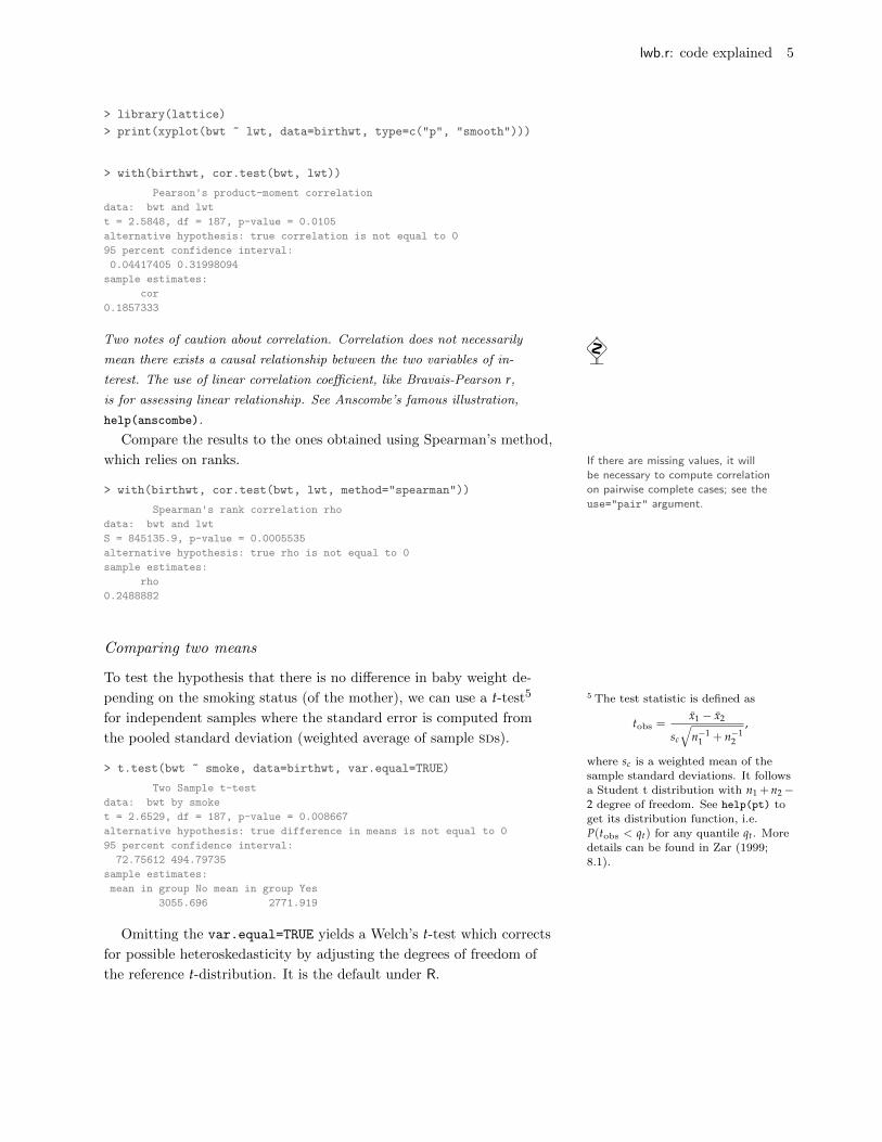
The covariation between mother’s weight in pounds at last menstrual

period and birth weight can be assessed using a correlation test. Of

course, we need to display the raw data in a scatterplot, first. It is

possible to add a local regression line to the cloud of points to visually

assess the linearity of the relationship.4

4 WS Cleveland. Robust locallyweighted regression and smoothingscatterplots. Journal of the American

Statistical Association, 74:829–836,1979

See loess for more details.

http://www.ggobi.org/


> library(lattice)

> print(xyplot(bwt ~ lwt, data=birthwt, type=c("p", "smooth")))

> with(birthwt, cor.test(bwt, lwt))

Pearson's product-moment correlation

data: bwt and lwt

t = 2.5848, df = 187, p-value = 0.0105

alternative hypothesis: true correlation is not equal to 0

95 percent confidence interval:

0.04417405 0.31998094

sample estimates:

cor

0.1857333

lwt

bwt

1000

2000

3000

4000

5000

100 150 200 250

●●●●● ●●● ●●● ●● ●●●● ●●●●● ●●● ●● ● ●●●● ● ●● ●●

●●● ● ●● ●●● ●●●● ● ●●● ●●● ●● ●●●● ●● ●● ●● ●● ●●● ● ●●●● ●● ●

●●

●●● ● ●● ●● ●● ●● ●●●●● ●●● ● ●● ●● ● ●● ●● ●●●●●● ●

●●●●

● ●●

●

●

●

●

●

●

●

●●

● ●●●

● ● ●● ● ●●●●● ● ● ● ●●●

●●● ●● ● ●● ●●● ● ● ●●● ● ● ●●●● ● ●● ●●● ●● ●●

Figure 4: A simple scatterplot with a

local smoother.

Two notes of caution about correlation. Correlation does not necessarily �

mean there exists a causal relationship between the two variables of in-

terest. The use of linear correlation coefficient, like Bravais-Pearson r,

is for assessing linear relationship. See Anscombe’s famous illustration,

help(anscombe).

Compare the results to the ones obtained using Spearman’s method,

which relies on ranks. If there are missing values, it willbe necessary to compute correlationon pairwise complete cases; see theuse="pair" argument.

> with(birthwt, cor.test(bwt, lwt, method="spearman"))

Spearman's rank correlation rho

data: bwt and lwt

S = 845135.9, p-value = 0.0005535

alternative hypothesis: true rho is not equal to 0

sample estimates:

rho

0.2488882

Comparing two means

To test the hypothesis that there is no difference in baby weight de-

pending on the smoking status (of the mother), we can use a t-test5 5 The test statistic is defined as

tobs =x1 − x2

sc

√n−1

1 + n−12

,

where sc is a weighted mean of thesample standard deviations. It followsa Student t distribution with n1 + n2−2 degree of freedom. See help(pt) to

get its distribution function, i.e.P(tobs < qt) for any quantile qt. More

details can be found in Zar (1999;8.1).

for independent samples where the standard error is computed from

the pooled standard deviation (weighted average of sample sds).

> t.test(bwt ~ smoke, data=birthwt, var.equal=TRUE)

Two Sample t-test

data: bwt by smoke

t = 2.6529, df = 187, p-value = 0.008667

alternative hypothesis: true difference in means is not equal to 0


72.75612 494.79735

sample estimates:

mean in group No mean in group Yes

3055.696 2771.919

Omitting the var.equal=TRUE yields a Welch’s t-test which corrects

for possible heteroskedasticity by adjusting the degrees of freedom of

the reference t-distribution. It is the default under R.


> t.test(bwt ~ smoke, data=birthwt)

Welch Two Sample t-test

data: bwt by smoke

t = 2.7299, df = 170.1, p-value = 0.007003

alternative hypothesis: true difference in means is not equal to 0


78.57486 488.97860

sample estimates:

mean in group No mean in group Yes

3055.696 2771.919

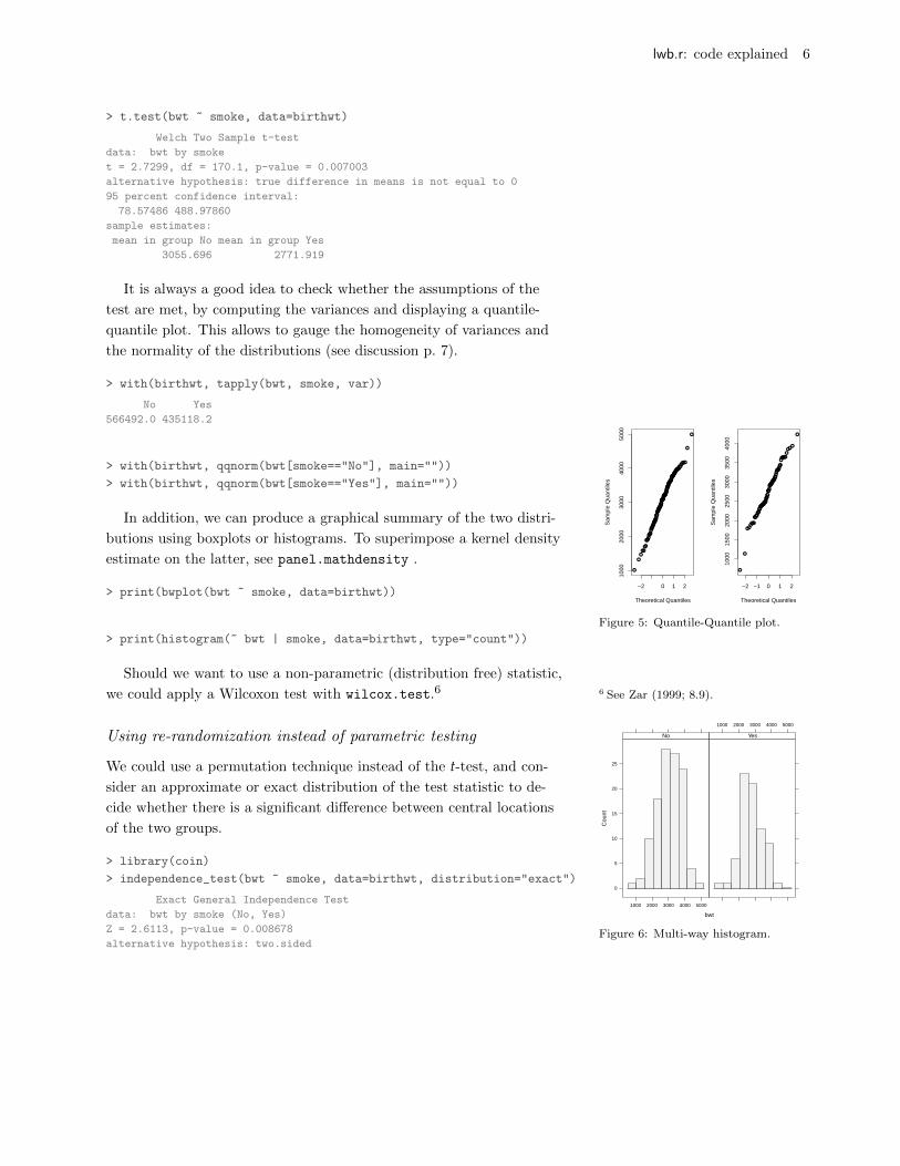
It is always a good idea to check whether the assumptions of the

test are met, by computing the variances and displaying a quantile-

quantile plot. This allows to gauge the homogeneity of variances and

the normality of the distributions (see discussion p. 7).

> with(birthwt, tapply(bwt, smoke, var))

No Yes

566492.0 435118.2

> with(birthwt, qqnorm(bwt[smoke=="No"], main=""))

> with(birthwt, qqnorm(bwt[smoke=="Yes"], main=""))

●●●●●●●●●●●●●●●●●●●●●●●●●●●●●●●●●●●●●●●●●●●●●●●●●●●●●●●●●●●●●●●●●●●●●●●●●●●●

●●●●●●

●●

●

●

●

●

●●●

●●

●●●●●●●●●●●●●●●●●●●●●●

−2 0 1 2

1000

2000

3000

4000

5000

Theoretical QuantilesS

ampl

e Q

uant

iles

●●●●●●●●●●●●●●●

●●●●●●●●●●●●●●●●●●

●●●●●●

●●●

●

●

●

●

●●●●●

●

●●●●●●●●●●●●●●●●●●●●●●

−2 −1 0 1 2

1000

1500

2000

2500

3000

3500

4000

Theoretical Quantiles

Sam

ple

Qua

ntile

s

Figure 5: Quantile-Quantile plot.

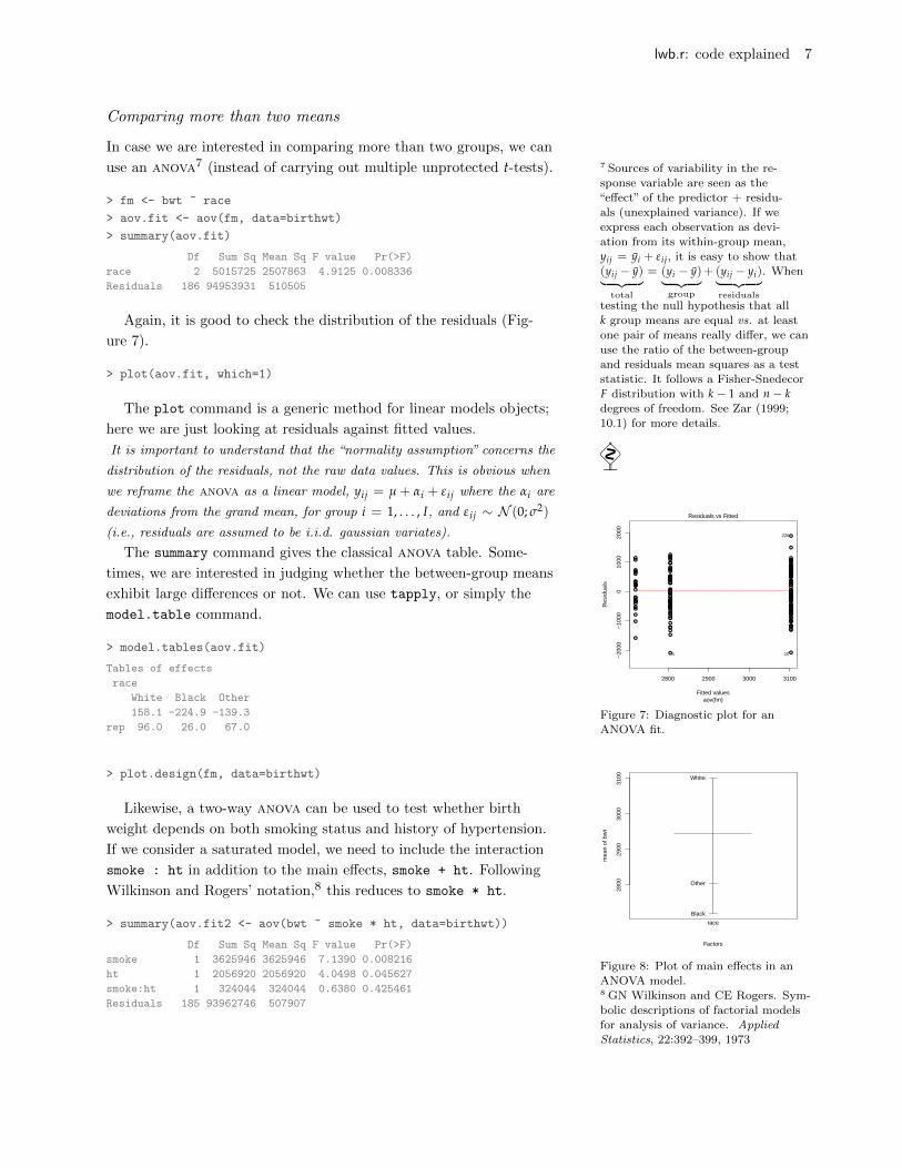
In addition, we can produce a graphical summary of the two distri-

butions using boxplots or histograms. To superimpose a kernel density

estimate on the latter, see panel.mathdensity .

> print(bwplot(bwt ~ smoke, data=birthwt))

> print(histogram(~ bwt | smoke, data=birthwt, type="count"))

Should we want to use a non-parametric (distribution free) statistic,

we could apply a Wilcoxon test with wilcox.test.6 6 See Zar (1999; 8.9).

bwt

Cou

nt

0

5

10

15

20

25

1000 2000 3000 4000 5000

No

1000 2000 3000 4000 5000

Yes

Figure 6: Multi-way histogram.

Using re-randomization instead of parametric testing

We could use a permutation technique instead of the t-test, and con-

sider an approximate or exact distribution of the test statistic to de-

cide whether there is a significant difference between central locations

of the two groups.

> library(coin)

> independence_test(bwt ~ smoke, data=birthwt, distribution="exact")

Exact General Independence Test

data: bwt by smoke (No, Yes)

Z = 2.6113, p-value = 0.008678

alternative hypothesis: two.sided


Comparing more than two means

In case we are interested in comparing more than two groups, we can

use an anova7 (instead of carrying out multiple unprotected t-tests). 7 Sources of variability in the re-

sponse variable are seen as the“effect” of the predictor + residu-

als (unexplained variance). If we

express each observation as devi-ation from its within-group mean,

yij = yi + εij, it is easy to show that(yij − y)︸︷︷︸

total

= (yi − y)︸︷︷︸group

+ (yij − yi)︸︷︷︸residuals

. When

testing the null hypothesis that allk group means are equal vs. at least

one pair of means really differ, we can

use the ratio of the between-groupand residuals mean squares as a test

statistic. It follows a Fisher-Snedecor

F distribution with k − 1 and n − kdegrees of freedom. See Zar (1999;

10.1) for more details.

> fm <- bwt ~ race

> aov.fit <- aov(fm, data=birthwt)

> summary(aov.fit)

Df Sum Sq Mean Sq F value Pr(>F)

race 2 5015725 2507863 4.9125 0.008336

Residuals 186 94953931 510505

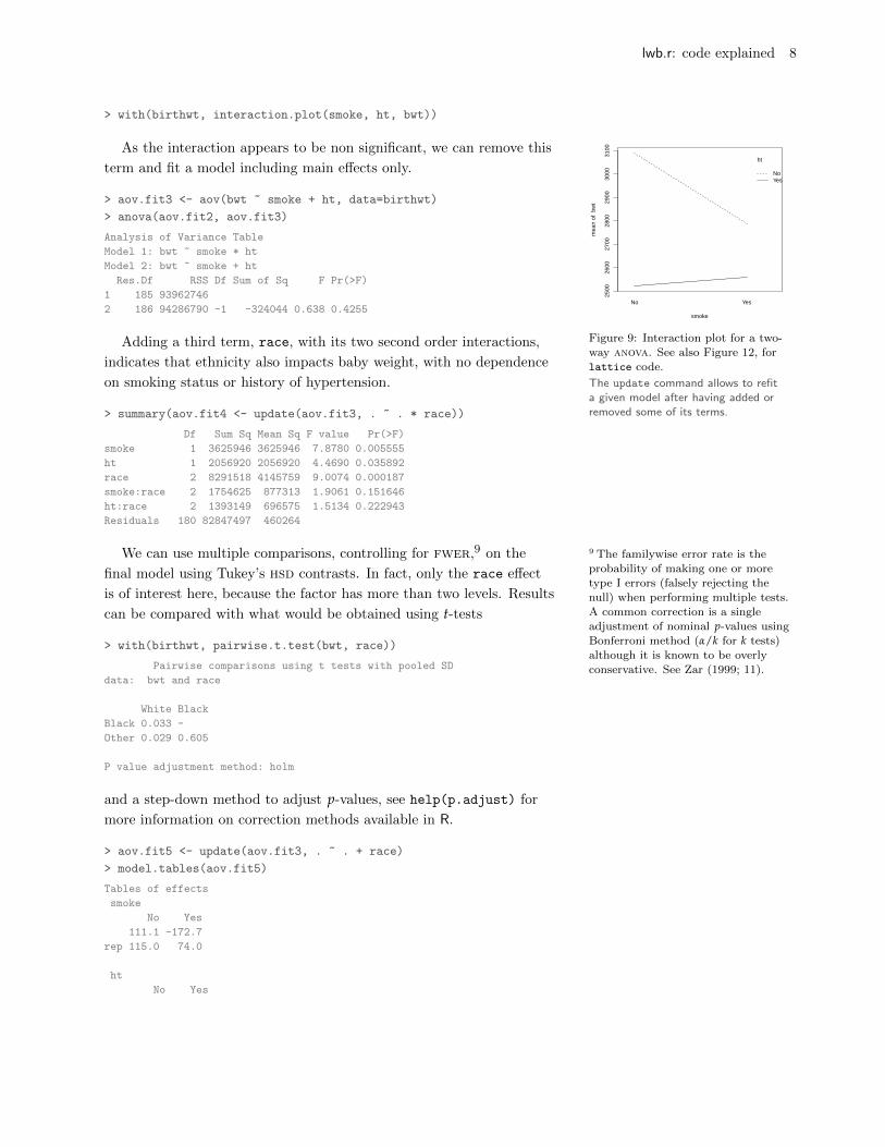
Again, it is good to check the distribution of the residuals (Fig-

ure 7).

> plot(aov.fit, which=1)

The plot command is a generic method for linear models objects;

here we are just looking at residuals against fitted values.

It is important to understand that the “normality assumption” concerns the �

distribution of the residuals, not the raw data values. This is obvious when

we reframe the anova as a linear model, yij = µ + αi + εij where the αi are

deviations from the grand mean, for group i = 1, . . . , I, and εij ∼ N (0; σ2)

(i.e., residuals are assumed to be i.i.d. gaussian variates).

The summary command gives the classical anova table. Some-

times, we are interested in judging whether the between-group means

exhibit large differences or not. We can use tapply, or simply the

model.table command.

2800 2900 3000 3100

−20

00−

1000

010

0020

00

Fitted values

Res

idua

ls● ●

●●●

●

●

●

●●

●●●●

●●

●

●

●

●

●

●●

●●

●●●

●●●

●

●

●

●

●●●●●

●

●

●

●●●●

●

●

●

●

●

●●

●●●●●●●●●

●

●●●●

●

●

●

●●●

●

●

●●

●

●●●

●●●●●

●●●●

●

●●●●●●●●●●

●

●

●●

●●●

●

●

●

●●●

●

●

●

●

●

●

●

●●●●●●

●

●

● ●

●●●●●

● ●

●●●

●●

●●

●

●

●●●

●●●●

●●

●

●●

●

●●●●

●

●●

●●

●●●●●

●●●●

●●●

●

●

●

●●●

●

aov(fm)

Residuals vs Fitted

4 10

226

Figure 7: Diagnostic plot for an

ANOVA fit.

> model.tables(aov.fit)

Tables of effects

race

White Black Other

158.1 -224.9 -139.3

rep 96.0 26.0 67.0

> plot.design(fm, data=birthwt)

2800

2900

3000

3100

Factors

mea

n of

bw

t

White

Black

Other

race

Figure 8: Plot of main effects in an

ANOVA model.

Likewise, a two-way anova can be used to test whether birth

weight depends on both smoking status and history of hypertension.

If we consider a saturated model, we need to include the interaction

smoke : ht in addition to the main effects, smoke + ht. Following

Wilkinson and Rogers’ notation,8 this reduces to smoke * ht.

8 GN Wilkinson and CE Rogers. Sym-bolic descriptions of factorial models

for analysis of variance. Applied

Statistics, 22:392–399, 1973

> summary(aov.fit2 <- aov(bwt ~ smoke * ht, data=birthwt))


smoke 1 3625946 3625946 7.1390 0.008216

ht 1 2056920 2056920 4.0498 0.045627

smoke:ht 1 324044 324044 0.6380 0.425461

Residuals 185 93962746 507907


> with(birthwt, interaction.plot(smoke, ht, bwt))

2500

2600

2700

2800

2900

3000

3100

smoke

mea

n of

bw

t

No Yes

ht

NoYes

Figure 9: Interaction plot for a two-way anova. See also Figure 12, for

lattice code.

As the interaction appears to be non significant, we can remove this

term and fit a model including main effects only.

> aov.fit3 <- aov(bwt ~ smoke + ht, data=birthwt)

> anova(aov.fit2, aov.fit3)

Analysis of Variance Table

Model 1: bwt ~ smoke * ht

Model 2: bwt ~ smoke + ht

Res.Df RSS Df Sum of Sq F Pr(>F)

1 185 93962746

2 186 94286790 -1 -324044 0.638 0.4255

Adding a third term, race, with its two second order interactions,

indicates that ethnicity also impacts baby weight, with no dependence

on smoking status or history of hypertension. The update command allows to refita given model after having added orremoved some of its terms.> summary(aov.fit4 <- update(aov.fit3, . ~ . * race))


smoke 1 3625946 3625946 7.8780 0.005555

ht 1 2056920 2056920 4.4690 0.035892

race 2 8291518 4145759 9.0074 0.000187

smoke:race 2 1754625 877313 1.9061 0.151646

ht:race 2 1393149 696575 1.5134 0.222943

Residuals 180 82847497 460264

We can use multiple comparisons, controlling for fwer,9 on the 9 The familywise error rate is theprobability of making one or more

type I errors (falsely rejecting the

null) when performing multiple tests.A common correction is a single

adjustment of nominal p-values usingBonferroni method (α/k for k tests)

although it is known to be overly

conservative. See Zar (1999; 11).

final model using Tukey’s hsd contrasts. In fact, only the race effect

is of interest here, because the factor has more than two levels. Results

can be compared with what would be obtained using t-tests

> with(birthwt, pairwise.t.test(bwt, race))

Pairwise comparisons using t tests with pooled SD

data: bwt and race

White Black

Black 0.033 -

Other 0.029 0.605

P value adjustment method: holm

and a step-down method to adjust p-values, see help(p.adjust) for

more information on correction methods available in R.

> aov.fit5 <- update(aov.fit3, . ~ . + race)

> model.tables(aov.fit5)

Tables of effects

smoke

No Yes

111.1 -172.7

rep 115.0 74.0

ht

No Yes


27.16 -400.6

rep 177.00 12.0

race

White Black Other

195.4 -204.6 -200.6

rep 96.0 26.0 67.0

> se.contrast(aov.fit5, list(birthwt$race=="White",

+ birthwt$race=="Black"))

[1] 151.1423

> TukeyHSD(aov.fit5, which="race")

Tukey multiple comparisons of means

95% family-wise confidence level

Fit: aov(formula = bwt ~ smoke + ht + race, data = birthwt)

$race

diff lwr upr p adj

Black-White -400.059794 -757.1842 -42.93537 0.0238683

Other-White -396.023345 -653.1711 -138.87560 0.0010320

Other-Black 4.036449 -369.1959 377.26884 0.9996401

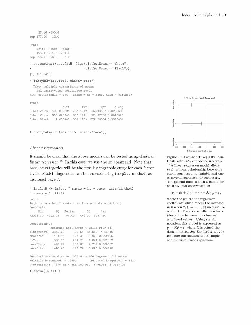
> plot(TukeyHSD(aov.fit5, which="race"))

−800 −600 −400 −200 0 200 400Oth

er−

Bla

ckO

ther

−W

hite

Bla

ck−

Whi

te

95% family−wise confidence level

Differences in mean levels of race

Figure 10: Post-hoc Tukey’s hsd con-trasts with 95% confidence intervals.

Linear regression

It should be clear that the above models can be tested using classical

linear regression.10 In this case, we use the lm command. Note that10 A linear regression model allows

to fit a linear relationship between a

continuous response variable and oneor several regressors, or predictors.

The general form of such a model foran individual observation is:

yi = β0 + β1xi1 + · · ·+ βpxip + εi ,

where the β’s are the regression

coefficients which reflect the increasein y when xj (j = 1, . . . , p) increases by

one unit. The ε’s are called residuals

(deviations between the observedand fitted values). Using matrixnotation, this model is expressed asy = Xβ + ε, where X is coined thedesign matrix. See Zar (1999; 17, 20)

for more information about simpleand multiple linear regression.

baseline categories will be the first lexicographic entry for each factor

levels. Model diagnostics can be assessed using the plot method, as

discussed page 7.

> lm.fit5 <- lm(bwt ~ smoke + ht + race, data=birthwt)

> summary(lm.fit5)

Call:

lm(formula = bwt ~ smoke + ht + race, data = birthwt)

Residuals:

Min 1Q Median 3Q Max

-2331.70 -462.03 -6.03 474.30 1637.30

Coefficients:

Estimate Std. Error t value Pr(>|t|)

(Intercept) 3352.70 91.65 36.580 < 2e-16

smokeYes -424.68 108.33 -3.920 0.000125

htYes -383.06 204.73 -1.871 0.062932

raceBlack -425.47 152.68 -2.787 0.005882

raceOther -448.49 115.72 -3.876 0.000148

Residual standard error: 683.6 on 184 degrees of freedom

Multiple R-squared: 0.1398, Adjusted R-squared: 0.1211

F-statistic: 7.475 on 4 and 184 DF, p-value: 1.335e-05

> anova(lm.fit5)


Analysis of Variance Table

Response: bwt


smoke 1 3625946 3625946 7.7583 0.005906

ht 1 2056920 2056920 4.4011 0.037282

race 2 8291518 4145759 8.8705 0.000210

Residuals 184 85995271 467366

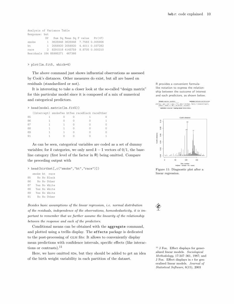
> plot(lm.fit5, which=4)

The above command just shows influential observations as assessed

by Cook’s distances. Other measures do exist, but all are based on

residuals (standardized or not). R provides a convenient formula-like notation to express the relation-ship between the outcome of interestand each predictors, as shown below.

glm(low ~ age + lwt + race + ftv, data = birthwt, family = binomial(logit), subset = smoke == "No", na.action = na.omit)

formula: response ~ predictors residuals: distribution and link function

missing values: listwise deletionrestriction: subsample

0 50 100 1500.

000.

020.

040.

060.

080.

10

Obs. number

Coo

k's

dist

ance

lm(bwt ~ smoke + ht + race)

Cook's distance

202

19713

Figure 11: Diagnostic plot after a

linear regression.

It is interesting to take a closer look at the so-called “design matrix”

for this particular model since it is composed of a mix of numerical

and categorical predictors.

> head(model.matrix(lm.fit5))

(Intercept) smokeYes htYes raceBlack raceOther

85 1 0 0 1 0

86 1 0 0 0 1

87 1 1 0 0 0

88 1 1 0 0 0

89 1 1 0 0 0

91 1 0 0 0 1

As can be seen, categorical variables are coded as a set of dummy

variables; for k categories, we only need k− 1 vectors of 0/1, the base-

line category (first level of the factor in R) being omitted. Compare

the preceding output with

> head(birthwt[,c("smoke","ht","race")])

smoke ht race

85 No No Black

86 No No Other

87 Yes No White

88 Yes No White

89 Yes No White

91 No No Other

Besides basic assumptions of the linear regression, i.e. normal distribution �

of the residuals, independence of the observations, homoskedasticity, it is im-

portant to remember that we further assume the linearity of the relationship

between the response and each of the predictors.

Conditional means can be obtained with the aggregate command,

and plotted using a trellis display. The effects package is dedicated

to the post-processing of glm fits: It allows to conveniently display

mean predictions with confidence intervals, specific effects (like interac-

tions or contrasts).11 11 J Fox. Effect displays for gener-

alized linear models. SociologicalMethodology, 17:347–361, 1987; and

J Fox. Effect displays in r for gen-

eralised linear models. Journal ofStatistical Software, 8(15), 2003

Here, we have omitted sds, but they should be added to get an idea

of the birth weight variability in each partition of the dataset.


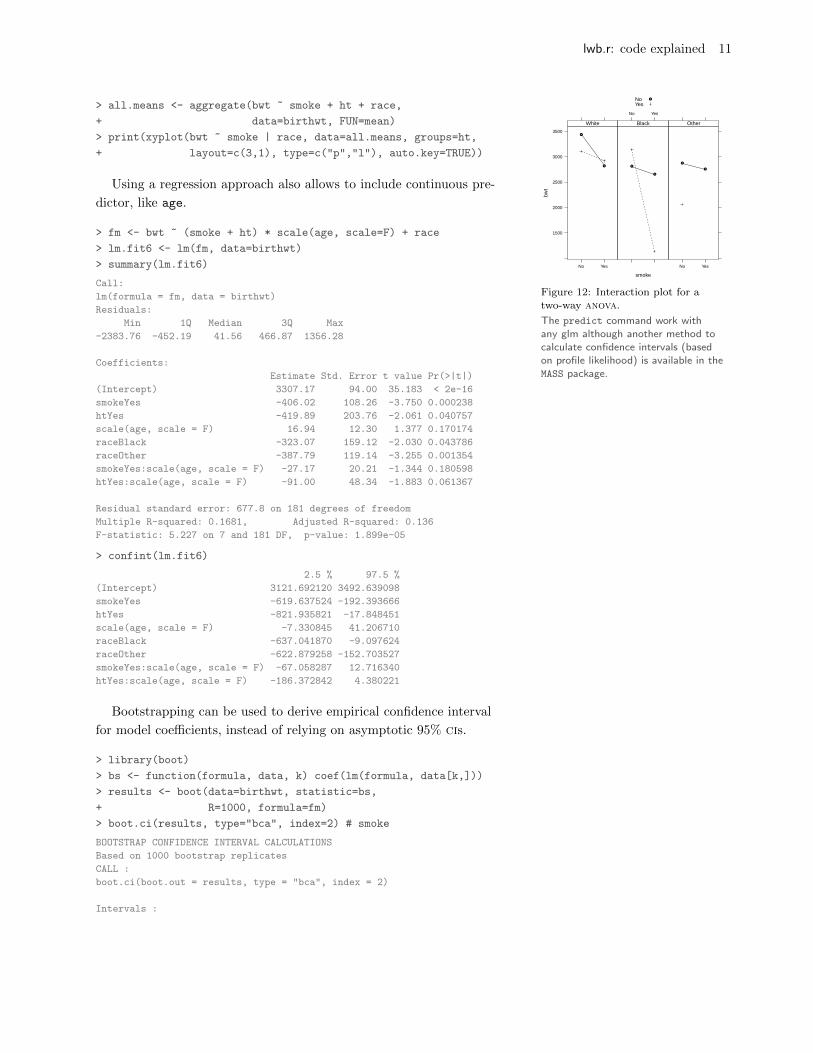
> all.means <- aggregate(bwt ~ smoke + ht + race,

+ data=birthwt, FUN=mean)

> print(xyplot(bwt ~ smoke | race, data=all.means, groups=ht,

+ layout=c(3,1), type=c("p","l"), auto.key=TRUE))

smoke

bwt

1500

2000

2500

3000

3500

No Yes

●

●

White

No Yes

●

●

Black

No Yes

●

●

Other

NoYes

●

Figure 12: Interaction plot for a

two-way anova.

Using a regression approach also allows to include continuous pre-

dictor, like age.

The predict command work withany glm although another method tocalculate confidence intervals (basedon profile likelihood) is available in theMASS package.

> fm <- bwt ~ (smoke + ht) * scale(age, scale=F) + race

> lm.fit6 <- lm(fm, data=birthwt)

> summary(lm.fit6)

Call:

lm(formula = fm, data = birthwt)

Residuals:


-2383.76 -452.19 41.56 466.87 1356.28

Coefficients:


(Intercept) 3307.17 94.00 35.183 < 2e-16

smokeYes -406.02 108.26 -3.750 0.000238

htYes -419.89 203.76 -2.061 0.040757

scale(age, scale = F) 16.94 12.30 1.377 0.170174

raceBlack -323.07 159.12 -2.030 0.043786

raceOther -387.79 119.14 -3.255 0.001354

smokeYes:scale(age, scale = F) -27.17 20.21 -1.344 0.180598

htYes:scale(age, scale = F) -91.00 48.34 -1.883 0.061367




> confint(lm.fit6)

2.5 % 97.5 %

(Intercept) 3121.692120 3492.639098

smokeYes -619.637524 -192.393666

htYes -821.935821 -17.848451

scale(age, scale = F) -7.330845 41.206710

raceBlack -637.041870 -9.097624

raceOther -622.879258 -152.703527

smokeYes:scale(age, scale = F) -67.058287 12.716340

htYes:scale(age, scale = F) -186.372842 4.380221

Bootstrapping can be used to derive empirical confidence interval

for model coefficients, instead of relying on asymptotic 95% cis.

> library(boot)

> bs <- function(formula, data, k) coef(lm(formula, data[k,]))

> results <- boot(data=birthwt, statistic=bs,

+ R=1000, formula=fm)

> boot.ci(results, type="bca", index=2) # smoke

BOOTSTRAP CONFIDENCE INTERVAL CALCULATIONS

Based on 1000 bootstrap replicates

CALL :

boot.ci(boot.out = results, type = "bca", index = 2)

Intervals :


Level BCa

95% (-599.3, -174.2 )

Calculations and Intervals on Original Scale

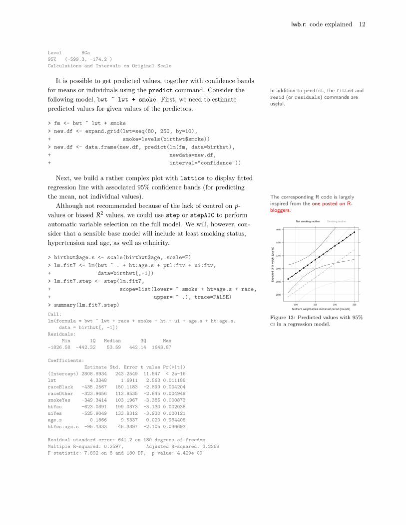
It is possible to get predicted values, together with confidence bands

for means or individuals using the predict command. Consider the In addition to predict, the fitted andresid (or residuals) commands areuseful.

following model, bwt ~ lwt + smoke. First, we need to estimate

predicted values for given values of the predictors.

> fm <- bwt ~ lwt + smoke

> new.df <- expand.grid(lwt=seq(80, 250, by=10),

+ smoke=levels(birthwt$smoke))

> new.df <- data.frame(new.df, predict(lm(fm, data=birthwt),

+ newdata=new.df,

+ interval="confidence"))

Next, we build a rather complex plot with lattice to display fitted

regression line with associated 95% confidence bands (for predicting

the mean, not individual values). The corresponding R code is largelyinspired from the one posted on R-bloggers.

Mother's weight at last menstrual period (pounds)

Exp

ecte

d bi

rth

wei

ght (

gram

s)

2600

2800

3000

3200

3400

3600

100 150 200 250

●

●

●

●

●

●

●

●

●

●

●

●

●

●

●

●

●

●

Not smoking mother Smoking mother

Figure 13: Predicted values with 95%

ci in a regression model.

Although not recommended because of the lack of control on p-

values or biased R2 values, we could use step or stepAIC to perform

automatic variable selection on the full model. We will, however, con-

sider that a sensible base model will include at least smoking status,

hypertension and age, as well as ethnicity.

> birthwt$age.s <- scale(birthwt$age, scale=F)

> lm.fit7 <- lm(bwt ~ . + ht:age.s + ptl:ftv + ui:ftv,

+ data=birthwt[,-1])

> lm.fit7.step <- step(lm.fit7,

+ scope=list(lower= ~ smoke + ht*age.s + race,

+ upper= ~ .), trace=FALSE)

> summary(lm.fit7.step)

Call:

lm(formula = bwt ~ lwt + race + smoke + ht + ui + age.s + ht:age.s,

data = birthwt[, -1])

Residuals:


-1826.58 -442.32 53.59 442.14 1643.87

Coefficients:


(Intercept) 2808.8934 243.2549 11.547 < 2e-16

lwt 4.3348 1.6911 2.563 0.011188

raceBlack -435.2567 150.1183 -2.899 0.004204

raceOther -323.9656 113.8535 -2.845 0.004949

smokeYes -349.3414 103.1967 -3.385 0.000873

htYes -623.0391 199.0373 -3.130 0.002038

uiYes -525.9049 133.8312 -3.930 0.000121

age.s 0.1866 9.5337 0.020 0.984408

htYes:age.s -95.4333 45.3397 -2.105 0.036693




http://www.r-bloggers.com/confidence-bands-with-lattice-and-r/

http://www.r-bloggers.com/confidence-bands-with-lattice-and-r/


A better way to perform variable selection is through penalization,

i.e. shrinkage of regression coefficients to zero or use of penalized

likelihood.12 12 Stepwise methods are unstable,

yield biased estimation of regressioncoefficients and misspecified estimates

of variability, but above all there is no

control on p-values. See Steyerberg(2009; 11.7) for alternative ways of

performing variable selection.

Dealing with categorical outcomes

Comparing two proportions

Considering the cross-classification of the existence of previous pre-

mature labours (yes/no) with number of physician visits during the

first trimester (1 or more than one), we can ask whether there is any

association between the two variables using a chi-square test.

> ptd <- factor(birthwt$ptl > 0, labels=c("No","Yes"))

> ftv2 <- factor(ifelse(birthwt$ftv < 2, "1", "2+"))

> tab.ptd.ftv <- table(ptd, ftv2)

> prop.table(tab.ptd.ftv, 1)

ftv2

ptd 1 2+

No 0.7610063 0.2389937

Yes 0.8666667 0.1333333

> chisq.test(tab.ptd.ftv)

Pearson's Chi-squared test with Yates' continuity correction

data: tab.ptd.ftv

X-squared = 1.0762, df = 1, p-value = 0.2996

It is usually recommended that expected cell frequencies should be > 5 for �

the χ2 test to be valid, although this criterion has been shown to be very

stringent. On a related point, Yates’ correction for continuity in χ2 tests

results in tests that are more conservative as with Fisher’s “exact” tests.

Finally, choosing between χ2 and Fisher test depends on the question that is

asked and the assumptions that are made by each of them (e.g., in the case

of the Fisher’s test we assume that margins are fixed).13 13 I Campbell. Chi-squared and

Fisher-Irwin tests of two-by-two tableswith small sample recommendations.Statistics in Medicine, 26(19):3661–

3675, 2007; and MG Haviland. Yates’scorrection for continuity and the

analysis of 2× 2 contingency tables.

Statistics in Medicine, 9(4):363–367,1990

More association measures are available through the assocstats

function in the vcd package. This package also features original graph-

ical displays for categorical data.14

14 M Friendly. Visualizing Categorical

Data. SAS Institute Inc., 2000

In particular, we could test for an association between smoking

status (considered here as an exposure factor) and a low-weight in-

fant (low), optionally considering ethnicity as a stratification factor.

A Cochran-Mantel-Haenszel test15 can be used to derive a common15 The CMH estimator is a weighted

average of stratum-specific or, defined

as

OR =∑i ai × di/Ni

∑i bi × ci/Ni ,where the a, b, c, d corresponds to

individual cells in stratum i of theform

(a bc d

)(e.g., low birth weight

status in rows and smoking status in

columns). It follows a χ2 distributionwith one degree of freedom.

odds-ratio estimate for low baby weight by smoking status, after strat-

ification on ethnicity.

Here is a simple estimate of the odds-ratio, ignoring the stratifica-

tion factor:

> library(vcd)

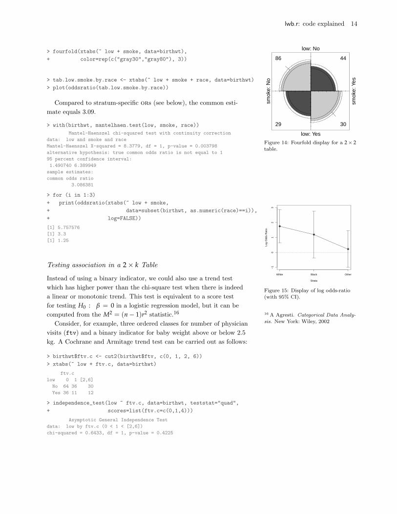
> oddsratio(xtabs(~ low + smoke, data=birthwt), log=FALSE)

[1] 2.021944


> fourfold(xtabs(~ low + smoke, data=birthwt),

+ color=rep(c("gray30","gray80"), 3))

low: No

smok

e: N

o

low: Yes

smok

e: Y

es

86

29

44

30

Figure 14: Fourfold display for a 2× 2table.

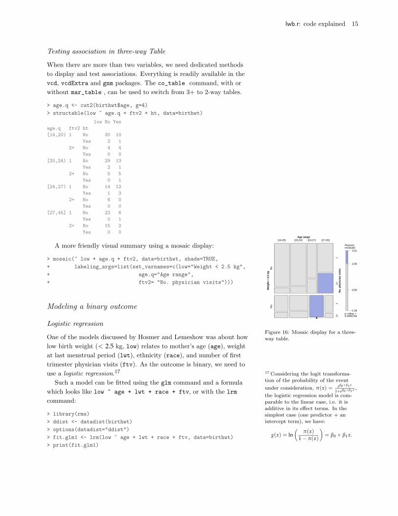
> tab.low.smoke.by.race <- xtabs(~ low + smoke + race, data=birthwt)

> plot(oddsratio(tab.low.smoke.by.race))

Compared to stratum-specific ors (see below), the common esti-

mate equals 3.09.

> with(birthwt, mantelhaen.test(low, smoke, race))

Mantel-Haenszel chi-squared test with continuity correction

data: low and smoke and race

Mantel-Haenszel X-squared = 8.3779, df = 1, p-value = 0.003798

alternative hypothesis: true common odds ratio is not equal to 1


1.490740 6.389949

sample estimates:

common odds ratio

3.086381

> for (i in 1:3)

+ print(oddsratio(xtabs(~ low + smoke,

+ data=subset(birthwt, as.numeric(race)==i)),

+ log=FALSE))

[1] 5.757576

[1] 3.3

[1] 1.25

●

●

●

−1

01

23

Strata

Log

Odd

s R

atio

White Black Other

Figure 15: Display of log odds-ratio(with 95% CI).

Testing association in a 2× k Table

Instead of using a binary indicator, we could also use a trend test

which has higher power than the chi-square test when there is indeed

a linear or monotonic trend. This test is equivalent to a score test

for testing H0 : β = 0 in a logistic regression model, but it can be

computed from the M2 = (n− 1)r2 statistic.16 16 A Agresti. Categorical Data Analy-

sis. New York: Wiley, 2002Consider, for example, three ordered classes for number of physician

visits (ftv) and a binary indicator for baby weight above or below 2.5

kg. A Cochrane and Armitage trend test can be carried out as follows:

> birthwt$ftv.c <- cut2(birthwt$ftv, c(0, 1, 2, 6))

> xtabs(~ low + ftv.c, data=birthwt)

ftv.c

low 0 1 [2,6]

No 64 36 30

Yes 36 11 12

> independence_test(low ~ ftv.c, data=birthwt, teststat="quad",

+ scores=list(ftv.c=c(0,1,4)))

Asymptotic General Independence Test

data: low by ftv.c (0 < 1 < [2,6])

chi-squared = 0.6433, df = 1, p-value = 0.4225


Testing association in three-way Table

When there are more than two variables, we need dedicated methods

to display and test associations. Everything is readily available in the

vcd, vcdExtra and gnm packages. The co_table command, with or

without mar_table , can be used to switch from 3+ to 2-way tables.

> age.q <- cut2(birthwt$age, g=4)

> structable(low ~ age.q + ftv2 + ht, data=birthwt)

low No Yes

age.q ftv2 ht

[14,20) 1 No 30 10

Yes 2 1

2+ No 4 4

Yes 0 0

[20,24) 1 No 29 13

Yes 2 1

2+ No 5 5

Yes 0 1

[24,27) 1 No 14 12

Yes 1 3

2+ No 6 0

Yes 0 0

[27,45] 1 No 22 6

Yes 0 1

2+ No 15 2

Yes 0 0

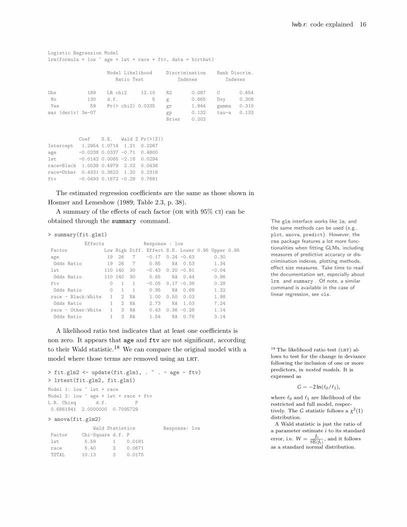
A more friendly visual summary using a mosaic display:

> mosaic(~ low + age.q + ftv2, data=birthwt, shade=TRUE,

+ labeling_args=list(set_varnames=c(low="Weight < 2.5 kg",

+ age.q="Age range",

+ ftv2= "No. physician visits")))

−1.58

0.00

2.00

3.01

Pearsonresiduals:

p−value =0.0056706

●●

Age range

Wei

ght <

2.5

kg

No.

phy

sici

an v

isits

Yes

2+1

No

[14,20) [20,24) [24,27) [27,45]

2+1

Figure 16: Mosaic display for a three-

way table.

Modeling a binary outcome

Logistic regression

One of the models discussed by Hosmer and Lemeshow was about how

low birth weight (< 2.5 kg, low) relates to mother’s age (age), weight

at last menstrual period (lwt), ethnicity (race), and number of first

trimester physician visits (ftv). As the outcome is binary, we need to

use a logistic regression.17 17 Considering the logit transforma-tion of the probability of the event

under consideration, π(x) = eβ0+β1 x

1+eβ0+β1 x ,

the logistic regression model is com-parable to the linear case, i.e. it is

additive in its effect terms. In thesimplest case (one predictor + an

intercept term), we have:

g(x) = ln(

π(x)

1− π(x)

)= β0 + β1x.

Such a model can be fitted using the glm command and a formula

which looks like low ~ age + lwt + race + ftv, or with the lrm

command:

> library(rms)

> ddist <- datadist(birthwt)

> options(datadist="ddist")

> fit.glm1 <- lrm(low ~ age + lwt + race + ftv, data=birthwt)

> print(fit.glm1)


Logistic Regression Model

lrm(formula = low ~ age + lwt + race + ftv, data = birthwt)

Model Likelihood Discrimination Rank Discrim.

Ratio Test Indexes Indexes

Obs 189 LR chi2 12.10 R2 0.087 C 0.654

No 130 d.f. 5 g 0.665 Dxy 0.308

Yes 59 Pr(> chi2) 0.0335 gr 1.944 gamma 0.310

max |deriv| 3e-07 gp 0.132 tau-a 0.133

Brier 0.202

Coef S.E. Wald Z Pr(>|Z|)

Intercept 1.2954 1.0714 1.21 0.2267

age -0.0238 0.0337 -0.71 0.4800

lwt -0.0142 0.0065 -2.18 0.0294

race=Black 1.0039 0.4979 2.02 0.0438

race=Other 0.4331 0.3622 1.20 0.2318

ftv -0.0493 0.1672 -0.29 0.7681

The estimated regression coefficients are the same as those shown in

Hosmer and Lemeshow (1989; Table 2.3, p. 38).

A summary of the effects of each factor (or with 95% ci) can be

obtained through the summary command. The glm interface works like lm, andthe same methods can be used (e.g.,plot, anova, predict). However, therms package features a lot more func-tionalities when fitting GLMs, includingmeasures of predictive accuracy or dis-crimination indexes, plotting methods,effect size measures. Take time to readthe documentation set, especially aboutlrm and summary . Of note, a similarcommand is available in the case oflinear regression, see ols.

> summary(fit.glm1)

Effects Response : low

Factor Low High Diff. Effect S.E. Lower 0.95 Upper 0.95

age 19 26 7 -0.17 0.24 -0.63 0.30

Odds Ratio 19 26 7 0.85 NA 0.53 1.34

lwt 110 140 30 -0.43 0.20 -0.81 -0.04

Odds Ratio 110 140 30 0.65 NA 0.44 0.96

ftv 0 1 1 -0.05 0.17 -0.38 0.28

Odds Ratio 0 1 1 0.95 NA 0.69 1.32

race - Black:White 1 2 NA 1.00 0.50 0.03 1.98

Odds Ratio 1 2 NA 2.73 NA 1.03 7.24

race - Other:White 1 3 NA 0.43 0.36 -0.28 1.14

Odds Ratio 1 3 NA 1.54 NA 0.76 3.14

A likelihood ratio test indicates that at least one coefficients is

non zero. It appears that age and ftv are not significant, according

to their Wald statistic.18 We can compare the original model with a 18 The likelihood ratio test (lrt) al-

lows to test for the change in deviancefollowing the inclusion of one or more

predictors, in nested models. It isexpressed as

G = −2 ln(`0/`1),

where `0 and `1 are likelihood of the

restricted and full model, respec-tively. The G statistic follows a χ2(1)distribution.

A Wald statistic is just the ratio ofa parameter estimate i to its standard

error, i.e. W = βiSE(βi)

, and it follows

as a standard normal distribution.

model where those terms are removed using an lrt.

> fit.glm2 <- update(fit.glm1, . ~ . - age - ftv)

> lrtest(fit.glm2, fit.glm1)

Model 1: low ~ lwt + race

Model 2: low ~ age + lwt + race + ftv

L.R. Chisq d.f. P

0.6861841 2.0000000 0.7095729

> anova(fit.glm2)

Wald Statistics Response: low

Factor Chi-Square d.f. P

lwt 5.59 1 0.0181

race 5.40 2 0.0671

TOTAL 10.13 3 0.0175


Finally, we could predict the expected outcome (with confidence

intervals for means) for a particular range of weight at last menstrual

period, depending on mother’s ethnicity.

> pred.glm2 <- Predict(fit.glm2, lwt=seq(80, 250, by=10), race)

> print(xYplot(Cbind(yhat,lower,upper) ~ lwt | race, data=pred.glm2,

+ method="filled bands", type="l", col.fill=gray(.95)))

lwt

yhat

−4

−3

−2

−1

0

1

100 150 200 250

White Black

−4

−3

−2

−1

0

1

Other

Figure 17: Predicted response on thelog odds scale for birth weight with

95% confidence bands.

Still on the log odds scale, we can predict the expected weight

category for a white mother’s of last menstrual weight lwt=150:

> Predict(fit.glm2, lwt=150, race="White")

lwt race yhat lower upper

1 150 White -1.477712 -2.042931 -0.9124926

Response variable (y): log odds

Limits are 0.95 confidence limits

Or we can use the regression equation directly since we have access

parameters estimates. The or is computed as:

> exp(sum(coef(fit.glm2)*c(1, 150, 0, 0)))

[1] 0.2281591

The above approach assumes we have a priori hypothesis concerning the �

variables to include in our model. Assuming no prior knowledge, it would be

necessary to perform some kind of variables selection, using e.g. a penalized

likelihood method (see the penalty parameter in lrm).19 19 KG Moons, AR Donders,

EW Steyerberg, and FE Harrell.

Penalized maximum likelihood esti-mation to predict binary outcomes.

Journal of Clinical Epidemiology, 57(12):1262–1270, 2004

What’s next?

Model diagnostic and model selection are important steps when build-

ing a predictive model, though it was not discussed here. A very thor-

ough review of relevant methods is available in Steyerberg (2009).

Details on the R version and packages used are given below:

• R version 2.13.2 (2011-09-30), x86_64-apple-darwin9.8.0

• Base packages: base, datasets, graphics, grDevices, grid, methods, splines, stats,stats4, utils

• Other packages: boot 1.3-2, coin 1.0-20, colorspace 1.1-1, Hmisc 3.8-3,lattice 0.19-34, MASS 7.3-14, modeltools 0.2-18, mvtnorm 0.9-9991, rms 3.3-1,

survival 2.36-10, vcd 1.2-12

• Loaded via a namespace (and not attached): cluster 1.14.0, tools 2.13.2

This document was typesetted in LATEX as lwb_explained.rnw, version 4911255 on

2011/10/24.

Index

aggregate, 10

anova, 16

apply, 2

assocstats (vcd package), 13

birthwt (MASS package), 1

co_table (vcd package), 15

complete.cases, 2

data, 1

factor, 2

fitted, 12

glm, 15, 16

is.na, 2

is.numeric, 2

latex (Hmisc package), 3

lm, 9, 16

loess, 4

lrm, 17

lrm (rms package), 15, 16

mar_table (vcd package), 15

model.table, 7

ols, 16

packages

Acinonyx, 4

effects, 10

foreign, 1

gnm, 15

Hmisc, 3

lattice, 1, 8, 12

MASS, 1, 11

rms, 16

vcd, 13, 15

vcdExtra, 15

panel.mathdensity (lattice pack-

age), 6

plot, 7, 9, 16

predict, 11, 12, 16

read.dta (foreign package), 1

resid, 12

residuals, 12

step, 12

stepAIC, 12

str, 1

summary, 1, 3, 7

summary (rms package), 16

summary.formula (Hmisc package), 3

tapply, 7

update, 8

wilcox.test, 6

with, 2

within, 2

lwb.r: code explained - aliquote · lwb.r: code explained 3 we then use box-and-whiskers charts to...

Documents