lyapack - netlib · lyapack a matlab toolbox for large lyapunov and riccati equations, model...
TRANSCRIPT

1
LYAPACK
A MATLAB Toolbox for Large Lyapunov and
Riccati Equations, Model Reduction Problems, and
Linear–Quadratic Optimal Control Problems
Users’ Guide (Version 1.0)
Thilo Penzl

Preface
Control theory is one of the most rapidly developing disciplines of mathematics andengineering in the second half of the 20th century. In the past decade, implementationsof numerically robust algorithms for many types of dense problems in control theory havebecome available in software packages, such as SLICOT [7]. However, little research hasbeen done on efficient numerical methods for control problems related to large sparseor structured dynamical systems before 1990. In the last few years, quite a number ofapproaches for several types of large control problems have been proposed, but, at present,it is often not clear, which of them are the more promising ones. It is needless to say thatthere is little software for large control problems available. In this situation, the author tookthe opportunity to implement the software package LYAPACK (“Lyapunov Package”),which covers one particular approach to a class of large problems in control theory. Anefficient ADI-based solver for large Lyapunov equations is the “workhorse” of LYAPACK,which also contains implementations of two model reduction methods and modifications ofthe Newton method for the solution of large Riccati equations and linear-quadratic optimalcontrol problems. Most of the underlying algorithms have been developed by the author inthe past three years. A part of this research was done simultaneously and independentlyby Jing-Rebecca Li. A benefit of her work to LYAPACK is in particular an improvementin the efficiency of the Lyapunov solver.
LYAPACK aims at two goals. First, of course, the package will hopefully be usedto solve problems that arise from practical applications. The availability of easy-to-usesoftware is surely one step to make practitioners consider alternative numerical techniques:“unless mathematics is put into software, it will never be used” [The SIAM Report onMathematics in Industry, 1996]. (This statement might be somewhat too strong. And, ofcourse, the reverse statement is not necessarily true.) Second, SLICOT can be consideredas a contribution to a fair and comprehensive comparison of the existing methods for largeLyapunov equations, model reduction problems, etc., which is yet to be done.
For several reasons LYAPACK has been implemented in MATLAB1 rather than pro-gramming languages like FORTRAN, C, or JAVA. MATLAB codes are easier to under-stand, to modify, and to verify. On the other hand, their performance cannot competewith that of codes in the aforementioned programming languages. However, this does notmean that LYAPACK is restricted to the solution of “toy problems”. Several measures,such as the use of global variables for large data structures, have been taken to enhance thecomputational performance of LYAPACK routines. To put this into the right perspective,Lyapunov equations of order larger than 12000 were solved by LYAPACK within few hourson a regular workstation. When using standard methods, supercomputers are needed tosolve problems of this size.
LYAPACK was implemented and tested in a UNIX environment. Note, in particular,that the file names of some routines do not comply the DOS-like “xxxxxxxx.yyy” namingconvention.
The author acknowledges the support of the DAAD (Deutscher Akademischer Aus-tauschdienst = German Academic Exchange Service). He is grateful to Peter Benner,Peter Lancaster, Jing-Rebecca Li, Volker Mehrmann, Enrique Quintana-Orti, and AndrasVarga for their direct or indirect help on the project. He also wants to thank the staff of
1MATLAB is a trademark of The MathWorks Inc.

“The First Cup” (University of Calgary), where the considerable quantity of coffee wasproduced, which was needed to realize the LYAPACK project.
Finally, it should be stressed that any kind of feedback from people who applied ortried to apply this package is highly appreciated.
Thilo PenzlCalgary, November 1999
Addendum to Preface
This manuscript was mostly finished just before Thilo Penzl died in a tragic accidentin December 1999, a few days before his return to work in the Numerical Analysis Groupat TU Chemnitz where he also completed his PhD in 1998. I felt that this very nicepiece of work should be made available to the scientific community and we therefore testedthe codes, proofread the manuscript and performed minor corrections in the text. TheMATLAB codes were tested by Falk Ebert and the corrections to the Users’ Guide wereperformed by myself.
Any comments or questions concerning the package should be addressed to VolkerMehrmann [email protected].
The LYAPACK codes are available at http://www.tu-chemnitz.de/sfb393/lyapack
Volker MehrmannChemnitz, August 2000

Disclaimer and usage notes
• The author disclaims responsibility for any kind ofdamage sustained in context with the use of the soft-ware package LYAPACK.
• LYAPACK is restricted to non-commercial use.
• References to LYAPACK and/or to the publicationson the underlying numerical methods must be pro-vided in reports on numerical computations in whichLYAPACK routines are involved.


Contents
1 Introduction 11.1 What is LYAPACK? . . . . . . . . . . . . . . . . . . . . . . . . . . . . . . . 11.2 When can LYAPACK be applied? . . . . . . . . . . . . . . . . . . . . . . . . 21.3 When can or should LYAPACK not be applied? . . . . . . . . . . . . . . . . 21.4 Highlights and features . . . . . . . . . . . . . . . . . . . . . . . . . . . . . . 3
2 Realization of basic matrix operations 42.1 Basic matrix operations . . . . . . . . . . . . . . . . . . . . . . . . . . . . . 42.2 The concept of user-supplied functions . . . . . . . . . . . . . . . . . . . . . 52.3 Preprocessing and postprocessing . . . . . . . . . . . . . . . . . . . . . . . . 72.4 Organization of user-supplied functions for basic matrix operations and
guidelines for their implementation . . . . . . . . . . . . . . . . . . . . . . . 82.5 Case studies . . . . . . . . . . . . . . . . . . . . . . . . . . . . . . . . . . . . 10
3 Lyapunov equations 103.1 Low Rank Cholesky Factor ADI . . . . . . . . . . . . . . . . . . . . . . . . 10
3.1.1 Theory and algorithm . . . . . . . . . . . . . . . . . . . . . . . . . . 103.1.2 Stopping criteria . . . . . . . . . . . . . . . . . . . . . . . . . . . . . 123.1.3 The routine lp lradi . . . . . . . . . . . . . . . . . . . . . . . . . . 15
3.2 Computation of ADI shift parameters . . . . . . . . . . . . . . . . . . . . . 173.2.1 Theory and algorithm . . . . . . . . . . . . . . . . . . . . . . . . . . 173.2.2 The routine lp para . . . . . . . . . . . . . . . . . . . . . . . . . . . 20
3.3 Case studies . . . . . . . . . . . . . . . . . . . . . . . . . . . . . . . . . . . . 20
4 Model reduction 214.1 Preliminaries . . . . . . . . . . . . . . . . . . . . . . . . . . . . . . . . . . . 214.2 Low rank square root method . . . . . . . . . . . . . . . . . . . . . . . . . . 22
4.2.1 Theory and algorithm . . . . . . . . . . . . . . . . . . . . . . . . . . 224.2.2 Choice of reduced order . . . . . . . . . . . . . . . . . . . . . . . . . 234.2.3 The routine lp lrsrm . . . . . . . . . . . . . . . . . . . . . . . . . . 234.2.4 Case studies . . . . . . . . . . . . . . . . . . . . . . . . . . . . . . . . 24
4.3 Dominant subspaces projection model reduction . . . . . . . . . . . . . . . 244.3.1 Theory and algorithms . . . . . . . . . . . . . . . . . . . . . . . . . . 244.3.2 Choice of reduced order . . . . . . . . . . . . . . . . . . . . . . . . . 254.3.3 The routine lp dspmr . . . . . . . . . . . . . . . . . . . . . . . . . . 254.3.4 Case studies . . . . . . . . . . . . . . . . . . . . . . . . . . . . . . . . 26
5 Riccati equations and linear-quadratic optimal control problems 265.1 Preliminaries . . . . . . . . . . . . . . . . . . . . . . . . . . . . . . . . . . . 265.2 Low rank Cholesky factor Newton method . . . . . . . . . . . . . . . . . . . 275.3 Implicit low rank Cholesky factor Newton method . . . . . . . . . . . . . . 285.4 Stopping criteria . . . . . . . . . . . . . . . . . . . . . . . . . . . . . . . . . 295.5 The routine lp lrnm . . . . . . . . . . . . . . . . . . . . . . . . . . . . . . . 32
6 Supplementary routines and data files 356.1 Computation of residual norms for Lyapunov and Riccati equations . . . . . 366.2 Evaluation of model reduction error . . . . . . . . . . . . . . . . . . . . . . 36
6.2.1 Generation of test examples . . . . . . . . . . . . . . . . . . . . . . . 376.3 Case studies . . . . . . . . . . . . . . . . . . . . . . . . . . . . . . . . . . . . 37

7 Alternative methods 37
A Acronyms and symbols 39
B List of LYAPACK routines 39B.1 Main routines . . . . . . . . . . . . . . . . . . . . . . . . . . . . . . . . . . . 39B.2 Supplementary routines and data files . . . . . . . . . . . . . . . . . . . . . 40B.3 Auxiliary routines . . . . . . . . . . . . . . . . . . . . . . . . . . . . . . . . 40B.4 User-supplied functions . . . . . . . . . . . . . . . . . . . . . . . . . . . . . 41B.5 Demo programs . . . . . . . . . . . . . . . . . . . . . . . . . . . . . . . . . . 41
C Case studies 42C.1 Demo programs for user-supplied functions . . . . . . . . . . . . . . . . . . 42
C.1.1 Demo program demo u1: . . . . . . . . . . . . . . . . . . . . . . . . 42C.1.2 Demo program demo u2: . . . . . . . . . . . . . . . . . . . . . . . . 45C.1.3 Demo program demo u3: . . . . . . . . . . . . . . . . . . . . . . . . 48
C.2 Demo program for LRCF-ADI iteration and algorithm for computing ADIparameters . . . . . . . . . . . . . . . . . . . . . . . . . . . . . . . . . . . . 51C.2.1 Demo program demo l1 . . . . . . . . . . . . . . . . . . . . . . . . . 51C.2.2 Results and remarks . . . . . . . . . . . . . . . . . . . . . . . . . . . 54
C.3 Demo programs for model reduction algorithms . . . . . . . . . . . . . . . . 54C.3.1 Demo program demo m1 . . . . . . . . . . . . . . . . . . . . . . . . . 54C.3.2 Results and remarks . . . . . . . . . . . . . . . . . . . . . . . . . . . 58C.3.3 Demo program demo m2 . . . . . . . . . . . . . . . . . . . . . . . . . 59C.3.4 Results and remarks . . . . . . . . . . . . . . . . . . . . . . . . . . . 64
C.4 Demo program for algorithms for Riccati equations and linear-quadraticoptimal problems . . . . . . . . . . . . . . . . . . . . . . . . . . . . . . . . . 64C.4.1 Demo program demo r1 . . . . . . . . . . . . . . . . . . . . . . . . . 64C.4.2 Results and remarks . . . . . . . . . . . . . . . . . . . . . . . . . . . 70

1
1 Introduction
1.1 What is LYAPACK?
LYAPACK is the acronym for “Lyapunov Package”. It is a MATLAB toolbox (i.e., a set ofMATLAB routines) for the solution of certain large scale problems in control theory, whichare closely related to Lyapunov equations. Basically, LYAPACK works on realizations
x(τ) = Ax(τ) +Bu(τ)
y(τ) = Cx(τ)(1)
of continuous-time, time-invariant, linear, dynamical systems, where A ∈ Rn,n, B ∈ Rn,m,C ∈ Rq,n, and τ ∈ R. n is the order of the system (1). LYAPACK is intended to solveproblems of large scale (say n > 500). The matrices A, B, and C must fulfill certainconditions, which are discussed in more detail in §1.2. We call the entries of the vectors(or, more precisely, vector-valued functions) u, x, and y the inputs, states, and outputs ofthe dynamical system, respectively.
There are three types of problems LYAPACK can deal with.
• Solution of Lyapunov equations. Continuous-time algebraic Lyapunov equations(CALEs) play the central role in LYAPACK. Lyapunov equations are linear matrixequations of the type
FX +XF T = −GGT , (2)
where F ∈ Rn,n and G ∈ Rn,t are given and X ∈ Rn,n is the solution. In someapplications the solution X itself might be of interest, but mostly it is only anauxiliary matrix, which arises in the course of the numerical solution of anotherproblem. Such problems are model reduction, Riccati equations, and linear-quadraticoptimal control problems, for example.
• Model reduction. Roughly speaking, model reduction is the approximation of thedynamical system (1) by a system
˙x(τ) = Ax(τ) + Bu(τ)
y(τ) = Cx(τ)(3)
of smaller order k, whose behavior is similar to that of the original one in some sense.There exist a large number of model reduction methods which rely on Lyapunovequations [2]. LYAPACK contains implementations of two such methods. Both arebased on the Lyapunov equations
AXB +XBAT = −BBT (4)
ATXC +XCA = −CTC. (5)
Their solutions XB and XC are called controllability Gramian and observabilityGramian of the system (1), respectively.
• Riccati equations and linear-quadratic optimal control problems. The min-imization of
J (u, y, x0) =12
∫ ∞0
y(τ)TQy(τ) + u(τ)TRu(τ)dτ (6)

2 1 INTRODUCTION
subject to the dynamical system (1) and the initial condition x(0) = x0 is called thelinear-quadratic optimal control problem (LQOCP). Its optimal solution is describedby the state-feedback
u(τ) = −R−1BTXx(τ) =: −KTx(τ), (7)
which can be computed by solving the (continuous-time algebraic) Riccati equation(CARE)
CTQC +ATX +XA−XBR−1BTX = 0. (8)
Riccati equations also arise in further applications in control theory.
LYAPACK contains routines for these three types of problems. The underlying algo-rithms are efficient w.r.t. both memory and computation for many large scale problems.
1.2 When can LYAPACK be applied?
There exist a number of conditions, that must be fulfilled by the dynamical system (1) toguarantee applicability and usefulness of LYAPACK:
• Stability. In most cases, the matrix A must be stable, i.e., its spectrum must be asubset of the open left half of the complex plane. For the solution of Riccati equationsand optimal control problems it is sufficient that a matrix K(0) is given, for whichA−BK(0)T is stable.
• The number of the inputs and outputs must be small compared to thenumber of states, i.e., m << n and q << n. As a rule of thumb, we recommendn/m, n/q ≥ 100. The larger these ratios are, the better is the performance ofLYAPACK compared to implementations of standard methods.
• The matrix A must have a structure, which allows the efficient solutionof (shifted) systems of linear equations and the efficient realization ofproducts with vectors. Examples for such matrices are classes of sparse matri-ces, products of sparse matrices and inverses of sparse matrices, circulant matrices,Toeplitz matrices, etc.
At this point, it should be stressed that problems related to certain generalized dynamicalsystems
M ˙x(τ) = Nx(τ) + Bu(τ)
y(τ) = Cx(τ)(9)
where M,N ∈ Rn,n, can be treated with LYAPACK as well. However, it is necessarythat the generalized system can be transformed into a stable, standard system (1). Thisis the case when M is invertible and M−1N is stable. The transformation is done by anLU factorization (or a Cholesky factorization in the symmetric definite case) of M , i.e.,M = MLMU . Then an equivalent standard system (1) is given by
A = M−1L NM−1
U , B = M−1L B, C = CM−1
U . (10)
1.3 When can or should LYAPACK not be applied?
To avoid misunderstandings and to make the contents of the previous section more clear,it should be pointed out that the following problems cannot be solved or should not beattempted by LYAPACK routines.

1.4 Highlights and features 3
• LYAPACK cannot solve Lyapunov equations and model reduction problems, wherethe system matrix A is not stable. It cannot solve Riccati equations and optimalcontrol problems if no (initial) stabilizing feedback is provided.
• LYAPACK cannot be used to solve problems related to singular systems, i.e., gener-alized systems (9) where M is singular.
• LYAPACK is not able to solve problems efficiently which are highly “ill-conditioned”(in some sense). LYAPACK relies on iterative methods. Unlike direct methods,whose complexity does usually not depend on the conditioning of the problem, iter-ative methods generally perform poorly w.r.t. both accuracy and complexity if theproblem to be solved is highly ill-conditioned.
• LYAPACK is inefficient if the system is of small order (say, n ≤ 500). In this case,it is recommended to apply standard methods to solve the problem; see §7.
• LYAPACK is inefficient if the number of inputs and outputs is not much smaller thanthe system order. (For example, there is not much sense in applying LYAPACK toproblems with, say, 1000 states, 100 inputs, and 100 outputs.)
• LYAPACK is not very efficient if it is not possible to realize basic matrix operations,such as products with vectors and the solution of certain (shifted) systems of linearequations with A, in an efficient way. For example, applying LYAPACK to systemswith an unstructured, dense matrix A is dubious.
• LYAPACK is not intended to solve discrete-time problems. However, such problemscan be transformed into continuous-time problems by the Cayley transformation. Itis possible to implement the structured, Cayley-transformed problem in user-suppliedfunctions; see §2.2.
• LYAPACK cannot handle more complicated types of problems, such as problemsrelated to time-invariant or nonlinear dynamical systems.
1.4 Highlights and features
LYAPACK consists of the following components (algorithms):
• Lyapunov equations are solved by the Low Rank Cholesky Factor ADI (LRCF-ADI) iteration. This iteration is implemented in the LYAPACK routine lp lradi,which is the “workhorse” of the package.
• The performance of LRCF-ADI depends on certain parameters, so-called ADI shiftparameters. These can be computed by a heuristic algorithm provided as routinelp para.
• There are two model reduction algorithms in LYAPACK. Algorithm LRSRM, thatis implemented in the routine lp lrsrm, is a version of the well-known square-rootmethod, which is a balanced truncation technique. Algorithm DSPMR provided asroutine lp dspmr is more heuristic in nature and related to dominant controllableand observable subspaces. Both algorithms heavily rely on low rank approximationsto the system Gramians XB and XC provided by lp lradi).
• Riccati equations and linear-quadratic optimal control problems are solvedby the Low Rank Cholesky Factor Newton Method (LRCF-NM) or the Implicit LRCF-NM (LRCF-NM-I). Both algorithms are implemented in the routine lp lrnm.

4 2 REALIZATION OF BASIC MATRIX OPERATIONS
• LYAPACK contains some supplementary routines, such as routines for generatingtest examples or Bode plots, and a number of demo programs.
• A basic concept of LYAPACK is that matrix operations with A are implicitly realizedby so-called user-supplied functions (USFs). For general problems, these routinesmust be written by the users themselves. However, for the most common problemssuch routines are provided in LYAPACK.
In particular, the concept of user-supplied functions, which relies on the storage oflarge data structures in global MATLAB variables, makes LYAPACK routines efficient,w.r.t. both memory and computation. Of course, LYAPACK could not compete withFORTRAN or C implementations of the code (if there were any). However, this packagecan be used to solve problems of quite large scale efficiently. The essential advantagesof a MATLAB implementation are, of course, clarity and the simplicity of adapting andmodifying the code.
Versatility is another feature of LYAPACK. The concept of user supplied functionsdoes not only result in a relatively high degree of numerical efficiency, it also enablessolving classes of problems with a complicated structure (in particular, problems relatedto systems, where the system matrix A is not given explicitly as a sparse matrix).
Typically, large scale problems are solved by iterative methods. In LYAPACK iter-ative methods are implemented in the routines lp lradi, lp lrnm, lp para, and someuser supplied functions. LYAPACK offers a variety of stopping criteria for these iterativemethods.
2 Realization of basic matrix operations
In this section we describe in detail how operations with the structured system matrix Aare realized in LYAPACK. Understanding this is important for using LYAPACK routines.However, this section can be skipped by readers who only want to get a general idea ofthe algorithms in LYAPACK.
2.1 Basic matrix operations
The efficiency of most LYAPACK routines strongly depends on the way how matrix op-erations with the structured matrix A are implemented. More precisely, in LYAPACKthree types of such basic matrix operations (BMOs) are used. In this section, X denotes acomplex n× t matrix, where t << n.
• Multiplications with A or AT :
Y ←− AX or ←− ATX.
• Solution of systems of linear equations (SLEs) with A or AT :
Y ←− A−1X or ←− A−TX.
• Solution of shifted systems of linear equations (shifted SLEs) with A or AT ,where the shifts are the ADI parameters (see §3.2):
Y ←− (A+ piIn)−1X or ←− (AT + piIn)−1X.

2.2 The concept of user-supplied functions 5
2.2 The concept of user-supplied functions
All operations with the structured matrix A are realized by user supplied functions. More-over, all data related to the matrix A is stored in “hidden” global variables for the sake ofefficiency. One distinct merit of using global variables for storing large quantities of data isthat MATLAB codes become considerably faster compared to the standard concept, wheresuch variables are transfered as input or output arguments from one routine to anotherover and over again. The purpose of user supplied functions is to generate these “hidden”data structures, to realize basic matrix operations listed in §2.1, and destroy “hidden” datastructures once they are not needed anymore. Moreover, pre- and postprocessing of thedynamical system (1) can be realized by user supplied functions. At first glance, the useof user supplied functions might seem a bit cumbersome compared to the explicit accessto the matrix A, but this concept turns out to be a good means to attain a high degree offlexibility and efficiency. The two main advantages of this concept are the following:
• Adequate structures for storing the data, which corresponds to the matrix A, canbe used. (In other words, one is not restricted to storing A explicitely in a sparse ordense array.)
• Adequate methods for solving linear systems can be used. (This means that one is notrestricted to using “standard” LU factorizations. Instead, Cholesky factorizations,Krylov subspace methods, or even multi-grid methods can be used.)
In general, users have to implement user supplied functions themselves in a way that isas highly efficient w.r.t. both computation and memory demand. However, user suppliedfunctions for the following most common types of matrices A (and ways to implement thecorresponding basic matrix operations) are already contained in LYAPACK. Note that thebasis name, which must be provided as input parameter name to many LYAPACK routines,is the first part of the name of the corresponding user supplied function.
• [basis name] = as: A in (1) is sparse and symmetric. (Shifted) linear systems aresolved by sparse Cholesky factorization. In this case, the ADI shift parameters pimust be real. Note: This is not guaranteed in the routine lp lrnm for Riccatiequations and optimal control problems. If this routine is used, the unsymmetricversion au must be applied instead of as.
• [basis name] = au: A in (1) is sparse and (possibly) unsymmetric. (Shifted) linearsystems are solved by sparse LU factorization.
• [basis name] = au qmr ilu: A in (1) is sparse and (possibly) unsymmetric. (Shifted)linear systems are solved iteratively by QMR using ILU preconditioning, [14].
• [basis name] = msns: Here, the system arises from a generalized system (9), whereM and N are symmetric. Linear systems involved in all three types of basic matrixoperations are solved by sparse Cholesky factorizations. In this case, the ADI shiftparameters pi must be real. Note: This is not guaranteed in the routine lp lrnmfor Riccati equations and optimal control problems. If this routine is used, theunsymmetric version munu must be applied instead of msns.
• [basis name] = munu: Here, the system arises from a generalized system (9), whereM and N are sparse and possibly unsymmetric. Linear systems involved in all threetypes of basic matrix operations are solved by sparse LU factorizations.

6 2 REALIZATION OF BASIC MATRIX OPERATIONS
Although, these classes of user supplied functions can be applied to a great variety ofproblems, users might want to write their user supplied functions themselves (or modifythe user supplied functions contained in LYAPACK). For example, this might be thecase if A is a dense Toeplitz or circulant matrix, or if alternative iterative solvers orpreconditioners should be applied to solve linear systems. Obviously, it is impossible toprovide user supplied functions in LYAPACK for all possible structures the matrix A canhave.
For each type of problems listed above the following routines are needed. Here, one ortwo extensions are added to the basis name:
[basis name] [extension 1] or [basis name] [extension 1] [extension 2]
Five different first extensions are possible. They have the following meaning:
• [extension 1] = m: matrix multiplication; see §2.1.
• [extension 1] = l: solution of systems of linear equations; see §2.1.
• [extension 1] = s: solution of shifted systems of linear equations; see §2.1.
• [extension 1] = pre: preprocessing.
• [extension 1] = pst: postprocessing.
For some classes of user supplied functions preprocessing and postprocessing routines donot exist because they are not needed. There is no second extension if [extension 1] = preor pst. If [extension 1] = m, l, or s, there are the following three possibilities w.r.t. thesecond extension:
• [extension 2] = i: initialization of the data needed for the corresponding basic matrixoperations.
• no [extension 2]: the routine actually performs the basic matrix operations.
• [extension 2] = d: destruction of the global data generated by the correspondinginitialization routine ([extension 2] = i).
This concept is somewhat similar to that of constructors and destructors in object-orientedprogramming. Note that user supplied functions with [extension 1] = pre or pst will becalled only in the main program (i.e., the program written by the user). user suppliedfunctions with [extension 2] = i and d will be often (but not always) called in the mainprogram. In contrast, the remaining three types of user supplied functions ([extension 1] =m, l, or s) will be used internally in LYAPACK main routines.
For example, au m i initializes the data for matrix multiplications with the unsymmet-ric matrix A in a global variable, au m i performs such multiplications, whereas au m ddestroys the global data generated by au m i to save memory.
For more details and examples see §C.1.Note: In the user supplied functions, that are contained in LYAPACK, the data for
realizing basic matrix operations is stored in fixed global variables. This means that itis impossible to store data for more than one problem (in other words for more than onematrix A) at the same time. If, for example, several model reduction problems (withdifferent matrices A should be solved, then these problems have to be treated one afteranother. The user supplied functions for initialization ([extension 2] = i) overwrite thedata, that has been written to global variables in prior calls of these user supplied functions.

2.3 Preprocessing and postprocessing 7
2.3 Preprocessing and postprocessing
In most cases, it is recommended or even necessary to perform a preprocessing step be-fore initializing or generating global data structures by the routines [basis name] {m, l,s} i and before using LYAPACK main routines (see §B.1). Such preprocessing steps areimplemented in the routines [basis name] pre. There are no well-defined rules what hasto be done in the preprocessing step, but in general this step consists of a transformationof the input data (for example, F and G for solving the Lyapunov equation (2), or A,B, and C for the model reduction problem, etc.), such that the transformed input datahas an improved structure from the numerical point of view. For example, if a standardsystem (1) with a sparse matrix A is considered, then the preprocessing done by as pre orau pre is a reordering of the nonzero pattern of A for bandwidth reduction. If the prob-lem is given in form of a generalized system (9) with sparse matrices M and N , then thepreprocessing in msns pre or munu pre is done in two steps. First, the columns and rowsof both matrices are reordered (using the same permutation). Second, the transformation(10) into a standard system is performed.
Although LYAPACK routines could often be applied to the original data, reorderingof sparse matrices is most cases crucial to achieve a high efficiency, when sparse LU orCholesky factorizations are computed in MATLAB. Figure 1 shows the nonzero patternof the matrix M (which equals to that of N) for a system (9) arising from a finite elementdiscretization of a two-dimensional partial differential equation.
0 200 400 600 800
0
100
200
300
400
500
600
700
800
0 200 400 600 800
0
100
200
300
400
500
600
700
800
Figure 1: Nonzero pattern before (left) and after (right) reordering.
There are a few situations, when preprocessing is not necessary. Examples are standardsystems (1), where A is a tridiagonal matrix and (shifted) linear systems are solved directly(Here, reordering would be superfluous.), or where A is sparse and (shifted) linear systemsare solved by QMR [14].
Usually, the preprocessing step consists of an equivalence transformation of the system.In rare cases not only the system matrices, but also further matrices must be transformed.In particular, this applies to nonzero initial stabilizing state-feedback matrices K0 whena Riccati equation or an optimal control problems should be solved.
It is important for users to understand, what is done during the preprocessing andto distinguish carefully between “original” and “transformed” (preprocessed) data. Oftenthe output data of LYAPACK routines must be backtransformed (postprocessed) in orderto obtain the solution of the original problem. Such data are, for example, the low rankCholesky factor Z that describes the (approximate) solution of a Lyapunov equation or a

8 2 REALIZATION OF BASIC MATRIX OPERATIONS
Riccati equation, or the (approximate) state-feedback K for solving the optimal controlproblems. For instance, if as pre or au pre have been applied for preprocessing, then therows of Z or K must be reordered by the inverse permutation. If msns pre or munu preare used, these quantities must be transformed with the inverse of the Cholesky factorcheckMU and subsequently re-reordered. These backtransformations are implemented in thecorresponding user supplied functions [basis name] pst for postprocessing.
In some cases, postprocessing can be omitted, despite preprocessing has been done.This is the case, when the output data does not depend on what has been done as pre-processing (which is usually an equivalence transformation of the system). An exam-ple is model reduction by LRSRM or DSPMR. Here, the reduced systems are invariantw.r.t. equivalence transformations of the original system.
2.4 Organization of user-supplied functions for basic matrix operationsand guidelines for their implementation
In the first part of this section we explain how user supplied functions are organized andhow they work. We take a standard system (1), where A is sparse, and the correspondinguser supplied functions au ∗ as an illustrative example. The order in which these usersupplied functions are invoked is important. A typical sequence is shown below. Notethat this is a scheme displaying the chronological order rather than a “main program”.For example, Steps 6–13 could be executed inside the routine lp lrnm for the Newtoniteration.
...[A0,B0,C0,prm,iprm] = au_pre(A,B,C); % Step 1au_m_i(A0); % Step 2Y0 = au_m(’N’,X0); % Step 3...au_l_i; % Step 4Y0 = au_l(’N’,X0); % Step 5...p = lp_para(...); % Step 6au_s_i(p); % Step 7...Y0 = au_s(’N’,X0,i); % Step 8...au_s_d(p); % Step 9...p = lp_para(...); % Step 10...au_s_i(p); % Step 11...Y0 = au_s(’N’,X0,i); % Step 12...au_s_d(p); % Step 13...Z = au_pst(Z0,iprm); % Step 14au_l_d; % Step 15au_m_d; % Step 16...

2.4 Organization of user-supplied functions 9
Note, in particular, that the user supplied functions au m (multiplication), au l (solutionof linear systems), and au s (solution of shifted linear systems) can be called anywherebetween the following steps:
au m: between Steps 2 and 16,au l: between Steps 4 and 15,au s: between Steps 7 and 9, Steps 11 and 13, etc.
Next, we describe what is done in the single steps.
Step 1: Preprocessing, which has been discussed in §2.3. The system matrices A, B, andC are transformed into A0, B0 and C0 (by a simultaneous reordering of columns androws).
Step 2: Initialization of data for multiplications with A0. Here, the input parameter A0is stored in the “hidden” global variable LP A.
Step 3: Matrix multiplication with A0. au m has access to the global variable LP A.
Step 4: Initialization of data for the solution of linear systems with A0. Here, an LUfactorization of the matrix A0 (provided as LP A) is computed and stored in theglobal variables LP L and LP U.
Step 5: Solution of linear system A0Y0 = X0. au l has access to the global variables LP Land LP U.
Step 6: Compute shift parameters {p1, . . . , pl}.
Step 7: Initialization of data for the solution of shifted linear systems with A0. Here,the LU factors of the matrices A0 + p1I, . . . , A0 + plI (A0 is provided in LP A) arecomputed and stored in the global variables LP L1, LP U1, . . . , LP Ll, LP Ul.
Step 8: Solution of shifted linear system (A0 +piI)Y0 = X0. au s has access to the globalvariables LP Li and LP Ui.
Step 9: Delete the global variables LP L1, LP U1, . . . , LP Ll, LP Ul.
Step 10: Possibly, a new set of shift parameters is computed, which is used for a furtherrun of the LRCF-ADI iteration. (This is the case within the routine lp lrnm, buttypically not for model reduction problems.)
Step 11: (Re)initialization of data for the solution of shifted linear systems with A0 andthe new shift parameters. Again, the LU factors are stored in the global variablesLP L1, LP U1, . . . , LP Ll, LP Ul. Here, the value of l may differ from that in Step 7.
Step 12: Solve shifted linear system.
Step 13: Delete the data generated in Step 11, i.e., clear the global variables LP L1, LP U1,. . . , LP Ll, LP Ul. (Steps 9–13 can be repeated several times.)
Step 14: Postprocessing, which has been discussed in §2.3. The result Z0 of the prepro-cessed problem is backtransformed into Z.
Step 15: Delete the data generated in Step 4, i.e., clear the global variables LP L andLP U.
Step 16: Delete the data generated in Step 2, i.e., clear the global variable LP A.

10 3 LYAPUNOV EQUATIONS
The other user supplied functions, which are contained in LYAPACK, are organized in asimilar way. Consult the corresponding m-files for details.
The following table shows which user supplied functions are invoked within the singleLYAPACK main routines. [b.n.] means [basis name].
main routine invoked USFs
lp para [b.n.] m, [b.n.] l.lp lradi [b.n.] m, [b.n.] s.lp lrsrm [b.n.] m.lp dspmr [b.n.] m.lp lrnm [b.n.] m, [b.n.] l, [b.n.] s i, [b.n.] s, [b.n.] s d.
The calling sequences for these user supplied functions are fixed. It is mandatory to stickto these sequences when implementing new user supplied functions. The calling sequencesare shown below. There it is assumed that X0 (parameter X0) is a complex n× t matrix,p is a vector containing shift parameters, and the flag tr is either ’N’ (“not transposed”)or ’T’ (“transposed”).
• [basis name] m. Calling sequences: Y0 = [b.n.] m(tr,X0) or n = [b.n.] m. In thefirst case, the result is Y0 = A0X0 for tr = ’N’ and Y0 = AT0 X0 for tr = ’T’.The parameter tr must also be provided (and is ignored) if A0 is symmetric. In thesecond case, where the user supplied function is called without input parameters,only the problem dimension n is returned.
• [basis name] l. Calling sequence: Y0 = [b.n.] l(tr,X0). The result is Y0 = A−10 X0
for tr = ’N’ and Y0 = A−T0 X0 for tr = ’T’.
• [basis name] i p. Calling sequence: [b.n.] s i(p).
• [basis name] s. Calling sequence: Y0 = [b.n.] s(tr,X0,i). The result is Y0 =(A0 + piI)−1X0 for tr = ’N’ and Y0 = (AT0 + piI)−1X0 for tr = ’T’.
• [basis name] s d. Calling sequence: [b.n.] s d(p).
2.5 Case studies
See §C.1.
3 Lyapunov equations
3.1 Low Rank Cholesky Factor ADI
3.1.1 Theory and algorithm
This section gives a brief introduction to the solution technique for continuous time Lya-punov equations used in LYAPACK. For more details, the reader is referred to[31, 6, 33, 37].
We consider the continuous time Lyapunov equation
FX +XF T = −GGT , (11)
where F ∈ Rn,n is stable, G ∈ Rn,t and t << n. It is well-known that such continuous timeLyapunov equations have a unique solution X, which is symmetric and positive semidef-inite. Moreover, in many cases, the eigenvalues of X decay very fast, which is discussed

3.1 Low Rank Cholesky Factor ADI 11
for symmetric matrices F in [40]. Thus, there exist often very accurate approximations ofa rank, that is much smaller than n. This property is most important for the efficiency ofLYAPACK.
The ADI iteration [36, 50] for the Lyapunov equation (11) is given by X0 = 0 and
(F + piIn)Xi−1/2 = −GGT −Xi−1(F T − piIn)
(F + piIn)XiT = −GGT −Xi−1/2
T (F T − piIn), (12)
for i = 1, 2, . . . It is one of the most popular iterative techniques for solving Lyapunovequations. This method generates a sequence of matricesXi which often converges very fasttowards the solution, provided that the ADI shift parameters pi are chosen (sub)optimally.The basic idea for a more efficient implementation of the ADI method is to replace theADI iterates by their Cholesky factors, i.e., Xi = ZiZ
Hi and to reformulate in terms of
the factors Zi. Generally, these factors have ti columns. For this reason, we call them lowrank Cholesky factors (LRCFs) and their products, which are equal to the ADI iterates,low rank Cholesky factor products (LRCFPs). Obviously, the low rank Cholesky factorsZi are not uniquely determined. Different ways to generate them exist; see [31, 37]. Thefollowing algorithm, which we refer to as Low Rank Cholesky Factor ADI (LRCF-ADI),is the most efficient of these ways. It is a slight modification of the iteration proposed in[31]. Note that the number of iteration steps imax needs not be fixed a priori. Instead,several stopping criteria, which are described in §3.1.2 can be applied.
Algorithm 1 (Low rank Cholesky factor ADI iteration (LRCF-ADI))
INPUT: F , G, {p1, p2, . . . , pimax}
OUTPUT: Z = Zimax ∈ Cn,timax , such that ZZH ≈ X.
1. V1 =√−2 Re p1(F + p1In)−1G
2. Z1 = V1
FOR i = 2, 3, . . . , imax
3. Vi =√
Re pi/Re pi−1
(Vi−1 − (pi + pi−1)(F + piIn)−1Vi−1
)4. Zi =
[Zi−1 Vi
]END
Let Pj be either a negative real number or a pair of complex conjugate numberswith negative real part and nonzero imaginary part. We call a parameter set of type{p1, p2, . . . , pi} = {P1,P2, . . . ,Pj} a proper parameter set. The LYAPACK implementa-tion of LRCF-ADI requires proper parameter sets {p1, p2, . . . , pimax}. If Xi = ZiZ
Hi is
generated by a proper parameter set {p1, . . . , pi}, then Xi is real, which follows from (12).However, if there are non-real parameters in this subsequence, Zi is not real. A morecomplicated modification of Algorithm 1 for generating real LRCFs has been proposedin [6]. However, in the LYAPACK implementation of Algorithm 1, real LRCFs can bederived from the complex factors computed by this algorithm (at the price of additionalcomputation). That means for the delivered complex low rank Cholesky factor Z = Zimaxa real low rank Cholesky factor Z is computed in a certain way, such that ZZH = ZZT .The low rank Cholesky factor Z is returned as output parameter of the correspondingroutine lp lradi.

12 3 LYAPUNOV EQUATIONS
3.1.2 Stopping criteria
The LYAPACK implementation of the LRCF-ADI iteration in the routine lp lradi offersthe following stopping criteria:
• maximal number of iteration steps;
• tolerance for the normalized residual norm (NRN);
• stagnation of the normalized residual norm (most likely caused by round-off errors);
• smallness of the values ‖Vi‖F .
Here, the normalized residual norm corresponding to the low rank Cholesky factor Z isdefined as
NRN(Z) =
∣∣∣∣FZZT + ZZTF T +GGT∣∣∣∣F
||GGT ||F. (13)
Note: In LYAPACK, a quite efficient method for the computation of this quantity isapplied. See [37] for details. However, the computation of the values NRN(Zi) in thecourse of the iteration can still be very expensive. Sometimes, this amount of computationcan exceed the computational cost for the actual iteration itself! Besides this, computingthe normalized residual norms can require a considerable amount of memory. This amountis about proportional to ti. For this reason, it can be preferable to avoid stopping criteriabased on the normalized residual norm (tolerance for the NRN, stagnation of the NRN)and to use cheaper, possibly heuristical criteria instead.
In the sequel, we discuss the above stopping criteria and show some sample convergencehistories (in terms of the normalized residual norm) for LRCF-ADI runs. Here, this methodis applied to a given test example, but the iterations are stopped by different stoppingcriteria and different values of the corresponding stopping parameters. It should be notedthat the convergence history plotted in Figures 2–5 is quite typical for LRCF-ADI providedthat shift parameters generated by lp para are used in the given order. In the firststage of the iteration, the logarithm of the normalized residual norm decreases aboutlinearly. Typically, this slope becomes less steep, when more “ill-conditioned” problems areconsidered. (Such problems are in particular Lyapunov equations, where many eigenvaluesof F are located near the imaginary axis, but far away from the real one. In contrast,symmetric problems, where the condition number of F is quite large, can usually besolved by LYAPACK within a reasonable number of iteration steps.) In the second stage,the normalized residual norm curve nearly stagnates on a relatively small level (mostly,between 10−12 and 10−15), which is caused by round-off errors. That means the accuracy(in terms of the NRN) of the low rank Cholesky factor product ZiZHi cannot be improvedafter a certain number of steps. Note, however, that the stagnation of the error norm‖ZiZHi −X‖F can occur a number of iteration steps later. Unfortunately, the error cannotbe measured in practice because the exact solution X is unknown.
Each of the four stopping criteria can be “activated” or “avoided” by the choice of thecorresponding input argument (stopping parameter) of the routine lp lradi. If more thanone criterion is activated, the LRCF-ADI iteration is stopped as soon as (at least) one ofthe “activated” criteria is fulfilled.
• Stopping criterion: maximal number of iteration steps. This criterion isrepresented by the input parameter max it in the routine lp lradi. The iteration isstopped by this criterion after max it iterations steps. This criterion can be avoidedby setting max it = +Inf (i.e., max it =∞). Obviously, no additional computations

3.1 Low Rank Cholesky Factor ADI 13
need to be performed to evaluate it. The drawback of this stopping criterion is, thatit is not related to the attainable accuracy of the delivered low rank Cholesky factorproduct ZZH . This is illustrated by Figure 2.
0 20 40 60 80 10010
−14
10−12
10−10
10−8
10−6
10−4
10−2
100
iteration steps
norm
aliz
ed r
esid
ual n
orm
Figure 2: Stopping criterion: maximal number of iteration steps. Solid line: max it = 20;dash-dotted line: max it = 60; dotted line: max it = 100. The other three criteria areavoided.
• Stopping criterion: tolerance for the normalized residual norms. Thiscriterion is represented by the input parameter min res in the routine lp lradi.The iteration is stopped by this criterion as soon as
NRN(Zi) ≤ min res.
This criterion can be avoided by setting min res = 0. (Because of round-off errorsit is practically impossible to attain NRN(Zi) = 0.) It requires the computation ofnormalized residual norms and is computationally expensive. A further drawback ofthis criterion is that it will either stop the iteration before the maximal accuracy isattained (see min res = 10−5, 10−10 in Figure 3) or it will not stop the iterationat all (see min res = 10−15 in Figure 3). If one wants to avoid this criterion, butcompute the convergence history provided by the output vector res, one should setmin res to a value much smaller than the machine precision (say, min res = 10−100).
• Stopping criterion: stagnation of the normalized residual norm. This cri-terion is represented by the input parameter with rs in the routine lp lradi. It isactivated if with rs = ’S’ and avoided if with rs = ’N’. The iteration is stopped bythis criterion when a stagnation of the normalized residual norm curve is detected.We do not discuss the implementation of this criterion in detail here, but, roughlyspeaking, the normalized residual norm curve is considered as “stagnating”, when nonoticeable decrease of the normalized residual norms is observed in 10 consecutiveiteration steps. In extreme cases, where the shape of the normalized residual normcurve is not so clearly subdivided in the linearly decreasing and the stagnating partas in Figure 4, this criterion might terminate the iteration prematurely. However, itworks well in practice. It requires the computation of normalized residual norms andis computationally expensive. Note that the delay between stagnation and stoppingof the curve is 10 iteration steps.

14 3 LYAPUNOV EQUATIONS
0 20 40 60 80 10010
−14
10−12
10−10
10−8
10−6
10−4
10−2
100
iteration steps
norm
aliz
ed r
esid
ual n
orm
Figure 3: Stopping criterion: tolerance for the normalized residual norm. Solid line:min res = 10−5; dash-dotted line: min res = 10−10; dotted line: min res = 10−15. Theother three criteria are avoided.
0 20 40 60 80 10010
−14
10−12
10−10
10−8
10−6
10−4
10−2
100
iteration steps
norm
aliz
ed r
esid
ual n
orm
Figure 4: Stopping criterion: Stagnation of the normalized residual norm. Solid line:with rs = ’S’; dotted line: with rs = ’N’. The other three criteria are avoided.
• Stopping criterion: smallness of the values ‖Vi‖F . This criterion is representedby the input parameter min in in the routine lp lradi. It is based on the observationthat the values ‖Vi‖F tend to decrease very fast. Note in this context that ViV H
i
is the difference between the ADI iterates Xi and Xi−1, and that the sequence ofthe matrices Xi is monotonically converging (i.e., Xi ≥ Xi−1). Loosely speaking,this means the following. When ‖Vi‖2F and consequently ‖ViV H
i ‖F ≈ ‖Vi‖2F becomenearly as small as the machine precision, then the “contribution” from iterationstep i − 1 to i is almost completely corrupted by round-off errors and, thus, thereis no point in continuing the iteration. However, since ‖Vi‖F is not monotonicallydecreasing, it is required in lp lradi that
‖Vi‖2F‖Zi‖2F
≤ min in
3.1 Low Rank Cholesky Factor ADI 15
is fulfilled in 10 consecutive iteration steps before the iteration is stopped to keepthe risk of a premature termination very small. The evaluation of this criterion isinexpensive (see also [6]) compared to both criteria based on the normalized residualnorms. Moreover, it is less “static” as the criterion based on the number of iterationsteps. Unfortunately, it is not clear how the accuracy of the approximate solutionZiZ
Ti is related to the ratio of ‖Vi‖F and ‖Zi‖F . Thus, the criterion is not absolutely
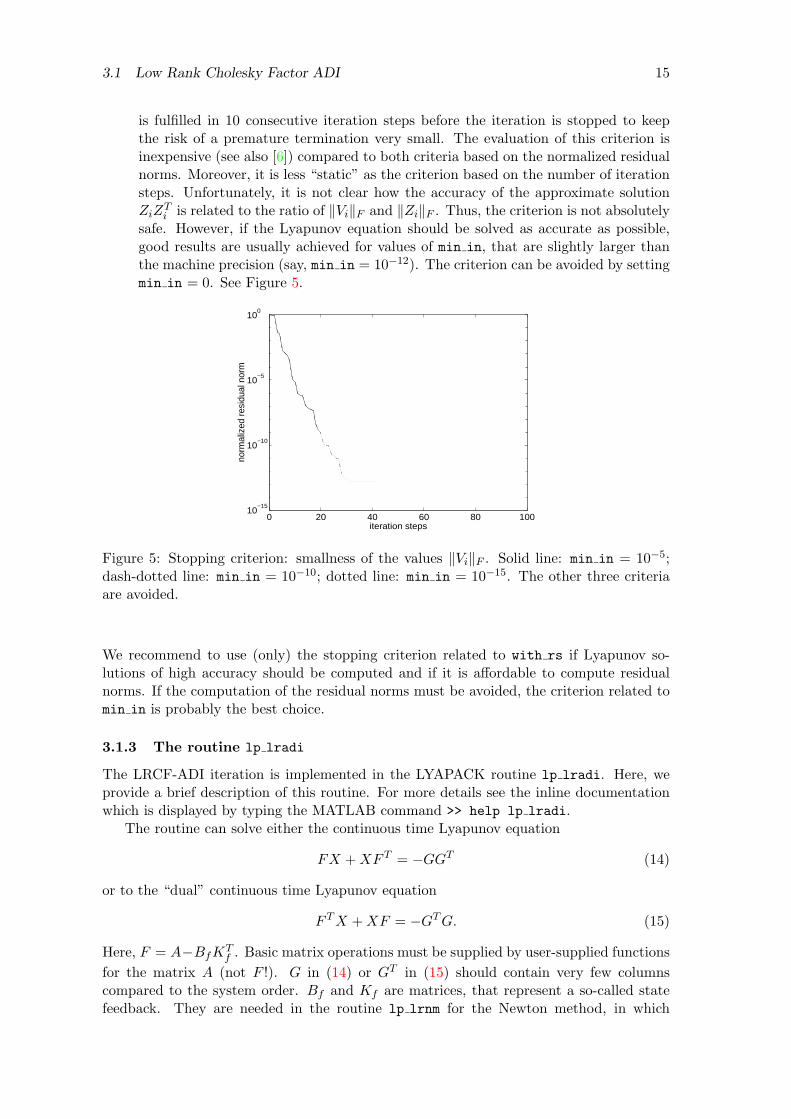
safe. However, if the Lyapunov equation should be solved as accurate as possible,good results are usually achieved for values of min in, that are slightly larger thanthe machine precision (say, min in = 10−12). The criterion can be avoided by settingmin in = 0. See Figure 5.
0 20 40 60 80 10010
−15
10−10
10−5
100
iteration steps
norm
aliz
ed r
esid
ual n
orm
Figure 5: Stopping criterion: smallness of the values ‖Vi‖F . Solid line: min in = 10−5;dash-dotted line: min in = 10−10; dotted line: min in = 10−15. The other three criteriaare avoided.
We recommend to use (only) the stopping criterion related to with rs if Lyapunov so-lutions of high accuracy should be computed and if it is affordable to compute residualnorms. If the computation of the residual norms must be avoided, the criterion related tomin in is probably the best choice.
3.1.3 The routine lp lradi
The LRCF-ADI iteration is implemented in the LYAPACK routine lp lradi. Here, weprovide a brief description of this routine. For more details see the inline documentationwhich is displayed by typing the MATLAB command >> help lp lradi.
The routine can solve either the continuous time Lyapunov equation
FX +XF T = −GGT (14)
or to the “dual” continuous time Lyapunov equation
F TX +XF = −GTG. (15)
Here, F = A−BfKTf . Basic matrix operations must be supplied by user-supplied functions
for the matrix A (not F !). G in (14) or GT in (15) should contain very few columnscompared to the system order. Bf and Kf are matrices, that represent a so-called statefeedback. They are needed in the routine lp lrnm for the Newton method, in which

16 3 LYAPUNOV EQUATIONS
lp lradi is invoked. In general, users will not use this option, which means Bf = Kf = 0.However, if this is not the case, the matrices Bf and Kf must contain very few columnsto guarantee the efficiency of the routine.
The approximate solution of either Lyapunov equation is given by the low rankCholesky factor Z, for which ZZH ≈ X. Z has typically fewer columns than rows. (Oth-erwise, this routine and LYAPACK itself are useless!) In general, Z can be a complexmatrix, but the product ZZH is real. lp lradi can perform an optional internal post-processing step, which guarantees that the delivered low rank Cholesky factor Z is real.More precisely, the complex low rank Cholesky factor delivered by the LRCF-ADI itera-tion is transformed into a real low rank Cholesky factor of the same size, such that bothlow rank Cholesky factor products are identical. However, doing this requires additionalcomputation. (This option is not related to the “real version” of LRCF-ADI described in[6].)
Furthermore, there exists an option for directly generating the product of the (approx-imate) solution with a matrix, i.e., Kout = ZZHKin is computed without forming the lowrank Cholesky factor Z. Here, Kin must contain only few columns. However, this optionshould not be used by the user. It is needed in the implicit version of the Newton method.If this mode is used, stopping criteria based on the residual cannot be applied.
Calling sequences:
Depending on the choice of the mode parameter zk, the following two calling sequencesexist. However, it is recommended to use only the first mode.
• zk = ’Z’:
[Z, flag, res, flp] = lp_lradi( tp, zk, rc, name, Bf, Kf, G, p, ...max_it, min_res, with_rs, min_in, info)
• zk = ’K’:
[K_out, flag, flp] = lp_lradi( tp, zk, rc, name, Bf, Kf, G, p, ...K_in, max_it, min_in, info)
Input parameters:
tp: Mode parameter, which is either ’B’ or ’C’. If tp = ’B’, CALE (14) is solved.Otherwise, CALE (15) is solved.
zk: Mode parameter, which is either ’Z’ or ’K’. If zk = ’Z’, the low rank Choleskyfactor Z is computed. Otherwise, Kout = ZZHKin is computed directly.
rc: Mode parameter, which is either ’R’ or ’C’. If rc = ’C’, the routine delivers alow rank Cholesky factor, which is not real when non-real shift parameters are used.Otherwise, the low rank Cholesky factor resulting from the LRCF-ADI iteration istransformed into a real low rank Cholesky factor Z, which describes the identicalapproximate solution ZZT . Z is returned instead of Z.
name: The basis name of the USFs that realize BMOs with A.
Bf: Feedback matrix Bf , which is not used explicitely in general. For Bf = 0, set Bf =[].

3.2 Computation of ADI shift parameters 17
Kf: Feedback matrix Kf , which is not used explicitely in general. For Kf = 0, set Kf =[].
G: The matrix G.
p: Vector containing the suitably ordered ADI shift parameters P = {p1, . . . , pl}, whichare delivered by the routine lp para. If the number l of distinct parameters issmaller than imax in Algorithm 1, shift parameters are used cyclically. That means,pl+1 = p1, pl+2 = p2, . . ., p2l = pl, p2l+1 = p1, . . .
K in: The matrix Kin, which is only used in the mode zk = ’K’.
max it: Stopping parameter. See §3.1.2.
min res: Stopping parameter. See §3.1.2.
with rs: Stopping parameter. See §3.1.2.
min in: Stopping parameter. See §3.1.2.
info: Parameter, which determines the “amount” of information that is provided astext and/or residual history plot. The following values are possible: info = 0 (noinformation), 1, 2, and 3 (most possible information)
Output parameters:
Z: The low rank Cholesky factor Z, which is complex if rc = ’C’ and p is not a realvector.
K out: The matrix Kout, which is only returned in the mode zk = ’K’.
flag: A flag, that shows by which stopping criterion (or stopping parameter) the iterationhas been stopped. Possible values are ’I’ (for max it), ’R’ (for min res), ’S’ (forwith rs), and ’N’ (for min in).
res: A vector containing the history of the normalized residual norms. res(1) = 1 andres(i+1) is the normalized residual norm w.r.t. the iteration step i. If the stoppingcriteria are chosen, so that the normalized residual norms need not be computed,res = [] is returned.
flp: A vector containing the history of the flops needed for the iteration. flp(1) = 0 andflp(i+ 1) is the number of flops required for the iteration steps 1 to i. flp displaysonly the number of flops required for the actual iteration. The numerical costs forinitializing and generating data by USFs, the computation of ADI shift parameters,and the computation of normalized residual norms are not included.
3.2 Computation of ADI shift parameters
3.2.1 Theory and algorithm
In this section, we briefly describe a practical algorithm to compute a set P = {p1, . . . , pl} ofsuboptimal shift parameters, which are needed in the LRCF-ADI iteration. This algorithm[37] is implemented in the routine lp para, whose output is an ordered set of l distinctshift parameters.

18 3 LYAPUNOV EQUATIONS
The determination of (sub)optimal ADI shift parameters is closely connected with arational minimax problem (e.g., [46, 49, 51]) related to the function
sP(t) =|(t− p1) · . . . · (t− pl)||(t+ p1) · . . . · (t+ pl)|
.
This minimax problem can be stated as the choice of P, such that
maxt∈σ(F )
sP(t)
is minimized. Unfortunately, the spectrum σ(F ) is not known in general and it cannot becomputed inexpensively if F is very large. Furthermore, even if the spectrum or bounds forthe spectrum are known, no algorithms are available to compute the optimal parameterspi.
Our algorithm for the computation of a set of suboptimal shift parameters is numer-ically inexpensive and heuristic. It is based on two ideas. First, we generate a discreteset, which “approximates” the spectrum. This is done by a pair of Arnoldi processes; e.g.,[19]. The first process w.r.t. F delivers k+ values that tend to approximate “outer” eigen-values, which are generally not close to the origin, well. The second process w.r.t. F−1 isused to get k− approximations of eigenvalues near the origin, whose consideration in theADI minimax problem is crucial. The eigenvalue approximations delivered by the Arnoldiprocesses are called Ritz values. Second, we choose a set of shift parameters, which is asubset of the set of Ritz values R. This is done by a heuristic, that delivers a suboptimalsolution for the resulting discrete optimization problem. Note that the order in which thisheuristic delivers the parameters is advantageous. Loosely speaking, the parameters areordered such that parameters, which are related to a strong reduction in the ADI error,are applied first. For more details about the parameter algorithm, see [37].
Algorithm 2 (Suboptimal ADI parameters)
INPUT: F , l0, k+, k−
OUTPUT: P = {p1, . . . , pl}, where l = l0 or l0 + 1
1. Choose b0 ∈ Rn at random.
2. Perform k+ steps of the Arnoldi process w.r.t. (F, b0) and compute the set of Ritz valuesR+.
3. Perform k− steps of the Arnoldi process w.r.t. (F−1, b0) and compute the set of Ritzvalues R−.
4. R = {ρ1, . . . , ρk++k−} := R+ ∪ (1/R−)
5. IF R 6⊂ C−, remove unstable elements from R and display a warning.
6. Detect i with maxt∈R s{ρi}(t) = minρ∈Rmaxt∈R s{ρ}(t) and initialize
P :={{ρi} : ρi real{ρi, ρi} : otherwise
.
WHILE card(P) < l0
7. Detect i with sP(ρi) = maxt∈R sP(t) and set
P :={P ∪ {ρi} : ρi realP ∪ {ρi, ρi} : otherwise
.
END WHILE

3.2 Computation of ADI shift parameters 19
Obviously, the output of this algorithm is a proper parameter set; see §3.1.1. The numberof shift parameters is either l0 or l0 + 1. Larger values of k+ and k− lead to betterapproximations of the spectrum, but increase also the computational cost, because k+
matrix-vector multiplications with F must be computed in the first Arnoldi algorithm andk− systems of linear equations with F must be solved in the second one. A typical choice ofthe triple (l0, k+, k−) is (20,50,25). For “tough” problems these values should be increased.For “easy” ones they can be decreased. Note that decreasing l0 will reduce the memorydemand if shifted SLEs are solved directly, because in this case the amount of the memoryneeded to store the matrix factors is proportional to l.
Steps 6 and 7 require that R is contained in C−. However, this can only be guaranteedif F + F T is negative definite and exact machine precision is used. If F is unstable, thanLYAPACK cannot be applied anyway, because the ADI iteration diverges or, at least,stagnates. Experience shows that also in the case, when F is stable but F + F T is notdefinite, the Ritz values tend to be contained in the left half of the complex plane. Ifthis is not the case, unstable Ritz values are removed in Step 5, which is more or lessa not very elegant emergency measure. If LRCF-ADI run with the resulting parametersdiverges despite this measure, the matrix F is most likely unstable. In connection withthe LRCF-NM or LRCF-NM-I applied to ill-conditioned CAREs, this might be caused byround-off errors. There the so-called closed-loop matrix A − BfKT
f can be proved to bestable (in exact arithmetics), but the closed-loop poles (i.e, the eigenvalues of A−BfKT
f )can be extremely sensitive to perturbations, so that stability is not guaranteed in practice.
Figure 6 shows the result of the parameter algorithm for a random example of ordern = 500. The triple (l0, k+, k−) is chosen as (20,50,25). 21 shift parameters were returned.The picture shows the eigenvalues of F , the set R of Ritz values, and the set P of shiftparameters. Note that the majority of the shift parameters is close to the imaginary axis.
−2000 −1500 −1000 −500 0−500
−400
−300
−200
−100
0
100
200
300
400
500
real axis
imag
inar
y ax
is
Figure 6: Results of Algorithm 2. ×: eigenvalues of F ; ©: elements of R; ∗: elements ofP ⊂ R.

20 3 LYAPUNOV EQUATIONS
3.2.2 The routine lp para
Calling sequences:
The following two calling sequences are possible:
[p,err_code,rw,Hp,Hm] = lp_para(name,Bf,Kf,l0,kp,km)
[p,err_code,rw,Hp,Hm] = lp_para(name,Bf,Kf,l0,kp,km,b0)
However, usually one is only interested in the first output parameter p.
Input parameters:
name: The basis name of the USFs that realize BMOs with A.
Bf: Feedback matrix Bf , which is not used explicitely in general. For Bf = 0, set Bf =[].
Kf: Feedback matrix Kf , which is not used explicitely in general. For Kf = 0, set Kf =[].
l0: Parameter l0. Note that k+ + k− > 2l0 is required.
kp: Parameter k+.
km: Parameter k−.
b0: This optional argument is an n-vector, that is used as starting vector in both Arnoldiprocesses. If b0 is not provided, this vector is chosen at random, which means thatdifferent results can be returned by lp para in two different runs with identical inputparameters.
Output parameters:
p: A vector containing the ADI shift parameters P = {p1, . . . , pl}, where either l = l0 orl = l0 + 1. It is recommended to apply the shift parameters in the same order in theroutine lp lradi as they are returned by this routine.
err code: This parameter is an error flag, which is either 0 or 1. If err code = 1, theroutine encountered Ritz values in the right half of the complex plane, which areremoved in Step 5 of Algorithm 2. err code = 0 is the standard return value.
rw: A vector containing the Ritz value set R.
Hp: The Hessenberg matrix produced by the Arnoldi process w.r.t. F .
Hm: The Hessenberg matrix produced by the Arnoldi process w.r.t. F−1.
3.3 Case studies
See §C.2.1.

21
4 Model reduction
4.1 Preliminaries
Roughly speaking, model reduction is the approximation of the dynamical system
x(τ) = Ax(τ) +Bu(τ)
y(τ) = Cx(τ)(16)
with A ∈ Rn,n, B ∈ Rn,m, and C ∈ Rq,n by a reduced system
˙x(τ) = Ax(τ) + Bu(τ)
y(τ) = Cx(τ)(17)
with A ∈ Rk,k, B ∈ Rk,m, C ∈ Rq,k (or, possibly, A ∈ Ck,k, B ∈ Ck,m, C ∈ Cq,k), andk < n. In particular, we consider the case where the system order n is large, and m andq are much smaller than n. Furthermore, we assume that A is stable. Several ways existto evaluate the approximation error between the original system and the reduced system.Frequently, the difference between the systems (16) and (17) measured in the L∞ norm
‖G− G‖L∞ = supω∈R‖G(ω)− G(ω)‖ (18)
is used to do this, where =√−1 and ‖ · ‖ is the spectral norm of a matrix. Moreover,
G and G are the transfer functions of the systems (16) and (17), which are defined asG(s) = C(sIn −A)−1B and G(s) = C(sIk − A)−1B.
LYAPACK contains implementations of two algorithms (LRSRM and DSPMR) forcomputing reduced systems. Both model reduction algorithms belong to the class of statespace projection methods, where the reduced system is given as
A = SHC ASB, B = SHC B, C = CSB. (19)
Here, SB, SC ∈ Cn,k are certain projection matrices, which fulfill the biorthogonality con-dition
SHC SB = Ik.
Furthermore, both model reduction algorithms rely on low rank approximations to thesolutions (Gramians) of the continuous time Lyapunov equations
AXB +XBAT = −BBT (20)
ATXC +XCA = −CTC. (21)
This means that we assume that low rank Cholesky factors ZB ∈ Cn,rB and ZC ∈ Cn,rCwith rB, rC << n are available, such that ZBZHB ≈ XB and ZCZ
HC ≈ XC . In LYAPACK
these low rank Cholesky factors are computed by the LRCF-ADI iteration; see §3.1. In§§4.2 and 4.3 we will briefly describe the two model reduction algorithms LRSRM [39, 33]and DSPMR [32, 39]. In [39] a third method called LRSM (low rank Schur method)is proposed. However, this less efficient method is not implemented in LYAPACK. Thedistinct merit of LRSRM and DSPMR compared to standard model reduction algorithms,such as standard balanced truncation methods [47, 44, 48] or all-optimal Hankel normapproximation [18]), is their low numerical cost w.r.t. both memory and computation. Onthe other hand, unlike some standard methods, the algorithms implemented in LYAPACKdo generally not guarantee the stability of the reduced system. If stability is crucial, this
22 4 MODEL REDUCTION
property must be checked numerically after running LRSRM or DSPMR. If the reducedsystem is not stable, several measures can be tried. For example, one can simply remove theunstable modes by modal truncation [11]. Another option is to run LRSRM or DSPMRagain using more accurate low rank Cholesky factors ZB and ZC . Note that for someproblems the error function ‖G(ω) − G(ω)‖ in ω, which characterizes the frequencyresponse of the difference of both systems, can be evaluated by supplementary LYAPACKroutines; see §6.
If the low rank Cholesky factors ZB and ZC delivered by the LRCF-ADI iterationare not real, then the reduced systems are not guaranteed to be real. This problemis discussed more detailed in [33] for the low rank square root method. If the reducedsystem needs to be real, it is recommended to check a posteriori whether the result of lowrank square root method or dominant subspace projection model reduction is real. It ispossible to transform a reduced complex system into a real one by a unitary equivalencetransformation; see [33]. A much simpler way, of course, is using the option rc = ’R’for which the routine lp lradi delivers real low rank Cholesky factors (at the price of asomewhat increased numerical cost).
4.2 Low rank square root method
4.2.1 Theory and algorithm
The low rank square root method (This algorithm is named SLA in [33].) (LRSRM) [39, 33]is only a slight modification of the classical square root method [47], which in turn is anumerically advantageous version of the balanced truncation technique [35]. The followingalgorithm is implemented in the LYAPACK routine lp lrsrm:
Algorithm 3 (Low rank square root method (LRSRM))
INPUT: A, B, C, ZB, ZC , k
OUTPUT: A, B, C
1. UCΣUHB := ZHC ZB (“thin” SVD with descending ordered singular values)
2. SB = ZBUB (:,1:k)Σ−1/2(1:k,1:k), SC = ZCUC (:,1:k)Σ
−1/2(1:k,1:k)
3. A = SHC ASB, B = SHC B, C = CSB
The only difference between the classical square root method and this algorithm is, thathere (approximate) low rank Cholesky factors ZB and ZC are used instead of exactCholesky factors of the Gramians, which have possibly full rank. This reduces in par-ticular the numerical cost for the singular value decomposition in Step 1 considerably.
However, there are two basic drawbacks of LRSRM compared to the “exact” squareroot method. Unlike LRSRM, the latter delivers stable reduced systems under mild condi-tions. Furthermore, there exists an upper error bound for (18) for the standard square rootmethod, which does not apply to the low rank square root method. Thus, it is not surpris-ing that the performance of Algorithm 3 depends on the accuracy of the approximate lowrank Cholesky factor products ZBZHB and ZCZHC and the value k, where k ≤ rankZHC ZB.This makes the choice of the quantities rB, rC , and k a trade-off. Large values of rB andrC , and values of k much smaller than rankZHC ZB tend to keep the deviation of the lowrank square root method from the standard square root method small. On the other handthe computational efficiency of the low rank square roo method is decreased in this way.However, LRCF-ADI often delivers low rank Cholesky factors ZB and ZC , whose products
4.2 Low rank square root method 23
approximate the system Gramians nearly up to machine precision. In this case the re-sults of the LYAPACK implementation of the low rank square root method will be aboutas good as those by any standard implementation of the balanced truncation technique,which, however, can be still numerically much more expensive.
Finally, note that the classical square root method is well-suited to compute (nu-merically) minimal realizations; e.g., [48]. LRSRM (as well as DSPMR) can be used tocompute such realizations for large systems. The term “numerically minimal realization”is not well-defined. Loosely speaking, it is rather the concept of computing a reducedsystem, for which the (relative) approximation error (18) is of magnitude of the machineprecision. See Figure 14 in §C.3.3.
4.2.2 Choice of reduced order
In the LYAPACK implementation of the low rank square root method, the reduced or-der k can be chosen a priori or in dependence of the descending ordered singular valuesσ1, σ2, . . . , σr computed in Step 1, where r = rankZHC ZB.
• Maximal reduced order. The input parameters max ord of the routine lp lrsrmprescribes the maximal admissible value for the reduced order k, i.e., k ≤ max ord isrequired. If the choice of this value should be avoided, one can set max ord = n ormax ord = [].
• Maximal ratio σk/σ1. The input parameter tol prescribes the maximal admissiblevalue for the ratio σk/σ1. That means k is chosen as the largest index for whichσk/σ1 ≥ tol. This means that one will generally choose a value of tol between themachine precision an 1.
In general, both parameters will determine different values of k. The routine lp lrsrmuses the smaller value.
4.2.3 The routine lp lrsrm
Algorithm LRSRM is implemented in the LYAPACK routine lp lrsrm. We provide abrief description of this routine. For more details see the inline documentation which isdisplayed by typing the MATLAB command >> help lp lrsrm.
Calling sequence:
[Ar ,Br, Cr, SB, SC, sigma] = lp_lrsrm( name, B, C, ZB, ZC, ...max_ord, tol)
Input parameters:
name: The basis name of the user supplied functions that realize basic matrix operationswith A.
B: System matrix B.
C: System matrix C.
ZB: LRCF ZB ∈ Cn,rB . This routine is only efficient if rB << n.
ZC: LRCF ZC ∈ Cn,rC . This routine is only efficient if rC << n.

24 4 MODEL REDUCTION
max ord: A parameter for the choice of the reduced order k; see §4.2.2.
tol: A parameter for the choice of the reduced order k; see §4.2.2.
Output parameters:
Ar: Matrix A ∈ Ck,k of reduced system.
Br: Matrix B ∈ Ck,m of reduced system.
Cr: Matrix C ∈ Cq,k of reduced system.
SB: Projection matrix SB.
SC: Projection matrix SC .
sigma: Vector containing the singular values computed in Step 1.
Usually, one is only interested in the first three output parameters.
4.2.4 Case studies
See §C.3.
4.3 Dominant subspaces projection model reduction
4.3.1 Theory and algorithms
The dominant subspaces projection model reduction (DSPMR) [32, 39], which is providedas LYAPACK routine lp dspmr, is more heuristic in nature. The basic idea behind thismethod is that the input-state behavior and the state-output behavior of the system (16)tend to be dominated by states, which have a strong component w.r.t. the dominantinvariant subspaces of the Gramians XB and XC . These dominant invariant subspaces areapproximated by the left singular vectors of ZB and ZC provided that XB ≈ ZBZ
HB and
XC ≈ ZCZHC . The motivation of the dominant subspace correction method is discussed
at length in [39]. Compared to the low rank square root method, the approximationproperties of the reduced systems by DSPMR are often less satisfactory, i.e., the errorfunction ‖G(s) − G(s)‖ tends to be less small. On the other hand, DSPMR sometimesdelivers a stable reduced system, when that by LRSRM is not stable. In DSPMR, thestability of the reduced system is guaranteed at least if A+AT is negative definite. Note alsothat DSPMR uses an orthoprojection, whereas LRSRM is based on an oblique projection.For this reason, DSPMR is also advantageous w.r.t. preserving passivity.
Algorithm 4 (Dominant subspaces projection model reduction (DSPMR))
INPUT: A, B, C, ZB, ZC , k
OUTPUT: A, B, C
1. Z =[
1||ZB ||F
ZB1
||ZC ||FZC
]2. UΣV H := Z (“thin” SVD with descending ordered singular values)
3. S = U(:,1:k)
4. A = SHAS, B = SHB, C = CS

4.3 Dominant subspaces projection model reduction 25
4.3.2 Choice of reduced order
In the LYAPACK implementation of DSPMR, the reduced order k can be chosen a priorior in dependence of the descending ordered singular values σ1, σ2, . . . , σr computed in Step2, where r = rankZ.
• Maximal reduced order. The input parameter max ord of the routine lp dspmrprescribes the maximal admissible value for the reduced order k, i.e., k ≤ max ord isrequired. To avoid this choice, one can set max ord = n or max ord = [].
• Maximal ratio σk/σ1. The input parameter tol determines the maximal admissiblevalue for the ratio σk/σ1. More precisely, k is chosen as the largest index for whichσk/σ1 ≥
√tol. Note that here the square root of tol is used in contrast to LRSRM.
(Note that the values σi have somewhat different meanings in LRSRM and DSPMR.)
In general, both parameters will determine different values of k. The routine lp dspmruses the smaller value. Finally, it should be mentioned, that, at least in exact arithmetics,both LRSRM and DSPMR (run with identical values max ord and tol) deliver the sameresult for state-space symmetric systems (i.e., systems, where A = AT and C = BT ).
4.3.3 The routine lp dspmr
Algorithm DSPMR is implemented in the LYAPACK routine lp dspmr. We provide abrief description of this routine. For more details see the inline documentation which isdisplayed by typing the MATLAB command >> help lp dspmr.
Calling sequence:
[Ar ,Br, Cr, S] = lp_dspmr( name, B, C, ZB, ZC, max_ord, tol)
Input parameters:
name: The basis name of the user supplied functions that realize basic matrix operationswith A.
B: System matrix B.
C: System matrix C.
ZB: LRCF ZB ∈ Cn,rB . This routine is only efficient if rB << n.
ZC: LRCF ZC ∈ Cn,rC . This routine is only efficient if rC << n.
max ord: A parameter for the choice of the reduced order k; see §4.3.2.
tol: A parameter for the choice of the reduced order k; see §4.3.2.
Output parameters:
Ar: Matrix A ∈ Ck,k of reduced system.
Br: Matrix B ∈ Ck,m of reduced system.
Cr: Matrix C ∈ Cq,k of reduced system.
S: Projection matrix S.

26 5 RICCATI EQUATIONS
4.3.4 Case studies
See §C.3.
5 Riccati equations and linear-quadratic optimal controlproblems
5.1 Preliminaries
This section mainly deals with the efficient numerical solution of continuous time algebraicRiccati equations of the type
CTQC +ATX +XA−XBR−1BTX = 0, (22)
where A ∈ Rn,n, B ∈ Rn,m, and C ∈ Rq,n with m, q << n. Moreover, we assume thatQ ∈ Rq,q is symmetric, positive semidefinite and R ∈ Rm,m is symmetric, positive definite.Unlike in the other sections of this document, we do not assume here that A is stable, butit is required that a matrix K(0) is given, such that A− BK(0)T is stable. Such a matrixK(0) can be computed by partial pole placement algorithms [21], for example.
In general, the solution of (22) is not unique. However, under the above assumptions, aunique, stabilizing solution X exists, which is the solution of interest in most applications;e.g., [34, 29]. A solution X is called stabilizing if the closed-loop matrix A−BR−1BTX isstable.
Algebraic Riccati equations arise from numerous problems in control theory, such asrobust control or certain balancing and model reduction techniques for unstable systems.Another application, for which algorithms are provided by LYAPACK, is the solutionof the linear quadratic optimal control problem. In this paragraph, we briefly describethe connection between linear quadratic optimal control problems and algebraic Riccatiequations. The linear quadratic optimal control problem is a constrained optimizationproblem. The cost functional to be minimized, is
J (u, y, x0) =12
∫ ∞0
y(τ)TQy(τ) + u(τ)TRu(τ)dτ , (23)
where Q = QT ≥ 0 and R = RT > 0. The constraints are given by the dynamical system
x(τ) = Ax(τ) +Bu(τ)
y(τ) = Cx(τ)(24)
and the initial conditionx(0) = x0. (25)
The solution of this optimization problem is described by the feedback matrix K, that isdefined as
K = XBR−1, (26)
where X is the stabilizing solution of the algebraic Riccati equation (22). The correspond-ing control function is given by the state-feedback
u(τ) = −KTx(τ)
and the initial condition (25).

5.2 Low rank Cholesky factor Newton method 27
To sum up, we consider two problems in this section. The first one is the numericalcomputation of the stabilizing solution of the continuous time algebraic Riccati equations(22). The second problem is the solution of the linear quadratic optimal control problem(23,24,25), which is a particular application of algebraic Riccati equations. Its solutioncan be described by the stabilizing solution X, from which the optimal state-feedback caneasily be computed via (26), or by the feedback K itself.
LYAPACK contains implementations of the low rank Cholesky factor Newton method(LRCF-NM) and the implicit low rank Cholesky factor Newton method (LRCF-NM-I) pro-posed in [6]. LRCF-NM delivers a LRCF Z, such that the product ZZH approximates theRiccati solution X. This means that LRCF-NM can be used to solve both continuous timealgebraic Riccati equations and linear quadratic optimal control problems. The implicitversion LRCF-NM-I, which directly computes an approximation to K without forming Zor X, can only be used to solve the linear quadratic optimal control problem in a morememory efficient way.
Both LRCF-NM and LRCF-NM-I are modifications of the classical Newton methodfor algebraic Riccati equations [28], or more precisely, combinations of the Newton methodwith the LRCF-ADI iteration. We will describe these combinations in §§5.2 and 5.3. Theclassical formulation of the Newton method is given by the double step iteration
Solve Lyapunov equation(AT −K(k−1)BT )X(k) +X(k)(A−BK(k−1)T ) = −CTQC −K(k−1)RK(k−1)T
for X(k),
K(k) = X(k)BR−1
(27)
for k = 1, 2, 3, . . ., which generates a sequence of iterates X(k). This sequence convergestowards the stabilizing solution X if the initial feedback K0 is stabilizing, i.e., A−BK(0)T
is stable. Then, the convergence is global and quadratic.
5.2 Low rank Cholesky factor Newton method
Due to the symmetry and definiteness assumptions, the matrices Q and R can be factored(by a Cholesky factorization, for example) as
Q = QQT and R = RRT , (28)
where the matrices Q ∈ Rq,h (h ≤ q) and R ∈ Rm,m have full rank. Thus, the Lyapunovequations to be solved in (27) have the structure
F (k)X(k) +X(k)F (k)T = −G(k)G(k)T
where F (k) = AT − K(k−1)BT and G(k) =[CT Q K(k−1)R
]. Note that G(k) contains
only t = m + h << n columns. Hence, these Lyapunov can be solved efficiently by theLRCF-ADI iteration. The Lyapunov solutions form a sequence of approximate solutionsto the algebraic Riccati equations (22). Therefore, the inclusion of Algorithm 1 into theNewton iteration (27) can be utilized to determine low rank Cholesky factor products whichapproximate the solution of the algebraic Riccati equation (22). The resulting algorithmlow rank Cholesky factor Newton method is described below.
Algorithm 5 (Low rank Cholesky factor Newton method (LRCF-NM))

28 5 RICCATI EQUATIONS
INPUT: A, B, C, Q, R, K(0) for which A−BK(0)T is stable (e.g., K(0) = 0 if A is stable)
OUTPUT: Z = Z(kmax), such that ZZH approximates the solution X of the algebraicRiccati equation (8)
FOR k = 1, 2, . . . , kmax
1. Determine (sub)optimal ADI shift parameters p(k)1 , p
(k)2 , . . . with respect to the
matrix F (k) = AT −K(k−1)BT .
2. G(k) =[CT Q K(k−1)R
]3. Compute matrix Z(k) by Algorithm 1, such that the low rank Cholesky factor
product Z(k)Z(k)H
approximates the solution of F (k)X(k) +X(k)F (k)T = −G(k)G(k)T .
4. K(k) = Z(k)(Z(k)HBR−1)
END
Similar to the LRCF-ADI iteration for the solution of Lyapunov equations, the distinctmerit of this algorithm is that the (approximate) solution of the algebraic Riccati equationsis provided as a low rank Cholesky factor product rather than an explicit dense matrix. Inparticular, this allows the application of the algorithm to problems of large order n, wheredense n×n matrices cannot be stored in the computer memory. Moreover, the LRCF-NMrequires often much less computation compared to the standard implementation, whereLyapunov are solved directly by the Bartels-Stewart or the Hammarling method; see §7.See [6] for more technical details of the LRCF-NM.
5.3 Implicit low rank Cholesky factor Newton method
The idea behind the implicit version of LRCF-NM is that the solution of the linearquadratic optimal control problem is described by the state feedback matrix K, whichgenerally contains much less columns than the low rank Cholesky factor Z delivered byLRCF-NM or even the exact solution X. LRCF-NM-I is mathematically equivalent toLRCF-NM. It computes an approximation to K without forming LRCF-NM iterates Z(k)
and LRCF-ADI iterates Z(k)i at all. The trick is to generate the matrix K(k) itself in Step
3 of Algorithm 5 instead of solving the Lyapunov equation for Z(k) and computing theproduct K(k) = Z(k)Z(k)HBR−1 in Step 4. Note that the matrix K(k) can be accumulatedin the course of the “inner” LRCF-ADI iteration as
K(k) = limi→∞
K(k)i ,
where
K(k)i := Z
(k)i Z
(k)i
HBR−1 =
i∑j=1
V(k)j
(V
(k)j
HBR−1
). (29)
This means, that the (exact) matrix K is the limit of the matrices K(k)i for k, i→∞. This
consideration motivates the following Algorithm 6, which is best understood as a versionof the LRCF-NM with an inner loop (Steps 4 and 5) consisting of interlaced sequencesbased on Step 3 in Algorithm 1 and the partial sums given by the right hand term in (29).
Algorithm 6 (Implicit low rank Cholesky factor Newton method (LRCF-NM-I))

5.4 Stopping criteria 29
INPUT: A, B, C, Q, R, K(0) for which A−BK(0)T is stable (e.g., K(0) = 0, if A is stable)
OUTPUT: K(kmax), which approximates K given by (26)
FOR k = 1, 2, . . . , kmax
1. Determine (sub)optimal ADI shift parameters p(k)1 , p
(k)2 , . . . with respect to the
matrix F (k) = AT −K(k−1)BT .
2. G(k) =[CT Q K(k−1)R
]3. V (k)
1 =√−2 Re p(k)
1 (F (k) + p(k)1 In)−1G(k)
FOR i = 2, 3, . . . , i(k)max
4. V (k)i =
√Re p(k)
i /Re p(k)i−1
(V
(k)i−1 − (p(k)
i + p(k)i−1)(F (k) + p
(k)i In)−1V
(k)i−1
)5. K(k)
i = K(k)i−1 + V
(k)i
(V
(k)i
HBR−1
)END
6. K(k) = K(k)
i(k)max
END
Again, see [6] for more implementational details.
5.4 Stopping criteria
As far as possible, the same stopping criteria are used in LRCF-NM and LRCF-NM-I forterminating the (outer) Newton iteration. The LYAPACK routine lp lrnm, in which bothmethods are implemented, offers the following five criteria:
• maximal number of iteration steps: used in LRCF-NM and LRCF-NM-I;
• tolerance for the normalized residual norm: used in LRCF-NM only;
• stagnation of the normalized residual norm (most likely caused by round-off errors):used in LRCF-NM only;
• smallness of the relative change of the feedback matrix (RCF): Used in LRCF-NMand LRCF-NM-I;
• stagnation of the relative change of the feedback matrix: used in LRCF-NM andLRCF-NM-I.
Here, the normalized residual norm corresponding to the low rank Cholesky factor Z(k) isdefined as
NRN(Z(k)) =‖CTQC +ATZ(k)Z(k)H + Z(k)Z(k)HA− Z(k)Z(k)HBR−1BTZ(k)Z(k)H‖F
‖CTQC‖F,
(30)whereas the relative change of the feedback matrix related to the matrices K(k−1) andK(k) is
RCF(K(k−1),K(k)) =‖K(k) −K(k−1)‖F
‖K(k)‖F. (31)

30 5 RICCATI EQUATIONS
Many of the remarks on stopping criteria for the LRCF-ADI iteration made in §3.1.2 alsoapply to stopping criteria for LRCF-NM or LRCF-NM-I. In particular, the application ofstopping criteria, which require the computation of normalized residual norms is numer-ically expensive. Although the applied computational method [6] exploits the low rankstructure of the approximate solutions, it can be more expensive than the iteration itself.Moreover, it is not possible to use residual based stopping criteria for LRCF-NM-I, becausethere the low rank Cholesky factors Z(k) are not formed at all, which is the only reasonwhy one would apply LRCF-NM-I instead of LRCF-NM.
The consideration of (31) for the construction of heuristic stopping criteria is relatedto the fact that in some sense the matrices K(k) rather than the low rank Cholesky factorsZ(k) or their products are the quantities of interest when the optimal control problemshould be solved. However, stopping criteria related to K(k) are somewhat dubious whenthe optimal feedback K or, more precisely, the product BKT is very small compared to A,because then small relative changes in K hardly change the closed-loop matrix A−BKT .On the other hand, the accuracy of K does not play a crucial role in such situations, whichmeans that a possibly premature termination of the Newton iteration would not be veryharmful.
We will now discuss the five stopping criteria. Convergence plots generated for anexample problem illustrate their effects. Note that, similar to the criteria for the LRCF-ADI iteration described in §3.1.2, the following stopping criteria can be “activated” or“avoided”.
• Stopping criterion: maximal number of iteration steps. This criterion isrepresented by the input parameter max it r in the routine lp lrnm. The iterationis stopped by this criterion after max it r iterations steps. This criterion can beavoided by setting max it r = +Inf (i.e., max it r =∞). Obviously, no additionalcomputations need to be performed to evaluate it. The drawback of this stopping cri-terion is, that it is not directly related to the attainable accuracy. This is illustratedby Figure 7.
0 5 10 15 20
10−15
10−10
10−5
100
iteration steps
norm
aliz
ed r
esid
ual n
orm
Figure 7: Stopping criterion: maximal number of iteration steps. Solid line: max it r = 5;dash-dotted line: max it r = 10; dotted line: max it r = 20. The other four criteria areavoided.
• Stopping criterion: tolerance for the normalized residual norm. This cri-terion is represented by the input parameter min res r in the routine lp lrnm. The

5.4 Stopping criteria 31
iteration is stopped by this criterion as soon as
NRN(Z(k)) ≤ min res r.
This criterion can be avoided by setting min res r = 0. (Because of round-off errorsit is practically impossible to attain NRN(Z(k)) = 0.) It requires the computation ofnormalized residual norms and is computationally expensive. A further drawback ofthis criterion is that it will either stop the iteration before the maximal accuracy isattained (see min res r = 10−5, 10−10 in Figure 8) or it will not stop the iterationat all (see min res r = 10−15 in Figure 8). If you want to avoid this criterion, butcompute the convergence history provided by the output vector res r, set min res rto a value much smaller than the machine precision (say, min res r = 10−100).
0 5 10 15 20
10−15
10−10
10−5
100
iteration steps
norm
aliz
ed r
esid
ual n
orm
Figure 8: Stopping criterion: tolerance for the normalized residual norm. Solid line:min res r = 10−5; dash-dotted line: min res r = 10−10; dotted line: min res r = 10−15.Here, the dash-dotted and the solid line are identical. The other four criteria are avoided.
• Stopping criterion: stagnation of the normalized residual norm. This cri-terion is represented by the input parameter with rs r in the routine lp lrnm. Itis activated if with rs r = ’S’ and avoided if with rs r = ’N’. The iteration isstopped by this criterion when a stagnation of the normalized residual norm curve isdetected. In contrast to the corresponding criterion for the LRCF-ADI iteration, thiscriterion stops the iteration, when the stagnation of the normalized residual norm isdetected for a single iteration step. Of course, this is a slightly heuristic criterion butit works very well in practice. It requires the computation of the normalized residualnorm and is computationally expensive. See Figure 9.
• Stopping criterion: smallness of the the relative change of the feedbackmatrix. This criterion is represented by the input parameter min ck r in the routinelp lrnm. The iteration is stopped by this criterion as soon as
RCF(K(k−1),K(k)) ≤ min ck r.
This criterion can be avoided by setting min ck r = 0. It is numerically very inex-pensive. On the other hand it is heuristic and not directly related to the accuracyin Z(k). See Figure 10.

32 5 RICCATI EQUATIONS
0 5 10 15 20
10−15
10−10
10−5
100
iteration steps
norm
aliz
ed r
esid
ual n
orm
Figure 9: Stopping criterion: Stagnation of the normalized residual norms. Solid line:with rs r = ’S’; dotted line: with rs r = ’N’. The other four criteria are avoided.
• Stopping criterion: stagnation of the relative change of the feedback ma-trix. This criterion is represented by the input parameter with ks r in the routinelp lrnm. It is activated if with ks r = ’L’ and avoided if with ks r = ’N’. Theiteration is stopped by this criterion when a stagnation of the relative change of thefeedback matrix is detected. Similar to the last criterion, this is a inexpensive, butheuristic stopping criterion. See Figure 11.
We recommend to use (only) the stopping criterion related to with rs r if algebraic Riccatiequations solutions of high accuracy should be computed and if it is affordable to computenormalized residual norms. If the computation of the normalized residual norms must beavoided, the combination of the criteria related to min ck r and with rs r is probably thebest choice. Experience shows that often only one of them will stop the iteration after areasonable number of steps. See, for example, Figure 11, where the criterion related towith rs r failed.
5.5 The routine lp lrnm
Both LRCF-NM and LRCF-NM-I are implemented in the LYAPACK routine lp lrnm. Weprovide a brief description of this routine. For more details see the inline documentationwhich is displayed by typing the MATLAB command >> help lp lrnm.
The approximate solution of the algebraic Riccati equations (22) is given by the lowrank Cholesky factor Z, such that ZZH ≈ X. Z has typically fewer columns than rows.Otherwise, LRCF-NM is useless! In general, Z can be a complex matrix, but the productZZH is real. In the explicit mode of lp lrnm (i.e., the one for LRCF-NM) an optionalinternal postprocessing step can be performed, which guarantees that the delivered lowrank Cholesky factor Z is real. This requires additional computation. This postprocessingis only done for the low rank Cholesky factor computed in the last Newton step. Thismeans, that its relative contribution to the overall cost is smaller than in the LRCF-ADIiteration.
Calling sequences:
Depending on the choice of the mode parameter zk, the following two calling sequencesexist. For zk = ’Z’, the low rank Cholesky factor Z is computed by LRCF-NM, whereas

5.5 The routine lp lrnm 33
0 5 10 15 20
10−15
10−10
10−5
100
iteration steps
norm
aliz
ed r
esid
ual n
orm
Figure 10: Stopping criterion: Smallness of the the relative change of the feedback matrix.Solid line: min ck r = 10−4; dash-dotted line: min ck r = 10−8; dotted line: min ck r= 10−16. The other four criteria are avoided. Note that it is mere coincidence, thatmin ck r = 10−8 (dash-dotted line) leads to the termination after the “optimal” numberof steps.
for zk = ’K’, the feedback matrix K is computed by LRCF-NM-I.
• zk = ’Z’:
[Z, flag_r, res_r, flp_r, flag_l, its_l, res_l, flp_l] = ...lp_lrnm( zk, rc, name, B, C, Q0, R0, K_in, max_it_r, ...min_res_r, with_rs_r, min_ck_r, with_ks_r, info_r, kp, km, ...l0, max_it_l, min_res_l, with_rs_l, min_in_l, info_l )
• zk = ’K’:
[K_out, flag_r, flp_r, flag_l, its_l, flp_l] = lp_lrnm(...zk, name, B, C, Q0, R0, K_in, max_it_r, min_ck_r, ...with_ks_r, info_r, kp, km, l0, max_it_l, min_in_l, info_l )
Input parameters:
zk: Mode parameter, which is either ’Z’ or ’K’. If zk = ’Z’, the low rank Cholesky factorZ = Z(kmax) is computed by LRCF-NM. Otherwise, K(kmax) is directly computed byLRCF-ADI-I.
rc: Mode parameter, which is either ’R’ or ’C’. If rc = ’C’, the routine delivers a lowrank Cholesky factor, which is not real when non-real shift parameters are used inthe last Newton step. Otherwise, this possibly complex low rank Cholesky factoris transformed into a real low rank Cholesky factor Z, which describes the identi-cal approximate solution ZZT . Z is returned instead of Z. The parameter rc isnot needed in the mode for LRCF-NM-I, because the returned feedback (parameterK out) is always real, provided that K(0) (parameter K in) is real.
name: The basis name of the user supplied functions that realize basic matrix operationswith A.
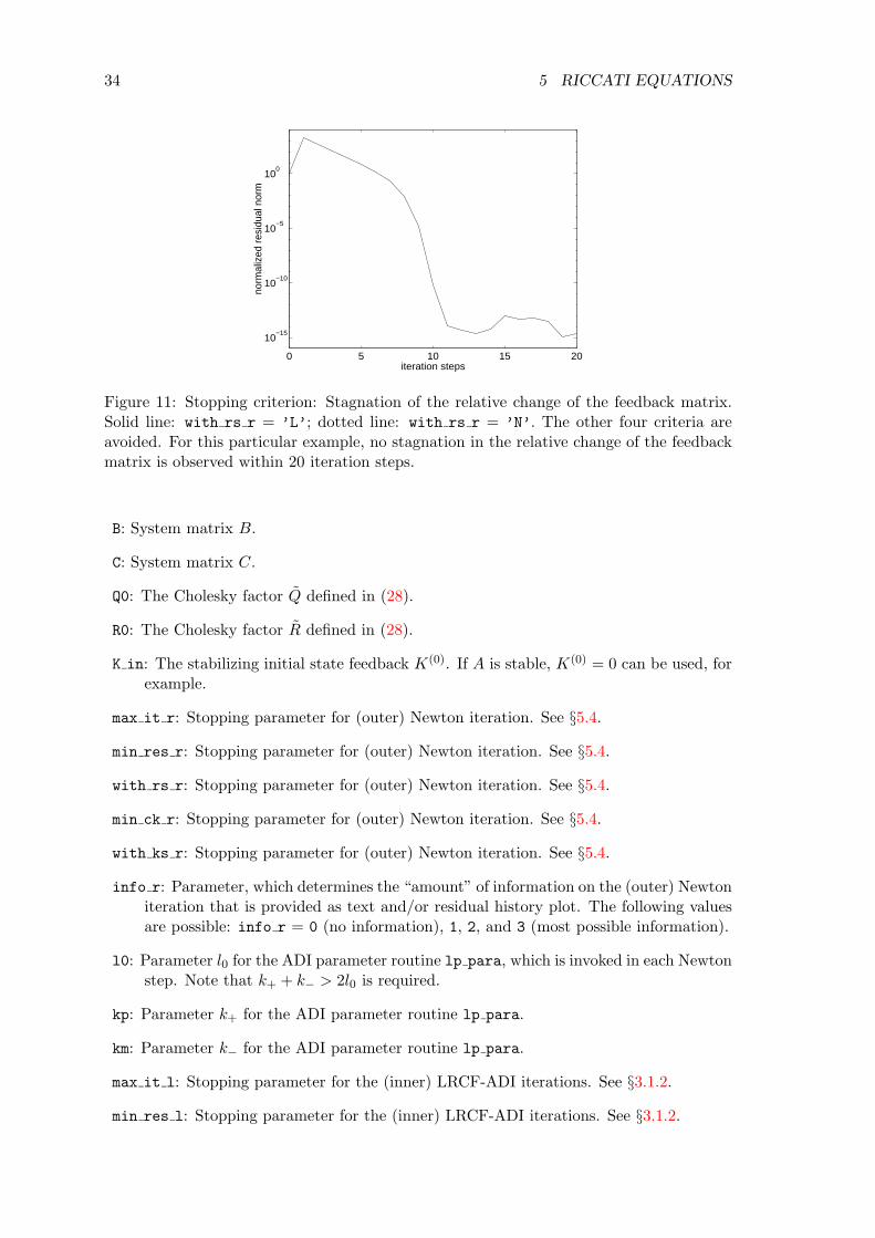
34 5 RICCATI EQUATIONS
0 5 10 15 20
10−15
10−10
10−5
100
iteration steps
norm
aliz
ed r
esid
ual n
orm
Figure 11: Stopping criterion: Stagnation of the relative change of the feedback matrix.Solid line: with rs r = ’L’; dotted line: with rs r = ’N’. The other four criteria areavoided. For this particular example, no stagnation in the relative change of the feedbackmatrix is observed within 20 iteration steps.
B: System matrix B.
C: System matrix C.
Q0: The Cholesky factor Q defined in (28).
R0: The Cholesky factor R defined in (28).
K in: The stabilizing initial state feedback K(0). If A is stable, K(0) = 0 can be used, forexample.
max it r: Stopping parameter for (outer) Newton iteration. See §5.4.
min res r: Stopping parameter for (outer) Newton iteration. See §5.4.
with rs r: Stopping parameter for (outer) Newton iteration. See §5.4.
min ck r: Stopping parameter for (outer) Newton iteration. See §5.4.
with ks r: Stopping parameter for (outer) Newton iteration. See §5.4.
info r: Parameter, which determines the “amount” of information on the (outer) Newtoniteration that is provided as text and/or residual history plot. The following valuesare possible: info r = 0 (no information), 1, 2, and 3 (most possible information).
l0: Parameter l0 for the ADI parameter routine lp para, which is invoked in each Newtonstep. Note that k+ + k− > 2l0 is required.
kp: Parameter k+ for the ADI parameter routine lp para.
km: Parameter k− for the ADI parameter routine lp para.
max it l: Stopping parameter for the (inner) LRCF-ADI iterations. See §3.1.2.
min res l: Stopping parameter for the (inner) LRCF-ADI iterations. See §3.1.2.

35
with rs l: Stopping parameter for the (inner) LRCF-ADI iterations. See §3.1.2.
min in l: Stopping parameter for the (inner) LRCF-ADI iterations. See §3.1.2.
info l: Parameter, which determines the “amount” of information on the (inner) LRCF-ADI iterations that is provided as text and/or residual history plot. The followingvalues are possible: info l = 0 (no information), 1, 2, and 3 (most possible infor-mation).
Output parameters:
Z: The low rank Cholesky factor Z, which is the result of LRCF-NM. It can be complexunder certain circumstances.
K out: The matrix K(kmax), which is the result of LRCF-NM-I.
flag r: A flag, that shows by which stopping criterion (or stopping parameter) the (outer)Newton iteration has been stopped. Possible values are ’I’ (for max it r), ’R’ (formin res r), ’S’ (for with rs r), ’K’ (for min ck r), and ’L’ (for with ks r).
res r: A vector containing the history of the algebraic Riccati equations normalizedresidual norms (30). res r(1) = 1 and res r(i+1) is the normalized residual normw.r.t. the Newton step i. If the stopping criteria are chosen, so that the normalizedresidual norms need not be computed, res r = [] is returned.
flp r: A vector containing the history of the flops needed for the algorithm. flp r(1)= 0 and flp r(i + 1) is the number of flops required for the Newton steps 1 to i.flp r displays the number of flops required for the actual iteration. It also containsthe numerical costs for all user supplied functions invoked within lp lrnm as wellas the computation of the sets of ADI shift parameters. However, the costs for thecomputation of Riccati equations or Lyapunov equation normalized residual normsare not included.
flag l: Vector containing the values flag returned by the LRCF-ADI routine lp lradi,which is called in each Newton step.
its l: Vector containing the number of iteration steps of the (inner) LRCF-ADI itera-tions.
res l: Matrix whose columns contain the normalized residual norm history vectors resreturned by the LRCF-ADI routine lp lradi. Here, normalized residual norms inthe sense of (13) are considered.
flp l: Matrix whose columns contain the flop history vectors flp returned by the LRCF-ADI routine lp lradi in each Newton step.
6 Supplementary routines and data files
Supplementary routines are routines which do not play a central role in LYAPACK but canbe used to generate test problems in order to validate the results delivered by LYAPACKmain routines. There are also test examples in form of data files provided.

36 6 SUPPLEMENTARY ROUTINES AND DATA FILES
6.1 Computation of residual norms for Lyapunov and Riccati equations
The accuracy of the approximate solution ZZH of the Lyapunov equation (2) or the Riccatiequation (8) can be assessed by the residual norm of the Lyapunov equation
‖FZZH + ZZHF T +GGT ‖F (32)
or the residual norm of the Riccati equation
‖CTQC +ATZZH + ZZHA− ZZHBR−1BTZZH‖F . (33)
The following two LYAPACK routines can be used to compute such norms.
lp nrm: Computes the Lyapunov equation residual norm (32) by the technique describedin [39].
lp rcnrm: Computes the Riccati equation residual norm (33) by the technique describedin [6].
Note, that these routines do not evaluate the residual matrices, i.e., the terms inside thenorms. They rather make use of the low rank structure of ZZH , which is often much moreefficient w.r.t. both memory and computation. However, both routines are not efficient ifthe number of columns in Z is almost n or even larger than n.
6.2 Evaluation of model reduction error
The accuracy of the reduced system (3), which approximates the system (1), is usuallyevaluated by comparing their transfer functions G(s) and G(s) on the imaginary axis,which show the frequency responses of both systems.
If the system is a single-input single-output (SISO) system (i.e., m = q = 1) andthe reduced system is not very accurate, simultaneous magnitude Bode plots can be usedto compare both frequency responses. To do this, one plots the functions |G(ω)| and|G(ω)| simultaneously for a certain “frequency range” ω ∈ [ωmin, ωmax]. There, exist alsoBode phase plots, where the phase angles of the complex functions G(ω) and G(ω) arecompared, but these are usually less important. If the system is not a SISO system, mqplots w.r.t. the single components of the transfer function can be used for the comparison.
If the system has multiple inputs or multiple outputs, or when the approximation errorof the reduced system is very small, error plots, which show the function ‖G(ω)− G(ω)‖for an interval ω ∈ [ωmin, ωmax] are more meaningful.
To generate either type of plot, the following LYAPACK functions can be used.
lp lgfrq: Generates a set of logarithmically distributed “frequency sampling points” ωi(i = 1, . . . , imax) in the interval [ωmin, ωmax], i.e, ω1 = ωmin, ωimax = ωmax, andωi+1/ωi = const.
lp trfia: Generates the matrices G(ωi) (i = 1, . . . , imax). Their stacked columns arestored in an mq × imax “transfer function sample” matrix Gs.
lp gnorm: Computes ‖G(ωi)‖ (i = 1, . . . , imax), where the matrices ‖G(ωi)‖ are re-trieved from the matrix Gs generated by lp trfia.
Finally, a few comments on the usage of these functions should be made.

6.3 Case studies 37
Unlike the other LYAPACK routines, which have access to the system matrix A,lp trfia does not make use of user supplied functions. On the other hand, this rou-tine can be applied to the more general form of a dynamical system (which is slightly moregeneral than (9))
Ex(τ) = Ax(τ) +Bu(τ)
y(τ) = Cx(τ) +Du(τ)(34)
to generate its transfer functionG(s) = C(sE−A)−1B+D on the imaginary axis. However,it is required that all matrices are given explicitely. A and E should be preferably sparse.
Typically, lp trfia and lp gnorm will be used subsequently. It is important thatthe same set of frequency sampling points ωi is used in both routines. If the mq Bodemagnitude plots of a system with multiple inputs or multiple outputs should be generated,then lp gnorm must be applied mq times to the single rows of the matrix Gs generatedby lp trfia. The approximation error function ‖G(ω)− G(ω)‖ can be evaluated easily.First, lp trfia is applied to both the original and the reduced system, which results in thetransfer function samples Gs and Gs. Then, lp gnorm is applied to the difference Gs− Gs,which delivers the desired result.
6.2.1 Generation of test examples
The following two routines can generate very simple test examples of systems (1).
fdm 2d matrix: Generates the negative stiffness matrix for a 2D parabolic differentialequation, which is semidiscretized by the finite difference method (FDM). This stiff-ness matrix can be used as system matrix A.
fdm 2d vector: Generates the corresponding load vectors, which can be used as systemmatrices B and CT .
The matrices of a generalized system (9), which arises from the semidiscretization of a steelrail cooling problem (see, e.g., [39]) by the finite element method (FEM), are provided intwo MATLAB data files.
rail821.mat: Data for a coarse discretization: n = 821, m = q = 6.
rail3113.mat: Data for a finer discretization: n = 3113, m = q = 6.
6.3 Case studies
The usage of the routines for computing Lyapunov equation or Riccati equation residualnorms is demonstrated in §C.2.1 and §C.4.1, respectively. The application of lp lgfrq,lp trfia, and lp gnorm is demonstrated in §§C.3.1 and C.3.3. Routines for the generationof test examples and data files are used in all demo programs in §C.
7 Alternative methods
Under certain conditions LYAPACK works very well for the types of problems describedin §1.1. However, we are far from claiming that the methods implemented in this packageare the ultimate solution techniques for the respective problems. In this section, we wantto give a brief and by far not complete survey on alternative methods. In many cases,no comparative studies of these methods have been done. LYAPACK is one step in thisdirection.

38 7 ALTERNATIVE METHODS
• Lyapunov equations. Standard techniques for small dense Lyapunov equationsare the Bartels-Stewart method [3] or Hammarling method [20]. Extensions of thesemethods to generalized Lyapunov equations are described in [38]. Large dense Lya-punov equations can be solved by sign function based techniques [42, 1, 5, 8] (seealso references to Riccati equations), which perform well on parallel computers. Thisalso applies to the squared Smith method [45]. Relatively large sparse Lyapunovequations can be solved by (standard) ADI, e.g., [36, 50]. Several approaches for theiterative solution of large sparse Lyapunov equations exist. In LYAPACK low rankversions of the ADI method, which is related to rational matrix functions, are used[31, 37, 6, 33]. Krylov subspace methods, which are related to matrix polynomialshave been proposed in [43, 22, 24], for example.
• Model reduction. Model reduction methods for small, possibly dense systemsare abundant. The perhaps most popular technique for reducing stable systems isbalanced truncation [35] and all-optimal Hankel norm approximation [18]. Numeri-cally elaborate implementations of the balanced truncation technique are proposedin [47, 44, 48]. Algorithms for solving large dense model reduction problems on par-allel computers can be found in [9]. The majority of model reduction methods forlarge sparse problems is related to Pade approximations of the underlying transferfunction, e.g., [41, 15, 12, 16]. A quite detailed survey on this topic can be foundin [13]. Methods that are (directly) based on Krylov subspace techniques have beenproposed in [25, 23, 26]. The algorithms implemented in LYAPACK are described in[32, 39, 33] at length.
• Riccati equations and optimal control problems. In LYAPACK, only the solu-tion of large optimal control problems by solving Riccati equations is considered [6].However, “Riccati equation-free” solution techniques for optimal control problemssurely exist. Standard techniques for small, possibly dense Riccati equations are theSchur method [30], (standard) Newton method and modifications [28, 34, 29, 4], andthe sign function method, e.g., [42, 10, 17, 27].
Numerically reliable and versatile codes for dense problems of moderate size are can befound in the freeware subroutine library SLICOT (Subroutine Library in Control Theory)[7].

39
A Acronyms and symbols
ADI alternating direction implicit (algorithm)BMO basic matrix operationCALE continuous-time algebraic Lyapunov equationCARE continuous-time algebraic Riccati equationDSPMR dominant subspaces projection model reduction (algorithm)FDM finite difference methodFEM finite element methodflop floating point operationNRN normalized residual normLQOCP linear-quadratic optimal control problemLRCF low rank Cholesky factorLRCF-ADI low rank Cholesky factor ADI (algorithm)LRCF-NM low rank Cholesky factor Newton method (algorithm)LRCF-NM-I low rank Cholesky factor Newton method – implicit version
(algorithm)LRCFP low rank Cholesky factor productLRSRM low rank square root method (algorithm)LYAPACK Lyapunov packagePDE partial differential equationRCF relative change of the feedback matrixSISO single-input single-output
SLE system of linear equationsSVD singular value decompositionUSF user-supplied function
AH conjugate transposed of the matrix AAT transposed of the matrix AC, Cn, Cn,m complex numbers, vectors, matricesR, Rn, Rn,m real numbers, vectors, matrices‖A‖ spectral norm of the matrix A‖A‖F Frobenius norm of the matrix A‖G‖L∞ L∞ norm of a dynamical systemσ(A) spectrum of the matrix A
√−1
∗ “wild card”
B List of LYAPACK routines
B.1 Main routines
These are the essential computational routines, which are called within the main programswritten by users themselves.
lp dspmr: Model reduction algorithm DSPMR.
lp lradi: LRCF-ADI iteration for solving Lyapunov equations.
lp lrnm: Both versions of Newton method (LRCF-NM and LRCF-NM-I) for solvingRiccati equations and optimal control problems.

40 B LIST OF LYAPACK ROUTINES
lp lrsrm: Model reduction algorithm LRSRM.
lp para: Computation of ADI shift parameters.
B.2 Supplementary routines and data files
The following routines can be used for a verification of the results delivered by LYAPACKmain routines.
lp gnorm: Computation of norms of transfer function sample.
lp lgfrq: Computation of logarithmically distributed frequency sampling points in acertain frequency range.
lp nrm: Efficient computation of the Lyapunov equation residual norm.
lp rcnrm: Efficient computation of the Riccati equation residual norm.
lp trfia: Computation of transfer function sample.
The following routines and data files are used for generating test examples.
fdm 2d matrix: Generates negative stiffness matrix for 2D PDE problem.
fdm 2d vector: Generates load vector for 2D PDE problem.
rail821.mat: Data file for steel rail cooling problem (order n = 821).
rail3113.mat: Data file for steel rail cooling problem (order n = 3113).
B.3 Auxiliary routines
These are routines for internal use. They are not intended for explicit use in main programs.
lp arn m: Arnoldi process w.r.t. F−1.
lp arn p: Arnoldi process w.r.t. F .
lp e: Evaluation of certain strings.
lp mnmx: Suboptimal solution of ADI minimax problem.
lp nrmu: Efficient computation of the Lyapunov equation residual norm based on updatedQR factorizations.
lp prm: Bandwidth reduction by reordering the rows and columns of a matrix or a matrixpair.
lp s: Auxiliary routine for lp mnmx.

B.4 User-supplied functions 41
B.4 User-supplied functions
This class of user supplied functions comprises a relatively large number of routines. Theroutine name and the purpose of the single routines arises from the respective combinationof the basis name and the extension(s)
[USF name] = [basis name] [extension(s)],
which has been discussed quite detailed in §2.2.
• [basis name]:
as: Standard system (1); sparse matrix A is symmetric and shift parameters arereal; (shifted) linear systems are solved directly.
au: Standard system (1); sparse matrix A is (possibly) unsymmetric or shift pa-rameters are not necessarily real; (shifted) linear systems are solved directly.
au qmr ilu: Standard system (1); sparse matrix A is (possibly) unsymmetric orshift parameters are not necessarily real; (shifted) linear systems are solvediteratively by QMR with ILU preconditioning.
msns: Generalized system (9); sparse (definite) matrices M and N are symmetricand shift parameters are real; (shifted) linear systems are solved directly.
munu: generalized system (9); sparse matrices M and N are (possibly) unsymmetricor shift parameters are not necessarily real; (shifted) linear systems are solveddirectly.
• [extension(s)]:
m i: Initialization or generation of data needed for multiplications with A.
m: Perform multiplication.
m d: Delete data that has been needed for multiplications.
l i: Initialization or generation of data needed for solving linear systems with A.
l: Solve linear system.
l d: Delete data that has been needed for solving linear systems.
s i: Initialization or generation of data needed for solving shifted linear systems.
s: Solve shifted linear system.
s d: Delete data that has been needed for solving shifted linear systems.
pre: Preprocessing (not for au qmr ilu).
pst: Postprocessing (not for au qmr ilu).
B.5 Demo programs
demo l1: Demo program for LRCF-ADI iteration and computation of ADI parameters.
demo m1, demo m2: Demo programs for model reduction.
demo u1, demo u2, demo u3: Demo programs for user supplied functions.
demo r1: Demo program for Riccati equations and optimal control problems.

42 C CASE STUDIES
C Case studies
In this section we provide listings of the demo programs which are included in LYAPACK.In these programs, we usually provide matrices that correspond to transformed (prepro-cessed) problems with a zero subscript (e.g., A0 or A0) to distinguish them from datarelated to the original problem (e.g., A or A).
C.1 Demo programs for user-supplied functions
C.1.1 Demo program demo u1:
%% REALIZATION OF BASIC MATRIX OPERATIONS BY USER-SUPPLIED% FUNCTIONS ’au_*’%%% This demo program shows how the user-supplied functions ’au_*’ work.% This means that we consider (possibly) unsymmetric matrices and% (possibly) non-real shift parameters.
% -----------------------------------------------------------------------% Generate test problem% -----------------------------------------------------------------------%% As test example we use a simple FDM-semidiscretized PDE problem% (an instationary convection-diffusion heat equation on the unit square% with homogeneous 1st kind boundary conditions).% We reorder the columns and rows of the resulting stiffness matrix by% a random permutation, to generate a "bad" nonzero pattern.
n0 = 20; % n0 = number of grid points in either space direction;% n = n0^2 is the problem dimension!% (Change n0 to generate problems of different size.)
A = fdm_2d_matrix(n0,’10*x’,’100*y’,’0’); % Note: A is unsymmetric.[dummy,pm] = sort(randn(n0^2,1)); % generate a random permutationA = A(pm,pm);
disp(’Problem dimensions:’)
n = size(A,1) % problem order
t = 3; j = sqrt(-1); % generate complex matrix X0, whichX0 = randn(n,t)+j*randn(n,t); % contains much fewer columns than rows
% -----------------------------------------------------------------------% Preprocessing% -----------------------------------------------------------------------
[A0,dummy,dummy,prm,iprm] = au_pre(A,[],[]);

C.1 Demo programs for user-supplied functions 43
% au_pre realizes a preprocessing:% - The columns and rows of A are simultaneously% reordered to reduce the bandwidth. The result% is A0. prm and iprm are the corresponding% permutation and inverse permutation.% - Since we consider only the matrix A but not% a dynamical system, we use [] as 2nd and 3rd% input parameter. dummy = [] is returned.
figure(1), hold off, clfspy(A)title(’Before preprocessing: nonzero pattern of A.’)
figure(2), hold off, clfspy(A0)title(’After preprocessing: nonzero pattern of A_0.’)
disp(’Verification (test_1, test_2, ... should be small):’)
% -----------------------------------------------------------------------% Multiplication of matrix A0 with X0% -----------------------------------------------------------------------
au_m_i(A0); % initialization and generation of data needed for matrix% multiplications with A0 and A0’
Y0 = au_m(’N’,X0); % compute Y0 = A0*X0T0 = A0*X0;test_1 = norm(Y0-T0,’fro’)
% -----------------------------------------------------------------------% Multiplication of (transposed) matrix A0’ with X0% -----------------------------------------------------------------------
Y0 = au_m(’T’,X0); % compute Y0 = A0’*X0T0 = A0’*X0;test_2 = norm(Y0-T0,’fro’)
% -----------------------------------------------------------------------% Solution of system of linear equations with A0% -----------------------------------------------------------------------
au_l_i; % initialization for solving systems with A0 and A0’
Y0 = au_l(’N’,X0); % solve A0*Y0 = X0test_3 = norm(A0*Y0-X0,’fro’)

44 C CASE STUDIES
% -----------------------------------------------------------------------% Solution of (transposed) system of linear equations with A0’% -----------------------------------------------------------------------
Y0 = au_l(’T’,X0); % solve A0’*Y0 = X0test_4 = norm(A0’*Y0-X0,’fro’)
% -----------------------------------------------------------------------% Solve shifted systems of linear equations, i.e.% solve (A0+p(i)*I)*Y0 = X0.% -----------------------------------------------------------------------
disp(’Shift parameters:’)p = [ -1; -2+3*j; -2-3*j ]
au_s_i(p) % initialization for solution of shifted systems of linear% equations with system matrix A0+p(i)*I and A0’+p(i)*I% (i = 1,...,3)
Y0 = au_s(’N’,X0,1);test_5 = norm(A0*Y0+p(1)*Y0-X0,’fro’)
Y0 = au_s(’N’,X0,2);test_6 = norm(A0*Y0+p(2)*Y0-X0,’fro’)
Y0 = au_s(’N’,X0,3);test_7 = norm(A0*Y0+p(3)*Y0-X0,’fro’)
% -----------------------------------------------------------------------% Solve (transposed) shifted systems of linear equations, i.e.% solve (A0’+p(i)*I)*Y0 = X0.% -----------------------------------------------------------------------
Y0 = au_s(’T’,X0,1);test_8 = norm(A0’*Y0+p(1)*Y0-X0,’fro’)
Y0 = au_s(’T’,X0,2);test_9 = norm(A0’*Y0+p(2)*Y0-X0,’fro’)
Y0 = au_s(’T’,X0,3);test_10 = norm(A0’*Y0+p(3)*Y0-X0,’fro’)
% -----------------------------------------------------------------------% Postprocessing% -----------------------------------------------------------------------

C.1 Demo programs for user-supplied functions 45
%% There is no postprocessing.
% -----------------------------------------------------------------------% Destroy global data structures (clear "hidden" global variables)% -----------------------------------------------------------------------
au_m_d; % clear global variables initialized by au_m_iau_l_d; % clear global variables initialized by au_l_iau_s_d(p); % clear global variables initialized by au_s_i
C.1.2 Demo program demo u2:
%% REALIZATION OF BASIC MATRIX OPERATIONS BY USER-SUPPLIED% FUNCTIONS ’au_qmr_ilu_*’%%% This demo program shows how the user-supplied functions ’au_qmr_ilu_*’% work.
% -----------------------------------------------------------------------% Generate test problem% -----------------------------------------------------------------------%% As test example, we use a simple FDM-semidiscretized PDE problem% (an instationary convection-diffusion heat equation on the unit square% with homogeneous 1st kind boundary conditions).% We reorder the columns and rows of the resulting stiffness matrix by% a random permutation to generate a "bad" nonzero pattern.
n0 = 30; % n0 = number of grid points in either space direction;% n = n0^2 is the problem dimension!% (Change n0 to generate problems of different size.)
A = fdm_2d_matrix(n0,’10*x’,’100*y’,’0’); % Note: A is unsymmetric.[dummy,pm] = sort(randn(n0^2,1)); % generate a random permutationA = A(pm,pm);
disp(’Problem dimensions:’)
n = size(A,1) % problem order
t = 3; j = sqrt(-1); % generate complex matrix X, whichX = randn(n,t)+j*randn(n,t); % contains much fewer columns than rows
46 C CASE STUDIES
% -----------------------------------------------------------------------% Preprocessing% -----------------------------------------------------------------------%% There is no preprocessing.
figure(1), hold off, clfspy(A)title(’Nonzero pattern of A.’)
disp(’Verification (test_1, test_2, ... should be small):’)
% -----------------------------------------------------------------------% Multiplication of matrix A with X% -----------------------------------------------------------------------
mc = ’M’, % optimize for memory, i.e., preconditioners will be% generated right before any QMR run
max_it_qmr = 50, % maximal number of QMR iteration stepstol_qmr = 1e-15, % normalized residual norm for stopping the QMR
% iterationstol_ilu = 1e-2, % dropping tolerance for generating ILU preconditionersinfo_qmr = 2, % amount of displayed information on performance of
% ILU-QMR iteration
disp(’NOTE: The USFs will return a warning message, when they fail to’)disp(’ fulfill the stopping criteria for the ILU-QMR iteration.’)disp(’ Also, the attained accuracy is displayed, which allows the’)disp(’ user to judge, whether the results are still acceptable or’)disp(’ not.’)pause(5)
au_qmr_ilu_m_i(A,mc,max_it_qmr,tol_qmr,tol_ilu,info_qmr);% initialization and generation of data needed for matrix% multiplications with A
Y = au_qmr_ilu_m(’N’,X); % compute Y = A*X (here, of course, QMR is% not involved)
T = A*X;test_1 = norm(Y-T,’fro’)
% -----------------------------------------------------------------------% Multiplication of (transposed) matrix A’ with X% -----------------------------------------------------------------------
Y = au_qmr_ilu_m(’T’,X); % compute Y = A’*X (here, of course, QMR is% not involved)
T = A’*X;
C.1 Demo programs for user-supplied functions 47
test_2 = norm(Y-T,’fro’)
% -----------------------------------------------------------------------% Solution of system of linear equations with A% -----------------------------------------------------------------------
au_l_i; % initialization for solving systems with A and A’
Y = au_qmr_ilu_l(’N’,X); % solve A*Y = Xtest_3 = norm(A*Y-X,’fro’)
% -----------------------------------------------------------------------% Solution of (transposed) system of linear equations with A’% -----------------------------------------------------------------------
Y = au_qmr_ilu_l(’T’,X); % solve A’*Y = Xtest_4 = norm(A’*Y-X,’fro’)
% -----------------------------------------------------------------------% Solve shifted systems of linear equations, i.e.% solve (A+p(i)*I)*Y = X.% -----------------------------------------------------------------------
disp(’Shift parameters:’)p = [ -1; -2+3*j; -2-3*j ]
au_qmr_ilu_s_i(p) % initialization for solution of shifted systems of% linear equations with system matrix A+p(i)*I and% A’+p(i)*I (i = 1,...,3)
Y = au_qmr_ilu_s(’N’,X,1);test_5 = norm(A*Y+p(1)*Y-X,’fro’)
Y = au_qmr_ilu_s(’N’,X,2);test_6 = norm(A*Y+p(2)*Y-X,’fro’)
Y = au_qmr_ilu_s(’N’,X,3);test_7 = norm(A*Y+p(3)*Y-X,’fro’)
% -----------------------------------------------------------------------% Solve (transposed) shifted systems of linear equations, i.e.% solve (A’+p(i)*I)*Y = X.% -----------------------------------------------------------------------
Y = au_qmr_ilu_s(’T’,X,1);test_8 = norm(A’*Y+p(1)*Y-X,’fro’)

48 C CASE STUDIES
Y = au_qmr_ilu_s(’T’,X,2);test_9 = norm(A’*Y+p(2)*Y-X,’fro’)
Y = au_qmr_ilu_s(’T’,X,3);test_10 = norm(A’*Y+p(3)*Y-X,’fro’)
% -----------------------------------------------------------------------% Postprocessing% -----------------------------------------------------------------------%% There is no postprocessing.
% -----------------------------------------------------------------------% Destroy global data structures (clear "hidden" global variables)% -----------------------------------------------------------------------
au_qmr_ilu_m_d; % clear global variables initialized by au_qmr_ilu_m_iau_qmr_ilu_l_d; % clear global variables initialized by au_qmr_ilu_l_iau_qmr_ilu_s_d(p); % clear global variables initialized by
% au_qmr_ilu_s_i
C.1.3 Demo program demo u3:
%% REALIZATION OF BASIC MATRIX OPERATIONS BY USER-SUPPLIED% FUNCTIONS ’munu_*’%%% This demo program shows how the user-supplied functions ’munu_*’ work.% In this particular case, we consider a generalized dynamical system% with symmetric matrices M and N, but we will use non-real shift% parameters. For this reason, ’munu_*’ is used instead of ’msns_*’.
% -----------------------------------------------------------------------% Generate test problem% -----------------------------------------------------------------------%% As test example, we use an FEM-semidiscretized problem, which leads to% a generalized system where M (the mass matrix) and N (the negative% stiffness matrix) are sparse, symmetric, and definite.
load rail821 % load the matrices M N
disp(’Problem dimensions:’)

C.1 Demo programs for user-supplied functions 49
n = size(M,1) % problem order
t = 3; j = sqrt(-1); % generate complex matrix X0, whichX0 = randn(n,t)+j*randn(n,t); % contains much fewer columns than rows
% -----------------------------------------------------------------------% Preprocessing% -----------------------------------------------------------------------
[M0,ML,MU,N0,dummy,dummy,prm,iprm] = munu_pre(M,N,[],[]);
% munu_pre realizes a preprocessing:% - The columns and rows of M and N are% simultaneously reordered to reduce the% bandwidth. The result is M0 and N0. prm and% iprm are the corresponding permutation and% inverse permutation.% - A Cholesky factorization of M is computed,% so that the implicit system matrix A0 is% A0 = inv(ML)*N0*inv(MU).% - Since we consider only the matrix A0 but not% a dynamical system, we use [] as 2nd and 3rd% input parameter. dummy = [] is returned.
figure(1), hold off, clfspy(M)title(’Before preprocessing: nonzero pattern of M. That of N is the same.’)
figure(2), hold off, clfspy(M0)title(’After preprocessing: nonzero pattern of M_0. That of N_0 is the same.’)
disp(’Verification (test_1, test_2, ... should be small):’)
% -----------------------------------------------------------------------% Multiplication of matrix A0 with X0% -----------------------------------------------------------------------
munu_m_i(M0,ML,MU,N0) % initialization and generation of data needed% for matrix multiplications with A0
Y0 = munu_m(’N’,X0); % compute Y0 = A0*X0T0 = ML\(N0*(MU\X0));test_1 = norm(Y0-T0,’fro’)
% -----------------------------------------------------------------------% Solution of system of linear equations with A0

50 C CASE STUDIES
% -----------------------------------------------------------------------
munu_l_i; % initialization for solving systems solve with A0
Y0 = munu_l(’N’,X0); % solve A0*Y0 = X0test_2 = norm(ML\(N0*(MU\Y0))-X0,’fro’)
% -----------------------------------------------------------------------% Solve shifted systems of linear equations, i.e.% solve (A0+p(i)*I)*Y0 = X0.% -----------------------------------------------------------------------
disp(’Shift parameters:’)p = [ -1; -2+3*j; -2-3*j ]
munu_s_i(p) % initialization for solution of shifted systems of linear% equations with system matrix A0+p(i)*I (i = 1,...,3)
Y0 = munu_s(’N’,X0,1);test_3 = norm(ML\(N0*(MU\Y0))+p(1)*Y0-X0,’fro’)
Y0 = munu_s(’N’,X0,2);test_4 = norm(ML\(N0*(MU\Y0))+p(2)*Y0-X0,’fro’)
Y0 = munu_s(’N’,X0,3);test_5 = norm(ML\(N0*(MU\Y0))+p(3)*Y0-X0,’fro’)
% -----------------------------------------------------------------------% Postprocessing% -----------------------------------------------------------------------%% There is no postprocessing.
% -----------------------------------------------------------------------% Destroy global data structures (clear "hidden" global variables)% -----------------------------------------------------------------------
munu_m_d; % clear global variables initialized by munu_m_imunu_l_d; % clear global variables initialized by munu_l_imunu_s_d(p); % clear global variables initialized by munu_s_i

C.2 Demo program for LRCF-ADI iteration and algorithm for computing ADI parameters51
C.2 Demo program for LRCF-ADI iteration and algorithm for comput-ing ADI parameters
C.2.1 Demo program demo l1
%% SOLUTION OF LYAPUNOV EQUATION BY THE LRCF-ADI METHOD (AND GENERATION% OF ADI PARAMETERS)%% This demo program shows how the routines ’lp_para’ (computation of% ADI shift parameters) and ’lp_lradi’ (LRCF-ADI iteration for the% solution of the Lyapunov equation F*X+X*F’=-G*G’) work. Also, the% use of user-supplied functions is demonstrated.
% -----------------------------------------------------------------------% Generate test problem% -----------------------------------------------------------------------%% As test example, we use a simple FDM-semidiscretized PDE problem% (an instationary convection-diffusion heat equation on the unit square% with homogeneous 1st kind boundary conditions).
n0 = 20; % n0 = number of grid points in either space direction;% n = n0^2 is the problem dimension!% (Change n0 to generate problems of different size.)
F = fdm_2d_matrix(n0,’10*x’,’100*y’,’0’);G = fdm_2d_vector(n0,’.1<x<=.3’);
disp(’Problem dimensions:’)
n = size(G,1) % problem orderm = size(G,2) % number of columns in factor of r.h.s. (mostly, the rank
% of the r.h.s.)
% -----------------------------------------------------------------------% Initialization/generation of data structures used in user-supplied% functions and computation of ADI shift parameters% -----------------------------------------------------------------------%% Note that the routines ’au_m_i’, ’au_l_i’, and ’au_s_i’ create global% variables, which contain the data that is needed for the efficient% realization of basic matrix operations with F (multiplications,% solution of systems of linear equations, solution of shifted systems% of linear equations).
name = ’au’; % basis name of user-supplied functions applied to the% problem with nonsymmetric F. Note: in this class of% user-supplied functions, sparse LU factorizations are% applied to solve (shifted) systems of linear equations.

52 C CASE STUDIES
f = flops;[F0,G0,dummy,prm,iprm] = au_pre(F,G,[]); % preprocessing (reordering
% for bandwidth reduction)% Note the dummy parameter,% which will be set to [] on% exit.
au_m_i(F0); % initialization for matrix multiplications with F0
au_l_i; % initialization for solving systems with F0 (This is needed in% the Arnoldi algorithm w.r.t. inv(F0). The Arnoldi algorithm% is part of the algorithm in ’lp_para’.)
disp(’Parameters for heuristic algorithm which computes ADI parameters:’)l0 = 15 % desired number of distinct shift parameterskp = 50 % number of steps of Arnoldi process w.r.t. F0km = 25 % number of steps of Arnoldi process w.r.t. inv(F0)
b0 = ones(n,1); % This is just one way to choose the Arnoldi start% vector.
p = lp_para(name,[],[],l0,kp,km,b0); % computation of ADI shift% parameters
disp(’Actual number of ADI shift parameters:’);l = length(p)
disp(’ADI shift parameters:’);p
au_s_i(p) % initialization for shifted systems of linear equations with% F0+p(i)*I (i = 1,...,l)
disp(’Flops required for a-priori computations:’)a_priori_flops = flops-f
% -----------------------------------------------------------------------% Solution of Lyapunov equation F*X+X*F’ = -G*G’ (or, more precisely,% the transformed equation F0*X0+X0*F0’ = -G0*G0’) by LRCF-ADI iteration% -----------------------------------------------------------------------%% The approximate solution is given by the low rank Cholesky factor Z0,% i.e., Z0*Z0’ is approximately X0%% The stopping criteria are chosen, such that the iteration is stopped% shortly after the residual curve stagnates. This requires the sometimes% expensive computation of the residual norms. (If you want to avoid% this, you might choose max_it = 500 (large value), min_res = 0% ("avoided"), with_rs = ’N’ ("avoided"), min_in = 1e-12 ("activated").)

C.2 Demo program for LRCF-ADI iteration 53
disp(’Parameters for stopping criteria in LRCF-ADI iteration:’)max_it = 500 % max. number of iteration steps (here, a very large
% value, which will probably not stop the iteration)min_res = 0 % tolerance for normalized residual norm (criterion
% is "avoided")with_rs = ’S’ % stopping criterion "stagnation of the normalized
% residual norms" activatedmin_in = 0 % threshold for smallness of values ||V_i||_F (criterion
% is "avoided")
disp(’Further input parameters of the routine ’’lp_lradi’’:’);tp = ’B’ % type of Lyapunov equation to be solved
% (here, F0*X0+X0*F0’=-G0*G0’)zk = ’Z’ % compute Z0 or generate Z0*Z0’*K0 (here, Z0)rc = ’C’ % compute possibly complex Z0 or demand for real Z0 (here,
% a complex matrix Z0 may be returned)Kf = [], Bf = [] % feedback matrices (these parameters are only used
% in the Newton iteration)info = 3 % information level (here, maximal amount of information is
% provided during the LRCF-ADI iteration)
figure(1), hold off; clf; % (lp_lradi will plot residual history.)
[Z0,flag,res,flp] = lp_lradi(tp,zk,rc,name,Bf,Kf,G0,p,max_it,min_res,...with_rs,min_in,info);
% Note that in lp_lradi the transformed r.h.s.% matrix G0 must be used.
disp(’Termination flag of the routine ’’lp_lradi’’:’)flagdisp(’Internally computed normalized residual norm (of final iterate):’);final_nrn = res(end)disp(’Number of flops required for the whole iteration’);disp(’(without a-priori computation and computation of residual norm):’);lrcf_adi_flops = flp(end)
% -----------------------------------------------------------------------% Postprocessing, destroy global data structures% -----------------------------------------------------------------------%% NOTE: The matrices F and G have been reordered in the preprocessing% step (’’au_pre’’) resulting in F0 and G0. This means that the rows of the% matrix Z0 must be re-reordered in a postprocessing step to obtain the% solution to the original Lyapunov equation!
Z = au_pst(Z0,iprm);

54 C CASE STUDIES
au_m_d; % clear global variables initialized by au_m_iau_l_d; % clear global variables initialized by au_l_iau_s_d(p); % clear global variables initialized by au_s_i
disp(’Size of Z:’);size_Z = size(Z)disp(’Is Z real ( 0 = no, 1 = yes )?’)is_real = ~any(any(imag(Z)))
% -----------------------------------------------------------------------% Verify the result% -----------------------------------------------------------------------%% Note that this is only an "illustrative" way of verifying the accuracy% by computing the (normalized) residual norm. A more practical (because% less expensive) way is evaluating the residual norm by means of the% routine ’lp_nrm’ (Must be applied before postprocessing!), if the% residual norms have not been generated during the iteration.
disp(’The attained residual norm:’)res_norm = norm(F*Z*Z’+Z*Z’*F’+G*G’,’fro’)disp(’The attained normalized residual norm:’)normal_res_norm = res_norm/norm(G*G’,’fro’)
C.2.2 Results and remarks
In demo l1 the LRCF-ADI iteration is stopped by the stopping criterion related to theparameter with rs (stagnation of the residual norm). The number of iteration steps is 43.Hence, the low rank Cholesky factor Z is a 400 × 43 matrix. It is not real. The attainednormalized residual norm is approximately 1.4 · 10−15. About 4 · 106 flops were needed forthe computations (without computing the residual norms). Figure 12 shows the residualhistory.
C.3 Demo programs for model reduction algorithms
C.3.1 Demo program demo m1
%% MODEL REDUCTION BY THE ALGORITHMS LRSRM AND DSPMR. THE GOAL IS TO% GENERATE A REDUCED SYSTEM OF VERY SMALL ORDER.%% This demo program shows how the model reduction routines ’lp_lrsrm’% and ’lp_dspmr’ work. Also, the use of ’lp_lradi’, supplementary% routines, and user-supplied functions is demonstrated.
% -----------------------------------------------------------------------% Generate test problem% -----------------------------------------------------------------------

C.3 Demo programs for model reduction algorithms 55
0 10 20 30 40 5010
−15
10−10
10−5
100
Nor
mal
ized
resi
dual
nor
m
Iteration steps
Figure 12: Residual history for the LRCF-ADI iteration in demo l1.
%% This is an artificial test problem of a system, whose Bode plot shows% "spires".
A = sparse(408,408); B = ones(408,1); C = ones(1,408);A(1:2,1:2) = [-.01 -200; 200 .001];A(3:4,3:4) = [-.2 -300; 300 -.1];A(5:6,5:6) = [-.02 -500; 500 0];A(7:8,7:8) = [-.01 -520; 520 -.01];A(9:408,9:408) = spdiags(-(1:400)’,0,400,400);
disp(’Problem dimensions:’)
n = size(A,1) % problem order (number of states)m = size(B,2) % number of inputsq = size(C,1) % number of outputs
% -----------------------------------------------------------------------% Initialization/generation of data structures used in user-supplied% functions and computation of ADI shift parameters% -----------------------------------------------------------------------%% See ’demo_u1’, ’demo_u2’, ’demo_u3’, and ’demo_l1’ for more detailed% comments.%% Note that A is a tridiagonal matrix. No preprocessing needs to be done.
name = ’au’;au_m_i(A); % initialization for multiplication with Aau_l_i; % initialization for solving systems with A
disp(’Parameters for heuristic algorithm which computes ADI parameters:’)l0 = 10 % desired number of distinct shift parameters

56 C CASE STUDIES
kp = 30 % number of steps of Arnoldi process w.r.t. Akm = 15 % number of steps of Arnoldi process w.r.t. inv(A)
b0 = ones(n,1); % This is just one way to choose the Arnoldi start% vector.
p = lp_para(name,[],[],l0,kp,km,b0); % computation of ADI shift% parameters
disp(’Actual number of ADI shift parameters:’);l = length(p)
disp(’ADI shift parameters:’);p
au_s_i(p) % initialization for shifted systems of linear equations% with A+p(i)*I (i = 1,...,l)
% -----------------------------------------------------------------------% Solution of Lyapunov equations A*X+X*A’ = -B*B’ and% A’*X+X*A = -C’*C% -----------------------------------------------------------------------
disp(’Parameters for stopping criteria in LRCF-ADI iteration:’)max_it = 20 % (will stop the iteration)min_res = 1e-100 % (avoided, but the residual history is shown)with_rs = ’N’ % (avoided)min_in = 0 % (avoided)
zk = ’Z’;rc = ’C’;Bf = [];Kf = [];info = 3;
disp(’... solving A*XB+XB*A’’ = - B*B’’...’);tp = ’B’;
figure(1), hold off; clf; % (lp_lradi will plot residual history.)
[ZB,flag_B] = lp_lradi(tp,zk,rc,name,Bf,Kf,B,p,max_it,min_res,...with_rs,min_in,info);
% compute ZB
title(’LRCF-ADI for CALE AX_{B}+X_{B}A^T = -BB^T’)disp(’Termination flag:’)flag_Bdisp(’Size of ZB:’);size_ZB = size(ZB)

C.3 Demo programs for model reduction algorithms 57
disp(’... solving A’’*XC+XC*A = - C’’*C...’);tp = ’C’;
figure(2), hold off; clf; % (lp_lradi will plot residual history.)
[ZC,flag_C] = lp_lradi(tp,zk,rc,name,Bf,Kf,C,p,max_it,min_res,...with_rs,min_in,info);
% compute ZC
title(’LRCF-ADI for CALE A^T X_{C} + X_{C} A_ = -C^TC’)disp(’Termination flag:’)flag_Cdisp(’Size of ZC:’);size_ZC = size(ZC)
% -----------------------------------------------------------------------% Plot the transfer function of the system for a certain frequency range% -----------------------------------------------------------------------
disp(’... computing transfer function of original system ...’);
freq = lp_lgfrq(100,1000,200); % generate a set of 200 "frequency% sampling points" in the interval% [100,1000].
G = lp_trfia(freq,A,B,C,[],[]); % compute "transfer function sample"% for these frequency points
nrm_G = lp_gnorm(G,m,q); % compute norms of the "transfer function% sample" for these frequency points
figure(3); hold off; clf;loglog(freq,nrm_G,’k:’);xlabel(’\omega’);ylabel(’Magnitude’);t_text = ’Bode plots: dotted: ||G||’;title(t_text);pause(1)
% -----------------------------------------------------------------------% Generate reduced systems% -----------------------------------------------------------------------
disp(’Parameters for model reduction:’)max_ord = 10 % (This parameter determines the reduced order.)tol = 0 % (avoided)
disp(’... computing reduced system by LRSRM ...’);

58 C CASE STUDIES
[Ars,Brs,Crs] = lp_lrsrm(name,B,C,ZB,ZC,max_ord,tol); % run LRSRM
disp(’Reduced order:’)disp(length(Ars))
Grs = lp_trfia(freq,Ars,Brs,Crs,[],[]); % compute "transfer function% sample" for reduced system
nrm_Grs = lp_gnorm(Grs,m,q); % compute norm transfer function samples% of reduced system
figure(3); hold onloglog(freq,nrm_Grs,’r-’);t_text = [t_text, ’, solid: ||G_{LRSRM}||’];title(t_text); pause(1)
disp(’... computing reduced system by DSPMR ...’);[Ard,Brd,Crd] = lp_dspmr(name,B,C,ZB,ZC,max_ord,tol); % run DSPMR
disp(’Reduced order:’)disp(length(Ard))
Grd = lp_trfia(freq,Ard,Brd,Crd,[],[]); % compute "transfer function% sample" for reduced system
nrm_Grd = lp_gnorm(Grd,m,q); % compute norm transfer function samples% of reduced system
figure(3); hold onloglog(freq,nrm_Grd,’b--’);t_text = [t_text, ’, dashed: ||G_{DSPMR}||’];title(t_text); pause(1)
% -----------------------------------------------------------------------% Destroy global data structures% -----------------------------------------------------------------------
au_m_d;au_l_d;au_s_d(p);
C.3.2 Results and remarks
In the demo program demo m1 we use very inaccurate Gramians. The normalized residualnorms are only ≈ 7.8 · 10−2. The reduced order of the systems delivered by LRSRM andDSPMR is as low as 10. The result of the demo program is shown in Figure 13. Theresimultaneous Bode magnitude plots of the original system and and both reduced systemsare shown.

C.3 Demo programs for model reduction algorithms 59
102
103
10−1
100
101
ω
Mag
nitu
de
Figure 13: Simultaneous Bode magnitude plots of original system (dotted), reduced systemby LRSRM, and reduced system by DSPMR generated by the demo program demo m1.Both Bode plots of both reduced systems are almost identical and shown as solid line.
C.3.3 Demo program demo m2
%% MODEL REDUCTION BY THE ALGORITHMS LRSRM AND DSPMR. THE GOAL IS TO% GENERATE A "NUMERICALLY MINIMAL REALIZATION" OF THE GIVEN SYSTEM% AS WELL AS A REDUCED SYSTEM OF RELATIVELY SMALL ORDER.%% This demo program shows how the model reduction routines ’lp_lrsrm’% and ’lp_dspmr’ work. Also, the use of ’lp_lradi’, supplementary% routines, and user-supplied functions is demonstrated.
% -----------------------------------------------------------------------% Generate test problem% -----------------------------------------------------------------------%% As test example, we use an FEM-semidiscretized problem, which leads to% a generalized system where M (the mass matrix) and N (the negative% stiffness matrix) are sparse, symmetric, and definite.
load rail821 % load the matrices M N Btilde Ctilde of the generalized% system
%load rail3113 % Uncomment this to get an example of larger order.
disp(’Problem dimensions:’)
n = size(M,1) % problem order (number of states)m = size(Btilde,2) % number of inputsq = size(Ctilde,1) % number of outputs
% -----------------------------------------------------------------------

60 C CASE STUDIES
% Initialization/generation of data structures used in user-supplied% functions and computation of ADI shift parameters% -----------------------------------------------------------------------%% See ’demo_u1’, ’demo_u2’, ’demo_u3’, and ’demo_l1’ for more detailed% comments.
name = ’msns’;[M0,MU,N0,B0,C0,prm,iprm] = msns_pre(M,N,Btilde,Ctilde); % preprocessingmsns_m_i(M0,MU,N0); % initialization for multiplication with A0msns_l_i; % initialization for solving systems with A0
disp(’Parameters for heuristic algorithm which computes ADI parameters:’)l0 = 20 % desired number of distinct shift parameterskp = 50 % number of steps of Arnoldi process w.r.t. A0km = 25 % number of steps of Arnoldi process w.r.t. inv(A0)
b0 = ones(n,1); % This is just one way to choose the Arnoldi start% vector.
p = lp_para(name,[],[],l0,kp,km,b0); % computation of ADI shift% parameters
disp(’Actual number of ADI shift parameters:’);l = length(p)
disp(’ADI shift parameters:’);p
msns_s_i(p) % initialization for shifted systems of linear equations% with A0+p(i)*I (i = 1,...,l)
% -----------------------------------------------------------------------% Solution of Lyapunov equations A0*XB0+XB0*A0’ = -B0*B0’ and% A0’*XC0+XC0*A0 = -C0’*C0% -----------------------------------------------------------------------
disp(’Parameters for stopping criteria in LRCF-ADI iteration:’)max_it = 200 % (large value)min_res = 0 % (avoided)with_rs = ’S’ % ("activated")min_in = 0 % (avoided)
zk = ’Z’;rc = ’C’;Bf = [];Kf = [];info = 3;

C.3 Demo programs for model reduction algorithms 61
disp(’... solving A0*XB0+XB0*A0’’ = - B0*B0’’...’);tp = ’B’;figure(1), hold off; clf;[ZB0,flag_B] = lp_lradi(tp,zk,rc,name,Bf,Kf,B0,p,max_it,min_res,...
with_rs,min_in,info);% compute ZB0
title(’LRCF-ADI for CALE A_0X_{B0}+X_{B0}A_0^T = -B_0B_0^T’)disp(’Termination flag:’)flag_Bdisp(’Size of ZB0:’);size_ZB0 = size(ZB0)
disp(’... solving A0’’*XC0+XC0*A0 = - C0’’*C0...’);tp = ’C’;figure(2), hold off; clf;[ZC0,flag_C] = lp_lradi(tp,zk,rc,name,Bf,Kf,C0,p,max_it,min_res,...
with_rs,min_in,info);% compute ZC0
title(’LRCF-ADI for CALE A_0^T X_{C0} + X_{C0} A_0 = -C_0^TC_0’)disp(’Termination flag:’)flag_Cdisp(’Size of ZC0:’);size_ZC0 = size(ZC0)
% -----------------------------------------------------------------------% Plot the transfer function of the system for a certain frequency range% -----------------------------------------------------------------------
disp(’... computing transfer function of original system ...’);
freq = lp_lgfrq(1e-10,1e10,200); % generate a set of 200 "frequency% sampling points" in the interval% [10^-10,10^+10].
G = lp_trfia(freq,N,Btilde,Ctilde,[],M); % compute "transfer function% sample" for these frequency% points
nrm_G = lp_gnorm(G,m,q); % compute norms of the "transfer function% sample" for these frequency points
figure(3); hold off; clf;loglog(freq,nrm_G,’k:’);xlabel(’\omega’);ylabel(’Magnitude’);t_text = ’dotted: ||G||’;title(t_text);pause(1)

62 C CASE STUDIES
% -----------------------------------------------------------------------% Generate reduced systems of high accuracy and possibly high order% -----------------------------------------------------------------------
disp(’ ’)disp(’Generate reduced systems of high accuracy and possibly high order’)disp(’-----------------------------------------------------------------’)
disp(’Parameters for model reduction:’)max_ord = [] % (avoided)tol = 1e-14 % (This criterion determines the reduced order. The very
% small value is chosen to generate a "numerically minimal% realization".)
disp(’... computing reduced system by LRSRM ...’);[Ars,Brs,Crs] = lp_lrsrm(name,B0,C0,ZB0,ZC0,max_ord,tol); % run LRSRM
disp(’Reduced order:’)disp(length(Ars))
Grs = lp_trfia(freq,Ars,Brs,Crs,[],[]); % compute "transfer function% sample" for reduced system
nrm_dGrs = lp_gnorm(G-Grs,m,q); % compute norm of DIFFERENCE of% transfer function samples of original% and reduced system.
figure(3); hold onloglog(freq,nrm_dGrs,’r-’);t_text = [t_text, ’, solid: ||G-G_{DSPMR}||’];title(t_text); pause(1)
disp(’... computing reduced system by DSPMR ...’);[Ard,Brd,Crd] = lp_dspmr(name,B0,C0,ZB0,ZC0,max_ord,tol); % run DSPMR
disp(’Reduced order:’)disp(length(Ard))
Grd = lp_trfia(freq,Ard,Brd,Crd,[],[]); % compute "transfer function% sample" for reduced system
nrm_dGrd = lp_gnorm(G-Grd,m,q); % compute norm of DIFFERENCE of% transfer function samples of original% and reduced system.
figure(3); hold onloglog(freq,nrm_dGrd,’b--’); pause(1)t_text = [t_text, ’, solid: ||G-G_{LRSRM}||’];title(t_text); pause(1)

C.3 Demo programs for model reduction algorithms 63
% -----------------------------------------------------------------------% Generate reduced systems of low order% -----------------------------------------------------------------------
disp(’ ’)disp(’Generate reduced systems of low order’)disp(’-------------------------------------’)
disp(’Parameters for model reduction:’)max_ord = 25 % (This criterion determines the reduced order.)tol = 0 % (avoided)
disp(’... computing reduced system by LRSRM ...’);[Ars,Brs,Crs] = lp_lrsrm(name,B0,C0,ZB0,ZC0,max_ord,tol); % run LRSRM
disp(’Reduced order:’)disp(length(Ars))
Grs = lp_trfia(freq,Ars,Brs,Crs,[],[]); % compute "transfer function% sample" for reduced system
nrm_dGrs = lp_gnorm(G-Grs,m,q); % compute norm of DIFFERENCE of% transfer function samples of original% and reduced system.
figure(3); hold onloglog(freq,nrm_dGrs,’r-’);
disp(’... computing reduced system by DSPMR ...’);[Ard,Brd,Crd] = lp_dspmr(name,B0,C0,ZB0,ZC0,max_ord,tol); % run DSPMR
disp(’Reduced order:’)disp(length(Ard))
Grd = lp_trfia(freq,Ard,Brd,Crd,[],[]); % compute "transfer function% sample" for reduced system
nrm_dGrd = lp_gnorm(G-Grd,m,q); % compute norm of DIFFERENCE of% transfer function samples of original% and reduced system.
figure(3); hold onloglog(freq,nrm_dGrd,’b--’);
% -----------------------------------------------------------------------% Destroy global data structures% -----------------------------------------------------------------------
msns_m_d;msns_l_d;msns_s_d(p);

64 C CASE STUDIES
C.3.4 Results and remarks
In contrast to demo m1, we use very accurate Gramians in the program demo m2. Thenormalized residual norms for ZB0 and ZC0 are ≈ 7.0 ·10−14 and ≈ 1.7 ·10−14, respectively.Using these low rank Cholesky factors of the Gramians we generate two pairs of reducedsystems by LRSRM and DSPMR. In the first run we attempt to generate a pair of reducedsystems, which are very accurate. Indeed, Figure 14 shows that the approximation error‖G(ω)− G(ω)‖ for both reduced systems is very small compared to the Bode magnitudefunction of the original system. We allow the reduced order to be relatively large bychoosing a very small value for tol. These orders are 118 for LRSRM and 208 for DSPMR.LRSRM and DSPMR deliver almost identical results w.r.t. the approximation error, butLRSRM delivers a system of lower order. In the second run, we use fixed reduced ordersk = 25. We still obtain relatively small approximation errors; see Figure 14. Here, theresult by LRSRM is again better than that by DSPMR. Note that we show approximationerrors in Figure 14 as opposed to simultaneous Bode plots in Figure 13. The reducedsystems generated by demo m2 are so accurate that identical curves would be displayed insimultaneous Bode magnitude plots.
10−10
10−5
100
105
1010
10−20
10−15
10−10
10−5
100
105
ω
Mag
nitu
de
Figure 14: Results of demo m2. The dotted line is the Bode magnitude plot of the originalsystem, i.e, the function ‖G(ω)‖. The solid and dashed lines are the approximationerrors, i.e., the functions ‖G(ω) − G(ω)‖, for LRSRM and DSPMR, respectively. Thelower two curves correspond to the first run (highly accurate reduced systems, “numericallyminimal realization”) and the upper two to the second run (low reduced order).
C.4 Demo program for algorithms for Riccati equations and linear-quadratic optimal problems
C.4.1 Demo program demo r1
%% SOLUTION OF RICCATI EQUATION BY LRCF-NM AND SOLUTION OF LINEAR-% QUADRATIC OPTIMAL CONTROL PROBLEM BY LRCF-NM-I%% This demo program shows how both modes (i.e., the one for LRCF-NM and% the one for LRCF-NM-I) work. Also, the use of user-supplied functions% is demonstrated in this context.

C.4 Demo program for algorithms for Riccati equations 65
% -----------------------------------------------------------------------% Generate test problem% -----------------------------------------------------------------------%% As test example, we use a simple FDM-semidiscretized PDE problem% (an instationary heat equation on the unit square with homogeneous 1st% kind boundary conditions).%% Note that the negative stiffness matrix A is symmetric.
n0 = 20; % n0 = number of grid points in either space direction;% n = n0^2 is the problem dimension!% (Change n0 to generate problems of different size.)
A = fdm_2d_matrix(n0,’0’,’0’,’0’);B = fdm_2d_vector(n0,’.1<x<=.3’);C = (fdm_2d_vector(n0,’.7<x<=.9’))’;
Q0 = 10 % Q = Q0*Q0’ = 100R0 = 1 % R = R0*R0’ = 1
K_in = []; % Initial feedback K is zero (Note that A is stable).
disp(’Problem dimensions:’)
n = size(A,1) % problem order (number of states)m = size(B,2) % number of inputsq = size(C,1) % number of outputs
% -----------------------------------------------------------------------% Initialization/generation of data structures used in user-supplied% functions% -----------------------------------------------------------------------%% Note that we use routines ’au_*’ rather than the routines ’as_*’,% although A is symmetric. This is because ADI shift parameters w.r.t.% the nonsymmetric closed loop matrix A-B*K’ (generated in the routine% lp_lrnm) might be not real. The routines ’as_*’ are restricted to% problems, where the shift parameters are real.
name = ’au’;
[A0,B0,C0,prm,iprm] = au_pre(A,B,C); % preprocessing (reordering for% bandwidth reduction)
% Note that K_in is zero. Otherwise it needs not be transformed as well.
au_m_i(A0); % initialization for matrix multiplications with A0

66 C CASE STUDIES
au_l_i; % initialization for solving systems with A0 (This is needed in% the Arnoldi algorithm w.r.t. inv(A0). The Arnoldi algorithm% is part of the algorithm in ’lp_para’, which in turn will% be invoked in each Newton step in the routine ’lp_lrnm’.)
% Note that ’au_s_i’ will be invoked repeatedly in ’lp_lrnm’.
disp(’Parameters for heuristic algorithm which computes ADI parameters:’)l0 = 15 % desired number of distinct shift parameterskp = 50 % number of steps of Arnoldi process w.r.t. A0-B0*K0’km = 25 % number of steps of Arnoldi process w.r.t. inv(A0-B0*K0’)
% -----------------------------------------------------------------------% Compute LRCF Z0 by LRCF-NM% -----------------------------------------------------------------------%% The approximate solution is given by the low rank Cholesky factor Z0,% i.e., Z0*Z0’ is approximately X0, where X0 is the solution of the% transformed Riccati equation%% C0’*Q0*Q0’*C0+A0’*X0+X0*A0-X0*B0*inv(R0*R0’)*B0’*X0 = 0.%% The stopping criteria for both the (outer) Newton iteration and the% (inner) LRCF-ADI iteration are chosen, such that the iterations are% stopped shortly after the residual curves stagnate. This requires% the sometimes expensive computation of the Lyapunov equation% and Riccati equation residual norms.
disp(’Parameters for stopping the (outer) Newton iteration:’)max_it_r = 20 % max. number of iteration steps (here, a very large
% value, which will probably not stop the iteration)min_res_r = 0 % tolerance for normalized residual norm (criterion
% is "avoided")with_rs_r = ’S’ % stopping criterion "stagnation of the normalized
% residual norms" activatedmin_ck_r = 0 % stopping criterion "smallness of the RCF" ("avoided")
% (RCF = relative change of the feedback matrix)with_ks_r = ’N’ % stopping criterion "stagnation of the RCF"
% (criterion is "avoided")
disp(’Parameters for stopping the (inner) LRCF-ADI iterations:’)max_it_l = 500 % max. number of iteration steps (here, a very large
% value, which will probably not stop the iteration)min_res_l = 0 % tolerance for normalized residual norm (criterion
% is "avoided")with_rs_l = ’S’ % stopping criterion "stagnation of the normalized
% residual norms" activatedmin_in_l = 0 % threshold for smallness of values ||V_i||_F

C.4 Demo program for algorithms for Riccati equations 67
% (criterion is "avoided")
disp(’Further input parameters of the routine ’’lp_lrnm’’:’);zk = ’Z’ % compute Z0 by LRCF-NM or generate directly
% K_out = Z0*Z0’*K_in (here, Z0 is computed)rc = ’C’ % compute possibly complex Z0 or demand for real Z0 (here,
% a complex matrix Z0 may be returned)info_r = 3; % information level for the Newton iteration (here,
% maximal amount of information is provided)info_l = 3; % information level for LRCF-ADI iterations (here,
% maximal amount of information is provided)
randn(’state’,0); % (This measure is taken to make the test results% repeatable. Note that a random vector is involved% into the computation of ADI parameters inside% ’lp_lrnm’.)
[Z0, flag_r, res_r, flp_r, flag_l, its_l, res_l, flp_l] = lp_lrnm(...zk, rc, name, B0, C0, Q0, R0, K_in, max_it_r, min_res_r, with_rs_r,...min_ck_r, with_ks_r, info_r, kp, km, l0, max_it_l, min_res_l,...with_rs_l, min_in_l, info_l );
disp(’Results for (outer) Newton iteration in LRCF-NM:’)
disp(’Termination flag:’)flag_r
disp(’Internally computed normalized residual norm (of final iterate):’);final_nrn_r = res_r(end)
disp(’Results for (inner) LRCF-ADI iterations in LRCF-NM:’)
disp(’Termination flags:’)flag_l
disp(’Number of LRCF-ADI iteration steps:’)its_l
disp(’Internally computed normalized residual norms (of final iterates):’);final_nrn_l = [];for i = 1:length(its_l)
final_nrn_l = [final_nrn_l; res_l(its_l(i)+1,i)];endfinal_nrn_l
% -----------------------------------------------------------------------% Compute (approximately) optimal feedback K0 by LRCF-NM-I

68 C CASE STUDIES
% -----------------------------------------------------------------------%% Here, the matrix K0 that solves the (transformed) linear-quadratic% optimal control problem is computed by LRCF-NM-I.%% The stopping criteria for both the (outer) Newton iteration and the% (inner) LRCF-ADI iteration are chosen by inexpensive heuristic% criteria.
disp(’Parameters for stopping the (outer) Newton iteration:’)max_it_r = 20 % max. number of iteration steps (here, a very large
% value, which will probably not stop the iteration)min_res_r = 0 % tolerance for normalized residual norm (criterion
% is "avoided")with_rs_r = ’N’ % stopping criterion "stagnation of the normalized
% residual norms" (criterion is "avoided")min_ck_r = 1e-12 % stopping criterion "smallness of the RCF"
% ("activated")with_ks_r = ’L’ % stopping criterion "stagnation of the RCF"
% ("activated")
disp(’Parameters for stopping the (inner) LRCF-ADI iterations:’)max_it_l = 500 % max. number of iteration steps (here, a very large
% value, which will probably not stop the iteration)min_res_l = 0 % tolerance for normalized residual norm (criterion
% is "avoided")with_rs_l = ’N’ % stopping criterion "stagnation of the normalized
% residual norms" (criterion is "avoided")min_in_l = 1e-12 % threshold for smallness of values in ||V_i||_F
% (criterion is "activated")
disp(’Further input parameters of the routine ’’lp_lradi’’:’);zk = ’K’rc = ’C’info_r = 3info_l = 3
randn(’state’,0);
[K0, flag_r, flp_r, flag_l, its_l, flp_l] = ...lp_lrnm( zk, name, B0, C0, Q0, R0, K_in, max_it_r, min_ck_r, ...with_ks_r, info_r, kp, km, l0, max_it_l, min_in_l, info_l );
disp(’Results for (outer) Newton iteration in LRCF-NM-I:’)
disp(’Termination flag:’)flag_r

C.4 Demo program for algorithms for Riccati equations 69
disp(’Results for (inner) LRCF-ADI iterations in LRCF-NM-I:’)
disp(’Termination flags:’)flag_l
disp(’Number of LRCF-ADI iteration steps:’)its_l
% -----------------------------------------------------------------------% Postprocessing, destroy global data structures% -----------------------------------------------------------------------%% Note that both the LRCF Z0 and the state feedback K0 must be% postprocessed in order to attain the results for the original problems.
Z = au_pst(Z0,iprm);K = au_pst(K0,iprm);
% Note that ’au_s_d’ has already been invoked in ’lp_lrnm’.
au_l_d; % clear global variables initialized by au_l_iau_m_d; % clear global variables initialized by au_m_i
disp(’Size of Z:’);size_Z = size(Z)disp(’Is Z real ( 0 = no, 1 = yes )?’)Z_is_real = ~any(any(imag(Z)))disp(’Is K real ( 0 = no, 1 = yes )?’)K_is_real = ~any(any(imag(K)))
% -----------------------------------------------------------------------% Verify the result% -----------------------------------------------------------------------%% Note that this is only an "illustrative" way of verifying the accuracy% by computing the (normalized) residual norm of the Riccati equation.% A more practical (because less expensive) way is evaluating the residual% norm by means of the routine ’lp_rcnrm’ (Must be applied before% postprocessing!), if the residual norms have not been generated during% the iteration.%% In general the result for LRCF-NM-I cannot be verified. However, we% will compare the delivered feedback K with the feedback matrix computed% by use of the LRCF Z.
disp(’The attained CARE residual norm:’)res_norm = norm(C’*Q0*Q0’*C+A’*Z*Z’+Z*Z’*A-Z*Z’*B*((R0*R0’)\B’)*Z*Z’,...’fro’)

70 C CASE STUDIES
disp(’The attained normalized CARE residual norm:’)normal_res_norm = res_norm/norm(C’*Q0*Q0’*C,’fro’)
disp(’The normalized deviation of the feedback matrices computed by’)disp(’LRCF-NM and LRCF-NM-I (small value --> high accuracy):’);KE = Z*Z’*(B/(R0*R0’));norm_dev = norm(K-KE,’fro’)/max([norm(K,’fro’),norm(KE,’fro’)])
C.4.2 Results and remarks
In demo r1 both LRCF-NM and LRCF-NM-I are applied to the same problem. In the firstrun, the low rank Cholesky factor Z for the solution of the Riccati equation is computed.Residual based stopping criteria are used. See Figure 15 for the normalized residual normhistory. The (approximate) optimal state feedbackK(E) (variable KE) for the solution of theoptimal control problem is computed “explicitely” by K(E) = ZZHBR−1. In the secondrun, the optimal control problem is solved directly by LRCF-NM-I, which delivers theapproximate optimal state feedback K. Heuristic stopping criteria are used. The resultsof both runs are compared by the normalized deviation of the state feedback matrices:
‖K −K(E)‖Fmax{‖K‖F , ‖K(E)‖F }
≈ 5.9 · 10−16.
0 1 2 3 4 5 6 7 810
−15
10−10
10−5
100
105
Nor
mal
ized
resi
dual
nor
m
Iteration steps
Figure 15: normalized residual norm history of the LRCF-NM in demo r1.

REFERENCES 71
References
[1] F. Aliev and V. Larin, Construction of square root factor for solution of the Lya-punov matrix equation, Sys. Control Lett., 20 (1993), pp. 109–112.
[2] A. Antoulas, D. Sorensen, and S.Gucercin, A survey of model reduction meth-ods for large-scale systems, preprint, Dept. of Electr. and Comp. Engineering, RiceUniversity, Houston, Texas 77251-1892, USA, 2000.
[3] R. Bartels and G. Stewart, Solution of the matrix equation AX + XB = C:Algorithm 432, Comm. ACM, 15 (1972), pp. 820–826.
[4] P. Benner and R. Byers, An exact line search method for solving general-ized continuous-time algebraic Riccati equations, IEEE Trans. Automat. Control, 43(1998), pp. 101–107.
[5] P. Benner, J. Claver, and E. Quintana-Ortı, Parallel distributed solvers forlarge stable generalized Lyapunov equations, Parallel Processing Letters, 9 (1999),pp. 147–158.
[6] P. Benner, J. Li, and T. Penzl, Numerical solution of large lyapunov equations,riccati equations, and linear-quadratic optimal control problems, in preparation, Zen-trum f. Technomathematik, Fb. Mathematik und Informatik, Univ. Bremen, 28334Bremen, Germany, 2000.
[7] P. Benner, V. Mehrmann, V. Sima, S. V. Huffel, and A. Varga, SLICOT - asubroutine library in systems and control theory, Applied and Computational Control,Signals, and Circuits, 1 (1999), pp. 505–546.
[8] P. Benner and E. Quintana-Orti, Solving stable generalized Lyapunov equationswith the matrix sign function, Numer. Alg., 20 (1999), pp. 75–100.
[9] P. Benner, E. Quintana-Orti, and G. Quintana-Orti, Balanced truncationmodel reduction of large-scale dense systems on parallel computers. Submitted forpublication, 1999.
[10] R. Byers, Solving the algebraic Riccati equation with the matrix sign function, LinearAlgebra Appl., 85 (1987), pp. 267–279.
[11] E. Davison, A method for simplifying linear dynamic systems, IEEE Trans. Automat.Control, 11 (1966), pp. 93–101.
[12] P. Feldmann and R. Freund, Efficient linear circuit analysis by Pade approx-imation via the Lanczos process, IEEE Trans. Computer-Aided Design, 14 (1995),pp. 639–649.
[13] R. Freund, Reduced-order modeling techniques based on Krylov subspaces and theiruse in circuit simulation. Numerical Analysis Manuscript No. 98-3-02, Bell Labora-tories, Murray Hill, New Jersey, 1998.
[14] R. Freund and N. Nachtigal, QMR: a quasi-minimal residual method for non-Hermitian linear systems, Numer. Math., 60 (1991), pp. 315–339.
[15] K. Gallivan, E. Grimme, and P. V. Dooren, Asymptotic waveform evaluationvia a Lanczos method, Appl. Math. Lett., 7 (1994), pp. 75–80.

72 REFERENCES
[16] , A rational Lanczos algorithm for model reduction, Numer. Alg., 12 (1996),pp. 33–63.
[17] J. Gardiner and A. Laub, Parallel algorithms for the algebraic Riccati equations,Internat. J. Control, 54 (1991), pp. 1317–1333.
[18] K. Glover, All optimal Hankel norm approximations of linear multivariable systemsand their L∞-error bounds, Internat. J. Control, 39 (1984), pp. 1115–1193.
[19] G. Golub and C. V. Loan, Matrix Computations, The Johns Hopkins UniversityPress, Baltimore, 3rd ed., 1996.
[20] S. Hammarling, Numerical solution of the stable, non–negative definite Lyapunovequation, IMA J. Numer. Anal., 2 (1982), pp. 303–323.
[21] C. He and V. Mehrmann, Stabilization of large linear systems, in Preprints of theEuropean IEEE Workshop CMP’94, Prague, September 1994, L. Kulhava, M. Karny,and K. Warwick, eds., 1994, pp. 91–100.
[22] D. Hu and L. Reichel, Krylov-subspace methods for the Sylvester equation, LinearAlgebra Appl., 172 (1992), pp. 283–313.
[23] I. Jaimoukha, A general minimal residual Krylov subspace method for large scalemodel reduction, IEEE Trans. Automat. Control, 42 (1997), pp. 1422–1427.
[24] I. Jaimoukha and E. Kasenally, Krylov subspace methods for solving large Lya-punov equations, SIAM J. Numer. Anal., 31 (1994), pp. 227–251.
[25] , Oblique projection methods for large scale model reduction, SIAM J. MatrixAnal. Appl., 16 (1995), pp. 602–627.
[26] , Implicitly restarted Krylov subspace methods for stable partial realizations,SIAM J. Matrix Anal. Appl., 18 (1997), pp. 633–652.
[27] C. Kenney and A. Laub, The matrix sign function, IEEE Trans. Automat. Control,40 (1995), pp. 1330–1348.
[28] D. Kleinman, On an iterative technique for Riccati equation computations, IEEETrans. Automat. Control, 13 (1968), pp. 114–115.
[29] P. Lancaster and L. Rodman, Algebraic Riccati Equations, Clarendon Press, Ox-ford, 1995.
[30] A. Laub, A Schur method for solving algebraic Riccati equations, IEEE Trans. Au-tomat. Control, 24 (1979), pp. 913–921.
[31] J. Li, F. Wang, and J. White, An efficient Lyapunov equation-based approach forgenerating reduced-order models of interconnect, in Proc. 36th IEEE/ACM DesignAutomation Conference, New Orleans, LA, 1999.
[32] J. Li and J. White, Efficient model reduction of interconnect via approximate sys-tem Grammians, in Proc. IEEE/ACM International Conference on Computer AidedDesign, San Jose, CA, 1999.
[33] P. Li and T. Penzl, Approximate balanced truncation of large generalized state-space systems, in preparation, Fak. f. Mathematik, TU Chemnitz, D-09107 Chemnitz,2000.

REFERENCES 73
[34] V. Mehrmann, The Autonomous Linear Quadratic Control Problem, Theory andNumerical Solution, vol. 163 of Lecture Notes in Control and Information Sciences,Springer-Verlag, Heidelberg, 1991.
[35] B. C. Moore, Principal component analysis in linear systems: Controllability, ob-servability, and model reduction, IEEE Trans. Automat. Control, 26 (1981), pp. 17–31.
[36] D. Peaceman and H. Rachford, The numerical solution of elliptic and parabolicdifferential equations, J. Soc. Indust. Appl. Math., 3 (1955), pp. 28–41.
[37] T. Penzl, A cyclic low rank Smith method for large sparse Lyapunov equations. toappear in SIAM J. Sci. Comput.
[38] , Numerical solution of generalized Lyapunov equations, Advances in Comp.Math., 8 (1998), pp. 33–48.
[39] , Algorithms for model reduction of large dynamical systems. Submitted for pub-lication., 1999.
[40] , Eigenvalue decay bounds for solutions of Lyapunov equations: the symmetriccase. Submitted for publication., 1999.
[41] L. Pillage and R. Rohrer, Asymptotic waveform evaluation for timing analysis,IEEE Trans. Computer-Aided Design, 9 (1990), pp. 352–366.
[42] J. Roberts, Linear model reduction and solution of the algebraic Riccati equation byuse of the sign function, Internat. J. Control, 32 (1980), pp. 677–687.
[43] Y. Saad, Numerical solution of large Lyapunov equations, in Signal Processing, Scat-tering, Operator Theory and Numerical Methods, M. Kaashoek, J. V. Schuppen, andA. Ran, eds., Birkhauser, Boston, MA, 1990, pp. 503–511.
[44] M. Safonov and R. Chiang, A Schur method for balanced-truncation model reduc-tion, IEEE Trans. Automat. Control, 34 (1989), pp. 729–733.
[45] R. Smith, Matrix equation XA+BX = C, SIAM J. Appl. Math., 16 (1968).
[46] G. Starke, Optimal alternating direction implicit parameters for nonsymmetric sys-tems of linear equations, SIAM J. Numer. Anal., 28 (1991), pp. 1431–1445.
[47] M. Tombs and I. Postlethwaite, Truncated balanced realization of stable, non-minimal state-space systems, Internat. J. Control, 46 (1987), pp. 1319–1330.
[48] A. Varga, Efficient minimal realization procedure based on balancing, in Prepr. ofIMACS Symp. on Modelling and Control of Technological Systems, A. E. Moudni,P. Borne, and S. Tzafestas, eds., vol. 2, 1991, pp. 42–49.
[49] E. Wachspress, Iterative Solution of Elliptic Systems, Prentice-Hall, 1966.
[50] , Iterative solution of the Lyapunov matrix equation, Appl. Math. Lett., 1 (1988),pp. 87–90.
[51] , The ADI minimax problem for complex spectra, in Iterative Methods for LargeLinear Systems, D. Kincaid and L. Hayes, eds., Academic Press, San Diego, 1990,pp. 251–271.