lyapunov exponents and vectors for determining the ...utopcu/pubs/msthesis.pdf · university of...
TRANSCRIPT

UNIVERSITY OF CALIFORNIA,
IRVINE
Lyapunov Exponents and Vectors for Determining the Geometric
Structure of Nonlinear Dynamical Systems
THESIS
submitted in partial satisfaction of the requirements
for the degree of
MASTER OF SCIENCE
in Mechanical and Aerospace Engineering
by
Ufuk Topcu
Thesis Committee:
Professor Kenneth D. Mease, Chair
Professor Faryar Jabbari
Professor Athanasios Sideris
2005

c© 2005 Ufuk Topcu

The thesis of Ufuk Topcu
is approved:
Committee Chair
University of California, Irvine
2005
ii

Dedication
To
my family.
iii
Table of Contents
List of Figures viii
Acknowledgements xi
Abstract of the Thesis xii
1 Introduction 1
1.1 Motivation . . . . . . . . . . . . . . . . . . . . . . . . . . . . . . . . . . . . 1
1.2 Motivating Examples . . . . . . . . . . . . . . . . . . . . . . . . . . . . . . 2
1.2.1 First Example: Two-Timescale Systems . . . . . . . . . . . . . . . . 2
1.2.2 Second Example: Optimal Control Problem . . . . . . . . . . . . . 4
1.3 Geometric Structure of the Nonlinear Systems Near Equilibrium Points and
Compact Invariant Manifolds . . . . . . . . . . . . . . . . . . . . . . . . . 7
1.3.1 Geometric Structure of LTI Systems . . . . . . . . . . . . . . . . . 8
1.3.2 Geometric Structure of Nonlinear Flow Near an Equilibrium Point . 10
1.3.3 Geometric Structure of Nonlinear Flow Near a Compact Invariant
Manifold . . . . . . . . . . . . . . . . . . . . . . . . . . . . . . . . . 12
1.4 Related Previous Work . . . . . . . . . . . . . . . . . . . . . . . . . . . . . 14
2 Lyapunov Exponents and Tangent Space Structure 17
2.1 Terminology, Assumptions, and Evolution Equations . . . . . . . . . . . . 17
iv
2.2 Lyapunov Exponents and Vectors . . . . . . . . . . . . . . . . . . . . . . . 20
2.3 Finite Time Lyapunov Exponents and Vectors . . . . . . . . . . . . . . . . 32
2.4 Convergence Properties of the Finite Time Lyapunov Exponents and Vectors 39
2.4.1 Differential equations of the finite time Lyapunov exponents and
vectors with respect to the averaging time . . . . . . . . . . . . . . 40
2.4.2 Convergence properties . . . . . . . . . . . . . . . . . . . . . . . . . 41
2.5 Practical Invariance of Finite Time Distributions . . . . . . . . . . . . . . 44
2.6 Computation of Lyapunov Exponents and Vectors . . . . . . . . . . . . . . 49
3 Slow Manifold Determination in Two-Timescale Nonlinear Dynamical
Systems 55
3.1 Introduction to the problem and literature . . . . . . . . . . . . . . . . . . 55
3.2 Slow manifold . . . . . . . . . . . . . . . . . . . . . . . . . . . . . . . . . . 58
3.3 Existing Methods for Slow Manifold Determination in Two-Timescale Systems 60
3.3.1 Graph via Singular Perturbation Method . . . . . . . . . . . . . . . 60
3.3.2 Graph via Invariance Partial Differential Equation . . . . . . . . . . 61
3.3.3 Invariance-Based Orthogonality Conditions via Eigenanalysis: ILDM
Method . . . . . . . . . . . . . . . . . . . . . . . . . . . . . . . . . 62
3.3.4 Numerical Simulation . . . . . . . . . . . . . . . . . . . . . . . . . . 63
3.3.5 Computational Singular Perturbation Method . . . . . . . . . . . . 63
3.4 Two-Timescale Behavior . . . . . . . . . . . . . . . . . . . . . . . . . . . . 64
3.5 Procedure for diagnosing a two-timescale set and computing the slow manifold 70
3.5.1 Procedure for diagnosing a two-timescale set . . . . . . . . . . . . . 70
3.5.2 Procedure for computing the slow manifold . . . . . . . . . . . . . . 70
3.6 Two-Dimensional Nonlinear Example . . . . . . . . . . . . . . . . . . . . . 72
v

3.7 Slow Manifold Determination in Powered Descent Dynamics . . . . . . . . 80
3.8 Slow Manifold Determination in Van der Pol Oscillator Dynamics . . . . . 84
3.9 Slow Manifold Determination in a 3 Species Kinetics Problem . . . . . . . 87
4 Lyapunov Vector Dichotomic Basis Method for Solving Hyper-Sensitive
Optimal Control Problems 92
4.1 Introduction to the problem and literature . . . . . . . . . . . . . . . . . . 92
4.2 Hamiltonian Boundary Value Problem . . . . . . . . . . . . . . . . . . . . 95
4.3 Supporting Theory and Terminology . . . . . . . . . . . . . . . . . . . . . 96
4.4 Geometric Structure of the Solution to Hyper-Sensitive Hamiltonian Boundary-
Value Problem . . . . . . . . . . . . . . . . . . . . . . . . . . . . . . . . . 101
4.5 Solution of Completely Hyper-Sensitive HBVPs and Dichotomic Basis Method103
4.5.1 Dichotomic Basis Method . . . . . . . . . . . . . . . . . . . . . . . 103
4.6 Lyapunov Vectors as Dichotomic Basis Vectors . . . . . . . . . . . . . . . . 104
4.7 Finite Time Lyapunov Vectors as Approximate Dichotomic Basis Vectors . 108
4.8 Approximate Dichotomic Basis Method . . . . . . . . . . . . . . . . . . . . 110
4.9 Iterative Procedure for Increasing the Accuracy of the Approximate Di-
chotomic Basis Method . . . . . . . . . . . . . . . . . . . . . . . . . . . . . 114
4.10 Example: Nonlinear Spring-Mass System . . . . . . . . . . . . . . . . . . . 115
5 Conclusion and Future Work 123
5.1 Conclusion . . . . . . . . . . . . . . . . . . . . . . . . . . . . . . . . . . . . 123
5.2 Future Work . . . . . . . . . . . . . . . . . . . . . . . . . . . . . . . . . . . 125
A Lyapunov Exponents and Constant Coordinate Transformations 133
vi

B The transients in µ vs. T plots 135
C A refinement procedure for the new basis vectors 138
vii

List of Figures
1.1 State portrait for the enzyme kinetics example. . . . . . . . . . . . . . . . 3
1.2 Trajectories of the boundary value problem in (1.6) for different final times
in x− λ plane. . . . . . . . . . . . . . . . . . . . . . . . . . . . . . . . . . 5
1.3 x vs. t and λ vs. t for the boundary value problem in (1.6). . . . . . . . . 6
1.4 Hartman-Grobman Theorem for equilibrium points. . . . . . . . . . . . . . 11
1.5 Local stable and unstable manifolds of an equilibrium point and the asso-
ciated eigenspaces. . . . . . . . . . . . . . . . . . . . . . . . . . . . . . . . 12
1.6 Local stable and unstable manifolds of an invariant manifold M. . . . . . . 14
2.1 Eigenvectors and Lyapunov vectors of the systems in Example (2.2.3). . . . 25
2.2 Trajectory of nonlinear system and associated tangent spaces, illustrating
the role of the Lyapunov exponents and vectors in the forward and backward
propagation of a sphere of tangent vectors. . . . . . . . . . . . . . . . . . . 35
2.3 Correspondence between the backward and forward N and L matrices com-
puted from the SVD of the transition matrix. . . . . . . . . . . . . . . . . 37
2.4 The effect of the spectral gap on the convergence rate of the finite time
Lyapunov vectors. . . . . . . . . . . . . . . . . . . . . . . . . . . . . . . . . 45
2.5 Illustration of the proof of the practical invariance for a 3 dimensional sys-
tem with a spectral gap between µ+2 and µ+
3 . . . . . . . . . . . . . . . . . . 48
2.6 Illustration of the practical invariance in a 2 dimensional nonlinear example. 50
viii
2.7 Illustration of the QR decomposition method for a 2 dimensional system. . 52
3.1 Spectra of forward and backward Lyapunov exponents illustrating the gaps. 66
3.2 State portrait for nonlinear system given by Eq. (3.18). . . . . . . . . . . . 74
3.3 Forward and backward Lyapunov exponents versus averaging time and con-
stants µs, µf and Tmin. . . . . . . . . . . . . . . . . . . . . . . . . . . . . . 76
3.4 Convergence of Lyapunov vectors l+1 and l−2 to their infinite time limits. . . 78
3.5 Comparison of errors in determining slow manifold from orthogonality con-
ditions using eigenvectors (ILDM method) and using Lyapunov vectors. . . 80
3.6 Planar slices of the state portrait for nonlinear system, Eq. (3.34), show-
ing actual slow manifold and approximate slow manifold points determined
from orthogonality conditions using eigenvectors (ILDM method) and using
Lyapunov vectors (LVM). . . . . . . . . . . . . . . . . . . . . . . . . . . . 82
3.7 Forward and backward Lyapunov exponents versus x for T=1 sec. in slow
manifold determination in powered descent dynamics example . . . . . . . 83
3.8 Phase portrait of the Van der Pol oscillator for ε = 0.1. . . . . . . . . . . . 84
3.9 Forward and backward Lyapunov exponents for the Van der Pol dynamics
versus x1 for T = 0.2. . . . . . . . . . . . . . . . . . . . . . . . . . . . . . . 85
3.10 Forward and backward Lyapunov exponents for the Van der Pol dynamics
versus the averaging time at point (−1; 2.1). . . . . . . . . . . . . . . . . . 86
3.11 The slow manifold computed using the orthogonality conditions with the
Lyapunov vectors and the eigenvectors of the Jacobian matrix. . . . . . . . 88
3.12 The finite time Lyapunov exponents at the point (0.6, 0.8, 0.5) for the 3
species kinetics problem. . . . . . . . . . . . . . . . . . . . . . . . . . . . . 89
ix

3.13 Phase portrait, 1 dimensional, and 2 dimensional slow manifolds computed
by using the constraints in Eqs. (3.42) and (3.43). . . . . . . . . . . . . . . 90
3.14 Convergence of the trajectories of 3 species kinetics problem to the 2 di-
mensional manifold computed by using the finite time Lyapunov exponents. 91
4.1 Spectra of forward and backward Lyapunov exponents illustrating the spec-
tral gap. . . . . . . . . . . . . . . . . . . . . . . . . . . . . . . . . . . . . . 109
4.2 Schematic of the nonlinear spring-mass system. . . . . . . . . . . . . . . . 115
4.3 Finite time Lyapunov exponents vs. averaging time at x = (1, 0, 2, 0). . . . 118
4.4 The absolute values of the components of the finite time Lyapunov vectors
vs. averaging time at x = (1, 0, 2, 0). . . . . . . . . . . . . . . . . . . . . . 119
4.5 J1+(T )∗ and J1
+(T )∗ vs. averaging time at x = (1, 0, 2, 0). . . . . . . . . . . 120
4.6 The initial boundary layer segment of the solution of the nonlinear spring-
mass system optimal control problem. . . . . . . . . . . . . . . . . . . . . . 121
4.7 The terminal boundary layer segment of the solution of the nonlinear spring-
mass system optimal control problem. . . . . . . . . . . . . . . . . . . . . . 122
4.8 The composite solution of the nonlinear spring-mass system optimal control
problem. . . . . . . . . . . . . . . . . . . . . . . . . . . . . . . . . . . . . . 122
B.1 Interpretation of µ vs. T plots. . . . . . . . . . . . . . . . . . . . . . . . . 136
B.2 µ+2 (T, x) curves vs. T and x compared with the maximum eigenvalue of
J(x)T +J(x)2
. . . . . . . . . . . . . . . . . . . . . . . . . . . . . . . . . . . . . 137
x

Acknowledgements
I would like to gratefully thank my advisor, Prof. Kenneth D. Mease, for his constant
guidance and support. He introduced me to the area of geometric study of nonlinear
systems and taught me most of the subjects in this thesis. I have greatly benefited from
him as a role-model of an excellent teacher and researcher.
I would like to thank Prof. Athanassios Sideris for serving on the committee and
helping me broaden my knowledge in the area of control and optimization. A special
“thank you” goes to Prof. Faryar Jabbari for being on my committee and especially for
his help and guidance from the first minute of my presence in Irvine.
Financial support from Holmes family through the Holmes Fellowship and from the
National Science Foundation for this research is gratefully acknowledged.
Finally, I wish to express my gratitude to my family for their unending support and
encouragement.
xi

Abstract of the Thesis
Lyapunov Exponents and Vectors for Determining the Geometric
Structure of Nonlinear Dynamical Systems
By
Ufuk Topcu
Master of Science in Mechanical and Aerospace Engineering
University of California, Irvine, 2005
Professor Kenneth D. Mease, Chair
A new methodology to analyze the timescale structure of finite dimensional nonlinear
dynamical systems is developed. Our approach uses the timescale information of the lin-
ear variational dynamics associated with the nonlinear dynamics. The tools are Lyapunov
exponents and vectors which were firstly defined by Lyapunov to study the asymptotic
average rates of growth/decay of functions. In our study, compact regions, that are not
necessarily invariant, are considered. Therefore, the finite time approximations of the Lya-
punov exponents and vectors are utilized. The relations between the finite time Lyapunov
exponents and vectors and their infinite time limits are studied. Conditions under which
the finite time versions approximate their infinite time limits are specified.
In model order reduction and in solving a special type of optimal control problems,
namely those leading to hyper-sensitive Hamiltonian boundary value problems, slow, stable
and unstable manifolds play central roles. The new methodology is applied to finding these
manifolds in the state space by using their invariance property. The methods are illustrated
with some examples and compared with the existing methods.
xii
Chapter 1
Introduction
1.1 Motivation
In many areas, such as aerospace, chemistry, biology and ecology, engineers and scientists
need to analyze, design and control the systems of high complexity. Many of these systems
evolve on multiple disparate timescales, on slow and fast timescales, or have stable and
unstable modes together. Understanding the timescale structure and its associated geo-
metric structure of the system provides the opportunity of decomposing these systems into
subsystems with distinct timescales, and simplifies the analysis of the system and the syn-
thesis of control laws. Decomposition of the original system into slow and fast subsystems
enables reduced order analysis. Separate controllers can be designed for each subsystem
and combined in an appropriate manner such that the performance of the controller is
satisfactory for the original system. Decomposition of the original system into stable and
unstable subsystems simplifies the design of controllers, and understanding the geome-
try associated with a possible stable-unstable decomposition in the state space enables
satisfactory suboptimal solutions for some type of optimal control problems.
The aim of this research is to develop practical and accurate tools for diagnosing the
multiple timescale structure, understanding the associated geometric structure, and the
synthesis of control laws based on the multiple timescale structure. The main applications
1

presented are slow manifold determination in two-timescale dynamics, which plays a central
role in model reduction, and “approximate” solutions for the so called “completely hyper-
sensitive boundary value problems” associated with optimal control problems, which have
to be solved in the indirect methods for solving optimal control problems. A natural
extension of the combination of these two problems is using the computed slow manifold
in the model reduction in “hyper-sensitive” optimal control problems, which then becomes
“completely hyper-sensitive”, and solving the reduced problem. This is the ultimate goal
of the ongoing research.
Next section is devoted to two simple motivating examples which are representative of
two main problems to which we are going to apply the tools developed in this research.
1.2 Motivating Examples
1.2.1 First Example: Two-Timescale Systems
The trajectories of systems, whose dynamics are on two or more separate timescales,
quickly approach hyper-surfaces along which the motion is slower than the motion off the
hyper-surface. The asymptotic behavior of the system is along the hyper-surface. This is
illustrated in a 2-dimensional example from enzyme kinetics. This example is also used in
[1, 2] where it is treated in the context of “singular perturbation” methods.
Example 1.2.1 Consider 2-dimensional nonlinear dynamics
x1 = x2 − (x2 + κ)x1
x2 = ε[−x2 + (x2 + κ− λ)x1](1.1)
For ε = 0.2, κ = 1, and λ = 0.5, trajectories starting form different initial conditions
are shown in Fig. (1.1). All the trajectories approach the so called “slow manifold,”
which is a 1-dimensional curve in this case; then slide along it and reach the equilibrium
point at the origin asymptotically. (Formal definition of a “slow manifold” will be given
2
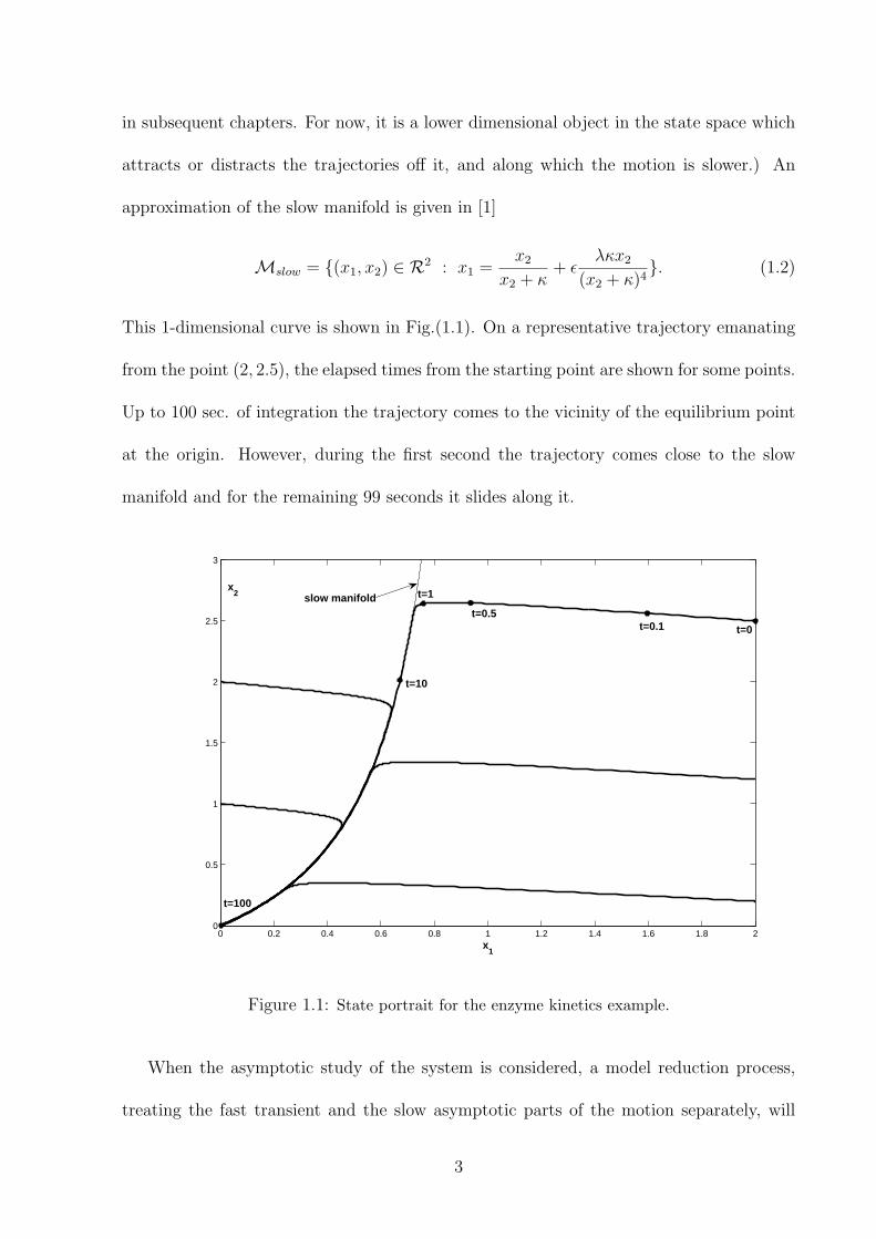
in subsequent chapters. For now, it is a lower dimensional object in the state space which
attracts or distracts the trajectories off it, and along which the motion is slower.) An
approximation of the slow manifold is given in [1]
Mslow = (x1, x2) ∈ R2 : x1 =x2
x2 + κ+ ε
λκx2
(x2 + κ)4. (1.2)
This 1-dimensional curve is shown in Fig.(1.1). On a representative trajectory emanating
from the point (2, 2.5), the elapsed times from the starting point are shown for some points.
Up to 100 sec. of integration the trajectory comes to the vicinity of the equilibrium point
at the origin. However, during the first second the trajectory comes close to the slow
manifold and for the remaining 99 seconds it slides along it.
0 0.2 0.4 0.6 0.8 1 1.2 1.4 1.6 1.8 20
0.5
1
1.5
2
2.5
3
x1
x2
t=0t=0.1t=0.5
t=1
t=10
t=100
slow manifold
Figure 1.1: State portrait for the enzyme kinetics example.
When the asymptotic study of the system is considered, a model reduction process,
treating the fast transient and the slow asymptotic parts of the motion separately, will
3

simplify the analysis. The “asymptotic” and “transient” parts of the trajectory can be
determined separately and pasted by using appropriate matching techniques. Potentially
the reduced models can be used to design controllers for slow and fast sub-systems that also
provide good stability and performance features for the original system when combined
appropriately. Since the core part of the system behavior takes place along the slow
manifold, any model reduction procedure would require to find the slow manifold.
1.2.2 Second Example: Optimal Control Problem
Consider the following optimal control problem. Minimize the cost
J(x, u) =∫ tf
0(x2 + u2)dt (1.3)
subject to the dynamical constraint
x = −x3 + u (1.4)
and the boundary constraintsx(0) = 1
x(tf ) = 1.5(1.5)
Applying the first-order necessary conditions for optimality leads to the following boundary
value problemx = −x3 − λ
2, x(0) = 1, x(tf ) = 1.5
λ = −2x + 3x2λ(1.6)
where λ = −∂H∂x
and H = x2 + u2 + λ(−x3 + u).
The solutions to this two-point boundary value problem computed by simple “shooting
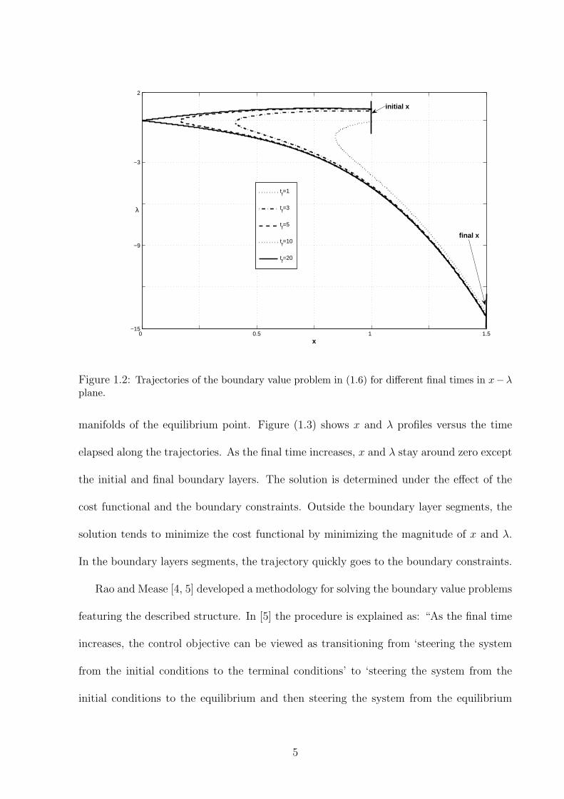
method”[3]. Figure (1.2) shows the optimal trajectories, the solutions of the boundary
value problem in (1.6), for some different final times.
For the dynamics in (1.6), the origin is a saddle type equilibrium point. As the final
time, tf , increases, the solution curves in x − λ plane approach the stable and unstable
4
0 0.5 1 1.5−15
−9
−3
2
x
λ
tf=1
tf=3
tf=5
tf=10
tf=20
initial x
final x
Figure 1.2: Trajectories of the boundary value problem in (1.6) for different final times in x−λplane.
manifolds of the equilibrium point. Figure (1.3) shows x and λ profiles versus the time
elapsed along the trajectories. As the final time increases, x and λ stay around zero except
the initial and final boundary layers. The solution is determined under the effect of the
cost functional and the boundary constraints. Outside the boundary layer segments, the
solution tends to minimize the cost functional by minimizing the magnitude of x and λ.
In the boundary layers segments, the trajectory quickly goes to the boundary constraints.
Rao and Mease [4, 5] developed a methodology for solving the boundary value problems
featuring the described structure. In [5] the procedure is explained as: “As the final time
increases, the control objective can be viewed as transitioning from ‘steering the system
from the initial conditions to the terminal conditions’ to ‘steering the system from the
initial conditions to the equilibrium and then steering the system from the equilibrium
5

0 2 4 6 8 10 12 14 16 18 200
0.5
1
1.5
2
t
x
0 2 4 6 8 10 12 14 16 18 20−15
−10
−5
0
5
t
λ
Figure 1.3: x vs. t and λ vs. t for the boundary value problem in (1.6).
to the terminal conditions’. Strictly speaking, this transition never takes place. How-
ever, assuming such a transition does occur, the problem can be decomposed into simpler
subproblems; the associated error decreases as the final time increases.”
Developing tools for diagnosing the existence of the aforementioned structures, slow,
stable, and unstable manifolds, in the state space or in a subset of the state space and
determining them, if they exist, requires the understanding of the geometric structures
around invariant manifolds in the state space. The next section provides introductory
information on how the geometric structure of the general nonlinear systems near compact
invariant manifolds can be obtained from the study of the structure of the associated
linearized problem. It starts with the trivial invariant set: isolated equilibrium point.
6

1.3 Geometric Structure of the Nonlinear Systems
Near Equilibrium Points and Compact Invariant
Manifolds
Consider the nonlinear dynamical system described by at least C1 vector field f(·) : Rn →
TRn
x = f(x) (1.7)
where x ∈ Rn and f(x) ∈ TxRn. In words, the vector field f(x) assigns a vector in the
tangent space of Rn at any point x ∈ Rn. The flow generated by this vector field, denoted
by φ(t, ·) : Rn →Rn, satisfies the differential equations in (1.7), i.e. φ(t, x) = f(φ(t, x)).
The nonlinear flow and vector field on Rn induce a linear flow and linear vector field on
the tangent bundle of Rn. When the nonlinear equations are linearized around a reference
trajectory φref (t, x), then the induced linear vector field is
δx =∂f
∂xδx = A(φref (t, x))δx = A(t)δx, where δx ∈ TxRn. (1.8)
The linear flow generated by the linear vector field in Eq. (1.8) is denoted by Φ(t, x)(·) :
TxRn → Tφref (t,x)Rn and is a map on the tangent bundle of Rn that maps a vector in TxRn
to a vector in Tφref (t,x)Rn, i.e. δx = Φ(t, x)δx0, where δx0 ∈ TxRn and δx ∈ Tφref (t,x)Rn.
When the nonlinear system is linearized around a non-stationary reference trajectory,
the induced linear vector field is linear time-varying (LTV). When the reference trajectory
is stationary, i.e., an equilibrium point of the nonlinear system, xeq, then the induced linear
vector field is linear time-invariant (LTI), i.e., A is a constant matrix
δx = Aδx. (1.9)
In general, Φ(t, x) ∈ Rn×n is the transition matrix and satisfies the LTV dynamics in
7

Eq. (1.8)
∂Φ(t, x)
∂t= A(t)Φ(t, x) (1.10)
with the initial condition Φ(0, x) = In. For the LTI dynamics the flow is determined by
δx = eAtδx0.
1.3.1 Geometric Structure of LTI Systems
For the LTI dynamics δx = Aδx the eigenvalues and eigenvectors of matrix A give the
information about the geometric structure of TxRn. Let the eigenvalues of A be distinct
for simplicity and assume that the eigenvalues are in increasing order, i.e. λ1 < ... < λn.
The eigenvectors corresponding to different eigenvalues constitute a set of basis vectors
which span the different subspaces of TxRn that form invariant subbundles of TRn. In
this context, the invariance condition can be written as Φ(t, x)ei = σ(t)ei, where ei is
the eigenvector corresponding to λi and σi(t) = eλit is a scaling factor. The invariance
can be seen from the following calculation of the transition matrix, which is the matrix
exponential in the LTI case
Φ(t, x) = eAt = I + At +1
2!A2t2 +
1
3!A3t3 + .... (1.11)
Eq. (1.11) shows that the eigenvectors of eAt are the eigenvectors of A and
Φ(t, x)ei = Iei+Aeit+1
2!A2eit
2+1
3!A3eit
3+.... = (1+λit+1
2!λi
2t2+1
3!λi
3t3+....)ei = eλitei
(1.12)
gives the desired relation.
The following subspaces of TxRn, called the stable eigenspace, unstable eigenspace,
and center eigenspace, respectively, are defined based on the sign of the eigenvalues, λ, of
8

A
Es = spanv : v is an eigenvector of A corresponding λ with Re(λ) < 0
Eu = spanv : v is an eigenvector of A corresponding λ with Re(λ) > 0
Ec = spanv : v is an eigenvector of A corresponding λ with Re(λ) = 0.
(1.13)
In case the eigenvectors are complex, then the generalized eigenvectors are used in the
definition of eigenspaces. The vectors in the stable eigenspace contract exponentially in
forward time, and the vectors in the unstable eigenspace expand exponentially in forward
time whereas they contract exponentially in backward time. The vectors in the center
eigenspace grow at most sub-exponentially both in forward and backward time.
These eigenspaces form a decomposition of TxRn
TxRn = Es ⊕ Ec ⊕ Eu. (1.14)
Another decomposition of TxRn can be obtained by grouping the eigenvalues of A in two
sets Spslow and Spfast such that |Reλi||Reλj| << 1 for all λi ∈ Spslow and λj ∈ Spfast assuming
the imaginary parts of λi and λj are not much different and using the following subspaces
Eslow = spanvi : λi ∈ Spslow
Efast = spanvi : λi ∈ Spfast., (1.15)
where Reλ is the real part of λ. Then, the decomposition can be written as
TxRn = Eslow ⊕ Efast. (1.16)
In this case, the rate of contraction or expansion of the vectors in Efast is much faster than
that of the vectors in Eslow.
9

1.3.2 Geometric Structure of Nonlinear Flow Near an Equilib-rium Point
Definition 1.3.1 (Hyperbolic Equilibrium Point) An equilibrium point, xeq, of the non-
linear flow determined by the vector field x = f(x) is hyperbolic provided that ∂f(xeq)∂x
has
no eigenvalues with zero real part.
Definition 1.3.2 (Stable and Unstable Manifolds of an Equilibrium Point of a Nonlinear
Flow) Let Nxeq denote a neighborhood of xeq. The local stable manifold is
W sloc(xeq) = x ∈ Nxeq : φ(t, x) ∈ Nxeq ∀t ≥ 0, φ(t, x) → xeq as t →∞. (1.17)
Similarly, the local unstable manifold is
W uloc(xeq) = x ∈ Nxeq : φ(t, x) ∈ Nxeq ∀t ≤ 0, φ(t, x) → xeq as t → −∞. (1.18)
The Hartman-Grobman Theorem and Stable and Unstable Manifold Theorems provide
the base for the analysis of nonlinear systems near an equilibrium point by analyzing the
induced linear system.
Theorem 1.3.3 (Hartman-Grobman Theorem For Equilibrium Point) If xeq is a hyper-
bolic equilibrium point of the nonlinear dynamics (1.7), then there exists a homeomorphism
defined on some neighborhood Nxeq of xeq, h : Nxeq → TxeqRn, mapping orbits of the non-
linear flow to orbits of the induced linear flow. The homeomorphism preserves the sense
of orbits and can also be chosen to preserve the parametrization by time.
Figure (1.4) illustrates the correspondence between the nonlinear and linearized flow ex-
plained by Hartman-Grobman Theorem.
10

Figure 1.4: Hartman-Grobman Theorem for equilibrium points.
See [6, 7] for a detailed study of Hartman-Grobman Theorem. When ∂f(xeq)∂x
has no eigen-
values with zero real part, the asymptotic behavior of solutions of x = f(x) near xeq is
determined by the linearization of x = f(x) around xeq. The Stable Manifold Theorem
gives the relation between the stable and unstable eigenspaces of the system in (1.8) and
the local stable and unstable manifolds of the system in (1.7) at the hyperbolic equilibrium
point of (1.7).
Theorem 1.3.4 (Stable Manifold Theorem for an Equilibrium Point) Suppose that xeq ∈
Rn is an isolated hyperbolic equilibrium point of the nonlinear system (1.7). Then there ex-
ist local stable and unstable manifolds, W sloc(xeq) and W u
loc(xeq), of the same dimensions as
the stable and unstable eigenspaces, respectively, of the linearized dynamics (1.8). W sloc(xeq)
and W uloc(xeq) are tangent to Es and Eu at xeq, respectively.
Figure (1.5) illustrates the local stable and unstable manifolds of an equilibrium point and
the associated eigenspaces for a 2-dimensional system.
11

Figure 1.5: Local stable and unstable manifolds of an equilibrium point and the associatedeigenspaces.
1.3.3 Geometric Structure of Nonlinear Flow Near a CompactInvariant Manifold
The geometric structure of the nonlinear flow φ(t, x) generated by the vector field x = f(x)
near a compact invariant submanifold M⊂ Rn is given by the Stable Manifold Theorem
for Invariant, Compact Manifolds which is the natural extension of that for equilibrium
points.
Definition 1.3.5 [8, 7](Normal Hyperbolic Manifold) The submanifold M is said to be
normally hyperbolic if the tangent bundle TRn restricted to M, denoted as TRn|(M),
decomposes at each point x ∈M as
TxRn = TxM⊕∆s(x)⊕∆u(x) (1.19)
where TxM denotes the tangent space to the submanifold M at x, ∆s(x) and ∆u(x) denote
the stable and unstable subspace at x which are invariant under the linear variational flow
Φ(t, x)(·) : TxRn|(M) → Tφ(t,x)Rn|(M) and there exist positive constants c and α such
12

that the properties
‖Φ(t, x)δx‖ ≤ c‖δx‖e−αt for all t > 0, x ∈M, δx ∈ ∆s(x)
‖Φ(t, x)δx‖ ≤ c‖δx‖eαt for all t > 0, x ∈M, δx ∈ ∆u(x)(1.20)
are satisfied
Theorem 1.3.6 [9, 8, 6](Stable Manifold Theorem for Normally Hyperbolic, Invariant,
Compact Manifolds) Suppose that the compact submanifold M ⊂ Rn is invariant under
the nonlinear flow φ(t, ·) generated by the vector field (1.7) and normally hyperbolic. Then
in a neighborhood NM of M, there exist locally invariant manifolds W sloc(M) and W s
loc(M)
with the properties
• TW sloc(M) = TM⊕∆s and TW u
loc(M) = TM⊕∆u,
• Points on the local stable and unstable invariant submanifolds asymptotically ap-
proach M when propagated by the nonlinear flow in forward and backward time,
respectively. W sloc(M) and W u
loc(M) can be defined as the union of the local stable
and unstable manifolds of the points on the invariant manifold MW s(M) =
⋃x∈M W s
loc(M, x)
W u(M) =⋃
x∈M W uloc(M, x)
(1.21)
where W sloc(M, x) (W u
loc(M, x)) is the fiber of W sloc(M) (W u
loc(M)) at point x ∈M.
• W sloc(M) and W u
loc(M) are invariantly fibered so that each fiber has the property
TxWsloc(M) = TxM ⊕ ∆s(x) and TxW
uloc(M) = TxM ⊕ ∆u(x) for all x ∈ M;
and if two points x1, x2 ∈ W sloc(M, x) (∈ W u
loc(M, x)) for some x ∈ M, then
φ(t, x1), φ(t, x2) ∈ W sloc(M, φ(t, x)) (∈ W u
loc(M, φ(t, x))), where φ(t, ·) is the flow
generated by f .
• Near M, f , is topologically conjugate to ∂f(x)∂x|(∆s ⊕∆u), i.e., there exists an home-
omorphism, defined on some neighborhood of M, mapping orbits in W sloc(M) ∪
13
W uloc(M) to orbits of the induced linear flow in ∆s ⊕ ∆u, preserving the sense of
orbits and the parametrization by time.
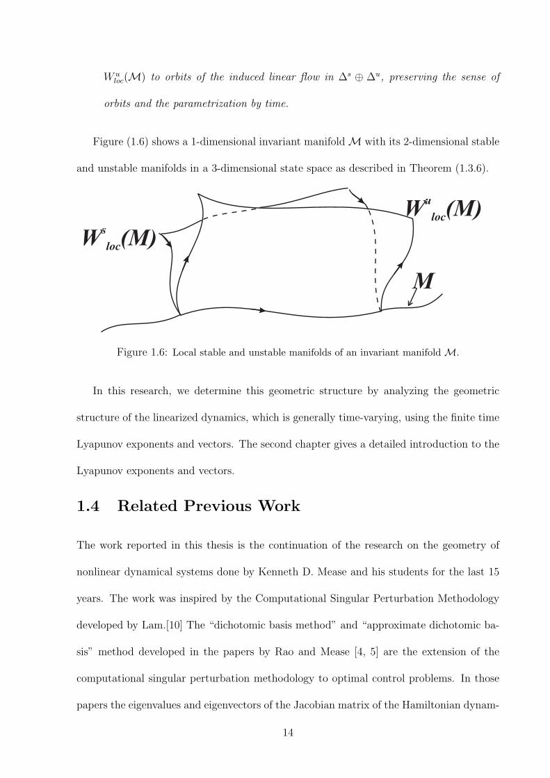
Figure (1.6) shows a 1-dimensional invariant manifold M with its 2-dimensional stable
and unstable manifolds in a 3-dimensional state space as described in Theorem (1.3.6).
Figure 1.6: Local stable and unstable manifolds of an invariant manifold M.
In this research, we determine this geometric structure by analyzing the geometric
structure of the linearized dynamics, which is generally time-varying, using the finite time
Lyapunov exponents and vectors. The second chapter gives a detailed introduction to the
Lyapunov exponents and vectors.
1.4 Related Previous Work
The work reported in this thesis is the continuation of the research on the geometry of
nonlinear dynamical systems done by Kenneth D. Mease and his students for the last 15
years. The work was inspired by the Computational Singular Perturbation Methodology
developed by Lam.[10] The “dichotomic basis method” and “approximate dichotomic ba-
sis” method developed in the papers by Rao and Mease [4, 5] are the extension of the
computational singular perturbation methodology to optimal control problems. In those
papers the eigenvalues and eigenvectors of the Jacobian matrix of the Hamiltonian dynam-
14

ics in the optimal control problems are used in order to describe the associated geometry
in state-costate space. More recently, the Lyapunov exponents and vectors have been used
as the accurate tools for analyzing the geometric structure of the linearization of the non-
linear dynamical systems around non-stationary reference trajectories.[8, 11, 12] In this
thesis Lyapunov exponents and vectors are used for determining the slow manifold in the
state space and for the “dichotomic basis method” and “approximate dichotomic basis
method” in determining the stable and unstable manifolds. The application to the slow
manifold determination is a new direction in this research aimed at model order reduction.
The application to the solution of the optimal control problems is an extension of the
previous work providing more accurate tools.
The singular perturbation theory is a well-developed methodology for model order
reduction based on the timescale separation in the dynamics. However, the tools of the
singular perturbation theory is only applicable if the dynamics are given in the special
form, so called “singularly perturbed form”. However, there is no general way to bring
a nonlinear system into singularly perturbed form. The understanding of the timescale
structure and the associated geometric structure through the study of Lyapunov exponents
and vectors may facilitate the applicability of the singular perturbation theory. A more
detailed discussion of the singular perturbation theory is given in Chapters (3) and (4).
Any model reduction mechanism based on the timescale separation in the system dy-
namics requires the knowledge of a possibly existing slow manifold. Besides the singular
perturbation methodology, there are other analytical and geometrical methods for deter-
mining the slow manifold. A survey on the existing methods is given in Chapter (3).
The indirect methods for solving optimal control problems suffer from the lack of a
full set of boundary conditions that can be used to integrate the system dynamics and
15

the volume-preserving nature of the dynamics. Coordinate transformations that decouple
the stable and unstable subsystems and suppress the unstable dynamics during the inte-
gration are used in literature. Our main contribution is to decouple these dynamics more
accurately by using the Lyapunov exponents and vectors. More detailed discussion on the
use of coordinate transformation and the use of singular perturbation theory for solving
optimal control problems is given in Chapter (4).
16

Chapter 2
Lyapunov Exponents and TangentSpace Structure
In this chapter the tools for diagnosing the timescale structure and determining its asso-
ciated tangent space structure on a compact invariant subset Y of Rn are introduced and
modified in order to use them to obtain similar information for a compact non-invariant
subset X of Rn.
2.1 Terminology, Assumptions, and Evolution Equa-
tions
The scenario is that a dynamical system is given in a particular coordinate representation
and the objective is to diagnose whether or not multiple-timescale behavior exists, and if
it does, to determine the associated geometric structure, particularly the slow, stable and
unstable manifolds. The state coordinate vector is x ∈ Rn and the dynamics are
x = f(x), (2.1)
where the vector field f is assumed continuously differentiable. We refer to Eq. (2.1) as
the x-representation of the dynamical system. It will be important to distinguish between
inherent system properties that would be observed in any coordinate representation and
properties that are specific to a particular coordinate representation. We express the
17

solution of Eq. (2.1) for the initial condition x(0) = x0 as x(t) = φ(t, x0), where φ is the
transition map or flow satisfying ∂φ/∂t = f(φ(t, x0)) and φ(0, x0) = x0. In the state space
view, φ maps x0 along the trajectory (i.e., solution) through that point, t units of time to
the point x(t). If t > 0, this is forward propagation; if t < 0, this is backward propagation.
Controlled dynamical systems are of interest, but the explicit dependence of f on a
control function is not addressed. Timescale analysis of x = f(x) is relevant for a controlled
system in each of the following cases: (i) the control function is determined by a feedback
law and f(x) represents the closed-loop dynamics, (ii) f(x) is the open-loop dynamics
and the plan is to use low-gain control which would not alter the time-scale structure, or
(iii) x = f(x) is the Hamiltonian system for an optimally controlled system, x being the
combined state and co-state vector (see Chapter (4)).
The linearized dynamics associated with Eq. (2.1) are
v = J(x)v, (2.2)
where J = ∂f/∂x. We will analyze the linearized dynamics to characterize the timescales
in the nonlinear dynamics. In general, we need to consider Eqs. (2.1) and (2.2) as a
coupled system, because J(x) depends on x. An initial point (x, v) is mapped in time t to
the point (x(t), v(t)) = (φ(t, x), Φ(t, x)v), where Φ is the transition matrix for the linearized
dynamics, defined such that Φ(0, x) = I, the n × n identity matrix. Geometrically, each
point x in the state space is a base point of a tangent space, in which v takes values. The
coordinates for v correspond to a tangent space frame, whose axes are parallel to those
of the x-frame, but with origin at x. Our analysis will concern a domain Y ⊂ Rn of
the state space. The tangent space at a point x ∈ Y is denoted by TxY . The tangent
bundle TY is defined as the union of the tangent spaces over Y , and (x, v) is a point
in the tangent bundle, with v the tangent vector and x the base point. We need the
18

interpretation (x, v) ∈ TY because the analysis of the linearized dynamics will define a
subspace decomposition in the tangent space and the orientation of the subspaces will vary
with the base point x.
If we have k linearly independent vector fields w1(x), . . . , wk(x) defined on Y that
vary continuously with x, we can define at each x a k-dimensional subspace Λ(x) =
spanw1(x), . . . , wk(x). If k = n, then Λ(x) = TxY and for each x the vector fields
provide a basis for TxY . If k < n, then Λ(x) is a linear subspace of TxY and Λ is called a
distribution on Y . A distribution is invariant if for any x ∈ Y and v ∈ Λ(x), the property
Φ(t, x)v ∈ Λ(φ(t, x)) holds for any t such that φ(t, x) ∈ Y . Distributions Γ1, . . . , Γm allow
a splitting of the tangent space, if TxY = Γ1(x) ⊕ . . . ⊕ Γm(x), where ⊕ denotes the
direct sum of linear subspaces; in words, each vector in TxY has a unique representation
as a linear combination of vectors, one from each of the subspaces Γ1(x), . . . , Γm(x) and
Γi(x)∩Γj(x) = 0 for all i 6= j, where 0 is the set whose only element is the zero vector.
If each distribution in the splitting is invariant, then the splitting is called an invariant
splitting.
If a collection of r ≤ n linear subspaces of TxY can be ordered such that Λ1(x) ⊂
Λ2(x) ⊂ ... ⊂ Λr(x) = TxY , then this collection of nested proper subspaces defines a
filtration of TxY . Note that the subspaces of the filtration satisfy for i = 1, ..., r − 1 the
condition dimΛi(x) < dimΛi+1(x).
A smooth submanifold[13] M ⊂ Rn of dimension k < n, for which M∩ Y is non-
empty, is relatively invariant with respect to Y for the vector field x = f(x), if for any
x ∈M∩Y , φ(t, x) ∈M if φ(t, x) ∈ Y . This means a trajectory emanating from any point
in M∩Y remains on M in forward and backward time as long as the trajectory is in Y .
An equivalent requirement for relative invariance is that f(x) ∈ TxM for all x ∈ M∩ Y ,
19

which means that the trajectory through x is tangent to M and will thus stay on M.
2.2 Lyapunov Exponents and Vectors
First introduced by Lyapunov [14] in order to study the stability of non-stationary solutions
of ordinary differential equations, Lyapunov exponents are measures of the average expo-
nential rate of growth/decay of functions. For a real valued function g(t) the Lyapunov
exponent is given by
µ[g] = lim supt→∞
1
tln |g(t)|. (2.3)
Lyapunov exponents provide a generalization of the linear stability analysis using perturba-
tions from stationary solutions to that using perturbations from non-stationary solutions.
Lyapunov exponents have found extensive applications in mathematics, dynamical systems
theory and physics especially in the study of chaos since they are measures of the sensitiv-
ity of solutions of dynamical systems to small perturbations from the nominal solutions.
A positive exponent indicates chaotic behavior. In this context Lyapunov exponents have
been extensively used in the study of fluid flow mechanisms[15, 16] and forecasting[17].
They have also been used in trajectory tracking law design[18].
Our goal is to obtain timescale information and the associated geometric structure of
the nonlinear system in Eq.(2.1) by studying the linearized dynamics in Eq.(2.2). The
dynamics in Eq.(2.2) are linear time-varying because of the x(t) dependence of J matrix
and x is the solution of the nonlinear dynamics. The Lyapunov exponents for the LTV
dynamics in Eq.(2.2) are given as [19]
µ+(x, v) = lim supT→∞
1
Tln(‖Φ(T, x)v‖
‖v‖ ) (2.4)
for each x ∈ Y and nonzero v ∈ TxY , where v is a solution of Eq.(2.2). Lyapunov also
identified the subclass of LTV systems called regular LTV systems, for which the Lyapunov
20
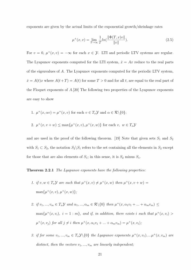
exponents are given by the actual limits of the exponential growth/shrinkage rates
µ+(x, v) = limT→∞
1
Tln(‖Φ(T, x)v‖
‖v‖ ). (2.5)
For v = 0, µ+(x, v) = −∞ for each x ∈ Y . LTI and periodic LTV systems are regular.
The Lyapunov exponents computed for the LTI system, x = Ax reduce to the real parts
of the eigenvalues of A. The Lyapunov exponents computed for the periodic LTV system,
x = A(t)x where A(t+T ) = A(t) for some T > 0 and for all t, are equal to the real part of
the Floquet exponents of A.[20] The following two properties of the Lyapunov exponents
are easy to show
1. µ+(x, αv) = µ+(x, v) for each v ∈ TxY and α ∈ R\0;
2. µ+(x, v + w) ≤ maxµ+(x, v), µ+(x, w) for each v, w ∈ TxY
and are used in the proof of the following theorem. [19] Note that given sets S1 and S2
with S1 ⊂ S2, the notation S2\S1 refers to the set containing all the elements in S2 except
for those that are also elements of S1; in this sense, it is S2 minus S1.
Theorem 2.2.1 The Lyapunov exponents have the following properties:
1. if v, w ∈ TxY are such that µ+(x, v) 6= µ+(x,w) then µ+(x, v + w) =
maxµ+(x, v), µ+(x,w);
2. if v1, ..., vm ∈ TxY and α1, ..., αm ∈ R\0 then µ+(x, α1v1 + ... + αmvm) ≤
maxµ+(x, vi), i = 1 : m, and if, in addition, there exists i such that µ+(x, vi) >
µ+(x, vj) for all j 6= i then µ+(x, α1v1 + ... + αmvm) = µ+(x, vi);
3. if for some v1, ..., vm ∈ TxY\0 the Lyapunov exponents µ+(x, v1), ...µ+(x, vm) are
distinct, then the vectors v1, ..., vm are linearly independent;
21
4. the function (Lyapunov exponent) µ+ attains no more than n distinct finite values.
By statement 4 of Thm.(2.2.1) the forward Lyapunov exponents can take on at most n
distinct values on TxY\0. For simplicity we assume that µ+ takes on exactly n distinct
values on TxY\0, i.e. there is no repeated Lyapunov exponent. We further assume that
these distinct values of Lyapunov exponents are ordered as
µ+1 < ... < µ+
n . (2.6)
It is important to note that for a given trajectory of a regular dynamical system the
Lyapunov exponents are independent of the starting point, because they are asymptotic
measures of the average exponential rate of growth/decay of functions.
The linear subspaces L+i (x), defined as
L+i (x) = v ∈ TxY : µ+(x, v) ≤ µ+
i , i = 1, 2, ..., n (2.7)
with L+0 = 0, form the following filtration of TxY
0 = L+0 ⊂ L+
1 (x) ⊂ L+2 (x) ⊂ ... ⊂ L+
n (x) = TxY . (2.8)
Theorem 2.2.2 [19] Let L+i (x), i = 1, ..., n be the filtration defined in (2.7) and (2.8).
Then the following properties hold:
1. µ+(x, v) ≤ µ+i for every v ∈ L+
i (x);
2. µ+(x, v) = µ+i for every v ∈ L+
i (x)\L+i−1(x).
Another representation of the L+i (x) subspaces can be constructed as follows: Let the
one dimensional subspace L+1 (x) be spanned by the unit vector l+1 (x), a vector in Rn
called the Lyapunov vector corresponding to µ+1 at x. Then, define another unit vector
l+2 (x), called the Lyapunov vector corresponding to µ+2 at x, orthogonal to l+1 (x) such that
22
L+2 (x) = spanl+1 (x), l+2 (x). Continuing this procedure creates a new representation of
the subspaces in (2.7):
L+1 (x) = spanl+1 (x),
L+2 (x) = spanl+1 (x), l+2 (x),
...L+
i (x) = spanl+1 (x), l+2 (x), ..., l+i (x),...
L+n (x) = spanl+1 (x), l+2 (x), ..., l+n (x).
(2.9)
Example 2.2.3 To gain more insight into the filtration in (2.8), consider a two-dimensional
nonlinear system with Y = xeq, xeq an equilibrium point. Assume the linearized dynam-
ics at xeq are characterized by distinct eigenvalues λf and λs, with λf << λs < 0, and
corresponding eigenvectors ef and es. The Lyapunov exponents are equal to the eigenval-
ues, i.e., µ+1 = λf and µ+
2 = λs, and the Lyapunov vector l+1 (xeq) corresponding to µ+1 aligns
with the eigenvector ef corresponding to λf . The second Lyapunov vector l+2 is in the di-
rection of e⊥f , the vector perpendicular to ef . The subspace L+1 (xeq) is Ef (xeq) = spanef,
the eigenspace for λf , whereas L+2 (xeq) = TxeqX . It would be desirable instead to obtain
the decomposition TxeqX = Ef (xeq)⊕Es(xeq) where Es(xeq) = spanes. However, as the
averaging time T goes to ∞, all the vectors not in L+1 (xeq) have the Lyapunov exponent
µ+2 = λs; thus the Lyapunov exponents for forward time propagation do not distinguish Es.
The way to obtain Es is by repeating the same analysis for backward time propagation; in
this case, the situation is reversed and Es can be distinguished, whereas Ef cannot.[21]
Eigenspaces are invariant under the linear dynamics in that an initial tangent vector in
an eigenspace will remain in that eigenspace under forward or backward propagation, and
TxeqX = Ef (xeq)⊕ Es(xeq) is an example of an invariant splitting.
In order to define a new filtration to be able to capture Es, let’s first define the backward
23
Lyapunov exponents
µ−(x, v) = limT→∞
1
Tln(‖Φ(−T, x)v‖
‖v‖ ). (2.10)
For v = 0, µ−(x, v) = −∞ for each x ∈ Y . The backward Lyapunov exponents satisfy all
the properties stated for the forward Lyapunov exponents in Thm. (2.2.1). Assume that
they are distinct and the distinct values are ordered as
µ−n < ... < µ−1 . (2.11)
Then similar to the filtration defined in terms of the forward Lyapunov exponents, the
subspaces
L−i (x) = v ∈ TxY : µ−(x, v) ≤ µ−i , i = 1, 2, ..., n (2.12)
comprise another filtration of TxY with L+n+1 = 0
0 = L−n+1 ⊂ L−n (x) ⊂ L−n−1(x) ⊂ ... ⊂ L−1 (x) = TxY . (2.13)
Theorem 2.2.4 Let L−i (x), i = 1, ..., n be the filtration defined in (2.12) and (2.13).
Then the following properties hold:
1. µ−(x, v) ≤ µ−i for every v ∈ L−i (x);
2. µ−(x, v) = µ−i for every v ∈ L−i (x)\L−i−1(x).
Similar to the forward subspaces, another representation of the backward subspaces
can be generated by setting L−n (x) = spanl−n (x), where l−n (x) is the backward Lyapunov
vector corresponding to µ−n at x, and repeating the procedure in (2.9) in the reverse
directionL−n (x) = spanl−n (x),
L−n−1(x) = spanl−n (x), l−n−1(x),...
L−i (x) = spanl−n (x), l−n−1(x), ..., l−i (x),...
L−1 (x) = spanl−n (x), l−n−1(x), ..., l−1 (x).
(2.14)
24

Now back to the Example (2.2.3), Es(xeq) can be identified as L−2 (xeq), and es and
l−2 (xeq) are in the same direction. Fig.(2.1) shows the eigenvectors and Lyapunov vectors
for the Example (2.2.3).
Figure 2.1: Eigenvectors and Lyapunov vectors of the systems in Example (2.2.3).
Having defined the forward and backward Lyapunov exponents and filtration in terms
of the Lyapunov exponents we are ready to state the following characterization of the
regularity.
Definition 2.2.5 [11, 19] The system is regular at x, if and only if
i) the forward and backward Lyapunov exponents exist as the limits,
ii) µ+i = −µ−i , i = 1, ...n;
iii) the forward and backward filtrations have the same dimension;
iv) there exists a decomposition TxY = E1(x) ⊕ ... ⊕ En(x) into invariant sub-bundles
such that L+i (x) = E1(x)⊕ ...⊕ Ei(x) and L−i (x) = Ei(x)⊕ ...⊕ En(x), i = 1, ..., n;
25

v) for any v ∈ Ei(x)\0, limT→∞ ln‖Φ(±T,x)v‖‖v‖ = ±µ+
i .
Note that in dynamical system literature and particularly in [19, 20] equivalent definitions
are given in terms of the Lyapunov exponents of the adjoint linear system, ˙v = −JT (x)v.
This equivalence will be shown in the following section after the finite time Lyapunov
exponents and vectors are introduced.
Computation of the Lyapunov Exponents: By the definition of the subspaces
L+i (x) any unit vector in the subspace L+
i (x)\L+i−1(x) has the Lyapunov exponent µ+
i , i.e.
for v ∈ L+i (x)\L+
i−1(x)
µ+(v, x) = limT→∞
1
Tln‖Φ(T, x)v‖ = µ+
i . (2.15)
The claim is that most of the tangent vectors in the tangent space at x are in the subspace
v ∈ L+i (x)\L+
i−1(x). Let’s try to visualize this in a 2-dimensional setting. In 2-dimensions
all the vectors except l+1 (x) are in the subspace v ∈ L+2 (x)\L+
1 (x). If by chance it is not
in L+2 (x)\L+
1 (x), then a vector in L+2 (x)\L+
1 (x) can be found with at most 2 trials by
keeping one component and changing the other one. Similarly, in the n dimensional case
any arbitrarily chosen vector is most probably in L+n (x)\L+
n−1(x). If it is not, a vector in
L+n (x)\L+
n−1(x) can be found with at most n trials. Consequently, the largest Lyapunov
exponent can be computed by Eq.(2.15) by taking an arbitrary tangent vector v ∈ TxY
assuming that it is not in L+n (x)\L+
n−1(x). The calculation of the next Lyapunov expo-
nent is not straightforward since any arbitrary vector chosen will not be in the subspace
L+n−1(x)\L+
n−2(x). However, most of the subspaces spanned by any two linearly indepen-
dent unit vectors will be in the subspace L+n (x)\L+
n−2(x). Let two unit tangent vectors
vn and vn−1 at x be arbitrarily chosen. Then, the sum of the greatest two Lyapunov
26

exponents is given by
µ+n + µ+
n−1 = limT→∞
1
Tln(An,n−1) (2.16)
where An,n−1 is the area of the parallelogram determined by Φ(T, x)vn and Φ(T, x)vn−1.
Once the largest Lyapunov exponent is known the second largest can be calculated from
Eq.(2.16). Repeating this computation the ith Lyapunov exponent can computed from
µ+n + µ+
n−1 + ... + µ+i = lim
T→∞1
Tln(An,i) (2.17)
where An,i is the volume of the parallelogram determined by
Φ(T, x)vn, Φ(T, x)vn−1, ..., Φ(T, x)vi, (2.18)
and vn, vn−1, ..., vi are n− i + 1 arbitrarily chosen tangent vectors at x.
The backward Lyapunov exponents can be computed by following the same proce-
dure in backward time. However, once again note that the computation of the Lyapunov
exponents requires infinite averaging time, which is not feasible in practical applications.
Theorem 2.2.6 [22] The distributions
Λ+i (x) = spanl+1 (x), ..., l+i (x)
Λ−i (x) = spanl−n (x), ..., l−i (x),(2.19)
where l+1 (x), ..., l+i (x) are the column vectors of L+i (x), and l−n (x), ..., l−i (x) are the col-
umn vectors of L−i (x), are invariant distributions, i.e., for any v ∈ Λ+i (x) , Φ(t, x)v ∈
Λ+i (φ(t, x)), and for any v ∈ Λ−i (x), Φ(t, x)v ∈ Λ−i (φ(t, x)) for all t.
The proof of the theorem is based on the property that the Lyapunov exponents are
constants on trajectories of Eq.(2.1) and can be found in [22]. We do not repeat the proof;
but give a sketch of the proof in order to clarify what the invariance of the subspaces
means. The proof equivalently shows the following: For any x ∈ Y and t ∈ R
〈Φ(t, x)l+i (x), l+j (φ(t, x))〉 =
0, if i < jnonzero, if i ≥ j
(2.20)
27

where 〈·, ·〉 denotes the inner product and 1 ≤ i, j ≤ n. In words, it says when a vector
v ∈ spanl+1 (x), l+2 (x), ..., l+i (x) is propagated by the transition matrix Φ(t, x), then the
propagated vector will not have a component in the direction of l+j (φ(t, x)) for any j > i.
Thus, the distributions spanned by the basis vectors of the subspaces L+i (x), i = 1, ..., n
are invariant distributions on Rn. Similarly for the backward Lyapunov vectors, for any
x ∈ Y and t ∈ R
〈Φ(t, x)l−i (x), l−j (φ(t, x))〉 =
0, if i > jnonzero, if i ≤ j
(2.21)
where 1 ≤ i, j ≤ n. Therefore, the distributions spanned by the basis vectors of the
subspaces L−i (x), i = 1, ..., n are invariant distributions on Rn.
The Lyapunov exponents and vectors provide tools for correctly analyzing the timescale
structure and the associated tangent space geometry in LTV systems [19, 21, 11]. Example
(2.2.7), which is from [12], compares the timescale information obtained by using the
Lyapunov exponents and vectors and that obtained by the eigenvalues and eigenvectors of
Jacobian and transition matrices.
Example 2.2.7 The purpose of this example is to distinguish clearly between the timescale
information provided by the Lyapunov exponents and vectors and the information from
the eigenvalues and eigenvectors of the transition matrix and the local Jacobian matrix.
Consider the linear, time-invariant system
w = Λw =
[λf 00 λs
]w (2.22)
where w = (w1, w2)T and the eigenvalues of Λ are real with λf << λs < 0. We introduce
the coordinate transformation
x = R(t)w =
[cos θ(t) − sin θ(t)sin θ(t) cos θ(t)
]w (2.23)
28
where θ = ωt and ω is a constant. In terms of x, the system is
x = A(t)x = (RRT + RΛRT )x = R(RT R + Λ)RT x (2.24)
The transition matrix for the w-system is eΛt, whereas the transition matrix for the x-
system is
Φ = R(t)eΛt (2.25)
In the w-representation the behavior is composed of fast and slow exponentially contracting
modes with fixed directions given by the eigenvectors of Λ. In the x-representation there
are also fast and slow exponentially contracting modes, but the fast and slow directions
are rotating. From the SVD of Φ, we will show that the Lyapunov exponents and vectors
identify the slow and fast exponential modes. In contrast, we will show that eigenvalues
and eigenvectors for A(t) and Φ do not. Our interest is not directly in linear time-varying
systems, but this example serves as an idealization of the linearized dynamics of a nonlin-
ear system whose slow and fast directions rotate as one traverses the state space along a
trajectory, as would be the case along a trajectory on a slow manifold with curvature.
Φ has the SVD: Φ = L−Σ+(L+)T = R(t) exp(Λt)I, where I is the 2×2 identity matrix.
The singular values are the positive square roots of the eigenvalues of ΦT Φ = exp(2Λt),
and clearly the rotational motion does not influence them. The Lyapunov exponents are
µ+1 = λf and µ+
2 = λs and are independent of t for this example, so any averaging time
will give the same Lyapunov exponents. For the time interval (t1, t2), the SVD is Φ =
R(t2) exp(Λ(t2 − t1))RT (t1); thus we have L+(t) = L−(t) = R(t). Note that here t is not
an averaging time argument. If there were some underlying nonlinear dynamics, whose
linearization gives the LTV dynamics in Eq.(2.23), then t would be an argument that
indicates the base point in the state space at which the Lyapunov vectors are computed. The
SVD of Φ identifies the exponential rates of the two modes in Σ+ and the rotating directions
29

of these modes in L+ and L−. Specifically we have the fast subspace Ef (t) = L+1 (t) =
spanl+1 (t) and the slow subspace Es(t) = L−2 (t) = spanl−2 (t), where the fast direction
is l+1 (t) = [cos θ(t) sin θ(t)]T and the slow direction is l−2 (t) = [− sin θ(t) cos θ(t)]T . In
this example the rotational motion is periodic and Floquet theory is applicable; but, the SVD
would also characterize different and irregular rotations of the fast and slow directions.
The eigenvalues of A(t) = (RRT + RΛRT ) are[23] the same as the eigenvalues of the
matrix
(RT R + Λ) =
[λf −ωω λs
](2.26)
because the two matrices are related by a similarity transformation. The two eigenvalues
are
λ(A(t)) =1
2
(λf + λs ±
((λf − λs)
2 − 4ω2)1/2
)(2.27)
and are denoted by λ+ and λ− based on which sign is taken. The corresponding eigenvectors
of A(t) are
v+(A(t)) = R(t)
[−ω
λ+(A(t))− λf
]v−(A(t)) = R(t)
[λ−(A(t))− λs
ω
](2.28)
The eigenvalues of Φ(t) are
λ(Φ(t)) =1
2
(cos(ωt)(eλf t + eλst)±
(cos2(ωt)(eλf t + eλst)2 − 4e(λf+λs)t
)1/2)
(2.29)
The eigenvalues of A(t) and Φ(t) depend on the rotation rate ω. For A(t), the eigenvalues
are independent of t for this example. As ω increases from zero the eigenvalues approach
each other, becoming equal when ω = (λs − λf )/2, and then split as a complex conjugate
pair. For a given value of ω, the eigenvalues of Φ depend on cos ωt. At times for which
cos ωt = 0, the eigenvalues are pure imaginary. Only at times for which cos ωt = 1 are the
eigenvalues λ− = eλf t and λ+ = eλst. Hence, in general, neither the eigenvalues of A nor
Φ are reliable indicators of the fast and slow exponential modes.
30

The main purpose of this work is to compute the slow, stable and unstable manifolds as-
sociated with the timescale structure, if such structure exists. When the Lyapunov vectors
(more specifically the subspaces spanned by the appropriate Lyapunov vectors) are used,
then these manifolds can be calculated with no error, as we will show on a 2-dimensional
example in the next chapter. However, no practical method to determine Lyapunov ex-
ponents and vectors emerges from the previous analysis because existing theory considers
asymptotic behavior using infinite time limits on an invariant subset of the phase space.
Furthermore, it assumes the regularity of the system. On the other hand, most of the
problems motivating this research, e.g. guidance problems often formulated as optimal
control problems, are posed for a finite time interval and on a compact subset that is not
necessarily invariant. Even if longer averaging times are available, the sampling will be
outside of the region of interest because of the region is non-invariant. The timescale in-
formation outside of the region may be different than that inside of the region and change
the computed timescale information. Moreover, on non-invariant sets it is not possible to
assume that the system under consideration is regular. The techniques we will develop do
not require a strict compatibility between the forward and backward Lyapunov exponents
as in the second property in the Definition (2.2.5).
When the subset is not invariant, the timescales and the associated geometric structure
characteristics of the flow on the subset must be computable on finite-time trajectory
segments. In the next section, a method for extracting the timescale information and its
associated tangent space structure on a compact non-invariant subset is presented.
31

2.3 Finite Time Lyapunov Exponents and Vectors
Existing dynamical systems theory[19] for manifold structure in the state space considers
an invariant set and is based on asymptotic properties. Rates of tangent vector contraction
and expansion are characterized by Lyapunov exponents defined as limits when t → ∞
or t → −∞. In sharp contrast, our interest is in timescale structure on a compact region
X that is not invariant and thus only accommodates finite averaging times. The behavior
outside of X may be different than that inside X , so we do not want the Lyapunov
exponents to be influenced by behavior outside of X . Hence we use finite-time Lyapunov
exponents to characterize the rates of contraction and expansion and finite-time Lyapunov
vectors to characterize the tangent space structure. Fortunately, a timescale gap that
induces tangent space structure also ensures that structure is computable.
We consider in particular the system behavior on an n-dimensional compact subset
X ⊂ Y . For example, X could be generated by choosing a closed sphere Ω ∈ Y of initial
conditions for x, centered on the initial point in the state space for a nominal trajectory,
and then integrating Eq. (2.1) for time Tc to yield X = x ∈ Y :x = φ(t, x0) for some
t ∈ [0, Tc] and x0 ∈ Ω. For each x ∈ X , there is a maximal time interval T (x) = [t¯(x), t(x)]
which includes zero, such that φ(t, x) ∈ X for all t ∈ T (x). The minimum time to reach
transversely the boundary of X from x is t(x) for forward time propagation and t¯(x) for
backward time propagation. If x is on the boundary of X , then one of these times can be
zero. If the trajectory never leaves X in forward time, then t(x) is taken to be infinite, and
similarly for backward time. If t(x) = ∞ for all x ∈ X , then X is a positively invariant set
for the dynamics under consideration; if t(x) = −∞ for all x ∈ X , then X is a negatively
invariant set; and if T (x) = (−∞,∞) for all x ∈ X then X is an invariant set. We include
the possibility of X being an invariant set, even though our interest is in the non-invariant
32

case, because we want to connect our developments to existing dynamical systems theory.
A sphere of initial conditions for v ∈ TxX , propagated along a trajectory of the non-
linear system for time T according to the linearized dynamics, evolves into an ellipsoid. A
vector v0 ∈ Tx0X , propagated for T units of time along the trajectory φ(t, x0), evolves to
the vector vT = Φ(T, x0)v0 in the tangent space Tφ(T,x0)X . To simplify the notation, the
subscript “0” will not be used further; rather x and v will be used to denote the initial
state and tangent vectors.
The ratio of the Euclidean lengths of an initial non-zero vector and its corresponding
final vector, σ = ‖vT‖/‖v‖, is a multiplier that characterizes the net expansion (growth),
if σ > 1, or contraction, if σ < 1, of the vector over the time interval (0, T ). The
propagation time T is always taken to be positive whether forward or backward. The
forward and backward finite-time Lyapunov exponents are given by
µ+(T, x, v) = 1T
ln σ+(T, x, v) = 1T
ln ‖Φ(T,x)v‖‖v‖
µ−(T, x, v) = 1T
ln σ−(T, x, v) = 1T
ln ‖Φ(−T,x)v‖‖v‖
(2.30)
for propagation time T > 0. For v = 0, define µ+(T, x, 0) = µ−(T, x, 0) = −∞. A
Lyapunov exponent allows the corresponding multiplier to be interpreted as an average
exponential rate, i.e., σ = exp(µ · T ).
Discrete forward and backward Lyapunov spectra, for each (T, x), can be defined in
terms of the extremal values of the forward and backward exponents, respectively. For
forward propagation, these extremal values are the exponents for the unit vectors in TxX
that map to the principal axes of an ellipsoid in Tφ(T,x)X , and there are at most n distinct
extremal values for each (T, x).
One way to obtain the extremal exponents is to compute the singular value decompo-
33

sition (SVD) of Φ(T, x) = N+(T, φ(T, x))Σ+(T, x)L+(T, x)T , where
Σ+(T, x) =
σ+1 (T, x)
. . .
σ+n (T, x)
(2.31)
contains the singular values and the ordering is such that σ+1 (T, x) ≤ σ+
2 (T, x) ≤ . . . ≤
σ+n (T, x), and to compute the extremal Lyapunov exponents as µ+
i (T, x) = (1/T ) ln σ+i (T, x),
i = 1, . . . , n. The column vectors of L+(T, x) are denoted l+i (T, x), i = 1, . . . , n are
the finite time Lyapunov vectors and the column vectors of N+(T, φ(T, x)) are denoted
n+i (T, φ(T, x)), i = 1, . . . , n are the principal axes of the ellipsoid in Tφ(T,x)X . Rearranging
the SVD of Φ(T, x), we can write Φ(T, x)l+i (T, x) = exp(µ+i (T, x)T )n+
i (T, φ(T, x)) which
indicates that l+i (T, x) ∈ TxX whereas n+i (T, φ(T, x)) ∈ Tφ(T,x)X .
Similarly for backward propagation, the extremal values are the exponents for the unit
vectors in TxX that map to principal axes of an ellipsoid in Tφ(−T,x)X . The backward
extremal exponents can be obtained from the singular value decomposition Φ(−T, x) =
N−(T, φ(−T, x))Σ−(T, x)L−(T, x)T , assuming the ordering on the diagonal of Σ−(T, x) is
such that σ−1 (T, x) ≥ . . . ≥ σ−n (T, x), by µ−i (T, x) = (1/T ) ln σ−i (T, x), i = 1, . . . , n. The
column vectors of L−(T, x) denoted by l−i (T, x), i = 1, . . . , n are backward finite time
Lyapunov vectors. For the column vectors of L−(T, x) and N−(T, φ(−T, x)), we have
l−i (T, x) ∈ TxX whereas n−i (T, φ(−T, x)) ∈ Tφ(−T,x)X .
In summary, a sphere of tangent vectors in TxX is propagated T units of time forward
to an ellipsoid in Tφ(T,x)X and backward to another ellipsoid in Tφ(−T,x)X . In TxX , the
l+i (T, x) vectors propagate to the principal axes of the forward ellipse, whereas the l−i (T, x)
vectors propagate to the principal axes of the backward ellipse. See Fig.(2.2) for the case
of n = 1. The finite time Lyapunov vectors, will be used to define subspaces in TxX with
different exponential rates.
34
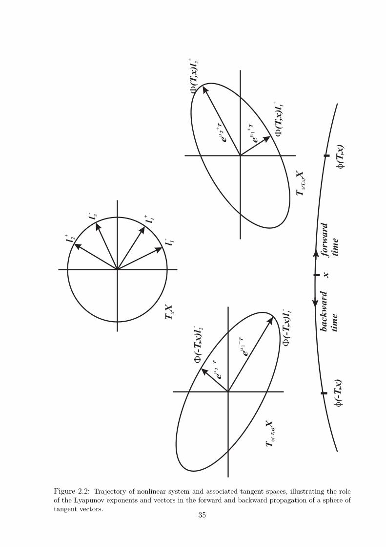
Figure 2.2: Trajectory of nonlinear system and associated tangent spaces, illustrating the roleof the Lyapunov exponents and vectors in the forward and backward propagation of a sphere oftangent vectors.
35

A note on the uniqueness of the singular value decomposition: The assump-
tion that the Lyapunov exponents are ordered as µ+1 (T, x) ≤ ... ≤ µ+
n (T, x) is not only for
simplicity, but it is also required for the uniqueness of singular value decomposition of the
transition matrix. An assumption for the ordering of the exponents, i.e., entries of Σ in
Φ = NΣLT , assures the uniqueness of N , Σ, and L.
Relations between the forward and backward exponents and vectors over
the same trajectory segment: It is known that for the LTV systems the transition
matrix has the property [Φ(t, t0)]−1 = Φ(t0, t) where t0 is the time at which the propagation
begins and t is the time at which the propagation ends. In our notation, this relation can be
written as Φ(T, x) = Φ(−T, φ(T, x))−1. Using this relation and the SVD of each transition
matrix as
Φ(T, x) = N+(T, φ(T, x))Σ+(T, x)L+(T, x)T
Φ(−T, φ(T, x)) = N−(T, x)Σ−(T, φ(T, x))L−(T, φ(T, x))T ,(2.32)
the following relations between forward and backward exponents and vectors over the same
trajectory segment can be written
n+i (T, φ(T, x)) = l−i (T, φ(T, x));
µ+i (T, x) = −µ−i (T, φ(T, x));
l+i (T, x) = n−i (T, x).
(2.33)
Figure (2.3) illustrates these relations.
Relations between the backward exponents and the exponents of the adjoint
system over the same trajectory segment: The adjoint system of a linear system,
δx = Aδx, is δ ˙x = −AT δx. It can be shown that Φ(t, t0;−AT ) = [Φ(t, t0; A)]−T [20]. Let
Φ(t, t0;−AT ) be denoted by Φ∗(t, t0). Thus, Φ∗(T, x) = Φ(T, x)−T = Φ(−T, φ(T, x))T .
By equating the SVDs of Φ∗(T, x) and Φ(−T, φ(T, x))T , the following relations can be
36

Figure 2.3: Correspondence between the backward and forward N and L matrices computedfrom the SVD of the transition matrix.
obtainedΣ∗(T, x) = Σ−(T, φ(T, x))
L∗(T, x) = N−(T, x)
N∗(T, φ(T, x)) = L−(T, φ(T, x)).
(2.34)
Using these relations and the fact that the infinite time Lyapunov exponents are constant
along the trajectories, we can verify that in the definition of regularity we stated earlier the
backward exponents and the exponents of the adjoint systems can be used equivalently.
Optimization problem interpretation of the Lyapunov exponents and vec-
tors: It can be shown that the columns of L+(T, x), the vectors that map to the principal
axes of the ellipsoid at the point φ(T, x), are the right singular vectors of Φ(T, x) by solving
the following constrained optimization problem.
extremize vT Φ(T, x)T Φ(T, x)v over v
subject to vT v = 1(2.35)
By using a Lagrange multiplier λ, the Lagrangian can be written as
L(v, λ) = vT Φ(T, x)T Φ(T, x)v+ λ(1− vT v).
Differentiating L with respect to v, Φ(T, x)T Φ(T, x)v∗ = λv∗, where v∗ is the opti-
mizing solution, can be written. Thus, the optimizing solution v∗ is an eigenvector of
Φ(T, x)T Φ(T, x). Consequently, it is a right singular vector of Φ(T, x) [24]. The solution
37

to the following extremization problem gives the columns of L−(T, x)
extremize vT Φ(−T, x)T Φ(−T, x)v over v
subject to vT v = 1.(2.36)
Similar extremization problems can be used in order to define the infinite time Lya-
punov exponents and vectors for regular systems. For example, the solution to the problem
extremize limT→∞ 1T
ln ‖Φ(T, x)v‖ over v
subject to ‖v‖ = 1(2.37)
is the vectors l+i (x), i = 1, ..., n. The regularity assures that the following limits exists
and the vectors l+i (x), i = 1, ..., n and the Lyapunov exponents µ+i can be computed as
the eigenvectors and the eigenvalues of
limT→∞
[Φ(T, x)T Φ(T, x)]1/2T . (2.38)
Despite the fact that Lyapunov exponents are constant along the trajectories and
Lyapunov vectors are only functions of the base point x ∈ X , the finite time Lyapunov
exponents and vectors depend on both the base point and the averaging time.
To simplify the presentation, we assume that the forward and backward extremal ex-
ponents are distinct for all T and x. The column vectors of L+(T, x) and the column
vectors of L−(T, x) finite time Lyapunov vectors each provide orthonormal bases for TxX .
The following subspaces, for i = 1, . . . , n, can be defined by the Lyapunov vectors
L+i (T, x) = spanl+1 (T, x), . . . , l+i (T, x)
L−i (T, x) = spanl−i (T, x), . . . , l−n (T, x).(2.39)
Proposition 2.3.1 The subspaces L+i (T, x) and L−i (T, x) have the properties:
i) v ∈ L+i (T, x)\0 ⇒ µ+(T, x, v) ≤ µ+
i (T, x)
ii) v ∈ L−i (T, x)\0 ⇒ µ−(T, x, v) ≤ µ−i (T, x).
38

Proof: Let v be a unit vector in spanl+1 (T, x), . . . , l+i (T, x). v can be decomposed as
v = a1l+1 (T, x)+ ...+ail
+i (T, x) where a2
1 + ...+a2i = 1. The finite time Lyapunov exponent
of v can be written as µ+(T, x, v) = 1T
ln(a2
1e2µ+
1 (T,x)T + ... + a2i e
2µ+i (T,x)T
)1/2by using the
orthogonality of the Lyapunov vectors, the property of the Lyapunov vectors that they
are unit length by definition, and the equality Φ(T, x)l+i (T, x) = eµ+i (T,x)T n+
i (T, φ(T, x)).
Since a21e
2µ+1 (T,x)T + ... + a2
i e2µ+
i (T,x)T is a convex combination of e2µ+1 (T,x)T , ..., e2µ+
i (T,x)T ,
µ+(T, x, v) is less than µ+i (T, x). The proof of the second property in the proposition is
similar to the proof of the first property just T is replaced by −T . 2
Similar to the filtrations formed by Lyapunov vectors, the subspaces defined in terms
of the finite time Lyapunov vectors form filtrations as
0 = L+0 ⊂ L+
1 (T, x) ⊂ L+2 (T, x) ⊂ ... ⊂ L+
n (T, x) = TxX
TxX = L−n (T, x) ⊃ L−n−1(T, x) ⊃ ... ⊃ L−n (T, x) ⊃ L−n+1 = 0(2.40)
The feasibility of determining timescale structure depends on whether the structure of
primary interest converges, as the averaging time increases, within the available range of
averaging times. Next section is devoted to the convergence properties of the finite time
Lyapunov exponents and vectors. The convergence of the finite time Lyapunov vectors is
based on the existence of a sufficiently large spectral gap.
2.4 Convergence Properties of the Finite Time Lya-
punov Exponents and Vectors
The finite time Lyapunov exponents do not converge to the Lyapunov exponents in gen-
eral. The discussion in the section (2.2) is given for the Lyapunov regular systems. For
the Lyapunov regular systems the forward and backward finite time Lyapunov exponents
converge with the increasing averaging time and are of opposite signs. The relations be-
39
tween the finite time Lyapunov exponents and their infinite time limits for the forward
and backward cases are
limT→∞ µ+i (T, x) = µ+
i , i = 1, ..., n,
limT→∞ µ−i (T, x) = µ−i = −µ+i , i = 1, ..., n.
(2.41)
A less restrictive requirement is the convergence of the backward and forward finite
time Lyapunov exponents as the averaging time tends to ∞, but not necessarily to the
values of opposite sign. If the forward and backward finite time Lyapunov exponents
converge, then the system is called forward and backward regular, respectively. In this
case the relations between the finite time Lyapunov exponents and Lyapunov exponents
arelimT→∞ µ+
i (T, x) = µ+i , i = 1, ..., n,
limT→∞ µ−i (T, x) = µ−i , i = 1, ..., n.(2.42)
2.4.1 Differential equations of the finite time Lyapunov expo-nents and vectors with respect to the averaging time
Goldhirsch et al.[25] developed the evolution equations for the finite time Lyapunov expo-
nents µ+i (T, x) and the finite time Lyapunov vectors l+i (T, x).
Lemma 2.4.1 [11] Over intervals of the averaging time T during which the finite time
Lyapunov exponents are distinct, the finite time Lyapunov exponents and vectors at x ∈ X
evolve with the averaging time T according to the differential equations
∂
∂Te2µ+
i (T,x)T = e2µ+i (T,x)T l+i (T, x)T QT [J(T )T + J(T )]Ql+i (T, x), (2.43)
∂∂T
l+i (T, x) =∑i−1
k=1l+k
(T,x)T QT [J(T )T +J(T )]Ql+i (T,x)
e(µ+
i(T,x)−µ+
k(T,x))T−e
(µ+k
(T,x)−µ+i
(T,x))Tl+k (T, x) + ciil
+i (T, x)
+∑n
k=i+1l+k
(T,x)T QT [J(T )T +J(T )]Ql+i (T,x)
e(µ+
i(T,x)−µ+
k(T,x))T−e
(µ+k
(T,x)−µ+i
(T,x))Tl+k (T, x).
(2.44)
where J(T ) = J(x(T )) and Q = Q(T, x) = N+(T, φ(T, x))L+(T, x)T are function of
averaging time T and the state x. The coefficient cii is determined such that l+i (T, x)
evolves continuously with unit length.
40

Note that replacing Q by Q(T, x) = N+(T, φ(T, x))L+(T, x)T gives
Ql+i (T, x) = n+i (T, φ(T, x)). (2.45)
because of the mutual orthogonality and unit length properties of the Lyapunov vectors.
A similar result for backward finite time Lyapunov exponents and vectors can be de-
rived. It is given in the next lemma.
Lemma 2.4.2 Over intervals of the averaging time T during which the finite time Lya-
punov exponents are distinct, the finite time Lyapunov exponents and vectors at x ∈ X
evolve with the averaging time T according to the differential equations
∂
∂Te2µ−i (T,x)T = −e2µ−i (T,x)T l+−(T, x)T QT [J(−T )T + J(−T )]Ql−i (T, x), (2.46)
∂∂T
l−i (T, x) = −∑i−1k=1
l−k
(T,x)T QT [J(−T )T +J(−T )]Ql−i (T,x)
e(µ−
i(T,x)−µ−
k(T,x))T−e
(µ−k
(T,x)−µ−i
(T,x))Tl−k (T, x)− ciil
−i (T, x)
−∑nk=i+1
l−k
(T,x)T QT [J(−T )T +J(−T )]Ql−i (T,x)
e(µ−
i(T,x)−µ−
k(T,x))T−e
(µ−k
(T,x)−µ−i
(T,x))Tl+k (T, x)
(2.47)
where J(−T ) = J(x(−T )) and Q = Q(T, x) = N−(T, φ(T, x))L−(T, x)T are function of
averaging time T and the state x. The coefficient cii is determined such that l−i (T, x)
evolves continuously with unit length.
2.4.2 Convergence properties
Definition 2.4.3 For an n-dimensional dynamical system on a compact set X with finite-
time Lyapunov exponents ordered as µ+1 (T, x) < µ+
2 (T, x) < . . . < µ+n (T, x), neighboring
exponents µ+j (T, x) and µ+
j+1(T, x) for a particular value j are temporally uniformly distinct
at x, if there exists a T independent spectral gap ∆µ+(x) > 0 and an averaging time
Tmin(x) such that µ+j+1(T, x) − µ+
j (T, x) > ∆µ+(x) for all T ∈ T (x)\[−Tmin(x), Tmin(x)].
Tmin(x) is introduced to eliminate any initial transient period that is not representative of
the subsequent behavior and should be small relative to the available averaging time. If
41

µ+j and µ+
j+1 are temporally uniformly distinct for all x ∈ X and there exists a positive
constant ∆µ such that ∆µ < ∆µ(x) for all x ∈ X , then we say there is a uniform spectral
gap on X . A uniform spectral gap for the neighboring backward time exponents µ−k−1 and
µ−k is similarly defined.
Theorem 2.4.4 [11]If the neighboring Lyapunov exponents µ+j (T, x) and µ+
j+1(T, x) are
temporally uniformly distinct at the point x, then as T increases, the subspace L+j (T, x)
converges toward a fixed subspace L+j (x) at least at the rate 1/(e∆µ+·T − e−∆µ+·T ) where
∆µ+(x) is the spectral gap. Similarly, if µ−k−1(T, x) and µ−k (T, x) are temporally uniformly
distinct at x, then as T increases, the L−k (T, x) converges toward a fixed subspace L−k (x)
at least at the rate 1/(e∆µ−·T − e−∆µ−·T ) where ∆µ−(x) is a bound on µ−k−1 − µ−k over T .
The proof of Theorem (2.4.4) given in [11, 25]. It is based on Lemma (2.4.1) and Lemma
(2.4.2). The term l+k (T, x)T Q[F (T )T + F (T )]Ql+i (T, x) in Eq.(2.4.1) can be bounded us-
ing the continuity of F (T )T + F (T ) on the compact set X and the fact that the Lya-
punov vectors have unit length. Thus, the coefficients of l+j (T, x), ..., l+n (T, x) for the rates
of change of l+1 (T, x), ..., l+j (T, x) are bounded by a function which decays at the rate
1/(e∆µ+·T − e−∆µ+·T ). To see this, let l+k (T, x)T Q[F (T )T + F (T )]Ql+i (T, x) be bounded by
B > 0 for all T , i.e., ‖l+k (T, x)T Q[F (T )T + F (T )]Ql+i (T, x)‖ ≤ B. Then, for k > i
l+k (T, x)T QT [J(T )T + J(T )]Ql+i (T, x)
e(µ+i (T,x)−µ+
k(T,x))T − e(µ+
k(T,x)−µ+
i (T,x))T≤ B
(e∆µ+·T − e−∆µ+·T ), (2.48)
which decays at the rate 1/(e∆µ+·T − e−∆µ+·T ).
Summarizing, the subspaces L+i (T, x) converge to fixed subspaces at the rate 1/(e∆µ+·T−
e−∆µ+·T ), meaning that the components of the vectors in L+i (T, x) in the directions that
are not in the converged fixed subspace decay at that rate. The finite time Lyapunov
vectors may or may not converge. If they converge, their convergence is slower than the
42

rate 1/(e∆µ+·T − e−∆µ+·T ); in fact l+j (T, x), j = 1, ..., i converge at a rate related to the
difference of µ+j (T, x) from µ+
j−1(T, x) and µ+j+1(T, x). If µ+
j (T, x), j = 1, ..., n are uni-
formly distinct with a spectral gap ∆µ+j , then the individual finite time Lyapunov vectors
converge at the rate 1/(e∆µ+j ·T − e−∆µ+
j ·T ).
The question whether the converged fixed subspaces are the subspaces spanned by the
(infinite time) Lyapunov vectors has been raised by Goldhirsch et al. [25] and answered
that the finite time subspaces converge to the infinite time subspaces by showing that
the relation Φ(t, x)l+i (∞, x) ∝ eµ+i ·t holds for large t. Therefore, when the subspaces
L+i (T, x), i = 1, ..., n spanned by the finite time Lyapunov vectors converge the following
limits can be written
limT→∞
L+i (T, x) = L+
i (x), i = 1, ..., n, (2.49)
and when the individual finite time Lyapunov vectors converge
limT→∞
l+i (T, x) = l+i (x), i = 1, ..., n. (2.50)
For the systems whose finite time Lyapunov exponents converge, the following relation
is conjectured and tested numerically in [25]
µ±i (T, x) = µ±i +bi + ξi(T )
T, (2.51)
where bi is constant and ξi(T ) is the “noise” term whose time average is zero. Thus, al-
though the convergence rate of the finite time Lyapunov vectors (or the subspaces spanned
by the finite time Lyapunov vectors) is exponential, the convergence of the finite time Lya-
punov exponents, when they converge, is at a slower rate 1/T . The convergence of the
finite time Lyapunov exponents and vectors is illustrated in the next example.
43

Example 2.4.5 Consider the second order nonlinear differential equations
x1 = (1 + 2a(x1 + x2))λs(x1 − a(x1 + x2)2) + 2a(x1 + x2)λf (x2 + a(x1 + x2)
2).
x2 = −2a(x1 + x2)λs(x1 − a(x1 + x2)2) + (1− 2a(x1 + x2))λf (x2 + a(x1 + x2)
2).(2.52)
where a = 0.01, and λs and λf are constants. This nonlinear system has been used in
[11, 26] and it has been shown that the finite time Lyapunov exponents converge for λs =
−1 and λf = −10. Figure (2.4) shows the Lyapunov exponents and the angles between
l+i (T, x), i = 1, 2, and l−i (T, x), i = 1, 2 and the horizontal axis for λs = −1 and λf =
−10, − 3. For both cases, the finite time Lyapunov exponents converge. For λf = −10,
they converge to −10 and −1 and the gap is 9, whereas for λf = −3, they converge to −3
and −1 and the gap is 2. Since the gap is smaller in the case of λf = −3 than that in the
case of λf = −10, a slower convergence of the finite time Lyapunov vectors in the case
of λf = −3 is expected. The last two plots in Fig. (2.4) show indeed that the finite time
Lyapunov vectors in the case of λf = −3 converge at a slower rate.
2.5 Practical Invariance of Finite Time Distributions
Definition 2.5.1 (Practically Invariant Distribution) Let ξ1 (x) , ξ2 (x) , ..., ξn (x) be a ba-
sis for TxX , and ξ1 (x) , ξ2 (x) , ..., ξm (x), m ≤ n span a distribution Λ(x) on TX . In
general, Φ(t, x)Λ(x) is spanned by ξi (φ(t, x)) , i = 1, ..., n. Let v be any nonzero vector in
Λ(x). If these exist ε > 0 and t1, t2 > 0 such that
maxv∈Λ(x)
‖Φ (t, x) v − ΠΛ (Φ (t, x) v)‖‖Φ (t, x) v‖ ≤ ε (2.53)
for all t ∈ [−t1, t2], and ΠΛ is the projection on the subspace Λ(φ(t, x)), then Λ(x) is a
practically invariant distribution of the order of ε on [−t1, t2] under the linear flow.
ε is the level of accuracy with which the subspace Λ(T, φ(t, x)) is required to approximate
the subspace Φ(t, x)Λ(x).
44
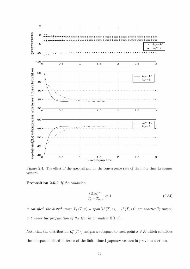
0 0.5 1 1.5 2 2.5 3−15
−10
−5
0
5
Lyap
unov
exp
onen
ts
λf=−10
λf=−3
0 0.5 1 1.5 2 2.5 330
35
40
45
50
angle
bet
ween
l+ 1(T,x)
and
hor
izont
al ax
is
λf=−10
λf=−3
0 0.5 1 1.5 2 2.5 340
45
50
55
60
T, averaging time
angle
bet
ween
l+ 2(T,x)
and
hor
izont
al ax
is
λf=−10
λf=−3
Figure 2.4: The effect of the spectral gap on the convergence rate of the finite time Lyapunovvectors.
Proposition 2.5.2 If the condition
(∆µi)−1
Tc − Tmin
¿ 1 (2.54)
is satisfied, the distributions ÃL+i (T, x) = spanl+1 (T, x), ..., l+i (T, x) are practically invari-
ant under the propagation of the transition matrix Φ(t, x).
Note that the distribution L+i (T, ·) assigns a subspace to each point x ∈ X which coincides
the subspace defined in terms of the finite time Lyapunov vectors in previous sections.
45

Proof: The proof will be given only for n = 2 and only for the distribution L+1 (T, x).
The distribution L+2 (T, x) = TxX = R2 is trivially invariant. A generalization for higher
dimensions will be explained. In the 2-dimensional case the practically invariant distri-
bution is the span of l+1 (T, x). Since it is a linear subspace at each point x, the practical
invariance of l+1 (T, x) suffices the practical invariance of its span. Pre-multiplication of
Φ(−T, φ(T, x))l−1 (T, φ(T, x)) = eµ−1 (T,φ(T,x))T l+1 (T, x) by Φ(t, x) yields to
Φ(−(T − t), φ(T, x))l−1 (T, φ(T, x)) = eµ−1 (T,φ(T,x))T Φ(t, x)l+1 (T, x). (2.55)
By using the singular value decomposition of Φ(−(T − t), φ(T, x)) one can write the fol-
lowing equation.
[l+1 ((T − t), φ(t, x))T
l+2 ((T − t), φ(t, x))T
]T
diag(eµ−i ((T−t),φ(T,x))(T−t))
[l−1 ((T − t), φ(T, x))T
l−2 ((T − t), φ(t, x))T
]l−1 (T, φ(T, x))
= eµ−1 (T,φ(T,x))T Φ(t, x)l+1 (T, x).(2.56)
Now let θ be the angle between l−1 (T − t, φ(T, x)) and l−1 (T, φ(T, x))
θ = 6 (l−1 (T − t, φ(T, x)), l−1 (T, φ(T, x))). (2.57)
Since l−1 ((T − t), φ(T, x))T l−1 (T, φ(T, x)) = cosθ and l−2 ((T − t), φ(T, x))T l−1 (T, φ(T, x)) =
sinθ one can write the following equation by doing the multiplications in the last equation.
eµ−1 (T,φ(T,x))T Φ(t, x)l+1 (T, x) = cosθeµ−1 ((T−t),φ(T,x))(T−t)l+1 ((T − t), φ(t, x))
+ sinθeµ−2 ((T−t),φ(T,x))(T−t)l+2 ((T − t), φ(t, x)).
(2.58)
Now let α be the angle 6 (Φ(t, x)l+1 (T, x), l+1 ((T − t), φ(t, x))). From Eq. (2.58)
tan α =sinθ
cosθ
eµ−2 ((T−t),φ(T,x))(T−t)
eµ−1 ((T−t),φ(T,x))(T−t)≤ sinθ
cosθe−∆µ(T−t). (2.59)
By Theorem (2.4.4), the Lyapunov vector l−1 (T, φ(T, x)) converges exponentially fast.
Thus, there exists T > t∗ > 0 such that sinθcosθ
≤ 1 for all t ∈ [0, t∗]. Consequently, tanα ≤
46

e−∆µ(T−t) for all t ∈ [0, t∗]. The exponential decay in the angle between l−1 (T, φ(T, x))
and its infinite time limit actually shows that t∗ is not much less than T . Due to the
trigonometric relation sinα ≤ tanα in the first quadrant and the fact that l+1 (T, x) was
arbitrary in the span of itself, the condition in Eq. (2.53) is satisfied with ε = e−∆µ(T−t).2
The propagation time can either be positive or negative, corresponding to forward
propagation and backward propagation, respectively. Although e−∆µ(T−t) provides a tight
bound in the case of the distribution spanned by the forward Lyapunov vectors for all
negative times, it grows exponentially in forward time. Thus, practical invariance of
forward distributions under the propagation of the transition matrix makes sense in the
interval t ∈ [t(x), t2], where t2 depends on the accuracy level, ε, required and the available
averaging time. The averaging time, T, the forward propagation duration, t2, should be
such that e−∆µ(T−t) ≤ ε, for all t ∈ [t(x), t2], i.e., e−∆µ(T−t2) ≤ ε.
In higher dimensions the proof follows the same with an arbitrary unit vector v in
L+i (T, x). In this case bounds for tanαj are exponentially decaying with increasing T and
exponentially growing with increasing propagation time t, where
αj = 6(Πij(Φ(t, x)v), l+j (T − t, φ(t, x))
), j = 1, ..., i, i = i + 1, ..., n, (2.60)
and Πij(·) is the projection on the subspace spanned by l+j (T − t, φ(t, x)) and l+i (T −
t, φ(t, x)). These angles decay exponentially with increasing T and Φ(t, x)v converges to a
vector in the subspace Li(T − t, φ(t, x)) exponentially with T , if the condition in Eq.(2.54)
is satisfied.
Figure (2.5) visualizes the proof for the 3 dimensional case where the practically invari-
ant distribution is 2 dimensional, i.e., the spectral gap is between the largest and second
largest exponent.In this case the decay of α1 and α2 is enough to show that Φ(t, x)v is
close to the subspace spanned by l+1 (T − t, φ(t, x)) and l+2 (T − t, φ(t, x)). A similar result
47

l2+(T−t,φ(t,x))
l3+(T−t,φ(t,x))
l1+(T−t,φ(t,x)) Φ(t,x)v
Π23
(Φ(t,x)v)
Π13
(Φ(t,x)v)
α1
α2
Figure 2.5: Illustration of the proof of the practical invariance for a 3 dimensional system witha spectral gap between µ+
2 and µ+3 .
can be stated for the distributions spanned by the backward time Lyapunov vectors.
Proposition 2.5.3 If the condition in Eq.(2.54) is satisfied, the distributions L−i (T, x) , i =
1, ..., n are practically invariant under the propagation of the transition matrix Φ(t, x).
Although e−∆µ(T−t) provides a tight bound in the case of the distribution spanned by the
backward time. Thus, practical invariance of backward distributions under the propagation
of the transition matrix makes sense in the interval t ∈ [−t1, t(x)], where t1 depends on
the accuracy level, ε, required and the available averaging time.
The practical invariance of L+1 (T, x) = spanl+1 (T, x) is illustrated in a 2-dimensional
example (2.5.4).
Example 2.5.4 Consider again the system in Example (2.4.5). By the equation
Φ(T, x)l+1 (T, x) = eµ+1 (T,x)T n+
1 (T, φ(T, x)) = eµ+1 (T,x)T l−1 (T, φ(T, x)), (2.61)
48

if the vector l+1 (T, x) is propagated by Φ(t, x) for T units of time Φ(T, x)l+1 (T, x) and
l−1 (T, φ(T, x)) are in the same direction. For the propagation times between 0 and T ,
Φ(T, x)l+1 (T, x) cannot in general be written equal to the finite time Lyapunov vectors at
φ(t, x) with an averaging time T . However, by Proposition (2.5.2) the propagated Lyapunov
vector Φ(T, x)l+1 (T, x) should be close to the Lyapunov vector at that point l+1 (T, φ(T, x))
for the propagation times that constitute a large fraction of the available averaging time.
This is what we call the practical invariance and the span of l+1 (T, x) is the practically
invariant subspace. The first plot in Fig.(2.6) shows that the direction of Φ(T, x)l+1 (T, x0)
is very close to the direction of l+1 (T, φ(t, x0)) for the initial 2.5 units of propagation time
of 3 units of averaging time. Then, it quickly diverges from that direction and aligns with
l−1 (T, φ(T, x0)) at the final time. The second plot in Fig.(2.6) shows that the angle between
Φ(T, x)l+1 (T, x0) and l+1 (T, φ(t, x0)) is relatively small for the initial 2.5 units of propagation
time compared to that in the rest of the 3 units of time .
2.6 Computation of Lyapunov Exponents and Vec-
tors
The most widely used methods for the computation of the Lyapunov exponents and vectors
are based on two matrix decompositions of the transition matrix Φ(T, x) namely
• Singular value decomposition (SVD),
• QR decomposition.
Each method is subclassified as
• Continuous method,
• Discrete method.
49

0 0.5 1 1.5 2 2.5 3−40
−20
0
20
40
60
80
degr
ee
t, time along the trajectory starting at x0
0 0.5 1 1.5 2 2.5 30
2
4
6
8
10
12
t, time along the trajectory starting at x0
degr
ee
absolute value of the anglebetween Φ(t,x
0)l+
1(3,x
0) and
l+1(3,φ(t,x))
the angle between l−
1(3,φ(3,x
0))
and the horizontal axis
the angle between Φ(t,x
0)l+
1(3,x
0)
and the horizontal axis
the angle between l+
1(3,φ(t,x
0))
and the horizontal axis
Figure 2.6: Illustration of the practical invariance in a 2 dimensional nonlinear example.
The SVD and its use in the computation of the Lyapunov exponents and vectors are
studied in section (2.3). In summary, the SVD of the transition matrix
Φ(T, x) = N+(T, Φ(T, x))Σ+(T, x)L+(T, x) (2.62)
gives the information of which directions in a unit sphere in the tangent space at point x
evolve to the principal axes of an ellipsoid in the tangent space at point φ(T, x) and the
length of the principal axes of the ellipsoid. The columns of L+(T, x) are the directions
in the tangent space at x that have extremal average expansion/shrinkage rates over the
50

period 0 − T . Note that these directions are not necessarily the directions of extremal
expansion/shrinkage for the averaging times less than T . However, they quickly converge
to some fixed directions as T increases under certain circumstances given in section (2.4).
The columns of N+(T, φ(T, x)) are the directions of the principal axes of the ellipsoid in
the tangent space at φ(T, x).
Another matrix decomposition used for the computation of Lyapunov exponents is the
QR decomposition of the transition matrix. It provides the information how the volumes
Vk of k-dimensional parallelepipeds in the tangent space Tφ(t,x)X ⊂ Rn, where k ≤ n,
change. Consider n arbitrarily chosen orthogonal unit vectors u1, ..., un in TxX . The
choice of ui = (0, ..., 0, 1, 0, ..., 0)T , where the i-th element is one, is almost standard. Let
pi ∈ Tφ(T,x)X be pi = Φ(T, x)ui. Then, the QR decomposition of the transition matrix
Φ(T, x) is given by [27]
Φ(T, x) = Q(T, x)R(T, x)
= [q1 ... qn]
R11 ∗ . . . ∗0 R22
. . ....
.... . . . . . ∗
0 . . . 0 Rnn
,(2.63)
where R is an upper triangular matrix and Q is an orthogonal matrix such that Q =
[q1 ..., qn]. q1, ..., qn are obtained by applying a Gram-Schmidt orthogonalization to
p1, ..., pn such that p1 and q1 are in the same direction. Figure(2.7) illustrates this ge-
ometry in 2-dimensional case. Then, the volume of the parallelepiped at point φ(T, x)
is
Vk =k∏
i=1
Ri×i, (2.64)
since the volume at x is one.
Note that the SVD and the QR decomposition do not give the same information for
finite times. Thus, the finite time Lyapunov exponents are not accessible from the Q and R
51

Figure 2.7: Illustration of the QR decomposition method for a 2 dimensional system.
matrices. However, some further manipulation of Q and R yields the finite time exponents
and vectors. To see this, start with the SVD and QRD of the transition matrix
Φ = QR = NΣLT . (2.65)
Using the orthogonality of L and N matrices, Σ = NT QRL. By the orthogonality of Q
and N , ΣT Σ gives
ΣT Σ = LT (RT R)L. (2.66)
Consequently, the eigenvalues of RT R are σ2i and the columns of L are the eigenvectors of
RT R.
When the finite time Lyapunov exponents converge, then the Lyapunov exponents are
given by
µ+i = lim
T→∞1
Tln(Rn−i+1×n−i+1). (2.67)
Roughly speaking, the difference between the discrete and continuous methods is the
order of integration and matrix decomposition. In discrete methods, Eqs. (2.1) and (2.2)
52

are integrated with the given initial conditions and the matrix decomposition is performed
at the averaging times of interest. In continuous methods, the differential equations for
the appropriate matrices among Q, R, N , Σ, and L or the entries of these matrices are
integrated in order to obtain the timescale information at the averaging times of interest.
Detailed information on the continuous methods can be found in [26, 28, 27, 29, 30, 31].
In the numerical computation of the transition matrix the columns of the transition
matrix become linearly dependent as T increases. Therefore, it is necessary to re-initialize
the integration of the Eq. (2.2) periodically and use the composition property of the
transition matrix
Φ(T + ∆T, x) = Φ(∆T, φ(T, x))Φ(T, x). (2.68)
In order to compute Φ(T, x), the time interval 0 − T is discretized as 0 = T0 < T1 <
T2 < ... < Ti < ... < TN = T and the Eqs. (2.1) and (2.2) are integrated with the
conditions x(Ti) = xi and Φ(0, φ(Ti, x(0))) = Φ(0, xi) = In×n. Then, the transition matrix
is calculated by
Φ(T, x) = Φ(TN − TN−1, φ(TN−1, x(0))Φ(TN−1 − TN−2, φ(TN−2, x(0)) ... Φ(T1 − T0, x(0)).
(2.69)
The re-initialization of the integration of the linearized equations reduces the accumulation
of the integration error.
For the computation of the Lyapunov exponents, when the finite time Lyapunov expo-
nents converge, let ∆T be such that Tj−Tj−1 = ∆T, j = 1, 2, ... where Tj are the times at
which the integration of the linearized equations is re-initialized and let the QRD of the
transition matrix from Tj−1 to Tj be
Φ(Tj − Tj−1, φ(Tj−1, x(0)) = QjRj. (2.70)
53
Then, the Lyapunov exponents can be calculated as [26, 28]
µ+i = lim
j→∞1
Tj
ln |(Rj)ii...(R1)ii|. (2.71)
More detail on the implementation of the QRD based discrete method can be found in
[26, 28, 27]. Although the exponents computed using the QRD based method are not the
same as the exponents using the SVD based method for finite times, they become the same
asymptotically [27, 32].
Comments on the methods for computing the Lyapunov exponents and
vectors
• The integration of the differential equations in the continuous methods should be
done by using special integrators (e.g. unitary integrators) that preserve the orthog-
onality [28].
• The differential equations in case of the continuous SVD method become singular
when there exist repeated Lyapunov exponents. This can be seen from the differential
equations (2.43) and (2.44). Although we assumed that the Lyapunov exponents are
distinct in our work, this may still cause numerical problems when the Lyapunov
exponents are close to each other but not equal.
• Continuous methods are computationally more costly [27].
• Discrete methods have difficulties in computing the large negative Lyapunov expo-
nents as the averaging time increases.
54

Chapter 3
Slow Manifold Determination inTwo-Timescale Nonlinear DynamicalSystems
3.1 Introduction to the problem and literature
Disparate timescales in the behavior of a dynamical system can induce a manifold structure
in the state space – an organizational structure for the trajectories of the system. In a
two-timescale system which has fast and slow behaviors, there may be an invariant slow
manifold which attracts trajectories emanating from initial states off this manifold. A slow
manifold may also be repelling in that trajectories from initial states off the manifold are
attracted to it in backward time, i.e., they depart in forward time. In fact the existence
of a slow manifold only requires that each trajectory in the neighborhood of the manifold
either depart from or approach the manifold at a rate that is significantly faster than the
rates at which trajectories on the manifold evolve [33]. When a slow manifold is attracting
for some initial conditions in forward time and attracting for other initial conditions in
backward time, it is called normally hyperbolic [21].
The existence of a slow manifold presents an opportunity for reduced-order analysis and
design. For example, in the case of an attracting slow manifold, the long-term behavior
of the system is governed by the dynamics on the slow manifold, because the trajectory
55
through any point off the slow manifold quickly approaches the slow manifold and then
stays on it. More precisely, the trajectory asymptotically approaches a trajectory on the
slow manifold, but in a practical sense the two trajectories are indistinguishable after a
fast initial transient phase.
Let us say that the slow manifold exists for a particular choice of state variables (i.e.,
system coordinates). In a different set of coordinates, obtained by a transformation that
does not alter the timescales [11], the same qualitative state space structure would exist
with certain properties the same and others altered – for example, there would be a slow
manifold of the same dimension, but it could be more or less curved and have a different
orientation relative to its counterpart in the original set of coordinates. A limitation of
most methods for the analysis of two-timescale systems is the requirement for a coordinate
representation in which the slow manifold can be represented as a graph, meaning that the
values of some of the coordinates on the slow manifold can be expressed as functions of the
remaining coordinates, and that one knows how to separate the coordinates appropriately
for this purpose.
The analytical singular perturbation method [34] is an approach for decomposing a
dynamical system on the basis of timescale separation. To apply the singular perturbation
method, the dynamical system must be expressed in terms of coordinates that correspond
to the different timescales, and, through scaling, small parameters corresponding to the
different timescales must be identified; that is, the system must be expressed in standard
singularly perturbed form. When this form can be obtained, reduced-order analysis and
design are possible.
Many examples of the beneficial use of singular perturbations in flight mechanics are
given in the survey by Naidu and Calise [35]. A prominent example is the energy state
56
approximation [36, 37, 38]. Certain aircraft in certain situations are incapable of increasing
total mechanical energy quickly, though they are capable of changing altitude and velocity
quickly [36] – picture gaining speed and losing altitude in a dive or losing speed and gaining
altitude in a climb. Fast conversion of potential energy into kinetic energy or vice-versa is
possible, even though the sum of the two can only change slowly. To minimize the time for
this energy increase, the aircraft should be flown at the altitude that maximizes the excess
power V (T − D). This optimum altitude depends on the thrust model and in general
varies with energy; thus there is an optimum energy climb path in the (h, V ) plane. If the
initial and final (h, V ) points are not on this path, the optimum energy climb is preceded
and followed by instantaneous “zoom” climbs or dives to meet the boundary conditions
on altitude and speed; these occur along nearly constant energy curves at the initial and
final values of energy as determined by the boundary conditions.
Unfortunately, a systematic procedure for transforming a multiple timescale nonlinear
system in general form to singularly perturbed form is not available, nor is a means of
diagnosing multiple timescale behavior. Kelley [38] said “Between singular perturbation
theory and applications to flight mechanics and control, there is a gap, in that the theory
requires the system of differential equations to come equipped with one or more parame-
ters whose vanishing reduces the system order. Such parameters occurred quite naturally
in the original applications of the theory (e.g., viscosity in flow problems), but they must
be introduced artificially in many, if not most, of the situations [in flight mechanics], i.e.,
they are parameters merely of interpolation between the original and simplified systems.”
The lack of diagnostic and modeling capabilities motivates the present research. We ad-
dress specifically two-timescale behavior, but the approach can be extended to multiple
timescales.
57
Fenichel [33, 1] characterized the underlying manifold structure of a two-timescale sys-
tem as described in the first paragraph. His formulation is coordinate-free, i.e., geometric,
but it is based on a priori knowledge of an ε-dependent slow manifold, where ε is a small
parameter, that is a manifold of equilibrium points when ε = 0. Thus although the char-
acterization exposed the geometry of a two-timescale system in a general way, a general
model reduction procedure did not emerge directly from Fenichel’s results.
Fenichel’s[33] more general approach to invariant manifolds is based on Lyapunov ex-
ponents as has been much of the work on hyperbolic sets and manifolds in dynamical
systems theory [21, 19]. In [11] Lyapunov exponents and vectors were employed to deter-
mine the timescales and associated tangent space structure, synthesizing the methodology
and supporting theory from a number of sources cited in the literature. A step was taken
toward linking the geometry of singularly perturbed systems to the use of Lyapunov ex-
ponents by Mease [39]. In a recent paper[12], a definition of, and a means of diagnosing,
two-timescale behavior in a nonlinear, finite-dimensional, time-invariant dynamical system
were presented. This lead to a new method of computing a slow manifold, when one exists.
The presentation in this chapter is parallel to that paper.
3.2 Slow manifold
A dynamical system has boundary-layer type, two-timescale behavior in X , if there exists a
reduced-order (dimension less than n) slow manifold S that intersects X and is relatively
invariant with respect to X , and if each neighboring trajectory approaches S in either
forward or backward time at a rate significantly faster than the rate at which trajectories
evolve on S. A precise definition of rates will be given later in terms of Lyapunov exponents.
We mention three representations of a smooth, relatively-invariant slow manifold S in
58

X , assuming that S is ns-dimensional with ns < n.
1. Algebraic constraints: S = x ∈ X : h1 (x ) = . . . = hn−ns (x ) = 0 where hi,
i = 1, . . . , n− ns are independent constraints and smooth functions of x.
2. Graph: At least locally, the coordinates of x can be separated into a vector xindep of ns
independent variables and a vector xdep of n−ns dependent variables and there exists
a function ψ : Rns → Rn−nssuch that S = (xindep , xdep) ∈ X : xdep = ψ(xindep).
3. Invariance-based orthogonality conditions: For each x ∈ X , suppose there is an
invariant splitting of the tangent space TxX = Es(x) ⊕ Ef (x) into slow and fast
subspaces of dimensions ns and nf respectively. Precise definitions of these subspaces
are given later. For points on S, we should have TxS = E s(x ) and x ∈ S ∩X . Given
a basis w1(x), . . . , wn−ns(x) for (Es(x))⊥, the orthogonal complement to Es(x),
the ns-dimensional slow manifold can be defined implicitly by
S = x ∈ X : 〈wi(x), f(x)〉 = 0, i = 1, ..., n− ns. (3.1)
These orthogonality conditions for f in representation 3 can be viewed as partial-
equilibrium conditions, partial in the sense that the vector field f need only be zero in
certain directions. If one has constraint functions hi, i = 1, . . . , n−ns for representation 1,
then (Es(x))⊥ = span∂h1
∂x(x), . . . , ∂hn−ns
∂x(x). It may be easier however to find a basis for
(Es(x))⊥ directly without first finding constraint functions. Not every basis of (Es(x))⊥
can be related to a set of constraint functions. Both representations 1 and 3 are implicit;
n− ns algebraic equations, nonlinear in general, must be solved to compute points on the
slow manifold.
59
3.3 Existing Methods for Slow Manifold Determina-
tion in Two-Timescale Systems
3.3.1 Graph via Singular Perturbation Method
The standard form is by far the most common and best understood starting point for
the analysis of a two time-scale system [34]. The singularly perturbed form (on the fast
timescale) isy = p(y, z, ε)
εz = q(y, z, ε)(3.2)
where y ∈ Rnsand z ∈ Rnf
with ns + nf = n, ε is a small constant parameter and both p
and q are of O(1) with respect to ε. The vector y is composed of the slow state variables
and the vector z is composed of the fast state variables. The terms slow and fast are
appropriate here because y = O(1) and z = O(1/ε).
Suppose that for ε = 0 there is a manifold of equilibrium points given as the set
S(0 ) = (y , z ) : q(y , z ; 0 ) = 0. Assuming that ∂q/∂z is nonsingular for all points in
S(0 ), S(0 ) is a normally hyperbolic manifold, a trivial case of a slow manifold, since
points on S(0 ) do not move at all. For the case where the ε = 0 system has a normally
hyperbolic slow manifold, Fenichel has shown that for sufficiently small values of ε, the
system will also have a normally hyperbolic manifold, we denote by S(ε), and the motion
on this manifold will be slow compared to the motion off the manifold.
Now suppose that when ε = ε1 the (y, z) coordinates are related to the x coordinates
by the transformation (y, z) = h(x) and that ε = ε1 is small enough that the slow manifold
S(ε∞) exists, then the slow manifold for the system given by Eq. (2.1) can be determined
via the (y, z) representation as follows: The slow manifold can be expressed[34] in terms
of a graph of the form z = ψ(y, ε) as the set of points S(ε1 ) = (y , z ) : z = ψ(y , ε1 ) with
60

ψ(y, ε) satisfying the partial differential equation
ε∂ψ
∂yp(y, ψ, ε) = q(y, ψ, ε). (3.3)
The solution ψ can be obtained as an asymptotic expansion in ε of the form
ψ(y, ε) = ψ0(y) + εψ1(y) + ε2ψ2(y) + . . . (3.4)
beginning with computing the zeroth-order term implicitly defined by q(y, ψ0(y), 0) = 0.
The zeroth-order term ψ0(y) exists by the implicit function theorem and the nonsingularity
of ∂q/∂z.
3.3.2 Graph via Invariance Partial Differential Equation
Alternatively, Fraser and Roussel[40, 41] start with a system in the form
u = U(u,w),
w = W (u, w),(3.5)
and assume the slow manifold can be expressed as S = (u,w) : w = k(u). Differentiating
w = k(u) with respect to time yields the partial differential equation
dk
duU(u, k) = W (u, k) (3.6)
To this point the method is similar to the singular perturbation method. The difference is
in the approach for solving the invariance PDE. Rather than use an asymptotic expansion
in ε, Fraser and Roussel use a successive approximation approach. For example, when
W is of the special form W = k + τ(u), they construct the solution via the successive
approximation formula
ki+1 = −τ(u) +dki
duU(u, ki), (3.7)
which under certain conditions is a contraction mapping and converges.
61

The requirements for special model forms limit the applicability of this method and
the singular perturbation method. In both cases, the dimension of the slow manifold must
be known, the coordinates must allow the slow manifold to be represented as a graph,
and it must be known how to separate the coordinates for this purpose. Given a system
representation in the general form of Eq. (2.1) that has two-timescale behavior, there is
not a general approach to converting it to a representation with the form and properties
required for either method.
3.3.3 Invariance-Based Orthogonality Conditions via Eigenanal-ysis: ILDM Method
In the intrinsic low-dimensional manifold (ILDM) method of Maas and Pope[42], the ba-
sis for Es(x) is approximated by the appropriate (real, generalized) eigenvectors of the
Jacobian matrix F (x) (or the corresponding Schur vectors) and the n− ns orthogonality
conditions in Eq. (3.1) are constructed and solved to compute points on the slow mani-
fold. The eigenvalues and eigenvectors of the Jacobian matrix, F in Eq. (2.2), a matrix
which varies along a trajectory, are not in general reliable indicators of the timescales
and associated directions. Kaper and Kaper[43] have analyzed this method in application
to a two-timescale system in standard singularly perturbed form with small parameter ε
characterizing the timescale separation and shown that the error in determining the slow
manifold is of order ε2 and increases proportionally with the curvature of the slow man-
ifold. The attributes of the ILDM method are that it is in principle applicable to any
finite-dimensional dynamical system of the general form in Eq. (2.1) with a hyperbolic
slow manifold and that the basis vector computations do not require integration.
62
3.3.4 Numerical Simulation
If the slow manifold is attracting for all initial conditions in X , then the slow manifold can
be determined by forward time simulation from many initial conditions. Similarly, if the
slow manifold is repelling for all initial conditions in X , then it can be determined by back-
ward time simulation from many initial conditions. If the slow manifold is attracting for
some initial conditions and repelling for other initial conditions, i.e., normally hyperbolic,
then simulation is not a viable approach.
3.3.5 Computational Singular Perturbation Method
The aim of the computational singular perturbation (CSP) method, developed by Lam
and Goussis [10, 44], is to produce essentially the same results as the analytical singular
perturbation method, but to operate directly on the nonlinear dynamical system as given,
that is, with no requirement for the singularly perturbed form. From an initial state, gen-
erally off the slow manifold, the dynamical system is integrated to compute the trajectory.
When the trajectory reaches the vicinity of the slow manifold, as indicated by essentially
an application of the ILDM method, an iterative method is activated that corrects the lo-
cal eigenvectors to basis vectors that more accurately represent the manifold structure. A
geometric interpretation of CSP was presented by Mease[45], where it was also recognized
that the basis vector refinement procedure in the CSP method is essentially a Lyapunov
transformation used previously for the decoupling of linear time-varying systems [34]. Be-
cause the slow and fast subspaces Es and Ef are invariant, it follows that in tangent
vector coordinates adapted to these subspaces, the linearized dynamics must have a block
diagonal structure such that the slow and fast dynamics are uncoupled [46, 45]. Zagaris et
al [46] have analyzed the accuracy of the CSP method applied to a two-timescale system in
63

standard singularly perturbed form and found that the error in determining the slow man-
ifold is of order εq+1 after q applications of the CSP basis vector refinement algorithm [46].
However, refinement requires computing derivatives of basis vectors which can be difficult
to do accurately [47]. Another limitation of the CSP method is that the slow manifold
is initially found via simulation, which only works for either an attracting or a repelling
slow manifold and not the general hyperbolic case. Instead of using simulation, the ILDM
method could be applied to obtain an initial approximation of the slow manifold S and
then the CSP refinement used to improve the basis vectors and more accurately locate S.
Also the timescale information and basis vector initialization rely on local eigenvalues and
eigenvectors which we shall demonstrate are, in general, unreliable except at equilibrium
points.
3.4 Two-Timescale Behavior
We define two-timescale behavior by first defining a uniform two-timescale set. A two-
timescale set has a special tangent space structure and allows us to formulate conditions
that would be satisfied at points of a slow manifold. If a slow manifold exists, then the
nonlinear system has two-timescale behavior of the boundary-layer type and there is an
opportunity for system decomposition and reduced-order analysis.
In the following definition and propositions, the relative terms “fast” and “slow” are
interpreted with respect to the characteristic time Tc that it takes for an trajectory to
traverse X . Tc should be thought of as an average value of t(x )− t(x ) over X . We assume
that the Lyapunov exponents are always distinct in characterizing two-timescale structure
of the tangent space. The results can be adapted to the non-distinct case, but the notation
is more cumbersome.
64

Definition 3.4.1 (Two-Timescale Set) A set X ∈ Rn, with characteristic time Tc, is a
uniform two-timescale set for Eq. (2.1), with respect to the Euclidean metric, if there exist
positive real numbers µf , µs and Tmin, with 0 < µs < µf and Tmin < Tc, and positive
integers nfc, ns and nfe, with nfc + ns + nfe = n, such that the following properties are
satisfied:
1. (∆µ)−1
Tc−Tmin= (µf−µs)−1
Tc−Tmin<< 1
2. For each x ∈ X , µ+nfc(T, x ) ≤ −µf , −µs ≤ µ+
nfc+1(T, x ), µ+nfc+ns(T, x ) ≤ µs, and
µf ≤ µ+nfc+ns+1(T, x ) for all T ∈ (Tmin, t(x )]
3. For each x ∈ X , −µ−nfc(T, x ) ≤ −µf , −µs ≤ −µ−nfc+1(T, x ), −µ−nfc+ns(T, x ) ≤ µs,
and µf ≤ −µ−nfc+ns+1(T, x ) for all T such that −T ∈ [t(x ),−Tmin).
Either nfc or nfe is allowed to be zero, but not both. For nfe = 0, the condition on
µ−nfc+ns+1 does not apply; similarly, for nfc = 0, the condition on µ+nfc does not apply.
Properties 2 and 3 are illustrated in Fig.(3.1) where the bounds and forward and
backward exponents are each plotted on different copies of the real line for clarity. The
exponents for particular values of T and x are pictured, but Properties 2 and 3 require
this structure for all the specified values of T and x. Definition (3.4.1) is adapted from
the definition of a uniform partially hyperbolic invariant set in dynamical systems theory
[19].
In Definition (3.4.1), the fast and slow behaviors are characterized by the exponential
rates µf and µs respectively. The properties in Definition (3.4.1) ensure that, uniformly
in T and x, there is a significant timescale gap with respect to Tc (Property 1), the fast
contracting behavior dies out quickly in forward time relative to Tc (Property 2), and the
fast expanding behavior dies out quickly in backward time relative to Tc (Property 3).
65

Figure 3.1: Spectra of forward and backward Lyapunov exponents illustrating the gaps.
Definition (3.4.1) ensures that the fast behavior is fast relative to Tc and that the slow
behavior is slow relative to the fast behavior. For the slow behavior to actually be slow
relative to Tc we could require (µs)−1 ≥ Tc, but we do not make this restriction. Properties
2 and 3 also ensure that consistent gaps in the forward and backward Lyapunov spectra
not only exist, but also separate the spectrum in a dimensionally consistent manner.
Tmin provides a grace period over which the bounds on the exponents do not have to
be satisfied, while Property 1 ensures that the remaining averaging time Tc − Tmin is
sufficiently large. The grace period accommodates initial transients which could otherwise
violate the bounds. For cases of additional gaps in the spectrum, multiple timescale
systems can be defined similarly.
Proposition 3.4.2 When X is a uniform two-timescale set, the subspaces
Efc(T, x ) = L+nfc(T, x ),
Es(T, x ) = L+nfc+ns(T, x ) ∩ L−nfc+1(T, x ),
Efe(T, x ) = L−nfc+ns+1(T, x )
(3.8)
have the properties:
v ∈ Efc(T, x )\0 ⇒ µ+(T, x , v) ≤ −µf for all T ∈ (Tmin, t(x )],
v ∈ Es(T, x )\0 ⇒ −µs ≤ −µ−(T, x , v) for all − T ∈ [t(x ),−Tmin),
v ∈ Es(T, x )\0 ⇒ µ+(T, x , v) ≤ µs for all T ∈ (Tmin, t(x )],
v ∈ Efe(T, x )\0 ⇒ −µf ≤ −µ−(T, x , v) for all − T ∈ [t(x ),−Tmin).
(3.9)
66
If x is near the boundary of X such that either t(x) ≥ −Tmin or Tmin ≥ t(x), then the
properties and bounds are only applicable in one direction.
Proof: The four properties in Eq. (3.9) follow directly from the definitions of the subspaces
L+nfc , L−nfc+1, L+
nfc+ns , and L−nfc+ns+1 (see Eq. (2.39)) and of a uniform two-timescale set
(see Definition (3.4.1)).2
Proposition (3.4.2) says that there is tangent space structure associated with the slow
and fast exponential rates. Definition (3.4.1) has established that the gaps in the exponen-
tial rates are temporally and spatially uniform. However the subspaces Efc(T, x), Es(T, x)
and Efe(T, x) in Proposition (3.4.2) depend on T . Which value of T should we use, i.e.,
which subspace structure is appropriate?
Consider the hypothetical situation in which X is contained in a larger set Y and the
uniform two-timescale set properties for X (with the same constants µf , µs, Tmin, nfc, ns
and nfe) are satisfied on all of Y . Moreover, assume Y is invariant under the dynamics of
Eq. (2.1). We can now compute Efc, Es and Efe at each point of X for arbitrarily large
averaging times T and these subspaces will converge to subspaces that depend only on x.
The supporting theory[19] shows that these T -independent subspaces are invariant.
Proposition (3.4.2) has been adapted from a result [19] saying that an invariant set X
is a two-timescale set, if there exists an invariant splitting at each x ∈ X
TxX = Efc(x )⊕ Es(x )⊕ Efe(x ) (3.10)
and constants µs and µf , with µs < µf , and C > 0 such that
v ∈ Efc(x ) ⇒ ‖Φ(t, x )v‖ ≤ Ce−µf t‖v‖, t > 0,
v ∈ Es(x ) ⇒ C−1e−µst‖v‖ ≤ ‖Φ(t, x )v‖, t < 0,
v ∈ Es(x ) ⇒ ‖Φ(t, x )v‖ ≤ Ceµst‖v‖, t > 0,
v ∈ Efe(x ) ⇒ ‖Φ(t, x )v‖ ≤ Ceµf t‖v‖, t < 0.
(3.11)
67

For an invariant two-timescale set, Tc →∞ and Property 1 of Definition (3.4.2) is satisfied
for any ∆µ > 0. When the two-timescale set is not invariant, Tc is finite and Property 1,
though imprecise, indicates that we can average over at least several time constants and
converge within some tolerance, based on the following proposition.
Proposition 3.4.3 When X is a uniform two-timescale set, at each x ∈ X the subspaces
Efc(T, x), Es(T, x) and Efe(T, x) converge toward fixed subspaces, with increasing T , at
least at the rate 1/(e∆µT − e−∆µT ), where ∆µ = µf − µs.
Proof: Given the properties of uniform two-timescale set in Definition (3.4.1), Theorem
(2.4.4) allows us to conclude that L+nfc , L−nfc+1, L+
nfc+ns , and L−nfc+ns+1 converge with
increasing T toward fixed subspaces at least at the rate 1/(e∆µT − e−∆µT ). Because of the
relationships in Eq. (3.8), it follows that Efc, Es and Efe converge at the same rate.2
Proposition 3.4.4 Efc(T, x), Es(T, x), and Efe(T, x) are linearly independent subspaces
at each point x ∈ X , i.e., the intersection of any two of them is the set consisting only of
the zero vector.
Proof: We prove that Efc(T, x) ∩ Es(T, x) = 0; the other two cases follow from the
same procedure.
Efc(T, x) ∩ Es(T, x) = L+nfc(T, x) ∩ (L+
nfc+ns(T, x) ∩ L−nfc+1(T, x))
= (L+nfc(T, x) ∩ (L+
nfc+ns(T, x)) ∩ L−nfc+1(T, x)
= L+nfc(T, x) ∩ L−nfc+1(T, x).
(3.12)
Assume there exists a unit vector v ∈ L+nfc(T, x)∩L−nfc+1(T, x). Because v ∈ L−nfc+1(T, x),
v ∈ spanl−nfc+1(T, x), ..., l−n (T, x)
. When v is propagated backward in time for T units
of time, the resulting vector Φ(−T, x)v ∈ spanl+nfc+1(T, φ(−T, x)), ..., l+n (T, φ(−T, x))
.
68
On the other hand, since v ∈ L+nfc(T, x), it can be decomposed as v = b1l
+1 (T, x) + ... +
bnfcl+nfc(T, x). Since
Φ(−T, x)v ∈ spanl+nfc+1(T, φ(−T, x)), ..., l+n (T, φ(−T, x))
, (3.13)
Φ(−T, x)l+i (T, x) ∈ spanl+nfc+1(T, φ(−T, x)), ..., l+n (T, φ(−T, x))
for i = 1, ..., nfc. How-
ever, note that the distribution L+nfc(T, x) is practically invariant. Thus, for any i =
1, ..., nfc
Φ(−T, x)l+i (T, x) = a1l+1 (T, φ(−T, x)) + ... + anl
+nfc(T, φ(−T, x)), (3.14)
where aj
ak, k = nfc + 1, ..., n and j = 1, .., nfc, is a function that exponentially decays
with the averaging time, exponentially grows with the propagation time, and is finite
for finite averaging and propagation times. However, if Φ(−T, x)l+i (T, x) is confined
in spanl−nfc+1(T, x), ..., l−n (T, x)
for any i = 1, ..., nfc, then this ratio becomes indefi-
nite. This leads to a contradiction. Thus, there is no non-zero vector in L+nfc(T, x) ∩
L−nfc+1(T, x).2
Proposition 3.4.5 dimEs(T, x) = ns
Proof: Because Es(T, x) is constructed by intersecting two linear subspaces whose dimen-
sions sum to n + 1, they have to intersect at least in a line. Thus
dimEs(T, x) ≥ dimL+nfc+ns(T, x) + dimL−nfc+1(T, x)− n
= nfc + ns + n− nfc − n = ns
(3.15)
From Proposition (3.4.4) asserting the linear independence of Efc(T, x), Es(T, x), and
Efe(T, x) and the facts that dimEfc(T, x) = nfc and dimEfe(T, x) = nfe, it follows that
dimEs(T, x) = ns. 2
69

3.5 Procedure for diagnosing a two-timescale set and
computing the slow manifold
X being a uniform two-timescale set establishes the potential for the existence of a normally
hyperbolic, slow manifold.
Definition 3.5.1 Let (i) Y ⊂ Rn be an invariant two-timescale set with X ⊂ Y, (ii)
Es(x ) be the subspace to which the subspace Es(T, x ) defined in Proposition 1 converges,
(iii) S ⊂ Y be an invariant ns-dimensional manifold, and (iv) S ∩ X be non-empty. In
X , S is a relatively invariant slow manifold if TxS = Es(x ) for all x ∈ S ∩ X .
The motion on S is slow in X , because at any point on S we have f (x ) ∈ Es(x ), and thus
there is no fast motion because the components of f (x ) in Efc(x ) and Efe(x ) are zero.
3.5.1 Procedure for diagnosing a two-timescale set
Lyapunov exponents are computed at points of X to determine if X is a two-timescale
set according to Definition (3.4.1). One needs to see a pattern as illustrated in Fig. (3.1)
uniformly in x and T and to verify that the timescale gap is sufficiently large relative to
Tc. Assuming the properties of Definition (3.4.1) are satisfied, we look for a slow manifold
in X .
3.5.2 Procedure for computing the slow manifold
Within X , the points on a slow manifold S are defined implicitly by the orthogonality
conditions in Eq. (3.1). Rather than use local eigenvectors to form an approximate basis
for the orthogonal complement to Es as in the ILDM method, we propose using the
appropriate Lyapunov vectors to form the basis for (Es(x ))⊥ as given by the following
proposition.
70

Proposition 3.5.2
(Es(T, x ))⊥ = spanl−1 (T, x ), . . . , l−nfc(T, x ), l+nfc+ns+1(T, x ), . . . , l+n (T, x ) (3.16)
Proof: From Proposition (3.4.2) and Definition (3.4.1), we have Es(T, x ) = L+nfc+ns ∩
L−nfc+1. Using an identity from [13], we have (Es(T, x ))⊥ = (L−nfc+1)⊥ ⊕ (L+
nfc+ns)⊥. The
proposition then follows from the facts that (L−nfc+1(T, x ))⊥ = spanl−1 (T, x ), . . . , l−nfc(T, x )
and (L+nfc+ns(T, x ))⊥ = spanl+nfc+ns+1(T, x ), . . . , l+n (T, x ). 2
For x ∈ S ∩ X , Es(T, x ) approximates TxS more and more accurately as T increases.
The invariant superset Y we have introduced to allow precise statements is assumed to
be fictitious; only trajectory segments in X can be integrated along to compute timescale
information. The bounds on T , T ≤ t(x ) for forward integration and t(x ) ≤ −T for
backward integration, limit the accuracy, but as pointed out earlier, Property 1 in Defini-
tion (3.4.1) ensures that significant progress toward convergence can be achieved with the
available averaging time. Via numerical experimentation a value of the averaging time T
is determined that allows the Lyapunov vectors to be computed to sufficient accuracy.
In order to obtain a solution of the algebraic equations, we designate ns components
of x as independent variables, fix their values, and determine the values of the remaining
n− ns components, the dependent variables, that minimize
J = 〈l−1 (T, x ), f(x )〉2+. . .+〈l−nfc(T, x ), f(x )〉2+〈l+nfc+ns+1(T, x ), f(x )〉2+. . .+〈l+n (T, x ), f(x )〉2
(3.17)
for the dependent variables with fixed independent variables. This is repeated for a grid
on the independent variable space. The directions of the Lyapunov vectors indicate how to
separate the coordinates of x into independent and dependent variables. The independent
variables must be chosen such that their coordinate axes are not parallel to any directions
71

in (Es)⊥. (Lyapunov vectors could also serve this same purpose in the approach of Fraser
and Roussel.) Within X , there could be zero, one, or more than one slow manifold. Hence,
for fixed values of the independent variables, there could be zero, one or several minima.
This procedure for determining a slow manifold is essentially the same as the ILDM
method, except that Lyapunov exponents and vectors are used instead of eigenvalues
and eigenvectors. Determining the Lyapunov vector basis for (Es)⊥ requires considerably
more computation compared to determining the eigenvectors, but the greater accuracy
may be needed, if the timescale separation is modest or if the slow manifold has significant
curvature, since these are the conditions [1] for which the accuracy of the eigenvector-based
ILDM is reduced.
3.6 Two-Dimensional Nonlinear Example
Consider the nonlinear, time-invariant (NTI) system
x1 = λsx1
x2 = α(λf − 2λs)x21 + λfx2
(3.18)
In order to clearly illustrate the nature of the timescale information and its use in comput-
ing the slow manifold, we have constructed this system to be simple enough that we can
analytically compute the transition matrix and its SVD to obtain the Lyapunov exponents
and vectors. The nonlinear system was obtained by applying a nonlinear transformation
to the linear, time-invariant (LTI) system
w1 = λsw1
w2 = λfw2
(3.19)
or w = Λw where w = (w1, w2)T and Λ = diag(λs, λf ). The nonlinear coordinate trans-
formation that relates these two representations is
x1 = w1
x2 = −αw21 + w2
(3.20)
72

A similar nonlinear system has been used by others [48, 1]. We assume that the linear sys-
tem has a two-timescale structure, with λs and λf denoting the slow and fast eigenvalues.
The nonlinear system may have two-timescale structure, depending on whether the state
transformation does or does not significantly modify the timescales. In this example, the
nonlinear system in Eq. (3.18) does have two-timescale structure. From Fenichel’s geomet-
ric perspective [33], the trajectories of a two-timescale system are organized in the state
space by a slow manifold and a family of fast manifolds. In the (w1, w2) space, the slow
manifold is the w1 axis and the vertical line through each point on the slow manifold is a
fast manifold. Consider the case λf << −|λs|. Trajectories from initial points off the slow
manifold proceed quickly in the vertical direction, i.e., along the fast manifold through the
initial point, toward the slow manifold at the fast rate eλf t and subsequently proceed along
the slow manifold at the slower rate eλst. This description is only approximate for finite
timescale separation, because motion in the slow direction does occur during the approach
to the slow manifold and thus the trajectory does not exactly follow the fast manifold on
which it begins. At each point in the state space, the timescales for the LTI system are
given by the eigenvalues of the matrix Λ, and the fast and slow directions of the motion
are given by the corresponding eigenvectors.
The trajectories of the NTI system are shown in the (x1, x2) space in Fig. (3.2) for
α = 0.02, λs = −1 and λf = −10. The two-timescale structure is still present, but the
slow manifold is now curved rather than straight. In fact it is the image of the slow
manifold for the w-representation under the transformation, Eq. (3.20), given explicitly
as the set
S = x ∈ R2 : αx21 + x2 = 0 (3.21)
If λf were positive, with λf >> |λs|, then the description just given would apply to the
73

backward time evolution; in forward time the slow manifold would be repelling. The
sign of λs determines the direction of the slow motion, but does not affect the basic
geometry. We focus our attention on a region in the right half-plane, to be defined precisely
later, that trajectories traverse in finite time, and consider the computation of the two-
timescale structure. In this contrived example we have the luxury of having an analytical
representation for the slow manifold, Eq. (3.21), and thus it follows that for any x ∈ S the
tangent space is
TxS = span(1 − 2αx1)T. (3.22)
5 10 15 20 25 30 35 40 45 50−50
−40
−30
−20
−10
0
10
x1
x2
z2=constant curve
z1=constant curve
slow manifoldz
2 = 0
Figure 3.2: State portrait for nonlinear system given by Eq. (3.18).
Linear Timescale Analysis
The solution of the nonlinear system for initial conditions x1(0) = x10 and x2(0) = x20 can
be obtained by first solving the linear system and then converting its solution to that of
74
the nonlinear system, using the transformation given in Eqs. (3.20). The result is
x1(t) = eλstx10
x2(t) = α(eλf t − e2λst)x210 + eλf tx20.
(3.23)
This is the transition map φ(t, x0) for the nonlinear system. The transition matrix for the
linearized dynamics can be obtained by differentiating the transition map with respect to
the initial conditions. This yields
Φ =∂φ
∂x0
=
[eλst 0
2α(eλf t − e2λst)x10 eλf t.
](3.24)
We obtain the Lyapunov exponents by first computing the eigenvalues of either ΦT Φ or
ΦΦT and neglecting, for sufficiently large times relative to (λs−λf )−1, terms proportional
to exp((λf − λs)t) in comparison to terms that are either not exponentially decaying or
exponentially decaying at a much slower rate. The two eigenvalues, which are the squares
of the singular values σ of Φ, are given by
σ21 = e2λf t(1 + 4α2e2λstx2
10)−1,
σ22 = e2λst(1 + 4α2e2λstx2
10).(3.25)
The forward Lyapunov exponents are
µ+1 = 1
2tln σ2
1 = λf − 12t
ln(1 + 4α2e2λstx210),
µ+2 = 1
2tln σ2
2 = λs + 12t
ln(1 + 4α2e2λstx210).
(3.26)
The infinite time limits, which depend on the sign of λs, are
(µ+1 , µ+
2 ) = (λf , λs) if λs < 0,
(µ+1 , µ+
2 ) = (λf − λs, 2λs) if λs > 0.(3.27)
A similar derivation leads to the backward infinite time limits (µ−1 , µ−2 ) = (−λf ,−λs).
Comparing these results with the eigenvalues of the linear system, Eq. (3.19), we see that
the coordinate transformation does effect on the timescales if λs > 0; however, if λs is
small relative to |λf | there is still two-timescale behavior.
75

The Lyapunov vectors that define the fast and slow directions are l+1 and l−2 . We obtain
l−2 as the eigenvector of ΦT Φ corresponding to the eigenvalue σ22. The vector l−2 can be
shown to converge to
l−2 =
[1
−2αx10
](3.28)
as t → −∞. Note that although we have defined the Lyapunov vectors to be unit vectors,
we are omitting the scaling factor here to simplify the appearance; also, only the direction
of the Lyapunov vectors is relevant in determining the tangent space structure. Similarly
we can show that the Lyapunov vector l+1 converges as t →∞ to
l+1 =
[01
](3.29)
for all x .
0 0.5 1 1.5 2 2.5 3−15
−10
−5
0
5
Averaging Time, T
−1.5 −1 −0.5 0−2
0
2
4
6
8
10
12
Averaging Time, T
µs
−µs
−µf
µs
−µs
µf
Tmin
Tmin
µ1−(T,20)
µ2−(T,20)
µ1+(T,50)
µ2+(T,50)
Figure 3.3: Forward and backward Lyapunov exponents versus averaging time and constantsµs, µf and Tmin.
We now consider the region X = (x1, x2) ∈ R2 : 2.5 ≤ x1 ≤ 50 and − 50 ≤
x2 ≤ 10 and check if the system satisfies the conditions of Definition (3.4.1) for a uniform
76

two-timescale set. Figure (3.2) shows this region and several trajectories. Taking µs = 1.0,
µf = 10.0, nfc = 1, ns = 1, nfe = 0, Tmin = 0.25, and Tc = 3.0, we find that the Definition
(3.4.1) conditions are satisfied and we conclude that X is uniform two-timescale set. Thus
the gap in the spectrum induces the computable tangent space structure
TxX = Efc(x )⊕ Es(x ) = spanl+1 (x ) ⊕ spanl−2 (x ). (3.30)
We have indicated dependence of l+1 and l−2 on x even though in this example l+1 is the
same for all x and l−2 depends only on x1. Figure (3.3) shows the forward and backward
exponents at particular points in X as functions of T , illustrating adherence to the bounds
µs and µf and the minimum averaging time Tmin. Figure (3.4) shows for x10 = 15.0
that the convergence of l+1 and l−2 to the limiting values given in Eqs. (3.28) and (3.29)
is rapid relative to Tc; this convergence behavior is representative of that at all points in
X . Observe that for x ∈ S ∩ X , Es(x ) = TxS. Further (Es(x ))⊥ = spanl−1 where l−1 is
deduced directly from l−2 to be [2αx1 1]T .
Slow Manifold via Orthogonality Conditions using Eigenvectors(ILDM Method)
In the ILDM method the direction orthogonal to the slow manifold is derived approxi-
mately from the local eigenvectors. The system matrix for the linearized dynamics is
F =
[λs 0
2α(λf − 2λs)x1 λf
]. (3.31)
The eigenvalues are λs and λf ; in this case they indicate the two-timescale behavior cor-
rectly. Denoting the eigenvector corresponding to λs by vs, the orthogonality condition
is0 = 〈v⊥s (x ), f (x )〉
= −2α(λf − 2λs)x1(λsx1) + (λs − λf )(α(λf − 2λs)x21 + λfx2).
(3.32)
77

−3 −2 −1 0 1 2 30
2
4
6
8
10
12
14
16
18
averaging time, T
angle(deg)
∠ [l1+(T,x), l
1+(x)]
∠ [l2−(T,x), l
2−(x)]
Figure 3.4: Convergence of Lyapunov vectors l+1 and l−2 to their infinite time limits.
Letting ε = |λs/λf |, we find after some algebraic manipulation the approximation for the
slow manifold given by S = (x1, x2) : x2 = −(1 − 2ε2 + O(ε3))αx21. Thus the error in
the x2 direction is of order O(ε2) and proportional to the parameter α which is a measure
of the curvature of the slow manifold. There is no error in the limit of infinite timescale
separation (ε → 0) or in the case of no curvature α = 0. This is an illustration of the more
general result obtained by Kaper and Kaper[1] in their analysis of the ILDM method.
78

Slow Manifold via Orthogonality Conditions using Lyapunov Vec-tors
The orthogonality condition, using the Lyapunov vector (l−2 )⊥ = l−1 in the t → −∞ limit,
is0 = 〈l−1 (x ), f (x )〉
= 2αx1(λsx1) + (α(λf − 2λs)x21 + λfx2)
= λf (αx21 + x2).
(3.33)
Thus, the correct slow manifold, restricted to X , S = (x1, x2) ∈ X : αx21 + x2 = 0 is
obtained.
Figure (3.5) shows the error in the x2 coordinate of the slow manifold as a function
of x1 for the ILDM method and for the Lyapunov vector method with finite averaging
times T = 0.5, 1.0 and 3.0. For both methods, the Matlab function “fminsearch” from
the Optimization Toolbox was used to solve the algebraic equations in the form of a
minimization problem as posed explicitly for the Lyapunov vector method in Eq. (3.17).
Both plots in Fig. (3.5) show a pair of curves for each case: the higher one for α = 0.2 and
the lower one for α = 0.02. At least for this example, the errors for the Lyapunov vector
method are proportional to α. The Lyapunov vector method provides greater accuracy
than the ILDM method and the accuracy increases with averaging time. Relative to
the ILDM method errors, the Lyapunov vector method errors are 1, 3 and 10 orders of
magnitude less for averaging times of 0.5, 1.0 and 3.0.
79

0 5 10 15 20 25 30 35 40 45 50
10−10
10−5
100
x1
error in x2 for slow manifold
0 5 10 15 20 25 30 35 40 45 500
5
10
15
20
25
30
35
40
x1
error in x2 for slow manifold
ILDMLVM (T=0.5)LVM (T=1)LVM (T=3)
ILDMLVM (T=0.5)
Figure 3.5: Comparison of errors in determining slow manifold from orthogonality conditionsusing eigenvectors (ILDM method) and using Lyapunov vectors.
3.7 Slow Manifold Determination in Powered Descent
Dynamics
In a controlled system two-timescale behavior may be introduced by a high gain feedback
law. Consider the vertical plane dynamics of a powered, lunar lander
x = u,
h = v,
u = τx,
v = −g + τh,
(3.34)
80
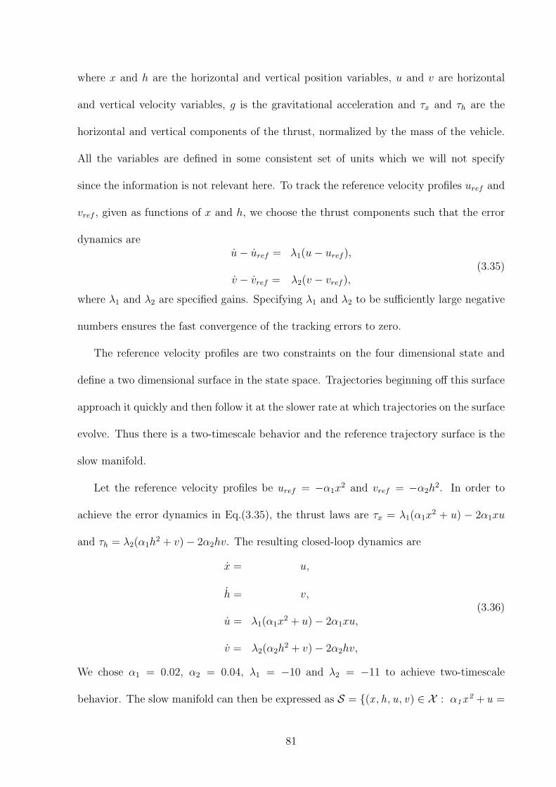
where x and h are the horizontal and vertical position variables, u and v are horizontal
and vertical velocity variables, g is the gravitational acceleration and τx and τh are the
horizontal and vertical components of the thrust, normalized by the mass of the vehicle.
All the variables are defined in some consistent set of units which we will not specify
since the information is not relevant here. To track the reference velocity profiles uref and
vref , given as functions of x and h, we choose the thrust components such that the error
dynamics areu− uref = λ1(u− uref ),
v − vref = λ2(v − vref ),(3.35)
where λ1 and λ2 are specified gains. Specifying λ1 and λ2 to be sufficiently large negative
numbers ensures the fast convergence of the tracking errors to zero.
The reference velocity profiles are two constraints on the four dimensional state and
define a two dimensional surface in the state space. Trajectories beginning off this surface
approach it quickly and then follow it at the slower rate at which trajectories on the surface
evolve. Thus there is a two-timescale behavior and the reference trajectory surface is the
slow manifold.
Let the reference velocity profiles be uref = −α1x2 and vref = −α2h
2. In order to
achieve the error dynamics in Eq.(3.35), the thrust laws are τx = λ1(α1x2 + u) − 2α1xu
and τh = λ2(α1h2 + v)− 2α2hv. The resulting closed-loop dynamics are
x = u,
h = v,
u = λ1(α1x2 + u)− 2α1xu,
v = λ2(α2h2 + v)− 2α2hv,
(3.36)
We chose α1 = 0.02, α2 = 0.04, λ1 = −10 and λ2 = −11 to achieve two-timescale
behavior. The slow manifold can then be expressed as S = (x , h, u, v) ∈ X : α1x2 +u =
81

0 , α2h2 + v = 0. Figure (3.6) shows the projections of some representative trajectories
onto the x− u and h− v planes.
10 15 20 25 30−25
−20
−15
−10
−5
0
x
u
5 10 15 20 25 30−50
−40
−30
−20
−10
0
h
v
ILDM
LVBM
ILDM
LVBM
actual slow manifold
actual slow manifold
Figure 3.6: Planar slices of the state portrait for nonlinear system, Eq. (3.34), showing actualslow manifold and approximate slow manifold points determined from orthogonality conditionsusing eigenvectors (ILDM method) and using Lyapunov vectors (LVM).
Now we will demonstrate, using Lyapunov exponents and vectors, the diagnosis of two-
timescales and the determination of the slow manifold. The bounded state space region to
be analyzed is chosen to be X = (x, h, u, v) ∈ R4 s.t. 2 ≤ x ≤ 40, 2 ≤ h ≤ 40, −32 ≤ u ≤
−1 and−64 ≤ v ≤ −2, a region containing the relevant portion of the reference trajectory
and the range of expected state perturbations. The characteristic time Tc is 6 seconds. By
calculating the Lyapunov exponents at several points in X for various averaging times, we
diagnose that X is a two-timescale set with µf = 11, µs = 3, Tmin = 0.3, nfc = 2, ns = 2,
and nfe = 0. An averaging time of 1 second is sufficient for accurate computation of
the Lyapunov vectors, since the gap is ∆µ = 8. Figure (3.7) shows the forward and back-
ward Lyapunov exponents with 1 second averaging time for points on the slow manifold S.
Because nfc = 2, ns = 2, and nfe = 0, the slow manifold, if present, is two-dimensional
82

5 10 15 20 25 300
2
4
6
8
10
12
14
16backward time Lyapunov exponents with T=1sec.
x
5 10 15 20 25 30 35 40
−10
−8
−6
−4
−2
forward time Lyapunov exponents with T=1 sec.
x
Figure 3.7: Forward and backward Lyapunov exponents versus x for T=1 sec. in slow manifolddetermination in powered descent dynamics example
and attracting. The slow subspace Es(T, ~x) = L−nfc(T, ~x) = spanl−3 (T, ~x), l−4 (T, ~x)
and using Proposition (3.5.2), we have [Es(T, ~x)]⊥ = spanl−1 (T, ~x), l−2 (T, ~x), where
~x = (x, h, y, v)T . For each value of (x, h) consistent with X , the corresponding u and
v values for the point on the slow manifold are obtained by solving the following algebraic
equations< f(~x), l−1 (T, ~x) > = 0,
< f(~x), l−2 (T, ~x) > = 0.(3.37)
Figure (3.6) shows the actual slow manifold, the slow manifold computed using the
Lyapunov vectors with 1 second averaging time, and the slow manifold computed by the
ILDM method, in both the x − u plane (h = v = 0) and h − v plane (x = u = 0). The
Lyapunov vector method identifies the points on the slow manifold more accurately than
the ILDM method.
83

3.8 Slow Manifold Determination in Van der Pol Os-
cillator Dynamics
In this section the widely known Van der Pol equations are examined and the orthogonality
conditions using the eigenvectors and Lyapunov vectors are used in order to compute the
slow manifold. Consider the Van der Pol equation given in the singularly perturbed form
x1 = x2,
εx2 = −x1 + x2 − 13x3
2.(3.38)
where ε = 0.1. The dynamics in Eq. (3.38) have an unstable equilibrium point at the origin
and -it is known that- a stable limit cycle [49]. The trajectories starting from different
initial conditions are shown in Fig. (3.8).
−3 −2 −1 0 1 2 3−3
−2
−1
0
1
2
3
x1
x2
B1i
B1f
B2i
B2f
Figure 3.8: Phase portrait of the Van der Pol oscillator for ε = 0.1.
Depending on the initial condition, all trajectories are attracted to a branch of the
slow manifold, either to B1i − B1f branch or to B2i − B2f branch. Then, the trajectory
slides along the slow manifold and is attracted to the other branch after a certain point.
For details of the dynamics within the context of the singular perturbation theory see [49].
Our aim is to concentrate on the rectangular region in Fig. (3.8) and compute the part of
84

the slow manifold in that region. The compact X region is X = (x1, x2) ∈ R2 : − 2 ≤
x1 ≤ 0.5 and 1 ≤ x2 ≤ 3.
The methodology for diagnosing a two-timescale set is applied to the region X . Figure
(3.9) shows the forward and backward finite time Lyapunov exponents computed at several
points along a trajectory for an averaging time T = 0.2 versus the x1 components of the
points.
−1.6 −1.4 −1.2 −1 −0.8 −0.6 −0.4 −0.2 0−40
−30
−20
−10
0
10
x1
−1.6 −1.4 −1.2 −1 −0.8 −0.6 −0.4 −0.2 0−10
0
10
20
30
40
50
x1
µi+(0.2,x),i=1,2
µi−(0.2,x), i=1,2
Figure 3.9: Forward and backward Lyapunov exponents for the Van der Pol dynamics versus x1
for T = 0.2.
For the finite time Lyapunov exponents with the averaging time T = 0.2 there exists
a gap of around 20. At point [−1, 2.1] the finite time forward and backward Lyapunov
exponents and the angles between the finite time Lyapunov vectors and the horizontal
axis are illustrated in Fig. (3.10). From Fig. (3.10) the gap exists for all averaging
times T ∈ (0, 0.2] and the Lyapunov vectors converge. This convergence behavior is
representative of that at all points in X . Thus, the closed set X is a two-timescale set
85

with a uniform spectral gap ∆µ = 18, µf = 19, µs = 1, nfc = 1 and ns = 1. Although Tc
is about 0.8, an averaging time of 0.2 is appropriate for the convergence of the directions.
Tmin can be taken zero in this case.
−0.2 −0.15 −0.1 −0.05 0−10
0
10
20
30
40
Averaging Time, T−0.2 −0.15 −0.1 −0.05 00
20
40
60
80
100
Averaging Time, T
de
gre
e
0 0.05 0.1 0.15 0.2−40
−30
−20
−10
0
10
Averaging Time, T0 0.05 0.1 0.15 0.2
0
20
40
60
80
100
Averaging Time, T
de
gre
e ∠ (l+1(T,x), horizontal axis)
∠ (l+2(T,x), horizontal axis)
∠ (l−1(T,x), horizontal axis)
∠ (l−2(T,x), horizontal axis)
µ+i(T,x), i=1,2
µ−i(T,x), i=1,2
Figure 3.10: Forward and backward Lyapunov exponents for the Van der Pol dynamics versusthe averaging time at point (−1; 2.1).
Because nfc = 1, ns = 1, and nfe = 0, the slow manifold, if exists, is one-dimensional
and attracting. The slow subspace is spanned by l−2 (T, x). Using Proposition (3.5.2),
[Es(T, x)]⊥ = spanl−1 (T, x). For each value of x1 consistent with X , the corresponding
values for the point on the slow manifold are obtained by solving the following algebraic
equation
〈f(x), l−1 (T, x)〉 = 0. (3.39)
86

The slow manifold is computed by solving the following equation which is the orthogonality
condition of the ILDM method
〈f(x), ve(x)〉 = 0, (3.40)
where ve(x) is the eigenvector of ∂f(x)∂x
at the point x corresponding to the eigenvalue of
∂f(x)∂x
with smaller absolute value.
Figure (3.11) shows the slow manifold computed using the Lyapunov vectors with
T = 0.2, the slow manifold computed by the ILDM method and some representative
trajectories in region X . The Lyapunov vector method identifies the points on the slow
manifold more accurately than the ILDM method. The accuracy of the computation
using the Lyapunov vectors can be further improved by increasing the averaging time.
Note that an averaging time T = 0.2 is used in the computation of the slow manifold
although Tc = 0.8.
3.9 Slow Manifold Determination in a 3 Species Ki-
netics Problem
In this section, we will demonstrate the slow manifold determination in a 3 species kinetics
problem. The same problem is used in [50]. The dynamics under consideration is given as
x1
x2
x3
=
1
ε
−5x1 − x1x2 + εx2x3 + 5x2
2 + x3 − εx1
10x1 − x1x2 − εx2x3 − 10x22 + x3 + εx1
x1x2 − εx2x3 − x3 + εx1
, (3.41)
where ε = 0.01. For this system, the compact region X = x1, x2, x3 ∈ R3 : 0 ≤
x1, x2, x3 ≤ 1 is chosen. The finite time Lyapunov exponents at the point (0.6, 0.8, 0.5)
are shown in Fig. (3.12). It can be seen in Fig. (3.12) that there are spectral gaps of
around 1800 and 200 between µ+1 (T, x) and µ+
2 (T, x) and between µ+2 (T, x) and µ+
3 (T, x)
respectively. Because of the spectral gap between µ+1 (T, x) and µ+
2 (T, x), there should
be a 2 dimensional manifold toward which all the trajectories off that manifold should
87

−2 −1.5 −1 −0.5 0 0.51
1.2
1.4
1.6
1.8
2
2.2
2.4
2.6
2.8
3
x1
x2
+ ILDM* LVM
Figure 3.11: The slow manifold computed using the orthogonality conditions with the Lyapunovvectors and the eigenvectors of the Jacobian matrix.
converge. Besides this 2 dimensional manifold, due to the spectral gap between µ+2 (T, x)
and µ+3 (T, x), there should be a 1 dimensional submanifold of the 2 dimensional manifold
to which all the trajectories eventually converge.
The 2 dimensional manifold can be computed by using nfc = 1 and ns = 2. In this
case, the partial equilibrium conditions become
〈f(x), l−1 (T, x)〉 = 0. (3.42)
On the other hand, the 1 dimensional manifold can be computed by using nfc = 2 and
ns = 1. In this case, the constraints to be satisfied at the points on the 1 dimensional
88
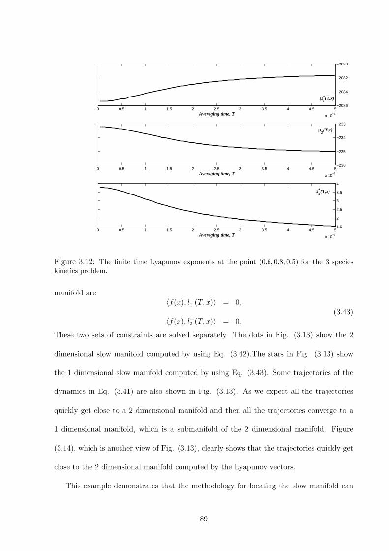
0 0.5 1 1.5 2 2.5 3 3.5 4 4.5 5
x 10−3
−2086
−2084
−2082
−2080
Averaging time, T
µ+1(T,x)
0 0.5 1 1.5 2 2.5 3 3.5 4 4.5 5
x 10−3
−236
−235
−234
−233
Averaging time, T
µ+2(T,x)
0 0.5 1 1.5 2 2.5 3 3.5 4 4.5 5
x 10−3
1.5
2
2.5
3
3.5
4
Averaging time, T
µ+3(T,x)
Figure 3.12: The finite time Lyapunov exponents at the point (0.6, 0.8, 0.5) for the 3 specieskinetics problem.
manifold are〈f(x), l−1 (T, x)〉 = 0,
〈f(x), l−2 (T, x)〉 = 0.(3.43)
These two sets of constraints are solved separately. The dots in Fig. (3.13) show the 2
dimensional slow manifold computed by using Eq. (3.42).The stars in Fig. (3.13) show
the 1 dimensional slow manifold computed by using Eq. (3.43). Some trajectories of the
dynamics in Eq. (3.41) are also shown in Fig. (3.13). As we expect all the trajectories
quickly get close to a 2 dimensional manifold and then all the trajectories converge to a
1 dimensional manifold, which is a submanifold of the 2 dimensional manifold. Figure
(3.14), which is another view of Fig. (3.13), clearly shows that the trajectories quickly get
close to the 2 dimensional manifold computed by the Lyapunov vectors.
This example demonstrates that the methodology for locating the slow manifold can
89

0.350.4
0.450.5
0.550.6
0.650.7
0.750.8
0.40.45
0.50.55
0.60.65
0.70.75
0.80.85
0.9
0.5
0.6
0.7
0.8
0.9
x
y
z
Figure 3.13: Phase portrait, 1 dimensional and 2 dimensional slow manifolds computed by usingthe constraints in Eqs. (3.42) and (3.43).
be used in the existence of multiple spectral gaps. The procedure is a repetition of the
method explained for a single spectral gap. By adjusting the constants nfc, ns, and nfe,
the slow manifolds of different dimensions can be computed. Note that the accuracy of
the slow manifold computed is dependent on the associated spectral gap.
90
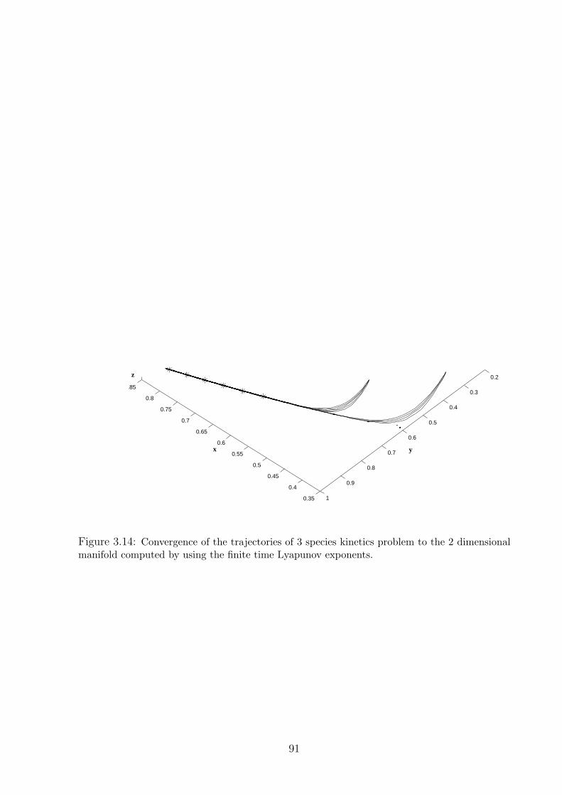
0.35
0.4
0.45
0.5
0.55
0.6
0.65
0.7
0.75
0.8
0.85
0.2
0.3
0.4
0.5
0.6
0.7
0.8
0.9
1
z
x y
Figure 3.14: Convergence of the trajectories of 3 species kinetics problem to the 2 dimensionalmanifold computed by using the finite time Lyapunov exponents.
91

Chapter 4
Lyapunov Vector Dichotomic BasisMethod for Solving Hyper-SensitiveOptimal Control Problems
4.1 Introduction to the problem and literature
In general the methods for solving optimal control problems are classified as direct methods
and indirect methods. Direct methods parametrize the control and/or state and cast
the optimal control problem as a nonlinear programming problem with dynamical and
boundary constraints. Indirect methods are based on the first-order optimality conditions
and solve the associated Hamiltonian boundary-value problem (HBVP).
HBVPs are hard to solve because of the ill-conditioning due to the sensitive depen-
dence on the unknown initial conditions. Hamiltonian systems have the volume preserving
feature, i.e., if a bounded, open set of initial conditions are propagated according to the
Hamiltonian vector field, the set of the propagated points occupy the same volume as the
initial set. If the set contracts in some directions, it expands in some other directions. This
means there exists an equal number of stable and unstable directions in the Hamiltonian
vector field. An error in the unknown initial conditions grows exponentially in certain
directions with the time span of interest.
An optimal control problem and its corresponding HBVP are called completely hyper-
92

sensitive, if the time interval of interest is very long relative to the minimum rate of
contraction and expansion of the Hamiltonian system in the neighborhood of the optimal
solutions to the HBVP [4, 5]. If the expansion and the contraction are fast only in some
directions, it is called partially hyper-sensitive. Achieving a specified accuracy on the
terminal boundary conditions requires the initial conditions in the fast expanding directions
to be very accurate or even to exceed the available precision. The indirect shooting method
can be modified using multiple shooting nodes, denser in the boundary-layers, to handle
the hyper-sensitivity. Although multiple shooting method may be capable of producing
solutions with the required accuracy, it does not provide any information regarding the
structure of the solution on the Hamiltonian state space.
The solution of a hyper-sensitive HBVP is composed of a short initial boundary-layer
segment, a long intermediate segment dominated by the slow behavior and a short termi-
nal boundary-layer segment. Besides the dynamics themselves, the intermediate segment
is determined primarily by the cost functional, whereas the boundary-layers connect the
intermediate segment to the boundary conditions. The initial boundary-layer trajectory
approaches the intermediate segment in forward time and the terminal boundary layer ap-
proaches the intermediate segment in backward time. For the completely hyper-sensitive
HBVP, the slow segment is the equilibrium solution. The composite solution to the par-
tially hypersensitive problems can be constructed by the analytical singular perturbation
method in the special case, where the two-timescale Hamiltonian dynamics are given in
the standard singularly perturbed form [34]. It decomposes the system into fast and slow
subsystems and solves the reduced-order problems. The solution to the HBVP is then con-
structed by matching the asymptotic expansions of the solutions for the boundary-layer
segments and the intermediate segment [2, 38]. Unfortunately, a systematic procedure for
93
transforming a two-timescale Hamiltonian system in general form to standard singularly
perturbed form is not available. This restricts the applicability of the singular perturbation
method.
For completely hyper-sensitive optimal control problems in general form, an indirect
solution method based on the underlying geometric structure of the trajectories of the
Hamiltonian system in the state-costate space has been introduced [4, 5]. The method
uses a dichotomic transformation to decouple the contracting and expanding behavior.
The solution to the HBVP is constructed by forward integration of the contracting part of
the dynamics and backward integration of the expanding part of the dynamics. The use
of dichotomic transformations for the solution of linear boundary-value problems is well
known in the numerical analysis literature [23]. Chow [51] used dichotomic transformations
for nonlinear two-timescale HBVPs in standard form with linear boundary layer dynamics.
Rao and Mease [4, 5] used the geometric characterization of two-timescale systems by
Fenichel [33] and the stable and unstable sub-bundles of Sacker and Sell [52] to extend the
use of dichotomic transformations to nonlinear HBVPs.
In [4, 5] the basis vectors to construct approximate dichotomic transformations are
local eigenvectors of the Jacobian of the Hamiltonian vector field. It is well known that
the eigenvectors do not provide the correct structure of the linear time-varying system
which results when the nonlinear Hamiltonian system is linearized around a reference
trajectory. Thus, an iterative algorithm was used to approximate the initial and terminal
boundary-layers. In [11, 12] it is shown that Lyapunov vectors give accurate information on
the geometry of the underlying linearized time-varying systems of the nonlinear systems.
In this work, we propose to use appropriate Lyapunov vectors to construct the dichotomic
basis, and demonstrate that the finite averaging time Lyapunov vectors can be used to
94

approximate the Lyapunov vectors for this purpose.
4.2 Hamiltonian Boundary Value Problem
Consider the following optimal control problem of finding a piecewise continuous control
u(t) ∈ Rm on [0, tf ] that minimizes the scalar cost
J =∫ tf
0L(s, u)dt (4.1)
subject to system dynamics
s = f(s, u) (4.2)
and boundary conditionss(0) = s0
s(tf ) = sf
(4.3)
where s(t) ∈ Rn is the state.
The first-order necessary optimality conditions lead to a HBVP which is composed of
the Hamiltonian differential equations
s = H∗λ
T
λ = −H∗s
T
(4.4)
with the boundary conditions (4.3), where λ(t) ∈ Rn is the costate,
H∗(s, λ) = L(s, u∗(s, λ)) + λT f(s, u∗(s, λ)) (4.5)
is the Hamiltonian evaluated for the optimal control
u∗(s, λ) = arg minu
H(s, λ, u), (4.6)
and Hλ and Hs are partial derivatives with respect to the subscripted variable. We assume
that H is a continuously differentiable function of s and λ.
95

The vector field of Eq.(4.4) is called Hamiltonian vector field. Hamiltonian vector fields
are divergence-free, i.e.,
div
HTλ
−HTs
=
∂
∂s
∂H
∂λ− ∂
∂λ
∂H
∂s= 0. (4.7)
By Liouville’s theorem [53], the Hamiltonian flow is volume-preserving, and for every
direction along which the flow is contracting, there exists a corresponding direction along
which the flow is expanding at the same rate as the contracting behavior. If there is a full
set of boundary conditions at the initial or final time, the the vector field can be integrated
and the solution trajectory can be obtained. However, for the two-point boundary value
problems, with some boundary conditions given at the initial time and some at the final
time, the error in the solution will grow as a consequence of the error in the unknown
boundary conditions because of the expanding directions in the Hamiltonian vector field.
The s-space and the (s, λ)-space are called the state space and the phase space, re-
spectively. Our attention is on the HBVP, its solution, and the structure of this solution
trajectory and its neighbors in the phase space.
4.3 Supporting Theory and Terminology
In order to simplify the notation, x = (s, λ), and
x =
(s
λ
)= f(x) = (Hλ(x),−Hs(x)) (4.8)
are sometimes used. P represents the Euclidean phase space R2n. The tangent space
at a point x of the phase space P is the space of the tangent vectors, (δs, δλ), of all
possible continuously differentiable trajectories through x. The tangent space at x ∈ P
is a linear vector space isomorphic to R2n and is denoted by TxP . The tangent bundle is
TP = ∪x∈PTxP . A point in the tangent bundle is denoted by (x, v) where v = (δs, δλ)
96

is the 2n-dimensional vector in the tangent space with base point x, i.e. v ∈ TxP , and
satisfies the following differential equation
v =∂f
∂xv. (4.9)
The theory of Sacker and Sell [52] can be used to determine the contracting and ex-
panding directions of the Hamiltonian system by considering the linearized dynamics with
respect to a solution trajectory of Eq.(4.4). The Hamiltonian vector field x = f(x) on the
phase space induces a linear Hamiltonian flow on the tangent bundle. An initial point (x, v)
is mapped in time t to the point (φ(t, x), Φ(t, x)v), where v ∈ TxP and Φ(t, x)v ∈ Tφ(t,x)P ,
and φ(t, x) and Φ(t, x) are the solutions of the following initial value problems
φ = f(φ), φ(0, x) = x, (4.10)
Φ =∂f
∂x(φ)Φ, Φ(0, x) = I, (4.11)
where I is 2n× 2n identity matrix.
Definition 4.3.1 Let Y ⊂ P be a smooth, compact, connected submanifold of P, and let
Y be invariant with respect to the Hamiltonian flow x = f(x). Then, the induced linear
Hamiltonian flow on the tangent bundle TY admits an exponential dichotomy, if there
exist a projector on TY, a mapping Π : TY → T Y such that (i) Π is continuous, and (ii)
for each x ∈ Y, there is a linear projection Π(x) in TxY such that Π(x, v) = (x, Π(x)v) for
all (x, v) ∈ TY, where Π(x) has rank n on Y, and positive constants K and α such that
‖Φ(t, x)Π(x)Φ−1(τ, x)‖ ≤ Ke−α(t−τ), t ≥ τ
‖Φ(t, x)(I − Π(x))Φ−1(τ, x)‖ ≤ Ke−α(t−τ), t ≤ τ(4.12)
for all x ∈ Y. The range and null space of a projector on TY are defined as
range(Π) = R = (x, v) ∈ TY : Π(x )v = v
nullspace(Π) = N = (x, v) ∈ TY : Π(x )v = 0(4.13)
97

and are complementary sub-bundles of TY, i.e., R(x)∩N (x) = 0 and TxY = R(x )⊕N (x ),
where R(x) and N (x) denote fibers of the sub-bundles at x ∈ Y.
If the induced linear Hamiltonian flow on the tangent bundle TY admits an exponen-
tial dichotomy with the projector Π, then Π allows the splitting of TY into invariant,
complementary stable and unstable bundles
R = range(Π) = Vs = (x, v) ∈ TY : ‖Φ(t , x )v‖ → 0 as t → +∞
N = nullspace(Π) = Vu = (x, v) ∈ TY : ‖Φ(t , x )v‖ → 0 as t → −∞(4.14)
Consider a linear coordinate change (x, v) 7→ (x,wf ) on TY with v = Df (x)wf , where
wf is the new coordinate vector and Df is a nonsingular and continuously differentiable
2n×2n matrix valued function of x on Y . The columns of Df (x) are basis vectors for TxY
for each x ∈ Y . In terms of wf , the variational equation (4.9) becomes
wf = [D−1f JDf −D−1
f Df ] = Λ(x)wf , (4.15)
where J = ∂f/∂x is the local Jacobian matrix, Df is obtained by taking the Lie derivative,
in the f direction, of each element of Df , and Λ is used to denote the transformed system
matrix more concisely.
Definition 4.3.2 Concerning the exponential dichotomy for the linear flow on TY, a basis
Df is a dichotomic basis, if it satisfies the following two requirements.
1. The corresponding system matrix Λ is block-triangular of the form
Λ =
(Λs(x) Λsu(x)
0 Λu(x)
)(4.16)
for all x ∈ Y, and the matrices Λs and Λu are both (n× n) dimensional.
2. The transition matrices Φs(t, x) and Φu(t, x) corresponding to Λs and Λu, defined
such that Φs(0, x) = I and Φu(0, x) = I satisfy the inequalities
‖Φs(t, x)Φ−1s (τ, x)‖ ≤ K1‖Df (φ(τ, x)‖‖D−1
f (φ(t, x))‖e−α(t−τ), t ≥ τ
‖Φu(t, x)Φ−1u (τ, x)‖ ≤ K1‖Df (φ(τ, x)‖‖D−1
f (φ(t, x))‖e−α(t−τ), t ≤ τ(4.17)
98
where α and K1 are positive constants.
The subscripts “s” and “u” indicate the stable and unstable nature of the two subsystems.
A dichotomic basis can be split in the form
Df (x) = [Df s(x) Df u(x)], (4.18)
whereDf s(x) = [d1(x) ... dn(x)]
Df u(x) = [dn+1(x) ... d2n(x)].(4.19)
Correspondingly, the new coordinate vector splits as
wf =
(wfs
wfu
). (4.20)
A point in the stable sub-bundle Vs has the form (x, (wfs , 0)). The fiber Vs(x) of the
stable sub-bundle is given by the column span of Df s(x). Note that the stable sub-bundle
is invariant under the dynamics, since an initial point of the form (x, (wfs(0), 0)) maps
to a point (φ(t, x), (wfs(t), 0)) = (φ(t, x), (Φs(t)wfs(0), 0)) and remains in the stable sub-
bundle. In addition, it could be required that a dichotomic basis yield Λsu = 0. Then
Vu(x) would be spanned by Df u(x). But this property is not needed for our purposes.
The Hamiltonian vector field f assigns to each phase point x = (s, λ) a vector f(x) =
(Hλ(s, λ),−Hs(s, λ)) in the tangent space at that point. At each phase point, this partic-
ular tangent vector can be expressed in the dichotomic basis as
f(x) =
(HT
λ (s, λ)−HT
s (s, λ)
)= Df s(s, λ)wfs + Df u(s, λ)wfu , (4.21)
where the tangent vector coordinates wfs and wfu are determined by
wfs = hfs(s, λ) = Df†s(s, λ)f(s, λ),
wfu = hfu(s, λ) = Df†u(s, λ)f(s, λ),
(4.22)
99

where Df†s(x) ∈ Rn×2n and Df
†u(x) ∈ Rn×2n and are the first and second, respectively, n
rows of Df−1
Df−1(x) =
(Df
†s(x)
Df†u(x)
). (4.23)
An alternative to integrating Eq.(4.4) to compute the extremal for a given initial con-
dition (s0, λ0) is to integrate the system(
s
λ
)= Df s(s, λ)wfs + Df u(s, λ)wfu
(wfs
wfu
)=
(Λs(s, λ) Λsu(s, λ)
0 Λu(s, λ)
) (wfs
wfu
) (4.24)
with the initial conditions
s(0) = s0, λ(0) = λ0,
wfs(0) = hfs(s0, λ0), wfu(0) = hfu(s0, λ0).(4.25)
This alternative makes clear that a property of a dichotomic basis is for a given initial
condition on the state, s(0) = s0, the unstable component of the Hamiltonian vector field
can be suppressed at t = 0 by choosing λ(0) = λ0 such that hfu(s0, λ0) = 0; and that
the unstable component will remain suppressed, due to the lack of coupling from wfs to
wfu . In other words, we choose λ0 such that we are at a point in the phase space on the
s = s0 hyper-plane where the Hamiltonian vector field lies in the fiber Vs(s0, λ0) of the
stable sub-bundle.
Another dichotomic transformation can be obtained by changing the order of the blocks
in the transformation, Df (x), which span the fibers Vs(x) and Vu(x) of the stable and
unstable sub-bundles, respectively, as
Db(x) =(
Dbu(x) Dbs(x)). (4.26)
The dichotomic transformation, Db(x), brings the linearized system matrix into the form
Λ =
(Λu(x) Λus(x)
0 Λs(x)
)(4.27)
100

for all x ∈ Y . The transition matrices Φu(t, x) and Φs(t, x) corresponding Λu and Λs
satisfy the second property in Definition (4.3.2).
For backward integration, Λs subsystem is unstable and Λu subsystem is stable. For a
given final condition (sf , λf ), the differential equations(
s
λ
)= Dbs(s, λ)wbs + Dbu(s, λ)wbu
(wbu
wbs
)=
(Λu(s, λ) Λus(s, λ)
0 Λs(s, λ)
) (wbu
wbs
) (4.28)
with the final conditions
s(tf ) = sf , λ(tf ) = λf ,wbs(tf ) = hbs(sf , λf ), wbu(tf ) = hbu(sf , λf ).
(4.29)
can equivalently be integrated instead of integrating Eq.(4.4), where v = Db(x)wb =
Db(x)
(wbu
wbs
), hbs = Db
†s(x)f(x), hbu = Db
†u(x)f(x), and Db
−1(x) =
(Db
†u
Db†s
). For a
given final condition on the state, s(tf ) = sf , the stable component, which is unstable
under backward propagation, of the Hamiltonian vector field can be suppressed at t = tf
by choosing λ(tt) = λf such that hbs(sf , λf ) = 0; and the stable components will remain
suppressed under backward propagation, because wbs is decoupled from wbu . In other
words, λf is chosen such that the Hamiltonian vector field, f(x), lies in the fiber Vu(sf , λf )
of the unstable sub-bundle, at the final point on the s = sf hyper-plane.
4.4 Geometric Structure of the Solution to Hyper-
Sensitive Hamiltonian Boundary-Value Problem
In the phase space, the solution trajectories to a hyper–sensitive HBVP lie in a normally
hyperbolic slow invariant manifold and its transverse fast-stable and fast-unstable mani-
folds. Outside the initial and terminal boundary-layers, the solution is well approximated
by a trajectory in the slow manifold, called the reduced-order trajectory. The complete so-
lution trajectory begins slightly off the fast-stable manifold of the reduced-order trajectory
101

and follows it quickly towards the slow manifold. The trajectory then progresses slowly
along the reduced-order trajectory. Near the final time, the trajectory quickly follows the
fast-unstable manifold of the reduced-order trajectory to the final condition slightly off
the fast-unstable manifold. For the fixed boundary conditions on the state, as the final
time increases, the initial and terminal boundary-layer segments of the trajectory lie closer
and closer to the fast-stable and fast-unstable manifolds of the reduced-order trajectory,
respectively. In the degenerate case of a completely hyper-sensitive HBVP the reduced-
order trajectory is a saddle-type equilibrium point. The fast-stable and fast-unstable
manifolds become n-dimensional stable and unstable manifolds of the saddle point. The
stable and unstable eigenspaces of the linearized Hamiltonian system at the saddle point
are n-dimensional hyperplanes tangent to the stable and unstable manifolds.
The stable manifold, Ms, is invariant with respect to the Hamiltonian flow, i.e. a
trajectory that begins on the stable manifold will remain on the stable manifold as time
progresses. An equivalent requirement for invariance is that f(x) ∈ TxMs for all x ∈Ms,
which means that the trajectory through x is tangent to Ms and will thus stay on Ms.
For all x ∈ Ms, TxMs and Vs(x) are the same subspace of TxY . Thus, f(x) ∈ Vs(x) for
all x ∈ Ms. Representing f(x) in a dichotomic basis as in Eq. (4.21), points x ∈ Ms
are identified as those for which the unstable component of the Hamiltonian vector field
is zero, i.e., wfu = hfu(s, λ) = 0. This can be viewed as a partial-equilibrium condition,
partial in the sense that the vector field f needs only be zero in certain directions. It is
clear from the block triangular form of the variational equations in Eq.(4.24) that if the
unstable component is zero at some initial point, it will remain zero along the subsequent
trajectory.
Similarly, the unstable manifold, Mu, is invariant with respect to the Hamiltonian
102

flow. Therefore, f(x) ∈ TxMu and the subspaces TxMu and Vu(x) of TxY coincide for
all x ∈ Mu. Representing f(x) in a dichotomic basis as f(x) = Dbs(x)wbs + Dbu(x)wbu ,
points x ∈Mu are identified as those for which the stable component of the Hamiltonian
vector field is zero, i.e., wbs = hbs(s, λ) = 0. It is clear from the block triangular form of
the variational equations in Eq. (4.28) that if the stable component is zero at some final
point, it will remain zero under backward propagation.
4.5 Solution of Completely Hyper-Sensitive HBVPs
and Dichotomic Basis Method
Based on the geometric structure of the phase space around the solution of the hyper-
sensitive HBVPs an approximate composite solution can be given for sufficiently large
final times as
x =
xs(t), 0 ≤ t ≤ tibl
xeq(t), tibl < t < tfbl
xu(t), tfbl ≤ t ≤ tf
(4.30)
where xs is the solution to Eq. (4.4) with the initial condition xs(0) = (s0, λ0) and λ0
is chosen such that xs(0) = (s0, λ0) ∈ Vs(xeq); xu is the solution to Eq. (4.4) with final
condition xu(tf ) = (sf , λf ) and λf chosen such that xu(tf ) = (sf , λf ) ∈ Vu(xeq); and xeq is
the equilibrium solution. The final time is tf , the duration of the initial boundary-layer is
tibl, and the duration of the final boundary-layer is tf − tfbl.
The composite solution can be continuous by introducing bridging segments. Discontinu-
ities within a specified tolerance can also be allowed at the junctions.
4.5.1 Dichotomic Basis Method
In this section a method based on a given dichotomic basis to compute the initial and ter-
minal boundary-layer segments of the composite solution to the completely hyper-sensitive
103

HBVPs is explained.
Assume that a dichotomic basis Df (x), that decomposes the Hamiltonian vector field
and the associated linearized vector field as in Eq. (4.24), is given. The stable manifold
is composed of phase points for which the unstable component of the vector field is zero.
Thus, λ(0) = λ0 can be determined such that
wfu(0) = hfu(s0, λ0) = 0 (4.31)
is satisfied for the initial state s0. The initial boundary-layer solution is then computed by
integrating Eq. (4.24) to ensure that the trajectory remains on the stable manifold. The
integration is continued until the trajectory is close enough to the equilibrium, such that
‖x(tibl)− xeq‖ ≤ ε for a specified tolerance ε, to connect it to the equilibrium solution.
In order to compute the terminal boundary-layer segment, suppose that another di-
chotomic basis, Db(x), that decomposes the Hamiltonian vector field and the associated
linearized vector field as in Eq.(4.28), is known. The unstable manifold is composed of
phase points for which the stable component of the vector field is zero. Thus, λ(tf ) = λf
can be determined such that
wbs(0) = hbs(sf , λf ) = 0 (4.32)
is satisfied for the final state sf . The terminal boundary-layer solution is then computed
by integrating Eqs.(4.28) to ensure that the trajectory remains on the stable manifold.
4.6 Lyapunov Vectors as Dichotomic Basis Vectors
The linearized Hamiltonian system in Eq. (4.9) has an equal number of expanding and
decaying directions. Assuming that there is no zero Lyapunov exponent, there exist n
forward and backward Lyapunov exponents smaller than zero, namely µ+i (x) < 0, i =
104

1, ..., n and µ−i (x) < 0, i = n + 1, ..., 2n, n forward and backward Lyapunov exponents
greater than zero, namely µ+i (x) > 0, i = n + 1, ..., 2n and µ−i (x) > 0, i = 1, ..., n, for
all x ∈ Y . The subspaces Vs(x) and Vu(x) in Eq.(4.14) can be written in terms of the
subspaces L+i (x), and L−i (x) as
Vs(x) = L+n (x)
Vu(x) = L−n+1(x).(4.33)
Using this characterization of Vs(x) and Vu(x), it can be shown that there exist C > 0
and µsu > 0 such that
v ∈ Vs(x) ⇒ ‖Φ(t, x)v‖ ≤ Ce−µsut‖v‖, t > 0, ∀x ∈ Y
v ∈ Vu(x) ⇒ ‖Φ(t, x)v‖ ≤ Ceµsut‖v‖, t < 0, ∀x ∈ Y .(4.34)
As a corollary of Theorem (2.2.6), only the Lyapunov vector corresponding to the
smallest Lyapunov exponent is invariant under linear flow. It does not preserve the mu-
tual orthogonality between the Lyapunov vectors corresponding to different Lyapunov
exponents. Differential equations that govern the propagation of the Lyapunov vectors l+i
and l−i can be derived by performing a continuous Gram-Schmidt re-orthonormalization
starting with the Lyapunov vector corresponding to the smallest exponent, namely l+1
and l−n , as the Lyapunov vectors are propagated using the linear flow. The differential
equations, that can be utilized to propagate any of the Lyapunov vectors from φ(0, x) to
other points, φ(t, x), along the trajectory and preserve the orthonormality and invariance
properties, are [54]
l+i (x) = J(x)l+i (x)− (l+i (x)T J(x)l+i (x))l+i (x)
−∑i−1j=1(l
+i (x)T J(x)l+j (x) + l+j (x)T J(x)l+i (x))l+j (x)
l−i (x) = J(x)l−i (x)− (l−i (x)T J(x)l−i (x))l−i (x)
−∑2nj=i+1(l
−i (x)T J(x)l−j (x) + l+j (x)T J(x)l−i (x))l−j (x)
(4.35)
We are now in a position to show that the basis of appropriate L+ subspaces can be
used to construct a dichotomic basis defined in Definition (4.3.2).
105

Proposition 4.6.1 Let Df ∈ R2n×2n be a matrix whose columns can be partitioned as
Df (x) = [l+1 (x)...l+2n(x)], where l+i (x), i = 1, ..., 2n are the Lyapunov vectors. Then, the
columns of Df form a dichotomic basis as defined in Definition (4.3.2), i.e., Df satisfies
the properties in Definition (4.3.2).
Proof: As given in Eq.(4.33), Vs(x) = L+n (x). We know that L+
n (x) is spanned by
l+1 (x), ..., l+n (x). Thus Df s(x) can be chosen as [l+1 (x)...l+n (x)]. In this case Df u(x) =
[l+n+1(x)...l+2n(x)]. Note that the columns of Df u(x) do not span Vu(x) and this is not
required to get the block-triangular form in Eq.(4.16).
Using the first differential equation for l+i (x) in Eq.(4.35) D can be written as
Df (x) = [l+1 (x) . . . l+2n(x)] = J(x)Df (x)−Df (x)R(x), (4.36)
where R is upper-triangular and can be written as
R(x) =
l+i (x)T J(x)l+j (x) + l+j (x)T J(x)l+i (x), if i < j
l+i (x)T J(x)l+j (x) , if i = j
0 , if i > j
(4.37)
Substituting Df in Eq.(4.15)
w = [Df−1(x)J(x)Df (x)−Df
−1(x)Df (x)]w
= [Df−1(x)J(x)Df (x)−Df
−1(x)J(x)Df (x) + Df−1(x)Df (x)R(x)]w
= R(x)w,
(4.38)
the block-triangular form in Eq.(4.16) is obtained since R(x) is an upper-triangular matrix.
It is known [20] that Lyapunov transformations, T , such that T , T−1, and T are
bounded, do not change the Lyapunov exponents. All Lyapunov vectors have, by defini-
tion, unit length; thus Df is bounded. If J(x) is bounded then Df is bounded. Since Df is
an orthogonal matrix, Df−1 = Df
T . Therefore, Df−1 is bounded. Since Df is a Lyapunov
transformation, v = Jv and w = Rw have the same Lyapunov exponents.
106
The Lyaponuv vector l+i (x) is represented by (0, ..., 0, 1, 0, ..., 0)T , where i-th entry is
1, in w-coordinates. So, the Lyapunov exponents of the subsystem, Λs, are the smallest n
Lyapunov exponents, µ+1 , ..., µ+
n , of the original system and the Lyapunov exponents of the
subsystem, Λu are the other n Lyapunov exponents, µ+n+1, ..., µ
+2n, of the original system.
The bounds in the second property of Definition (4.3.2) are obtained by using the first
inequality in Eq.(4.34). 2
Another dichotomic transformation that is used for computing the terminal boundary
can be constructed by using the appropriate backward Lyapunov vectors.
Proposition 4.6.2 Let Db ∈ R2n×2n be a matrix whose columns can be partitioned as
Db(x) = [l−2n(x)...l−1 (x)], where l−i (x), i = 1, ..., 2n are the backward Lyapunov vectors.
Then, the columns of Db form a dichotomic basis as defined in Definition (4.3.2), i.e., Db
satisfies the properties in Definition (4.3.2) with the stable subsystem Λs is decoupled from
the unstable subsystem Λu as in Eq. (4.28).
The proof of Proposition (4.6.2) is based on the invariance of the subspaces L−i (x), i =
1, ..., 2n and particularly of the subspace L−n+1(x) and uses the second equation in Eq.(4.35).
Propositions (4.6.1) and (4.6.2) show that appropriate Lyapunov vectors form sets of
dichotomic basis vectors which can be utilized in the dichotomic basis method for solving
completely hyper-sensitive HBVPs. No practical method to determine Lyapunov expo-
nents and vectors emerges from the analysis because existing theory considers asymptotic
behavior using infinite time limits on an invariant subset of the phase space. On the other
hand, most optimal control problems are posed for a finite time interval and on a compact
subset that is not necessarily invariant. When the subset is not invariant, the timescales
and the associated geometric structure characteristics of the flow on the subset must be
computable on finite-time trajectory segments. In the next section, a method for extract-
107

ing the timescale information and its associated tangent space structure on a compact
non-invariant subset is presented.
4.7 Finite Time Lyapunov Vectors as Approximate
Dichotomic Basis Vectors
We define the finite averaging time approximations of the stable and unstable subspaces
by Vs(T, x) = L+n (T, x) and Vu(T, x) = L−n+1(T, x), respectively. The accuracy with which
Vs(T, x) and Vu(T, x) approximate the stable and unstable subspaces depends on the size
of the gap relative to the available averaging time. Due to the volume-preserving feature of
the Hamiltonian systems, n of the forward and backward finite time Lyapunov exponents
are positive and n of them are negative and they are symmetric around zero. Thus, for
completely hyper-sensitive HBVPs bounds denoted by positive real numbers µf and µb for
the forward and backward finite time Lyapunov exponents exist such that
For each x ∈ X , µ+n (T, x) ≤ −µf and µf ≤ µ+
n+1(T, x) for all T ∈ (Tmin, t(x)]
For each x ∈ X , µ−n (T, x) ≥ µb and µ−n+1(T, x) ≤ −µb for all T ∈ [t(x),−Tmin).(4.39)
Let ∆µ be a positive real number such that ∆µ = 2minµf , µb. Regardless of how large
this gap is, the subspaces L+n (T, x) and L−n+1(T, x) will converge to L+
n (x) and L−n+1(x),
respectively, as T → ∞. However, we require this gap to be large enough so that the
finite time subspaces approximate the infinite time subspaces with sufficient accuracy. In
analysis the condition we are looking for is
(∆µ)−1
Tc − Tmin
=(2minµf , µb)−1
Tc − Tmin
¿ 1. (4.40)
The conditions in Eq. (4.39) are illustrated in Fig. (4.1) for only one averaging time T ,
but this structure is required for all specified values of T and x.
108

Figure 4.1: Spectra of forward and backward Lyapunov exponents illustrating the spectral gap.
Now, let the Df (T, x) ∈ R2n×2n be the matrix whose columns are partitioned as
Df (T, x) = [l+1 (T, x) ... l+2n(T, x)]. (4.41)
Since the columns of Df (T, x) do not form a dichotomic basis Λ(x), defined as
Λ(x) = Df (T, x)−1J(x)Df (T, x)− Df (T, x)−1 ˙Df (T, x), (4.42)
will not be in block-triangular form. However, when the conditions in Eqs. (4.39) and
(4.40) are satisfied, the subspace spanned by the columns L+n (T, x) will approach its infinite
time limit, the span of the column vectors of L+n (x), at the rate of 1/(e∆µT − e−∆µT ).
Therefore, when the available averaging time is long enough, the finite time Lyapunov
vectors can be used to construct a transformation to approximately decouple the stable and
unstable modes in Df (T, x)−1J(x)Df (T, x)−Df (T, x)−1 ˙Df (T, x). There are two differences
between Λ(x) and Λ(x):
• (2, 1)-block of Λ(x) is not zero, i.e. the stable and unstable modes in Λ(x) are not
decoupled. However, because of the exponentially fast convergence of L+n (T, x), the
elements of (2, 1)-block of Λ(x) decays exponentially.
• Note from Eqs. (4.37) and (4.38) that Λ(x) is not only upper block diagonal but
also upper triangular. This can be interpreted as follows: The change in wi+1 is
109

independent of wi for any i = 1, ..., 2n − 1 where w = (w1, ..., w2n)T . When the
approximate dichotomic basis used the change in wn+1, ..., ...w2n is weakly dependent
on w1, ..., ...wn due to the first property. However, the dependence of the change of
wi+1 on wi for i = 1, ..., n − 1 and the dependence of the change of wj+1 on wj for
j = n+1, ..., 2n−1 may not be weak, because only the span of the column vectors of
L+n (T, x) convergence at the rate e−∆µT . The individual column vectors of L+
n (T, x)
converge at a slower rate, if they do.
A set of linearly independent vectors that approximately decouple the linearized dy-
namics is called “approximate dichotomic basis” in [5, 4]. We propose to use the finite
time Lyapunov vectors as an approximate dichotomic basis. Similarly, the transformation
Db(T, x) = [l−2n(T, x) ... l−1 (T, x)] is another approximate dichotomic transformation that
brings the original linearized dynamics into an approximately decoupled form in which the
dependence of the rate of change of the stable components on the unstable components is
weak.
4.8 Approximate Dichotomic Basis Method
In this section, the use of an approximate dichotomic basis is justified and the advantages
of using the finite time Lyapunov vectors, instead of the eigenvectors of J(x), as the
approximate dichotomic basis are explained.
In order to compute the initial boundary layer of the composite solution to the com-
pletely hyper-sensitive HBVP, let Df (x) = [Dfs(x)Dfu(x)] be an approximate dichotomic
basis, constructed from the finite time Lyapunov vectors, on X where Dfs(x) ∈ R2n×n
and Dfu(x) ∈ R2n×n. Furthermore, let D−1f (x) be written in terms of two matrices
110
D†fs
(x) ∈ Rn×2n and D†fu
(x) ∈ Rn×2n such that
D−1f (x) =
(D†
fs(x)
D†fu
(x)
)(4.43)
and let wf represent the co-ordinate vector for the basis Df with n-dimensional components
wfs and wfu
wf =
(wfs
wfu
). (4.44)
In terms of Df (x), the differential equations for x and wf are
x˙wfs
˙wfu
=
Dfs(x) Dfu(x)
Λs(x) Λsu(x)
Λus(x) Λu(x)
(wfs
wfu
), (4.45)
where
Λ =
(Λs(s) Λsu(x)
Λus(x) Λu(x)
)= D−1
f JDf − D−1f
˙Df . (4.46)
Let Γs(t, x) and Γu(t, x) be the transition matrices corresponding to Λs and Λu, respec-
tively. Because the columns of Df (x) form only an approximate dichotomic basis, in
general, the transition matrices Γs(t, x) and Γu(t, x) have both contracting and expanding
behavior along trajectory segments in X and Λus(x) 6= 0 for p ∈ X . In terms of the
dichotomic and non-dichotomic bases, the vector f(x) can be written as
f(x) = Df s(x)ws + Df u(x)wu = Dfs(x)wfs + Dfu(x)wfu . (4.47)
Suppose we attempt to place the initial point x0 on the stable manifold by choosing
λ(0) so that wfu(0) = 0. Because the basis is non-dichotomic, the calculated initial point
will not be on the stable manifold. The size of the unstable component wu is a measure
of the error. The unstable components of f(x) at the beginning and end of the initial
boundary layer are
wu(0) = Df†u(x0)Dfs(x0)wfs(0) (4.48)
111

and
wu(tibl) = Φu(tibl, x0)Df†u(x0)Dfs(x0)wfs(0) (4.49)
In terms of the Lyapunov vectors and finite time Lyapunov vectors D†fs
(x), D†fu
(x),
D†fs
(T, x), and D†fu
(T, x) are written as
Df†s(x) =
l+1 (x)T
...l+n (x)T
, Df
†u(x) =
l+n+1(x)T
...l+2n(x)T
D†fs
(T, x) =
l+1 (T, x)T
...l+n (T, x)T
, D†
fu(T, x) =
l+n+1(T, x)T
...l+2n(T, x)T
(4.50)
by the mutual orthogonality of the Lyapunov vectors. Note that Df (T, x) is the approx-
imate dichotomic basis composed of the finite time Lyapunov vectors with an averaging
time T.
Df†u(x0)Dfs(T, x0) ∈ Rn×n and can be written as
[D†fu
(x0)Dfs(T, x0)]ij = l+i+n(x0)T l+j (T, x0). (4.51)
Any finite time Lyapunov vector can be written in terms of the infinite time Lyapunov
vectors because they form a basis for Rn×n
l+j (T, x0) =n∑
k=1
ckl+k (x0). (4.52)
By the convergence of the subspaces spanned by the Lyapunov vectors, |ck| ≤ |ak|/(e∆µT −
e−∆µT ), for k = n+1, ..., 2n where |ak| ≤ 1 due to the unit length property of the Lyapunov
vectors. Thus, each entry of Df†u(x0)Dfs(T, x0) is bounded by aij/(e
∆µT − e−∆µT ) where
|aij| ≤ 1.
The norm of wfu(tibl) can be bounded by
‖wfu(tibl)‖ ≤ ‖Φu(tibl, x0)‖‖Df†u(x0)Dfs(T, x0)‖‖wfs(0)‖, (4.53)
112

where ‖Γu(tibl, x0)‖ and ‖Df†u(x0)Dfs(T, x0)‖ denote the matrix norms induced by the
vector norm. Note that ‖Df†u(x0)Dfs(T, x0)‖ determines the size of wu and is a measure
of how well the basis Df approximates the dichotomic basis Df at point x0, because
‖Df†u(x0)Df s(T, x0)‖ = 0. In general ‖Γu(t, x0)‖ is exponentially increasing with t; thus,
the size of tibl relative to the rate of growth determines how small ‖Df†u(x0)Dfs(T, x0)‖
must be to achieve a prescribed level of accuracy. The key benefit of the composite
approximation approach is that error growth, an inherent feature of numerically integrating
a Hamiltonian system, is only taking place over the time interval tibl , which is much smaller
than tf . The factor ‖Df†u(x0)Dfs(T, x0)‖ provides additional attenuation of the growing
component of the solution since it is bounded by
‖Df†u(x0)Dfs(T, x0)‖ ≤ n|amax|/(e∆µT − e−∆µT ), (4.54)
where |amax| = maxi,j |aij| ≤ 1, using the definition of the Frobenius norm,
‖Df†u(x0)Dfs(T, x0)‖F ≤ n|amax|/(e∆µT − e−∆µT ), (4.55)
and the relation ‖A‖ ≤ ‖A‖F for any matrix A [55].
Another way to attenuate the error growth is re-initialization of the propagation along
the trajectory. Let [0, tibl] be subdivided into intervals [tk−1, tk], k = 1, ..., r, where t0 = 0
and tr = tibl. By using D†fu
(T, x(tk−1))f(x(tk−1)) = wfu(tk−1) = 0, k = 1, ..., r, the new
co-state corresponding to the current state can be found. This changes the costate such
that (x(tk−1, λ(tk−1)) is closer to the stable manifold. The trajectory may be discontinuous
in λ. Re-initialization of the propagation requires re-calculation of the Lyapunov vectors
and solving the algebraic equation D†fu
(T, x(tk−1))f(x(tk−1)) = wfu(tk−1) = 0. However, it
decreases the error accumulation and increases the accuracy of the method. Note that by
estimating ‖Φu(tk− tk−1, x(tk−1))‖ by the maximum singular value of Φ(tk− tk−1, x(tk−1)),
113

σ, e(σ−∆µ)(tk−tk−1) ≤ ε can be used as a measure of the accuracy level for some desired ε.
An analogous procedure can be used to compute the terminal boundary layer by
backward integrating from the final conditions and using the approximate dichotomic
transformation Db(x) = [l−2n(T, x) ...l−1 (T, x)], which can be decomposed as Db(x) =
[Dbu(x)Dbs(x)], where Dbu = [l−2n(T, x) ...l−n+1(T, x)] and Dbs = [l−n (T, x) ...l−1 (T, x)]. In
backward propagation wbs is unstable. It is suppressed by choosing λ(tf ) so that wbs(tf ) =
0. Since the basis is approximately dichotomic, the computed final point will not be on the
unstable manifold. The size of the stable component wbs is a measure of the error growth
under backward propagation. When calculating the terminal boundary layer, the method
aims to control the magnitude of wbs .
4.9 Iterative Procedure for Increasing the Accuracy
of the Approximate Dichotomic Basis Method
Rao and Mease [4, 5] developed an iterative procedure which starts with an approximate
dichotomic basis and determines the initial boundary-layer segment, xs, of the composite
solution by forward integrating
(x˙wfs
)=
(Dfs(x) Dfu(x)
Λs Λsu
) (wfs
wfu
)(4.56)
using wfu(·) as input and by backward integrating
(x˙wfu
)=
(Dfs(x) Dfu(x)
Λus Λu
) (wfs
wfu
)(4.57)
using wfs(·) as the input. However, since neither wfs nor wfu along xs is known a priori, this
procedure is repeated until the solution converges within a specified tolerance. The local
eigenvectors of J(x) are used to construct the approximate dichotomic basis. Since the
local eigenvectors of J(x) do not provide the correct stable and unstable directions, they
114

used the iterative procedure inspired by the Computational Singular Perturbations (CSP)
Method [10] which starts with the local eigenvectors of J(x) and uses successive corrections
to the eigenvectors to get the stable and unstable directions. The alternative basis vectors,
the finite time Lyapunov vectors, proposed in this paper are better approximations of the
correct stable and unstable directions. [11, 12] Our experience shows that the boundary-
layers xs and xu can be determined without using the iterative procedure developed by
Rao and Mease, when the finite time Lyapunov vectors are used and the conditions in Eqs.
(4.39) and (4.40) are satisfied.
4.10 Example: Nonlinear Spring-Mass System
In this section, we will illustrate the approximate dichotomic basis method on an optimal
control problem and compare the results with the exact solution obtained by using a
multi-purpose optimization software “GESOP” [56]. The system considered is a nonlinear
spring-mass system whose schematic is shown in Fig. (4.2). The displacement x of the
Figure 4.2: Schematic of the nonlinear spring-mass system.
mass is measured from the rest position of the spring, x = 0. The spring force is a nonlinear
115
function of x
fs(x) = −k1x− k2x3. (4.58)
The control that acts on the mass is an external force and is denoted by f(t). The equation
of motion of the mass is
mx− fs(x) = f(t). (4.59)
By using the state variables x1 = x and x2 = x, Eq. (4.59) can be written as
[x1
x2
]=
[x2
−k1x1+k2x31
m+ u
](4.60)
where u = f(t)/m.
Optimal Control Problem: The optimal control problem is to minimize the cost
functional
J =1
2
∫ tf
0
(q1x
21 + q2x
22 + ru2
)dt, (4.61)
where q1, q2, and q3 are positive constants, subject to the dynamic constraint in Eq. (4.59)
and the boundary constraints
x1(0) = x1i, x1(tf ) = x1f ,x2(0) = x2i, x2(tf ) = x2f .
(4.62)
This optimal control problem is the same one used in [4]. We use the same parameters
in order to be able to compare two methods. Therefore, k1 = 1, k2 = 1, m = 1, q1 = 1,
q2 = 1, r = 1, tf = 40, x1i = 1, x2i = 0, x1f = 0.75, and x2f = 0.
Hamiltonian Boundary Value Problem: The Hamiltonian can be written as
H =1
2
(x2
1 + x22 + u2
)+ λ1x2 + λ2
(−x1 − x3
1 + u). (4.63)
Since ∂H∂u
= 0 for the optimal control, u∗ = −λ2. Substituting this optimal control in Eq.
(4.63), the first order necessary conditions for optimality are obtained
x1 = x2,x2 − x1 − x3
1 − λ2,
λ1 = −x1 + λ2(1 + 3x21),
λ2 = −x2 − λ1
(4.64)
116
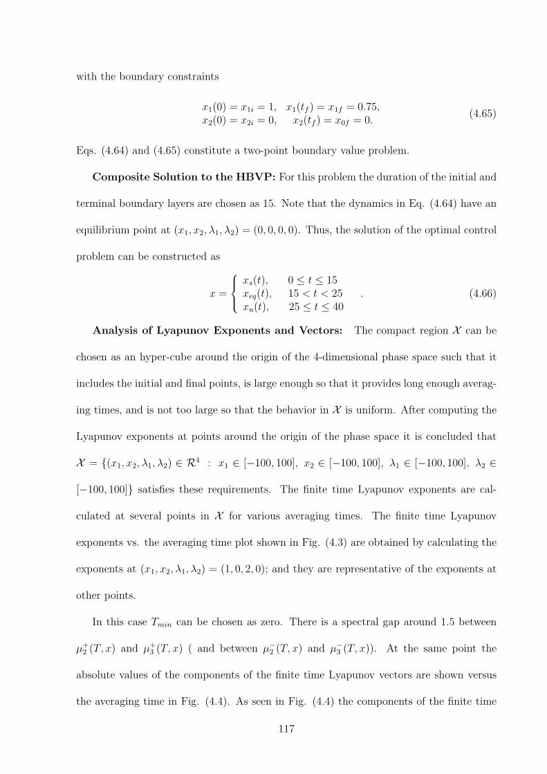
with the boundary constraints
x1(0) = x1i = 1, x1(tf ) = x1f = 0.75,x2(0) = x2i = 0, x2(tf ) = x0f = 0.
(4.65)
Eqs. (4.64) and (4.65) constitute a two-point boundary value problem.
Composite Solution to the HBVP: For this problem the duration of the initial and
terminal boundary layers are chosen as 15. Note that the dynamics in Eq. (4.64) have an
equilibrium point at (x1, x2, λ1, λ2) = (0, 0, 0, 0). Thus, the solution of the optimal control
problem can be constructed as
x =
xs(t), 0 ≤ t ≤ 15xeq(t), 15 < t < 25xu(t), 25 ≤ t ≤ 40
. (4.66)
Analysis of Lyapunov Exponents and Vectors: The compact region X can be
chosen as an hyper-cube around the origin of the 4-dimensional phase space such that it
includes the initial and final points, is large enough so that it provides long enough averag-
ing times, and is not too large so that the behavior in X is uniform. After computing the
Lyapunov exponents at points around the origin of the phase space it is concluded that
X = (x1, x2, λ1, λ2) ∈ R4 : x1 ∈ [−100, 100], x2 ∈ [−100, 100], λ1 ∈ [−100, 100], λ2 ∈
[−100, 100] satisfies these requirements. The finite time Lyapunov exponents are cal-
culated at several points in X for various averaging times. The finite time Lyapunov
exponents vs. the averaging time plot shown in Fig. (4.3) are obtained by calculating the
exponents at (x1, x2, λ1, λ2) = (1, 0, 2, 0); and they are representative of the exponents at
other points.
In this case Tmin can be chosen as zero. There is a spectral gap around 1.5 between
µ+2 (T, x) and µ+
3 (T, x) ( and between µ−2 (T, x) and µ−3 (T, x)). At the same point the
absolute values of the components of the finite time Lyapunov vectors are shown versus
the averaging time in Fig. (4.4). As seen in Fig. (4.4) the components of the finite time
117

0 0.5 1 1.5−2.5
−2
−1.5
−1
−0.5
0
0.5
1
1.5
2
2.5
averaging time, T
Finite Time Lyapunov Exponents
Figure 4.3: Finite time Lyapunov exponents vs. averaging time at x = (1, 0, 2, 0).
Lyapunov vectors do not converge within the averaging time T = 1.5. Thus, the individual
finite time Lyapunov vectors do not converge. However, in order to be able to apply the
methodology developed in the previous section, only the convergence of the subspaces
L+2 (T, x) and L−2 (T, x) is required. This is tested by solving the optimization problems
J i+(T )∗ = min
a+i1, a+
i2
‖l+i (T, x)− a+i1l
+1 (T + ∆T, x)− a+
i2l+2 (T + ∆T, x)‖, i = 1, 2 (4.67)
and
J i−(T )∗ = min
a−i1, a−i2‖l−i (T, x)− a−i1l
−1 (T + ∆T, x)− a−i2l
−2 (T + ∆T, x)‖, i = 1, 2, (4.68)
where ∆T is a pre-specified value and it is chosen as a small fraction of the averaging
time. J i+(T )∗ and J i
−(T )∗ should decrease toward zero with increasing T if the subspaces
L+2 (T, x) and L−2 (T, x) converge. For the forward time vectors, the value of J i
+(T )∗ versus
the averaging time are shown in Fig. (4.5) for i = 1, 2. Fig. (4.5) indicates that the finite
time subspace L+2 (T, x) converges, although the individual finite time vectors, l+1 (T, x) and
l+2 (T, x) in L+2 (T, x), do not from Fig. (4.4). This optimization problem is solved for other
118
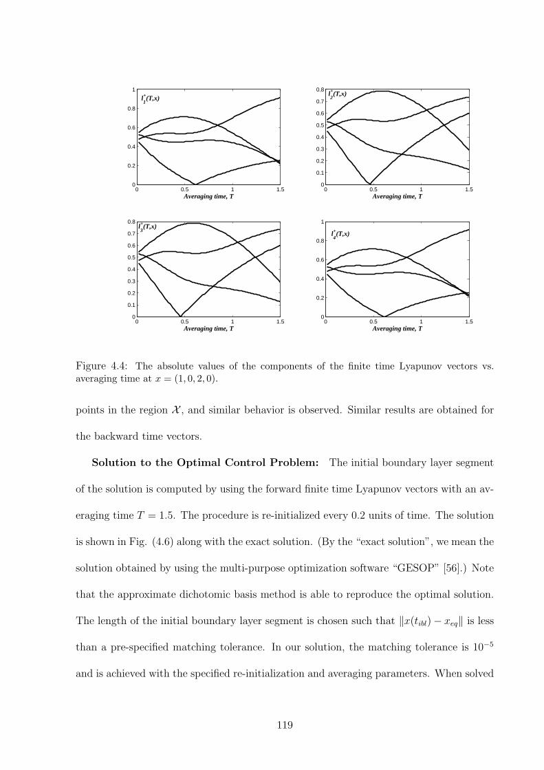
0 0.5 1 1.50
0.2
0.4
0.6
0.8
1
Averaging time, T0 0.5 1 1.5
0
0.1
0.2
0.3
0.4
0.5
0.6
0.7
0.8
Averaging time, T
0 0.5 1 1.50
0.1
0.2
0.3
0.4
0.5
0.6
0.7
0.8
Averaging time, T0 0.5 1 1.5
0
0.2
0.4
0.6
0.8
1
Averaging time, T
l+1(T,x)
l+2(T,x)
l+3(T,x)
l+4(T,x)
Figure 4.4: The absolute values of the components of the finite time Lyapunov vectors vs.averaging time at x = (1, 0, 2, 0).
points in the region X , and similar behavior is observed. Similar results are obtained for
the backward time vectors.
Solution to the Optimal Control Problem: The initial boundary layer segment
of the solution is computed by using the forward finite time Lyapunov vectors with an av-
eraging time T = 1.5. The procedure is re-initialized every 0.2 units of time. The solution
is shown in Fig. (4.6) along with the exact solution. (By the “exact solution”, we mean the
solution obtained by using the multi-purpose optimization software “GESOP” [56].) Note
that the approximate dichotomic basis method is able to reproduce the optimal solution.
The length of the initial boundary layer segment is chosen such that ‖x(tibl)− xeq‖ is less
than a pre-specified matching tolerance. In our solution, the matching tolerance is 10−5
and is achieved with the specified re-initialization and averaging parameters. When solved
119
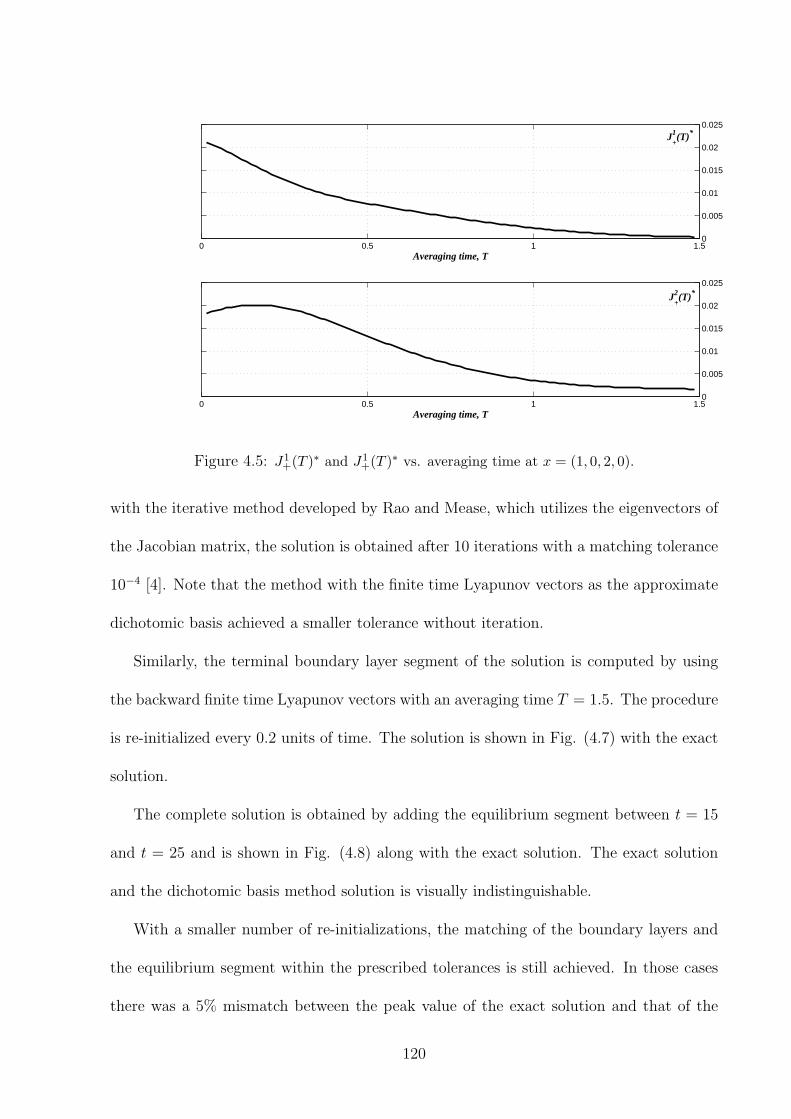
0 0.5 1 1.50
0.005
0.01
0.015
0.02
0.025
Averaging time, T
J+1(T)*
0 0.5 1 1.50
0.005
0.01
0.015
0.02
0.025
Averaging time, T
J+2(T)*
Figure 4.5: J1+(T )∗ and J1
+(T )∗ vs. averaging time at x = (1, 0, 2, 0).
with the iterative method developed by Rao and Mease, which utilizes the eigenvectors of
the Jacobian matrix, the solution is obtained after 10 iterations with a matching tolerance
10−4 [4]. Note that the method with the finite time Lyapunov vectors as the approximate
dichotomic basis achieved a smaller tolerance without iteration.
Similarly, the terminal boundary layer segment of the solution is computed by using
the backward finite time Lyapunov vectors with an averaging time T = 1.5. The procedure
is re-initialized every 0.2 units of time. The solution is shown in Fig. (4.7) with the exact
solution.
The complete solution is obtained by adding the equilibrium segment between t = 15
and t = 25 and is shown in Fig. (4.8) along with the exact solution. The exact solution
and the dichotomic basis method solution is visually indistinguishable.
With a smaller number of re-initializations, the matching of the boundary layers and
the equilibrium segment within the prescribed tolerances is still achieved. In those cases
there was a 5% mismatch between the peak value of the exact solution and that of the
120
0 5 10 15−0.2
0
0.2
0.4
0.6
0.8
1
1.2
t
x1(t)
0 5 10 15−0.8
−0.6
−0.4
−0.2
0
0.2
t
x2(t)
dichotomic basismethod solution
exact solution
dichotomic basismethod solution
exact solution
Figure 4.6: The initial boundary layer segment of the solution of the nonlinear spring-masssystem optimal control problem.
dichotomic basis method solution, although the rest of the solution was on top of each
other. This shows that the hyper-sensitivity of the system can be removed with a smaller
number of re-initialization when sub-optimal solutions are acceptable.
121

25 30 35 40−0.2
0
0.2
0.4
0.6
0.8
t
x1(t)
25 30 35 40−0.1
0
0.1
0.2
0.3
0.4
0.5
0.6
t
x2(t)
dichotomic basismethod solution
exact solution
dichotomic basismethod solution
exact solution
Figure 4.7: The terminal boundary layer segment of the solution of the nonlinear spring-masssystem optimal control problem.
0 5 10 15 20 25 30 35 40−0.5
0
0.5
1
t
x1(t)
0 5 10 15 20 25 30 35 40−1
−0.5
0
0.5
1
t
x2(t)
dichotomic basis method solution
exact solution
dichotomic basis method solution
exact solution
Figure 4.8: The composite solution of the nonlinear spring-mass system optimal control problem.
122

Chapter 5
Conclusion and Future Work
5.1 Conclusion
The purpose of this work was to identify the timescale structure of a general nonlinear
system and the associated geometric structure. The main contribution of this thesis is the
development of practical tools for understanding the timescale structure in the associated
tangent space. The tools are finite time Lyapunov exponents and vectors. In the literature,
the classical Lyapunov exponents and vectors, that are infinite time limits of the finite
time exponents and vectors in certain cases, have found extensive use in the study of
dynamical systems. However, we can only use the finite time versions in practical problems,
because only require finite averaging times are possible. The key property of the finite time
Lyapunov vectors is their exponentially fast convergence to the infinite time limits. Thus,
they provide good approximations of their infinite time limits, when there exists a long
enough averaging time relative to the spectral gap.
The motivation for this research was clarified by two simple examples in the first
chapter: the geometric structure of a nonlinear system near an equilibrium point and an
invariant manifold.
The second chapter introduced both the classical and finite time Lyapunov exponents
and vectors. The timescale decomposition in the tangent space was developed based on
123

the subspaces determined by the appropriate Lyapunov vectors. The relations between
finite time timescale information and its infinite time limit have been explained. The
invariance of the distributions in terms of the infinite time Lyapunov vectors play a cen-
tral role in proving a certain hypothesis in which the infinite time vectors were used. A
weaker invariance property, that we call “practical invariance”, was established for finite
time Lyapunov vectors and for the appropriate distributions in terms of the finite time
vectors. Some aspects about the computation of the Lyapunov exponents and vectors were
mentioned.
The third chapter was devoted to the two-timescale nonlinear dynamical systems and
the computation of the slow manifold in such systems, if the slow manifold exists. The
existing methods for computing the slow manifold were studied in order to compare the
advantages of the existing methods and the new method that is based on the finite time
Lyapunov vectors. The development of the procedure for diagnosing a possibly existing
two-timescale behavior was followed by the proposition of a new invariance based technique
for computing the slow manifold. The method was compared with the already existing
invariance based method that uses the eigenvectors of the Jacobian. The new method gave
very promising results compared to an eigenvector-based method.
The fourth chapter dealt with the geometric structure in the state-costate space for
a completely hyper-sensitive boundary value problem, that is induced by the first order
necessary conditions for optimality in a boundary-layer type optimal control problem. The
classical Lyapunov vectors were shown to be capable of identifying the geometric structure
in the tangent space. The finite time Lyapunov vectors were proposed for identifying this
structure approximately. Another invariance based method for locating the stable and
unstable manifolds of the equilibrium point was developed.
124
5.2 Future Work
The difficulty in the computation of the Lyapunov exponents and vectors makes the appli-
cation of the methods based on them challenging at this time. It is important to develop
more effective methods for computing the Lyapunov exponents and vectors.
The method for solving the boundary-layer type optimal control problems was devel-
oped for completely hyper-sensitive boundary value problems. Extending the method to
partially hyper-sensitive boundary value problems will broaden the applicability of the
method.
Finally, although a step toward model reduction in the general nonlinear systems has
been taken by understanding the timescale structure and computing the slow manifold,
these tools do not lead to a general model reduction process at the time being, unless
they are available analytically. The long term goal is to develop tools that enable model
reduction based on the timescale structure.
125

Bibliography
[1] T.J. Kaper. An introduction to geometric methods and dynamical systems theory
for singular perturbation problems. Proceedings of Symposia in Applied Mathematics,
56:85–131, 1999.
[2] R.E. O’Malley. Singular Perturbation Methods for Ordinary Differential Equations.
Applied Mathematical Sciences 89. Springer- Verlag, New York, 1989.
[3] A.E. Bryson and Y.-C. Ho. Applied Optimal Control : Optimization, Estimation, and
Control. Hemisphere Pub. Corp., Washington, 1975.
[4] A.V. Rao and K.D. Mease. Dichotomic basis approach to solving hyper-sensitive
optimal control problems. Automatica, 35:633–642, 1999.
[5] A.V. Rao and K.D. Mease. Eigenvector approximate dichotomic basis method for
solving hyper-sensitive optimal control problems. Optimal Control Applications and
Methods, 21:1–19, 2000.
[6] C. Robinson. Dynamical Systems: Stability, Symbolic Dynamics, and Chaos. CRC
Press, Boca Raton, 1994.
[7] J. Guckenheimer and P. Holmes. Nonlinear Oscillations, Dynamical Systems, and
Bifurcations of Vector Fields. Applied Mathematical Sciences 42. Springer- Verlag,
New York, 1983.
126

[8] S. Bharadwaj. Geometric structure of multiple time-scale nonlinear dynamical sys-
tems. PhD thesis, University of California, Irvine, 1999.
[9] M. Hirsch, C. Pugh, and M. Shub. Invariant Manifolds. Lecture Notes in Mathemat-
ics. Springer- Verlag, Heidelberg, 1977.
[10] S.H. Lam. Singular perturbation for stiff equations using numerical computations.
Lectures in Applied Mathematics, 24:3–19, 1986.
[11] K.D. Mease, S. Bharadwaj, and S. Iravanchy. Timescale analysis for nonlinear dy-
namical systems. Journal of Guidance, Control and Dynamics, 26(2):318–330, 2003.
[12] K.D. Mease and U. Topcu. Two-timescale nonlinear dynamics: diagnosis and slow
manifold determination. Under review.
[13] A. Isidori. Nonlinear Control Systems. Springer-Verlag, London, 3rd edition, 1995.
[14] A.M. Lyapunov. The general problem of stability of motion. International Journal
of Control, 55(3):531–773, 1992.
[15] J.A. Vastano and R.D. Moser. Short-time lyapunov exponent analysis and the transi-
tion to chaos in Taylor-Couette flow. Journal of Fluid Mechanics, 233:83–118, 1991.
[16] R.M. Samelson. Lyapunov, Floquet, and singular vectors for baroclinic waves. Non-
linear Processes in Geophysics, 8:439–448, 2001.
[17] A. Trevisan and R. Legnani. Transient error growth and local predictability: a study
in the Lorenz system. Tellus, 47A:103–117, 1995.
[18] W.E. Wiesel. Optimal pole placement in time-dependent linear systems. Journal of
Guidance, Control, and Dynamics, 18(5):995–999, 1994.
127
[19] L. Barreira and Y.B. Pesin. Lyapunov Exponents and Smooth Ergodic Theory. Uni-
versity Lecture Series Vol.23. American Mathematical Society, Providence, Rhode
Island, 2001.
[20] W. Hahn. Stability of Motion. Springer-Verlag, New York, 1967.
[21] A. Katok and B. Hasselblatt. Introduction to the Modern Theory of Dynamical Sys-
tems. Cambridge University Press, New York, 1995.
[22] S. Bharadwaj and K.D. Mease. A new invariance property of lyapunov characteristic
directions. Proceedings of the American Control Conference, 6:3800–3804, 1999.
[23] U.M. Ascher, R.M.M. Mattheij, and R.D. Russell. Numerical Solution of Boundary
Value Problems for Ordinary Differential Equations. SIAM, Philadelphia, 1995.
[24] R.A. Horn and C.R. Johnson. Matrix Analysis. Cambridge University Press, New
York, 1985.
[25] I. Goldhirsch, P.L. Sulem, and S.A. Orszag. Stability and Lyapunov stability of
dynamical systems: a differential approach and a numerical method. Physica D,
27:311–337, 1987.
[26] S. Iravanchy. Computational methods for time-scale analysis of nonlinear dynamical
systems. PhD thesis, University of California, Irvine, 2003.
[27] K. Geist, U. Parlitz, and W. Lauterborn. Comparison of different methods for com-
puting Lyapunov exponents. Progress of Theoretical Physics, 83(5):875–893, 1990.
[28] L. Dieci, R.D. Russell, and E.S. Van Vleck. On the computation of Lyapunov ex-
ponents for continuous dynamical systems. SIAM Journal on Numerical Analysis,
34(1):402–423, 1997.
128

[29] J. M. Greene and J.S. Kim. The calculation of Lyapunov spectra. Physica D, 24:213–
225, 1987.
[30] E.J. McDonald and D.J. Higham. Error analysis of QR algorithms for computing
Lyapunov exponents. Electronic Transactions on Numerical Analysis, 12:234–251,
2001.
[31] F. Christiansen and H.H. Rugh. Computing Lyapunov spectra with continuous Gram-
Schmidt orthonormalization. Nonlinearity, 10:1063–1072, 1997.
[32] J.-L. Thiffeault. Derivatives and constraints in chaotic flow: asymptotic behaviour
and a numerical method. Physica D, 172:139–161, 2002.
[33] N. Fenichel. Geometric singular perturbation theory for ordinary differential equa-
tions. Journal of Differential Equations, 31:53–98, 1979.
[34] P.V. Kokotovic, H.K. Khalil, and J. O’Reilly. Singular Perturbation Methods in Con-
trol: Analysis and Design. Academic Press, New York, 1986.
[35] D.S. Naidu and A.J. Calise. Singular perturbations and timescales in guidance and
control of aerospace systems: A survey. Journal of Guidance, Control and Dynamics,
24(6):1057–1078, 2001.
[36] A.E. Bryson, M.N. Desai, and W.C. Hoffman. Energy-state approximation in perfor-
mance optimization of supersonic aircraf. Journal of Aircraft, 6:481–488, 1969.
[37] H.J. Kelley, E.M. Cliff, and A.R. Weston. Energy state revisited. Optimal Control
Applications and Methods, 7:175–200, 1986.
[38] H.J. Kelley. Aircraft maneuver optimization by reduced-order approximation. In C.T.
Leondes, editor, Control and Dynamic Systems, pages 131–178. 1973.
129
[39] K.D. Mease. Multiple time-scales in nonlinear flight mechanics: Diagnosis and mod-
eling. Applied Mathematics and Computation, 164:627–648, 2005.
[40] S.J. Fraser. The steady state and equilibrium approximations: A geometric picture.
Journal of Chemical Physics, 88:4732–4738, 1988.
[41] M.R. Roussel and S.J. Fraser. Geometry of the steady-state approximation: pertur-
bation and accelerated convergence methods. Journal of Chemical Physics, 93:1072–
1081, 1990.
[42] U. Maas and S.B. Pope. Simplifying chemical kinetics: Intrinsic low-dimensional
manifolds in composition space. Combustion and Flame, 88(3):239–264, 1992.
[43] H. G. Kaper and T. J. Kaper. Asymptotic analysis of two reduction methods for
systems of chemical reactions. Physica D, 165:66–93, 2002.
[44] S.H. Lam and D.A. Goussis. The CSP method for simplifying kinetics. International
Journal of Chemical Kinetics, 26:461–486, 1994.
[45] K.D. Mease. Geometry of computational singular perturbations. In A.J. Krener and
D.Q. Mayne, editors, Nonlinear Control System Design, pages 855–861. Pergamon,
Oxford, UK, 1996.
[46] A. Zagaris, H.G. Kaper, and T.J. Kaper. Analysis of the computational singular
perturbation reduction method for chemical kinetics. Journal of Nonlinear Science,
14:59–91, 2004.
[47] D.A. Goussis, M. Valorina, F. Creta, and H.N. Najm. Inertial manifolds with CSP.
In K.J. Bathe, editor, Computational Fluid and Solid Mechanics, pages 1–4. Elsevier
Science, New York, 2003.
130

[48] M. J. Davis and R. T. Skodje. Geometric investigation of low-dimensional manifolds
in systems approaching equilibrium. Journal of Chemical Physics, 111(3):859–874,
1999.
[49] H.K. Khalil. Nonlinear Systems. Prentice Hall, Upper Saddle River, N.J., 3rd edition,
2002.
[50] M. Valorani, D.A. Goussis, F. Creta, and H.N. Najm. Higher order corrections in
the approximation of low dimensional manifolds and the construction of simplified
problems with the CSP method. In print, 2004.
[51] J.H. Chow. A class of singularly perturbed nonlinear, fixed endpoint control problems.
Journal of Optimization Theory and Applications, 29:231–251, 1979.
[52] R.J. Sacker and G.R. Sell. The spectrum of an invariant submanifold. Journal of
Differential Equations, 38:135–160, 1980.
[53] V.I. Arnol’d. Ordinary Differential Equations. Springer-Verlag, Berlin, 1992.
[54] W.E. Wiesel. Continuous time algorithm for Lyapunov exponents I. Physical Review
E, 47(5):3686–3691, 1993.
[55] H.G. Golub and C.F. Van Loan. Matrix Computations. The Johns Hopkins University
Press, Baltimore, 3rd edition, 1996.
[56] Institute of Flight Mechanics and Control, University of Stuttgart, Stuttgart. GESOP
Software User Manual, 2004.
[57] R. Eichhorn, S.J. Linz, and P. Hanggi. Transformation invariance of Lyapunov expo-
nents. Chaos, Solitons, and Fractals, 12:1377–1383, 2001.
131

[58] W.E. Wiesel. Modal feedback control on chaotic trajectories. Physical Review E,
49(3):1990–1996, 1994.
132

Appendix A
Lyapunov Exponents and ConstantCoordinate Transformations
It is well known that the infinite time Lyapunov exponents are invariant under coordinate
and metric transformations [11, 57]. When the norm of the transformation is bounded
above, the shift in the finite time Lyapunov exponent due to the transformation is bounded.
In case the Lyapunov exponents converge with increasing averaging time, this shift decays
with the averaging time as the averaging time tends to infinity.
Here, we develop the relation between the finite time Lyapunov exponents of two
systems that are related with a constant coordinate transformation. These relations may
be useful when the solution of a problem is obtained for scaled coordinate variables. In
this case the transformation will be a diagonal matrix.
Let x and y be two coordinates related by a constant transformation y = Tx. Let the
dynamics in x-coordinates be given by x = f(x). The linearized dynamics can be written
as δx = ∂f∂x
δx. If the integration is initiated with Φx(0, x) = I, the linearized dynamics
give δx = Φx(t, x)δx0. In y-coordinates the nonlinear dynamics is found as y = Tf(x).
The linearized dynamics are then δy = T ∂f∂x
T−1δy.
The Lyapunov exponent in x-coordinates is defined as µx(t, x, v) = 1tln ‖Φx(t, x)v‖
where v is a unit vector without the loss of generality. Then, the Lyapunov exponent in
133

y-coordinates can be defined as µy(t, y, w) = 1tln‖Φy(t,x)w‖
‖w‖ where y = Tx. The subscript of
Φ denotes the coordinate frame in which it is defined. In order to find a relation between
Lyapunov exponents in two coordinate frames let’s write the difference between them
µx(t, x, v)− µy(t, y, w) =1
tln‖Φx(t, x)v‖ ‖w‖‖Φy(t, y)w‖ . (A.1)
In order to put this equation in a more useful form we need a relation between Φx(t, x)
and Φy(t, y). By the linearized dynamics in x-coordinates δx = Φx(t, x)δx0. The same can
be done in y-coordinates to yield to δy = Φy(t, y)δy0. Using the transformation y = Tx
and correspondingly δy = Tδy we can write δx = T−1Φy(t, y)Tδx0. By comparing last
two equations for δx we can write Φy(t, y) = TΦx(t, x)T−1. If we put this in Eq. (A.1) and
use the relation w = Tv, we can write
µx(t, x, v)− µy(t, y, w) =1
tln‖Φx(t, x)v‖ ‖Tv‖‖TΦx(t, x)v‖ . (A.2)
Note that this expression requires information in x-coordinates and the transformation
matrix. Thus, it can be used for computing the finite time Lyapunov exponents in y-
coordinates.
134

Appendix B
The transients in µ vs. T plots
We have investigated what happens in the systems during the period of time that we call
Tmin and discarded in diagnosing the timescale behavior because it is not representative of
the average expansion/contraction over longer periods of time. We start by interpreting
what we see in the µ vs. T plots that appear in the analysis of each example. We will use
the 2D nonlinear example used in Chapter (3) for which we have the analytical solution.
In Fig. (B.1), µ+2 (T, 30) is the curve, which shows the finite time Lyapunov exponent
of the vector, which has the largest Lyapunov exponent for the averaging time T at point
x such that x1 = 30. It does not show the finite time Lyapunov exponent of an individual
vector. Each point on the curve corresponds to another vector. Other two curves in Fig.
(B.1) show the finite time Lyapunov exponents of the vectors l+2 (0.05, 30) and l+2 (0.1, 30).
Note that they touch the µ+2 (T, 30) curve at time 0.05 and 0.1 respectively. This is because
for the averaging time T = 0.05, l+2 (0.05, 30) is the vector that has the largest finite time
Lyapunov exponent. Thus, the point on the µ+2 (T, 30) curve at T = 0.05 corresponds
to the Lyapunov exponent of that vectors. Similarly, l+2 (0.1, 30) is the vector which is
supposed to have largest exponent for T = 0.1.
When the finite time Lyapunov exponents converge, all the finite time Lyapunov expo-
nents approach their infinite time limits as the averaging time increases. Since the infinite
135

0 0.1 0.2 0.3 0.4 0.5 0.6 0.7 0.8 0.9 1−1
−0.5
0
0.5
1
1.5
time
µ+2(T,30)
µ+(T,30,l+2(0.1,30))
µ+(T,30,l+2(0.05,30))
Figure B.1: Interpretation of µ vs. T plots.
time Lyapunov exponents are constant along the trajectories, the finite time Lyapunov
exponents at different points on the same trajectory converge to the same value. However,
they may feature different transient characteristics during the period [0, Tmin], because the
Lyapunov exponents tend to the eigenvalues of J(x)T +J(x)2
as the averaging time tends to
zero [58]. This feature is illustrated in Fig. (B.2) in which the finite time Lyapunov expo-
nent µ+2 (T, x) vs. the averaging time curves and the maximum eigenvalue of J(x)T +J(x)
2are
shown at points with different x1. Note that the µ+2 (T, x) curves are bounded from above
by the maximum eigenvalue of J(x)T +J(x)2
and µ+2 (T, x) curves approach to −1 at each x1
as the averaging time increases. Similarly, µ+2 (T, x) curves are bounded from below by
the minimum eigenvalue of J(x)T +J(x)2
. Thus, the maximum and minimum eigenvalues of
J(x)T +J(x)2
are bounds for the finite time Lyapunov exponents. But, they are tight only for
very small averaging times.
Another question that comes up during the study of the transients is what is happening
136
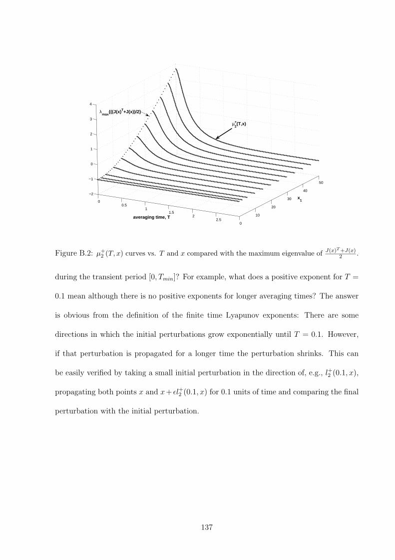
00.5
11.5
22.5
0
10
20
30
40
50
−2
−1
0
1
2
3
4
x1
averaging time, T
µ+2(T,x)
λmax
((J(x)T+J(x))/2
Figure B.2: µ+2 (T, x) curves vs. T and x compared with the maximum eigenvalue of J(x)T +J(x)
2 .
during the transient period [0, Tmin]? For example, what does a positive exponent for T =
0.1 mean although there is no positive exponents for longer averaging times? The answer
is obvious from the definition of the finite time Lyapunov exponents: There are some
directions in which the initial perturbations grow exponentially until T = 0.1. However,
if that perturbation is propagated for a longer time the perturbation shrinks. This can
be easily verified by taking a small initial perturbation in the direction of, e.g., l+2 (0.1, x),
propagating both points x and x+ εl+2 (0.1, x) for 0.1 units of time and comparing the final
perturbation with the initial perturbation.
137

Appendix C
A refinement procedure for the newbasis vectors
Although finite time Lyapunov vectors converge very quickly to infinite time vectors which
identify the correct fast and slow directions, they can be made more accurate by using a
refinement procedure without increasing the averaging times. The refinement technique
proposed is the one used in Computational Singular Perturbation (CSP) method [44, 45].
The eigenvectors are used as the starting basis in CSP method. We propose to start with
finite time Lyapunov vectors instead of eigenvectors.
For an LTV system in the singularly perturbed form
(pεq
)=
(A11 A12
A21 A22
) (pq
), p ∈ Rns
, q ∈ Rnf
(C.1)
where Aij(t) satisfy i) Re λ(A22(t)) ≤ −c1 < 0 ∀t ∈ [0, Tc], ii) Aij(t) is continuously
differentiable and bounded on [0, Tc], iii) A12(t), A21(t), A22(t) are bounded on [0, Tc]; then
there exists an ε∗ > 0 such that for all ε ∈ (0, ε∗) and there exist continuously differentiable
matrices G and H, bounded on [0, Tc], satisfying
εG = A22G− A21 − εG(A11 − A12G)
−εH = HA1 − A12 − εA2H
(C.2)
where A1 = A22 + εGA12 and A2 = A11 − A12G. Moreover, G(t) = G0(t) + O(ε) and
H(t) = H0(t) + O(ε) where G0 = A−122 A21 and H0 = A12A
−122 .
138

Then, the Lyapunov transformation(
pq
)=
(Ins − εH(t)G(t) −εH(t)
G(t) Infc+nfe
) (pq
)
= T−1(t)
(pq
) (C.3)
brings the original system into the form
˙p = [A11(t)− A12(t)G(t)]p
ε ˙q = [A22(t)− εG(t)A12(t)]q(C.4)
Then, T (t) =
(Ins εH(t)
−G(t) Infc+nfe − εG(t)H(t)
). Calculation of G(t) and H(t) in se-
ries form shows that higher-order approximations of G(t) and H(t) is a repetition of the
first-order approximations. In theory, the series expressions for G(t) and H(t) can be
used efficiently. But, in application first order approximations are more practical and
lead to T−1(t) =
(Ins − εH0G0 −εH0
G0 Infc+nfe
). This transformation, Ak+1 = AkT
−1 with
A1 is as in Eq.(C.1), will not bring the starting directions to the true fast and slow di-
rections. Successive applications of this refinement turn them to the correct directions.
This transformation holds for all ε, particularly for ε = 1 for our purposes. Although the
first assumption restricts the use of this procedure to the system having only fast stable
behavior, there is an extension of this theorem which enables it to be used for systems
with fast unstable modes [34].
Since we are also interested in Hamiltonian systems the condition on the eigenvalues
of A22(t) being less than zero is too restrictive. In [34], it is shown that the same trans-
formation can be used if A22(t) satisfies the following alternative assumption instead of
the first assumption. Alternative assumption: There exists a nonsingular continuously
differentiable matrix W (t) such that
W−1(t)A22(t)W (t) =
(D1(t) 0
0 D2(t)
)∀t ∈ [t0, tf ] (C.5)
139

where Re λ(D1(t)) ≤ −c1 and Re λ(D2(t)) ≥ c2. The assumption of the existence of
the transformation W (t) holds whenever the eigenvalues of a continuously differentiable
matrix A22(t) are bounded away from the imaginary axis.
140