lyapunov stability of linear continuous … · an overview of the lyapunov stability of lcs system...

INTERNATIONAL JOURNAL OF c© 2011 Institute for ScientificINFORMATION AND SYSTEMS SCIENCES Computing and InformationVolume 7, Number 2-3, Pages 247–268

LYAPUNOV STABILITY OF LINEAR CONTINUOUS SINGULAR

SYSTEMS: AN OVERVIEW

D.LJ. DEBELJKOVIC1 AND I.M. BUZUROVIC2

Abstract. In this article a detailed overview of Lyapunov stability of linear

continuous systems is presented. The conditions for the existence of the so-

lutions for both regular and irregular singular linear systems are introduced.

To guarantee an asymptotical stability for linear continuous singular systems

and to provide an impulse-free motion of the system, new stability conditions

are analyzed. In the control theory it is sometimes of significant interest to

preserve specific system properties under large perturbations of system model-

s. Consequently, the insensitiveness of the system properties, so-called system

robustness, is analyzed in details. Together with the system stability, the sta-

bility robustness problem is investigated. A considerable attention is focused on

the design of controllers for multivariable linear systems so that certain system

properties could be preserved under various classes of perturbations occurring

in the system.

Key Words. Continuous singular systems, Lyapunov stability, Control sys-

tems robustness

1. Introduction

For some specific classes of control systems it was noticed that the system be-haviour must be analysed in the transient process simultaneously with the systemdynamics in the stable state. Singular systems (also referred to as degenerate, de-scriptor, generalized, differential-algebraic or semi-state systems) are the ones inwhich the system dynamics was described using algebraic and differential equa-tions. Recently, many authors have been investigated the singular systems. Thecomplex nature of singular systems included many difficulties in the analytical andnumerical investigation.

So far, the singular systems have been investigated as part of the major researchtopics of control theory. During the past three decades singular systems have at-tracted much attention due to the comprehensive applications in the economics, forinstance the Leontief dynamic model [30], in the electrical and mechanical mod-els [5], [26] etc. Singular systems also arise naturally as a linear approximationof the system models, or the linear system models, in many applications such aselectrical networks, aircraft dynamics, time delay systems, chemical, thermal anddiffusion processes, large-scale systems, interconnected systems, economics, optimi-sation problems, feedback systems, robotics, biology, etc.

The discussion of singular systems was initiated in 1974 with a fundamentalarticle [7], and later was based on the work presented in [22]. Since that time,considerable progress has been made in the investigation of such systems. Thesurveys of linear singular systems were presented in [9] and [20]. The extension

Received by the editors August 1, 2011 and, in revised form, October 4, 2011.

247

248 D.LJ. DEBELJKOVIC AND I.M. BUZUROVIC

to the nonlinear singular systems was analysed in [3]. Considering the stabilityof singular systems it can be concluded that many results in sense of Lyapunovstability have been derived, as in [2] and [39].

In the previous articles the stability of linear time-varying descriptor systemswas analysed. The overall collection of the significant results in the field of stabilityof linear continuous singular systems (LCSS) was presented in a unified way. Theresults have been structured in the following way: for each stability problem, themost representative cases were given including the previous work published by theauthors of this article.

2. Basic Notations

R Real vector space

C Complex vector space

C Complex plane

I Unit matrix

F = (fij) ∈ Rn×n, real matrixFT Transpose of matrix F

F > 0 Positive definite matrix

F ≥ 0 Positive semi definite matrix

ℜ (F ) Range of matrixF

N Nilpotent matrix

N (F ) Null space (kernel) of matrix F

λ (F ) Eigenvalue of matrixF

σ() (F ) Singular values of matrix F

σ F Spectrum of matrix F

‖F‖ Euclidean matrix norm ‖F ‖=√

λmax (ATA)

FD Drazin inverse of matrix F

⇒ Follows

7→ Such that

3. Stability of Linear Continuous Singular Systems

3.1. The Stability of Linear Time Invariant Continuous Singular Sys-

tems. The general form of time invariant continuous singular control systems canbe written as:

Ex (t) = Ax (t) , x (t0) = x0(t),(1)

where x (t) ∈ Rn is a generalized state space (costate, semi-state) vector, u(t) ∈ Rl

is a control vector, E ∈ Rn×n is a possibly singular matrix, with rank E = r < n.Matrices E and A are of the appropriate dimensions and they are defined over

the field of real numbers. The system given by (1) is in a free regime and there areno external forces which act upon it. It should be noticed that the initial conditionsfor the autonomus system, as well as for the system which is in the force-actingregime, do not need to be the same. The system models represented in this formhave general representation comparing to the models in so-called normal form, e.g.when E = I. The appropriate discussion can be found in [2], [14], [15] and [16].

The complex nature of singular systems causes difficultes in the analytical andnumerical investigation, which is not the case for the systems in the normal form.

AN OVERVIEW OF THE LYAPUNOV STABILITY OF LCS SYSTEM 249

Consequently, the problems of existence, solvability, uniqueness, and smoothnesshave to be solved in the satisfactory manner. The list of problems which exist inthe theory of singular systems can be found in articles [10-12]. The survey of theupdated results for singular systems and a broad bibliography can be found in [2],[5], [6], [11], [12], [14], [20]. Two special issues of the journal Circuits, Systems and

Signal Procesing (1986, 1989) dealt with the singular systems theory.

3.2. Stability definitions. Stability plays a central role in the theory of systemsand control engineering. There are different kinds of stability problems that arisein the study of dynamic systems, such as Lyapunov stability, finite time stabilty,practical stability, technical stabilty and BIBO stability. The first part of thissection is concerned with the asymptotic stability of the equlibrium points of LCSS.The Lyapunov direct method (LDM) have been investigated in numerous researcharticles. Here, the contributions of the authors of this paper were presented togetherwith several other approaches.

Definition 3.1. System (1) is regular if there exist s ∈ C

det (sE −A) 6= 0,

[13].

Definition 3.2. Eq.(1) is exponentially stable if one can find two positive constantsα, β such that for every solution of Eq.(1), [28].

Definition 3.3. System given by Eq. (1) will be termed asymptotically stable iff,for all consistent initial conditions x0,x (t) → 0 as t → ∞, [27].

Definition 3.4. System given by Eq. (1) is denoted asasymptotically stable if allroots of det (sE −A), i.e. all finite eigenvalues of this matrix pencil, are in theopen left - half complex plane, and system under consideration is impulsive free ifthere is no x0 such that x (t)exibits discontinuous behavior in the free regime,[20].

Definition 3.5. System given by Eq. (1) is called asymptotically stable if andonly if all finite eigenvalues λi, i = 1, . . . ,n1, of the matrix pencil (λE −A) havenegative parts,[26].

Definition 3.6. The equilibrium x = 0 of system given by Eq.(1) is said to bestable if for every ε > 0, and for any t0 ∈ T , there exists aδ = δ (ε, t0) > 0, suchthat ‖x (t, t0, x0)‖ < ε holds for all t ≥ t0, wheneverx0 ∈ Wk and ‖x0‖ < δ, whereT denotes time interval such that T = [t0, +∞) , t0 ≥ 0, [8], [21].

Definition 3.7. The equilibrium x = 0 of a system given by Eq. (1) is said tobe unstable if there exist ε > 0, and t0 ∈ T , for any δ > 0, such that there existst∗ ≥ t0, for which ‖x (t∗, t0, x0)‖ ≥ ε holds, although x0 ∈ Wk and ‖x0‖ < δ, [8],[21].

Definition 3.8. The equilibrium x = 0 of a system given by Eq.(1) is saidto be attractive if for every t0 ∈ T , there exists an η = η (t0) > 0, such thatlimt→∞

x (t, t0, x0) = 0, whenever x0 ∈ Wk and ‖x0‖ < η, [8], [21].

Definition 3.9. The equilibrium x = 0 of a singular system given by Eq. (1) issaid to be asymptotically stable if it is stable and attractive, [8], [21].

Definition 3.10. System (1) is asymptotically stable if there exist positive numbersα, β satisfying, [33].

‖x (t)‖ 2 ≤ α e−β t ‖x (0)‖ 2 , t > 0.


Definition 3.5 is equivalent to limt→+∞

x (t) = 0

Lemma 3.1. The equilibrium x = 0 of a linear singular system given by Eq. (1)is asymptotically stable if and only if it is impulsive-free, and σ (E, A) ⊂ C−, [8],[21].

Lemma 3.2. The equilibrium x = 0 of a system given by Eq. (1) is asymptotically

stable if and only if it is impulsive-free, and limt→∞

x (t) = 0, [8], [21].

Due to the system structure, the system regularity quarante the existance ofthe solution of the singular control system. In that case the solution is unique.Moreover, if the consistent initial conditions are applied to the solution, then theclosed form of solutions can be established. If system (1) is regular, it is a restrictedsystem equivalent (r.s.e.) to:

x1 (t) = A1x1 (t) ,(2)

N x2 (t) = x2 (t) ,(3)

and the system is impulse free when N = 0.

3.3. Stability theorems.

Theorem 3.1. Eq. (1), with A = I, I being the identity matrix, is exponentiallystable if and only if the eigenvalues of E have non positive real parts, [28].

Theorem 3.2. Let IΩbe the matrix which represents the operator on Rn which isthe identity on Ω and the zero operator on Λ.

Eq. (1), with A = I, is stable if an n× n matrix P exist, which is the solutionof the matrix equation:

ETP + PE = −IΩ,(4)

with the following properties:P = PT ,

(5) Pq = 0, q ∈ Λ,

qTPq > 0, q 6= 0, q ∈ Ω,

where:

(6) Ω = Wk = ℵ(I − EED),

(7) Λ = ℵ(EED),

where Wk is the subspace of consistent intial conditions, [28].ℵ denotes the kernel or null space of the matrix ().

Theorem 3.3. The system given by Eq. (1) is asymptotically stable if and only if:

(1) A is invertible(2) a positive-definite, self-adjoint operator P on Rn exist, such that:(3)

ATPE + ETPA = −Q,(8)

where Q is self-adjoint and positive in the sense that, [27]:

xT (t)Qx (t) > 0forallx ∈ Wk∗\ 0 .(9)


Theorem 3.4. The system given by Eq. (1) is asymptotically stable if and only if:

(1) A is invertible and(2) a positive-definite, self-adjoint operator P exist, such that:

xT (t)(ATPE + ETPA)x(t) = −xT (t)Ix(t),

forallx ∈ Wk∗ .(10)

where Wk∗ denotes the subspace of consistent initial conditions, [27].

Theorem 3.5. Let (E,A) be regular and (E,A,C) be observable. Then (E,A) isimpulsive free and asymptotically stable if and only if a positive definite solution Pto:

ATPE + ETPA+ ETCTCE = 0,(11)

exist and if P1 andP2 are two such solutions, then ETP1E = ETP2E, [29].

Theorem 3.6. If there are symmetric matrices P , Q satisfying:

ATPE + ETPA = −Q,(12)

and if:

(13) xTETPEx > 0, x ∈ S1y1 6= 0,

xTQx ≥ 0, ∀x = S1y1,(14)

then the system described by Eq. (1) is asymptotically stable if:

(15) rank

(

sE −AST1 Q

)

= n, ∀s ∈ C,

and marginally stable if the condition given by Eq. (15) does not hold, [28].

Theorem 3.7. The equilibrium x = 0 of a system given by Eq. (1) is asymptotically

stable, if an n × n symmetric positive definite matrix P exist, such that alongthe solutions of system, given by Eq. (1), the derivative of function V (Ex) =

(Ex)T P (Ex), is a negative definite for the variates of Ex, [8], [21].

Theorem 3.8. If an (n × n) symmetric, positive definite matrix P exists, suchthat along with the solutions of system, given by Eq. (1), the derivative of the

functionV (Ex) = (Ex)T P (Ex) i.e. V (Ex) is a positive definite for all variates ofEx, then the equilibrium x = 0 of the system given by Eq. (1) is unstable, [8], [21].

Theorem 3.9. If an n× n symmetric, positive definite matrix P exists, such thatalong with the solutions of system, given by Eq. (1), the derivative of the function

V (Ex) = (Ex)TP (Ex) i.e. V (Ex) is negative semidefinite for all variates of Ex,

then the equilibrium x = 0 of the system, given by Eq. (1), is stable, [8], [21].

Theorem 3.10. Let (E,A) be regular and (E,A,C) be impulse observable andfinite dynamics detectable. Then (E,A) is stable and impulse-free if and only if asolution (P,H) to the generalized Lyapunov equations (GLE) exists, [31]:

ATP +HTA+ CTC = 0,(16)

HTE = ETP ≥ 0.(17)


Some assumptions and preliminaries are needed for further analyses. Let usconsider forced linear continuous singular systems (LCSS) represented by:

(18) Ex (t) = Ax (t) +Bu (t) , x (t0) = x0,

(19) y (t) = Cx (t) ,

Suppose that matrices E and A commute that is: EA = AE. Then a real number λexists such that (λE − I) = A., otherwise, from the property of regularity, one maymultiply Eq. (18)-(19) by (λE − A)−1 so one can obtain the system that satisfythe above assumption and keeps the stability the same as the original system. It isknown that there always exists a linear nonsingular transformation, with invertiblematrix T , such that:

(

TET−1 TAT−1)

=

diag(

E1 E2

)

diag(

A1 A2

)

,(20)

where E1 is of full rank andE2 is a nilpotent matrix, satisfying:

Eh2 6= 0, Eh+1

2 = 0, h ≥ 0.(21)

In addition, it is evident:

A1 = λE1 − I1, A2 = λE2 − I2.(22)

The system, given by Eq. (18)-(19), is (r.s.e.) to:

E1x1 (t) = A1x1 (t) +B1u (t) ,(23)

E2x2 (t) = A2x2 (t) +B2u (t) ,(24)

where xT (t) =[

xT1 (t) xT

2 (t)]

.

Lemma 3.3. The system, given by Eq. (18)-(19), is asymptotically stable if andonly if the ”slow” sub - system, Eq. (18) is asymptotically stable, [38].

Lemma 3.4. x1 6= 0 is equivalent to Eh+1x 6= 0,[38].Define Lyapunov function as

V(

Eh+1x (t))

= xT (t)(

Eh+1)T

P Eh+1x (t) ,(25)

where: P > 0, P ∈ Rn×n satisfying: V (Eh+1x) > 0 if Eh+1x 6= 0, when V (0) = 0.

From Eq. (18)-(19) and Eq. (24), bearing in mind that EA = AE, one canobtain:

(

Eh)T

ATPEh+1 +(

Eh+1)T

PAEh = −(

Eh+1)T

W Eh+1,(26)

where W > 0, W ∈ Rn×n.Eq. (26) is said to be Lyapunov equation for a system given by Eq. (18)-(19).

Denote with

deg ree det (sE −A) = rank E1 = r.(27)

Theorem 3.11. The system, given by Eq. (18)-(19), is asymptotically stable ifand only if for any matrix W > 0 , Eq. (26) has a solution P ≥ 0 with a positiveexternal exponent r, [38].

Theorem 3.12. The system, given by Eq. (18)-(19), is asymptotically stable ifand only if for any given W > 0 the Lyapunov Eq. (26) has the solution P > 0,[38].


The conclusion is the same as in the case of the well known Lyapunov stabilitytheory if E is of full rank. If matrix E is singular then there is more than onesolution. It should be noted that the results of the preceeding theorems are derivedonly for regular linear continuous singular systems.Initially, some basic statementswere presented, [19].

System (1) with a n× n matrix E is called regular if det (sE −A) 6= 0 for somes ∈ C.It can be stated that regular system (1) is:

i) Stable if all roots of det (sE −A) = 0 are in the open left-half plane;ii) Impulse free if it exhibits no impulsive behaviour.iii) Finite-dynamics detectable if (O1) holds.iv) Finite-dynamics observable if (O2) holds.v) Impulse observable if (O3) holds.vi) S-observable (Following [20], we shall say observable) of (O2) and (O3) hold.vii) C-observable if (O2) and (O4) hold where (O1)-(O4) conditions are given

by:

(O1) rank

(

sE −AC

)

= n, Re (s) ≥ 0,(28)

(O2) rank

(

sE −AC

)

= n, for all s ∈ C,(29)

(O3) rank

E A0 C0 E

= n+ rank E,(30)

(O4) rank

(

EC

)

= n.(31)

It can be concluded that C-observability implies S -observability.

Theorem 3.13. Let E, A ∈ Rn×n and C ∈ Rp×n be given by ( a Weierstrass form

of some regular system(

E, A, C)

:

E =

(

Iq 00 Λ

)

,(32)

A =

(

J 00 In−q

)

,(33)

C =(

CF C∞

)

,(34)

where Iq denotes a q × q identity matrix, J corresponds to the finite zeros of(sE −A), Λ is nilpotent (Λk = 0, Λk−1 6= 0 for some integer k > 0), and(E, A, C) is observable. Then (E,A) is stable and impulse free if and only ifthere exists a positive-definite solution P to the following Lyapunov equation:

ATPE + ETPA+ ETCTCE = 0.(35)

Moreover, if P and P ′ are two such solutions, then ETP ′E = ETPE, [19].

Theorem 3.14. Let (E,A) be regular and consider the following generalized Lya-punov equation (GLE):

ATPE + ETPA+ ETQE = 0.(36)

It can be stated:


(1) If there exist matrices P ≥ 0 and Q > 0 satisfying the GLE (36), then(E,A) is impulse free and stable;

(2) If (E,A) is impulse free and stable, then for each Q > 0 there exist P > 0

solution of GLE (36). Furthre more, ETPE ≥ 0 is unique for each Q > 0, [19].

Theorem 3.15. Let E, A ∈ Rn×n and C ∈ Rp×n be such that (O1) and (O3) ((O2)and (O3)) are satisfied. Consider also a matrix E0 ∈ Rn×(n−r) of full-column ranksuch that ETE0 = 0, where r = rank E. The following statements are equivalent:

(1) system (E,A) is regular, impulse free and stable;(2) there exists a solution P, Q ∈ Rn×n × R(n−r)×n with P ≥ 0(> 0) to the

following GLE:

ATPE + ETPA+ CTC +ATE0Q+QTET0 A = 0,(37)

(3) there exists a solution P, Q ∈ Rn×n×R(n−r)×n with ETPE ≥ 0 (ETPE ≥0

and rank(

ETPE)

= rank E) to GLE (37), [19].

Theorem 3.16. Let E, A ∈ Rn×n and C ∈ Rp×n be such that the system (E,A)is regular, impulse free and stable, and consider the following statements:

(1) The Lyapunov equation:

ATPE + ETPA+ ETCTCE = 0,(38)

has a solution P such that ETPE ≥ 0 and rank(

ETPE)

= r;

(2) The Lyapunov equation (37) has a solution P such that ETPE ≥ 0 and

rank(

ETPE)

= r.

(3) The Lyapunov equation:

ATPE + ETPA+ CTC = 0,(39)

has a solution P such that ETPE ≥ 0 and rank(

ETPE)

= r;(4) The Lyapunov equation:

(40)ETX = XTE ≥ 0 ,

ATX +XTA+ CTC = 0 ,

has a solution X such that ETX ≥ 0 and rank(

ETX)

= r.

Then: 1) (E, A, CE) is observable ((O2) and (O3) hold with C replaced by CE)if and only if i holds. 2) (E, A, C) is observable if and only if any one of thestatements ii)-iv) holds, [19].

4. Linear singular continuous irregular singular systems

In order to investigate the stability of irregular singular systems, the folowingresults can be used, [2].For this study, the linear continuous singular system is usedin the suitable canonical form, i.e.:

x1(t) = A1x1(t) +A2x2(t),(41)

0 = A3x1(t) +A4x2(t).(42)

In the following part, we examined the problem of the existence of solutions whichconverge toward the origin of the systems phase-space for regular and irregular

singular linear systems. Using a suitable nonsingular transformation, the originalsystem was transformed to its convenient form. The suggested transformation of the


system equations enables the development and easy application of Lyapunov’s directmethod (LDM) for the intended existence analysis for a subclass of the solutions.

In the case when the existence of such solutions is solved, the estimation ofthe weak domain of attraction for the system origin is obtained on the basis ofsymmetric positive definite solutions for a reduced order matrix Lyapunov equation.

The estimated weak domain of attraction consists of points of the phase space,which generates at least one solution convergent to the origin.

Let the subset of the consistent initial conditions of Eqs. (41-42) be denotedby Wk∗.Also, let us consider the manifold M ⊆ Rn×n determined by Eq. (42) asm = ℵ

( (

A3 A4

))

.For the system governed by Eq.(41-42) the set Wk∗ of theconsistent initial values is equal to the manifold M, that is Wk∗ = M.It can be seenthat the convergence of the solutions of the system given by Eq.(1) and the systemgiven by Eqs.(41-42) toward the origin is an equivalent problem, since the proposedtransformation is nonsingular. Thus, for the null solution of Eqs. (41-42), the weakdomain of attraction should be estimated.

The weak domain of attraction of the null solution x (t) = 0 of the system givenby Eq. (41-42) is defined by:

D∆=

x0 ∈ Rn : x0 ∈ M, ∃x (t,x0) , lim

t→∞||x(t,x0)|| → 0

.(43)

The term weak was used because the solutions of Eqs.(41-42) do not need to beunique, and thus for every x0 ∈ D the solutions which do not converge toward theorigin might also exist. In the previous case D = MWk∗, and the weak domainof attraction could be treated as the weak global domain of attraction. It shouldbe noted that the presented concept of the global domain of attraction differs con-siderably, with respect to the global attraction concept known for state variablesystems [2] and [14].

Now, it is possible to estimate set D . To obtain underestimate De of the setD (i.e. De ⊆ D), the LDM will be used. The further analysis will not requirethe regularity condition for matrix pencil (sE - A). For the systems in the form ofEqs.(41-42) the Lyapunov-like function can be selected as:

V (x (t)) = xT1 (t)Px1 (t) , P = PT > 0,(44)

where P was assumed to be a positive definite and real matrix.The total time derivation of V along the solutions of Eqs. (41-42) is then:

(45)V (x (t)) = xT

1 (t)(

AT1 P + PA1

)

x1 (t)+xT

1 (t)PA2x2 (t) + xT2 (t)AT

2 Px1 (t),

A brief analysis of the attraction problem shows that if Eq. (45) is negative definite,then for every x0∈Wk∗ we have ||x1(t)||→ 0 as t → ∞. Then ||x2(t)||→ 0 as t → ∞,for all solutions for which the following connection between x1(t) and x2(t) holds:

x2 (t) = Lx1 (t) , ∀t ∈ R.(46)

Since the previous is not valid for irregular singular linear systems, then the taskneeds to be reformulated. It is necessary to establish the relation (46) withoutintroducing to many addtional novel constraints to Eq. (42). To efficiently usethis fact for the analysis of the attraction problem, we introduced the followingconsideration which dictate the form of the matrix L.Let Eq. (46) hold. Assume that the rank condition:

rank(

A3 A4

)

= rankA4 = r ≤ n2,(47)


is satisfied. Then a matrix L exist, [32], being any solution of the matrix equation:

0 = A3 +A4L,(48)

where 0 is a null matrix of dimensions the same as A3. On the basis of Eq. (46), Eq.(48) and Eq. (42), it becomes evident that whenever a solution x(t) fufills Eq. (46),then it has also has to be fulfilled Eq. (42).When this holds, then all solutions of thesystem Eqs. (41)-(42), which satisfy Eq.(46), are subject to algebraic constraints

Fx(t) =

(

A3 A4

L −I

)

x(t) = 0.(49)

Assuming that V (x (t)) determined by Eq. (45) is a negative definite, the followingconclusions are important:1. The solution of Eqs. (41)-(42) has to belong to set

ℵ( (

A 3 A4

))

∩ ℵ( (

L −I))

.(50)

2. If rank F = n then evaluation of attraction domain for the null solutionis, is notpossible on the basis of the adopted approach, or more precisely, in this case theestimation of the weak domain D of attraction is a singleton:

x(t) ∈ ℵ([

A3 A4

])

: x(t) ≡ 0.(51)

3. If rank

F < n,(52)

then the estimates of the weak domain of attraction needs to be a singleton and itis estimated as

D =

x(t) ∈ Rn : x(t) ∈ ℵ

((

A3 A4

))

∩ ℵ ([L− I]) ⊆ D

(53)

Now Eq.(45) and Eq. (46) are employed to obtain:

V (x (t)) = xT1 (t)

(

(A1 +A2L)TP + P (A1 +A2L)

)

x1 (t) ,(54)

which is a negative definite with respect to x1(t) if and only if:

ΩTP + PΩ = -Q,Ω = A1 +A2L,(55)

where Q is real a symmetric positive definite matrix. Now, the following result canbe presented.

Theorem 4.1. Let the rank condition Eq. (47) hold and let rank F < n, wherethe matrix F is defined in Eq. (49). Then, the underestimate De of the weakdomain D of the attraction of the null solution of system given by Eqs. (41)-(42),is determinated by Eq. (53), providing (A1 +A2L) is a Hurwitz matrix. IfDe is nota singleton, then there are solutions of Eq. (41)-(42) different form null solution,x(t) ≡ 0, which converge toward the origin as time t → + ∞, [2].

In the following part the results for regular singular systems has been presented.

Theorem 4.2. A regular system (1) is asymptotically stable if

(56) σ (E,A) ⊂ C−

where

C− = s | s ∈ C, Re (s) < 0 , σ (E,A) ⊂ C−,(57)

stands for the field of finite poles, [33].


The previous theorem represents the basic criterion for the singular system sta-bility and for the system response evaluation. Consequently, the stability problemwas changed to an algebraic one if σ (E,A) ⊂ C− is satisfied. Moreover, the systemstability depends on coefficient matrices (E, A) of the system. The stability is asystem characteristics and reflects on system structure performances. However, theprecise pole calculation is difficult if the order of system (1)is high. In a practicalapplication, the stability criteria obtained by Lyapunov direct method are alwaysused.

The main idea of the Lyapunov method consists of introducing Lyapunov func-tion V (t, x (t)) and its derivative along the system trajectories, and consequentlydetermining the stability by using the character of V (t, x (t)) and its derivativedV (t, x (t)) /dt. The advantage of this method lies in avoiding the difficultiesof getting the system state response, and uses the character of V (t, x (t)) anddV (t, x (t)) /dt to solve the problems directly. A series of results is obtained byconstructing different Lyapunov functions.

Theorem 4.3. The system (1) is regular, impulse free and asymptotically stableif and only if there exist a matrix V satisfying the following equations:

V TA+ATV = −Q,(58)

ETV = V TE ≥ 0,(59)

for any positive definite Q, [40].

Theorem 4.4. The system (1) is regular, impulse free and asymptotically stable ifand only if there exists a unique positive semi-definite solution V to the Lyapunov

equation, [37]

ATV E + ETV A = −ETQE,(60)

satisfying

rank(

ETV E)

= rank V = r.(61)

Theorem 4.5. The system (1) is regular, impulse free and asymptotically stableif and only if the Lyapunov function, [42]

V (Ex (t)) = xT (t)ETV x (t) ,(62)

satisfying

dV (Ex (t))

dx (t)< 0,(63)

where x (t) 6= 0 and V satisfying

V E + ETV ≥ 0, rank(

ETV)

= rankE,(64)

Theorem 4.6. The system (1) is regular, impulse free and asymptotically stableif and only if there exists a symmetric solution V to [43]


satisfying:

ETV E ≥ 0, rank(

ETV E)

= rank E = r,(66)

where W is a symmetric matrix, and satisfying

ETQE ≥ 0, rank(

ETQE)

= rank E = r.(67)


Theorem 4.7. The system (1) is regular, impulse free and asymptotically stableif and only if there exists a matrix V satisfying, [23]:

V TA+ATV < 0,(68)

ETV = V TE ≥ 0.(69)

Theorems 4.3-4.7 give the sufficient and necessary condition of regular singularsystems stability, and for impulse free stability by Lyapunov direct method (LDM).LDM is different for the normal linear system, so the formulation of Lyapunovfunction for (LCSS) is not simple generalization.

Because of the complexity of LDM, there always exists constraint together withthe Lyapunov function when stability of (LCSS) was analyzed. Theorems 4.3-4.4and Theorem 4.6 were obatined by considering Lyapunov equation, and Theorem

4.5 was obtained by both Lyapunov function and Lyapunov inequality, as in The-

orem 4.7. Theorems 4.5-4.7 included a restriction of matrix rank. This kind ofrestriction was solved for low order systems, but if the order is high solution is notstreightforward. Theorems 4.3 and Theorem 4.7 are useful in these cases.

Geometry method became useful tool to solve the previous problems in controltheory. By calculating the series of ranges of a sphere according to projectivegeometry theories, [5] gave some results, which were useful in the robust controlstudies.

Theorem 4.8. The following statements are equivalent: (i) The system (1) isstable and impulse free (ii) There exist rank (LAS) = n− r and a positive definitematrix X > 0 satisfying

ET XTA+ATXE < 0,(70)

where

L ∈ Ψ ∧ S ∈ Φ.(71)

(iii) σ (E,A) ⊆ Ω, where

Φ :

L ∈ R(n−r)×n : LE = 0, rank L+ rank E = n

,(72)

E = Υ−1

(

Ir 00 −In−r

)

Θ−1,(73)

Ψ :

S ∈ Rn×(n−r) : E S = 0, rank S + rank E = n

.(74)

σ (E,A) is a spectrum of generalizes singular system. Ω stands for a six prism, [44].

Impulse free system was analyzed in Theorems 3.2-3.7, but the impulses in singu-lar systems always exists. The following results were obtained by analyzing stabilityof (LCSS) without consideration of impulse behaviour.

Theorem 4.9. A regular system (1) is asymptotically stable if and only if thereexists a solution V ≥ 0 to


satisfying

ETV E ≥ 0, rank(

ETV E)

= deg det (sE −A) ,(76)

where arbitrary Q ≥ 0 satisfies:

ETQE ≥ 0, rank(

ETQE)

= deg ree det (sE −A) ,(77)


where, [43]

EA = AE, sE −A = I.(78)

Theorem 4.10. The regular system (1) is asymptotically stable if and only if thereexists a positive-exponent solution V ≥ 0 satisfying

(

Eh)T

ATV Eh+1 +(

Eh+1)T

V AEh = −(

Eh+1)T

QEh+1,(79)

where

Q > 0, EA = AE, sE −A = I,(80)

and h is the nilpotent index of E, [38]

Theorem 4.11. The regular system (1) is asymptotically stable if and only if thereexists a solution V to Lyapunov equation

(

Eh+1)T

V = V TEh+1 ≥ 0,(81)

AT(

Eh)T

V + V TEhA = −(

Eh)T

QET ,(82)

satisfying

rank(

Eh+1)T

V = deg ree det (sE −A) = rank(

Eh+1)

.(83)

There exists a converse matrix T such that

T(

E A)

(

T−1 00 T−1

)

=

(

E1 0 A1 0

0 E2 0 A2

)

,(84)

where E1 ∈ Rg×g, A2 ∈ R(n−g)×(n−g) are invertible matrices and E2 is a nilpotentmatrix, [24].

Theorem 4.12. The regular system (1) is asymptotically stable if E−1A 1 is stable,

where E = (sE −A)−1

E, A = (sE −A)−1

A, [36].

Theorems 3.9-3.11 are all applicable to impulse systems. They became identicalas Theorem 4.6 when the system is impulse free.

4.1. The stability of linear time varying continuous singular systems.

Consider the linear continuous singular system represented by

Ex (t) = A (t)x (t) , x (t0) = x0 (t) .(85)

Theorem 4.13. Suppose that the system (85) is regular, and the following condi-tions are fulfilled at the same time:

(1) There exist constants γ > 0 and ℘ > 0 satisfying ‖A (t)‖ ≤ γ and ‖A22 (t)‖ ≥℘

(2) A22 (t) is invertible for all t ≥ 0(3) There exists a positive definite matrix

P ∈ Rr×r and constant ℓ > 0 such that

xT1 (t)

(

PW (t) +WT (t)P)

x1 (t) ≤ −ℓ ‖x1‖2 ,(86)

where

W (t) = A11 (t)−A12 (t)A−122 (t)A21 (t) ,(87)

(88) E =

(

Ir 00 0

)

, A (t) =

(

A11 (t) A12 (t)A21 (t) A22 (t)

)

,


(89) x (t) =[

xT1 (t) xT

2 (t)]T

,x1 (t) ∈ Rr, x2 (t) ∈ Rn−r

and E, A (t) are continuous functional matrices, then the time-varying singularsystem (85) is stable and impulse free, [18].

The article [4] is focused on (LDM) with A being time varying and E beingconstant.The results presented throughout Theorems 4.3-4.13 were described indetails in [25].

5. Stability Robustness Considerations

Consider the singular linear systems (SLS) represented by:

(90) Ey (t) = Ay (t) , E,A ∈ Rm×n , y (t0) = y0 ,

where y (t) ∈ Rn is the phase vector (i.e. generalized state-space vector). Thematrix E, when m = n, is possibly singular. When this is the case, then rank E =p < n, nullityE = n − p = q. If matrix E is invertible, then (1) can be written inthe normal form as:

(91) y (t) = E−1Ay (t) , y (t0) = y0 .

The behavior of the solution of (91) was documented in contemporary literature.However, this is not the situation for system (90), where m 6= n or when m = nwith detE = 0.

In the control and system theory, it is of great interest to preserve various systemproperties under large perturbations of the system model. Such perturbations ofthe model may be caused by changes in the manufacturing process of components,variations of constructive elements, or due to replacement, change of environmentalconditions, etc., [1]. The insensitiveness of the system properties is called robust-ness and it is an important field of investigation. The fact is that in many practicalsituations the parameters of system components are not exactly known. Usually,we only have some information on the intervals to which they belong. So, the ro-bustness for any system property is an important theoretical and practical question.

In the recent years considerable attention has been focused on the design ofcontrollers for multivariable linear systems so that certain system properties arepreserved under various classes of perturbations occuring in the system. Such con-trollers have been called robust controllers, and the resulting system is said to berobust in the same sense. In [29] the robustness bounds problem on unstructuredpertubations of linear continuous-time systems was solved. In [35] improved resultsfrom [29] were presented for linear perturbations with known structure. Similari-ly, the transformation method wos proposed to reduce robustness bounds conser-vatism. Recently, the authors in [34] have investigated bounds for structured andunstructured perturbations of discrete-time systems. Article [45] considered therobust stability analysis problem by state-space methods. The authors have de-rived some lower bounds on allowable perturbations that maintain the stability ofnominally stable systems with structured uncertainty. It has been shown that thosebounds were less conservative than the existing ones. New results were presented in[8] using an iterativity approach. The solutions were derived for the linear systemwith unstructured time-varying perturbations. In comparison with some existingmethods, less conservative results have been obtained.

In this article, the stability robustness problem for linear continuous singularsystems in the time domain was addressed using the Lyapunov approach. Thebounds of unstructured perturbation vector function that maintain the stability


of the nominal system with attractivity property for a subclass of solutions areobtained both for regular and irregular singular systems.

Consider an (SLS) given by (90). Introducing a suitable nonsingular transfor-mation as:

(92) Tx (t) = y (t) , T ∈ Cn×n,

a broad class of SLS (90) can be transformed to the following form:

x1 (t) = A1x1 (t) +A2x2 (t) ,(93)

0 = A3x1 (t) +A4x2 (t) ,(94)

ET =

(

I 00 0

)

, AT =

(

A1 A2

A3 A4

)

,(95)

where x (t) =[

xT1 (t) xT

2 (t)]

T ∈ Rn is a decomposed vector, with x1 ∈ Rn 1 ,x2 ∈ Rn 2 , and n = n1 + n2. The matrices Ai, i = 1, ..., 4, are of appropriatedimensions. Comparing (93)-(95) with (90), it is obvious that if m = n we considerthe case when detE = 0. This conclusion was from the fact that det (ET ) =detE detT = 0, and that detT 6= 0.

When the matrix pencil (sE −A) is regular, i.e. when:

det (sE −A) 6= 0,(96)

then solutions of (90) exist, and they are unique for so-called consistent initialvalues x0 of x (t), and moreover, the closed form of these solutions is known. Theregularity condition (96) for the system (56) reduces to following:

det (sI −A1) det(

−A4 −A3 (sI −A1)−1

A2

)

=

= detA4 det(

(sI −A1)−A2A−14 A3

)

6= 0 ..(97)

It follows from (97) that the regularity condition for (93)-(93) required the invert-ibility of matrixA 4. It was proved in [5] that x0 was consistent initial value that

generates smooth solution iff(

I − EED)

x0 = 0, where ED is the so-called Drazin

inverse of E, and where E is defined by E = (λE −A)−1

E. Let the followingequation holds:

x2 (t) = Lx1 (t) , ∀t ∈ R.(98)

Lemma 5.1. Let (98) holds. Assume that the rank condition:

rank(

A 3 A 4

)

= rank A4 = r ≤ n2,(99)

is satisfied. There exists a matrix L [32], which is a solution of the matrix equation:

0 = A 3 +A 4L,(100)

where 0 is a null matrix of dimensions the same as A 3.For robustness analysis the generalized state space systems described by the

mixture of differential and algebraic equations was considered. THe system is ofthe form:

(101) Ey (t) = Ay (t) + fp (y (t)) ,

with fp (y (t)) as a perturbation factor. Using the same nonsingular linear trans-formation (92), the relation (101) is reduced to:

x1 (t) = A1x1 (t) +A2x2 (t) + f1 (x) ,(102)

0 = A3x1 (t) +A4x2 (t) + f2 (x) ,(103)


with:

fp (y (t)) = fp (Tx (t)) = f (x (t)) =

(

f1 (x (t))f2 (x (t))

)

.(104)

Assumption 5.1. Vector function f (x (t)) satisfies the following condition:

f2 (x (t)) ≡ 0 , f (x (t)) =(

fT1 (x (t)) 0T

)T,(105)

so it can be written:

f1 (x (t)) =

((

x1 (t)x2 (t)

))

= f1

((

x1 (t)Lx1 (t)

))

= f1 (x1 (t)) ,(106)

[17].

Based on previously stated, the following result can be presented.

Theorem 5.1. Suppose Assumption 5.1 and Lemma 5.1 hold and let rank F < n,where the matrix F is defined by

F =

(

A3 A4

L −I

)

x = 0.(107)

Then the solutions of (102) and (102), different from the null solution x (t) ≡ 0,converge toward the origin of the phase space as time t → +∞, if

‖ f (x (t)) ‖

‖ x (t) ‖≤ µ1 ≡

σmin (Q)

σmax (P ),(108)

where P is unique, real, symmetric positive definite solution of the Lyapunov matrix

equation

(A1 +A2L)TP + P (A1 +A2L) = −2Q,(109)

where Q is some real, symmetric positive definite matrix and σmin (·) and σmax (·)are singular values of matrix (·), [13].

To analyze robustness of attraction property of the phase space origin, let usconsider the perturbed system (90) which for this purpose can be represented inthe following form

(110) Ey (t) = Ay (t) + fp (y (t)) = Ay (t) +Gpy (t) ,

where the factor fp (t) represents model perturbation and matrix Gp is of appro-priate dimension. To simplify formulation of the stability robustness results, firstis necessary to transform (71) to

x1 (t) = A1x1 (t) +A2x2 (t) +G1 (t)x (t) ,(111)

0 = A3x1 (t) +A4x2 (t) +G2x (t) ,(112)

as it has been done with (90) to (93)-(93). G1 andG2 are matrices of dimension n1×(n1 + n2) and n2 × (n1 + n2), respectively, determined by the following expression

(113)G1 =

(

G11 G12

)

, G2 =(

G21 G22

)

,

GpT =

(

G11 G12

G21 G22

)

.

Then, the following assumption can be introduced.


Assumption 5.2. Let L be matrix which satisfies Lemma 5.1 and let G2 ≡ 0, sothat,[17]:

(

G11 G12

G21 G22

)

x (t) =

(

G11 G12

0 0

)(

x1 (t)x2 (t)

)

=

(

(G11 +G12L)x1 (t)0

)

=

(

GLx1 (t)0

) ,(114)

Theorem 5.2. Let the rank condition (99) and Assumption 4.2 hold. Then theunderestimate Su of the potential domain of attraction of system (111)-(112) isgiven by:

Su =

x (t) ∈ R : x (t) ∈ ℵ((

L −In2

))

⊆ S,(115)

if one of the following conditions fulfilled:

(116) a) ‖GL‖S < µ , b) ‖GL‖ < µ , c)∣

∣gLij

∣

∣ < µ/n1 ,

where gLijis the (i, j)-element of matrix G, and

µ =σmin (Q)

σmax (P ),(117)

and where P = PT > 0, is symmetric, positive definite, real matrix, which is aunique solution of Lyapunov matrix equation

(A1 +A2L)TP + P (A1 +A2L) = −2Q,(118)

for any real, symmetric, positive definite matrix Q. The set Su contains more thanone element. ‖(·)‖ and ‖(·)‖S denote Euclidean and spectral norm of matrix (·)raspectively, and σ(·) (·) corresponding singular value.

Theorem 5.3. Let the rank condition (99) and Assumption 5.2 hold. Then theunderestimate Su of the potential domain of attraction of system (111)-(112) isgiven by (115), if the following condition is fulfilled:

∣

∣gLij

∣

∣ = ε <1

σmax (|P |U)S≡ η,(119)

where P satisfies the Lyapunov matrix equation given by:

(A1 +A2L)TP + P (A1 +A2L) = −2I,(120)

I being n1 × n1 identity matrix with U being n1 × n1 matrix whose entries areunity. ((·))S means symmetric part of matrix (·), [17].

Theorem 5.4. Let the rank condition (99) and Assumption 5.2 hold. Moreover,let the matrix GL be defined in the following manner:

GL =m∑

i=1

kiGLi,(121)

where GLi are constant matrices and ki are uncertain parameters varying in someintervals around zero, i.e. ki ∈ [−εi,+εi]. Then the underestimate Su of thepotential domain of attraction of system (111)-(112) is given by (115), when Psatisfies the Lyapunov matrix equation (120), and if one of the following conditionsis fulfilleda)

m∑

i=1

k2i <1

σ2max (Pe)

,(122)


or: b)

m∑

i=1

kiσmax (Pi) < 1,(123)

or: c)

|kj | <1

σmax (∑m

i=1 |Pi|), j = 1, 2, ...,m .(124)

where Pi and Pe are given by

Pi =1

2

(

GTLiP + PGLi

)

= (PGLi)S ,(125)

and

Pe =(

P1 P2 ... Pm

)

.(126)

Moreover, Su contains more than one element, [17].

In order to illustrate the previous results, some suitable examples have beenpresented.

6. Example 1

Consider a singular system given by

0 1 0 00 0 0 10 0 0 00 0 0 0

y (t) =

−1 −2 0 −11 −2 1 −41 −1 0 13 −5 2 3

y (t)

+

2k −6k 3k −6k1 0 0 10 0 0 00 0 0

y (t)

.

Since det (cE − A) 6= 0 this is the regular singular system. Let us examine the be-haviour of this system according to the results obtained. Using the transformationmatrix

T =

2 1 0 11 0 0 00 0 1 00 1 0 0

,

which is nonsingular since detT = 1, the system (E.1) can be transformed to

x1 (t) =

(

−4 −20 −3

)

x1 (t) +

(

0 −11 1

)

x2 (t)

+

(

−2k −4k 3k 2k1 2 0 1

)

x (t),

0 =

(

1 21 0

)

x1 (t) +

(

0 12 3

)

x2 (t) .

Since the rank condition (99) is satisfied, one can find

L =

(

1 3−1 2

)

,


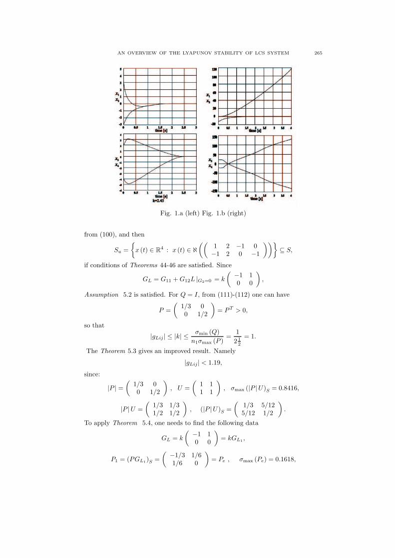
Fig. 1.a (left) Fig. 1.b (right)

from (100), and then

Su =

x (t) ∈ R4 : x (t) ∈ ℵ

((

1 2 −1 0−1 2 0 −1

))

⊆ S,

if conditions of Theorems 44-46 are satisfied. Since

GL = G11 +G12L |G2=0 = k

(

−1 10 0

)

,

Assumption 5.2 is satisfied. For Q = I, from (111)-(112) one can have

P =

(

1/3 00 1/2

)

= PT > 0,

so that

|gLij | ≤ |k| ≤σmin (Q)

n1σmax (P )=

1

2 12

= 1.

The Theorem 5.3 gives an improved result. Namely

|gLij| < 1.19,

since:

|P | =

(

1/3 00 1/2

)

, U =

(

1 11 1

)

, σmax (|P |U)S = 0.8416,

|P |U =

(

1/3 1/31/2 1/2

)

, (|P |U)S =

(

1/3 5/125/12 1/2

)

.

To apply Theorem 5.4, one needs to find the following data

GL = k

(

−1 10 0

)

= kGL1,

P1 = (PGL1)S =

(

−1/3 1/61/6 0

)

= Pe , σmax (Pe) = 0.1618,


k2 <1

σ2max (Pe)

⇒ |k| < 2.48.

Fig.1.a and Fig.1.b represent the system trajectories for possible values of uncertainparameter k. In the first case Fig.1.a, parameter k is chosen in such way that con-dition of Theorem 5.3 is satisfied, so the stability robustness of attraction propertyof origin is proved. It can be shown that quantitive measures obtained by Theorem

5.3 are less conservative than the other two [45]. The second case Fig.1.b, showsthat the required property is not achieved, since the choice of parameter k was notadequate.

7. Example 2

Consider a singular system given by

x1 (t) = (−1)x1 (t) +(

−1 −3)

x2 (t) +G1x (t) ,

0 =

(

−11

)

x1 (t) +

(

1 1−1 −1

)

x2 (t) .

Since det (cE −A) ≡ 0 for any c, this is an irregular singular system and solutionsare not unique. The following results can be obtained:

rank

(

−1 1 11 −1 −1

)

= rank

(

1 1−1 −1

)

= 1 ≤ 2

L =

(

a1− a

)

, a ∈ R , G2 ≡ 0,

From (110), one can get:

P = −1

a− 4, a < 4,

in order to have P = PT > 0. So

‖GL‖ ≤σmin (Q)

σmax (P )= − (a− 4)

and

Su =

x (t) ∈ R3 : x (t) ∈ ℵ

((

a −1 01− a 0 −1

))

, a < 4

⊆ S.

Two different values of parameter a could be chosen. The corresponding systemresponses can be analysed in the similar way, like in the example 1.

8. Conclusion

This review article deals with the stability of linear descriptor systems (LDS).Considering both regular and irregular continuous linear singular systems, signif-icant stability results concerning properties in the sense of Lyapunov have beenpresented. The relationship between them has been included in the study. Toassure asymptotical stability for linear continuous singular systems it is not onlyenough to have the eigenvalues of matrix pair (E, A) in the left half of the complexplane, but also to provide an impulse-free motion of the analyzed system.

Several different approaches in constructing the Lyapunov stability theory for aparticular class of linear continuous singular systems operating in free and forcedregimes have been presented. The same results have been used to test systemstabilty robustness. Some examples have been presented to show the applicabiltyof the derived results.


Acknowledgments

This work has been supported by The Ministry of Science and TechnologicalDevelopment of Serbia under Project ON 174 001.

References

[1] Bajic B.V., (1992) ’Lyapunov’s Direct Method in the Analysis of Singular Systems and Net-works’, Shades Technical Publication, Hillerest, Natal, RSA.

[2] Bajic B.V., Debeljkovic D., Gajic Z., Petrovic B., (1992) ’Weak Domain of Attraction and Ex-istence of Solutions Convergent to the Origin of the Phase Space of Singular Linear Systems’,University of Belgrade, ETF, Series: Automatic Control (1), pp.53-62.

[3] Bajic B.V, Milic M.M., (1986) ’Theorems on the Bounds of Solutions of Semi-State Models’,Int. J. Control, 43(3), pp.2183-2197.

[4] Bajic B.V., Milic M.M., (1987) ’Extended Stability of Motion of Semi-State Systems’, Int. J.of Control, 46(6), pp.2171-2181.

[5] Campbell S.L., (1980) ’Singular systems of differential equation I’, Pitman, London.[6] Campbell S.L., (1982) ’Singular Systems of Differential Equations II’, Pitman, Marshfield,

Mass.[7] Campbell S.L., Meyer C.D., Rose N.J., (1974) ’Application of Drazin Inverse to Linear System

of Differential Equations’, SIAM J. Appl. Math. Vol.31, pp.411-425.[8] Chen H.G., Kuang W.H., (1994) ’Improved quantitativemeasures of robustness for multivari-

able systems’, IEEE Trans. Autom. Contr., AC-39, No.4, pp.807-810.[9] Dai L., (1989) ’Singular Control Systems’, Lecture Notes in Control and Information Sciences,

Springer, Berlin, Vol.118.[10] Debeljkovic D.Lj., (2001) ’Stability of Linear Autonomous Singular Systems in the sense of

Lyapunov: An Overview’, NTP(YU), (in Serbian), Vol.LI, No.3, pp.70-79.[11] Debeljkovic D.Lj., (2002) ’Singular Control Systems’, Scientific Review, Series: Science and

Engineering, Vol.29-30, pp.139-162.[12] Debeljkovic D.Lj., (2004) ’Singular Control Systems’, Dynamics of Continuous, Discrete and

Impulsive Systems, Canada, Vol.11, Series A: Math. Analysis, No.5-6, pp.691-706.[13] Debeljkovic D.Lj., Bajic B.V., Gajic Z., Petrovic B., (1993) ’Boundedness and Existence of

Solutions of Regular and Irregular Singular Systems’, Publications of Faculty of ElectricalEng. Series: Automatic Control, Belgrade, YU, (1), pp.69-78.

[14] Debeljkovic D.Lj., Milinkovic S.A., Jovanovic M.B., (1996) ’Application of singular systemtheory in chemical engineering: Analysis of process dynamics’, Int. Congress of Chemical andProcess Eng., CHISA 96, Prague, Czech Rep., pp.25-30.

[15] Debeljkovic D.Lj., Milinkovic S.A., Jovanovic M.B., (2005) ’Continuous Singular ControlSystems’, GIP Kultura, Belgrade.

[16] Debeljkovic D.Lj., Milinkovic S.A., Jovanovic M.B., Jacic Lj.A., (2005) ’Discrete DescriptorControl Systems’, GIP Kultura, Belgrade.

[17] Djurovic V.K., Debeljkovic D.Lj., Milinkovic S.A., Jovanovic M.B., (1998) ’Further Results onLyapunov Stability Robustness Considerations for Linear Generalized State Space Systems’,AMSE, France, Vol.52, No.1-2, pp.54-64.

[18] Hu G., Sun J.T., (2003) ’Stability Analysis for Singular Systems With Time-Varying’, Journalof Tongji University, 31(4), pp.481-485.

[19] Isihara J.Y., Terra M.H., (2000) ’On the Lyapunov Theorem for Singular Systems’, IEEETrans. Automat. Control, AC-47, 11, pp.1926-1930.

[20] Lewis F.L., (1986) ’A Survey of Linear Singular Systems’, Circuits, Systems and SignalProcessing, 5(1), pp.3-36.

[21] Liu Y.Q., Li Y.Q., (1997) ’Stability of Solutions of a Class of Time-Varying Singular SystemsWith Delay’, Control and Decision, 12(3), pp.193-197.

[22] Luenberger D.G., (1977) ’Dynamic Equations in Descriptor Form’, IEEE Trans. Automat.Control, 22(3), pp.312-321.

[23] Masubuchi I., Kamitane Y., Ohara A., et al., (1997) ’Control for Descriptor Systems - AMatrix Inequalities Approach’, Automatica, 33(4), pp.669-673.

[24] Masubichi I., Shimemura E., (1997) ’An LMI Condition for Stability of Implicit Systems’,Proceedings of the 36th Conference on Decision and Control, San Diego, California, USA,pp.779-780.

[25] Men B., Zhang Q.L., Li X., Yang C., Chen Y., (2006) ’The Stabilty of Linear DescriptorSystems’, Intern. Journal of Inform. and System Science, Vol.2, No.3, pp.362-374.


[26] Muller P.C., (1997) ’Linear Mechanical Descriptor Systems: Identification, Analysis andDesign’, Preprints of IFAC, Conference on Control of Independent Systems, Belfort, France,pp.501-506.

[27] Owens H.D., Debeljkovic D.Lj., (1985) ’Consistency and Lyapunov Stability of Linear De-scriptor Systems: A Geometric Analysis”, IMA Journal of Mathematical Control and Infor-mation, 2(2), pp.139-151.

[28] Pandolfi L., (1980) ’Controlabillity and Stabilization for Linear System of Algebraic andDifferential Equations’, Jota 30(4), pp.601-620.

[29] Patel R.V., Toda M., (1980) ’Quantitative measures of robustness for multivariable systems’,Proc. Joint Control Conf., San Francisco, CA, USA, TP 8-A.

[30] Silva M.S., de Lima T.P., (2003) ’Looking for nonnegative solutions of a Leontief dynamicmodel’, Linear Algebra, 364, pp.281-316.

[31] Takaba K., (1998) ’Robust Control Descriptor System With Time-Varying Uncertainty’, Int.J. of Control, 71(4), pp.559-579.

[32] Tseng H.C., Kokotovic P.V., (1988) ’Optimal Control in Singularly Perturbed Systems: TheIntegral Manifold Approach’, IEEE Proc. on CDC, Austin, TX, USA, pp.1177-1181.

[33] Yang D.M., Zhang Q.L., Yao B., (2004) ’Descriptor Systems’, Science Publisher, Beijing.[34] Yedavalli R.K., (1985) ’Improved Measures of Stability Robustness for Linear State Space

Models’,IEEE Trans. Autom. Control,AC-30, No.6, pp.577-579.[35] Yedavalli R.K., Liang Z., (1986) ’Reduced Conservatism in Stability Robustness Bounds by

State Transformation’, IEEE Trans. Autom. Control, AC-31, No.9, pp.863-866.[36] Yue X.N., Zhang X.N., (1998) ’Analysis of Lyapunov Stability for Descriptor Systems’, Jour-

nal of Liaoning Educational Institute, 15(5), pp.42-44.[37] Zhang Q.L., (1997) ’Dispersal Control and Robust Control for Descriptor Systems’, North-

western Industrial University Publisher.[38] Zhang Q.L., Dai G.Z., Lam J., Zhang L.Q., (1998) ’The Asymptotic Stability and Stabiliza-

tion of Descriptor Systems’, Acta Automatica Sinica, 24(2), pp.208-312.[39] Zhang Q.L., Lam J., Zhang Q.L., (1999) ’Lyapunov and Riccati Equations of Discrete-Time

Descriptor Systems’, IEEE Trans. on Automatic Control, 44(11), pp.2134-2139.[40] Zhang Q.L., Lam J., Zhang L.Q., (1999) ’Generalized Lyapunov Equation for Analyzing the

Stability of Descriptor Systems’, Proc. of the 14th World Congress of IFAC, pp.19-24.[41] Zhang Q.L., Zhang L.Q., Nie Y.Y., (1999) ’Analysis and Synthesis of Robust Stability for

Descriptor Systems’, Control Theory and Applications, 16(4), pp.525-528.[42] Zhang J.H., Yu G.R., (2002) ’Analysis of Stability for Continuous Generalized Systems’,

Journal of Shenyang Institute of Aeronautical Engineering, Shenyang, 19(2), pp.67-69.[43] Zhang Q.L., Lam J., Zhang L.Q., (1999) ’New Lyapunov and Riccati Equations for Discrete

- Time Descriptor Systems’,Proc. of the 14th World Congress of IFAC, pp.7-12.[44] Zhang Q.L., Wang Q., Cong X., (2002) ’Investigation of Stability of Descriptor Systems’,

Journal of Northeastern University Natural Sciences, 23(7), pp.624-627.[45] Zhou K., Khargonekar P.P., (1987) ’Stability Robustness Bounds for Linear State-Space

Models with Structure Uncertainty’, IEEE Trans. Autom. Control, AC-32, No.7, pp.621-623.

1Department of Automatic Control, School of Mechanical Engineering, University of Belgrade,Belgrade, Serbia

E-mail : [email protected]

2Medical Physics Division, Thomas Jefferson University, Philadelphia, PA 19107, USAE-mail : [email protected]

lyapunov stability of linear continuous … · an overview of the lyapunov stability of lcs system...

Documents