m. bramanti - l. brandolini l estimates for …bramanti/pubblica/bramanti_brandolini_rendi... ·...
TRANSCRIPT

Rend. Sem. Mat. Univ. Pol. TorinoVol. 58, 4 (2000)
M. Bramanti - L. Brandolini
L P ESTIMATES FOR UNIFORMLY HYPOELLIPTIC
OPERATORS WITH DISCONTINUOUS COEFFICIENTS ON
HOMOGENEOUS GROUPS
Abstract. Let G be a homogeneous group and letX0, X1,. . . , Xq be left in-variant real vector fields onG, satisfying Hormander’s condition. Assume thatX1,. . . , Xq be homogeneous of degree one andX0 be homogeneous of degreetwo. We study operators of the kind:
L =q∑
i, j =1
ai j (x)Xi X j + a0(x)X0
whereai j (x) and a0(x) are real valued, bounded measurable functions belong-ing to the space “Vanishing Mean Oscillation”, defined with respect to the qua-sidistance naturally induced by the structure of homogeneous group. Moreover,the matrix{ai j (x)} is uniformly elliptic anda0(x) is bounded away from zero.
Under these assumptions we prove local estimates in the Sobolev spaceS2,p
(1 < p < ∞) defined by the vector fieldsXi , for solutions to the equationLu = fwith f ∈ Lp. From this fact we also deduce the local Holder continuity for solu-tions toLu = f , when f ∈ Lp with p large enough. Further (local) regularityresults, in terms of Sobolev or Holder spaces, are proved tohold when the coef-ficients and data are more regular. Finally, lower order terms (in the sense of thedegree of homogeneity) can be added to the operator mantaining the same results.
1. Introduction
A classical result of Agmon-Douglis-Nirenberg [1] states that, for a given uniformly ellipticoperator in nondivergence form with continuous coefficients,
Lu =∑
i, j
ai j (x) uxi x j
one has the followingL p-estimates for everyp ∈ (1,∞), on a bounded smooth domain� ofRn: ∥∥∥uxi x j
∥∥∥L p(�)
≤ c{‖Lu‖L p(�) + ‖u‖L p(�)
}.
While the above estimate is false in general if the coefficients are merelyL∞, a remarkableextension of the above result, due to Chiarenza-Frasca-Longo [6],[7], replaces the continuityassumption with the weaker conditionai j ∈ V M O, whereV M O is the Sarason’s space ofvanishing mean oscillation functions, a sort of uniform continuity in integral sense.
389

390 M. Bramanti - L. Brandolini
Roughly speaking, this extension relies on the classical theory of Calderon-Zygmu-nd op-erators, a theorem of Coifman-Rochberg-Weiss [8] (which wewill recall later in detail) aboutthe commutator of an operator of this type with aBM O function, and the knowledge of the fun-damental solution for constant coefficients elliptic operators onRn. All these ideas admit broadgeneralizations: the Calderon-Zygmund theory and the commutator theorem can be settled in thegeneral framework of spaces of homogeneous type, in the sense of Coifman-Weiss (see [9], [20]and [4]); however the knowledge of the fundamental solutionis a more subtle problem. Apartfrom the elliptic case, an explicit fundamental solution isalso known for constant coefficientsparabolic operators. This kernel is homogeneous with respect to the “parabolic dilations”, sothat the abstract Calderon-Zygmund theory can be applied to this situation to getL p-estimatesof the above kind for parabolic operators withV M O coefficients (see Bramanti-Cerutti [3]).
In recent years it has been noticed by Lanconelli-Polidoro [23] that an interesting classof ultraparabolic operators of Kolmogorov-Fokker-Plancktype, despite of its strong degener-acy, admits an explicit fundamental solution which turns out to be homogeneous with respectto suitable nonisotropic dilations, and invariant with respect to a group of (noncommutative)translations. These operators can be written as:
(1) Lu =q∑
i, j =1
ai j uxi x j +n∑
i, j =1
xi bi j ux j − ut
where(x, t) ∈ Rn+1,{bi j}
is a constant real matrix with a suitable upper triangular structure,while
{ai j}
is aq × q uniformly elliptic matrix, withq < n. The structure of space of homo-geneous type underlying the operator and the knowledge of a fundamental solution well shapedon this structure, suggest that an analogL p theory could be settled for operators of kind (1) withai j in V M O. This has been actually done by Bramanti-Cerutti-Manfredini [5] . (In this case,only local estimates are proved).
The class of operators (1) contains prototypes of Fokker-Planck operators describing brow-nian motions of a particle in a fluid, as well as Kolmogorov operators describing systems with 2ndegrees of freedom (see [23] ), and is still extensively studied (see for instance [22], [24], [25],[27] and references therein).
Whenai j = δi j , (1) exhibits an interesting example of “Hormander’s operator”, of the kind
Lu =q∑
i=1
X2i u + X0u
whereX0 =∑n
i, j =1 xi bi j ∂x j − ∂t , andXi = ∂xi for i = 1, 2, , . . . q. This introduces us to thepoint of view of hypoelliptic operators. Recall that a differential operatorP with C∞ coefficientsis said to be hypoelliptic in some open setU ⊆ RN if, whenever the equationPu = f is satisfiedin U by two distributionsu, f , then the following condition holds: ifV is an open subset ofUsuch thatf|V ∈ C∞(V), thenu|V ∈ C∞(V). We recall the well-known
THEOREM 1 (HORMANDER, [16]). Let X0, X1,. . . , Xq be real vector fields with coeffi-cients C∞(RN ). The operator
(2) P =q∑
i=1
X2i + X0
is hypoelliptic inRN if the Lie algebra generated at every point by the fields X0, X1,. . . , Xq isRN . We will call this property “Hormander’s condition”.

L p estimates for hypoelliptic operators 391
The operator (1) with constantai j ’s satisfies Hormander’s condition, by the structure as-sumption on the matrix
{bi j}, and is therefore hypoelliptic.
In ’75, Folland [11] proved that any Hormander’s operator like (2) which is left invariantwith respect to a group of translations, and homogeneous of degree 2 with respect to a familyof (nonisotropic) dilations, which are group automorphisms, has a homogeneous left invariantfundamental solution. This allows to apply the abstract theory of singular integrals in spaces ofhomogeneous type, to get localL p estimates of the kind
(3)∥∥Xi X j u
∥∥Lp(�′) ≤ c
{‖Lu‖Lp(�) + ‖u‖Lp(�)
}(i, j = 1, . . . , q)
for any p ∈ (1,∞) , �′ ⊂⊂ �.
Motivated by the results obtained by [3], [5], the aim of thispaper is to extend the abovetechniques and results to the homogeneous setting considered by Folland, where good propertiesof the fundamental solution allow to obtain in a natural way theL p estimates, using the availablereal variable machinery.
More precisely, we study operators of the kind:
L =q∑
i, j =1
ai j (x)Xi X j + a0(x)X0
whereX0, X1,. . . , Xq form a system ofC∞ real vector fields defined inRN (N ≥ q + 1), satis-fying Hormander’s condition. We also assume thatX0, X1,. . . , Xq are left invariant with respectto a “translation” which makesRN a Lie group, and homogeneous with respect to a family of“dilations” which are group automorphisms. More precisely, X1,. . . , Xq are homogeneous ofdegree one andX0 is homogeneous of degree two. The coefficientsai j (x), a0(x) are real valuedbounded measurable functions, satisfying very weak regularity conditions (they belong to theclassV M O, “Vanishing Mean Oscillation”, defined with respect to the homogeneous distance;in particular, they can be discontinuous); moreover, the matrix {ai j (x)} is uniformly elliptic andnot necessarily symmetric; the functiona0(x) is bounded away from zero.
Under these assumptions (see §2 for precise statements) we prove that the localLp estimates(3) hold for p ∈ (1, ∞), every bounded domain�, any�′ ⊂⊂ �, and anyu for which the righthand side of (3) makes sense (see Theorem 3 for a precise statement). From this fact we alsodeduce the local Holder continuity for solutions to the equationLu = f , when f ∈ Lp(�) withp large enough (see Theorem 4).
To get (3) we will first prove the following estimate:
(4)∥∥Xi X j u
∥∥p ≤ c‖Lu‖p (i, j = 1, . . . , q, 1 < p < ∞),
for every test functionu supported in a ball with sufficiently small radius (see Theorem 2). It isin this estimate that theV M O regularity of the coefficients plays a crucial role.
Further (local) regularity results for solutions to the equationLu = f , in terms of Sobolev orHolder spaces, are proved to hold when the coefficients and data are more regular (see Theorems5, 6). Finally, lower order terms (in a suitable sense) can beadded to the operator maintainingthe same results (see Theorem 7).
Since the operatorL has, in general, nonsmooth coefficients, the above definition of hypoel-lipticity makes no sense forL. However we will show (Theorem 8) that if the coefficientsai j (x)
are smooth, thenL is actually hypoelliptic. Moreover, for every fixedx0 ∈ RN , the frozen

392 M. Bramanti - L. Brandolini
operator
(5) L0 =q∑
i, j =1
ai j (x0)Xi X j + a0(x0)X0
is always hypoelliptic and, by the results of Folland [11] (see Theorem 9 below), has a homoge-neous fundamental solution, which we will prove to satisfy some uniform bounds, with respectto x0 (Theorem 12). This perhaps justifies the (improper) name of “uniformly hypoelliptic oper-ators” forL, which appears in the title.
We point out that the results in this paper contain as particular cases the local estimatesproved in [6], [3] and [5]. On the other side, globalL p estimates on a domain are not availablefor hypoelliptic operators, even in simple model cases.
A natural issue is to discuss the necessity of our homogeneity assumptions. In a famouspaper, Rothschild-Stein [28] introduced a powerful technique of “lifting and approximation”,which allows to study a general Hormander’s operator by means of operators of the kind studiedby Folland. As a consequence, they obtained estimates like (3) in this more general setting.
In a forthcoming paper [2], we shall use their techniques, combined with our results, toattack the general case where the homogeneous structure underlying the Hormander’s vectorfields is lacking.
Outline of the paper. §§2.1, 2.2, 2.5 contain basic definitions and known results.In §2.3we state our main results (Theorems 2 to 7 ). In §2.4 we illustrate the relations between ourclass of operators and the operators of Hormander type, comparing our results with those ofRothschild-Stein [28].
In §3 we prove Theorem 2 (that is (4)). The basic tool is the fundamental solution of thefrozen operator (5), whose existence is assured by [11] (see§3.1. The line of the proof consistsof three steps:
(i ) we write a representation formula for the second order derivatives of a test function interms of singular integrals and commutators of singular integrals involving derivatives of thefundamental solution (see §3.2);
(i i ) we expand the singular kernel in series of spherical harmonics, to get singular integralsof convolution-type, with respect to our group structure (see §3.3); this step is necessary due tothe presence of the variable coefficientsai j (x) in the differential operator;
(i i i ) we getLp-bounds for the singular integrals of convolution-type andtheir commutators,applying general results for singular integrals on spaces of homogeneous type (see §3.4).
This line is the same followed in [5], which in turn was inspired by [6], [7]. While the com-mutator estimate needed in [6], [7] to achieve point (i i i ) is that proved by Coifman-Rochberg-Weiss in [8], the suitable extension of this theorem to spaces of homogeneous type has beenproved by Bramanti-Cerutti in [4].
The basic difficulty to overcome in the present situation, due to the class of differential op-erators we are considering, is that an explicit form for the fundamental solution of the frozenoperatorL0 in (5) is in general unknown. Therefore we have to prove in an indirect way uni-form bounds with respect tox0 for the derivatives of the fundamental solutions correspondingto L0 (Theorem 12). This will be a key point, in order to reduce the proof of (3) to that ofLp
boundedness for singular integrals of convolution type. Wewish to stress that, although severaldeep results have been proved about sharp bounds for the fundamental solution of a hypoellipticoperator (see [26], [29], [19]), these bounds are proved fora fixed operator, and the dependenceof the constants on the vector fields is not apparent: therefore, these results cannot be applied in

L p estimates for hypoelliptic operators 393
order to get uniform bounds for families of operators. On theother side, a useful point of viewon this problem has been developed by Rothschild-Stein [28], and we will adapt this approach toour situation. To make more readable the exposition, the proof of this uniform bound (Theorem12) is postponed to §4.
To prove local estimates for solutions to the equationLu = f , starting from our basic es-timate (4), we need some properties of the Sobolev spaces generated by the vector fieldsXi ,which we investigate in §5: interpolation inequalities, approximation results, embedding theo-rems. Some of these results appear to be new and can be of independent interest, because theyregard spaces of functions not necessarily vanishing at theboundary, whereas in [11] or [28], forinstance, only Sobolev spaces of functions defined on the whole space are considered.
In §6 we apply all the previous theory to local estimates for solutions toLu = f . Firstwe prove (3) and the local Holder continuity of solutions (see Theorems 4, 5). Then we provesome regularity results, in the sense of Sobolev or Holder spaces (see Theorems 5, 6), whenthe coefficients are more regular, as well as the generalization of all the previous estimates tothe operator with lower order terms (Theorem 7). Observe that, since the vector fields do notcommute, estimates on higher order derivatives are not a straightforward consequence of thebasic estimate (3). Instead, we shall prove suitable representation formulas for higher orderderivatives and then apply again the machinery of §3.
2. Definitions, assumptions and main results
2.1. Homogeneous groups and Lie algebras
Following Stein (see [31], pp. 618-622) we call homogeneousgroup the spaceRN equippedwith a Lie group structure, together with a family of dilations that are group automorphisms.Explicitly, assume that we are given a pair of mappings:
[(x, y) 7→ x ◦ y] : RN × R
N → RN and
[x 7→ x−1
]: R
N → RN
that are smooth and so thatRN , together with these mappings, forms a group, for which theidentity is the origin. Next, suppose that we are given anN-tuple of strictly positive exponentsω1 ≤ ω2 ≤ . . . ≤ ωN , so that the dilations
(6) D(λ) : (x1, . . . ,xN ) 7→(λω1x1, . . . , λωN xN
)
are group automorphisms, for allλ > 0. We will denote byG the spaceRN with this structureof homogeneous group, and we will writec(G) for a constant depending on the numbersN,ω1,. . . , ωN and the group law◦.
We can define inRN a homogeneous norm‖·‖ as follows. For anyx ∈ RN , x 6= 0, set
‖x‖ = ρ ⇔∣∣∣∣D(
1
ρ)x
∣∣∣∣ = 1,
where|·| denotes the Euclidean norm; also, let‖0‖ = 0. Then:
(i) ‖D(λ)x‖ = λ ‖x‖ for everyx ∈ RN , λ > 0;
(ii) the set{x ∈ RN : ‖x‖ = 1} coincides with the Euclidean unit sphere∑
N ;
(iii) the functionx 7→ ‖x‖ is smooth outside the origin;
(iv) there existsc(G) ≥ 1 such that for everyx, y ∈ RN
(7) ‖x ◦ y‖ ≤ c(‖x‖ + ‖y‖) and∥∥∥x−1
∥∥∥ ≤ c‖x‖ ;

394 M. Bramanti - L. Brandolini
(8)1
c|y| ≤ ‖y‖ ≤ c |y|1/ω if ‖y‖ ≤ 1, withω = max(ω1, . . . , ωN ) .
The above definition of norm is taken from [12]. This norm is equivalent to that defined in[31], but in addition satisfies (ii), a property we shall use in §3.3. The properties (i),(ii) and (iii)are immediate while (7) is proved in [31], p. 620 and (8) is Lemma 1.3 of [11].
In view of the above properties, it is natural to define the “quasidistance”d:
d(x, y) =∥∥∥y−1 ◦ x
∥∥∥ .
Ford the following hold:
(9) d(x, y) ≥ 0 and d(x, y) = 0 if and only if x = y;
(10)1
cd(y,x) ≤ d(x, y) ≤ c d(y,x);
(11) d(x, y) ≤ c(d(x, z) + d(z, y)
)
for every x, y, z ∈ RN and some positive constantc(G) ≥ 1. We also define the balls withrespect to d as
B(x, r ) ≡ Br (x) ≡{
y ∈ RN : d(x, y) < r
}.
Note thatB(0, r ) = D(r )B(0,1). It can be proved (see [31], p. 619) that the Lebesgue measurein RN is the Haar measure ofG. Therefore
(12) |B(x, r )| = |B(0,1)| r Q,
for everyx ∈ RN andr > 0, whereQ = ω1 + . . . + ωN , with ωi as in (6). We will callQ thehomogeneous dimension ofRN . By (12) the Lebesgue measuredx is a doubling measure withrespect tod, that is
|B(x, 2r )| ≤ c · |B(x, r )| for everyx ∈ RN andr > 0
and therefore (RN ,dx, d) is a space of homogenous type in the sense of Coifman-Weiss (see[9]). To be more precise, the definition of space of homogenous type in [9] requiresd to besymmetric, and not only to satisfy (10). However, the results about spaces of homogeneous typethat we will use still hold under these more general assumptions. (See Theorem 16).
We say that a differential operatorY onRN is homogeneous of degreeβ > 0 if
Y(
f((D(λ)x
))= λβ (Y f)(D(λ)x)
for every test functionf , λ > 0, x ∈ RN . Also, we say that a functionf is homogeneous ofdegreeα ∈ R if
f((D(λ)x)
)= λα f (x) for everyλ > 0, x ∈ R
N .
Clearly, ifY is a differential operator homogeneous of degreeβ and f is a homogeneous functionof degreeα, thenY f is homogeneous of degreeα − β.
Let us consider now the Lie algebra` associated to the groupG (that is, the Lie algebra ofleft-invariant vector fields). We can fix a basisX1,. . .,XN in ` choosingXi as the left invariant

L p estimates for hypoelliptic operators 395
vector field which agrees with∂∂xi
at the origin. It turns out thatXi is homogeneous of degreeωi (see [11], p. 164). Then, we can extend the dilationsD(λ) to ` setting
D(λ) Xi = λωi Xi .
D(λ) turns out to be a Lie algebra automorphism, i.e.,
D(λ) [X, Y] = [D(λ)X, D(λ)Y] .
In this sense, is said to be a homogeneous Lie algebra; as a consequence,` is nilpotent (see[31], p. 621-2).
Recall that a Lie algebrais said to be graded if it admits a vector space decompositionas
` =r⊕
i=1
Vi with[Vi ,Vj
]⊆ Vi+ j for i + j ≤ r ,
[Vi ,Vj
]= {0} otherwise.
In this paper, will always be graded and it will be possible to chooseVi as the set of vectorfields homogeneous of degreei .
Also, a homogeneous Lie algebra is called stratified if thereexists vector spacesV1, . . . , Vssuch that
` =s⊕
i=1
Vi with[V1, Vi
]= Vi+1 for 1 ≤ i < s and
[V1, Vs
]= {0}.
This implies that the Lie algebra generated byV1 is the whole . Clearly, if ` is stratifiedthen` is also graded.
Throughout this paper, we will deal with two different situations:
Case A.There existq vector fields (q ≤ N) X1,. . . , Xq, homogeneous of degree 1 such thatthe Lie algebra generated by them is the whole`. Therefore is stratified andV1 is spanned byX1,. . . , Xq. In this case the “natural” operator to be considered is
(13) L =q∑
i=1
X2i ,
which is hypoelliptic, left invariant and homogeneous of degree two.
EXAMPLE 1. The simplest (nonabelian) example of Case A is the Kohn-Laplacian on the
Heisenberg groupG =(R3, ◦, D(λ)
)where:
(x1, y1, t1) ◦ (x2, y2, t2) =
= (x1 + x2, y1 + y2, t1 + t2 + 2(x2y1 − x1y2))
andD(λ) (x, y, t) =
(λx, λy, λ2t
).
X = ∂
∂x+ 2y
∂
∂t; Y = ∂
∂y− 2x
∂
∂t; [X, Y] = −4
∂
∂t;
` = V1 ⊕ V2 with V1 = 〈X, Y〉.

396 M. Bramanti - L. Brandolini
The fieldsX,Y are homogeneous of degree 1, and the operator
L = X2 + Y2
is hypoelliptic and homogeneous of degree two. Here the homogeneous dimension ofG isQ = 4.
Case B.There existq + 1 vector fields (q + 1 ≤ N) X0, X1,. . . , Xq, such that the Lie al-gebra generated by them is the whole`, X1,. . . , Xq are homogeneous of degree 1 andX0 ishomogeneous of degree 2. In this case the “natural” operatorto be considered is
(14) L =q∑
i=1
X2i + X0.
Under these assumptions` may or may not be stratified (see examples below).
EXAMPLE 2. (Kolmogorov-type operators, studied in [23]).
ConsiderG =(R3, ◦, D(λ)
)with:
(x1, y1, t1) ◦ (x2, y2, t2) = (x1 + x2, y1 + y2 − x1t2, t1 + t2)
andD(λ) (x, y, t) =
(λx, λ3y, λ2t
).
X1 =∂
∂x; X0 =
∂
∂t− x
∂
∂y;[X0, X1
]=
∂
∂y;
(15) ` = V1 ⊕ V2 with V1 = 〈X1, X0〉, V2 = 〈 ∂
∂y〉
therefore is stratified; the fieldsX1, X0 are homogeneous of degree 1 and 2, respectively, andthe operator
L = X21 + X0
is hypoelliptic and homogeneous of degree two. Note that in this case the stratification (15) of`
is different from the natural decomposition of` as a graded algebra:
` = V1 ⊕ V2 ⊕ V3 with V1 = 〈X1〉, V2 = 〈X0〉, V3 = 〈 ∂
∂y〉.
This is the simplest (nonabelian) example of Case B; note that Q = 6. If, keeping the samegroup law◦, we changed the definition ofD(λ) setting
D(λ) (x, y, t) =(λx, λ2y, λt
),
then the fieldsX0, X1 would be homogeneous of degree one, and we should consider the operator
L = X21 + X2
0,
as in Case A.

L p estimates for hypoelliptic operators 397
EXAMPLE 3. This is an example of the non-stratified case.
ConsiderG =(R5, ◦, D(λ)
)with:
(x1, y1, z1, w1,t1) ◦ (x2, y2, z2, w2, t2) =
= (x1 + x2, y1 + y2, z1 + z2, w1 + w2 + x1y2,
t1 + t2 − x1x2y1 − x1x2y2 −1
2x22 y1 + x1w2 + x1z2)
andD(λ) (x, y, z, w, t) =
(λx, λy, λ2z, λ2w, λ3t
).
The natural base for consists of:
X =∂
∂x− xy
∂
∂t; Y =
∂
∂y+ x
∂
∂w; Z =
∂
∂z+ x
∂
∂t;
W =∂
∂w+ x
∂
∂t; T =
∂
∂t.
We can see that is graded setting
` = V1 ⊕ V2 ⊕ V3 with V1 = 〈X, Y〉, V2 = 〈Z, W〉, V3 = 〈T〉.
The nontrivial commutation relations are:
[X,Y] = W; [X, Z] = T ; [X, W] = T.
Therefore, if we setV1 = 〈X, Y, Z〉, we see that the Lie algebra generated byV1 is `; moreoverV2 =
[V1, V1
]= 〈W, T〉 and V3 =
[V1, V2
]= 〈T〉, so that` is not stratified. Noting that
X, Y, Z are homogeneous of degrees 1, 1, 2 respectively, we have that the operator
L = X2 + Y2 + Z
is hypoelliptic and homogeneous of degree two.
2.2. Function spaces
Before going on, we need to introduce some notation and function spaces. First of all, ifX0,X1,. . . , Xq are the vector fields appearing in (13)-(14), define, forp ∈ [1,∞]
‖Du‖p ≡q∑
i=1
‖Xi u‖p ;
∥∥∥D2u∥∥∥
p≡
q∑
i, j =1
∥∥Xi X j u∥∥
p + ‖X0u‖p .
More in general, set ∥∥∥Dku∥∥∥
p≡∑∥∥X j1 . . . X jl u
∥∥p
where the sum is taken over all monomialsX j1 . . . X jl homogeneous of degreek. (Note thatX0has weight two while the remaining fields have weight one. Obviously, in Case A the fieldX0

398 M. Bramanti - L. Brandolini
does not appear in the definition of the above norms). Let� be a domain inRN , p ∈ [1,∞] andk be a nonnegative integer. The spaceSk,p (�) consists of allLp (�) functions such that
‖u‖Sk,p(�) =k∑
h=0
∥∥∥Dhu∥∥∥Lp(�)
is finite. We shall also denote bySk,p0 (�) the closure ofC∞
0 (�) in Sk,p (�).
Since we will often consider the casek = 2, we will briefly write Sp (�) for S2,p (�) and
Sp0 (�) for S2,p
0 (�).
Note that the fieldsXi , and therefore the definition of the above norms, are completelydetermined by the structure ofG.
We define the Holder spaces3k,α(�), for α ∈ (0, 1), k nonnegative integer, setting
|u|3α(�) = supx 6=y
x,y∈�
|u(x) − u(y)|d(x, y)α
and
‖u‖3k,α (�) =∣∣∣Dku
∣∣∣3α(�)
+k−1∑
j =0
∥∥∥D j u∥∥∥L∞(�)
.
In §4, we will also use the fractional (but isotropic) Sobolev spacesH t,2(RN
), defined in the
usual way, setting, fort ∈ R,
‖u‖2H t,2 =
∫
RN|u(ξ)|2
(1 + |ξ |2
)tdξ ,
whereu(ξ) denotes the Fourier transform ofu.
The structure of space of homogenous type allows us to define the space of Bounded MeanOscillation functions (BM O, see [18]) and the space of Vanishing Mean Oscillation functions(V M O, see [30]). If f is a locally integrable function, set
(16) η f (r ) = supρ<r
1∣∣Bρ
∣∣∫
Bρ
∣∣∣ f (x) − fBρ
∣∣∣ dx for everyr > 0,
whereBρ is any ball of radiusρ and fBρis the average off over Bρ .
We say thatf ∈ BM O if ‖ f ‖∗ ≡ supr η f (r ) < ∞.
We say thatf ∈ V M O if f ∈ BM O andη f (r ) → 0 for r → 0.
We can also define the spacesBM O(�) andV M O (�) for a domain� ⊂ RN , just replac-ing Bρ with Bρ ∩ � in (16).
2.3. Assumptions and main results
We now state precisely our assumptions, keeping all the notation of §§2.1, 2.2.
Let G be a homogeneous group of homogeneous dimensionQ ≥ 3 and` its Lie algebra; let{Xi } (i = 1, 2, . . . , N) be the basis of constructed as in §2.1, and assume that the conditions of

L p estimates for hypoelliptic operators 399
Case A or Case B hold. Accordingly, we will study the following classes of operators, modeledon the translation invariant prototypes (13), (14):
L =q∑
i, j =1
ai j (x)Xi X j
or
(17) L =q∑
i, j =1
ai j (x)Xi X j + a0(x)X0
whereai j anda0 are real valued bounded measurable functions and the matrix{ai j (x)
}satisfies a uniform ellipticity condition:
(18) µ |ξ |2 ≤q∑
i, j =1
ai j (x) ξi ξ j ≤ µ−1 |ξ |2 for everyξ ∈ Rq, a.e.x,
for some positive constantµ. Analogously,
(19) µ ≤ a0(x) ≤ µ−1.
Moreover, we will assumea0, ai j ∈ V M O.
Then:
THEOREM2. Under the above assumptions, for every p∈ (1,∞) there exist c= c(p, µ, G)
and r = r (p, µ, η, G) such that if u∈ C∞0
(RN
)and sprt u⊆ Br (Br any ball of radius r)
then ∥∥∥D2u∥∥∥
p≤ c‖Lu‖p
whereη denotes dependence on the “V M O moduli” of the coefficients a0, ai j .
THEOREM3 (LOCAL ESTIMATES FOR SOLUTIONS TO THE EQUATION
Lu = f IN A DOMAIN ). Under the above assumptions, let� be a bounded domain ofRN and�′ ⊂⊂ �. If u ∈ Sp (�), then
‖u‖Sp(�′) ≤ c{‖Lu‖Lp(�) + ‖u‖Lp(�)
}
where c= c(p, G, µ, η, �,�′).
THEOREM4 (LOCAL HOLDER CONTINUITY FOR SOLUTIONS TO THE
EQUATION Lu = f IN A DOMAIN ). Under the assumptions of Theorem 3, if u∈ Sp (�) forsome p∈ (1, ∞) andLu ∈ Ls(�) for some s> Q/2, then
‖u‖3α(�′) ≤ c{‖Lu‖Lr (�) + ‖u‖Lp(�)
}
for r = max(p, s), α = α(Q, p, s) ∈ (0, 1), c = c(G, µ, p, s, �,�′).

400 M. Bramanti - L. Brandolini
THEOREM5 (REGULARITY OF THE SOLUTION IN TERMS OFSOBOLEV SPACES). Underthe assumptions of Theorem 3, if a0, ai j ∈ Sk,∞(�), u ∈ Sp (�) andLu ∈ Sk,p (�) for somepositive integer k (k even, in Case B),1 < p < ∞, then
‖u‖Sk+2,p(�′) ≤ c1
{‖Lu‖Sk,p(�) + c2 ‖u‖Lp(�)
}
where c1 = c1(p, G, µ,η,�, �′) and c2 depends on the Sk,∞(�) norms of the coefficients.
THEOREM6 (REGULARITY OF THE SOLUTION IN TERMS OFHOLDER
SPACES). Under the assumption of Theorem 3, if a0, ai j ∈ Sk,∞(�), u ∈ Sp (�) andLu ∈Sk,s (�) for some positive integer k (k even, in Case B),1 < p < ∞, s > Q/2, then
‖u‖3k,α (�′) ≤ c1
{‖Lu‖Sk,r (�) + c2 ‖u‖Lp(�)
}
where r =max(p, s), α = α(Q, p, s) ∈ (0, 1), c1 = c1(p, s, k, G, µ,η,�,�′) and c2 dependson the Sk,∞(�) norms of the coefficients.
THEOREM 7 (OPERATORS WITH LOWER ORDER TERMS). Consider an operator with“lower order terms” (in the sense of the degree of homogeneity), of the following kind:
L ≡( q∑
i, j =1
ai j (x)Xi X j + a0(x)X0
)+( q∑
i=1
ci (x)Xi + c0 (x)
)≡
≡ L2 + L1.
i) If ci ∈ L∞ (�) for i = 0, 1, . . . , q, then:
if the assumptions of Theorem 3 hold forL2, then the conclusions of Theorem 3 hold forL;
if the assumptions of Theorem 4 hold forL2, then the conclusions of Theorem 4 hold forL.
ii) If c i ∈ Sk,∞(�) for some positive integer k, i= 0, 1, . . . , q, then:
if the assumptions of Theorem 5 hold forL2, then the conclusions of Theorem 5 hold forL;
if the assumptions of Theorem 6 hold forL2, then the conclusions of Theorem 6 hold forL.
REMARK 1. Since all our results are local, it is unnatural to assume that the coefficientsa0,ai j be defined on the wholeRN . Actually, it can be proved that any functionf ∈ V M O(�),
with � bounded Lipschitz domain, can be extended to a functionf defined inRN with V M Omodulus controlled by that off . (For more details see [3]). Therefore, all the results of Theorems2, 7 still hold if the coefficients belong toV M O(�), but it is enough to prove them fora0,ai j ∈ V M O.
2.4. Relations with operators of Hormander type
Here we want to point out the relationship between our class of operators and operators ofHormander type (2).
THEOREM8. Under the assumptions of §2.3:
(i) if the coefficients ai j (x) are Lipschitz continuous (in the usual sense), then the operatorL can be rewritten in the form
L =q∑
i=1
Y2i + Y0

L p estimates for hypoelliptic operators 401
where the vector fields Yi (i = 1, . . . , q) have Lipschitz coefficients and Y0 has bounded mea-surable coefficients;
(ii ) if the coefficients ai j (x) are smooth (C∞), thenL is hypoelliptic;
(iii ) if the coefficients ai j are constant, thenL is left invariant and homogeneous of degree
two; moreover, the transposeLT ofL is hypoelliptic, too.
Proof. Let us split the matrixai j (x) in its symmetric and skew-symmetric parts:
ai j (x) = 1
2
(ai j (x) + a j i (x)
)+ 1
2
(ai j (x) − a j i (x)
)≡ bi j (x) + bi j (x).
If the matrix A ={ai j (x)
}satisfies condition (18), the same holds forB =
{bi j (x)
}. Therefore
we can writeB = M MT whereM = {mi j (x)} is an invertible, triangular matrix, whose entriesareC∞ functions of the entries ofB.
To see this, we can use the “method of completion of squares” (seee.g. [17], p. 180),writing
q∑
i, j =1
bi j ξi ξ j = η21 +
q∑
i, j =2
b∗i j ηi η j
with
η1 =
√b11ξ1 +
q∑
j =2
b1 j√b11
ξ j
; ηi = ξi for i ≥ 2;
b∗i i = bi i −
b21i
b11; b∗
i j = bi j for i, j = 2, . . . , q, i 6= j .
Since(η1, . . . , ηq
)are a linear invertible function of
(ξ1, . . . , ξq
), and the quadratic form∑q
i, j =1 bi j ξi ξ j is positive (onRq), also the quadratic form∑q
i, j =2 b∗i j ηi η j is positive (on
Rq−1), and we can iterate the same procedure. Note thatη1 =∑q
k=1 m1kξk with m1k smoothfunctions of thebi j ’s; moreover,b∗
i j are smooth functions of thebi j ’s. Therefore iteration of thisprocedure allows us to write
q∑
i, j =1
bi j ξi ξ j =q∑
k=1
λ2k with:
λk =q∑
h=k
mkhξh and mkh are smooth functions of thebi j ’s.
This means thatbi j =∑
k≥i, j mki mkj with mkh smooth functions of thebi j ’s.
Therefore we can write:
L =q∑
i, j =1
q∑
k=1
mik (x) m j k(x)Xi X j +∑
i< j
bi j (x)[Xi ,X j
]+ a0(x)X0
where the functionsmik (x) have the same regularity of theai j (x)’s. (To simplify the notation,from now on we forget the fact thatmik = 0 if k < i ). If the ai j (x)’s are Lipschitz continuous,the above equation can be rewritten as
(20) L =q∑
k=1
Y2k + Y0

402 M. Bramanti - L. Brandolini
with
Yk =q∑
i=1
mik (x)Xi and
Y0 =∑
i< j
bi j (x)[Xi ,X j
]+ a0(x)X0 −
q∑
i, j =1
q∑
k=1
mik (x) ·(
Xi m j k (x)
)X j ,
which proves (i). If the coefficientsai j (x) areC∞, theYi ’s areC∞ vector fields and satisfyHormander’s condition, because every linear combinationof the Xi (i = 0, 1, . . . , q) can berewritten as a linear combination of theYi and their commutators of length 2. Therefore, byTheorem 1,L is hypoelliptic, that is (ii). Finally, if the coefficientsai j are constant, then (20)holds with
Yk =q∑
i=1
mik Xi and Y0 =∑
i< j
bi j[Xi ,X j
]+ a0 X0,
which means thatL is left invariant and homogeneous of degree two. Moreover, since the fieldsXi are translation invariant, the transposeXT
i of Xi equals−Xi and as a consequenceLT ishypoelliptic as well. This proves(iii ).
REMARK 2. By the above Theorem, ifai j ∈ C∞, our class of operators is contained in thatstudied by Rothschild-Stein [28], so in this case our results follow from [28], without assumingthe existence of a structure of homogeneous group. If the coefficients are less regular, but at leastLipschitz continuous, our operators can be written as “operators of Hormander type”; however,in this case we cannot check Hormander’s condition for the fieldsYi and therefore our estimatesdo not follow from known results about hypoelliptic operators. Finally, if the coefficients aremerelyV M O, we cannot even writeL in the form (20).
2.5. More properties of homogeneous groups
We recall some known results which will be useful later. First of all, we define the convolutionof two functions inG as
( f ∗ g)(x) =∫
RNf (x ◦ y−1) g(y) dy =
∫
RNg(y−1 ◦ x) f (y) dy,
for every couple of functions for which the above integrals make sense. From this definition weread that ifP is any left invariant differential operator,
P( f ∗ g) = f ∗ Pg
(provided the integrals converge). Note that, ifG is not abelian, we cannot writef ∗Pg = P f ∗g.Instead, ifX andXR are, respectively, a left invariant and right invariant vector field which agreeat the origin, the following hold (see [31], p. 607)
(21) (X f ) ∗ g = f ∗(
XRg)
; XR ( f ∗ g) =(
XR f)
∗ g.
In view of the above identities, we will sometimes use the right invariant vector fieldsXRi which
agree with∂/∂xi (and therefore withXi ) at the origin (i = 1, . . . , N), and we need some prop-

L p estimates for hypoelliptic operators 403
erties linkingXi to XRi . It can be proved that
Xi = ∂
∂xi+
N∑
k=i+1
qki (x)
∂
∂xk
XRi =
∂
∂xi+
N∑
k=i+1
qki (x)
∂
∂xk
whereqki (x), qk
i (x) are polynomials, homogeneous of degreeωk−ωi (theωi ’s are the exponentsappearing in (6)). From the above equations we find that
Xi =N∑
k=i
cki (x) XR
k
wherecki (x) are polynomials, homogeneous of degreeωk−ωi . In particular, sinceωk−ωi < ωk,
cki (x) does not depend onxh for h ≥ k and therefore commutes withXR
k , that is
(22) Xi u =N∑
k=i
XRk
(cki (x) u
)(i = 1, . . . , N)
for every test functionu. This representation ofXi in terms ofXRi will be useful in §6.
THEOREM 9. (See Theorem 2.1 and Corollary 2.8 in[11]). Let L be a left invariantdifferential operator homogeneous of degree two on G, such thatL andLT are both hypoelliptic.Moreover, assume Q≥ 3. Then there is a unique fundamental solution0 such that:
(a) 0 ∈ C∞(RN \ {0}
);
(b) 0 is homogeneous of degree(2 − Q);
(c) for every distributionτ ,
L (τ ∗ 0) = (Lτ) ∗ 0 = τ.
THEOREM 10. (See Proposition 8.5 in[13]), Proposition 1.8 in[11])). Let Kh be a kernelwhich isC∞
(RN \ {0}
)and homogeneous of degree(h − Q), for some integer h with0 < h < Q; let
Th be the operatorTh f = f ∗ Kh
and let Ph be a left invariant differential operator homogeneous of degree h.
Then:PhTh f = P.V.
(f ∗ Ph Kh
)+ α f
for some constantα depending on Ph and Kh;
the function Ph Kh is C∞(RN \ {0}
), homogeneous of degree−Q and satisfies the van-
ishing property: ∫
r<‖x‖<RPhKh (x) dx = 0 for 0 < r < R < ∞;

404 M. Bramanti - L. Brandolini
the singular integral operator
f 7→ P.V.(
f ∗ Ph Kh
)
is continuous onLp for 1 < p < ∞.
To handle the convolution of several kernels, we will need also the following
LEMMA 1. Let K1 (·, ·), K2(·, ·) be two kernels satisfying the following:
(i) for every x∈ RN Ki (x, ·) ∈ C∞(RN \ {0}) (i = 1, 2);
(ii) for every x∈ RN Ki (x, ·) is homogeneous of degreeαi , with−Q < αi < 0, α1+α2 <
−Q;
(iii ) for every multiindexβ,
supx∈RN
sup‖y‖=1
∣∣∣∣∣
(∂
∂y
)β
Ki (x, y)
∣∣∣∣∣ ≤ cβ .
Then, for every test function f and any x0, y0 ∈ RN ,
( f ∗ K1(x0, ·)) ∗ K2(y0, ·) = f ∗ (K1(x0, ·) ∗ K2(y0, ·)) .
Moreover, setting K(x0, y0,·) = K1(x0, ·) ∗ K2(y0, ·), we have the following:
(iv) for every(x0, y0) ∈ R2N , K(x0, y0,·) ∈ C∞(RN \ {0});(v) for every(x0, y0) ∈ R2N , K(x0, y0,·) is homogeneous of degreeα1 + α2 + Q;
(vi) for every multiindexβ,
(23) sup(x,y)∈R2N
sup‖z‖=1
∣∣∣∣∣
(∂
∂z
)β
K (x, y, z)
∣∣∣∣∣ ≤ cβ .
The above Lemma has been essentially proved by Folland (see Proposition 1.13 in [11]),apart from the uniform bound onK , which follows reading carefully the proof.
3. Proof of Theorem 2
All the proofs in this section will be written for the Case B. The results in Case A (which iseasier) simply follow dropping the termX0.
3.1. Fundamental solutions
For anyx0 ∈ RN , let us “freeze” atx0 the coefficientsai j (x), a0(x) of the operator (17), andconsider
(24) L0 =q∑
i, j =1
ai j (x0)Xi X j + a0(x0)X0.
By Theorem 8, the operatorL0 satisfies the assumptions of Theorem 9; therefore, it has a funda-mental solution with pole at the origin which is homogeneousof degree(2 − Q). Let us denoteit by 0 (x0; ·), to indicate its dependence on the frozen coefficientsai j (x0), a0 (x0). Also, setfor i, j = 1, . . . , q,
0i j (x0 ; y) = Xi X j[0 (x0 ; ·)
](y).

L p estimates for hypoelliptic operators 405
Next theorem summarizes the properties of0 (x0; ·) and 0i j (x0 ;·) that we will need in thefollowing. All of them follow from Theorem 9 and Lemma 1.
THEOREM11. For every x0 ∈ RN :
(a) 0 (x0,·) ∈ C∞(RN \ {0}
);
(b) 0 (x0,·) is homogeneous of degree(2 − Q);
(c) for every test function u and every x∈ RN ,
u(x) = (L0u ∗ 0 (x0 ;·)) (x) =∫
RN0(
x0 ; y−1 ◦ x)L0u(y)dy;
moreover, for every i, j = 1, . . . , q, there exist constantsαi j (x0) such that
(25) Xi X j u(x) = P.V.
∫
RN0i j
(x0 ; y−1 ◦ x
)L0u(y)dy + αi j (x0) · L0u(x);
(d) 0i j (x0 ;·) ∈ C∞(RN \ {0}
);
(e) 0i j (x0 ;·) is homogeneous of degree−Q;
( f ) for every R> r > 0,
∫
r<‖y‖<R0i j (x0; y) dy =
∫
‖y‖=10i j (x0; y) dσ (y) = 0.
The above properties hold for any fixedx0. We also need some uniform bound for0, withrespect tox0. Next theorem contains this kind of result.
THEOREM12. For every multi-indexβ, there exists a constantc1 = c1(β,G, µ) such that
(26) supx∈R
N
‖y‖=1
∣∣∣∣∣
(∂
∂y
)β
0i j (x; y)
∣∣∣∣∣ ≤ c1,
for any i, j = 1, . . . , q. Moreover, for theαi j ’s appearing in(25),a uniform bound holds:
(27) supx∈RN
∣∣αi j (x)∣∣ ≤ c2,
for some constant c2 = c2 (G, µ).
We postpone the proof of the above Theorem to §4. The proof of Theorem 2 from Theorems11, 12 proceeds in three steps, which are explained in §§3.2,3.3, 3.4.
3.2. Representation formula and singular integrals
Let us consider (25). WritingL0 = L + (L0 − L) and then lettingx be equal tox0, we get thefollowing representation formula:

406 M. Bramanti - L. Brandolini
THEOREM13. Let u ∈ C∞0
(RN
). Then, for i, j = 1, . . . , q and every x∈ RN
Xi X j u(x) = P.V.
∫0i j (x; y−1 ◦ x)
( q∑
h,k=1
[ahk(x) − ahk(y)
]Xh Xk u(y) +
(28) +[a0(x) − a0(y)
]X0u(y) + Lu(y)
)dy + αi j (x) · Lu(x).
In order to rewrite the above formula in a more compact form, let us introduce the followingsingular integral operators:
(29) Ki j f (x) = P.V.
∫0i j (x;y−1 ◦ x) f (y) dy.
Moreover, for an operatorK and a functiona ∈ L∞(RN
), define the commutator
C[K , a]( f ) = K (a f ) − a · K ( f ).
Then (28) becomes
Xi X j u = Ki j (Lu) −q∑
h,k=1
C[Ki j ,ahk
](Xh Xk u)+
(30) +C[Ki j ,a0
](X0u) + αi j · Lu
for i, j = 1, . . .,q.
Now the desiredLp-estimate onXi X j u depends on suitable singular integral estimates.Namely, we will prove the following:
THEOREM 14. For every p∈ (1, ∞) there exists a positive constant c= c(p, µ, G) such
that for every a∈ BM O, f ∈ Lp(RN
), i, j = 1, . . . , q:
(31)∥∥Ki j ( f )
∥∥Lp(RN)
≤ c‖ f ‖Lp(RN
)
(32)∥∥C
[Ki j , a
]( f )
∥∥Lp(RN
) ≤ c‖a‖∗ ‖ f ‖Lp(RN
) .
The estimate (32) can be localized in the following way (see [6] for the technique of theproof):
THEOREM15. If the function a belongs to V M O, then for everyε > 0 there exists r> 0,depending onε and the V M O modulus of a, such that for every f∈ Lp, with sprt f ⊆ Br
(33)∥∥C
[Ki j , a
]( f )
∥∥Lp(Br )
≤ c (p, µ, G) · ε ‖ f ‖Lp(Br ) .
Finally, using the bounds (27), (31), (33) in the representation formula (30), we get Theorem2. Note that the termX0u can be estimated either by the same method used forXi X j u fori, j = 1, . . . , q, or by difference.
So the proof of Theorem 2 relies on Theorem 14 (which will follow from §§3.3, 3.4), andTheorem 12 (which will follow from §4).
L p estimates for hypoelliptic operators 407
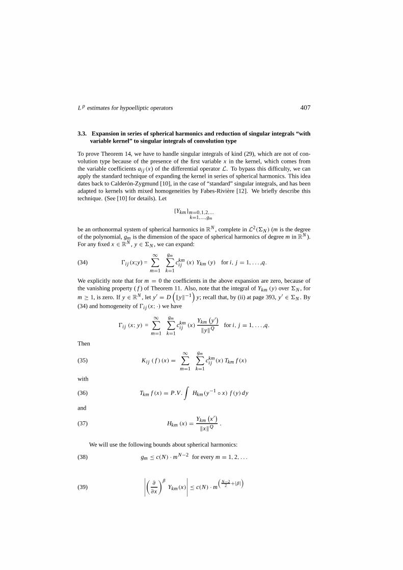
3.3. Expansion in series of spherical harmonics and reduction of singular integrals “withvariable kernel” to singular integrals of convolution type
To prove Theorem 14, we have to handle singular integrals of kind (29), which are not of con-volution type because of the presence of the first variablex in the kernel, which comes fromthe variable coefficientsai j (x) of the differential operatorL. To bypass this difficulty, we canapply the standard technique of expanding the kernel in series of spherical harmonics. This ideadates back to Calderon-Zygmund [10], in the case of “standard” singular integrals, and has beenadapted to kernels with mixed homogeneities by Fabes-Rivi`ere [12]. We briefly describe thistechnique. (See [10] for details). Let
{Ykm}m=0,1,2,...k=1,...,gm
be an orthonormal system of spherical harmonics inRN , complete inL2(6N) (m is the degreeof the polynomial,gm is the dimension of the space of spherical harmonics of degree m in RN ).For any fixedx ∈ RN , y ∈ 6N , we can expand:
(34) 0i j (x;y) =∞∑
m=1
gm∑
k=1
ckmi j (x) Ykm (y) for i, j = 1, . . . ,q.
We explicitly note that form = 0 the coefficients in the above expansion are zero, because ofthe vanishing property (f ) of Theorem 11. Also, note that the integral ofYkm (y) over6N , for
m ≥ 1, is zero. Ify ∈ RN , let y′ = D(‖y‖−1
)y; recall that, by (ii) at page 393,y′ ∈ 6N . By
(34) and homogeneity of0i j (x; ·) we have
0i j (x; y) =∞∑
m=1
gm∑
k=1
ckmi j (x)
Ykm(y′)
‖y‖Qfor i, j = 1, . . . ,q.
Then
(35) Ki j ( f ) (x) =∞∑
m=1
gm∑
k=1
ckmi j (x) Tkm f (x)
with
(36) Tkm f (x) = P.V.
∫Hkm(y−1 ◦ x) f (y) dy
and
(37) Hkm (x) =Ykm
(x′)
‖x‖Q.
We will use the following bounds about spherical harmonics:
(38) gm ≤ c(N) · mN−2 for everym = 1, 2, . . .
(39)
∣∣∣∣∣
(∂
∂x
)β
Ykm(x)
∣∣∣∣∣ ≤ c(N) · m
(N−2
2 +|β|)

408 M. Bramanti - L. Brandolini
for x ∈ 6N , k = 1, . . . , gm, m = 1, 2, . . ..
Moreover, if f ∈ C∞(6N ) and if f (x) ∼∑
k,m bkm Ykm(x) is the Fourier expansion of
f (x) with respect to{Ykm
}, that is
bkm =∫
6N
f (x) Ykm(x) dσ(x)
then, for every positive integerr there existscr such that
(40) |bkm| ≤ cr · m−2r supx∈6N|β|=2r
∣∣∣∣( ∂
∂x
)βf (x)
∣∣∣∣ .
In view of Theorem 12, we get from (40) the following bound on the coefficientsckmi j (x) ap-
pearing in the expansion (34): for every positive integerr there exists a constantc = c(r, G, µ)
such that
(41) supx∈RN
∣∣∣ckmi j (x)
∣∣∣ ≤ c(r, G, µ) · m−2r
for everym = 1, 2,. . .; k = 1, . . . , gm; i, j = 1, . . . , q.
3.4. Estimates on singular integrals of convolution type and their commutators, and con-vergence of the series
We now focus our attention on the singular integrals of convolution type defined by (36), (37)and their commutators. Our goal is to prove, for these operators, bounds of the kind (31), (32);moreover, we need to know explicitly the dependence of the constants on the indexesk, m,appearing in the series (35). To this aim, we apply some abstract results about singular integralsin spaces of homogeneous type, proved by Bramanti-Cerutti in [4]. To state precisely theseresults, we recall the following:
DEFINITION 1. Let X be a set and d: X × X → [0,∞). We say that d is a quasidistanceif it satisfies properties (9), (10), (11). The balls defined by d induce a topology in X; we assumethat the balls are open sets, in this topology. Moreover, we assume there exists a regular Borelmeasureµ on X, such that the “doubling condition” is satisfied:
µ (B2r (x)) ≤ c · µ (Br (x))
for every r > 0, x ∈ X, some constant c. Then we say that(X, d, µ) is a space of homogenoustype.
Let (X, d, µ) be an unbounded space of homogenous type. For every x∈ X, define
rx = sup{r > 0 : Br (x) = {x}}
(here sup∅ = 0). We say that(X, d, µ) satisfies a reverse doubling condition if there existc′ > 1, M > 1 such that for every x∈ X, r > rx
µ(BMr (x)) ≥ c′ · µ(Br (x)).

L p estimates for hypoelliptic operators 409
THEOREM 16. (See [4]). Let (X, d, µ) be a space of homogenous type and, if X is un-bounded, assume that the reverse doubling condition holds.Let k : X × X \ {x = y} → R be akernel satisfying:
i) the growth condition:
(42) |k(x, y)| ≤ c1
µ
(B (x, d(x, y))
) for every x, y ∈ X, some constant c1
ii ) the “Hormander inequality”: there exist constants c2 > 0, β > 0, M > 1 such that forevery x0 ∈ X, r > 0, x ∈ Br (x0), y /∈ BMr (x0),
|k(x0,y) − k(x, y)| + |k(y, x0) − k(y, x)| ≤
(43) ≤c2
µ
(B (x0, d(x0, y))
) ·d(x0,x)β
d(x0,y)β;
iii ) the cancellation property: there exists c3 > 0 such that for every r, R,0 < r < R < ∞,a.e. x
(44)
∣∣∣∣∫
r<d(x,y)<Rk(x, y) dµ(y)
∣∣∣∣+∣∣∣∣∫
r<d(x,z)<Rk(z, x) dµ(z)
∣∣∣∣ ≤ c3.
iv) the following condition: for a.e. x∈ X there exists
(45) limε→0
∫
ε<d(x,y)<1k(x, y) dµ(y).
For f ∈ Lp, p ∈ (1, ∞), set
Kε f (x) =∫
ε<d(x,y)<1/εk(x, y) f (y) dµ(y).
Then Kε f converges (strongly) inLp for ε → 0 to an operator K f satisfying
(46) ‖K f ‖p ≤ c‖ f ‖p for every f ∈ Lp,
where the constant c depends on X, p and all the constants involved in the assumptions.
Finally, for the operator K the commutator estimate holds:
(47) ‖C [K , a] f ‖p ≤ c‖a‖∗ ‖ f ‖p
for every f ∈ Lp, a ∈ BM O, and c the same constant as in(46).
REMARK 3. The constantc in (46), (47) has the following form:
c(p, X, β, M) · (c1 + c2 + c3).
Proof. To see this, note that ifk satisfies (42), (43), (44) with constantsc1, c2, c3, thenk′ ≡k/(c1 + c2 + c3) satisfies (42), (43), (44) with constants 1, 1, 1, so that for the kernelk′ c =c(p, X, β, M).

410 M. Bramanti - L. Brandolini
Let us apply Theorem 16 to our case. By (12), our space satisfies also the reverse doublingcondition. Consider the kernels:
k(x, y) = Hkm
(y−1 ◦ x
)with Hkm (x) =
Ykm(x′)
‖x‖Q.
By homogeneity,k satisfies (42) with
(48) c1 = c(G) · supx∈6N
|Ykm (x)| .
To check condition (43) we need the following:
PROPOSITION1. Let f ∈ C1(RN \ {0}
)be homogeneous of degreeλ < 1. There exist
c = c(G, f ) > 0, M = M(G) > 1 such that
(49) | f (x ◦ y) − f (x)| + | f (y ◦ x) − f (x)| ≤ c‖y‖ ‖x‖λ−1
for every x, y such that‖x‖ ≥ M ‖y‖. Moreover
c = c(G) · supz∈6N
|∇ f (z)| .
Proof. This proposition is essentially proved in [11], apart from the explicit form of the constantc.
ChooseM > 1 such that if‖x‖ = 1 and‖y‖ ≤ 1/M then‖x ◦ y‖ ≥ 1/2. Set:
F(x, y) = f (x ◦ y), L(x, y) = x ◦ y
andK ≡
{(x, y) : ‖x‖ = 1 and‖y‖ ≤ 1/M
}.
By homogeneity, it is enough to prove (49) for(x, y) ∈ K . Since f (z) is smooth for‖z‖ ≥ 1/2andL is smooth (everywhere), by the mean value theorem
| f (x ◦ y) − f (x)| = |F(x, y) − F(x, 0)| ≤ |y| ·∣∣∇F
(x, y∗)∣∣
with(x, y∗) ∈ K . But:
sup(x,y)∈K
∣∣∣∣∂F
∂xi(x, y)
∣∣∣∣ ≤N∑
j =1
sup(x,y)∈K
∣∣∣∣∂L j
∂xi(x, y)
∣∣∣∣ · sup‖z‖≥ 1
2
∣∣∣∣∂ f
∂z j(z)
∣∣∣∣ ≤
≤ c(G) · supz∈6N
|∇ f (z)| ,
and the same holds for sup(x,y)∈K
∣∣∣ ∂F∂yi
(x, y)
∣∣∣.Recalling that|y| ≤ c(G) ‖y‖ when‖y‖ ≤ 1 (see (8)), and repeating the argument for
| f (y ◦ x) − f (x)|, we get the result.
L p estimates for hypoelliptic operators 411
By Proposition 1,k satisfies (43), withβ = 1, M = M(G), and
(50) c2 = c(G) · supx∈6N
|∇Ykm (x)| .
As to (44), the left hand side equals:
∣∣∣∣∫
r<‖y‖<RHkm(y) dy
∣∣∣∣+∣∣∣∣∣
∫
r<∥∥y−1
∥∥<RHkm(y) dy
∣∣∣∣∣ .
The first term is a multiple of ∣∣∣∣∫
6N
Hkm(y) dσ (y)
∣∣∣∣
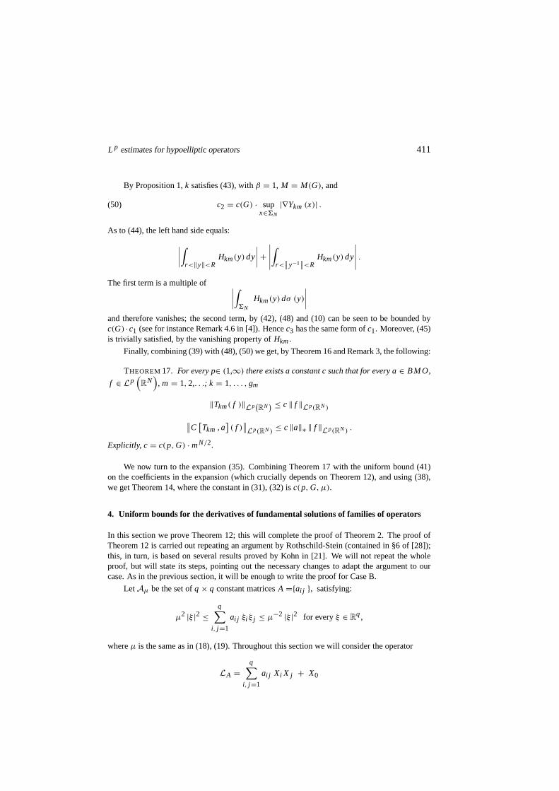
and therefore vanishes; the second term, by (42), (48) and (10) can be seen to be bounded byc(G) ·c1 (see for instance Remark 4.6 in [4]). Hencec3 has the same form ofc1. Moreover, (45)is trivially satisfied, by the vanishing property ofHkm.
Finally, combining (39) with (48), (50) we get, by Theorem 16and Remark 3, the following:
THEOREM17. For every p∈ (1,∞) there exists a constant c such that for every a∈ BM O,
f ∈ Lp(RN
), m = 1, 2,. . .; k = 1, . . . , gm
‖Tkm( f )‖Lp(RN
) ≤ c‖ f ‖Lp(RN)
∥∥C[Tkm , a
]( f )
∥∥Lp(RN)
≤ c‖a‖∗ ‖ f ‖Lp(RN) .
Explicitly, c= c(p, G) · mN/2.
We now turn to the expansion (35). Combining Theorem 17 with the uniform bound (41)on the coefficients in the expansion (which crucially depends on Theorem 12), and using (38),we get Theorem 14, where the constant in (31), (32) isc(p, G, µ).
4. Uniform bounds for the derivatives of fundamental solutions of families of operators
In this section we prove Theorem 12; this will complete the proof of Theorem 2. The proof ofTheorem 12 is carried out repeating an argument by Rothschild-Stein (contained in §6 of [28]);this, in turn, is based on several results proved by Kohn in [21]. We will not repeat the wholeproof, but will state its steps, pointing out the necessary changes to adapt the argument to ourcase. As in the previous section, it will be enough to write the proof for Case B.
LetAµ be the set ofq × q constant matricesA ={ai j }, satisfying:
µ2 |ξ |2 ≤q∑
i, j =1
ai j ξi ξ j ≤ µ−2 |ξ |2 for everyξ ∈ Rq,
whereµ is the same as in (18), (19). Throughout this section we will consider the operator
LA =q∑
i, j =1
ai j Xi X j + X0
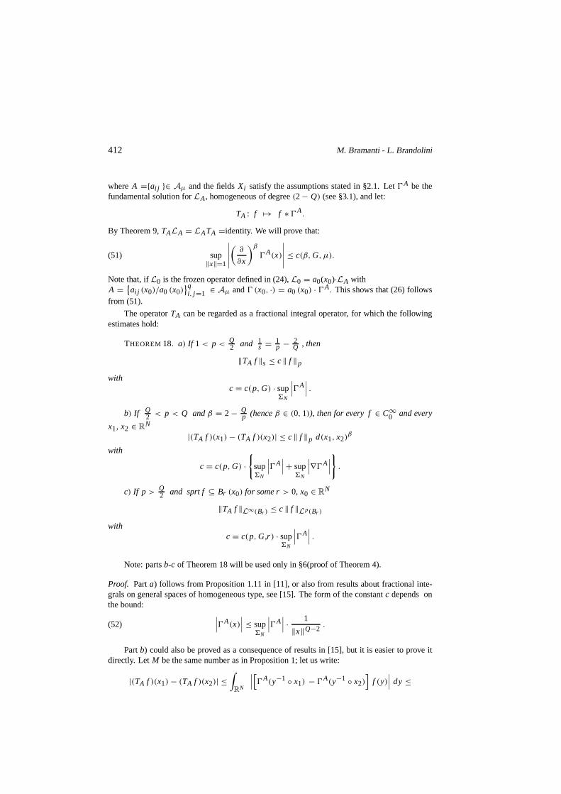
412 M. Bramanti - L. Brandolini
whereA ={ai j }∈ Aµ and the fieldsXi satisfy the assumptions stated in §2.1. Let0A be thefundamental solution forLA, homogeneous of degree(2 − Q) (see §3.1), and let:
TA : f 7→ f ∗ 0A.
By Theorem 9,TALA = LATA =identity. We will prove that:
(51) sup‖x‖=1
∣∣∣∣∣
(∂
∂x
)β
0A(x)
∣∣∣∣∣ ≤ c(β, G, µ).
Note that, ifL0 is the frozen operator defined in (24),L0 = a0(x0)·LA withA =
{ai j (x0)/a0 (x0)
}qi, j =1 ∈ Aµ and0 (x0, ·) = a0 (x0) · 0A. This shows that (26) follows
from (51).
The operatorTA can be regarded as a fractional integral operator, for whichthe followingestimates hold:
THEOREM18. a) If 1 < p <Q2 and 1
s = 1p − 2
Q , then
‖TA f ‖s ≤ c‖ f ‖p
withc = c(p, G) · sup
6N
∣∣∣0A∣∣∣ .
b) If Q2 < p < Q andβ = 2 − Q
p (henceβ ∈ (0, 1)), then for every f∈ C∞0 and every
x1, x2 ∈ RN
|(TA f )(x1) − (TA f )(x2)| ≤ c‖ f ‖p d(x1, x2)β
with
c = c(p, G) ·{
sup6N
∣∣∣0A∣∣∣+ sup
6N
∣∣∣∇0A∣∣∣}
.
c) If p >Q2 and sprt f ⊆ Br (x0) for some r> 0, x0 ∈ RN
‖TA f ‖L∞(Br ) ≤ c‖ f ‖Lp(Br )
withc = c(p, G,r) · sup
6N
∣∣∣0A∣∣∣ .
Note: partsb-c of Theorem 18 will be used only in §6(proof of Theorem 4).
Proof. Parta) follows from Proposition 1.11 in [11], or also from resultsabout fractional inte-grals on general spaces of homogeneous type, see [15]. The form of the constantc depends onthe bound:
(52)∣∣∣0A(x)
∣∣∣ ≤ sup6N
∣∣∣0A∣∣∣ · 1
‖x‖Q−2.
Partb) could also be proved as a consequence of results in [15], butit is easier to prove itdirectly. LetM be the same number as in Proposition 1; let us write:
|(TA f )(x1) − (TA f )(x2)| ≤∫
RN
∣∣∣[0A(y−1 ◦ x1) − 0A(y−1 ◦ x2)
]f (y)
∣∣∣ dy ≤

L p estimates for hypoelliptic operators 413
≤∫∥∥y−1◦x1
∥∥≥M∥∥∥x−1
2 ◦x1
∥∥∥. . . dy +
∫∥∥y−1◦x1
∥∥≤M∥∥∥x−1
2 ◦x1
∥∥∥. . . dy = I + I I .
By Proposition 1,
I ≤ c(p, G) · sup6N
∣∣∣∇0A∣∣∣∥∥∥x−1
2 ◦ x1
∥∥∥∫∥∥y−1◦x1
∥∥≥M∥∥∥x−1
2 ◦x1
∥∥∥
| f (y)|∥∥y−1 ◦ x1
∥∥Q−1dy.
Let p, p′ be conjugate exponents; by Holder’s inequality and a change of variables
I ≤ c∥∥∥x−1
2 ◦ x1
∥∥∥ ‖ f ‖p
∫
‖y‖≥M∥∥∥x−1
2 ◦x1
∥∥∥
1
‖y‖(Q−1)p′ dy
1/p′
≤
computing the integral, under the assumptionp < Q,
≤ c∥∥∥x−1
2 ◦ x1
∥∥∥β
‖ f ‖p
whereβ = 1 − 1q [(Q − 1)(q − 1) − 1] = 2 − Q
p ∈ (0, 1).
By (52),
I I ≤ sup6N
∣∣∣0A∣∣∣ ·
·∫∥∥y−1◦x1
∥∥≤M∥∥∥x−1
2 ◦x1
∥∥∥| f (y)|
{1
∥∥y−1 ◦ x1∥∥Q−2
+ 1∥∥y−1 ◦ x2
∥∥Q−2
}dy =
= I I ′ + I I ′′.
By Holder’s inequality and reasoning as above, we get, ifp > Q/2,
I I ′ ≤ c∥∥∥x−1
2 ◦ x1
∥∥∥β
‖ f ‖p .
As to I I ′′, if∥∥∥y−1 ◦ x1
∥∥∥ ≤ M∥∥∥x−1
2 ◦ x1
∥∥∥, then∥∥∥y−1 ◦ x2
∥∥∥ ≤ c∥∥∥x−1
2 ◦ x1
∥∥∥ and thereforeI I ′′
can be handled asI I ′.As to c), noting thatx, y ∈ Br (x0) ⇒ y−1 ◦ x ∈ BKr (0) for someK = K (G), we can
write, by Holder’s inequality (letp′ be the conjugate exponent ofp):
‖TA f ‖L∞(Br (x0))≤ ‖ f ‖Lp(Br (x0))
·∥∥∥0A
∥∥∥Lp′
(BKr (0))≤ (by (52))
≤ ‖ f ‖Lp(Br (x0))· c(p, G) · sup
6N
∣∣∣0A∣∣∣ · r 2−Q/p,
which proves the result, assumingp > Q/2.
Now, letSA
i j f = Xi X j TA f.
By (c) of Theorem 11, setting0Ai j = Xi X j 0
A, we can write
(53) SAi j f = P.V.
(0A
i j ∗ f)
+ αi j (A) · f.
Let us apply Theorem 16 and Remark 3 to the kernel0Ai j . By the properties (d), (e), ( f ) listed
in Theorem 11 and Proposition 1, we get:

414 M. Bramanti - L. Brandolini
THEOREM19. For every p∈ (1, ∞), f ∈ C∞0
(RN
),
∥∥∥P.V.
(0A
i j ∗ f)∥∥∥
p≤ c‖ f ‖p
with
c = c(p, G) ·{
sup6N
∣∣∣0A∣∣∣+ sup
6N
∣∣∣∇0A∣∣∣}
.
LEMMA 2. For every p∈ (1,∞) and for every A0 ∈ Aµ, there existsε > 0 such that if|A − A0| < ε, then
‖EA f ‖p ≤ 1
2‖ f ‖p
where|A| denotes the Euclidean norm of the matrix A and
EA =(LAo − LA
)TAo .
This Lemma is proved in [28] (Lemma 6.5), for a different class of operators.
Proof. Let us write
LAo − LA =q∑
i, j =1
(ao
i j − ai j
)Xi X j .
Then
EA f =q∑
i, j =1
(ao
i j − ai j
)Xi X j TAo f.
By (53) and Theorem 19 we get the result.
LEMMA 3. Let p ∈ (1, Q/2) and let 1s = 1
p − 2Q . There exists c= c(G, µ, p) such that
for every A∈ Aµ
(54) ‖TA f ‖s ≤ c‖ f ‖p .
This Lemma is an adjustment of Lemma 6.7 proved in [28], whichcontains a minor mistake(it implicitly assumesQ > 4).
Proof. Let A0 ∈ Aµ and letEA andε be as in the previous lemma. For everyf ∈ Lp, if|A − A0| < ε, then for everyp ∈ (1, ∞), ‖EA f ‖p ≤ 1
2 ‖ f ‖p , so that we can write
(55)∞∑
n=0
(En
A)
f = (I − EA)−1 f ≡ g.
Thereforef = (I − EA)g = g − LAo TAo g + LATAo g = LATAo g,
that isTA f = TAo g.

L p estimates for hypoelliptic operators 415
Again from (55) we have
‖g‖p ≤∞∑
n=0
‖EA‖n ‖ f ‖p = 2‖ f ‖p ,
hence by Theorem 18.a, if p, s are as in the statement of the theorem,
‖TA f ‖s =∥∥TAo g
∥∥s ≤ c(G, p, A0) ‖g‖p ≤ 2c‖ f ‖p .
Since this is true for every fixedA0 ∈ Aµ and any matrixA such that|A − A0| < ε, by the
compactness ofAµ in Rq2we can choose a constantc = c(G, p,µ) such that (54) holds for
everyA ∈ Aµ.
THEOREM 20. Let ϕ, ϕ1 ∈ C∞0
(RN
)with ϕ1 = 1 on sprtϕ. There existsε = ε (G)
and, for every t∈ R, there exists c= c(t, µ,G, ϕ, ϕ1) such that for every A∈ Aµ and every
u ∈ C∞0
(RN
)
‖ϕu‖H t+ε,2 ≤ c{‖ϕ1LAu‖H t,2 + ‖ϕ1u‖
L2}.
(Recall that the norm of Ht,2(RN
)has been defined is §2.3).
This Theorem is proved in [21] for a different class of operators and without taking intoaccount the exact dependence of the constant on the parameters. To point out the slight modi-fications which are necessary to adapt the proof to our case, we will state the main steps of theproof of Theorem 20. Before doing this, however, we show how from Lemma 3 and Theorem20, the uniform bound (26) follows. This, again, is an argument contained in [28], which weinclude, for convenience of the reader, to make more readable the exposition. Moreover, a minorcorrection is needed here to the proof of [28].
Proof of (26) from Lemma 3 and Theorem 20.Throughout the proof,Br will be a ball centered
at the origin. Letg ∈ C∞0 (B2 \ B1) such that‖g‖2 ≤ 1, and letϕ, ϕ1 ∈ C∞
0
(RN
)such that:
ϕ = 1 in B1/4, sprtϕ ⊆ B1/2, ϕ1 = 1 in B1/2, sprtϕ1 ⊆ B1. Let f = TAg. SinceLA f = g = 0in B1 andLA is hypoelliptic, f ∈ C∞ (B1).
Pick a positive numberp such that max(
12, 2
Q
)< 1
p < min(
12 + 2
Q , 1)
and lets be as in
Lemma 3. Note that 1< p < Q/2 andp < 2 < s. Then, by Lemma 3:
‖ϕ1 f ‖2 ≤ c(ϕ1) ‖ f ‖s ≤ c(ϕ1,G, µ, p) ‖g‖p ≤ c(ϕ1,G, µ) ‖g‖2 ≤ c(ϕ1,G, µ).
Applying Theorem 20 toϕ, ϕ1, f , sinceLA f = 0 on sprtϕ1, we get:
‖ϕ f ‖H t+ε,2 ≤ c ‖ϕ1 f ‖2 ≤ c(t ,ϕ,ϕ1,G, µ)
for everyt ∈ R. Therefore, by the standard Sobolev embedding Theorems, wecan bound any(isotropic) Holder normCh,α of f on B1/4 with a constantc(h, G, µ); in particular, for everydifferential operatorP:
(56) |P f (0)| ≤ c(P, G, µ).

416 M. Bramanti - L. Brandolini
Now, recall thatf = g ∗ 0A. If P is any left invariant differential operator,
(57) P f (0) =∫
P 0A(y−1) g(y) dy.
Since (56) holds for everyg ∈ C∞0 (B2 \ B1) such that‖g‖2 ≤ 1, from (57) we get
(58)∥∥∥P 0A(y−1)
∥∥∥L2(B2\B1)
≤ c(P, G, µ).
Now, writing any differential operator(
∂∂x
)βin terms of left invariant vector fields, (58) gives
us a bound on everyHk,2-norm of0A on B2 \ B1, and therefore, reasoning as above, on everyHolder normCh,α of 0A on a smaller spherical shellC ≡ B7/4 \ B5/4. In particular, we get
supx∈C
∣∣∣∣∣
(∂
∂x
)β
0A(x)
∣∣∣∣∣ ≤ c(β, G, µ),
from which (51) follows, by homogeneity of0A.
Now we come to Theorem 20, which is proved by Kohn in [21] for anoperator of the kind
Pu ≡q∑
i=1
X2i u + X0u + cu,
where the fieldsXi (i = 0, 1, . . . , q) satisfy Hormander’s condition. Reading carefully thepaper [21], one can check that the whole proof can be repeatedreplacing the operatorP withLA; moreover, the constants depend on the matrixA only through the numberµ. Actually,the matrixA is involved in the proof only through the boundedness of its coefficients and thefollowing elementary inequality:
|(LAu, u)| ≥ µ
q∑
i=1
‖Xi u‖2 , for everyu ∈ C∞0
(R
N)
.
We can rephrase as follows the steps of the proof of Theorem 20given in [21]:
(i) There existε = ε(G), c = c(G, µ) such that for everyu ∈ C∞0
(RN
)and everyA ∈ Aµ
‖u‖Hε,2 ≤ c{‖LAu‖2 + ‖u‖2
}.
(ii ) For everyt ∈ R, M > 0, there existsc = c(t, M, µ, G) such that for everyu ∈C∞
0
(RN
)and everyA ∈ Aµ
‖u‖H t+ε,2 ≤ c{‖LAu‖H t,2 + ‖u‖H−M,2
},
whereε is the same of (i).
(iii ) (Localization of the above estimate).
‖ϕu‖H t+ε,2 ≤ c{‖ϕ1LAu‖H t,2 + ‖ϕ1u‖H−M,2
},
whereϕ, ϕ1 ∈ C∞0
(RN
)with ϕ1 = 1 on sprtϕ, c = c(ϕ,ϕ1,t, M, µ, G).
Since‖·‖H−M,2 ≤ ‖·‖2 , from point (iii) we get Theorem 20.

L p estimates for hypoelliptic operators 417
REMARK 4 (AN ALGEBRA OF PSEUDODIFFERENTIAL OPERATORS
ADAPTED TO THE FIELDSXi ).For the reader who is interested in reviewing the proof of [21], we point out that, under ourassumptions, many of the arguments of [21] can be simplified and made more self-contained bythe following remark. We can precisely define an algebra of pseudodifferential operators, actingon the Schwarz’ spaceS of smooth functions with fast decay at infinity. Consider thefollowingkinds of operators:
(a) multiplication by a polynomial;
(b) Xi (i = 0, 1, . . . , q);
(c) for t ∈ R, 3t defined by(3t u
)(ξ) =
(1 + |ξ |2
)t/2u(ξ).
By general properties of homogeneous groups (see [31], p. 621), the vector fieldsXi arelinear combinations of∂/∂xi with polynomial coefficients (and, by Hormander’s condition, the∂/∂xi ’s are linear combinations of theXi ’s and their commutators, with polynomial coefficients).ThereforeXi mapsS into itself, while the same is true for the operators (a) and (c). The transposeof an operator of kind (a), (c) is the operator itself, while,since the fieldsXi are translationinvariant, the transpose ofXi is −Xi . (This fact also simplifies many of the arguments in [21];in particular, note that(X0u, u) = 0). LetP be the algebra generated by operators (a), (b), (c)under sums, composition and transpose. This algebra is the suitable context where the wholeproof can be carried out. On the contrary, in [21] some technical problems arise, sinceXi are
defined only onC∞0
(RN
).
To complete the proof of Theorem 12 we have now to prove estimate (27). We actuallyprove a more general result which will be useful in §6.
Let{kγ
}γ∈3
be a family of kernels such thatkγ is homogeneous of degreeh− Q for some
h > 0 andkγ ∈ C∞0
(RN \ {0}
). Let Tγ be the distribution associated tokγ and letPh be a
left invariant differential operator homogeneous of degree h. Then, Theorem 9 states that
(59) PhTγ = P.V.(
Phkγ
)+ αγ δ.
(Observe that (25) is a particular case of (59)). With these notations, we can prove the following:
LEMMA 4. If kγ satisfies a uniform bound like (26), that is, for every multiindexβ
supγ∈3
sup‖y‖=1
∣∣∣∣∣
(∂
∂y
)β
kγ (y)
∣∣∣∣∣ ≤ c (β) ,
thensupγ∈3
∣∣αγ
∣∣ ≤ c.
Proof. Let u be a test function withu(0) 6= 0, sprtu ⊆ B1 (0). By (59)
αγ u(0) = 〈 (Ph)T u, Tγ 〉 − 〈u, P.V.(
Phkγ
)〉 =
=∫
(Ph)T u(x) kγ (x) dx − limε→0
∫
‖x‖>εPhkγ (x) u(x) dx

418 M. Bramanti - L. Brandolini
(here (·)T denotes transposition). Sincekγ is locally integrable, the first integral is bounded,uniformly in γ by (59). As to the second term, by the vanishing property of the kernelPhkγ
(see Lemma 1), homogeneity and (59) we can write∣∣∣∣∫
‖x‖>εPhkγ (x) u(x) dx
∣∣∣∣ =∣∣∣∣∫
ε<‖x‖<1Phkγ (x) [u(x) − u(0)] dx
∣∣∣∣ ≤
≤ sup‖y‖≤1
|∇u(y)|∫
ε<‖x‖<1
c
‖x‖Q· |x| dx ≤ c.
(The convergence of the last integral follows from (8)).
5. Some properties of the Sobolev spacesSk,p
We start pointing out the following interpolation inequality for Sobolev norms:
PROPOSITION2. Let X be a left invariant vector field, homogeneous of degreeα > 0. Then
for everyε > 0, u ∈ Sp(RN
), p ∈ [1, ∞)
(60) ‖Xu‖p ≤ ε
∥∥∥X2u∥∥∥
p+ 2
ε‖u‖p .
Proof. The following argument is taken from the proof of Theorem 9.4in [13]. Let γ (t) be theintegral curve ofX with γ (0) = 0. Then, applying Taylor’s theorem to the functionF(t) =u (x ◦ γ (t)),
u(x ◦ γ (1) ) = u(x) + Xu(x) +∫ 1
0(1 − t) X2u(x ◦ γ (t))dt.
Using the translation invariance of‖·‖p and Minkowski’s inequality, we get
‖Xu‖p ≤∥∥∥X2u
∥∥∥p
+ 2‖u‖p .
SinceX is homogeneous, by a dilation argument we get the result.
We will need a version of (60) for functions defined on a ball (not necessarily vanishing atthe boundary). For standard Sobolev norms, this result follows from the analog of (60) using anextension theorem (see for instance [14], pp. 169-173). However, it seems not easy to constructa continuous extension operatorE: Sp (Br ) → Sp
0 (B2r ). We are going to show how to bypassthis difficulty.
First we construct a suitable family of cutoff functions. Given two ballsBr1, Br2 and a
functionϕ ∈ C∞0
(RN
), let us writeBr1 ≺ ϕ ≺ Br2 to say that 0≤ ϕ ≤ 1, ϕ ≡ 1 on Br1 and
sprtϕ ⊆ Br2.
LEMMA 5 (RADIAL CUTOFF FUNCTIONS). For anyσ ∈ (0, 1), r > 0, k positive integer,
there existsϕ ∈ C∞0
(RN
)with the following properties:
Bσ r ≺ ϕ ≺ Bσ ′r with σ ′ = (1 + σ) /2;

L p estimates for hypoelliptic operators 419
∣∣∣P j ϕ∣∣∣ ≤ c(G, j )
σ j −1 (1 − σ) j r jfor 1 ≤ j ≤ k,
where Pj is any left invariant differential monomial homogeneous ofdegree j .
Proof. For simplicity, we prove the assertion fork = 2. The general case is similar. Pick afunction f : [0, r ) → [0, 1] such that:
f ≡ 1 in [0, σ r ), f ≡ 0 in [σ ′r, r ), f ∈ C∞ (0, r ) ,
∣∣ f ′∣∣ ≤c
(1 − σ) r,∣∣ f ′′∣∣ ≤
c
(1 − σ)2 r 2.
Setting ϕ(x) = f (‖x‖), we can compute:
Xi ϕ(x) = f ′(‖x‖)Xi (‖x‖) ;
Xi X j ϕ (x) = f ′′(‖x‖)Xi (‖x‖) X j (‖x‖) + f ′(‖x‖)Xi X j (‖x‖) .
SinceXi (‖x‖) is homogeneous of degree zero fori = 1, . . . , q, Xi X j (‖x‖)(for i, j = 1, . . . , q) andX0 (‖x‖) are homogeneous of degree−1 and f ′(‖x‖) 6= 0 for ‖x‖ >
σ r , we get the result.
Another tool we need in this context is an approximation result by suitable mollifiers. For afixed cutoff functionϕ, B1 (0) ≺ ϕ ≺ B2 (0), set, for everyε > 0,
ϕε(x) = c · ε−Q ϕ
(D
(1
ε
)x
)
with c =(∫
RN ϕ(x) dx)−1. Then
LEMMA 6. For u ∈ Sk,p(RN
)(k nonnegative integer, 1≤ p < ∞) and ϕε as above,
define uε = ϕε ∗ u. Then uε ∈ C∞ and uε → u in Sk,p for ε → 0.
Proof. The proof follows the same line as in the Euclidean case. We just point out the followingfacts:
(i) convergence inLp is established first foru ∈ 3β (G,RN), u with bounded support.The density of this space inLp can be proved in a general space of homogeneous type (see forinstance [4]);
(ii) sinceXi is right invariant,Xi (uε) =(
Xi u)ε: from this remark and convergence inLp
we get convergence inSk,p;
(iii ) to see thatuε ∈ C∞, one has to consider right invariant vector fieldsXRi , write
XRi (ϕε ∗ u) =
(XR
i ϕε
)∗u, and iterate. The possibility of representing any Euclidean derivative
in terms of right invariant vector fields (see §2.5) providesthe conclusion.
The above Lemma is useful for us mainly in view of the following
COROLLARY 1. If u ∈ Sk,p (�) (1 ≤ p < ∞, k ≥ 1) and ϕ ∈ C∞0 (�), then uϕ ∈
Sk,p0 (�).

420 M. Bramanti - L. Brandolini
Proof. The functionuϕ is compactly supported in� and, extended to zero outside�, belongs to
Sk,p(RN
). Then(uϕ)ε converges touϕ in Sk,p. Since, forε small enough,(uϕ)ε is compactly
supported in�, (uϕ)ε ∈ C∞0 (�) anduϕ ∈∈ Sk,p
0 (�).
THEOREM21 (INTERPOLATION INEQUALITY IN CASE A). Assume we are in Case A. Forany u∈ SH,p(Br ), p ∈ [1, ∞), H ≥ 2, r > 0, define the following quantities:
8k = sup12<σ<1
((1 − σ)kr k
∥∥∥Dku∥∥∥Lp(Brσ )
)for k = 0, 1, 2, . . . , H.
Then for every integer j ,1 ≤ j ≤ H − 1, there exist positive constants c, δ0 depending onG, j, H such that for everyδ ∈ (0, δ0) we have
(61) 8 j ≤ δ 8H + c
δ j /(H− j )80.
Proof. We proceed by induction onH . Let H = 2.
Let u ∈ Sp(Br ) andϕ a cutoff function as in Lemma 5. By Corollary 1,uϕ ∈ Sp0 (Br ),
hence by density we can apply Proposition 2, writing
‖Xi (uϕ)‖p ≤ ε{‖ϕ Xi Xi u‖p + ‖2 Xi u Xi ϕ‖p + ‖u Xi Xi ϕ‖p
}+ 2
ε‖ϕu‖p
for anyε > 0. Hence
‖Du‖Lp(Bσ r ) ≤ ε
{∥∥∥D2u∥∥∥Lp(Bσ ′r )
+c(G)
(1 − σ) r‖Du‖Lp(Bσ ′r )
+
+c(G)
σ (1 − σ)2 r 2‖u‖Lp(Bσ ′r )
}+
2
ε‖u‖Lp(Bσ ′r )
.
Multiplying both sides for(1 − σ) r and choosingε = δσ (1 − σ) r we find
(1 − σ) r ‖Du‖Lp(Bσ r ) ≤ δσ (1 − σ)2 r 2∥∥∥D2u
∥∥∥Lp(Bσ ′r )
+
+c(G)δσ (1 − σ) r ‖Du‖Lp(Bσ ′r )+ c(G)
(δ + 1
δσ
)‖u‖Lp(Bσ ′r )
≤
(noting that (1− σ ′) = (1 − σ )/2)
≤ 4δ82 + C(G)δ81 + c(G)
(δ +
2
δ
)80.
Therefore
81 ≤ 4δ
1 − c(G)δ82 +
c(G)(δ + 2
δ
)
1 − c(G)δ80
which, forδ small enough, is equivalent to
(62) 81 ≤ δ82 + c
δ80.
Assume now that (61) holds forH − 1. An argument similar to that used to obtain (62) appliedto DH−2u yields
8H−1 ≤ δ8H + c
δ8H−2

L p estimates for hypoelliptic operators 421
while, by induction,
8H−2 ≤ η8H−1 +c
ηH−280.
Therefore
8H−1 ≤ δ8H +c
δ
(η8H−1 +
c
ηH−280
)
and, choosingη = δ2c we get
(63) 8H−1 ≤ 2δ8H + c
δH−180.
If j = H − 1, this is exactly what we have to prove; ifj < H − 1, by induction
8 j ≤ ε8H−1 + c
ε j /(H−1− j )80 ≤ by (63)
≤ ε
(2δ8H + c
δH−180
)+ c
ε j /(H−1− j )80.
Choosing 2δ = η1/(H− j ) andε = η1−1/(H− j ) we get the result.
REMARK 5. Note that the second part of the above proof does not hold inCase B since in
that caseDku cannot be obtained asD(
Dk−1u). However, the proof forH = 2 holds also in
Case B, since the fieldX0 does not play any role in the definition ofDu. We are going to provean analogous interpolation inequality, in Case B, which will hold for H even. This proof will beachieved in several steps.
Let
L ≡q∑
i=1
X2i + X0,
and let0 be the fundamental solution ofL homogeneous of degree two; recall that the transposeof L is just
LT ≡q∑
i=1
X2i − X0.
LEMMA 7. Let Q > 4. For every integer k≥ 2 and any couple of left invariant differentialmonomials P2k−1 and P2k−2, homogeneous of degrees2k − 1 and 2k − 2, respectively, wecan determine two kernels K(1), K (2) (depending only on these monomials) which are smoothoutside the origin and homogeneous of degrees(1 − Q) , (2 − Q), respectively, such that forany test function u
P2k−1u(x) =(
(L L . . . Lu)k times
∗ K (1)
)(x);
(64) P2k−2u(x) =(
(L L . . . Lu)k times
∗ K (2)
)(x).
Proof. By induction onk. Let k = 2. By Lemma 1, we can write
u = Lu ∗ 0 = (L Lu ∗ 0) ∗ 0 = L Lu ∗ K ,

422 M. Bramanti - L. Brandolini
whereK = 0 ∗ 0 is homogeneous of degree(4 − Q). Hence
P3u = L Lu ∗ P3K = L Lu ∗ K (1); P2u = L Lu ∗ P2K = L Lu ∗ K (2),
with K (1), K (2) homogeneous of degree(1 − Q), (2 − Q), respectively.
Now, assume (64) holds fork − 1, that is
P2k−3u(x) =(
(L L . . . Lu)(k−1) times
∗ K (1)
)(x);
P2k−4u(x) =(
(L L . . . Lu)(k−1) times
∗ K (2)
)(x).
Any differential monomialP2k−2 can be written either asXi P2k−3 (for somei = 1, . . . , q) orasX0 P2k−4. In the first case, we can write
P2k−2 u(x) = Xi
((L L . . . Lu)(k−1) times
∗ K (1)
)(x) =
= Xi
((L L . . . Lu)
k times∗(0 ∗ K (1)
))(x) =
=(
(L L . . . Lu)k times
∗ Xi
(0 ∗ K (1)
))(x) =
((L L . . . Lu)
k times∗ K (2)
)(x),
with K (2) homogeneous of degree((2 − Q) + (1 − Q) + Q) − 1 = 2 − Q (we have appliedLemma 1). In the second case,
P2k−2 u(x) = X0
((L L . . . Lu)(k−1) times
∗ K (2)
)(x) =
=(
(L L . . . Lu)k times
∗ X0
(0 ∗ K (2)
))(x) =
((L L . . . Lu)
k times∗ ˜K (2)
)(x),
with, again,˜K (2)homogeneous of degree (2− Q).
Similarly, any differential monomialP2k−1 can be written either asP2 P2k−3 (with P2 =X0 or P2 = Xi X j for somei, j = 1, . . . , q) or as P3 P2k−4 (with P3 = Xi X0 for somei = 1, . . . , q). Reasoning as above we get the result for this case, too.
LEMMA 8. For every integer k≥ 2 there exists a constant c(G, k) such that for everyε > 0and every test function u,
∥∥∥D2k− j u∥∥∥
p≤ ε
∥∥∥D2ku∥∥∥
p+ c(G, k)
ε2k− j‖u‖p for j = 1, 2, k ≥ 2.

L p estimates for hypoelliptic operators 423
Proof. Let K (1), K (2) be as in Lemma 7. We split the kernelK (1) as
K (1) = ϕK (1) + (1 − ϕ) K (1) ≡ K (1)0 + K (1)
∞ ,
whereϕ is a cutoff function,B1(0) ≺ ϕ ≺ B2(0). ThereforeK (1)0 is homogeneous of degree
(1 − Q) near the origin and has compact support, hence it is integrable, while K (1)∞ is homoge-
neous of degree(1 − Q) near infinity and vanishes near the origin. Writingf (x) = f (x−1), wecan compute
∫K (1)
∞(
y−1 ◦ x)
L L . . . Lu(y) dy =∫
K (1)∞(
x−1 ◦ y)
L L . . . Lu(y) dy =
=∫
LT K (1)∞ (x−1 ◦ y) (L L . . . L)
k−1 timesu(y) dy = . . .
=∫ (
LT LT . . . LT)
k times
K (1)∞(
x−1 ◦ y)
u(y) dy =
= u ∗
(
LT LT . . . LT)
k times
K (1)∞
∼
(x) ≡(u ∗ K (1)
1
)(x).
ThereforeP2k−1u(x) =
((L L . . . L)
k timesu ∗
[K (1)
0 + K (1)∞])
(x) =
= (L L . . . Lu) ∗ K (1)0 + u ∗ K (1)
1 ,
whereK (1)1 is homogeneous of degree(1 − Q − 2k) near infinity and vanishes near the origin,
hence it is integrable. Integrability ofK (1)0 , K (1)
1 gives
∥∥∥D2k−1u∥∥∥
p≤ c(G, k)
{∥∥∥D2ku∥∥∥
p+ ‖u‖p
}.
The same reasoning applied toK (2) gives∥∥∥D2k−2u
∥∥∥p
≤ c(G, k)
{∥∥∥D2ku∥∥∥
p+ ‖u‖p
}.
The conclusions follows from the last two inequalities and adilation argument.
THEOREM22. [Interpolation inequality in Case B] For any functionu ∈ S2k,p(Br ) (k ≥ 1, p ∈ [1, ∞), r > 0), let 8h (h = 0, 1, . . . , 2k) be the seminorms definedin Theorem 21. Then
8 j ≤ ε82k + c(ε, k)80
for every integer j with1 ≤ j ≤ 2k − 1 and everyε > 0.
Proof. Let ϕ be a cutoff function as in Lemma 5. By Corollary 1uϕ ∈ S2k,p0 (Br ), hence, by
density, we can apply Lemma 8 touϕ. By standard arguments (see the first part of the proof ofTheorem 21) we get, for everyδ > 0,
82k− j ≤ δ
2k∑
h=0
8h +c
δ(2k− j )/ j80 ( j = 1, 2).

424 M. Bramanti - L. Brandolini
The previous inequality clearly holds ifk is replaced by any integeri with 2 ≤ i ≤ k. Addingup these inequalities for 2≤ i ≤ k, j = 1, 2, we get
k∑
i=2
(82i−1 + 82i−2
)=
2k−1∑
i=2
8i ≤ 2δ
k∑
i=2
2i∑
h=0
8h
+ c(δ, k) · 80 ≤
≤ 2δk2k∑
h=0
8h + c(δ, k) · 80.
Adding also (62) (which holds in Case B, too, as noted in Remark 5):
81 ≤ δ82 + c
δ80
we can write2k−1∑
h=0
8h ≤ 2δk2k∑
h=0
8h + c(δ, k) · 80
and, finally, for everyε > 0,
2k−1∑
h=0
8h ≤ ε · 82k + c(ε, k) · 80
which proves the result.
Next, we need the following Sobolev-type embedding theorem:
THEOREM23. Let u ∈ Sp0 (Br ) for some r> 0. Then:
a) if 1 < p <Q2 and 1
p∗ = 1p − 2
Q , then
‖u‖p∗ ≤ c (p, G)
∥∥∥D2u∥∥∥
p;
b) if Q2 < p < Q andβ = 2 − Q
p , then
‖u‖3β (Br )≤ c(p, G, r )
∥∥∥D2u∥∥∥Lp(Br )
.
Proof. Let L , 0 be as in the proof of Lemma 7. Then for anyu ∈ C∞0 (Br ) we can write
u = Lu ∗ 0.
Theorem 18 then gives the assertion.
The results contained in Theorem 23 have been proved by Folland in [11], where a morecomplete theory of Sobolev and Holder spaces defined by the vector fieldsXi is developed (see§§4, 5 in [11], in particular Theorems 4.17 and 5.15). However, Folland’s theory relies on a deepanalysis of the sub-Laplacian on stratified groups, and therefore does not cover completely thecases we are considering here: remember that under our assumptions, the groupG is graded butnot necessarily stratified.

L p estimates for hypoelliptic operators 425
6. Local estimates for solutions to the equationLu = f in a domain
In this section we will prove Theorems 3 to 7, as a consequenceof the basic estimate containedin Theorem 2 and the properties of Sobolev spaces expounded in §5. For convenience of thereader, we recall the statement of each Theorem before its proof.
THEOREM 3 (LOCAL Lp-ESTIMATES FOR SOLUTIONS TO THE EQUATIONLu = f IN
A DOMAIN ). Under the assumptions stated in §2.3, let� be a bounded domain ofRN and�′ ⊂⊂ �. If u ∈ Sp (�), then
‖u‖Sp(�′) ≤ c{‖Lu‖Lp(�) + ‖u‖Lp(�)
}
where c= c(p, G, µ, η, �,�′).
Proof of Theorem 3.Let u ∈ Sp (�), Br ⊂ �, and fix r0 = r0 (p, G, µ, η) in such a waythat for r < r0 Theorem 2 holds. Letϕ be a cutoff function as in Lemma 5. By Corollary 1,uϕ ∈ Sp
0 (Br ); then, by density, we can apply Theorem 2 touϕ:
∥∥Xi X j (uϕ)∥∥
p ≤ c‖L (uϕ)‖p .
From the above inequality we get:
∥∥Xi X j u∥∥Lp(Bσ r )
≤ c{‖Lu‖Lp(Bσ ′r )
+c(G)
(1 − σ) r‖Du‖Lp(Bσ ′r )
+
+c(G)
σ (1 − σ)2 r 2‖u‖Lp(Bσ ′r )
}.
Multiplying both sides for(1 − σ)2 r 2, adding to both sides(1 − σ) r ‖Du‖Lp(Bσ r ), reasoninglike in the first part of the proof of Theorem 21 and applying (62) we get
82 + 81 ≤ c{r 2 ‖Lu‖Lp(Br ) + ‖u‖Lp(Br )
}.
Hence
r 2∥∥∥D2u
∥∥∥Lp(Br/2
) + r ‖Du‖Lp(Br/2
) ≤ c{r 2 ‖Lu‖Lp(Br ) + ‖u‖Lp(Br )
},
that is‖u‖Sp(Br/2) ≤ c
{‖Lu‖Lp(Br ) + ‖u‖Lp(Br )
},
with c = c(p, G, µ, η, r ), r < r0(p, G, µ, η). The last estimate and a covering argument givethe result.
THEOREM 4 (LOCAL HOLDER CONTINUITY FOR SOLUTIONS TO THE EQUATIONLu =f IN A DOMAIN ). Under the assumptions of Theorem 3, if u∈ Sp (�) for some p∈ (1,∞) andLu ∈ Ls(�) for some s> Q/2, then
‖u‖3α(�′) ≤ c{‖Lu‖Lr (�) + ‖u‖Lp(�)
}
for r = max(p, s), α = α(Q, p, s) ∈ (0, 1), c = c(G, µ, p, s, �,�′).

426 M. Bramanti - L. Brandolini
Proof of Theorem 4.Let u ∈ Sp (B2R) (for somep ∈ (1, ∞)) be a solution toLu = f in a ballB2R, with f ∈ Ls(B2R) for somes > Q/2. We can always assumep, s < Q.
Let ϕ be a cutoff function,BR/2 ≺ ϕ ≺ BR. By Corollary 1,uϕ ∈ Sp0 (BR). If p > Q/2,
then by (b) of Theorem 23,u ∈ 3α(BR/2). If p ≤ Q/2 (we can assumep < Q/2), then by (a)
of Theorem 23,uϕ ∈ Lp∗(BR), andu ∈ Lp∗
(BR/2).
Assumep∗ < s. Then by Theorem 3,‖u‖Sp∗(BR/4) is bounded. Hence, we can fixϕ1
with BR/8 ≺ ϕ1 ≺ BR/4 and repeat the argument finding thatu ∈ Sp∗∗(BR/16), and so on.
After a numberk of iterations depending only onp, Q, we find thatu ∈ Sp(
BR/4k
)for some
p > Q/2: more precisely,k must be the integer belonging to the interval(
Q2p − 1,
Q2p
). This
k exists providedQ/2p is not an integer, what we can always assume, replacingp, if necessary,with a slightly smallerp1. Therefore, by (b) of Theorem 23,u ∈ 3α(BR/22k+1) for someα ∈ (0, 1).
If u ∈ Lp∗(BR/2) with p∗ ≥ s, Theorem 3 implies thatu ∈ Ss (BR/4
)and sinces > Q/2,
u ∈ 3α(BR/8
)for someα ∈ (0, 1).
In any case, the following estimate holds:
‖u‖3α(BR/K
) ≤ c{‖ f ‖Ls(BR) + ‖u‖Sp(BR)
}≤
by Theorem 3≤ c
{‖ f ‖Ls(BR) + ‖ f ‖Lp(B2R) + ‖u‖Lp(B2R)
}.
By a covering argument, we get the result for a bounded domain�.
THEOREM5 (REGULARITY OF THE SOLUTION IN TERMS OFSOBOLEV SPACES). Underthe assumptions of Theorem 3, if a0, ai j ∈ Sk,∞(�), u ∈ Sp (�) andLu ∈ Sk,p (�) for somepositive integer k (k even in Case B),1 < p < ∞, then
‖u‖Sk+2,p(�′) ≤ c1
{‖Lu‖Sk,p(�) + c2 ‖u‖Lp(�)
}
where c1 = c1(p, G, µ, η,�, �′) and c2 depends on the Sk,∞(�) norms of the coefficients.
REMARK 6. Similarly to the proof of the interpolation inequality contained in Theorems21 and 22, also the proof of Theorem 5 is more difficult in Case Bthan in Case A. The reason ofthis appears clear if one tries to adapt our proof of Case A also to Case B. In doing so, the maindifficulty is the presence of the fieldX0, which has weight two but cannot be seen as compositionof two fields of weight one. This is also why the definition of the spaceSk,p in Case B is notoptimal whenk is odd, as already noted in [28]. Therefore our proof of Theorem 5 in Case B willfollow a different line and will require the restrictionk even. This also (but not only) dependson the restrictionk even that appears in Theorem 22. We also note that in the commutative case(that isL uniformly elliptic, in Case A, or uniformly parabolic, in Case B) this Theorem followsimmediately from Theorem 3 (just differentiating the equation Lu = f ).
Proof of Theorem 5 in Case A.The proof is divided into two parts: first we prove an estimatefor the derivatives of orderk + 2 of a test functionu supported in a small ball, in terms ofLu (asin Theorem 2); then we derive from this result a local estimate for any function inSk+2,p (�)
(as in the proof of Theorem 3).

L p estimates for hypoelliptic operators 427
Part I. The idea of this proof, in the case of the Kohn-laplacian on the Heisenberg group, iscontained in [31]. Recall thatXR
i (i = 1, . . . , N) are the right invariant vector fields which
agree withXi (and therefore with∂/∂xi ) at the origin. Here we will use the properties ofXRi
stated in §2.5. Moreover, sinceXR1 ,. . .,XR
q generate the Lie algebra of right invariant vectorfields, for everyk > q we can write
(65) XRk =
∑
1≤i j ≤q
ϑi1...iωkXR
i1XR
i2. . . XR
iωk
for suitable constantsϑi1...iωkdepending only onG.
Let us consider a test functionu. We are going to establish a representation formula forXi uin terms ofD (Lu). For a fixed pointx0 ∈ RN , let us write
u(x) =∫
RN0(
x0 ; y−1 ◦ x)L0u(y)dy.
Then, for everyi = 1, . . . , q:
Xi u(x) =∫
RNXi 0
(x0 ; y−1 ◦ x
)L0u(y)dy = by (22)
=∫
RN
N∑
k=i
XRk
(cki (·) 0 (x0 ;·)
) (y−1 ◦ x
)L0u(y) dy = by (65)
=∫
RN
q∑
k=i
XRk
(cki (·) 0 (x0 ;·)
) (y−1 ◦ x
)L0u(y) dy +
+∫
RN
N∑
k=q+1
∑
1≤i j ≤q
ϑki1...iωk
XRi1
XRi2
. . . XRiωk
(cki (·) 0 (x0 ;·)
) (y−1 ◦ x
)L0u(y) dy =
by (21)
=∫
RN
q∑
k=i
(cki (·) 0 (x0 ;·)
) (y−1 ◦ x
)Xk L0u(y) dy +
+∫
RN
N∑
k=q+1
∑
1≤i j ≤q
ϑki1...iωk
XRi2
. . . XRiωk
(cki (·) 0 (x0 ;·)
) (y−1 ◦ x
)Xi1L0u(y) dy =
=∫
RN
q∑
k=1
0 k,i(
x0 ; y−1 ◦ x)
Xk L0u(y) dy,
where the kernels0 k,i (x0 ; ·) satisfy properties analogous to those of0 (x0 ; ·):• 0 k,i (x0 ; ·) is homogeneous of degree(2 − Q), sinceck
i (·) is homogeneous of degreeωk − ωi andωi = 1 for i ≤ q;
• 0 k,i (x0 ; ·) is smooth outside the origin;
• the derivatives of any order of0 k,i (x0 ; ·) satisfy the uniform bound expressed by Theo-rem 12, because the functionsck
i (·) are smooth and do not depend onx0.

428 M. Bramanti - L. Brandolini
The whole previous reasoning can be iterated, getting, for every positive integerk and anyleft invariant differential monomial homogeneous of degree k,
(66) Pku(x) =∫
RN
q∑
i1,i2,...,ik=1
0 i1,i2,...,ik(
x0 ; y−1 ◦ x)
Xi1 Xi2 . . . XikL0u(y) dy,
where the kernels0 i1,i2,...,ik (x0 ; ·) satisfy the same properties of0 k,i (x0 ; ·).Differentiating twice the representation formula (66), applying Theorem 9, writingL0 =
(L0 − L) + L and letting finallyx = x0 we get
X j Xh Pku(x) =q∑
i1,i2,...,ik=1
(P.V.
∫X j Xh 0 i1,i2,...,ik
(x ; y−1 ◦ x
)·
Xi1 Xi2 . . . XikLu(y) + Xi1 Xi2 . . . Xik
q∑
r,s=1
[ars(x) − ars(y)] Xr Xs u (y)
dy
+α i1,i2,...,ik (x) Xi1 Xi2 . . . XikLu(x)
)
for j , h ∈ {1, . . . , q}, where the functionsα i1,i2,...,ik (x) are uniformly bounded, by Lemma 4.
Reasoning like in the proof of Theorem 2 and setting∥∥∥Dha
∥∥∥∞
= maxr,s
∥∥∥Dhars
∥∥∥∞
we conclude that
∥∥∥Dk+2u∥∥∥
p≤ c
∥∥∥Dk(Lu)
∥∥∥p
+k∑
j =1
∥∥∥Dk+2− j u∥∥∥
p
∥∥∥D j a∥∥∥∞
≤
(67) ≤ c
{∥∥∥Dk (Lu)
∥∥∥p
+ ‖a‖Sk,∞ ‖u‖Sk+1,p
}
with c = c(p, G, µ, η, k). By density, (67) holds for everyu ∈ Sk+2,p0 (Br ).
Part II. Now, let u ∈ Sk+2,p (�), Br ⊂ � with r small enough so that (67) holds for every
function in Sk+2,p0 (Br ). For anyσ ∈
(12, 1
), pick a cutoff functionϕ ∈ C∞
0
(RN
)like in
Lemma 5,Bσ r ≺ ϕ ≺ Bσ ′r (σ ′ =(1 + σ )/2). Applying (67) touϕ and using Lemma 5 we get,with some computation:
(1 − σ)k+2 r k+2∥∥∥Dk+2u
∥∥∥Lp(Bσ r )
≤
≤ c
(1 − σ)2 r 2 ‖Lu‖Sk,p(Bσ ′r )
+ ‖a‖Sk,∞(Bσ ′r )·
k+1∑
h=0
(1 − σ)h r h∥∥∥Dhu
∥∥∥Lp(Bσ ′r )
.
Therefore:k+2∑
h=0
8h ≤ c
r 2 ‖Lu‖Sk,p(Br )
+ ‖a‖Sk,∞(Br )·
k+1∑
h=0
8h

L p estimates for hypoelliptic operators 429
with c = c(p, G, µ, η, k), r < r0(p, G, µ, η). By Theorem 21, we get
k+2∑
h=0
8h ≤ c1
{r 2 ‖Lu‖Sk,p(Br )
+ c2 · 80
}
with c1 = c1(p, G, µ,η,k), c2 = c2
(‖a‖Sk,∞(Br )
), and finally
‖u‖Sk+2,p(Br/2) ≤ c 1
{r 2 ‖Lu‖Sk,p(Br )
+ c2 ‖u‖Lp(Br )
}
which implies the desired result, by a covering argument.
Proof of Theorem 5 in Case B.Again, the proof is divided in two parts. First we prove inequal-ity (67) for any even integerk, in Case B. Then the Theorem follows by the same argument ofthe proof in Case A, Part II, applying the suitable interpolation inequality (Theorem 22).
In proving (67), we will consider in detail the casek = 2, and then we will briefly showhow to iterate the argument.
Let u be a test function, fix two pointsx0, y0 ∈ RN and writeLx0, Ly0 to indicate theoperators “frozen” atx0, y0, respectively (see §§3.1, 3.2). Let us write:
u(x) =(Lx0u ∗ 0(x0, ·)
)(x) =
([Ly0(Lx0u) ∗ 0(y0, ·)
]∗ 0(x0, ·)
)(x) =
=(Ly0
(Lx0u
)∗ K (x0, y0,·)
)(x),
whereK (x0, y0,z) =(0(y0, ·) ∗ 0(x0, ·)
)(z) and we have applied Lemma 1 withα1 = α2 =
2− Q. Note that conditionα1+α2 < −Q in Lemma 1 gives, in our case,Q > 4. This conditioncertainly holds since the homogeneous group correspondingto the simplest noncommutative Liealgebra satisfying the assumptions of Case B isQ = 6 (see Example 2).
Now, let P4 be any left invariant differential operator homogeneous ofdegree 4. By Lemma1 and Theorem 9,P4K (x0, y0,·) is a singular kernel satisfying conditions (d), (e), ( f ) of Theo-rem 11 and a uniform bound (23); reasoning like in §§3.1, 3.2 we can write
P4u(x) = P.V.
∫
RNP4K
(x0, y0, z−1 ◦ x
)Ly0(Lx0u)(z)dz+
+α(x0, y0) · Ly0(Lx0u)(x) =
(writing Lx0 = (Lx0 − L) + L and setting finallyx0 = x)
= P.V.
∫
RNP4K
(x, y0, z−1 ◦ x
)Ly0
( q∑
h,k=1
[ahk(x) − ahk(z)
]Xh Xk u(z) +
+[a0(x) − a0(z)
]X0u(z) + Lu(z)
)dz+ α(x, y0) · Ly0(Lu)(x),
whereα is a bounded function by Lemma 4. Now, if the support ofu is contained in a ball withradiusr small enough,
∥∥∥P4u∥∥∥
p≤ c
{∥∥Ly0(Lu)∥∥
p +∥∥∥D2a
∥∥∥∞
∥∥∥D2u∥∥∥
p+ ‖Da‖∞
∥∥∥D3u∥∥∥
p
}+ 1
2
∥∥∥D4u∥∥∥
p.

430 M. Bramanti - L. Brandolini
Therefore ∥∥∥D4u∥∥∥
p≤ c
{∥∥∥D2 (Lu)
∥∥∥p
+ ‖a‖S2,∞ ‖u‖S3,p
}
which is exactly (67), fork = 2. From now on Part II of the proof of Theorem 5 in Case A canbe repeated, to get
‖u‖S4,p(Br/2
) ≤ c 1
{r 2 ‖Lu‖S2,p(Br )
+ c2 ‖u‖Lp(Br )
}.
We now briefly discuss how to iterate the above proof for any even integerk. Assume, forinstance that we want to bound theLp-norm of P6u. If we tried to write
u(x) =(Ly0Ly0Lx0u ∗ 0(y0, ·) ∗ 0(y0, ·) ∗ 0(x0, ·)
)(x)
the problem would be to assure the existence of the convolution of three fundamental solutions(this would lead to the restrictionQ > 6, by Lemma 1). Instead, we must perform part of thedifferentiationP6 before doing the third convolution. First of all, let us split P6 as a compositionof the kindP4P2 or P3P3 (note that the possible presence ofX0, which has weight two, impliesthat one of these cases occurs). IfP6 = P4P2 we proceed as follows:
u(x) =(Ly0(Lx0u) ∗ K (x0, y0,·)
)(x),
with K as above;
P2u(x) =(Ly0(Lx0u) ∗ P2K (x0, y0,·)
)(x),
whereP2K is homogeneous of degree(2 − Q);
P2u(x) =(Ly0Ly0Lx0u ∗
[0(y0, ·) ∗ P2K (x0, y0,·)
])(x) =
=(Ly0Ly0Lx0u ∗ K (x0, y0,·)
)(x),
whereK is homogeneous of degree(4 − Q); now applyingP4 to both sides of the last equalitywe can repeat the proof of the casek = 2. A similar reasoning applies to the caseP6 = P3P3.This completes the proof of Theorem 5.
THEOREM 6 (REGULARITY OF THE SOLUTION IN TERMS OFHOLDER SPACES). Underthe assumption of Theorem 3, if a0, ai j ∈ Sk,∞(�), u ∈ Sp (�) andLu ∈ Sk,s (�) for somepositive integer k (k even in Case B),1 < p < ∞, s > Q/2, then
‖u‖3k,α (�′) ≤ c1
{‖Lu‖Sk,r (�) + c2 ‖u‖Lp(�)
}
where r = max(p, s), α = α(Q, p, s) ∈ (0, 1), c1 = c1(p, s, k, G, µ, η, �,�′) and c2 dependson the Sk,∞(�) norms of the coefficients.
Proof of Theorem 6.Let us note that (b) of Theorem 23 implies the following embedding esti-mate:
let u ∈ Sk+2,p0 (Br ) for somer > 0. Then if Q
2 < p < Q andβ = 2 − Qp ,
‖u‖3k,β (G,Br )≤ c(p, k, G, µ, r ) ‖u‖Sk+2,p(Br )
.
(It’s enough to apply Theorem 23 toDku). Then, Theorem 6 follows from Theorem 5 as The-orem 4 follows from Theorem 3, with (b) of Theorem 23 replaced by the above inequality. Weomit the details.

L p estimates for hypoelliptic operators 431
Finally, let us come to the proof of:
THEOREM 7 (OPERATORS WITH LOWER ORDER TERMS). Consider an operator withlower order terms, of the following kind:
L ≡
q∑
i, j =1
ai j (x)Xi X j + a0(x)X0
+
q∑
i=1
ci (x)Xi + c0 (x)
≡ L2 + L1.
i) If ci ∈ L∞ (�) for i = 0, 1, . . . , q, then:if the assumptions of Theorem 3 hold forL2, then the conclusions of Theorem 3 hold forL;if the assumptions of Theorem 4 hold forL2, then the conclusions of Theorem 4 hold forL.
ii) If c i ∈ Sk,∞(�) for some positive integer k, i= 0, 1, . . . , q, then:if the assumptions of Theorem 5 hold forL2, then the conclusions of Theorem 5 hold forL;if the assumptions of Theorem 6 hold forL2, then the conclusions of Theorem 6 hold forL.
Proof. Under the assumptions of Theorem 2, we can write, for everyu ∈ Sp0 (Br ), with r small
enough, ∥∥Xi X j u∥∥
p ≤ c{‖Lu‖p + ‖L1u‖p
}.
If ci ∈ L∞ (�) for i = 0, 1, . . . , q, then
‖L1u‖p ≤ c‖u‖S1,p ≤ by Proposition 2
≤ ε
∥∥∥D2u∥∥∥
p+
c
ε‖u‖p .
Therefore ∥∥Xi X j u∥∥
p ≤ c{‖Lu‖p + ‖u‖p
}.
Using the last inequality instead of Theorem 2, we can repeatthe proof of Theorem 3 for thecomplete operatorL. The same is true for Theorem 5, assumingci ∈ Sk,∞(�). Finally, Theo-rems 4, 6 follow from Theorems 3, 5, respectively, without taking into account the form of theoperatorL. We omit the details.
References
[1] AGMON S., DOUGLIS A. AND NIRENBERGL., Estimates near the boundary for solutionsof elliptic partial differential eqautions satisfying general boundary conditions, Comm.Pure Appl. Math.,12 (1959), 623–727 and17 (1964), 35–92.
[2] BRAMANTI M. AND BRANDOLINI L., Lp-estimates for nonvariational hypoelliptic oper-ators with VMO coefficients, Trans. of the Amer. Math. Soc.,352(2000), 781–822.
[3] BRAMANTI M. AND CERUTTI C., W1,2p -solvability for the Cauchy-Dirichlet problem for
parabolic equations with VMO coefficients, Comm. in Part. Diff. Eq.,18 9-10 (1993),1735–1763.
432 M. Bramanti - L. Brandolini
[4] BRAMANTI M. AND CERUTTI C., Commutators of singular integrals in homogeneousspaces, Boll. Unione Mat. Italiana,7 10B (1996), 843–883.
[5] BRAMANTI M., CERUTTI C. AND MANFREDINI M., Lp-estimates for some ultra-parabolic operators with discontinuous coefficients, J. Math. Anal. and Appl.,200(1996),332–354.
[6] CHIARENZA F., FRASCA M. AND LONGO P.,Interior W2,p-estimates for nondivergenceelliptic equations with discontinuous coefficients, Ricerche di Mat.XL (1991), 149–168.
[7] CHIARENZA F., FRASCA M. AND LONGO P., W2,p-solvability of the Dirichlet problemfor non divergence elliptic equations with VMO coefficients, Trans. Am. Math. Soc.3361(1993), 841–853.
[8] COIFMAN R., ROCHBERGR. AND WEISS G., Factorization theorems for Hardy spacesin several variables, Annals Math.103(1976), 611–635.
[9] COIFMAN R. AND WEISS G., Analyse Harmonique Non-Commutative sur Certains Es-paces Homogenes, Lecture Notes in Mathematics242, Springer-Verlag, Berlin-Heidelberg-New York 1971.
[10] CALDERON A.P. AND ZYGMUND A., Singular integral operators and differential equa-tions, Am. Journ. of Math.79 (1957), 901–921.
[11] FOLLAND F.B., Subelliptic estimates and function spaces on nilpotent Liegroups, Arkivfor Math.13 (1975), 161–207.
[12] FABES E.B. AND RIVI ERE N., Singular integrals with mixed homogeneity, Studia Mathe-matica27 (1966), 19–38.
[13] FOLLAND F.B. AND STEIN E.M., Estimates for the∂b complex and analysis on theHeisenberg group, Comm. Pure and Appl. Math.XXVII (1974), 429–522.
[14] GILBARG D. AND TRUDINGER N.S., Elliptic Partial Differential Equations of SecondOrder, Springer-Verlag, Berlin Heidelberg New York Tokio 1983 (2nd ed.).
[15] GATTO A.E. AND V AGI S.,Fractional Integrals on Spaces of Homogeneous Type. Anal-ysis and Partial Differential Equations, ed. by Cora Sadosky, Lecture Notes in Pure andApplied Math.122(1990), 171–216.
[16] HORMANDER L., Hypoelliptic second order differential equations, Acta Mathematica,119(1967), 147–171.
[17] ILYIN V.A. AND POZNYAK E.G.,Linear Algebra, MIR Publisher, Moscow 1986.
[18] JOHN F. AND NIRENBERG N., On functions of bounded mean oscillation, Comm. PureAppl. Math.,14 (1961), 175–188.
[19] JERISOND. AND SANCHEZ-CALLE A., Estimates for the heat kernel for a sum of squaresof vector fields, Indiana Univ. Math. Jour.35 4 (1986), 835–854.
[20] KNAPP A.W. AND STEIN E.M., Intertwining operators for semi-simple groups, Ann. ofMath.93 (1971), 489–578.
[21] KOHN J.J., Pseudo-differential operators and hypoellipticity, Proc. Symp. Pure Math.Amer. Math. Soc.23 (1973), 61–69.
[22] LANCONELLI E. AND LASCIALFARI F., A boundary value problem for a class of quasi-linear operators of Fokker-Planck type, Ann. Univ. Ferrara Sez. VII40 (1995), 65–84.
[23] LANCONELLI E. AND POLIDOROS.,On a class of hypoelliptic evolution operators, Rend.Sem. Mat. Polit. Torino514 (1993), 137–171.

L p estimates for hypoelliptic operators 433
[24] MANFREDINI M., The Dirichlet problem for a class of ultraparabolic equations, Advancesin Differential Equations2 5 (1997), 831–866.
[25] MANFREDINI M. AND POLIDORO S., Interior regularity for weak solutions of ultra-parabolic equations in divergence form with discontinuouscoefficients, Boll. Unione Mat.Ital. Sez. B Artic. Ric. Mat.8 1 (1998), no. 3, 651–675.
[26] A. NAGEL A., STEIN E.M. AND WAINGER S.,Balls and metrics defined by vector fieldsI: Basic properties, Acta Mathematica155(1985), 130–147.
[27] MANFREDINI M. AND POLIDORO S.,A global lower bound for the fundamental solutionof Kolmogorov-Fokker-Planck equations, Arch. Rational Mech. Anal.1374 (1997), 321–340.
[28] ROTHSCHILD L.P. AND STEIN E.M., Hypoelliptic differential operators and nilpotentgroups, Acta Math.137(1976), 247–320.
[29] SANCHEZ-CALLE A., Fundamental solutions and geometry of sum of squares of vectorfieldsInv. Math.78 (1984), 143–160.
[30] SARASON D., Functions of vanishing mean oscillationsTrans. of Am. Math. Soc.207(1974), 391–405.
[31] STEIN E.M., Harmonic Analysis: Real-Variable Methods, Orthogonalityand OscillatoryIntegrals, Princeton Univ. Press. Princeton, New Jersey 1993.
AMS Subject Classification: 35H05, 35R05, 43A85
Marco BRAMANTIDipartimento di MatematicaPolitecnico di MilanoP.zza Leonardo da Vinci 3220133 Milano, ITALIAe-mail:[email protected]
Luca BRANDOLINIDipartimento di IngegneriaUniversita degli Studi di Bergamoviale Marconi 524044 Dalmine (BG), ITALIAe-mail:[email protected]
Lavoro pervenuto in redazione il 20.03.1999 e in forma definitiva il 01.02.2000.

434 M. Bramanti - L. Brandolini