m i a . g m . c p - infoscience · immune organ, is part of the immune system. the digestive system...
TRANSCRIPT

MICROENGINEERING DEPARTMENT INSTITUT DE SYSTEMES ROBOTIQUES (ISR) ASS. GAËTAN MARTI • DR. CHARLES BAUR PROF. REYMOND CLAVEL
PATRICK RAMER
MICROENGINEERINGDIPLOMA PROJECT
FUSION OF PER-OPERATIVE DATA WITH ENDOSCOPIC IMAGES
3D RECONSTRUCTION OF THE BILE DUCTS
LAUSANNE, FEBRUARY 2001

EPFL � VRAI Group 3D reconstruction of the bile ducts
2
Contents
1 INTRODUCTION 5
2 ANATOMY OF ABDOMINAL ORGANS 7
2.1 Introduction 7 2.2 Stomach 7 2.3 Duodenum (small intestine) 7 2.4 Pancreas 8 2.5 Liver 8 2.6 Gallbladder 11
3 BIOMEDICAL IMAGING 12
3.1 Medical imaging techniques 12 3.2 Image analysis 16
4 FUSION POSSIBILITIES 22
4.1 Survey 22 4.2 MRI � Endoscope fusion 23 4.3 MRI � Ultrasound fusion 23 4.4 Ultrasound � Endoscope fusion 23 4.5 Angiography 24 4.6 Endoscopic stereovision 26 4.7 Discussion 26
5 3D RECONSTRUCTION FROM ANGIOGRAPHIC PROJECTIONS 27
5.1 Problem statement 27 5.2 State of the art 29 5.3 Proposed solution 31 5.4 Acquisition procedure 33 5.5 Reconstruction steps 33 5.6 A priori knowledge 35
6 SIMULATION 36
6.1 Introduction 36 6.2 Phantom of the bile duct system 36 6.3 Camera and image acquisition 37 6.4 Determination of epipolar parameters 38

EPFL � VRAI Group 3D reconstruction of the bile ducts
3
7 FEATURE EXTRACTION AND REFERENCE POINTS 40
7.1 Introduction 40 7.2 Propositions for automatic feature extraction 41 7.3 Annotation library 42 7.4 Adaptations of the annotation library 42 7.5 User interfaces 44 7.6 Extracted feature structure 44
8 CORRESPONDENCE PROBLEM 46
8.1 Introduction 46 8.2 Epipolar geometry form 47 8.3 Epipolar lines constraint 48 8.4 Matching strategy 48 8.5 Segment shape 51 8.6 Evaluation 52
9 3D RECONSTRUCTION 53
9.1 Introduction 53 9.2 Back projection 53 9.3 3D visualization 54
10 FUSION OF A 3D MODEL WITH ENDOSCOPIC IMAGES 57
11 CLINICAL TEST 58
11.1 The operation 58 11.2 Equipement 58 11.3 Epipolar geometry 59 11.4 Acquired data and reconstruction results 59
12 CONCLUSION 62
12.1 A 3D model of the bile ducts 62 12.2 Future developments 62 12.3 What I have learnt 63 12.4 Ackowlegdments 64
13 REFERENCES 65
13.1 Addresses 65 13.2 Meetings & journals 65 13.3 Internet 66 13.4 Books 67 13.5 Papers 69

EPFL � VRAI Group 3D reconstruction of the bile ducts
4
APPENDIX 73
Appendix A Glossary of medical and computer terms 73 Appendix B Dictionary 76 Appendix C Entire scheme of reconstruction steps 79 Appendix D Code: list of files 80 Appendix E Code: excerpts with explanations 82 Appendix F Siemens SIREMOBIL Compact: data sheet 89

EPFL � VRAI Group 3D reconstruction of the bile ducts
5
1 Introduction Laparoscopy, or endoscopic surgery has become an important tool in clinical routine. Many interventions are much less traumatic for patients now, since they are executed minimal-invasively. Further, endoscopy opens new possibilities for interventions in terms of their feasibility, accuracy and safety, as it was not possible in the past. On the other hand, the surgeon has lost the depth information provided by the third dimension in real world. An important contribution to help improving the quality of interventions and the surgeon�s comfort lies in the fusion of image data, made possible by new computer technologies and digital signal processing.
The development and study of these issues is based on a collaboration between the VRAI-Group1 at EPFL, the CHUV2 and 2C3D SA3, a spin-off company from the VRAI-Group. The final result of this development is intended to be built into 2C-Digital as an additional feature. 2C-Digital is a product for computer-aided surgery currently being developed at 2C3D SA.
A three-dimensional reconstruction of the bile ducts This diploma project aims to provide a new tool for laparoscopic surgery, particularly for interventions concerning the liver and the pancreas. In the case of partial excision of liver segments, the distribution of the bile ducts in the liver has to be taken into consideration. Currently the surgeon must plan the operation based on several images acquired with different imaging systems. The goal is to give the surgeon a complete view of the organs and ducts in real-time during the operation. Therefore the bile duct system must be reconstructed in 3D from the few 2D images available of the bile ducts. This 3D model of the ducts can then be superimposed on the endoscopic image in real-time.
This needs the acquisition of images of the bile ducts from different view angles in order to construct the three-dimensional model, which can then be fused with endoscopic images. On a large scale, the whole process can be divided into three parts:
1. Image acquisition of the bile ducts and their extraction. This stage essentially is a problem of image processing.
2. Finding the correspondences between the different images and the reconstruction of the 3D model. This part uses statistic methods and geometric models.
3. Fusion of the model with an image of another modality. This is mainly a problem of registration, which may again include some image processing.
The results of this work are on two levels. First, it provides a complete study of the problem including an analysis of previous work, the presentation of several further possibilities and solutions and with a strong emphasis on the practical aspects of the introduction of such a system into clinical routine. Second, it shows the results achieved with the implemented demonstrator. Despite the fact that the realization of the whole process touches upon many different domains, the emphasis is on the 3D reconstruction from few projection images.
It is important to be aware of the difference between a 3D image and a 3D model. A 3D image is a voxel-based4 image consisting of gray-level or color values. A 3D model is a higher-level representation of an object where each point is associated to some well-defined part or structure of the object. All points are topologically connected. In a 3D image no connection between points or voxels is included. Both, 3D image and 3D model may be the goal of a reconstruction, whereas a 3D image may also be the starting point for the construction of a 3D model. But a 3D model may also be reconstructed from 2D images without the intermediary step of a 3D image. It is important to keep this difference in mind when reading the ideas exposed in this report.
1 VRAI = Virtual reality and active interfaces 2 CHUV = Centre hôspitalier universitaire vaudois 3 2C3D = To see 3D 4 A voxel is a volume element in 3D digital images, analogous to a pixel or picture element in 2D digital images.

EPFL � VRAI Group 3D reconstruction of the bile ducts
6
How to read this document Chapters 2 to 4 give a general introduction to the anatomy of the part of the human body in question and to biomedical imaging, and present different possible directions for image fusion. These issues are important for the understanding of the ideas exposed in this report. However, the reader who is familiar with these notions can skip those chapters. Chapters 5 to 11 describe the study of the chosen problem and the functioning and results of the implemented demonstration software. The algorithms have been implemented and tested in simulation, but also with images from clinical cases.
The reader can find a useful glossary of mostly medical and some computer terms and abbreviations in Appendix A. A dictionary of medical terms from English to French, German and Latin can be found in Appendix B. References in the text are shown with brackets. A number in brackets references books and papers (for instance [13]), a letter in brackets references a web site (for instance [d]).
All the software that has been developed during this project has been implemented with Borland C++ Builder 4. Additional packages used are the LEADTOOLS library from LEAD Technologies Inc. and the Annotation library provided by 2C3D SA.
Some programming code is included in Appendix E. Note however that these class definitions are not complete. Only the definitions necessary for the understanding of the description given in the text are mentioned.

EPFL � VRAI Group 3D reconstruction of the bile ducts
7
2 Anatomy of abdominal organs
2.1 Introduction Since we are interested in laparoscopic operations it is useful to give a quick overview of the abdominal organs present. Their functions, locations as well as their structures will be explained in this chapter (only organs in italic are considered).
The abdominal cavity of the human body is almost exclusively filled with the digestive system and the urinary tract, except for the spleen (Lien), which, as a lymphatic or secondary immune organ, is part of the immune system.
The digestive system is responsible for the resorption of nutrients. It can be divided into two parts. The head part includes the oral cavity (Cavitas oris propria), the salivary glands (Glandulae salivales) and the pharynx (Pharynx). The truncal part or abdominal cavity contains the esophagus (Oesophagus), the stomach (Ventriculus), the small intestine (Intestinum tenue) including duodenum (Duodenum), the large intestine (Intestinum crassum), the pancreas (Pancreas), the liver (Hepar) and the gallbladder (Vesica fellea).
The genitourinary tract is responsible for the elimination of harmful substances, the fluid balance and the maintenance of the concentration of hydrogen ions. The two kidneys are located in the upper peritoneal cavity, but there are not considered here.
2.2 Stomach The stomach (Ventriculus) is located just below the midriff (Diaphragma). Its volume is about 1.5 liters. The gullet leads into the stomach at the upper end, and after the greater curvature the stomach exit leads into the duodenum.
In the stomach the nutriments are chemically cut up into small pieces. The arising chyme is moved back and forth and is then further moved into the small intestine.
2.3 Duodenum (small intestine) The duodenum (Duodenum) is the first part of the small intestine (Intestinum tenue) and begins just after the stomach. The small intestine is located between the pylorus and the large intestine, which will not be treated here. Its length is about 3 � 5 m. Besides the duodenum, two more parts of the small intestine are distinguished: the jejunum and the ileum.
Figure 2.1 The digestive system

EPFL � VRAI Group 3D reconstruction of the bile ducts
The duodenum is a C-shaped tube embracing the pancreas and is fixed on the back of the body. The common bile duct (Ductus choledochus) and the pancreatic duct (Ductus pancreaticus) disembogue often together into the descending part of the duodenum at a location known as the major duodenal papilla (Papilla duodeni major).
The actual digestion and resorption takes place in the small intestine. The nutrients are decomposed into resorbable components by enzymes of the pancreas. Bile acids are necessary for the digestion of lipids.
2.4 Pancreas The pancreas (Pancreas) lies behind the stomach and has the shape of a gib. With its head it lies in the C-shaped loop of the duodenum. It is about 14 � 18 cm long and weighs 65 � 80 g. The pancreatic duct (Ductus pancreaticus) passes through the entire length of the gland and is about 2 mm thick. Multiple ducts are perpendicularly affiliated to the main duct. The pancreatic duct leads into the
duodenum together with the common bile duct. An accessory pancreatic duct (Ductus pancreaticus accessorius) may branch off the pancreatic duct and disembogue into the duodenum at the Papilla duodeni minor, which is a little bit higher than the Papilla duodeni major and closer to the pylorus. There are several possibilities for the shape of the accessory duct. Often it only is a rudimentary duct of a microscopic diameter. It may also be not present at all or main pancreatic duct. Mostly it is present as an auxiliary duct.
The pancreas is the most important digestive gland. It produces about 2 liters of the pancreatic juice per day.
Tpath(cth
2
2TupTthTthpoanfrqulofuin
Figure 2.2 The pancreas embedded in the duodenum
his juice contains several enzymes for the digestion of lipids, proteins and carbohydrate. The ncreas mainly is an exocrine gland, which means that the pancreatic juice is directly excuded into e duodenum (via the pancreatic duct), without any intermediary transportation through the blood ase of endocrine glands). The endocrine part of the pancreas is among other things responsible for e regulation of the blood sugar level via the secretion of hormones like insulin and glucagons.
.5 Liver
.5.1 Location and function he liver (Hepar) is located in the right per abdomen just below the diaphragm.
he lateral lower border of the liver touches e ribs. The left lobe reaches the stomach. he liver hilus (Porta hepatis) is located on e side facing the viscera. This is where rtal vein and hepatic artery enter the liver d where the bile duct leaves the liver. In
ont of the hilus the quadrate lobe (Lobus adratus) uplifts and behind it the caudate be (Lobus caudatus). To the right, a rrow hosts the vena cava (Vena cava ferior) behind and the gallbladder in
Figure 2.3 Liver from the back, turned upside down
8

EPFL � VRAI Group 3D reconstruction of the bile ducts
9
front. On the left of the hilus begins the left lobe, which contains the caudate and quadrate lobes.
The liver is the biggest gland of the human body with a weight of 1.5 � 2 kg. It is an exocrine gland that produces the bile. Main component of the bile are the bile acids, which emulsify the lipids in the intestine and thus allow their resorption. Several substances (cholesterol, mineral substances) are eliminated with the bile. The bile�s color (tawniness) results from the excretory substance bilirubin, which is the product of the decomposition of the blood cells in the spleen.
The liver plays an important role in the metabolism and the detoxication. This is why the liver is supplied with about 1.5 l of blood per minute through the common hepatic artery (Arteria hepatica propria). Additionally the resorbed substances from the intestine reach the liver through the portal circulation and the portal vein (Vena porta).
The liver is characterized by a high blood supply, which gives a dark red-brownish color. This high blood flow is one of the reasons why metastases of malignant tumors often arise in the liver.
2.5.2 Intrahepatic vascular and duct systems The liver possesses four different systems. Firstly, an arterial system provides the liver with blood containing much oxygen (Arteria hepatica). The portal vein (Vena porta) conducts the venous blood coming from the intestine and the spleen. This blood passes through the liver and then flows through the hepatic veins (Venae hepaticae) into the vena cava (Vena cava inferior) just below its entrance into the heart. There are three hepatic veins (right, middle and left vein). The fourth system is the bile duct system (Ductuli biliferi), which conducts the bile from the liver to the duodenum. A very small amount of bile is stored in the gallbladder. The arterial, portal and duct systems all enter the liver through the hilus and show approximately the same distribution and bifurcations. Together they form the liver triad (or portal triad) consisting of fine branches of the three systems. The hepatic veins have their own exit in the upper part of the liver and a completely different distribution.
Figure 2.4 Scheme of the intrahepatic vascular and duct system
The four systems meet in the hepatic lobules (Lobulus hepatis), where the capillaries are situated (see next figure). A hepatic lobule has a diameter of about 1 � 2 mm and a hexagonal cross-section. It has a central vessel, which is the central vein (Vena centralis), a branch of one of the hepatic veins. A

EPFL � VRAI Group 3D reconstruction of the bile ducts
branch of the portal vein, the hepatic artery and the bile duct run through each of the six corners of the hexagon. Between these branches and the central vein lie the capillaries or sinusoids. The blood flows from the periphery (portal veins and hepatic arteries) to the central vein. The bile flows in the opposite direction in the bile capillaries towards the bile ducts.
The enterohepatic circulation is the circulation of the substances that are secreted with the bile into the duodenum and are then resorbed in lower parts of the intestine to be transported into the liver again via the portal vein.
The liver is divided into two hepatic lobes (Lobus hepatis), the right hepatic lobe (Lobus hepatis dexter) and the left hepatic lobe (Lobus hepatis sinister). The limit between the two lobes is deduced from the ramification of the triad (portal vein, hepatic artery, bile duct). Following this ramification, each hepatic lobe may further be divided into segments.
The portal segment of the liver may be seeblood vessels and the roots of the bile duct lithere on, but they generally do not conbifurcations of the portal vein determine the
dexter. The left hepatic lobe is divided into mediale and Segmentum laterale). The mecaudate lobe (I). The left hepatic duct is comDuctus lobi caudati sinister.
Figure 2.6 Liver segments
Figure 2.5 Schematic view of the hepatic lobules,side projection above and cross-section below
10
n as the basic element of the liver. The branches of the e at the center of the segment. They bifurcate further from nect to the vessels of the neighboring segments. The formation of the segments of the liver. The portal vein
generally bifurcates into a right and a left main branch (Ramus dexter and Ramus sinister). Two branches arise from the right main branch, the Ramus ventrocranialis and the Ramus dorsocaudalis. The left main branch splits into the Rami caudate, the Rami laterales and the Rami mediales. Each branch supplies one segment. In the center of each segment and each lobe, smaller bile ducts (Ductuli interlobulares) join together to form larger bile ducts. At the hilus, the right and left hepatic duct (Ductus hepaticus dexter and Ductus hepaticus sinister) come together and form the common hepatic duct (Ductus hepaticus communis).
In the human body, eight segments of the liver are known according to Couinaud. There are four vertical segments, each of them being divided into an upper and a lower sub-segment. The right hepatic lobe consists of an anterior and a posterior segment (Segmentum anterius and Segmentum posterius). The right hepatic duct gathers the bile with its Ramus anterior, Ramus posterior and Ductus lobi caudati
a medial (IV) and a lateral (II + III) segment (Segmentum dial segment looms at the visceral side as quadrate and posed of the Ramus lateralis, the Ramus medialis and the
EPFL � VRAI Group 3D reconstruction of the bile ducts
11
The ramification of the hepatic veins determines the hepatovenous segments. The boundaries between these segments are subject to high variations. Generally, the human being develops five different hepatovenous segments.
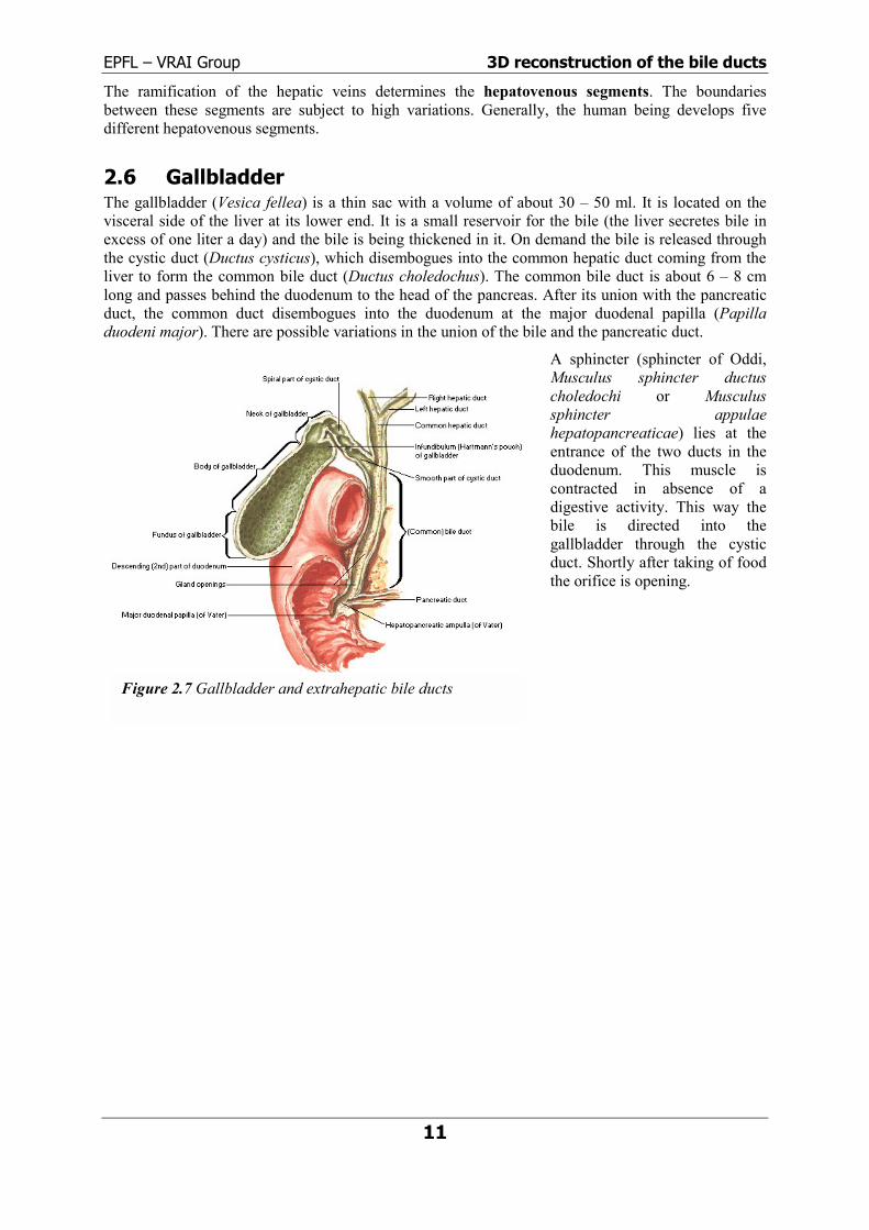
2.6 Gallbladder The gallbladder (Vesica fellea) is a thin sac with a volume of about 30 � 50 ml. It is located on the visceral side of the liver at its lower end. It is a small reservoir for the bile (the liver secretes bile in excess of one liter a day) and the bile is being thickened in it. On demand the bile is released through the cystic duct (Ductus cysticus), which disembogues into the common hepatic duct coming from the liver to form the common bile duct (Ductus choledochus). The common bile duct is about 6 � 8 cm long and passes behind the duodenum to the head of the pancreas. After its union with the pancreatic duct, the common duct disembogues into the duodenum at the major duodenal papilla (Papilla duodeni major). There are possible variations in the union of the bile and the pancreatic duct.
A sphincter (sphincter of Oddi, Musculus sphincter ductus choledochi or Musculus sphincter appulae hepatopancreaticae) lies at the entrance of the two ducts in the duodenum. This muscle is contracted in absence of a digestive activity. This way the bile is directed into the gallbladder through the cystic duct. Shortly after taking of food the orifice is opening.
Figure 2.7 Gallbladder and extrahepatic bile ducts

EPFL � VRAI Group 3D reconstruction of the bile ducts
12
3 Biomedical imaging
3.1 Medical imaging techniques
3.1.1 Magnetic Resonance Imaging (MRI) Magnetic Resonance Imaging (MRI) has become one of the most important imaging modalities since the 1980s. It is useful in many clinical situations. Its main advantages are:
• non-invasive, radiation is not ionizing
• excellent tissue contrast
• well adapted for soft tissue
• possible imaging of contrast medium
The technique is based on the alignment of the nuclear magnetic spin of protons (hydrogen atom) under the influence of an external magnetic field. This situation is disturbed by applying a radiofrequency (RF) pulse at a specific resonance frequency. The protons of the body absorb this energy. After the applied pulse has been stopped, the energy is given up and can be detected.
The measured signal depends on the hydrogen density and the relaxation time. Spatial information is obtained by employing magnetic gradient fields. This allows constructing a contrast image of the different locations (voxels). The different voxels are coded in frequency or phase shift and 2D cross-sections or even complete 3D images can be acquired.
3.1.2 Computed tomography (CT) Computed tomography is based on X-rays and allows acquiring cross-section images of the human body, which is not possible with normal X-ray projection images. To do so, a large set of X-ray projections is acquired by rotating the X-ray source around the patient. This provides projection images of the same scene from many different view angles. With image reconstruction methods the cross-sectional image can be established.
If many consecutive cross-sections are acquired, they can be piled up and connected to construct a fully 3D image like in the case of MRI.
The machines used for CT are so-called CT-scanners since they perform a complete scanning of the patient. The latest scanner generation includes helicoidal scanners, where the scanning is performed with a continuous translation at the same time. This allows a faster acquisition and therefore reduces the exposition of the patient to the harmful radiation, but complicates the reconstruction of cross-sections.
Figure 3.1 CT-scanner

EPFL � VRAI Group 3D reconstruction of the bile ducts
3.1.3 Angiography Angiography is a technique to represent vessels by injection of a contrast medium. Without any contrast medium the vessels would not be visible at all on the images. The acquired images are called angiograms. This technique is initially derived from X-ray imaging, which means that X-ray projections are taken after the injection of the contrast medium. However angiography is being applied with other imaging modalities as well, for instance magnetic resonance angiography (MRA) or computed tomography angiography (CTA). These techniques are based on the same principle with the injection of a contrast agent. With the initial X-ray technique the acquired image is a 2D projection. With CTA and especially MRA it is possible to directly visualize a 3D image of the vessel structure.
Digital Subtraction Angiography (DSA) Digital subtraction angiography is the application of the subtraction method with digitally stored images. Therefore two images of the same region are acquired: one image before the injection of the contrast medium and one image with the contrast medium. The only difference between these two images will be, that on the latter the vascular structures are visible but not on the former. By subtracting the two images the vessels will remain the only visible features on the resulting image. In section 11.4 this method will be illustrated based on real clinical data.
Acquisition systems As mentioned, angiograms are acquired by X-ray projection. From a mechanical point of view there exist three different possibilities for acquiring several angiograms with different angles to the object: biplane systems, rotational angiography and C-arms.
Biplane systems allow simultaneous acquisition of two projections with a different angle with respect to the object (generally 90°). This is widely used in cardioangiography for visualization of the coronary arteries. Rotational angiography allows a continuous rotation of the projection plane around the patient and thus a large number of projections are acquired while keeping the same reference for all projections. Both of these systems
inop
Apapran
Am19so
Figure 3.4 Principle of a biplane system
13
require some fix stallation, which most generally is not available in erating rooms.
C-arm is a mobile X-ray acquisition system and is rt of the standard equipment used in surgery. It ovides real-time feedback of anatomical structures d surgical tool positions.
t the end of the year 2000 Siemens presented a new obile C-arm, the SIREMOBIL Iso-C3D, which offers 0° orbital movement and dedicated hardware and ftware for 3D imaging. Its isocentric principle and the
Fig
Figure 3.2 A typical X-ray angiogram
ure 3.3 A mobile C-arm system

EPFL � VRAI Group 3D reconstruction of the bile ducts
14
motorized arm provide the basics for intra-operative 3D imaging. The product can be used either for conventional 2D imaging or in 3D imaging mode. This is the first mobile system providing a motorized acquisition system and an automatic 3D imaging mode to be used in operating rooms.
Cholangiography Cholangiography is the angiographic visualization of the bile ducts. There basically are three different methods to acquire cholangiographies, that is, to inject the contrast medium; two pre-operative methods (PTC and IVC) and one during operation (POC).
Intravenous cholangiography (IVC) is based on the fact that the liver is capable of eliminating certain substances immediately into the bile ducts. This makes it possible to perform a cholangiography by intravenous injection of a contrast agent. About 30 minutes later (depending on the chosen procedure) the contrast agent will have reached the bile ducts through the liver. The large hepatic ducts and the extrahepatic bile ducts will then be visible in a cholangiogram. However this technique has widely been abandoned due to its toxicity and occurring death cases.
Percutaneous transhepatic cholangiography (PTC) is performed by passing a needle through the skin, the ribs and the liver so that the contrast medium can be injected into the liver�s duct system. The needle is introduced until it has reached the level of the right border of the spine. This usually requires anesthesia of the patient and respiration has to be stopped during the insert of the needle. This procedure has to be executed with much care in order not to damage any part of an organ or the blood vessels. Most common complications are a leakage of the bile into the peritoneal cavity, intraperitoneal hemorrhage (bleeding) and septicemia (blood infection). Therefore this technique is only used, when it is absolutely necessary and no other possibility exists.
Per-operative cholangiography (POC) can be performed during an operation directly on the operating table during both open and laparoscopic operations. Generally a mobile X-ray acquisition system will be necessary in the operating room. The contrast medium is directly injected into the cystic duct with a syringe. There are very few complications with this method, including bile duct rupture and septicemia.
3.1.4 Ultrasound (US) Ultrasound is the only imaging technique that does not directly or indirectly involve electromagnetic radiation. It is a non-invasive technique that can also be used for therapeutic purpose.
Ultrasound waves are acoustical waves (pressure) above audible frequencies. There is a strong interaction between the intrinsic properties of the tissue (density, compressibility) and the wave propagation. With ultrasonic imaging, information about tissue properties can be determined by observing how waves are perturbed. The difficulty is to unravel the information into a useful image form.
Echography is a technique that uses the change of the acoustical impedance at interfaces between tissues to visualize the anatomical structures. At such an interface the sound waves are reflected and diffused. Generally the ultrasound is used in a pulsed mode. Measuring the amplitude and the time interval between emission and reception of the reflected echo allows to determine the biologic structure. The image is in 1, 2
Figure 3.5 Ultrasound probe for intraoperative diagnostic
Figure 3.6 Typical ultrasound image
EPFL � VRAI Group 3D reconstruction of the bile ducts
15
or 3 dimensions depending on the used mode.
The mode A (amplitude) is used to represent the echo depending on time, that is, on depth since the velocity of propagation may be assumed constant. This gives a one-dimensional representation.
B-scan imaging (B for brightness) is the recording of pulse echoes (echography) from a single transducer over time and space. This is a tomographic technique that produces cross-sectional slices perpendicular to the ultrasound probe. Hence it provides a two-dimensional image. Other artifices containing several transducers and producing rectangular images also exist.
Other modes like the TM (Time Motion) or D (Duplex) modes are extensions of the above. They are not considered here since they will not be used in any further considerations.
Ultrasound images are not very clear or accurate and often they are noisy. However this technique is very simple to use and quickly provides the surgeon with valuable information. It is a low cost system allowing real-time scanning, which is an important parameter.
3.1.5 Endoscopy Endoscopy is nowadays a widely used technique for operations. Especially laparoscopy (endoscopy applied in abdominal cavity) allows many operations to be much less traumatic for the patient. With endoscopy many operations can be executed in a minimal-invasive way. That is, the body must not be opened to access the area of interest for the operation. Only very few (3 to 4) and small incisions are made, which are just large enough to pass the endoscope and the operating instruments into the abdominal cavity.
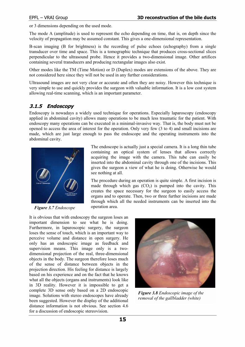
The endoscope is actually just a special camera. It is a long thin tube containing an optical system of lenses that allows correctly acquiring the image with the camera. This tube can easily be inserted into the abdominal cavity through one of the incisions. This gives the surgeon a view of what he is doing. Otherwise he would see nothing at all.
The procedure during an operation is quite simple. A first incision is made through which gas (CO2) is pumped into the cavity. This creates the space necessary for the surgeon to easily access the organs and to operate. Then, two or three further incisions are made through which all the needed instruments can be inserted into the operation area.
It is obvious that with endoscopy the surgeon loses an important dimension to see what he is doing. Furthermore, in laparoscopic surgery, the surgeon loses the sense of touch, which is an important way to perceive volume and distance in open surgery. He only has an endoscopic image as feedback and supervision means. This image only is a two-dimensional projection of the real, three-dimensional objects in the body. The surgeon therefore loses much of the sense of distance between objects in the projection direction. His feeling for distance is largely based on his experience and on the fact that he knows what all the objects (organs and instruments) look like in 3D reality. However it is impossible to get a complete 3D sense only based on a 2D endoscopic image. Solutions with stereo endoscopes have already been suggested. However the display of the additional distance information is not obvious. See section 4.6 for a discussion of endoscopic stereovision.
Figure 3.8 Endoscopic image of the removal of the gallbladder (white)
Figure 3.7 Endoscope

EPFL � VRAI Group 3D reconstruction of the bile ducts
3.2 Image analysis In this section an introductory description of some basic image analysis techniques is given. The knowledge of these techniques is necessary to understand the methods used and the ideas expressed in this work. However the reader should refer to dedicated books on the subjects for a profound understanding. [17] gives a very complete description of all levels of image reconstruction, from signal processing, image processing, transforms and filtering to the description of reconstruction techniques. [14] is more specific and gives a good survey on image processing. In [41] a complete state of the art of automatic image analysis in medical imaging is given, from segmentation, fusion and visualization to simulation and robotics.
3.2.1 Feature extraction There exists a vast amount of approaches and techniques to extract features in digital images. Only a short description of the different notions can be given here. For details refer to [14].
A first approach is edge detection. An edge is the outline of an object or, in other terms, the boundary between an object and the background. If edges are identified, the object is located and many of its characteristics are known too. Edges can be located by examining the difference in pixel values. Already very simple digital filters (gradient filters) allow detecting edges in well-contrasted images. This makes this technique so powerful and widely used.
Edwiinsanmethine
MobcoW(pdil
Skneofwhthaprco
3.Rebedif
ImHeheali
Figure 3.9 Edge detection16
ge detection is often part of a process called segmentation, which is the identification of regions thin images. However gray-level segmentation is often used on its own to detect an object. For tance, with a simple well-chosen threshold, an image can be divided into two regions: the object d the background. There exist statistic and iterative thods to find an optimal threshold. The assumption in s technique is that pixels with similar gray-levels in arby regions usually belong to the same object.
orphology considers the shape and structure of an ject to enhance the image. The idea is that pixels llect into groups to form a two-dimensional structure. ell-known basic morphological operations are erosion ixels matching a specific pattern are deleted) and atation (a small area is set to a given pattern).
eletonization is the attempt to extract the least cessary information to describe the structure or shape an object. Another term for this operation is thinning, ich means that only the pixels belonging to an object t are essential to communicate the object�s shape are
eserved. In the ideal case this provides a skeleton nsisting only of lines.
2.2 Registration gistration deals with the correspondence between two images of the same scene. These images can acquired with the same modality (that is, the same acquisition system) but also with completely ferent modalities. This makes registration an integral step in fusion of different imaging modalities.
ages acquired with different modalities in the clinical track of events usually are complementary. nce, an integration and fusion of this data into one image containing all useful information is very lpful for clinical use. Registration is the process that brings the different images into spatial gnment. Basically this consists of finding a transformation that brings one image in the correct
Figure 3.10 Segmentation with a binary threshold and corresponding histogram

EPFL � VRAI Group 3D reconstruction of the bile ducts
17
position with respect to the other image. This transformation naturally consists of a rotation and a translation in space, representing the 6 degrees of freedom, plus a possible scaling and/or deformation transformation. Transformations can be rigid, affine, projective or curved.
To find this transformation extrinsic markers placed in the images or intrinsic properties of the objects may be used. Gray-level matching criteria may for instance be used for intrinsic registration.
Registration is possible for two 2D or two 3D images, but there also exist methods for 2D/3D registration where the alignment of spatial data to projective data is resolved.
Maintz and Viergever [39] give a systematic and complete survey on the current state of the art of all registration possibilities and methods. This document is indispensable for everyone working with registration.
3.2.3 Epipolar geometry Epipolar geometry is the theory that describes the relation between two image acquisition systems (say two cameras) acquiring an image of the same scene or object from two different positions. To describe this situation, two aspects have to be considered:
1. Extrinsic parameters: the relative positions of the two cameras in three-dimensional space
2. Intrinsic parameters: the intrinsic characteristics and dimensions of the two cameras
Let us first define the model of a camera. When working with full perspective projection, the pinhole model is a reasonable approximation for the camera description. The light rays all pass through an ideal point C, which is the optical center or projection center. The object is then projected unto the image plane (BE) and turned by 180° with respect to the real object. For the sake of simplicity for further processing of the image data, the image plane is set to BE�, which does not change anything to the correct representation of the physical reality. The distance between BE� and C is the focal length f.
The different parameters and coordinate systems are defined as illuorigin of the 3D camera coordinate system (X,Y,Z) is placed at the ocoinciding with the optical axis of the camera. X and Y axes are disporder to coincide with the general pixel representation in digital imageimage coordinate system (x,y) has its origin at the intersection of the oin point c, called the principal point. The origin of the digital pixel coorthe upper left corner of the image such that the midpoint of the digiorigin of (x,y)
Figure 3.11 Camera pinhole model
strated in the next figure. The ptical center C with the Z axis osed as shown in the figure in processing. The continuous 2D ptical axis with the image plane dinate system (u,v) is shifted to tized image coincides with the

EPFL � VRAI Group 3D reconstruction of the bile ducts
18
.
Figure 3.12 Definition of the camera coordinate systems
The basic affirmation of epipolar geometry is that a point on one image is projected unto a line on the other image. This is easily seen by observing the next figure where M is a point in 3D space, and m and m� its projections unto the two images.
A point on an image actually represents the projection of an optical light ray through space unto the point on the image. That is, on that image this particular ray is only observed as a point. However if one looks at this same light ray from another direction, the ray will not only be seen as a point but as a line in space. This also is the case for the second camera that sees this light ray projected unto its two-dimensional image as a line, the so-called epipolar line.
In reverse, all points on this epipolar line are projected unto a line in the first image as well. This is the corresponding epipolar line. Hence, there always exist two corresponding epipolar lines on the two images.
Figure 3.13 Relative position of two image planes

EPFL � VRAI Group 3D reconstruction of the bile ducts
19
The line that connects the optical centers of the two cameras intersects with the image planes at two particular points, which are called the epipoles. All epipolar lines in one image pass through this point5.
Now the most basic equations of epipolar geometry that are used in this work will be established. For proves and detailed information please refer to [19] [u] [s].
Intrinsic parameters of the camera There are several intrinsic parameters, but only 5 degrees of freedom for the intrinsic matrix A of the camera:
���
�
�
���
�
�
⋅⋅⋅⋅
=���
�
�
���
�
� ⋅
100sin/0cot
100sin/0cot
=A cv
cuu
cv
cuu
vkfukfkf
vu
θθ
θαθαα
Where
f : focal length, in unit [m]
ku : unit along u with respect to units in (c, x, y), this is equal to 1 / PixelWidth
kv : unit along v with respect to units in (c, x, y), this is equal to 1 / PixelHeight
θ : angle between u and v axis, this can approximately be set to 90°
[u0, v0]T : coordinates of c in (o, u, v), in unit [pixel] this is equal to [NumberPixelsWidth / 2, NumberPixelsHeight / 2]T
Note: because the matrix depends on the products αu = f ku and αv = f kv, a change in the focal length f and a change in the pixel units ku, kv are indistinguishable!
The pixel width and height, which are the inverse of ku and kv, are determined as follows in the case of a CCD camera and a frame grabber:
lsWidthNumberPixesWidthureElementNumberPictmentWidthPictureEle
lsWidthNumberPixedthagePlaneWiImPixelWidth ⋅==
lsHeightNumberPixesHeightureElementNumberPictmentHeightPictureEle
lsHeightNumberPixeightagePlaneHeImtPixelHeigh ⋅==
Where
PixelElementWidth width of a single picture element on the sensing chip of the camera, in unit [m]
NumberPictureElementsWidth number of picture elements in the width on the sensing chip of the camera
NumberPixelsWidth number of pixels grabbed in the width
PixelElementHeight height of a single picture element on the sensing chip of the camera, in unit [m]
NumberPictureElementsHeight number of picture elements in the height on the sensing chip of the camera
NumberPixelsHeight number of pixels grabbed in the height 5 In stereovision where the two image planes generally are parallel, the epipoles lie in infinity and all epipolar lines are horizontal and parallel.

EPFL � VRAI Group 3D reconstruction of the bile ducts
20
Note: in the case of continuous acquisition systems like X-rays for example, there are no picture elements and the width and height of the image plane must directly be given.
The intrinsic matrix A describes the projection of a point in space unto the image plane and the conversion into pixel image coordinates:
����
�
�
����
�
�
⋅���
�
�
���
�
� ⋅=
����
�
�
����
�
�
⋅=���
�
�
���
�
�
11000
11Z
YZ
X
vsin/ucot
ZY
ZX
Avu
cv
cuu
θαθαα
mAvu
AZY
ZX
x ~
11
~ 11 ⋅=���
�
�
���
�
�
⋅=
����
�
�
����
�
�
= −−
Extrinsic parameters The extrinsic parameters describe the relative position between two cameras. That is, one camera is brought to its position by rotation and translation from the position of the other camera. Obviously there are 6 degrees of freedom for such a transformation in 3D space.
A rotation matrix R and a translation vector t describe this transformation. For the rotation matrix, a rotation with angle θ around the y-axis is given as an example.
���
�
�
���
�
�
−=
θθ
θθ
cos0sin010
sin0cosR
���
�
�
���
�
�
=
Z
Y
X
ttt
t
Now a space point [X,Y,Z]T in the first camera coordinate system has coordinates [X�,Y�,Z�]T in the second camera coordinate system:
���
�
�
���
�
�
+���
�
�
���
�
�
⋅���
�
�
���
�
�
−=+
���
�
�
���
�
�
⋅=���
�
�
���
�
�
Z
Y
X
ttt
'Z'Y'X
cossin
sincost
'Z'Y'X
RZYX
θθ
θθ
0010
0
The essential matrix E describes this transformation in a compact way and is defined as follows:
[ ] Rtt
tttt
RtE
XY
XZ
YZ
⋅���
�
�
���
�
�
−−
−== ×
00
0
Which leads to the epipolar equation:
0'~~ =⋅⋅ xEx T
Where x~ and '~x are the two images of the same space point [X,Y,Z]T.
Fundamental matrix The basic epipolar constraint that a point on one image must be on a line in the other image is expressed like this: if two points m and m�, expressed in pixel image coordinates in the first and second camera, are in correspondence, they must satisfy the following equation:
0'~~ =⋅⋅ mFmT
Where F is a 3 × 3 matrix, the so-called fundamental matrix: 1'−− ⋅⋅= AEAF T
There are 7 degrees of freedom for this matrix. All that needs to be determined are the intrinsic matrix A and the essential matrix E, and the epipolar lines can then easily be computed. If the coordinates of

EPFL � VRAI Group 3D reconstruction of the bile ducts
a point in one image are introduced in above equation, this directly yields the equation of a line in the other image, the epipolar line.
3.2.4 Reconstruction Reconstruction appeared with the first CT-scanners (computed tomography) were the images have to be reconstructed from projections. In the case of CT a high number of projections is acquired to provide enough information for a safe reconstruction. This is where conventional reconstruction methods have their origin.
Later, applications appeared where it was not possible to acquire enough projection images to provide all the necessary information for reconstruction. These so-called ill-posed reconstruction problems needed adaptations of the conventional algorithms and the development of new algorithms.
Reconstruction methods generally belong to one of two categories:
• Analytical approaches (or convolutional backprojection techniques): These methods are based on the inversion of the projection operator. The Radon transform, which describes the projection images in function of the view angle, plays an important role in these methods. All the projections can then be projected back (backprojection) to construct the image. However the reconstructed image will appear smoothed. To avoid this effect, a method called filtered backprojection (FBP), which incorporates a high-pass filter into the reconstruction algorithm, has been introduced.
• Algebraic approaches: Algebraic reconstruction techniques (ART) are based on the minimization of the reprojection error using an iterative scheme. This approach is conceptually simpler. There exists a large amount of variations of the basic ART, like SIRT (Simultaneous iterative reconstruction technique), SART (Simultaneous algebraic reconstruction technique), SRT (Segmental reconstruction technique), MART (Multiplicative algebraic reconstruction technique) and ICM (Iterated conditional mode).
An important detail lies in the nature of the radiation used. Different reconstruction algorithms are used depending on whether the cone-beam problem has to be solved or whether parallel rays are used. In the case of parallel rays and a large number of projection views, it would typically be the Radon
transform and an analytical algorithm that would be used for reconstruction.
To solve under-determined or ill-posed reconstruction problems, several �standard� solutions are known. However this is still a domain of research. Generally algebraic reconstruction algorithms are preferred to analytical ones, since only a small number of views can be acquired and the X-ray source trajectory covers only a limited angle. Additional constraints (a priori knowledge) have to be introduced to solve ill-posed problems. Methods
toprpo
Figure 3.14 Parallel and cone-beam irradiation
21
include a priori knowledge in reconstruction algorithms are regularization, maximizing a priori obability (Maximum a posteriori MAP estimation, Bayesian estimation, Markov random fields) or sitivity and compact support.

EPFL � VRAI Group 3D reconstruction of the bile ducts
22
4 Fusion possibilities
4.1 Survey For abdominal surgery, there are several imaging techniques to take into consideration. These techniques as well as the possibilities to fuse images acquired with the different modalities will be outlined here. The focus is on possible exploitation for hepatic and pancreatic surgery. Hence, the visualization of the bile and pancreatic ducts is an important issue.
Abdominal surgery is executed minimal-invasively, using an endoscope for general visualization of the structures and organs, which are not directly visible anymore. This kind of surgery is called laparoscopy (abdominal endoscopy). Note that the direct three-dimensional vision of the scene is lost and only a 2D projection on a screen is available. Other widely used techniques, such as MRI (Magnetic Resonance Imaging) and ultrasound (US) echography are applied in the same context.
To visualize organs and their vessels in the abdominal area (liver, gallbladder, pancreas), one can make use of a special technique. The used imaging technique is called angiography (cholangiography in the case of the bile ducts). For this technique a contrast medium is injected into the vessels, and then images are acquired by X-ray projection.
Conventional pre-operative CT-scans (computer tomography) will not be very useful, since the bile ducts are not visible without a contrast medium. A contrast medium for the bile ducts can only be given in an invasive way before the operation. However it is possible to perform CT-scans during the operation but this implies the possibility of having a complete CT installation in the operating room. The possibility of CT-scans is therefore not considered in this section. Note however that the use of dedicated CT installations in the operating room may become possible in the future. This could obviously simplify the acquisition of images of certain structures, but acquisition time is sure to be higher than with simple X-ray projections.
MRI may be used in two or three dimensions. Currently the surgeon uses several 2D slices taken before the operation for pre-operative planning. For computer assisted surgery a 3D reconstruction becomes particularly interesting. In this case a three-dimensional model of the examined structure can be constructed by using several consecutive two-dimensional slices. This 3D-model can later be used for fusion with other images in order to provide a better and more complete image of the anatomical structures. The model is acquired and constructed once before the operation. It is then used throughout the operation and any fusion process without any additional acquisition. This limits the available possibilities to correctly adapt the model in the track of a surgical intervention.
Per-operative ultrasound probes provide two-dimensional slices corresponding to cross-sections of an organ. Note that these probes are entirely manipulated by the surgeon and the surgeon himself is not aware of the exact orientation and position of the probe. The quality and type of the acquired images is therefore much dependent on the manipulator and may be different for every surgeon.
All of these techniques, MRI, US, endoscopy and angiography, may be used for fusion. When merging image data of different imaging modalities, two important issues have to be addressed:
1. Resolution of each imaging technique
2. Acquisition time in the case of real-time applications

EPFL � VRAI Group 3D reconstruction of the bile ducts
23
In the following sections each possible fusion between two modalities will shortly be explained. Below you see a quick survey to jump to the corresponding section.
Fusion MRI Endoscopy Ultrasound Angiography MRI 3D-model § 4.2 § 4.3 § 4.5.3 Endoscopy § 4.6 § 4.4 § 4.5.2 Ultrasound § 4.5.4 Angiography § 4.5.1
Table 4.1 Fusion possibilities and corresponding sections
4.2 MRI � Endoscope fusion This type of fusion consists of correctly placing a 3D-model (constructed by MRI) of an anatomical structure in the endoscopic image. This allows localizing structures that would not be visible otherwise, directly in the endoscopic image. This is also referred to as �X-ray vision� since one can sort of �see through� the organ (which also is possible with X-ray images, hence the name although there are definitely no physical X-rays involved here). To perform registration, a 3D reference frame has to be placed in the endoscopic image. This way, the position of the camera with respect to this frame is known at every moment. The surgeon may now localize at least three visible points in the image corresponding to well-defined points in the 3D-model. Of course the points in the image must be localized in a three-dimensional space. This is possible due to the use of the reference frame in the endoscopic image.
4.3 MRI � Ultrasound fusion For this fusion the MRI 3D-model is used as well. This time the task is to localize the ultrasound probe with respect to the model. This will allow the surgeon to see the ultrasonic cross-section correctly placed in the three-dimensional model of the anatomical structure.
Figure 4.2 Ultrasound cross-section in 3D MRI model
4.4 Ultrasound � Endoscope fusion This type of fusion is similar to the fusion of MRI and ultrasound (section 4.3), only that there is no 3D-model this time, but �only� a two-dimensional endoscopic image. The endoscope also is in motion
Figure 4.1 Endoscopic image with superimposed MRI 3D-model

EPFL � VRAI Group 3D reconstruction of the bile ducts
24
and manipulated by the surgeon at the same time as the ultrasound probe. The idea is to display the ultrasound cross-section in the endoscopic image.
Of course, endoscope and ultrasound probe may be aligned at some moment such that only a 1D projection (a line) of the 2D ultrasound cross-section will be visible in the endoscopic image, which obviously will not add any additional information to the image. For this case the ultrasound cross-section could be displayed in one corner of the image without any matching procedure performed. On the other hand, it is possible to track the ultrasound probe with a tracking system in order to know the position and orientation. This information could be used to indicate to the manipulator if the probe is acquiring useful images in its current position.
4.5 Angiography
4.5.1 Angiography 3D reconstruction One single angiography provides a two-dimensional projection of some aHowever it is possible to reconstruct a three-dimensional model with a mA priori knowledge of the observed structure can drastically reducprojections. In the case of vessels or ducts a simple model consists of jucones) and bifurcations. With this model two or three projections fromsufficient. With a conventional C-arm that is used for angiography,projection is known and can directly be used for reconstruction, sincbetween two consecutive acquisitions.
To reconstruct a 3D-model from two projections, these images have to be calibrated first in order to assign them to ideal images. Distortion is produced by the optical system as well as the physical acquisition process. Only the ideal, calibrated images are used for reconstruction. In order to match the two images, unique anatomical structures such as bifurcations have to be detected. From these points the correspondence between the two images can be found, and the 3D-model can be constructed.
Practically between 2 and about 10 projections from different angles will be necessary to fully reconstruct the vessel or duct system. The number of necessary projections depends on the desired accuracy of the local shape of the vessels. A technique called DSA (Digital Subtraction Angiography) may be very helpful for segmentation of the vessels. But to use this technique, two angiograms from each angle are necessary, one angiogram without contrast medium and one following these two images can be subtracted and only the vessels wiimage. This procedure doubles the number of necessary acquisitions, acquisition, for the change of the angular position of the C-arm and medium also need to be taken into consideration. Since the patient macquisitions necessary for one DSA, and the translational position (x,y,angular position may be slightly different, a registration of the two image
4.5.2 Angiography � Endoscope fusion The fusion of the constructed model with the endoscopic image is similarthe MRI-Endoscope fusion (section 4.2, see also figure there). But thiscan already be placed before acquiring the angiograms. The reference both, the angiogram and the endoscopic image. This may help to m
Figure 4.3 Ultrasound cross-section in endoscopic image
natomical structure (vessels). inimal number of projections. e the number of necessary st two elements: cylinders (or different directions may be
the angular position of the e the patient will not move
with contrast medium. In the ll be visible on the resulting and the time constraints for for the flow of the contrast ight move between the two
z) of the C-arm as well as its s will become necessary.
to the principle explained for time the 3D reference frame frame will then be visible in ore directly register the two
Figure 4.4 Example of a reconstructed 3D vessel network

EPFL � VRAI Group 3D reconstruction of the bile ducts
25
images. Some surgical tools that are used anyway during the operation will be visible in the images and can even be used as reference frame.
The fusion of a single 2D angiogram projection and the endoscope is another possibility. However this only makes sense when the endoscope �looks� in the same direction, in which the angiographic projection has been taken. Otherwise there will be no well-defined position to put the angiogram in the endoscopic image.
4.5.3 MRI � Angiography fusion This type of fusion consists of finding the correspondence between two 3D-models. On the one hand the MRI provides a model of the organ, whereas the angiography provides a model of the vessels or ducts of that organ. This allows displaying one single 3D-model containing complete information about the organ, which is not the case for either of the two models alone. This problem falls back on a 3D/3D registration (see § 3.2.2). An example of this fusion is given in [49].
Here as well it is possible to fuse a single 2D angiogram projection and an MRI 3D-model. In this case, the task would be to correctly superimpose the 3D-model on the 2D projection. It is obvious that there only is one single solution to put the 3D-model on the projection. For an additional visualization in 3D space (rotation of the 3D model) the angiographic projection would have to be displayed in perspective below the model, since the latter cannot be superimposed on the projection anymore. In this case the problem falls back on a 2D/3D registration. Here a 2D projection is registered to a 3D model, which should not be confused with registering a 2D cross-section with a 3D structure as mentioned in section 4.3. The advantage of the use of a single projection is that much less time is necessary for acquisition and processing than for reconstructing a complete 3D-model with several angiographies. An example of such a fusion is given in [70].
In the following figures, a reconstructed carotid artery can be seen on the left, and the fusion of the two 3D-models is represented on the right (only one cross-section displayed). The same fusion principle as for cerebral surgery may also be applied to abdominal organs.
Figure 4.5 3D reconstruction from angiograms Figure 4.6 Fusion of angiography and MRI
4.5.4 Ultrasound-Angiography fusion The fusion of angiography and ultrasound echography is a possibility that is useful to assess coronary artery diseases. The first provides a projection of the vessels containing information about topology and shape. The second offers the possibility to acquire cross-sections of the vessel, which allows gathering information about the vessel wall. Obviously there is no geometric relationship between consecutive cross-sections acquired with ultrasound. The relatively new intravenous ultrasound (IVUS) is used to acquire cross-sectional images of the coronary vessels.
Hence, there is a necessity to fuse in three-dimensional space the 2D angiographic projection with the sequence of ultrasonic 2D slices. This combination will allow seeing in one image the longitudinal and cross-sectional geometry of coronary arteries. An example of such a fusion can be found in [71].

EPFL � VRAI Group 3D reconstruction of the bile ducts
26
4.6 Endoscopic stereovision In endoscopy the use of two cameras is possible. This provides additional information about the distance to objects. However this generally is not very precise and the display of this information is not obvious. One option is to make the surgeons wear special glasses, which will automatically provide the left eye with the left image and the right eye with the right image. This gives the surgeon a three-dimensional impression of the scene. Another possibility is to display the distance information with gray-levels (or different levels of any other color). High intensity would correspond to close objects, low intensity to far objects.
Additional devices that the surgeon has to wear do not increase his comfort. There exist image overlay systems where medical images may be displayed on the patient during surgery ([39]). In these systems, a transparent displaying screen is placed between the surgeon and the operating scene. Such a system might also be used to display depth information. But still, this will probably never be totally equal to a real three-dimensional perception of the scene in terms of quality and comfort.
The main issues remain:
1. Resolution
2. How to render the depth information
In the example of opposite figure, three additional indications are represented with different colors:
• The colored indicator on the instrument represents the distance of the instrument to the organ on a straight line.
• The colored area on the organ represents the distance of the instrument to the corresponding section on the organ. For both red is close and violet is far.
• The two green arrows represent the distance of the instrument to the target marked with an X.
4.7 Discussion The preceding sections show that there is a large number of possibilities to merge information into a single image to help the surgeon plan and perform operations. Some fusions pose similar problems, for others completely different issues have to be addressed.
Ultrasound still is a particularly difficult modality to fuse with other modalities. This has several reasons. First their use much depends on the manipulator (the surgeon). It is impossible to have a reliable a priori indication about the location and position of the probe. Second, the image quality is not very good and images may have several artifacts. Research on ultrasound fusion may have begun (see [71]), but is still in an initial stage.
The fusion of a three-dimensional model with endoscopic images as explained in section 4.2, is a problem that is already managed by 2C3D SA. Endoscopic stereovision also is an issue that is mastered in terms of acquisition and computation, but an adapted system for representation of the information in clinical use does not exist yet.
On the other hand, the information provided by angiographic images and their representation in three-dimensional space seems to be an interesting problem. First the reconstruction problem has already been studied for several years and seems to be solvable with reasonable efforts, the current acquisition equipment and computation power available. And second, the angiographic imaging techniques that are used in clinical routine for visualization of the bile and pancreatic ducts could be valorized. The next chapter gives a detailed introduction to the problem of reconstructing a 3D model from angiographic projection images.
Figure 4.7 Additional distance information in stereovision

EPFL � VRAI Group 3D reconstruction of the bile ducts
5 3D reconstruction from angiographic projections
5.1 Problem statement
5.1.1 Introduction The present work will focus on the fusion of a 3D model of the bile ducts with endoscopic images. This will allow to �see through� the liver and to locate the bile ducts directly on the endoscope. In a final step it should be possible to automatically determine the different liver segments based on the distribution of the bile ducts (see § 2.5.2). The 3D model is reconstructed from angiographic X-ray projection images, which is the main part of the presented work.
After a short introduction and the specification of the requirements for the system, the current state-of-the-art is presented. It follows a short description of the proposed solution and the acquisition procedure and finally a more detailed description of all the necessary procedures to perform a 3D reconstruction.
Applications Such a fusion is useful for several operations concerning the liver as well as the pancreas, since the pancreatic duct is connected to the common bile duct. Possible applications are partial hepatectomy (excision of a part of the liver) in the case of cancer, metastasis and malformation or for liver donors (transplantation). Another application is the treatment of echinococcosis, a disease caused by an infestation of tapeworms upon ingestion of eggs. In 60% of the cases this incites the illness of the liver. The chronic pancreatitis, mostly caused by chronic alcohol consumption, and the possible formation of a pseudocyst will require the partial resection of the head of the pancreas. This and other surgical interventions in the pancreas are further applications for this fusion.
Liver transplantation merits particular attention. Liver tissue is able to rebuild missing neighboring tissue. Hence, patients who need their liver to be replaced, may also be implanted only half a liver. If the liver of a donor could correctly be divided into two parts by carefully observing the detected liver segments, a single liver could serve as a substitute organ for at least 2 patients. This would considerably increase the available livers for transplantation. Note however that not all livers can be split. Currently only the livers in best conditions are considered for splitting.
A 3D model of the bile ducts In all applications the surgeon needs to resect a part of either the liver or the pancreas. To do so, not only the surface and the tissue of the organs has to be considered, but also the vessels and ducts that supply the organs with blood and conduct the bile and the pancreatic juice to the intestine. In the case of the liver, three systems (arterial, portal vein and bile ducts forming the liver triad, see § 2.5.2 for details) are supposed to have about the same distribution of vessels in the organ. This distribution defines different liver segments that can be resected.
Currently these vessels are localized with per-operative ultrasound (§ 3.1.4), which does not allow an accurate and completely reliable determination of the segments. All these operations would best be executed by laparoscopy in a minimal invasive way in order to keep the patient�s stress as low as possible. Hence, it would be very useful to have a 3D model of the vessels superimposed on the endoscopic image, which is at the same time the
Figure 5.1 Two angiograms of the same scene from different view angles
27

EPFL � VRAI Group 3D reconstruction of the bile ducts
28
only remaining perception for the surgeon. This would allow determining in real-time the location of a specific liver segment on one single image at every moment of the operation.
Before fusion, the 3D model of the bile ducts has to be constructed from projection images. Therefore cholangiographies of the duct system have to be acquired from different view angles. As seen in § 3.1.3, it is preferable to perform cholangiography intra-operatively. Hence, image acquisition as well as the reconstruction of the 3D model has to be performed during the operation. This requires respecting certain clinical time constraints.
Nowadays, per-operative cholangiography is a routine procedure in clinical use to visualize the bile ducts. During the operation the surgeon can access the bile ducts in a simple and atraumatic manner. Since the branches of the arterial and portal systems follow the intrahepatic bile ducts, this method is perfectly suited for a 3D reconstruction of the intrahepatic system and a following superimposition on the endoscopic image.
Visualization of vessels Obviously, the visualization of the portal vein or the hepatic artery would provide similar information to reconstruct a 3D model for fusion. Two cases have to be distinguished, the per-operative and the pre-operative image acquisition.
In the case of per-operative visualization the puncture of vessels to inject a contrast dye is a very risky procedure that has to be avoided:
• Arterial puncture may lead to a total dissection of the artery, which may in turn lead to the loss of the organ. The injury of the artery may have persistent leakage as consequence with formation of a pseudoaneurysm, which may cause death.
• Puncture of the portal vein entails the risk of lesion of the portal, arterial and bile duct system.
• The contrast agent for intravascular angiography is toxic and may produce allergies.
Furthermore, special acquisition systems are necessary for arterial angiography due to the blood flow. Hence, arterial or venous angiography is not performed during routine interventions.
It is possible to acquire pre-operative images of arteries or veins. This can be done by using an X-ray CT-scanner. Therefore a contrast medium is injected intravenously and several seconds later it reaches the organ in question. The time taken by the contrast medium to get from the injection location to the organ has to be known exactly by the radiologist in order to start scanning at the right moment.
The following list aims to give a short comparison between the pre-operative visualization of vessels and the proposed per-operative visualization of the bile ducts.
• Per-operative visualization of the bile ducts would give the surgeon an additional easy-to-use tool that directly considers the real situation during the operation. The reconstructed model will best correspond to reality. The acquisition procedure is based on routine techniques used on a daily basis.
• For per-operative cholangiography a reference frame can directly be placed in all images involved. This considerably simplifies the fusion of the model with real-time endoscopic images.
• The injection of a contrast agent into the bile ducts is not toxic.
• For pre-operative vessel visualization the reconstruction of a 3D tree-like structure from several CT-slices becomes necessary, which is not an obvious task.
• Due to the blood flow the image acquisition of vessels is more difficult than per-operative cholangiography. In the latter case the contrast medium slowly propagates into the different ducts.
• The two procedures can be complementary; vessel visualization for pre-operative planning and duct visualization for per-operative guidance.

EPFL � VRAI Group 3D reconstruction of the bile ducts
29
• Pre-operative MRI might offer new possibilities in the future since the vessels can be visible without injection of a contrast agent.
5.1.2 Functional specifications The constraints for such a 3D reconstruction system are mainly determined by the fact that it has to entirely run in the operating room. This implies several choices and constraints:
• For the reasons exposed in the introductory section, the cholangiography is used as imaging technique for visualization of the bile duct system.
• In the operating room, no fix installation will be available for any imaging system. Hence a mobile C-arm is used as X-ray acquisition system. Some additional registration or calibration will be necessary since the system is mobile.
• During an operation the time for the whole necessary acquisition should not exceed 5 minutes.
• This implies the constraint to reduce the number of angiographic projections to a strict minimum.
• In order to take all the projection images of the same scene, the patient�s respiration has to be stopped during the acquisition process. This is possible during 1 � 3 minutes several times.
• A minimal number of 3 bifurcation levels of the bile ducts need to be visible in the reconstructed model in order to allow a unique determination of the liver segments.
• The time for computation should not exceed 5 minutes.
• The superimposition of the reconstructed 3D model on the endoscopic image has to be performed in real-time. The 3D model will be rigid in a first phase.
• The 3D reconstruction obviously has to be performed automatically. However for the extraction of the ducts from the raw images and to find some initial point correspondences a manual initialization may be considered if it simplifies the whole procedure in terms of error rate and time requirements.
• The determination of the duct diameters does not have to be accurate since the goal is to visualize the structure and locations of the different segments rather than the exact shape of the ducts.
• Generally, accuracy on a small scale is not an issue. The aim is to correctly reconstruct the topology of the duct structure with an approximate metric indication of the order of ±5 mm.
• The two preceding points might have to be modified for the use of the system in applications where the small lesions of the bile duct system have to be identified.
In short, the aim is to develop a system to reconstruct a three-dimensional model of the bile ducts from very few projection images acquired with a simple-to-use system in as less time as possible.
5.2 State of the art The problem of reconstructing the bile ducts� structure from few angiographic projections is extremely ill-posed. That is, the few images available provide much too less information to correctly and uniquely reconstruct the three-dimensional structure. The image input data may also be incomplete and several solutions of the reconstruction problem may exist.
Additional information about the bile ducts is needed in order to allow a reconstruction at all and to eliminate wrong solutions of the problem. This information is provided in the form of so-called a priori knowledge, which may be anatomical and physiological properties of the bile ducts or knowledge about their topology. For instance, the most obvious a priori knowledge is, that the ducts resemble a cylinder and may approximately be described by its model. A summary of possible a priori knowledge for the reconstruction of the bile ducts is given in section 5.6.

EPFL � VRAI Group 3D reconstruction of the bile ducts
30
The reader is reminded of the difference between a 3D image and a 3D model. A 3D image is composed of voxels or volume elements, which are little cubes that are assigned a gray-level or color value. In a 3D model each point is associated to some well-defined structure, and all elements of an object are topologically connected. Thus, a model is a higher-level representation of an object than an image. This representation is much closer to human perception. We do not perceive objects in terms of pixels or voxels, but in terms of structure, shape and features.
In the following paragraphs, the most important articles in the field of ill-posed reconstruction problems and particularly of the reconstruction from angiographic projections are presented in summarized form.
An often-used system in recent research projects is the biplane X-ray acquisition system (see § 3.1.3). Further many researchers focus on the 3D reconstruction of the coronary artery tree, which is somewhat simpler than the reconstruction of the bile ducts. The coronary artery supplies the myocardium (cardiac muscle) with blood.
Fessler and Macovski [55] implemented a 3D reconstruction of arterial trees from 4 noisy projections acquired with the MRSIR technique for magnetic resonance angiography (MRA). To translate the reconstruction into an object estimation problem, they describe an extension of the generalized-cylinder object model that exploits the a priori knowledge about artery structures. Their method is applied to simulated projection images, a phantom and to real carotid angiograms. The system requires some manual initialization and takes half a minute to some minutes for execution.
Nguyen and Sklansky [54] present several ideas on the reconstruction of the 3D medial axes of coronary arteries. They use the motion of the heart and of the coronary arteries during cardiac cycles to estimate depth coordinates with the steepest descent algorithm. The motion is made visible by cineangiograms from a single view, that is, a sequence of angiograms. Typically 15 artery branches would be visible. In this precise work, the skeleton of the arterial tree is identified manually on each image. The next step is to find correspondences in successive images and then to estimate the 3D structure.
Sullivan et al [53] propose a hybrid method using both geometric and intensity information to reconstruct multiple curved objects. Four or five 1D X-ray projection images of the same object from different views serve as input. The algorithm then reconstructs the boundary of the object in 2 dimensions and provides a low-degree spline curve representing the object boundaries. Thus, it does not provide material density values, but the object borders. The process of feature grouping (subsets associated with different object boundaries) is executed manually. Execution time is about half an hour with 10 iterations.
The goal of the work of Launay et al [49] [50] is to detect arteriovenous malformations (AVMs) in 3D images. They present adapted algorithms using conventional iterative 3D reconstruction methods such as ART, MART, but also a new algorithm, DSI (discrete smooth interpolation). They use biplane DSA systems under stereotactic conditions and acquire 6 projection images of the carotid arteries, one projection every 30°. The most critical factor is image quality in projections and small caliber arteries are not visible. A fusion with other imaging modalities such as MRI is also presented.
The work and thesis of Payot et al [20] [51] [52] focus on the precise reconstruction of 3D images using iterative algorithms, which are well adapted for a large number of projection images (ART, SIRT, ICM). About 40 projections over 180° acquired in 2 seconds are needed. A Bayesian approach in association with Markov Random Fields is used to incorporate a priori knowledge. A stabilizing energy is used to smooth the 3D image and local curvature estimation enhances the contrast of small vessels.
Koppe and Kemkers et al [45] [46] have studied the use of rotational angiography for 3D reconstruction. This system basically consists of a motorized C-arm. They also explain the whole calibration and acquisition procedure. First they used 15 to 20 selected projections for reconstruction, which is performed with a cone-beam algorithm proposed by Feldkamp. In the second paper 100 contrast filled images acquired on a range of 180° are used (6 seconds for acquisition). Reconstruction itself takes about 10 minutes.

EPFL � VRAI Group 3D reconstruction of the bile ducts
31
Krissian et al [43] [44] extend a method to segment and reconstruct vessels in 3D images by using a multiscale detection algorithm. The focus is on complex 3D vessel networks and the detection of aneurysms. The 3D images are produced with the reconstruction method proposed by Payot [20]. In addition a cylindrical vessel model is used to produce good parameters. Execution time is about 7 minutes while some stages still are performed manually.
Soler et al [47] describe an automatic segmentation of 3D images. The method is applied to the structure of the portal vein. The procedure consists of filtering, application of thresholds and the final incorporation of a priori knowledge. The topological and geometrical constraints introduced by a priori knowledge basically correct the errors created during the previous segmentation steps. The result is an extracted model of the portal vein to be used later for the automatic determination of the anatomic liver segments.
Chen and Carroll [56] present a method to accurately reconstruct the 3D model of the coronary arterial tree from two angiographic projections. The 3D model is used to determine the optimal view angle for further diagnostic and therapeutic procedures. This is possible since the model may be rotated freely in space to find the desired optimal view angle. They describe the reconstruction process in 3 steps: 1. Recognition of 2D coronary arteries in both projection images and identification of bifurcation points, 2. Determination of the spatial relationship of two views, 3. Solving the correspondences of image points on the two images by epipolar constraints and calculation of 3D vessel centerlines knowing the transformation that defines the two views.
Dumay [21] examines the 3D reconstruction of the left coronary arterial tree from biplane angiographic projections. He applies a tracking approach for the segmentation and extraction of the vessel contours (see section 7.2 for details). The extracted tree is then labeled according to a graph representation of a geometric model (or simply a topological model) of the coronary tree and the segments are identified in both projection images. This allows finding the correspondences. Knowing the projection geometry, a set of 3D points can then be reconstructed. The correspondence between points on matched segments is found with a simple linear transform. However this solution needs improvement according to the author. Segmental reconstruction technique (SRT) and Network programming reconstruction technique (NPRT) are introduced to incorporate a priori knowledge into the reconstruction.
Cronemeyer [18] describes a detailed investigation on the 3D reconstruction of the coronary tree from biplane angiograms. Three different methods for the feature extraction are presented and compared. Bifurcation and terminal points of the coronary tree are determined and used to establish a global cost function for the correspondence between the two images. This cost function is minimized with a two-dimensional Hopfield neural network with several adaptations. An additional surface model is used as a priori knowledge; the coronary arteries all lie on the myocardium, and thus, on the heart�s surface. The reconstruction algorithms are tested on phantom models only. The execution time is between several seconds and 15 minutes depending on the used methods and hardware systems.
5.3 Proposed solution The approach in this work is somewhat different from most of the presented works. While many researchers focus on the accurate reconstruction of voxel based 3D images, the aim here, is to reconstruct a topological model of the 3D structure, as described by Chen and Carroll [56], Dumay [21] and Cronemeyer [18]. The reconstruction is performed based on two projection images.
As will be seen later the main problem of such a 3D reconstruction is to find the correct corresponding points in all projection images. This is necessary to find a unique reconstruction. In the case of projection images of vessels or ducts the principal error sources to this matching are the following:
• covered vessels, segments hidden behind other segments in one or both images
• vessels terminating into other vessels, this can lead to the detection of an actually non-existent bifurcation and to the creation of loops
• apparent intersections of vessels in 2D

EPFL � VRAI Group 3D reconstruction of the bile ducts
• hidden bifurcations, which will make the bifurcation appear at different locations in different images
Of course, all these problems may appear in combined form on one or both images, which considerably limits the chances to find a correct solution to the reconstruction problem. A further problem is the computation of the segment width or diameter in the case where this segment overlaps itself.
In the case of the bile ducts it is not possible to use a surface model for the duct distribution since they can be freely distributed in space unlike coronary arteries, nor is it possible to use an a priori topological model since the structure may vary on different levels between patients. The possibility to use a sort of pseudo-atlas by acquiring a pre-operative CT-scan for each patient must be avoided for reasons explained earlier, namely that a pre-operative injection of a contrast dye generally is not advised.
In order to better solve the problems mentioned and to be able to distinguish between several possible correspondences in static images the following solution is proposed:
Several images are acquired during the injection of the contrast medium. This allows seeing the propagation of the contrast flow in vessels, which will give valuable information about the vessels and their arrangement. The contrast medium generally propagates with a velocity of 5 to 20 mm/s. The entire duct
coprOtamviclsusa
T
6 l
Figure 5.2 Problems for reconstruction. Case I: no problem, all segments are present. Case II: hidden segment in one image. Case III: hidden segments in both images. Case IV: intersection and loop.
32
system is filled with the ntrast medium within 15 � 30 seconds. The pressure applied by the surgeon can control the opagation, however the control is strongly limited due the high mechanic resistance of the catheter. nce the contrast agent has fully filled the vessels a final image from another view angle at 90° is ken. Images with an angle of 90° in-between provide a maximum of 3D information and moreover a aximal accuracy of the depth information. It is possible to additionally acquire images from other ews to solve possible ambiguities. However this must be within the time constraints imposed by the inical circumstances6. For the dynamic images of the flux it is possible to directly apply the btraction method (DSA, § 3.1.3) since the camera position with respect to the object will remain the me for all images. This allows a simpler extraction of the duct�s contours and centerlines.
he flux information is useful in the following situations:
• Intersections of different ducts: flux arrives at the intersection at different moments. This allows distinguishing the two situations illustrated in the figures below.
Figure 5.3 Two intersecting segments Figure 5.4 Two touching segments
ess than 1 � 3 minutes, which is the time during which the patient�s respiration can be stopped

EPFL � VRAI Group 3D reconstruction of the bile ducts
33
• Intersections: if the flux arrives at the same moment at the intersection, then the propagation speed in the two intersecting ducts might give an indication to correctly distinguish them.
• If a hidden segment7 is filled with the contrast medium before the covering segment, then the flow will apparently stop for a moment what might be exploited.
With this method it should be possible to fully reconstruct the three-dimensional bile ducts with projection images from only two views. A further criterion is the fact that the structure cannot have a loop. That is, two branches that once have bifurcated cannot join again later. Intensity values may help to identify hidden segments.
5.4 Acquisition procedure The acquisition procedure must be carefully adopted to assure a correct reconstruction. The goal is to sort of simulate a biplane acquisition system with a C-arm. A biplane system is not available in operating rooms because it needs a fix installation, but as explained in the introduction the images must imperatively be acquired during operation.
Before the acquisition of any images for later use, both view angles must be tested. This is necessary to take the images from both view angles without moving the C-arm base in-between. Thus, the geometric characteristics of the C-arm may be used to identify the geometric relationship between the acquired images.
The C-arm is then set to the first position where a sequence of angiograms is acquired to visualize the propagation of the contrast medium. For this position it is preferable to choose the one where predictably most intersections of the bile ducts will be visible. Thus, the flux information can later be used where it is most useful. In the case of the bile ducts this position is known to be at 90°. Further, the X-ray images taken at 90° generally are of worse quality than images taken at 0°.
Figure 5.5 C-arm at 90°, horizontal position Figure 5.6 C-arm at 0°, vertical position
Acquisition is started with about 2 fps8 and the surgeon injects the contrast medium into the cystic bile duct. Once the contrast medium has fully field the bile duct network in the liver, the C-arm is set to 0° and one more image is acquired.
5.5 Reconstruction steps Now that the problem is well known, the different stages of the reconstruction process may be defined. All the necessary steps are represented in the figure below. The steps in boxes with thick lines are performed automatically in this work. All other steps need some manual interaction in some form.
7 A hidden segment can be in front of or behind the covering segment. Since we are working with X-ray projection images it is simply the shorter segment that will be hidden, no matter if it is behind or in front of the longer segment. 8 fps = frames per second

EPFL � VRAI Group 3D reconstruction of the bile ducts
34
This measure has been taken in order to focus on the more interesting latter part of the reconstruction. A more complete scheme of the reconstruction steps is presented in Appendix C.
The first step is the image acquisition and has been described in the preceding section. After the acquisition, the images have to be calibrated. Every image acquisition system presents some distortion. This distortion has to be corrected in order to allow correct computations for the later steps. The acquisition systems are calibrated by acquiring images of objects of which the exact geometry is known. Some methods for calibration of X-ray C-arm systems are given in [78] [45]. There basically
are two approaches to correct distortion. The images may directly be corrected and transformed with the equations given by calibration, or the calibration equations may be incorporated into the equations of the acquisition geometry. Distortion is not considered at all in this work.
Next step is the feature extraction. That is, the skeleton or centerlines of the duct tree structure are identified. The duct diameter at each location is also extracted at this stage. This extraction is executed in 2D separately on each image. This process is described in detail in chapter 7.
It is now important to know the exact geometry of the acquisition system. All this information is incorporated in the equations of epipolar geometry that has been described in § 3.2.3. Here again two possibilities exist to get this information. Epipolar geometry may be recovered from at least 7 previously matched points on both images (this is why feature extraction comes before since it may provide information to find point matches). Of course, the more points the better. This option should possibly be preferred in a fully automated system. For details on recovery of epipolar geometry refer to [19]. The other option is to manually introduce the intrinsic parameters of the acquisition system and the extrinsic parameters describing the geometric relationship between the two views. Especially the latter option needs particular attention and care when working with a single C-arm system, as it is the case here. However for evaluation of this work, it is this option that has been adopted. The identification of the epipolar geometry is explained in section 6.4 for the simulated situation and in section 11.3 for the tests on real X-ray angiographies.
The further reconstruction steps are now fully automatic. Still separately on each 2D image, the reference points are
identified. These are the bifurcation and terminal points of the duct tree, as well as the intersections of two duct segments on the 2D images. Knowing the bifurcation and terminal points, all segments of the tree-like structure may be identified. A segment consists of all points between and including two bifurcation points or between a bifurcation point and a terminal point. This step is described together with the feature extraction in chapter 7 since the two are closely related.
The correspondence between reference points on the two images then has to be found, such that the segments of the two structures can be matched correctly. The epipolar constraints help to considerably reduce the number of possible correspondences. The goal of the matching procedure is to find a unique and correct solution to the correspondence problem between the two images. This step is described in chapter 8.
Once a point on one image has its corresponding point on the other image, the point may be reconstructed in three-dimensional space, knowing the projection geometry and relationship between
Image acquisistion
Calibration ofdistorsion
Identification ofreference points
Feature extraction, 2Dskeleton of duct tree
Matching of referencepoints
Determination of theacquisition geometry
Fusion of 3D modelwith endoscope
3D reconstruction bybackprojection
1
2
3
4
5
6
7
8
Figure 5.7 Reconstruction steps

EPFL � VRAI Group 3D reconstruction of the bile ducts
35
the two images. Hence, the epipolar equations are used once more to project each point back into space. The 3D model may then be visualized using any desired technique: 3D engines, triangulation and illumination. This work restricts the 3D visualization to the representation of the duct�s centerlines in space. Chapter 9 gives a short overview on the used techniques.
And finally the 3D model of the bile ducts may now be used for any desired fusion. In the particular case the model will be merged to an endoscopic image as outlined in chapter 10.
The results of the 3D reconstruction are presented in the chapter describing the corresponding step. The test and results of the application of the method to real medical images are presented in chapter 11.
In order to guide the reader through the following chapters, the little boxes for the reconstruction steps will always appear on the right page border. They indicate to which reconstruction steps the respective chapter or section refers to.
5.6 A priori knowledge As already mentioned earlier, the reconstruction problem is ill-posed. Additional information is necessary to correctly reconstruct a 3D model of the bile ducts. The available a priori knowledge about the bile ducts is presented here. The different information is used at different stages in the whole reconstruction process.
• Vessels and ducts in the human body always have a tree-like structure. Hence, the structure consists of segments and bifurcations. This is used for feature extraction (chapter 7) and for matching (section 8.4).
• The bile ducts resemble a tube and may be approximated by its model, that is, the location of a centerline and a diameter. This is used for feature extraction (chapter 7) and for back projection (section 9.2)
• The diameter of the ducts diminishes from the root to the �leaves�. This can be used for feature extraction.
• The structure cannot have any loops. That is, two branches that bifurcate at some point will not join again further towards the extremity of the tree. Soler et al [47] in § 4.2.4 describe how to integrate such knowledge into the detection of a vascular structure. This is used during feature extraction.
• A bifurcation generally is progressive and has an angle greater than 90° with respect to the parent branch. This is true for the three-dimensional object, but does not need to be the case for every two-dimensional projection of this structure. Hence, it is not suitable to consider this criterion for feature extraction on the projection images. It can be used as soon as a 3D structure can be reconstructed to choose between ambiguous situations.
• In the particular case of per-operative cholangiographies the seed point or root of the tree structure is known because the catheter for injection of the contrast dye is visible on the angiographies. This is not exactly a priori knowledge about the bile ducts, but important information that basically is used at all stages.
It is important to mention that the use of an atlas or a topological a priori model of the bile ducts is not a good option. The topological and geometrical properties of the ducts are too variable between different patients.

EPFL � VRAI Group 3D reconstruction of the bile ducts
36
6 Simulation
6.1 Introduction A simulation concept was developed in order to test the methods to implement for the 3D reconstruction of the biliary ducts. Three things had to be simulated:
• the three-dimensional structure of the biliary ducts
• the propagation of the contrast medium in the duct structure
• the X-ray acquisition procedure and angiographies
This is why a phantom or physical model of the biliary ducts has been constructed, representing the structure and allowing the injection of a liquid. The image acquisition is performed with conventional CCD cameras.
There are two reasons for this simulation:
• The images of the model acquired in optimal conditions are of a much better quality than real X-ray angiographies. This considerably diminishes the difficulties for feature extraction. Of course, for the final system the feature extraction algorithms have to be adapted and improved in order to deal with all issues of real, clinical image data.
• The verification of the resulting 3D reconstruction is very easy since the geometry of the model is known. In the case of real angiographic images the 3D structure of the bile ducts is not known a priori, which makes a verification of the results more difficult or even impossible.
In the following chapters the model of the bile ducts, the image acquisition as well as the determination of the epipolar parameters of the simulated scene are presented in detail.
6.2 Phantom of the bile duct system The model of the bile ducts must satisfy several requirements:
• It must represent a tree-like structure. Bifurcations must be included.
• Hollow tubes must be used rather than bars in order to allow the injection of a liquid to simulate a flux.
• The tubes of the model must be transparent in order to make visible an injected liquid of any color.
• The structure must have a certain stiffness to keep its shape during injection of the liquid and image acquisition.
Transparent Tygon R3603 4/5,6 mm tubes are used to represent the ducts. Bifurcations are represented by connecting pieces PP 4mm that exist in Y-, T- and I-shape. Both are provided by Fisher Scientific AG (see section 13.1 for address). Wires made of stainless steel (∅ 0.8 mm, provided by Migros) are inserted into the tubes to provide the stiffness and to avoid the wires to rust.
Image acquisistion 1
Determination of theacquisition geometry 4
Figure 6.1 Materials for the construction of the phantom

EPFL � VRAI Group 3D reconstruction of the bile ducts
37
Figure 6.2 Empty phantom Figure 6.3 Phantom filled with liquid
6.3 Camera and image acquisition For the image acquisition of the model two CCD cameras are used. They are completely identical, CS-Mount Color CCD Camera CSC-740, optical size: 1/3�, from Pacific Corporation [m].
The objectives are provided by Computar [o]. It is a Manual Iris, 4mm F1.2 for 1/3�� format cameras, CS-Mount, T0412FICS-3.
These are the systems available in the lab. They present higher distortion than a C-arm X-ray acquisition system. The quality of the provided images is sufficient for the tests to be performed.
For the image acquisition the phantom is fixed and the two cameras are set to well-determined positions leaving an angle of 90° between. The injection of the liquid is filmed with both cameras at a frame rate of about 25 frames per second during 2 seconds and the images are acquired with a frame grabber on a PC. The size of the images is 640 × 480 pixels.
Of course the use of two cameras does not correspond to a real situation where only one C-arm is present and the images from different angles are not acquired simultaneously. However there are two reasons to do so without loss of validity. Firstly this allows to simulate two different situations in one go: a flux image on the right and a single, fix image on the left and inversely.
And secondly the liquid must be injected very quickly into the tubes in order to surmount gravity in the ascending tubes. The entire phantom must be filled in about 2 seconds. With this quick injection, high pressure is created in the tubes, which allows surmounting gravity. But with a quick injection it is impossible to reposition a single camera in-between and still have the same flow propagation. Hence, with two cameras acquiring simultaneously, one can be sure to have images of exactly the same scene from both camera positions. It even becomes possible to take intermediary images of the flux propagation for test purposes.
Image acquisistion 1
Figure 6.4 PCI camera with objective

EPFL � VRAI Group 3D reconstruction of the bile ducts
38
Figure 6.5 Left image of the phantom Figure 6.6 Right image of the phantom
6.4 Determination of epipolar parameters For test purposes the epipolar parameters are determined �manually� and the geometry is not recovered automatically from point matches as proposed in section 5.5.
As seen in § 3.2.3 there are several parameters that need to be determined in order to establish the epipolar equations. For descriptions of parameters refer to that paragraph. It is important to always use the same unit for parameters of the same quantity.
6.4.1 Intrinsic parameters The intrinsic parameters of the used cameras obviously are supposed to be identical for both cameras.
The focal length f is 4 mm as specified on the Computar web site (reference [p]). The angle θ between the u and v axes is not known but may be estimated at 90°. The error introduced by this assumption is certainly much smaller than the inaccuracies of the extrinsic parameters.
The pixel coordinates of the center of the image are half the size of the image. For an image size of 640 x 480 pixels this yields [u0, v0]T = [320 240].
The dimensions of the CCD area sensor are standardized and are the same for the same standard optical size. In the case of the used 1/3� NTSC camera we have (see [k]):
Number of picture elements: 768 × 494
Unit cell size (one single picture element): 6,35 µm × 7,4 µm
This yields a sensing area of 4878 µm × 3656 µm (ImagePlaneWidth × ImagePlaneHeight) and finally:
Pixel with: 7,620 µm
Pixel height: 7,616 µm
6.4.2 Extrinsic parameters The determination of the extrinsic parameters is very simple. The difficulty rather lies in the accurate positioning of the cameras. They are positioned on a circle with a radius of 400 mm, which also is the distance to the center of the object (model of the bile ducts). The angle between them is 90°. If the left camera is considered as the first one, this yields the following rotation matrix and translation vector.
Determination of theacquisition geometry 4

EPFL � VRAI Group 3D reconstruction of the bile ducts
39
���
�
�
���
�
�
−=
001010100
R ���
�
�
���
�
�
=4000
400t

EPFL � VRAI Group 3D reconstruction of the bile ducts
40
7 Feature extraction and reference points
7.1 Introduction The reconstruction of a 3D model is based on the capture of several images (which are 2D, obviously) from different angles. However the model cannot directly be constructed from the 2D images. Some pretreatment has to be executed on the images to extract several features and thus to extract some sort of model in two dimensions. This means that one point or pixel does not just have a color or gray-level value anymore, but the extracted structure is �aware� of the fact that this point belongs to some well-determined part of this structure.
In the case of vessels or ducts it is possible to extract just the skeleton of the structure, that is, the centerlines of the ducts. This can be regarded as a consequence of the a priori knowledge we have about ducts. They are basically built of tubes or cylinders and bifurcations. Thus, they have a tree-like structure. Hence, by only extracting the medial axis as well as the tube width at each point on the medial axis, we almost get the complete information about the structure of the ducts. Still, the kept information is minimal.
The gray-level values might yield some information about the distance to the object, and thus some additional 3D information that would be very helpful for the reconstruction. However, in the case of X-ray images, due to the properties of the physical acquisition process and to the generally poor quality of these images, gray-level values will not provide any reliable information.
In image processing exists a vast quantity of approaches and segmentation techniques for feature extraction. For a survey refer to § 3.2.1 and [14]. Some particular examples are given in [67] [68].
Since segmentation is an already well-explored domain, but nevertheless time consuming to implement, it was decided to do the feature extraction manually in this project9. Therefore software was created, where the user can easily mark the duct�s centerlines by clicking on some points on the axes. The duct structure between the marked points is later approximated by linear interpolation. This software is based on an already existing annotation library that is described in section 7.3.
Once the duct structure is extracted, some additional features must be extracted. The extracted features are:
• Points on the centerlines of the duct structure, tree-like structure, linear interpolation between points
• Vessel direction including predecessor and successor points
• Instants in one image: each point �knows� when the contrast medium arrived there
• Bifurcation points
• Terminal points
• Segments between two consecutive bifurcation points or between a bifurcation and a terminal point
• Intersections of two duct elements (linear interpolation between two consecutive points) on the 2D image, of course they are not intersecting in 3D space
Additional features not used in this work might include:
• The vessel width, that is, approximately the diameter
• Terminal points located on other segments
9 It has yet to be defined whether feature extraction has to be fully automated for clinical use.
Identification ofreference points 5
Feature extraction, 2Dskeleton of duct tree 3

EPFL � VRAI Group 3D reconstruction of the bile ducts
41
7.2 Propositions for automatic feature extraction For this work the feature extraction is executed manually. It has to be shown yet, whether this step has to be fully automated for the final system. A well-adapted compromise between error rate, simplicity of use and time requirements has to be found. However some propositions for an automatic feature extraction are presented here.
In the case of the angiogram sequence representing the flux of the contrast medium, it is advised to make use of the DSA technique (see § 3.1.3). This is possible since the patient does not move between two consecutive images (respiration is stopped) and all images are taken from the same view angle. This considerably simplifies the identification of the bile ducts. Buzug and Weese [48] propose a method to improve DSA images by performing a registration operation before subtraction of the images.
Sonka et al [66] propose a method to simultaneously detect left and right coronary borders in complex images. This method is much more robust than conventional automated border detection and segmentation. It is based on dynamic programming and provides smooth contours even in complicated situations like intersections. The method is well adapted for complex images with a failure rate of 12%, whereas conventional techniques have 50 % failures.
Cronemeyer [18] implemented and tested three different techniques for vessel extraction: an intensity based method called PANTRA (Parallelisierte Adernextraktion nach Nguyen auf einem Transputer-Cluster), a contour based method called CORTEX and a method based on dynamic programming. With PANTRA the centerlines are extracted first whereas CORTEX first detects the edges and contours of the vessels with a gradient filter. Dynamic programming also extracts the contours. Each point on the vessel contour is assigned several potential successors. A systematic search then extracts the most probable contour lines. This method needs the manual indication of a start and an end point. It provides smoother vessel contours than the other two methods, but it does not correctly recognize vessels in low contrast images or in complicated situations like vessel overlaps and intersections. CORTEX has lower error rates than PANTRA in problematic situations. This is due to the feedback of this method where lost information can be recovered in a second step. PANTRA is entirely pixel-oriented and is not able to recover from errors. In short: dynamic programming is not fully automatic but provides the most plausible vessel contours in well-contrasted images. Of the two automatic methods, CORTEX is more reliable but slower than PANTRA.
Figure 7.1 A coronary bifurcation with a template according to Dumay (a), an image gray value profile f(θ) acquired along the perimeter of the template and the first-derivative function f�(θ). Contour points A, B, C and D are detected at the extrema of the first-derivative function. Points in the interval from θ2 to θ1 are excluded from the analysis to prevent backtracking into a previously evaluated region (dashed template).
Feature extraction, 2Dskeleton of duct tree 3

EPFL � VRAI Group 3D reconstruction of the bile ducts
42
Dumay [21] presents an interesting tracking method using a moving circle to extract the vessel skeleton. The vessels are tracked with a circle whose center moves on the vessel centerlines. The circle radius is adaptive and a current tracking direction is given. The user defines an initial point, the tracking direction and the size of the template. A gray-level profile f(θ) on the circle perimeter depending on the position θ on the circle is computed at each position of the circle midpoint. Maxima and minima of the first derivative function f�(θ) define the vessel boundaries.
7.3 Annotation library The manual extraction of the duct structure is based on an annotation library. This library was developed by 2C3D SA and allows drawing annotations over a TWinControl, which would typically be an image. The library provides three types of annotations, which are all based on the parent class Annotation:
• Arrow annotation
• Polygon annotation
• Text annotation
Each annotation requires a tool to create the annotation. In addition to these tools, two general tools are available to modify and erase the created annotations:
• SelectionTool
• EraserTool
All tools are based on the parent class Tool. They are managed by the ToolManager. The created annotations are also stored in the ToolManager.
The library only allows creating, modifying and drawing annotations. It does not manage the storage of the annotations in filefile, the programmer must decide what to save and create his own fiannotations can be accessed through the ToolManager.
The library also provides several advanced features that are not used functioning and extension of the library please refer to the official do
Since none of the existing annotations directly allows the creation owas adapted to provide this possibility.
7.4 Adaptations of the annotation libraryIn order to annotate tree-like structures the following method was adconsisting of two points. This annotation can be used as an element oone thing that needs to be possible: when creating a new arrow, the bmust take a tip point of an already existing arrow as reference. Thiwhere the existing arrow ends, and they would appear as two linked e
To do so, the Arrow class does not have to be changed. Howevercreated. This link tool creates arrow annotations in a different way tHowever it is based on the ArrowTool with some modifications. Wthe tool searches the closest tip point of an existing arrow. The newarrow. In the ArrowTool two new points are instanced when an arrowonly one new point, the end point of the arrow is instanced, and for of the tip point of the existing arrow is taken.
Figure 7.2 The three available annotationss. Two write the annotations to a le structure. The properties of the
here. For more details on the use, cumentation [25][26].
f a tree-like structure, the library
opted. An arrow is an annotation f the duct structure. There is only eginning point of this new arrow
s way the new arrow would start lements.
a new tool called LinkTool was han the conventional ArrowTool. hen a new arrow is created, then arrow will then be linked to this is created. In the new LinkTool
the beginning point the reference

EPFL � VRAI Group 3D reconstruction of the bile ducts
43
Of course this also provides the most important feature for a tree-like structure: the reference of a tip point can be taken for as many new arrows as necessary. This is where bifurcation points can be created.
This way one single point is always part of at least two arrows, one ending and one beginning at this point. This makes sure that the linked arrows have the same point with the same coordinates at the link. However the point will not �know� which arrows it is part of, and therefore it will not have a pointer to its preceding or succeeding points. This feature simply is not provided by the arrow annotation since it obviously is not needed for a conventional arrow annotation. This information has to be added later when accessing the annotations through the ToolManager. It is then simple to find a preceding point by passing through all points. One only needs to compare the pointers to the end points and beginning points of two arrows. As soon as they point to the same point, it is obvious that the arrows are linked and the information can be stored.
A slightly modified SelectionTool also is used. Those minor changes were necessary because the arrows created with the LinkTool do not have points that only belong to them, but the points belong to other arrows as well. This affects the way the SelectionTool manages the drawing of modified arrow annotations. The modifications were done in the methods: void onMouseDown (TObject *pSender, TMouseButton button, TShiftState shift,
int iX, int iY);void onMouseUp (TObject *pSender, TMouseButton button, TShiftState shift,
int iX, int iY);
Figure 7.3 The image of a phantom being annotated

EPFL � VRAI Group 3D reconstruction of the bile ducts
44
7.5 User interfaces The complete feature extraction process is divided into two parts that are also executed in two different programs. The annotation of the ducts, that is, the extraction of the medial axes is executed in the program �Biliary Duct Annotation�. This software also allows an annotation that considers the time-dependent flow propagation of the contrast medium. The detection of bifurcation points, terminal points, segments and intersections is managed in the program �Reconstruction�, which later also is used for the actual reconstruction of the 3D model.
The first software provides the possibility to save the extracted annotation in a file. The second software can read a tree annotation from a file. The file format is explained in Appendix E.1.1.
In the �Biliary Duct Annotation� software the user can also annotate the flow propagation of the contrast medium. Therefore a series of images is needed. The file names of the images must have the following format to make this feature work:
Name-xx.*
where
Name is an arbitrary name, which must be the same for all images of the same series
- is necessary to separate Name from xx; underscore _ also is possible
xx is a number that must be ascending for consecutive images; the number of digits is irrelevant
extension * bmp, jpg
By clicking the �Next�-button, the next image of the series can be displayed. Each time the �Next�-button is clicked, the points that were annotated in the last image are attributed to a particular instant and a new instant is created for the annotations on the next image.
The �Reconstruction� software creates a TreeStructure object when an annotation is read from a file. The detection of all the feature points is executed automatically when a new TreeStructure object is created.
7.6 Extracted feature structure The program automatically extracts a tree-like structure containing several features. Each feature is implemented in a class. All classes are explained more in detail in Appendix E.1. This structure is implemented in the second software �Reconstruction�. The following classes represent the structure and its features:
TreeStructure.cpp
Correspondence.cpp
Intersection.cpp
Segment.cppLinkedPoint.cpp
Instant.cpp
TreeStructure.h
Correspondence.h
Intersection.h
Segment.hLinkedPoint.h
Instant.h
mListOfSegmentsmListOfIntersections
mListOfInstants
Identification ofreference points 5

EPFL � VRAI Group 3D reconstruction of the bile ducts
45
• The TreeStructure class is the basic class that manages all features. It contains a list for each extracted feature.
• The Instant class only contains a list of pointers to the points that belong to the instant
• The LinkedPoint class represents the most elementary feature of the tree structure: a point. All other features contain some reference to this class. A point is characterized by its coordinates and the instant it belongs to and contains references to the directly consecutive points. In most cases this is only one point. For bifurcation points this is two or three points in the case of duct annotations.
• The Segment class is somewhat analogue to the Instant class, only that it represents a geometric segment instead of an instant in time. It therefore provides additional information that is useful for the 3D reconstruction.
• The Intersection class, like the Segment class, provides useful additional information for the reconstruction.
Figure 7.5 One segment consistin
Figure 7.4 Three feature points: bifurcations in red, terminal points in blue and intersections in green
g of the points in aqua

EPFL � VRAI Group 3D reconstruction of the bile ducts
46
8 Correspondence problem
8.1 Introduction The resolution of the correspondence problem between the two images can be divided into two parts:
1. Identify possible corresponding points
2. Uniquely match the complete duct trees based on the possible point correspondences
To establish the correspondence, only the extracted feature points are used, that is, bifurcation and terminal points10. Intermediary points on the segments are not well suited to solve the problem because there is no �intrinsic� indication at which position on a segment a point has to be located to be a possible correspondence to a point on the other image. We do not know if the segment is vertical or almost parallel to the projection direction, or maybe even both along its expansion. On the other hand, a bifurcation can uniquely be identified on both images11.
Thus, the search for correspondence begins with a set of well-defined bifurcation and terminal points. To find the correct correspondences, several criteria have to be established in order to consecutively exclude wrong correspondences from the final solution. The criteria are summarized in the table below followed by an explanation.
Criterion Meaning
Feature point Only bifurcation and terminal points are considered
Type of feature point For instance: bifurcation point must correspond to a bifurcation point
Epipolar geometry A corresponding point must lie on the epipolar line
Simultaneous assignment of point pairs Recursive matching, points further down the tree structure also must be matched
Uniqueness Only one assignment possible per point
Table 8.1 Correspondence criteria
A first criterion is expressed by the rule that a bifurcation only is allowed to correspond to a bifurcation on the other image. The same is true for terminal points. Hence, a bifurcation cannot correspond to a terminal point and vice-versa. This assumes that a bifurcation point has correctly been identified as a bifurcation point. The eventuality of a terminal point actually being a bifurcation point has to be considered by a preliminary operation. This operation could be the computation of all imaginable real tree structures that could be represented by the same projection image.
A further important constraint for correspondence is provided by epipolar geometry. The corresponding point must lie on an epipolar line. Due to sampling and inaccuracies of epipolar geometry, the point will not exactly lie on the line, but at least very close to it. Therefore several points that are close to the epipolar line are preserved. The epipolar constraint is illustrated in section 8.3.
Now that most of the wrong correspondences have been eliminated, the remaining possibilities have to be matched. This considers the simultaneous assignment of point pairs. In other terms, if point i is assigned point j, is it possible that point k further down the tree structure corresponds to point l? If not, point i cannot correspond to point j, and another possibility is eliminated. This matching criterion is implemented recursively, starting at the seed point of the tree structure. The matching strategy is illustrated in section 8.4. 10 Note that in stereovision, correspondence generally is established with the use of gray-level matching criteria 11 Except for hidden bifurcations; in this case the bifurcation will not appear at the same position in both images
Matching of referencepoints 6

EPFL � VRAI Group 3D reconstruction of the bile ducts
47
The last criterion considers uniqueness. This means that a point (or segment) can only be assigned a single point (or segment) on the other image.
8.2 Epipolar geometry form In order to allow simple tests with different epipolar parameters, it has to be possible to change them at any moment. Therefore a special form to change the epipolar parameters has been implemented. This form can also be used in any other C++ program dealing with epipolar geometry. The features of this form are explained in the following. A short description on how to use the form can be found in Appendix E.2.1.
The form is shown in the figure below. All the parameters can freely be changed. Choices that exclude each other are automatically displayed on the form by disabling certain options.
Figure 8.1 The epipolar form
The extrinsic parameters can either be given manually by specifying the rotation angle, the rotation axis and the translation vector, or by choosing a provided standard setting, where only the rotation angle has to be specified together with the information which image is on the left and on the right. For the intrinsic parameters the user can choose to directly use α or to enter all the camera parameters and let the form calculate α. For an explanation of the different epipolar parameters refer to § 3.2.3.

EPFL � VRAI Group 3D reconstruction of the bile ducts
48
8.3 Epipolar lines constraint The epipolar line is a very important constraint to exclude a large number of wrong points from the solution. Only points that are close to the epipolar line are considered as possible correspondences.
Since the corresponding point generally does not directly lie on the epipolar line it cannot directly be identified. Therefore the point with the lowest distance to the epipolar line is preserved, as well as all points inside a certain margin in order to make sure that the correct corresponding point also is kept. It could occur that the correct point is just some pixels farther away from the epipolar line than another point. In that case the correct point would be lost, if only the closest point was considered.
For each point in the single, fix image a set of possible corresponding points in the flux image is obtained. Obviously, this set of points is considerably smaller than before. The following figures illustrate the case where a single point is identified as a corresponding point.
Figure 8.2 Left image with epipolar line Figure 8.3 Right image with considered point in aqua
8.4 Matching strategy The number of possible or hypothetical corresponding points is now minimized. All points that have been preserved until now are totally plausible correspondences from a purely geometric point of view. It is at this stage that the connectivity between the points is considered. That is, the correspondences must now be chosen such that the tree structures have the same connectivity in both images.
The next figures illustrate this principle. Suppose that point B5 on the right image allows the assignments of points B6� and B4� on the left image. It is obvious that point B5 cannot be assigned point B6� if point B6 only allows assignments of points B4� and B5�. Hence, the correct assignment for point B5 is point B4�. This is verified easily on the figures below.
Figure 8.4 Left image Figure 8.5 Right image

EPFL � VRAI Group 3D reconstruction of the bile ducts
49
This principle works as long as epipolar geometry eliminates enough possible correspondences to allow a unique matching.
This matching is implemented in a recursive way starting at the seed points of both trees. It is assumed that the seed point can be uniquely identified on both images. This is possible since the catheter with which the contrast medium is injected is visible on both images as can be seen in following figures.
Figure 8.6 The catheter defining the seed point in both images
The matching of a point is based on two criteria:
• A backward check verifies whether the predecessor points of both, the investigated point and its hypothetical corresponding point, have previously been matched. If this is the case, then the correspondence is possible. This principle is illustrated in opposite figure.
• A forward check verifies whether a matching of the subordinate structure is possible with the hypothetical correspondence.
The matching procedure contains two recursive, interlaced loops. A first loop starts at the seed point and chooses a correspondence for each point by going further down the tree structure. A second loop is needed to check for correct correspondences. This loop always starts from the currently investigated point and verifies for each possible correspondence if it is possible to match the entire tree structure below this point. If so, the correct correspondence is found, if not, the verification for the next possible correspondence is performed in the same manner. The following pseudo-code explains the principal functioning of the algorithm.
Figure 8.7 Backward check: the thick point on the right is considered. The thick point on the left is a possible correspondence. The thick arrow indicates an already matched point. The broken arrows indicate an impossible correspondence.

EPFL � VRAI Group 3D reconstruction of the bile ducts
50
void matchFromPoint(*pPoint){
checkBackward();removeWrongCorrespondences();
// Check forwardfor (NbCorrespondingPoints)
for (NbNextFeaturePoints)if (!checkMatchingFromPoint(Correspondence, pNextPoint(j)))
removeCorrespondence();
// Match sub-structurefor (NbNextFeaturePoints)
matchFromPoint(pNextPoint(i));}//-----------------------------------------------------------------------
bool checkMatchingFromPoint(CorrID, *pPoint){
checkBackwards();removeWrongCorrespondences();
// Check forwardfor (NbCorrespondingPoints)
for (NbNextFeaturePoints)checkMatchingFromPoint(Correspondence, pNextPoint);
if « SubStructure matched for at least 1 correspondence »return (true);
else return (false);}
This algorithm allows eliminating wrong correspondences provided by epipolar geometry. The next two figures illustrate how the two wrong correspondences from epipolar geometry are eliminated and the right correspondence is found with the matching algorithm.
Figure 8.8 Correspondences from epipolar geometry Figure 8.9 Correspondence after matching
As soon as all feature points are matched it is easy to establish the matching for the segments. Every feature point has a pointer to the segment it is part of. Therefore segment matches are known from point matches immediately.

EPFL � VRAI Group 3D reconstruction of the bile ducts
51
8.5 Segment shape Once the entire tree structure is matched, each segment on one image has its corresponding segment on the other image. However each segment is still a straight line between two consecutive bifurcation points.
To give the segments their real shape, points located on the segments need to have their corresponding points as well. Therefore all points provided by feature extraction are taken into consideration. Corresponding points on the other image are identified by epipolar geometry. The intersection of the epipolar line with the corresponding segment provides the corresponding point.
Generally, a segment cannot be assumed more or less straight, but may be winding. In such a case an epipolar line may intersect with the segment at several lwhich is the right intersection a priorthe detection of intersections alwayspoint of the segment. If an intersfollowing detection of the next pointthat is, all intersections between the point of the segment are excluded froin a continuous search for correspond
on the segments of both images. In the figures below, the epipolar linB6�-T4� to identify corresponding points on this segment (the segmmatched). From the 3 intersections, the first is chosen. For the further poright image, only intersections between P� and T4� will be considered in t
Figure 8.12 Intersections with segment Figure 8.13 Investig
A particular problem occurs if the segment is approximately parallel to allines also have similar inclination). In this case the epipolar lines oftsegment at all, and if they do they are likely to intersect several times. Indifficult to choose the right intersection. This is due to the fact that thpreceding paragraph does not apply since many epipolar lines do not innot provide any information. The following figures illustrate this case. Tright image only provides an intersection at P� on the left image. The coplace at a point P�� in the encircled region.
Figure 8.10 Segments without intermediary points
ocations, and it is not defined i. To manage this eventuality goes from start point to end ection is detected, then the will start from this location, current location and the start m the detection. This results
Figure 8.11 Segments with real shape
ences from start to end point e intersects with the segment
ents have previously been ints between P and T5 in the he left image.
ated point P on right image
l epipolar lines (near epipolar en do not intersect with the this situation it is even more e constraint explained in the tersect at all and therefore do he investigated point P on the rrect intersection should take

EPFL � VRAI Group 3D reconstruction of the bile ducts
52
Figure 8.14 Parallel segment and epipolar line Figure 8.15 Investigated point P on right image
8.6 Evaluation The presented algorithms and criteria work perfectly well for the basic cases. That is, the tree structures have correctly been detected by feature extraction and all segments exist on both images.
The algorithm is able to manage non-existing segments in the sense that it will simply ignore the entire branch where a segment is missing. This obviously is not a solution to the problem, but at least allows the reconstruction of the branches where all segments exist.
Further cases will have to be considered. However, the correct working in real-time of the system so far will almost certainly allow a reasonable integration of further considerations into the system. Currently the case is not consciously managed where several possible correspondences persist after the matching procedure. The algorithm will then arbitrarily choose one correspondence, which however in most cases will be the closest point to the epipolar line.
The case of missing segments merits particular attention since it is very likely to appear with an automatic feature extraction. In fact there are two reasons why a segment may be missing:
• Feature extraction has failed12 and the segment has not been detected
• The segment is hidden by another segment
In the first case an additional feature extraction might help to locate the missing segment. In the latter case the missing segment might be guessed by epipolar geometry. This is only possible if we presuppose that it has been determined which particular segment does not have a corresponding segment. This is not an obvious task either.
The computation of the segment shape often is not entirely correct when the segment is parallel to the epipolar line. This problem has been exposed in the preceding section.
12 The segment in question might also simply not be pictured on the image, in which case feature extraction cannot do anything about it.

EPFL � VRAI Group 3D reconstruction of the bile ducts
53
9 3D Reconstruction
9.1 Introduction The 3D reconstruction of the model can be performed as soon as a unique solution to the correspondence problem has been found. That is, every point must now have exactly one corresponding point on the other image. The procedure to achieve this result has been described in the preceding chapter.
The computation of the 3D points is a rather simple geometric problem. The 2D coordinates of both projections of a point in space are known, and so are all epipolar parameters of the system.
As already outlined in § 3.2.3, a point on an image is the projection of a light ray unto the image. The equation of this light ray in space is known, knowing the image pixel coordinates of the point and the intrinsic camera parameters. Now there obviously are two light rays, one for the projection of the space point on each of the two3D coordinates of the point is to compute the intersec
9.2 Back projection Back projection refers to the intersection of the twothe two image points into space. This is a basic geom
However, two light rays or lines in space will not int
• sampling and discrete representation of image
• inaccuracies of epipolar geometry.
Figure 9.2 Smallest distance
Let us first define the two light rays in space. A linea of a point on that line and a parameter s:
3D reconstruction bybackprojection 7
Figure 9.1 Image of a space point on bothimage planesimages. All that needs to be done to recover the tion of the two light rays.
light rays, which are now the back projections of etric problem.
ersect in almost all cases for two reasons:
s
between two lines in space
r is defined by a direction vector v, a point vector

EPFL � VRAI Group 3D reconstruction of the bile ducts
54
r = a + sv
The two rays are now defined in the coordinate system of the first camera based on the pixel image coordinates:
m~Asvsr ⋅⋅=⋅= −1
'm~AR'st'v'st'r ⋅⋅⋅+=⋅+= −1
Where m~ are the pixel image coordinates of the point on each image, A is the intrinsic matrix, R is the rotation matrix and t is the translation vector (see § 3.2.3 for definitions).
For two lines in space there exists a vector d describing the minimal distance between these two lines. This vector is perpendicular to both lines.
( )'vv
t'vv'vv'vvd
×⋅×
⋅××=
The intersection is now assumed to be in the middle of this distance between the two rays. To find this point, one line is first shifted by d in order to obtain two lines in the same plane. The lines are then sure to intersect. The resulting system of equations is easily solved. This intersecting point is then shifted back by d/2. This is the resulting approximate intersection of the two light rays in space.
9.3 3D visualization The 3D model is visualized by using a virtual camera. The computer screen represents the image plane of the virtual camera. The 3D coordinates of all the points of the model are known and projected unto the image plane. All that is needed is a list of all points in space and a list of the segments. A segment is a simple line between two connected points.
A special window in the �Reconstruction� software allows the display of the model. Orientation and position of the model may be changed as well as the color and the background in order to simulate a fusion with an endoscopic image.
Figure 9.3 The window for 3D visualization

EPFL � VRAI Group 3D reconstruction of the bile ducts
55
Currently the model only consists of the skeleton. Therefore visualization is very simple. This visualization serves to approximately verify the results provided by the reconstruction algorithm. In a further step a professional 3D engine will have to be used. The ducts will be represented by tubes with a surface. Triangulation and lighting will provide a realistic impression of the reconstructed, virtual bile duct system.
The following images all show the same 3D bile duct model from different view angles. It has been reconstructed based on the same sample data used in the preceding chapters.
Figure 9.4 Different views of the same 3D model. The sequence is from top to bottom. Rotation by 180°.

EPFL � VRAI Group 3D reconstruction of the bile ducts
56
Figure 9.5 Another 3D reconstruction. Sequence from top to bottom. Rotation by 360°.
EPFL � VRAI Group 3D reconstruction of the bile ducts
57
10 Fusion of a 3D model with endoscopic images The final step is the fusion of the reconstructed model of the bile ducts with the endoscopic image, where the liver can be seen. The endoscope provides the surgeon with real-time feedback of the operating scene. Hence, the model must be fused with the image in real-time as well. This includes registration and visualization that needs to be performed in real-time.
The superimposition of a three-dimensional model on an endoscopic image is a problem that is managed by 2C3D SA. However for correct registration of the model with the endoscope, some additional hints may be used to simplify the process in the particular case.
The fusion in itself consists of two steps:
1. Registration: brings the 3D model into spatial alignment with the endoscopic image.
2. Visualization: the integrated display of all data involved.
The registration process involves three different objects that all have to be defined in a same and unique reference coordinate system:
• 3D model of the bile ducts
• endoscope
• real world, particularly the liver
For this purpose a reference frame is inserted into the patient. It will serve as reference for the alignment of the objects mentioned above. This reference frame must have the particularity that a single projection image of this frame is sufficient to uniquely identify its position and orientation in space with respect to the camera (or generally to the acquisition system that acquires the projection image of the frame). This is generally referred to as 2D/3D registration since the 3D object in space (the reference frame) is aligned with the 2D projection image.
Additionally this reference frame must be opaque to X-rays in order to make it visible on the acquired angiographies. The entire fusion process may now be described in 5 steps:
1. The reference frame is inserted into the patient before the acquisition of the cholangiographies.
2. The angiographies are acquired with a C-arm according to the procedure described in section 5.4. The reference frame is visible in the images acquired from both view angles.
3. The 3D model is reconstructed in the reference coordinate system defined by the reference frame.
4. The endoscope is now used for the further operation procedures. The reference frame is visible on the endoscopic image. Based on the characteristics of the reference frame as explained above, the position of the endoscope in space with respect to the frame may now be determined. Inversely, the position of the frame with respect to the endoscope is known.
5. The 3D model is defined in the coordinate system of the reference frame. The position of the frame with respect to the endoscope is known from point 4. Hence, the position of the 3D model with respect to the camera is known as well. This is the searched spatial alignment between 3D model and endoscope.
Steps 4 and 5 are performed in real-time. For visualization the 3D model is now transformed into the position computed above and then displayed in real-time on the endoscopic image. Images of the fusion are presented in the next chapter with real clinical data.
Since the 3D model is acquired and computed once before fusion, the difference in the acquisition frequency of the two systems is not an issue. The frequency of the real-time visualization is entirely determined by the frequency of the endoscope and the computations for registration. The difference in resolution is not an issue either because a model of the bile ducts is used rather than an image. The resolution of the model may be assumed infinite.
Fusion of 3D modelwith endoscope 8

EPFL � VRAI Group 3D reconstruction of the bile ducts
58
11 Clinical test
11.1 The operation To test the algorithms, some angiographies have to be acquired on patients. This can be done during a simple routine operation. In the case of the bile ducts, a cholecystectomy is well suited. This intervention is performed to remove the gallbladder. Resection of the gallbladder is advised in the case of biliary calculi, inflammation of the gallbladder or tumors of gallbladder. This is a minimal invasive operation nowadays. The patient is under anesthesia.
To completely remove the gallbladder it has to be separated from the gall ducts. Therefore the cystic duct is cut and clamped. Before doing so, the bile ducts are visualized on X-ray angiographies in order to make sure that the cystic duct has correctly been located. It is easily possible to acquire some more angiographies for test purposes at this stage.
Figure 11.1 Procedure for cholecystectomy Figure 11.2 The abdominal cavity is filled with gas
11.2 Equipement The equipment for this operation is all standard surgery equipment including an endoscope for visualization of the operating scene.
Additionally a C-arm is used to acquire angiographies of the bile ducts. During this operation a Siemens SIREMOBIL Compact (Type SIRECON 23-2 HDR-C) has been used. For more information on the C-arm see Appendix F and [r].
Image acquisistion
Determination of theacquisition geometry
Fusion of 3D modelwith endoscope
3D reconstruction bybackprojection
1
4
7
8

EPFL � VRAI Group 3D reconstruction of the bile ducts
11.3 Epipolar geometry The projection geometry of a camera may directly be transformed into the geometry of an X-ray projection system as shown in the next figure.
To perform this transformation the definition of the camera projection geometry is used as described in § 3.2.3. The difference between the camera and the X-ray system is the following: in the case of the
camera the object is situated in front of the image plane whereas for the X-ray system the object is located between the image plane and the X-ray source. This implies that in the latter case the image of the object is bigger than the object itself. The contrary is the case for the camera.
For the C-arm, the vertical position is considered as 0° and
ththim
Tbeco
1Tfo
Determination of theacquisition geometry 4
Figure 11.3 Camera (left) and X-ray (right) projection geometry
59
e horizontal position as 90°. The focal length is 900 mm. The diameter of the acquisition plate is 9�, at is 229 mm. The grabbed images are treated in order to have only the acquired diameter in the age. This gives an image size of 554 × 510 pixels. These parameters finally yield αu and αv:
αu ≈ 2180 αv ≈ 2200
he extrinsic parameters are approximately measured on the C-arm. The C-arm has been moved tween the two acquisitions, which is considered in the parameters. If the view angle at 0° is nsidered as the first view, then we have for the rotation matrix and the translation vector:
���
�
�
���
�
�
−=
001010100
R ���
�
�
���
�
�
=7100
630t
1.4 Acquired data and reconstruction results he cholangiographies have been acquired in the conditions described in the preceding section. The llowing figures show the bile ducts from the two view angles fully filled with the contrast agent.
Figure 11.4 Cholangiography at 0° Figure 11.5 Cholangiography at 90°

EPFL � VRAI Group 3D reconstruction of the bile ducts
60
The DSA method is applied to the sequence of angiographies. After some simple image enhancement the following result is obtained.
Figure 11.6 Flux propagation visualized by application of DSA technique
The three-dimensional model of the bile ducts is constructed using the methods and algorithms presented in the preceding chapters. Several views of the 3D model are shown in the following figure.
Figure 11.7 Different views of the 3D model of the bile ducts

EPFL � VRAI Group 3D reconstruction of the bile ducts
61
Finally, the reconstructed model is superimposed on an endoscopic image, which has been acquired during the same operation. This fusion is performed manually to demonstrate the final view that the surgeon will have of the liver and the bile ducts. The used model is rudimentary. For visualization of the model, a real 3D engine should be used for a better 3D impression.
Figure 11.8 Two images of the fusion of the 3D model and endoscopic images. The gallbladder is the white organ on the left and the liver is the reddish organ in the middle.

EPFL � VRAI Group 3D reconstruction of the bile ducts
62
12 Conclusion
12.1 A 3D model of the bile ducts The main goal of the project is achieved. A three-dimensional model of the bile ducts has been obtained based on only two projection images. The algorithms have been tested on a phantom as well as on clinical data. The model can correctly be reconstructed when all segments are present in both projection images. The accuracy is sufficiently good for the determination of the liver segments.
Further, a complete study of the problem has been presented. The entire procedure of reconstructing a 3D model and the overlay on an endoscopic image includes several consecutive steps. One of the most important steps, the 3D reconstruction from two projection images has been implemented. Even if not all kinds of special cases have been considered, the proposed reconstruction works correctly in real-time. This is promising for a further integration of more complicated cases into the algorithms and, above all, for a future introduction of the system into clinical use.
It has been shown that the propagation of the contrast medium is visible on consecutive X-ray projection images and that this gives valuable information for the correct extraction of the bile duct skeleton. Ambiguities can be solved already during extraction.
At least the matching algorithm allows the reconstruction of the 3 required bifurcation levels of the bile ducts. For automatic feature extraction this issue still has to be addressed.
12.2 Future developments As already mentioned, the whole process includes much more different steps than implemented during this project. Hence, many further steps need to be implemented or at least integrated into the procedure. The calibration of the acquired input images is not considered at all in this work. However there exist many practical examples on how to integrate calibration information into the succeeding steps [19] [45] [78].
Automatic feature extraction The feature extraction certainly has to be automated to a certain extent. However a good compromise between robustness, time for execution, interaction during operation and minimal failure rate has to be found. It is imaginable that the surgeon gives some characteristic points that he can directly identify (bifurcations at first level, seed point) as input for the feature extraction algorithm. This diminishes failure rate and execution time while keeping interaction with the system at a strict minimum.
Propositions for an automatic feature extraction have been made in section 7.2. DSA will simplify segmentation of the flux images. The proposition of a moving circle by Dumay [21] seems particularly interesting.
Epipolar geometry To improve the accuracy and the robustness of the geometric models used on one hand and to decrease the manual interaction with the system on the other hand, it would be interesting to investigate on a recovery of the epipolar geometry from previously matched points. However this creates a new problem: how to get point matches without knowing the epipolar geometry. They could be manually entered, which again increases interaction as well as inaccuracy.
In stereovision, algorithms have been developed to automatically find point matches. However the problem of images from different view angles presents other issues. It has to be investigated whether there exists a possibility to adapt the principle of those algorithms to the problem presented here.
Having observed the situation and the habits of the personnel in the operating room, it has to be said that generally no reliable a priori information about the acquisition geometry will be available. Hence,

EPFL � VRAI Group 3D reconstruction of the bile ducts
63
epipolar geometry absolutely has to be recovered and a more or less complicated registration before DSA is inevitable.
Correspondence problem The resolution of the correspondence problem is based on several criteria presented in section 8.1. The final step is a recursive matching of the remaining correspondence possibilities. This strategy works perfectly well if all segments exist in both images.
However many special cases have not been considered so far. Most of this cases will be generated by the automatic feature extraction, or in other terms, automatic extraction will not correctly extract the ducts in several particular situations: terminal point on an other segment, intersections, wrong and/or hidden bifurcations. These cases have to be integrated into the correspondence algorithm as well as into the feature extraction.
Currently the correspondence algorithm assumes that the features and feature points have correctly been extracted. This is a safe assumption with the used manual extraction, but does not have to be true even in the simplest cases when an automatic extraction will be used. Therefore a preceding step, where all imaginable, possible variations of the extracted duct structure are computed, has to be implemented. From all these variations, the matching algorithm has to find the best match for reconstruction. It must also be able to match the tree if segments are missing. Currently the algorithm is not able to match an entire part of the tree if one segment is missing.
In the case where segments are missing on one image, a feedback to the feature extraction might help to subsequently detect missing segments. The correspondence algorithm will provide approximate indications where a segment is missing, and an additional search for a segment can be started at a specific location.
Segment de Couinaud Since the idea is to help the surgeon to identify the different liver segments (see § 2.5.2), it would certainly be helpful to build a model of the segments based on the 3D model of the bile ducts. This implies the introduction of a model of the liver (based on acquired images) and a model of the distribution of the segments based on the distribution of the bile ducts. Further, even the smallest branches of the bile duct system are needed for a precise identification of the segments with an automatic algorithm. Soler at al [47] describe a first attempt to automatically identify these segments.
Fusion The fusion process still has to be implemented. This can be based on the existing fusion of a 3D model and an endoscopic image as it is done currently by 2C3D SA.
The model provided by the reconstruction is rigid. In practice the patient and its liver may move during the operation, and the liver including the bile ducts can take another shape. Hence the need for a non-rigid model for the fusion process. This option has to be elaborated.
12.3 What I have learnt This project covered many different domains within imaging, medicine and computer science. I have had the possibility to make a foray into all these domains and to integrate the different concepts into a particular application.
The presented work is particularly based on recent research. From many articles and books, I have managed to extract the interesting ones and to analyze their content for use and adaptation in my work.
I have become familiar with medical imaging, anatomy and the needs of the clinical milieu. I have had the occasion to assist operations, which is very interesting and helpful to identify surgical needs.
I have seen a lot of concepts in image analysis and reconstruction, that is, feature extraction, epipolar geometry and dealing with ill-posed reconstruction problems.

EPFL � VRAI Group 3D reconstruction of the bile ducts
64
And finally I have made considerable progresses in object oriented C++ programming and a first introduction to UML. I also had to face the problem of using and adapting an existing program on a low level.
12.4 Ackowlegdments I would like to thank Prof. Reymond Clavel for the possibility to carry out this project and for his support.
I am grateful to my assistants Gaëtan Marti and Dr. Charles Baur for their help, support and interesting propositions throughout this project and for comments an the manuscript of this report.
Further, I am indebted to Dr. Vincent Bettschart from CHUV for interesting ideas and explanations, the possibility to watch operations as well as for corrections of the manuscript. Thank you also to Jean-Pierre Schweizer from the atelier radiologique du CHUV for help with the connection of the C-arm.
I would also like to thank Thomas Bugnon for help with the annotation library, Patrick Galley for the provision of the image acquisition system and Sébastien Grange for help with image acquisition and processing.
Lausanne, February the 23rd 2001 Patrick Ramer

EPFL � VRAI Group 3D reconstruction of the bile ducts
65
13 References
13.1 Addresses 2C3D SA
PSE-B Science Park 1015 Lausanne Switzerland
Tel: (+41 21) 693 86 46 Fax: (+41 21) 693 86 50
e-mail: [email protected] Homepage: http://www.2c3d.ch/
Supplier of tubes and accessories for phantom construction:
Fisher Scientific AG Wilstrasse 57 5610 Wohlen
Tel: 056 618 4111 Fax: 056 618 4141
e-mail: [email protected] Homepage Switzerland: http://www.winigerag.com/ Access to entire catalogue: http://www.bioblock.com/
Supplier of LEADTOOLS library:
LEAD Technologies, Inc.
1201 Greenwood Cliff, Suite 400 Charlotte, NC 28204
Tel: 704-332-5532
e-mail: [email protected] Homepage: http://www.leadtools.com/
13.2 Meetings & journals M. W. VANNIER (Ed), IEEE Transactions on medical imaging, Institute of Electrical and Electronics Engineers (IEEE), Piscataway NJ, USA. http://www.ieee-tmi.org/, http://xplore2.ieee.org/lpdocs/epic03/RecentIssues.htm?punumber=42
N. AYACHE, J. DUNCAN (Eds.), Medical image analysis, Elsevier Science, Amsterdam. http://www.elsevier.nl/inca/publications/store/6/2/0/9/8/3/.
Medical Imaging meeting, SPIE. http://spie.org/web/meetings/calls/mi01/mi01_home.html.
International meeting on fully three-dimensional image reconstruction in radiology and nuclear medicine. 1999: http://www.isi.uu.nl/fully3D/index.html, 2001: http://cfi.lbl.gov/3D-2001/.

EPFL � VRAI Group 3D reconstruction of the bile ducts
66
13.3 Internet
Search engines [a] CORA, Computer Science Research Paper Search Engine: http://cora.whizbang.com/
[b] CVonline; The evolving, distributed, non-proprietary, online compendium of computer vision: http://www.dai.ed.ac.uk/CVonline/
[c] EPIDAURE, Medical Imaging and Robotics: http://www.inria.fr/Equipes/EPIDAURE-eng.html
[d] INRIA, reports and thesis: http://www.inria.fr/cgi-bin/wais_rrrt-eng.pl?question=PRJEPIDAURE
[e] ResearchIndex, The NECI scientific literature digital library: http://citeseer.nj.nec.com/cs
Projects and research units [f] Otto-von-Guericke-Universität, Institut für Simulation und Graphik ISG:
http://isgwww.cs.uni-magdeburg.de/Welcome.html
[g] RobotVis: http://www-sop.inria.fr/robotvis/robotvis-eng.html
[h] Centers for medical robotics & computer assisted surgery MRCAS, CMU Pittsburgh: http://www.mrcas.ri.cmu.edu
[i] Les hospices cantonaux du canton de Vaud, CH: http://www.hospvd.ch/public/home/home.htm
Companies [j] Sony Semiconductors: http://www.sel.sony.com/semi/
[k] Sony semiconductor product guide, third quarter 2000: http://www.sel.sony.com/semi/PDF/7_00_PSG.pdf
[l] Richard Wolf GmbH, Knittlingen, Endoscopy and EPL: http://www.richard-wolf.com/
Suppliers [m] Pacific Corporation: http://www.pc-hq.co.jp/, cameras
[n] Computar, CCTV Lenses : http://www.computar.com/home.html, objectives
[o] Computar, CCTV Lenses Home Page : http://www.coc.co.jp/
[p] Computar, objective: http://www.coc.co.jp/HH/MANUAL/H-T0412FICS-3.htm
[q] Siemens Medical Engineering: http://www.med.siemens.com/
[r] Siemens SIREMOBIL Compact: http://www.med.siemens.com/med/e/gg/rx/sp_co.html
Theory [s] Zhengyou Zhang�s Homepage: http://www-sop.inria.fr/robotvis/personnel/zzhang/zzhang-
eng.html
[t] 3D Graphics Programming & Techniques: http://www.gamedev.net/hosted/3dgraphics/index.html
[u] Camera calibration: http://www.dai.ed.ac.uk/CVonline/LOCAL_COPIES/OWENS/LECT9/node2.html

EPFL � VRAI Group 3D reconstruction of the bile ducts
67
Others [v] Intel, Microprocessor research labs, Open source computer vision library:
http://www.intel.com/research/mrl/research/cvlib/
[w] Mindview Inc., OOP resources: http://www.bruceeckel.com/
13.4 Books
Medical [1] Roche Lexikon Medizin, 4. Auflage, Urban & Schwarzenberg, München, 1999
[2] J.-J. MEISTER, Génie médical I + II, Physique du système cardio-vasculaire, Techniques biomédicales, EPFL Repro, 1999.
Anatomy [3] G. VON HAGENS, Körperwelten, Die Faszination des Echten, Katalog zur Ausstellung,
Institut für Plastination, Heidelberg, 1999.
[4] A. FALLER, M. SCHÜNKE, Der Körper des Menschen, Einführung in Bau und Funktion, dtv, Georg Thieme Verlag, Stuttgart, 1995.
[5] W. KAPIT, L. M. ELSON, Anatomie-Malatlas, Arcis Verlag, München, 1995.
[6] A. RAUBER, F. KOPSCH, H. LEONHARDT, Anatomie des Menschen, Band 2: Innere Organe, Thieme, Stuttgart, 1987.
General imaging [7] R. A. ROBB, Biomedical imaging, visualization and analysis, John Wiley, New York, 2000.
[8] B. GIROD, G. GREINER, H. NIEMANN, Principles of 3D image analysis and synthesis, Kluwer Academic Publishers, Boston, 2000.
[9] R. KLETTE, H. S. STIEHL, M. A. VIERGEVER, K. L. VINCKEN, Performance characterization in computer vision, Kluwer Academic Publishers, Dordrecht, 2000.
[10] M. UNSER, Image processing I + II, Notes de cours EPFL, 2000.
[11] R. BEHRINGER, G. KLINIKER, D. W. MIZELL, Augmented reality, Placing artificial objects in real scenes, Proceedings of IWAR �98, A K Peters, Natick, Massachusetts, 1999.
[12] H. BLEULER, R. CLAVEL, R. SIEGWART, Robotique, Microrobotique, Ecole Polytechnique Fédérale de Lausanne, Lausanne, 1999.
[13] R. R. BROOKS, S. S. IYENGAR, Multi-Sensor Fusion, Prentice Hall PTR, New Jersey, 1998.
[14] J. R. PARKER, Algorithms for image processing and computer vision, Wiley Computer Publishing, 1997.
[15] G. H. WHITEHOUSE, B. S. WORTHINGTON, Techniques in diagnostic imaging, 3. edition, Blackwell Science, Oxford, 1996.
[16] R. H. TAYLOR, S. LAVALLÉE, G. C. BURDEA R. MÖSGES (eds), Computer-integrated surgery, Technology and clinical applications, MIT Press, Cambridge, MA, 1996.
[17] J. A. PARKER, Image reconstruction in radiology, CRC Press, Boca Raton, 1990.
Image reconstruction [18] J. CRONEMEYER, Untersuchungen zur automatischen 3D-Rekonstruktion des koronaren
Gefässbaums aus biplanen Angiogrammen, Dissertation an der Technischen Universität Berlin, Fachbereich Elektrotechnik, D83, Berlin, 1997.

EPFL � VRAI Group 3D reconstruction of the bile ducts
68
[19] G. XU, Z. ZHANG, Epipolar geometry in stereo, motion and object recognition, Kluwer Academic Publishers, 1996.
[20] E. PAYOT, Reconstruction vasculaire tridimensionnelle en imagerie par rayons X, Thèse à l�Ecole Nationale Supérieure des Télécommunications, Spécialité : Signal et Images, ENST 96 E 034, Paris, 1996.
[21] A. C. M. DUMAY, Image reconstruction from biplane angiographic projections, Thesis Technische Universiteit Delft, CIP-data koninklijke Bibliotheek, Den Haag, 1992.
[22] H. G. GALBAS, A multiresolution Bayesian ART-type procedure for image reconstruction from projections, GMD-Studien Nr. 215, Gesellschaft für Mathematik und Datenverarbeitung mbH, St. Augustin, 1992.
[23] T. S. HUANG, Image reconstruction from incomplete observations, Volume 1 of Advances in computer vision and image processing, Jai Press Inc., Greenwich CT, 1984.
[24] G. T. HERMANN, Image reconstruction from projections, Implementation and applications, Topics in applied physics Volume 32, Springer-Verlag, Berlin, 1979.
Programming, software [25] T. BUGNON, Annotation tool � Lib user documentation, Library documentation, 2C3D SA,
2000.
[26] T. BUGNON, Annotation tool � Lib extension documentation, Library documentation, 2C3D SA, 2000.
[27] S. SI ALHIR, UML in a nutshell, A desktop quick reference, O�Reilly & Associates Inc., Sebastopol CA, 1998.
Proceedings [28] B. TRIGGS, A. ZISSERMAN, R. SZELISKI, Vision algorithms: theory and practice,
International workshop on vision algorithms, Corfu, Greece, 1999, Springer Verlag, Berlin, 2000.
[29] H. U. LEMKE, M. W. VANNIER, K. INAMURA, A. G. FARMAN, Computer assisted radiology and surgery CAR�98, Vol. 1165 of Excerpta medica � international congress series, Amsterdam, Elsevier, 1998.
[30] H. U. LEMKE, M. W. VANNIER, K. INAMURA, A. G. FARMAN, Computer assisted radiology CAR�96, Vol. 1124 of Excerpta medica � international congress series, Amsterdam, Elsevier, 1996.
[31] K. H. HÖHNE, R. KIKINIS, Visualization in biomedical computing, VBC�96, Volume 1131 of Lecture notes in computer science, Hamburg. Springer Verlag, Berlin, 1996.
[32] P. GRANGEAT, J.-L. AMANS (Eds.), Three-dimensional image reconstruction in radiology and nuclear medicine, Kluwer Academic Publishers, 1996.
[33] H. U. LEMKE, K. INAMURA, C. C. JAFFE, M. W. VANNIER, Computer assisted radiology CAR�95, Springer Verlag, Berlin, 1995.
[34] N. AYACHE (ed), First International conference on Computer vision, virtual reality and robotics in medicine, CVRMed�95, Nice, France. Springer Verlag, Berlin, 1995.
[35] Y. BIZAIS, C. BARILLOT, R. DI PAOLA (eds), Information processing in medical imaging, Kluwer Academic Publishers, 1995.
[36] R. A. ROBB, Visualization in biomedical computing, Vol. 1808, Bellingham, WA. SPIE press, 1992.

EPFL � VRAI Group 3D reconstruction of the bile ducts
69
[37] R. L. BARBOUR, M. J. CARVLIN, M. A. FIDDY, Computational, experimental and numerical methods for solving ill-posed problems: medical and nonmedical applications, SPIE proceedings Volume 3171, San Diego, 1997.
[38] T. J. SCHULZ, Image reconstruction and restoration II, SPIE Proceedings Volume 3170, San Diego, 1997.
13.5 Papers
Medical imaging: state of the art [39] A. DIGIOIA, B. JARAMAZ, T. LEVISON, J. MOODY, C. NIKOU, R. LABARCA, P. MUIR, F.
PICARD, The center for medical robotics and computer assisted surgery at UPMC Shadyside and Carnegie Mellon University. In ARGOS SpineNews, N° 2, October 2000.
[40] J. B. A. MAINTZ, M. A. VIERVEGER, A survey of medical image registration. In Medical Image Analysis, Volume 2(1):1-36, Oxford University Press, 1998.
[41] N. AYACHE, L�analyse automatique des images médicales, Etat de l�art et perspectives, INRIA research report 3364, Sophia Antipolis, 1998.
[42] S. LAVALLÉE, Registration for computer-integrated surgery: methodology, state of the art. In R. H. Taylor, S. Lavallée, G. C. Burdea, R. Mösges (eds), Computer-integrated surgery, Technology and clinical applications, chapter 5, pp. 77-97, MIT Press, Cambridge, MA, 1996.
Angiography, vessel reconstruction [43] K. KRISSIAN, G. MALANDAIN, N. AYACHE, Model based multiscale detection and
reconstruction of 3D vessels, INRIA research report 3442, Sophia Antipolis, 1998.
[44] K. KRISSIAN, G. MALANDAIN, N. AYACHE, R. VAILLANT, Y. TROUSSET, Model based detection of tubular structures in 3D images, INRIA research report 3736, Sophia Antipolis, 1999.
[45] R. KOPPE, E. KLOTZ, J. OP DE BEEK, H. AERTS, 3D vessel reconstruction based on rotational angiography. In H. U. Lemke, K. Inamura, C. C. Jaffe, M. W. Vannier, Computer assisted radiology CAR�95, pp. 101-107, Springer Verlag, Berlin, 1995.
[46] R. KEMKERS, J. OP DE BEEK, H. AERTS, R. KOPPE, E. KLOTZ, M. GRASS, J. MORET, 3D-rotational angiography: first clinical application with use of a standard Philips C-arm system. In H. U. Lemke, M. W. Vannier, K. Inamura, A. G. Farman, Computer assisted radiology and surgery CAR�98, Vol. 1165 of Excerpta medica � international congress series, pp. 182-187, Amsterdam, Elsevier, 1998.
[47] L. SOLER, G. MALANDAIN, H. DELINGETTE, Segmentation automatique : application aux angioscanners 3D du foie, INRIA research report 3496, Sophia Antipolis, 1998.
[48] T. BUZUG, J. WEESE, Improving DSA images with an automatic algorithm based on template matching and an entropy measure. In H. U. Lemke, M. W. Vannier, K. Inamura, A. G. Farman, Computer assisted radiology CAR�96, Vol. 1124 of Excerpta medica � international congress series, pp.145-150, Amsterdam, Elsevier, 1996.
[49] L. LAUNAY, E. MAURINCOMME, R. ANXIONNAT, L. PICARD, Three-dimensional reconstruction of cerebral vessels and A.V.M. shape from stereotactic X-ray digital angiographies. In H. U. Lemke, M. W. Vannier, K. Inamura, A. G. Farman, Computer assisted radiology CAR�96, Vol. 1124 of Excerpta medica � international congress series, pp.151-156, Amsterdam, Elsevier, 1996.
[50] L. LAUNAY, E. MAURINCOMME, P. BOUCHET, J.-L. MALLET, L. PICARD, 3D reconstruction of cerebral vessels and pathologies from a few biplane digital angiographies. In K. H.

EPFL � VRAI Group 3D reconstruction of the bile ducts
70
Höhne, R. Kikinis, Visualization in biomedical computing, VBC�96, Volume 1131 of Lecture notes in computer science, pp. 123-128, Hamburg. Springer Verlag, Berlin, 1996.
[51] E. PAYOT, F. PRÊTEUX, Y. TROUSSET, R. GUILLEMAUD, 3D X-ray vascular reconstruction using an adaptive markovien model. In H. U. Lemke, M. W. Vannier, K. Inamura, A. G. Farman, Computer assisted radiology CAR�96, Vol. 1124 of Excerpta medica � international congress series, pp.157-162, Amsterdam, Elsevier, 1996.
[52] E. PAYOT, R. GUILLEMAUD, Y. TROUSSET, F. PRÊTEUX, An adaptive and constrained model for 3D X-ray vascular reconstruction. In P. Grangeat, J.-L. Amans (Eds.), Three-dimensional image reconstruction in radiology and nuclear medicine, pp. 47-57, Kluwer Academic Publishers, 1996.
[53] S. SULLIVAN, A. NOBLE, J. PONCE, On reconstructing curved object boundaries from sparse sets of x-ray images. In N. Ayache (ed), First International conference on Computer vision, virtual reality and robotics in medicine, CVRMed�95, Nice, France, pp. 385-391. Springer Verlag, Berlin, 1995.
[54] T. V. NGUYEN, J. SKLANSKY, Reconstructing the 3-D medial axes of coronary arteries in single-view cineangiograms. In IEEE Transactions on medical imaging, Volume 13(1):61-73, 1994.
[55] J. A. FESSLER, A. MACOVSKI, Object-based 3-D reconstruction of arterial trees from magnetic resonance angiograms. In IEEE Transactions on medical imaging, 10(1):25-39, 1991.
[56] S.-Y. J. CHEN, J. D. CARROLL, Computer assisted coronary intervention by use of on-line 3D reconstruction and optimal view strategy.
[57] C. PELLOT, A. HERMENT, M. SIGELLE, P. HORAIN, H. MAITRE, P. PERONNEAU, A 3D reconstruction of vascular structures from two X-ray angiograms using an adapted simulated annealing algorithm. In IEEE Transactions on medical imaging, Volume 13(1):48-60, 1994.
[58] Y. TROUSSET, C. PICARD, C. PONCHUT, R. ROMEAS, R. CAMPAGNOLO, S. SCROCI, J. SCARABIN, M. AMIEL, 3D X-ray angiography : From numerical simulation to clinical routine. In International meeting on fully 3D image reconstruction in radiology and nuclear medicine, pp. 3-11, Aix les Bains, France, 1995.
[59] E. KLOTZ, P. HAAKER, R. KOPPE, R. LINDE, 3D reconstrunction of vascular structures from few X-ray projections. In H. U. Lemke, Computer assisted radiology CAR�91, pp. 55-61, Springer-Verlag, Berlin, 1991.
[60] F. ISEKI, T. BAIGALMAA, H. KOBATAKE, H. OMATSU, R. KAKINUMA, Extraction of 3D tree structure of blood vessels in lung area from chest CT images. In H. U. Lemke, M. W. Vannier, K. Inamura, A. G. Farman, Computer assisted radiology and surgery, Vol. 1165 of Excerpta medica � international congress series, pp. 45-50, Amsterdam, Elsevier, 1998.
[61] K. DARABI, R. REISCH, W. MÜLLER-FORELL, P. GRUNERT, A. PERNECZKY, Intraoperative computed tomography in neurosurgery. In H. U. Lemke, M. W. Vannier, K. Inamura, A. G. Farman, Computer assisted radiology and surgery CAR�98, Vol. 1165 of Excerpta medica � international congress series, pp. 605-608, Amsterdam, Elsevier, 1998.
[62] E. MAURINCONNE, L. LAUNAY, C. PICARD, R. ANXIONNAT, L. PICARD, M. SÖDERMAN, Description and assessment of stereotactic procedures with digital X-ray angiography. In H. U. Lemke, K. Inamura, C. C. Jaffe, M. W. Vannier, Computer assisted radiology CAR�95, pp. 1305-1306, Springer Verlag, Berlin, 1995.
Reconstruction theory [63] M. PETROU, N. GEORGIS, J. KITTLER, Sensitivity analysis of projective geometry 3D
reconstruction. In R. Klette, H. S. Stiehl, M. A. Viergever, K. L. Vincken, Performance

EPFL � VRAI Group 3D reconstruction of the bile ducts
71
characterization in computer vision, pp. 255-264, Kluwer Academic Publishers, Dordrecht, 2000.
[64] M. URBAN, T. PAJDLA, V. HLAVÁC, Projective reconstruction from N views having one view in common. In B. Triggs, A. Zisserman, R. Szeliski, Vision algorithms: theory and practice, International workshop on vision algorithms, Corfu, Greece, 1999, pp. 116-131, Springer Verlag, Berlin, 2000.
[65] E. STEINBACH, B. HEIGL, Structure from multiple views. In B. Girod, G. Greiner, H. Niemann, Principles of 3D image analysis and synthesis, chapter 2.3, pp. 38-56, Kluwer Academic Publishers, Boston, 2000.
Segmentation [66] M. SONKA, M. D. WINNIFORD, S. M. COLLINS, Robust simultaneous detection of coronary
borders in complex images. In IEEE Transactions on medical imaging, Volume 14(1):151-161, 1995.
[67] P. BRIGGER, J. HOEG, M. UNSER, B-Spline snakes: a flexible tool for parametric contour detection. In IEEE Transactions on image processing, Volume 9 (9), 2000.
[68] Y. MASUTANI, T. SCHIEMANN, K. H. HÖHNE, Vascular shape segmentation and structure extraction using a shape-based region-growing model.
Registration [69] A. ROCHE, X. PENNEC, G. MALANDAIN, N. AYACHE, S. OURSELIN, Generalized correlation
ratio for rigid registration of 3D Ultrasound with MR images, INRIA research report 3980, Sophia Antipolis, 2000.
[70] Y. KITA, D. L. WILSON, J. A. NOBLE, Real-time registration of 3D cerebral vessels to X-ray angiograms.
[71] A. WAHLE, G. P. M. PRAUSE, S. C. DEJONG, M. SONKA, Accurate 3-D fusion of angiographic and intravascular ultrasound data. In H. U. Lemke, M. W. Vannier, K. Inamura, A. G. Farman, Computer assisted radiology and surgery CAR�98, Vol. 1165 of Excerpta medica � international congress series, pp. 164-169, Amsterdam, Elsevier, 1998.
[72] J. FELDMAR, N. AYACHE, F. BETTING, 3D-2D projective registration of free-form curves and surfaces, INRIA research report 2434, Sophia Antipolis, 1994. Also in Computer vision and image understanding, 65(3):403-424, 1997.
[73] F. BETTING, J. FELDMAR, 3D-2D projective registration of anatomical surfaces with their projections. In Y. Bizais, C. Barillot (eds), Information processing in medical imaging, pp. 275-286, Kluwer, 1995.
[74] S. LAVALLÉE, R. SZELISKI, L. BRUNIE, Anatomy-based registration of three-dimensional models using octree-splines. In R. H. Taylor, S. Lavallée, G. C. Burdea and R. Mösges (eds), Computer-integrated surgery, Technology and clinical applications, chapter 7, pp. 115-143, MIT Press, Cambridge, MA, 1996.
[75] W. E. L. GRIMSON, G. J. ETTINGER, S. J. WHITE, P. L. GLEASON, T. LOZANO-PEREZ, W. M. WELLS III, R. KIKINIS, Evaluating and validating an automated registration system for enhanced reality visualization in surgery. In N. Ayache (ed), First International conference on Computer vision, virtual reality and robotics in medicine, CVRMed�95, Nice, France. Springer Verlag, Berlin, 1995.
[76] C. J. HENRI, A. CUKIERT, D. L. COLLINS, A. OLIVIER, T. M. PETERS, Towards frameless stereotaxy: anatomical-vascular correlation and registration. In R. A. Robb, Visualization in biomedical computing, Vol. 1808, pp. 214-224, Bellingham, WA. SPIE press, 1992.

EPFL � VRAI Group 3D reconstruction of the bile ducts
72
[77] D. L. G. HILL, D. J. HAWKES, C. R. HARDINGHAM, The use of anatomical knowledge to register 3D blood vessel data derived from DSA with MR images. In Medical imaging: image processing, Vol. 1445, pp. 348-357, Bellingham, WA, SPIE press, 1991.
Intra-operative surgical navigation [78] R. HOFSTETTER, M. SLOMCZYKOWSKI, M. SATI, L.-P. NOLTE, Fluoroscopy as an imaging
means for computer-assisted surgical navigation. In Computer aided surgery, 4:65-76, 1999.
[79] Y. TAMAKI, Y. SATO, M. NAKAMOTO, T. SASAMA, I. SAKITA, M. SEKIMOTO, M. OHUE, N. TOMITA, S. TAMURA, M. MONDEN, Intraoperative navigation for breast cancer surgery using 3D ultrasound images. In Computer aided surgery, 4:37-44, 1999.
[80] M. SCHOLZ, W. KONEN, S. TOMBROCK, B. FRICKE, L. ADAMS, M. VON DÜRING, A. HENTSCH, L. HEUSER, A. G. HARDERS, Development of an endoscopic navigation system based on digital image processing. In Computer aided surgery, 3:134-143, 1998.
[81] C. F. COLCHESTER, J. ZHAO, K. S. HOLTON-TAINTER, C. J. HENRI, N. MAITLAND, P. T. E. ROBERTS, C. G. HARRIS, R. J. EVANS, Development and preliminary evaluation of VISLAN, a surgical planning and guidance system using intra-operative video imaging. In Medical Image Analysis, Volume 1(1):73-90, Oxford University Press, 1996.
Others [82] G. D. STETTEN, S. M. PIZER, Medial-node models to indentify and measure objects in real-
time 3D Echocardiography, IEEE Transactions on medical imaging, Volume 18(10):1025-1034, 1999.
[83] H. FUCHS, A. STATE, E. PISANO, W. GARETT, G. HIROTA, M. LIVINGSTON, M. WHITTON, S. PIZER, Towards performing ultrasound-guided needle biopsies from within a head-mounted display. In K. H. Höhne, R. Kikinis, Visualization in biomedical computing, VBC�96, Volume 1131 of Lecture notes in computer science, pp. 591-600, Hamburg. Springer Verlag Berlin 1996.
[84] B. GEIGER, R. KIKINIS, Simulation of endoscopy. In N. Ayache (ed), First International conference on Computer vision, virtual reality and robotics in medicine, CVRMed�95, Nice, France. Springer Verlag, Berlin, 1995.
[85] O. FAUGERAS, B. HOTZ, H. MATHIEU, T. VIÉVILLE, Z. ZHANG, P. FUA, E. THÉRON, L. MOLL, G. BERRY, J. VUILLEMIN, P. BERTIN, C. PROY, Real time correlation-based stereo: algorithm, implementations amd applications, INRIA research report 2013, Sophia Antipolis, 1993

EPFL � VRAI Group 3D reconstruction of the bile ducts
73
Appendix
Appendix A Glossary of medical and computer terms
3D-RA 3D-rotational angiography
Angiography Visualization of vessels by injection of an X-ray contrast medium
Aneurysm Abnormal swelling of the wall of the artery, caused by a weakening in the vessel wall
API Application program interface
AR Augmented reality
ART Algebraic reconstruction technique
AVM Arteriovenous malformations
CAS Computer aided surgery
CAOS Computer aided orthopedic surgery
Catheter A thin, flexible plastic tube that can be placed inside some part of the body
CBP Convolutional backprojection techniques
CCD Charge coupled device, device with light sensitive photocells that is used to create bitmap images.
Cholangiography Contrast representation of the gall duct, see also angiography
Cholecystectomie Laparoscopic removal of the gallbladder
Cholecystitis Inflammation of the gallbladder
Cholelithiasis Biliary calculi
CT Computer tomography
CTA Computed tomography angiography
CV Computer vision
DF Direct Fourier domain techniques
DICOM Digital image communication in medicine, standard image format used for medical images
DSA Digital Subtraction Angiography
DSI Discrete smooth interpolation
ERCP Endoscopic retrograde cholangiopancreatography. Diagnostic examination performed by a surgeon through an endoscope. A catheter is placed through the endoscope into the opening where the bile duct and pancreatic duct enter the duodenum and dye is injected. An X-ray is taken during the injection to permit the surgeon to see the system of ducts.
EPL Extracorporeal piezoelectric lithotripsy
FBP Filtered backprojection
Fiducial Mark that is used as a reference
GoG Gradient-of-Gauss operator
Hepatectomy Excision of the liver or part of it

EPFL � VRAI Group 3D reconstruction of the bile ducts
74
ICM Iterated conditional mode
ICP Iterative closest point algorithm
IVC Intravenous cholangiography
IVUS Intravenous ultrasound
LAO Left anterior oblique projection
Laparoscopy Abdominal endoscopy
Lithotripsy Breaking up the renal calculi (kidney stones)
LoG Laplacian-of-Gauss filter mask
MART Multiplicactive algebraic reconstruction technique
MIP Maximum intensity projection
MRA Magnetic resonance angiography
MRI Magnetic Resonance Imaging
MRSIR Multiple-readout selective inversion recovery (SIR)
Multimodal imaging Use of different imaging systems (CT, MRI, PET) to acquire images of the same object
NPRT Network programming reconstruction technique
Obstruction Blockage or clogging of a duct, vessel, etc.; prevents solids or liquids from flowing through the area and results in a buildup of pressure above the obstruction.
OpenGL Open graphics library, computer industry�s standard API for defining 2D and 3D graphic images
PET Positron emission tomography
POC Per-operative cholangiography
PTC Percutaneous transhepatic cholangiography
QCA Quantitative coronary arteriography
RAO Right anterior oblique projection
Resection Removal of any part of the body
RF Radiofrequency
ROI Region Of Interest
SART Simultaneous algebraic reconstruction technique
SIR Selective inversion recovery method for MRA, analogous to DSA for X-ray angiographies
SIRT Simultaneous iterative reconstruction technique
SNR Signal-to-noise ratio
SPECT Single photon emission computed tomography
SRT Segmental reconstruction technique, ART-approach
Stenosis Duct narrowing, pathologic narrowing of a body opening, a hollow tube or the digestive tract

EPFL � VRAI Group 3D reconstruction of the bile ducts
75
Stereoscopy View of a perspectively made pair of half-images, which are seen separately by both eyes in order to produce a spatial impression of the scene
Stereotaxis Use of a computer and scanning devices to create three-dimensional images
Tomography Radiologic technique for obtaining clear X-ray images of deep internal structures by focusing on a specific plane within the body, this technique provides cross-sectional slices
Trocar Instrument to evacuate liquids from body cavities
UML Unified modeling language
US Ultrasound
VR Virtual reality
TCP/IP Transmission control protocol/Internet protocol
VCL Visual component library

EPFL � VRAI Group 3D reconstruction of the bile ducts
76
Appendix B Dictionary
English Deutsch Français Latin abdominal cavity Bauchraum (m) cavité (f) abdominale Cavitas peritonealis +
Spatium retroperitonealeabdominal cavity, peritoneal cavity
Bauchhöhle (f) cavité (f) abdominale Cavitas peritonealis
aneurysm Aneurysma (n), Schlagadergeschwulst (n)
anévrisme (m)
artery Arterie (f), Schlagader (f) artère (f) Arteria bark, cortex Rinde (f) écorce (f) Cortex bile duct Gallengang (m) conduit (m) biliaire Ductuli biliferi bile, gall Galle (f) bile (f) Bilis biliary colic Gallenkolik (f) colique (f) hépatique Colica biliaris blind gut, cecum Blinddarm (m) caecum (m) Caecum branch, ramus Ast (m) eines Gefässes ramure (f) Ramus, pl. Rami cancer, carcinoma Krebs (m), bösartiger
Tumor (m), Karzinom (n)carcinom (m), tumeur maligne
Carcinoma
capillary Kapillare (f) capillaire (f) Vas capillare caudate lobe (of liver) Leberlappen (m),
geschwänzter kleiner Lobus caudatus
central vein Zentralvene (f) veine (f) centrale Vena centralis cholangitis Cholangitis Cholangitis cholecystectomy Cholezystektomie cholécystectomie cholelithiasis, biliary calculi
Gallensteinleiden cholélithiasis (f) Cholelithiasis
chyme Speisebrei (m) chyme (m) Chymus cirrhosis Leberschrumpfung (f) cirrhose (f) Cirrhosis colon Grimmdarm (m) côlon (m) Colon common bile duct Hauptgallengang (m) conduit (m) biliaire
commun Ductus choledochus
common hepatic artery, proper hepatic artery
Leberarterie (f) artère (f) hépatique Arteria hepatica propria
common hepatic duct Lebergang (m), gemeinsamer
conduit (m) hépatique commun
Ductus hepaticus communis
cross-section Querschnitt (m) coupe (f) cystic artery Gallenblasenarterie (f) artère (f) cystique Arteria cystica cystic duct Gallenblasengang (m) conduit (m) cystique Ductus cysticus diaphragm, midriff Zwerchfell (n) diaphragme (m) Diaphragma digestive system Verdauungsapparat (m) appareil (m) digestif Apparatus digestorius duodenum Zwölffingerdarm (m) duodénum (m) Duodenum enterohepatic circulation
enterohepatischer Kreislauf (m)
exeresis Exhärese (f), »Herausziehen« eines Nervenstammes oder Venenabschnitts
exérèse (f)
fold Falte (f) ride (f), pli (m) Plica gall, bile Galle (f) bile (f) Bilis gallbladder Gallenblase (f) vésicule (f) biliaire Vesica fellea

EPFL � VRAI Group 3D reconstruction of the bile ducts
77
gallstone, biliary calculus
Gallenstein (m) calcul (m) biliaire Cholelith
genitourinary tract Urogenitaltrakt (m) génito-urinaire gland Drüse (f) glande (f) Glandula gullet, esophagus Speiseröhre (f) oesophage (m) Oesophagus hepatic duct, left Lebergallengang (m),
linker conduit (m) hépatique gauche
Ductus hepaticus sinister
hepatic duct, right Lebergallengang (m), rechter
conduit (m) hépatique droite
Ductus hepaticus dexter
hepatic lobe Leberlappen (m) lobe (m) hépatique Lobus hepatis hepatic lobule Leberläppchen (n) lobule (m) hépatique Lobulus hepatic veins Lebervenen (f) vénes (f) hépatiques Venae hepaticae hilus Leberpforte (f) porte (f) Porta hepatis ileum Krummdarm (m) iléon (m) Ileum jejunum Leerdarm (m) intestin (m) vide, jéjunum
(m) Jejunum
kidney Niere (f) rein (m) Ren large intestine Dickdarm gros intestin (m) Intestinum crassum liver Leber (f) foie (m) Hepar liver spot Leberfleck (m) tache (f) hépatique Naevus spilus major duodenal papilla Papille mit Mündung von
Ductus pancreaticus und Ductus choledochus
Papilla duodeni major
oral cavity Mundhöhle (f) cavité (f) buccale Cavitas oris propria pancreas Bauchspeicheldrüse (f) pancréas (m) Pancreas pancreas, body Bauchspeicheldrüse,
Körper (m) Corpus pancreatis
pancreas, head Bauchspeicheldrüse, Kopf (m)
Caput pancreatis
pancreas, tail Bauchspeicheldrüse, Schwanz (m)
Cauda pancreatis
pancreatic duct Bauchspeicheldrüsengang (m), Ausführungsgang
conduit (m) pancréatique Ductus pancreaticus, Wirsung
pancreatic duct, accessory
Bauchspeicheldrüsengang (m), zusätzlicher
conduit (m) pancréatique accessoire
Ductus pancreaticus accessorius (minor), Santorini
pancreatic juice Bauchspeichel (m) suc (m) pancréatique papilla Papille (f) papille (f) Papilla peritoneum Bauchfell (n) péritoine (m) Peritoneum pharynx Rachen (m) pharynx (m) Pharynx porta, portal vein Pforte (f), Pfortader porte (f), veine (f) portale Porta, Vena portae portal vein Pfortader (f) veine (f) portale Vena portae pylorus Pförtner (m),
Magenpförtner (m) pylore (m) Pylorus
quadrate lobe of liver Leberlappen (m), viereckiger
Lobus quadratus
radix, root Wurzel (f) eines Organs radix, racine (f) Radix rectum Mastdarm (m) rectum (m) Rectum retroperitoneal cavity Retroperitonealraum (m) cavité rétropéritonéale Spatium retroperitonealesalivary glands Speicheldrüsen (f) glandes (f) salivaires Glandulae salivariae scar, cicatrix Narbe (f) cicatrice (f) Cicatrix segment of the liver Lebersegment (n) segment (m) de foie small intestine Dünndarm intestin (m) grêle Intestinum tenue sphincter muscle Schliessmuskel (m) sphincter (m) Musculus sphincter

EPFL � VRAI Group 3D reconstruction of the bile ducts
78
spleen Milz (f) rate (f) Lien stomach Magen (m) estomac (m) Ventriculus urinary tract Harnapparat (m) Organa urinaria vein Vene (f) veine (f) Vena vessel Gefäss (n) vaisseau (m) Angio viscera Eingeweide (f) X-rays Röntgenstrahlen rayons (m) X

EPFL � VRAI Group 3D reconstruction of the bile ducts
79
Appendix C Entire scheme of reconstruction steps
Extraction of points on medialaxes of vessel, possible
extraction of vessel contours
Feat
ure
extr
actio
n in
each
imag
e
Input: acquired raw images or calibrated images
Intensity based, Contour based,Dynamic programming
Flow propagation images
Find
ing
refe
renc
epo
ints
Search for possible corresponding points by epipolar lines
Ouput: a set of feature pointsPossible parameters: coordinates, vessel width, vessel direction, predecessorand successor points
Comparison of structure in image with known parameters of real structure
Cal
ibra
tion
ofdi
stor
tion Input: acquired raw images + images of known calibration structures
Ouput: calibrated images or calibration equations
Cal
ibra
tion
of e
pipo
lar
geom
etry
Find
poi
ntm
atch
es
Find at least 7 matched points inboth images
Input: acquired raw images or calibrated images or a set of feature points
ManualAutomatic: ???
Ouput: at least 7 matched points
Determine extrinsic and intrinsic parameters
Input: 7 matched points in two images
Ouput: Fundamental matrix of epipolar geometry
Imag
e m
atch
ing
softw
are
INR
IA
Input: Fundametal matrix + Feature points
Ouput: Table of possible, hypothetic point matches
Mat
chin
g
Find end points and bifurcationsUniquely match all points
Input: Table of possible point matches
Ouput: Table of matched points
Neuronal networkFlow propagation images
3Dre
cons
truc
tion
Find 3D coordinates by epipolargeometry
generate 3D representation
Input: Table of matched points + corresponding radius + epipolar geometry
Ouput: 3D representation on screen
3D motor
To b
e de
velo
ped
durin
g di
plom
a
Man
ual c
ompu
tatio
n fro
m g
eom
etric
mea
sure
sM
anua
l poi
nt e
xtra
ctio
nLi
ne in
terp
olat
ion
betw
een
poin
tsN
ot c
onsi
dere
d in
the
first
pla
ce

EPFL � VRAI Group 3D reconstruction of the bile ducts
80
Appendix D Code: list of files
Biliary Duct Annotation File Class .h Includes Description DuctAnnotations.cpp -- -- -- Runs the application BiliaryDuctAnnotation.cpp TFormAnnotation X LEADVCL.hpp
antPolylineTool.hpp antArrowTool.hpp antEraserTool.hpp antLinkTool.h antSelectionTool.h antToolManager.h
Implements the main form
BiliaryDuctAnnotation.dfm -- -- -- Main form antLinkTool.cpp LinkTool X antPoint.hpp
antTool.hpp Tool that allows to link arrow annotations
antSelectionTool.cpp SelectionTool X antAnnotation.hpp antTool.hpp
Modified: allows to modify linked points
antToolManager.cpp ToolManager X antTool.hpp Modified: includes new antAnnotation file
antAnnotation.cpp Annotation X antPoint.hpp antToolManager.hpp
Modified: only deletes end point of an annotation
Reconstruction File Class .h Includes Description Reconstruction.cpp -- -- -- Runs the application ReconstructionForm.cpp TFormReconstruction X ReconstructionTool.h
TreeStructure.h Geometry.h EpipolarForm.h
Implements the main form
RecontrsuctionForm.dfm -- -- -- Main form data ReconstructionTool.cpp ReconstructionTool X TreeStructure.h
EpipolarForm.h BackProjection.h Engine3D.h Correspondence.h MatMatrix.h
Manages the reconstruction process
EpipolarForm.cpp TFormEpipolar X Geometry.h MatMatrix.h
Implements the form for epipolar parameters
EpipolarForm.dfm -- -- -- Epipolar form data Engine3D.cpp TForm3DEngine X Point3D.h
BackProjection.h Geometry.h MatMatrix.h
Implements the 3D engine form
Engine3D.dfm -- -- -- 3D Engine form data TreeStructure.cpp TreeStructure X Instant.h
Segment.h Intersection.h Correspondence.h Geometry.h
Implements and manages the tree structure

EPFL � VRAI Group 3D reconstruction of the bile ducts
81
Instant.cpp Instant X LinkedPoint.h Represents an instant in time, contains all points created at that instant
LinkedPoint.cpp LinkedPoint X Segment.h Correspondence.h
Contains all data relative to a linked point in the tree structure
Segment.cpp Segment X LinkedPoint.h Contains data of a single segment in tree structure
Intersection.cpp Intersection X LinkedPoint.h Intersection of two elements of the tree structure
Correspondence.cpp Correspondence X LinkedPoint.h Contains possible correspondences with points in other tree structure
BackProjection.cpp BackProjection X LinkedPoint.h TreeStructure.h Point3D.h Segment3D.h EpipolarForm.h
Creates the 3D coordinates of corresponding points
Point3D.cpp Point3D X -- Segment3D.cpp Segment3D X Point3D.h Geometry.cpp -- X LinkedPoint.h
MatMatrix.h Implements some basic geometric operations

EPFL � VRAI Group 3D reconstruction of the bile ducts
82
Appendix E Code: excerpts with explanations This appendix gives a short description of all classes implemented in the software �Reconstruction�. However not all properties and methods will be mentioned, but only those that are relevant to represent the structure. For a complete description directly refer to the code.
E.1 Extracted feature structure In this section the reader can find an explanation of the classes representing the tree-like structure.
TreeStructure.cpp
Correspondence.cpp
Intersection.cpp
Segment.cppLinkedPoint.cpp
Instant.cpp
TreeStructure.h
Correspondence.h
Intersection.h
Segment.hLinkedPoint.h
Instant.h
mListOfSegmentsmListOfIntersections
mListOfInstants
E.1.1 File format The files to save tree annotations have the extension .tra. The format of the file is as follows.
First a structure containing the properties of the point is written: struct LinkedPointFile{
unsigned int uPointID;unsigned int uInstant;int iX;int iY;
};
It then follows the number of the next points to this point. This allows specifying how many �next points� have to be read: unsigned int uNbNextPoints; And finally all the IDs of the next points are written: for (i = 0; i < uNbNextPoints; i++)
unsigned int uNextPointID;
With this, one point is written to the file. Obviously, the procedure is the same for all following points.

EPFL � VRAI Group 3D reconstruction of the bile ducts
83
The instants are written to the file in inverse order, that is, first the points of the last instant and at the end the points of the first instant. The points of one instant are also written in inverse order. This allows rebuilding the tree structure directly during reading of the file. Since references are given to points of later instants, they can directly be linked because later instants have already been read. The tree structure is rebuilt when reading the file by searching the correspondences between uNextPointID and uPointID.
E.1.2 TreeStructure class The TreeStructure class is the basic class that manages all features. It contains a list for each extracted feature. class TreeStructure{
public:TreeStructure(std::list<class Instant*> &rListOfInstants,
TImage &rImage);~TreeStructure();
private:std::list<class Instant*> mListOfInstants;std::list<class LinkedPoint*> mListOfBifurcationPoints;std::list<class LinkedPoint*> mListOfTerminalPoints;std::list<class Segment*> mListOfSegments;std::list<class Intersection*> mListOfIntersections;
};
This class also gets a reference to an image on the main form and contains all methods to draw the features on that image. It also contains the methods necessary to detect bifurcation points, terminal points, segments and intersections. These methods are executed at creation and the corresponding objects are created.
E.1.3 Instant class The Instant class only contains a list of pointers to the points that belong to the instant class Instant{
public:Instant(std::list<class LinkedPoint*> &rListOfPoints);~Instant();
private:std::list<class LinkedPoint*> mListOfLinkedPoints;
};
E.1.4 LinkedPoint class The LinkedPoint class represents the most elementary feature of the tree structure: a point. All other features contain some reference to this class. A point is characterized by its coordinates and the instant it belongs to and contains references to the directly consecutive points. In most cases this is only one point. For bifurcation points this is two or three points in the case of duct annotations. A LinkedPoint also contains a pointer to its preceding point. Hence, the structure is connected in both directions. Further the class contains a pointer to each segment it is part of, and the information, whether the point is a bifurcation or terminal point. Another list is also featured, which will only be filled later. It is a list of the possible corresponding points in the other image. Some properties are only used with bifurcation and terminal points (feature points). The last point of a segment (i.e. a bifurcation or terminal point) gets a pointer to this segment separately from the pointers to the next segments it is part of. There also is a list of pointers to the next feature points and a single pointer to the previous feature point. class LinkedPoint{

EPFL � VRAI Group 3D reconstruction of the bile ducts
84
public:LinkedPoint(unsigned int uPointID, unsigned int uInstant,
int iX, int iY,std::list<class LinkedPoint*> &rListOfNextPoints);
~LinkedPoint();private:
unsigned int muPointID;unsigned int muInstant;int miX;int miY;bool mbBifurcationPoint;bool mbTerminalPoint;std::list<class Segment*> mListOfSegments;Segment* mpPreviousSegment;std::list<class LinkedPoint*> mListOfNextPoints;LinkedPoint* mpPreviousPoint;std::list<class LinkedPoint*> mListOfNextFeaturePoints;LinkedPoint* mpPreviousFeaturePoint;std::list<class Correspondence*> mListOfCorrespondingPoints;
};
E.1.5 Segment class The Segment class is somewhat analogue to the Instant class, only that it represents a geometric segment instead of an instant in time. It therefore provides additional information that is useful for the 3D reconstruction. It also contains references to the following segments in the tree structure. A pointer to the corresponding segment in the other image is used later for reconstruction. class Segment{
public:Segment(std::list<class LinkedPoint*> &rListOfPoints,
std::list<class Segment*> &rListOfNextSegments);~Segment();
private:unsigned int muSegmentID;std::list<class LinkedPoint*> mListOfPoints;std::list<class Segment*> mListOfNextSegments;Segment* mpCorrespondingSegment;
};
E.1.6 Intersection class Like the Segment class, the Intersection class provides useful additional information for the reconstruction. An intersection is characterized by the coordinates and by the four points of the two intersecting elements. class Intersection{
public:Intersection(LinkedPoint **apPoints, int iX, int iY);~Intersection();
private:unsigned int muIntersectionID;LinkedPoint* mapPoints[4];int miX;int miY;
};
The array of pointers to the four points of the two intersecting elements is defined as follows: mapPoints[0] = pPoint1a; // First point of first elementmapPoints[1] = pPoint1b; // Second point of first elementmapPoints[2] = pPoint2a; // First point of second elementmapPoints[3] = pPoint2b; // Second point of second element

EPFL � VRAI Group 3D reconstruction of the bile ducts
85
E.1.7 Correspondence class The Correspondence class is a class contained in the LinkedPoint class. It is not exactly part of the feature extraction since it needs two images with extracted features to determine any correspondences. The class is very simple and only contains a pointer to the possible corresponding points in the other image or tree structure as well as the distance of the point to the epipolar line. class Correspondence{
public:Correspondence(unsigned int uID, LinkedPoint* pPoint,
double dDistance);~Correspondence();
private:unsigned int muCorrespondenceID;LinkedPoint* mpPoint;double mdDistance;
};
E.2 Correspondence
ReconstructionForm.cpp
ReconstructionForm.h
ReconstructionTool.cpp
ReconstructionTool.h
EpipolarForm.cpp
EpipolarForm.h
TreeStructure.cpp
TreeStructure.h
BackProjection.cpp
BackProjection.h
Engine3D.cpp
Engine3D.h
Correspondence.cpp
Correspondence.h
E.2.1 Epipolar form The form is very simple to use. All that needs to be done is to create an object of the TFormEpipolar class in the program that needs to use the form. In the present case, this is the main form class TFormReconstruction. The interface with the form consists of five methods. MATRIX __fastcall getFundamentalMatrix();This method returns the 3 × 3 fundamental matrix. This is a pointer to a pointer to a double type. MATRIX __fastcall getRotationMatrix();This method returns the 3 × 3 rotation matrix. This is a pointer to a pointer to a double type. MATRIX __fastcall getIntrinsicMatrix();This method returns the 3 × 3 intrinsic matrix. This is a pointer to a pointer to a double type. double* __fastcall getTranslationVector();This method returns a pointer to the translation vector, which is of dimension 3.

EPFL � VRAI Group 3D reconstruction of the bile ducts
86
Another useful function indicates whether any parameters have been changed. This allows executing any computations based on the epipolar parameters only if they have been changed. bool __fastcall isUpdated();This function returns true if any parameter has been changed and false otherwise.
E.2.2 TFormReconstruction class The TFormReconstruction class is the main form of the application. It allows to load and display tree structures. The tree structures are read and created in this class. The reconstruction tool as well as the epipolar form and the 3D engine are created here. class TFormReconstruction : public TForm{
public: // User declarations__fastcall TFormReconstruction(TComponent* Owner);
private: // User declarationsReconstructionTool *mpReconstructionTool;TreeStructure *mpTreeStructureFlux;TreeStructure *mpTreeStructureSingle;TFormEpipolar *mpEpipolarForm;TForm3DEngine *mp3DEngineForm;
};
E.2.3 ReconstructionTool class The reconstruction tool is created in the TFormReconstruction class and manages the actual reconstruction process. The ReconstructionTool class gets a pointer to each of the two tree structures as well as to an image of each tree structure, which is used to display epipolar lines and corresponding points. The corresponding points are computed automatically at creation. Further, a pointer to the epipolar form gives access to the fundamental matrix, and a pointer to the 3D engine allows to display the reconstructed model. A BackProjection object is created as soon as the correspondence problem has been solved. class ReconstructionTool{
public:ReconstructionTool(TreeStructure &rTreeStructureFlux,
TreeStructure &rTreeStructureSingle, TImage &rImageFlux,TImage &rImageSingle, TFormEpipolar *pFormEpipol,TForm3DEngine *p3DEngineForm);
~ReconstructionTool();private:
TreeStructure* mpTreeStructureFlux;TreeStructure* mpTreeStructureSingle;TImage *mpImageFlux;TImage *mpImageSingle;TFormEpipolar *mpEpipolarForm;TForm3DEngine *mp3DEngineForm;BackProjection *mpBackProjection;
};

EPFL � VRAI Group 3D reconstruction of the bile ducts
87
E.3 3D reconstruction
Point3D.cpp
Point3D.h
LinkedPoint.cpp
LinkedPoint.h
EpipolarForm.cpp
EpipolarForm.h
TreeStructure.cpp
TreeStructure.h
BackProjection.cpp
BackProjection.h
Engine3D.cpp
Engine3D.h
Segment3D.cpp
Segment3D.h
E.3.1 BackProjection class The BackProjection class provides all the methods necessary to compute the coordinates of points in space from two corresponding 2D points on the two images. The input is a pointer to a tree structure containing already matched points and a pointer to the epipolar form containing the epipolar parameters used for the matching. At creation of an object all 3D points are computed and a list of segments defining the lines between two consecutive points is provided at the same time. class BackProjection{
public:BackProjection(TreeStructure *pTreeStructure,
TFormEpipolar *pEpipolarForm);~BackProjection();
private:TreeStructure *mpTreeStructure;TFormEpipolar *mpEpipolarForm;std::list<class Point3D*> mListOfPoints;std::list<class Segment3D*> mListOfSegments3D;
};
E.3.2 Point3D class The Point3D class provides the coordinates of a point in space. Two versions of coordinates are available. X, Y and Z coordinates that remain the same once they are set, and XT, YT and ZT coordinates which allow to store the coordinates of the same point after it underwent a transformation in space. class Point3D{
public:Point3D(unsigned int uPointID, double dX, double dY, double dZ);~Point3D();
private:unsigned int muPointID;double mdX;double mdY;

EPFL � VRAI Group 3D reconstruction of the bile ducts
88
double mdZ;double mdXT;double mdYT;double mdZT;
};
All properties can be accessed and modified using the respective set and get methods.
E.3.3 Segment3D class The Segment3D class represents a line between two points in space and simply contains references to these two points. class Segment3D{
public:Segment3D(Point3D* pPoint1, Point3D* pPoint2);~Segment3D();
private:Point3D* mpPoint1;Point3D* mpPoint2;
};
E.3.4 TForm3DEngine class The TForm3DEngine class allows to display the skeleton of the reconstructed model and to change its orientation. The class gets a pointer to a BackProjection object, which contains the list of 3D segments and points. The member variables defining the orientation of the model can be modified on the form. class TForm3DEngine : public TForm{
public:__fastcall TForm3DEngine(TComponent* Owner);
private:BackProjection *mpBackProjection;int miDistance;int miFocalLength;double mdThetaX;double mdThetaY;double mdThetaZ;int miHeight;int miShift;
};

EPFL � VRAI Group 3D reconstruction of the bile ducts
89
Appendix F Siemens SIREMOBIL Compact: data sheet
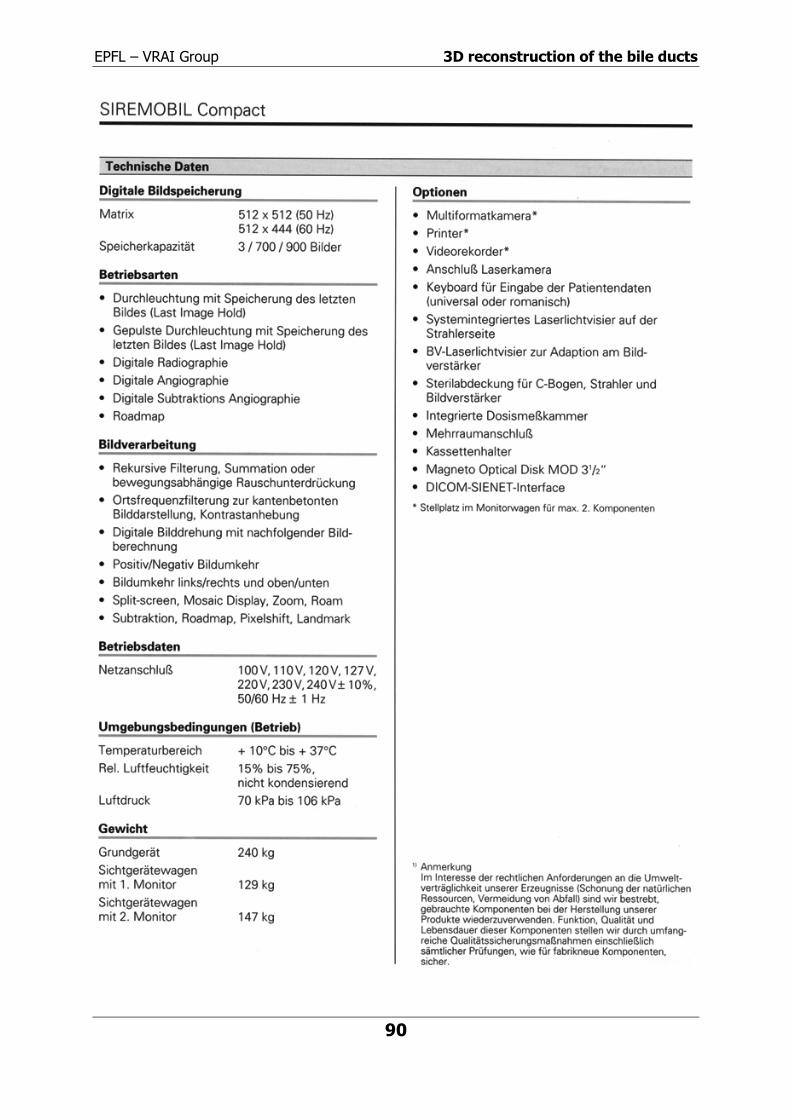
EPFL � VRAI Group 3D reconstruction of the bile ducts
90

EPFL � VRAI Group 3D reconstruction of the bile ducts
91