m icrofinance a s a j ob c reator e vidence from e …...m icrofinance a s a j ob c reator – e...
TRANSCRIPT

MICROFINANCE AS A JOB CREATOR – EVIDENCE FROM EASTERN EUROPE
Eva Erhardt
Johannes Gutenberg University Mainz, Germany
This version:
July 2016
Abstract
This paper examines the impact of microfinance on job creation. The growth of small businesses be-yond self-employment through microcredit has so far been rarely studied, in particular for Eastern Europe. We use a unique panel dataset which combines data from a large microfinance bank in Bul-garia with countrywide information on micro-, small- and medium-sized firms. By applying propensity score matching methods together with difference-in-differences, we find strong positive effects of mi-crocredit with respect to the number of employees in participating firms. In fact, the participants have on average 2.6 more employees two years after receiving a microcredit than matched non-participants. Related to the firm size before treatment, this translates into a relative growth difference in employees of 35 percent through microcredit. In addition, we show that the program effects are long-lasting. As a matter of fact, only an evaluation period of several years after treatment captures the sustainable impact of microcredit on firm size after initial upward and downward adjustments. Furthermore, we add support to the findings that smaller firms are more constrained by credit than are larger firms and that the point in time at which the impact occurs is affected by the loan purpose.
Keywords: microfinance, job creation, propensity score matching, Eastern Europe
JEL Classification Number: G21, J23, C21, P34
Contact details: Eva Erhardt, PhD student, Johannes Gutenberg University Mainz, Chair of Applied Statistics and Economics, 55099 Mainz, Germany, Email: [email protected]
1 INTRODUCTION Microfinance is deemed to be a strategy for creating jobs. The European-Union (2010) for example considers microfinance as one measure to increase employment levels in Europe until 2020. The rationale on which the promise to create jobs rests upon, is as follows: poor individuals could earn high marginal returns through business activities, but are credit constrained. Access to microcredit, typically defined as small loans to underserved entrepreneurs (Banerjee et al., 2015), helps realizing growth opportunities by starting or expanding businesses, and thus raising incomes and creating em-ployment (see Karlan and Morduch, 2010; McKenzie and Woodruff, 2008; De Mel et al., 2008).
Since job creation is a major concern for policymakers all over the world, this is one of the reasons why microfinance has become increasingly popular since its emergence in the mid-1970s. Micro-finance programs which provide microcredit next to other financial services such as micro-savings or micro-insurance are now widespread in low and middle-income countries and recently emerge in high-income countries as well. In total, about 200 million people worldwide are considered to be cli-
Preliminary Draft
Please do not quote without permission of
the author

Eva Erhardt / Microfinance as a job creator / 2
ents of some 3,600 microfinance institutions (Maes and Reed, 2012). Accordingly, vast amounts of public and private funds are committed to microfinance programs, for example USD 31 billion in 2013 (CGAP, 2015).
The growing importance of microfinance has resulted in a considerable number of impact studies (see surveys of impact assessments on microcredit by Duvendack et al., 2011; Stewart et al., 2012; van Rooyen et al., 2012; Pande et al., 2012; Grimm and Paffhausen, 2015 or Banerjee et al., 2015). Astonishingly however, evidence on the impact of microcredit on employment still remains very scarce. One reason is that many programs strive for other objectives than job creation such as in-come stabilization, consumption, poverty reduction or even empowerment of women. The existing studies which do assess programs aiming at employment creation are furthermore often limited to the impact of microcredit on self-employment. They focus on measuring for example the creation of new businesses or the number of hours worked by the microcredit borrower (e.g. Pitt and Khandker, 1998; Coleman, 1999; Dunn and Arbuckle, 2001; Coleman, 2006; Setboonsarng and Parpiev, 2008; Chemin, 2008; Attanasio et al., 2011; Duvendack and Palmer-Jones, 2012; Augsburg et al., 2012). The growth of existing small businesses in terms of employees through microcredit is less frequently studied (e.g. Montgomery, 2005; Bruhn and Love, 2009; Gubert and Roubaud, 2011; Angelucci et al., 2015 Banerjee et al., 2013; Crépon et al., 2014). While enabling self-employment is an important out-come, a larger contribution to job creation is only achieved if microcredit also increases wage-employment.
Another aspect which has been largely neglected in the literature so far is the assessment of micro-finance programs in Eastern Europe. This is in sharp contrast to the fact that in regional terms the former Soviet Republics of Eastern Europe and Central Asia have received the largest share of worldwide commitments to microfinance programs as estimated by CGAP (2015). As a matter of fact, the study by Augsburg et al. (2012) on the impact of a microfinance institution in Bosnia & Herze-govina on self-employment is the only existing impact assessment for the region. This is also prob-lematic for another reason. Microfinance programs in Eastern Europe have distinctive features which differentiate them from programs in other regions. Most of all, the microfinance sector in Eastern Eu-rope is dominated by so-called individual lending programs rather than group-lending which was orig-inally associated with microfinance. In Eastern Europe, microfinance institutions mostly lend to indi-vidual borrowers with some previous business experience (Armendáriz de Aghion and Morduch, 2000). Moreover, the region is characterized by a relatively large share of for-profit microfinance pro-viders such as microfinance banks and to a lesser extent credit unions. This fact is related to the de-velopment that during the transition period to market economies in the 1990s and early 2000s, when most microfinance institutions were founded in Eastern Europe, for-profit microfinance gained mo-mentum. Policymakers started arguing that new microfinance institutions should be financially sus-tainable and international donors increasingly preferred loans to grants for the establishment of micro-finance institutions (Hartarska et al., 2006; Caudill et al., 2009). A final characteristic of microfinance in Eastern European is its relatively large loan sizes of around USD 2,500 per client compared to a global average of USD 700 (MIX-Market, 2013). In part, this difference can be explained by the more advanced economic development of Eastern Europe compared to other regions and the link of loan sizes to local income levels. In addition, the larger loan sizes seem to result from a combination of individual lending schemes with the widespread provision of microfinance by banks which tend to lend in greater volume than other microfinance institutions such as non-governmental institutions (Cull et al., 2009).
This paper contributes to closing two research gaps simultaneously. It first adds to the scarce litera-ture on impact assessments of microfinance beyond self-employment by assessing the change in wage-employment in businesses of microcredit borrowers. The study furthermore contributes to the very limited evidence on the impact of microfinance in Eastern Europe since it assesses a micro-

Eva Erhardt / Microfinance as a job creator / 3
finance program in Bulgaria with typical features for the region. As a matter of fact, this study is to the best of our knowledge the first assessment of wage-employment effects in Eastern Europe of an indi-vidual lending program by a for-profit microfinance bank.
The unique combination of administrative data from the program as well as from a country-wide firm-level database for several years, enables us to apply propensity score matching methods extended by a difference-in-differences estimator. Our sample consists of a balanced panel dataset of 974 partici-pating firms which received a program loan in 2004 and 60,032 non-participating firms used for matching. We test the sensitivity of our results regarding variations within the matching process. We also assess their sensitivity to deviations from the identifying assumptions, in particular regarding selection on unobservables. Our results turn out to be robust and we find strong positive and signifi-cant effects of microcredit with respect to the number of employees in participating firms. In fact, par-ticipants have on average 2.6 more employees two years after receiving a microcredit than matched non-participants. Related to the firm size, this translates into a growth difference in employees of 35 percent for participants compared to matched non-participants. The dimension and direction of this positive effect also holds if we include further variables and longer time trends before treatment in our propensity score estimations. In addition, we show that the program effects last as long as six years after receiving the microcredit. At the same time, participants expand their number of employees very rapidly after treatment followed by a subsequent contraction in firm size. A sustainable new level of firm size that mirrors underlying financials is not attained until two years after treatment. Accordingly, only an evaluation period over several years after treatment seems able to capture the sustainable impact of microcredit on firm growth. Finally, heterogeneous effects for sub-groups point to the finding from other studies that smaller firms are more constrained by credit than are larger firms. In fact, the smaller a firm, the higher is the estimated impact of microcredit on its number of employees. Finally, we find that loan purposes in terms of working capital or fixed assets affect the point in time at which impacts occur. Therefore, it seems advisable to take the type of loan purpose into account when de-ciding over the appropriate evaluation period for a microfinance impact assessments.
The remainder of this paper is organized as follows: Section 2 provides a literature review on the im-pact of microfinance on job creation, an overview of access to finance for small firms in Bulgaria and a brief description of the program. Section 3 describes the data used in this study and presents descrip-tive results. Section 4 illustrates the identification strategy by focusing on the approach we adopted to control for selection biases. The main results of our estimations are then discussed in Section 5 which also contains an analysis of dynamic and heterogeneous effects. Finally, we present sensitivity tests of our results in Section 6 before we conclude in Section 7.
2 MICROFINANCE, SMALL FIRMS AND JOB CREATION
2.1 PREVIOUS IMPACT ASSESSMENTS ON MICROFINANCE AND EMPLOYMENT Recent years have seen a growing number of impact assessments for microfinance. In particular, the experimental evidence from randomized control trials is rapidly increasing. The expanding body of evidence has also resulted in a number of synthesis studies of microfinance impact assessment (see for example Duvendack et al., 2011; Stewart et al., 2012; van Rooyen et al., 2012; Pande et al., 2012; Grimm et al., 2015 and Banerjee et al., 2015). These studies discuss a particular type of program (e.g. micro-savings or programs in Sub-Saharan Africa) and try to generate overall conclusions on certain effects.
As far as effects on employment are concerned however, there still exists only a limited number of relevant studies in the literature. To begin with, the vast majority of the assessed programs is not de-signed to create employment in the first place. Rather, they aim at increasing income and consump-

Eva Erhardt / Microfinance as a job creator / 4
tion, poverty reduction and even various other outcomes such as school attendance of children or empowerment of women (Armendáriz de Aghion and Morduch, 2010). This is particularly the case for so-called group lending approaches from economically less developed regions which dominate the body of evidence and require borrowers, often women with no previous business experience, to form small groups for joint lending and repaying. In total, about twenty studies exist which assess the im-pact of microcredit on employment. They are summarized in Table 1 including information on the country where the assessed program is located, a brief description of the program, the applied re-search design and the type of effects on employment outcomes.
(Table 1 about here)
A first finding from the last column of Table 1 is that many of the impact studies focus only on self-employment effects of microcredit. They measure for example the number of hours worked by the borrower and other members of the borrower’s household or the creation of new businesses. In con-trast, the growth of already existing small businesses in terms of employees through microcredit is less frequently studied. While enabling self-employment is an important outcome, a larger contribution to job creation is only achieved if microcredit also increases wage-employment.
A second insight emerging from the existing evidence is that the impact of microcredit on employment is very mixed as also indicated in the last column of Table 1. Some studies find positive impact on employment. For instance, Binswanger and Khandker (1995) as well as Burgess and Pande (2005) deal both with the impact of a policy in India to increase the supply of microcredit to rural areas. They find that the expansion of rural credit supply was associated with an increase of employment in non-agricultural sectors together with a rise in agricultural wages. Abou-Ali et al. (2010) assess the impact of a microfinance program under the Egyptian Social Fund for Development. They find a very positive effect on self-employment in urban areas and a more modest effect on wage-employment, particularly in rural areas. Attanasio et al. (2011) find that access to group loans among households in Mongolia increased the likelihood of owning an enterprise by 10 percent more than in control villages. For indi-vidual lending on the other hand, they detect no significant increase in enterprise ownership. Bruhn et al. (2009) show that the opening of a new microcredit bank in Mexico led to an increase in the number of informal business owners by 7.6 percent. Total employment also increased by 1.4 percent. Augsburg et al. (2012) focus on self-employment in an impact assessment with a microfinance institution in Bosnia and Herzegovina. They find that households of borrowers are 6 percentage points more likely to receive income from self-employment than households in the control group. Hours worked by household members of the borrower on the other hand did not change significantly.
In contrast, results of other impact assessments show that microcredit does not have a significant impact on employment or even reduces employment levels. Coleman (1999) and Coleman (2006) for example do not find any significant impact on self-employment for a group-lending program to rural households in Thailand. Gubert et al. (2011) did neither find an impact on the number of employees in businesses of microcredit clients for a program in Madagascar. Angelucci et al. (2015 did not find any effect on either business ownership or the number of employees for a program in Mexico. In a similar manner, Crépon et al. (2014) do not find any impact of microcredit on either the creation or the ex-pansion of businesses for a program in rural Morocco. Banerjee et al. (2013) evaluate a lending pro-gram in slums of Hyderabad in India. They find no positive impact of microcredit on the number of employees for clients with existing businesses before treatment and even negative impact for clients with new businesses with 0.2 fewer employees for treatment than control areas. Because the new businesses in treatment areas also have lower profits than in control areas, they argue that micro-credit might have a negative selection effect. It might draw individuals into new entrepreneurship who have actually less propensity to become successful entrepreneurs than existing entrepreneurs. Karlan and Zinman (2011) additionally find negative effects for a microcredit program in the Philippines on the number of business activities. Also the number of employees in the treatment group decreased

Eva Erhardt / Microfinance as a job creator / 5
relative to controls. In fact, treatment group business owners operate 0.1 fewer businesses (7 per-cent) than the control group and have 0.27 (31 percent) fewer paid employees.
In some cases, the impact even varies for identical datasets if different research designs are applied. This is the case for a set of studies which are all related to a dataset on group-lending programs for poor rural households in Bangladesh. The original study was conducted by Pitt et al. (1998) and trig-gered a vivid academic debate on methodological issues. As for impact on employment, all of the related studies estimate hours of market labor supply, which is the hours engaged in productive activi-ties outside of the household. Pitt et al. (1998) find a positive impact of microcredit on hours of market labor supply for female borrowers and negative impact for male borrowers. Chemin (2008) later ap-plied propensity score matching to the same data. He found that participating men work more, where-as the effect for women is insignificant. In another re-estimation of the same data with propensity score matching and additional tests of sensitivity to unobservables, Duvendack et al. (2012) show that the impact is insignificant for both female and male labor supply. In a similar manner, Montgomery (2005) found for a microfinance institution in Pakistan that its microcredit program had a very positive impact on employment levels of borrowers’ businesses. A later study by Setboonsarng et al. (2008) who applied propensity score matching to the same dataset, found a less strong impact on employment. Another example for different impacts depending on the research design is the study by Dunn et al. (2001) on a program in Peru. They find that microcredit had a positive impact on the total days worked per month in borrowers’ micro-businesses for household members and non-members. Tedeschi and Karlan (2010) re-estimate the impact in Peru by additionally accounting for dropout of clients from the program between the baseline and follow-up survey. They find that total employment over the top three enterprises operated by an existing client was over-estimated. Whereas Dunn et al. (2001) find that employees in microenterprises of a borrower have 14.6 more days worked per month, the re-calculation estimates an increase of only 4 days per month.
The mixed impact of microfinance on employment is also reflected in the findings of the synthesis study by Grimm et al. (2015). They conclude that only 20 out of 54 impact estimates from studies dealing with improved access to finance (including microcredit) show a statistically significant positive effect on employment. 32 impact estimates were statistically not significant. In 2 cases, a statistically significant negative effect on employment was even found. Overall, the programs under consideration were more effective in creating new firms than expanding existing employment.
Probably most important, a third striking insight from the existing literature on microcredit is that from a regional perspective the evidence for Eastern Europe is particularly scarce. As a matter of fact, the study by Augsburg et al. (2012) on self-employment at the household level for microcredit clients in Bosnia and Herzegovina is the only existing impact assessment for microfinance according to the synthesis studies for the transition economics of Eastern European and Central Asia. Some additional evidence for Eastern Europe related to our study comes from two programs beyond the scope of im-pact surveys on microfinance. Brown and Earle (2010) evaluate the effectiveness of small loans from a program by the U.S. development agency (USAID) for firms in Romania. The authors apply propen-sity score matching to estimate the impact on employment, sales, and survival for about 300 firms and conclude that the program loans raise employment. Another study of a USAID program in Macedonia by Bah et al. (2011) focuses on the impact of technical assistance for small- and medium-sized firms rather than financial support, but is comparable to our paper in terms of research design. Overall, Bah et al. (2011) find that technical assistance raised employment by 16–20 percentage points in the first year after assistance and by 26–30 points by the third year.
Largely neglecting the Eastern European region in impact assessments of microcredit is problematic for several reasons. To start with, it is undesirable in terms of accountability for public and private funds, since Eastern Europe and Central Asia used to receive the largest share of worldwide com-mitments to microfinance as estimated by CGAP (2015). In addition, Eastern Europe deserves more
Eva Erhardt / Microfinance as a job creator / 6
attention because its microfinance programs have distinctive features which differentiate them from programs in other regions. Most of all, the microfinance sector in Eastern Europe is dominated by so-called individual lending programs rather than group-lending which was originally associated with microfinance. In Eastern Europe, microfinance institutions mostly lend to individual borrowers with some previous business experience (Armendáriz de Aghion et al., 2000). Moreover, the region is characterized by a relatively large share of for-profit microfinance providers such as microfinance banks and to a lesser extent credit unions. This fact is related to the development that during the tran-sition period to market economies in the 1990s and early 2000s, when most microfinance institutions were founded in Eastern Europe, for-profit microfinance gained momentum. Policymakers started arguing that new microfinance institutions should be financially sustainable and international donors increasingly preferred loans to grants for the establishment of microfinance institutions (Cull et al., 2009; Hartarska et al., 2006; Caudill et al., 2009). A final characteristic of microfinance in Eastern European is its relatively large loan sizes of around USD 2,500 per client compared to a global aver-age of USD 700 and only USD 200 in South Asia (MIX-Market, 2013). To some extent, this difference can be explained by the more advanced economic development of Eastern Europe compared to other regions and the link of loan sizes to local income levels. In addition, the larger loan sizes seem to result from a combination of individual lending schemes with the widespread provision of microfinance by banks which tend to lend in greater volume than other microfinance institutions such as non-governmental institutions (Cull et al., 2009).
To summarize the existing literature, evidence on the impact of microcredit on job creation is still lim-ited, in particular for employment effects beyond self-employment. The studies which do focus on business expansion and the creation of wage-employment moreover get very mixed results. Most astonishingly, the Eastern European region has been largely neglected by the literature on the impact of microcredit despite its notable position in terms of international financial support as well as particu-lar regional characteristics of microfinance. Therefore, this study contributes to closing two research gaps simultaneously. On the one hand, it adds to the scarce literature on wage-employment effects of microfinance. By providing evidence for a microcredit program from a for-profit microfinance bank in Bulgaria consisting of relatively large, individual loans to small businesses, this study on the other hand also contributes to the very limited evidence on the impact of microfinance in the transition economies of Eastern Europe and Central Asia.
2.2 ACCESS TO FINANCE FOR SMALL FIRMS IN BULGARIA The economic theory on which the impact of microcredit on employment rests upon is that entrepre-neurial individuals could engage in profitable business activities, but they are credit constrained. Ac-cess to microcredit is supposed to help overcome these credit constraints and realize growth opportu-nities by starting or expanding businesses, and thus creating employment. To investigate the impact of a microfinance program, it is therefore necessary to identify an adequate group of credit-constrained firms that do not participate in the program and compare them to the firms that partici-pate. The purpose of this section is to discuss if such an adequate control group can be found in our research context.
One might argue that ideally neither participants nor non-participants should have any previous ac-cess to finance before start of the program and that moreover non-participants should also remain without any access to finance during the evaluation period. In reality, it is very unlikely to find firms which are totally excluded from the financial sector and it is not even a necessary condition to some extent. Most businesses have at least access to informal sources of finance such as moneylenders or family and friends. Research shows however that informal financial institutions co-exist with micro-finance and play a complementary role to the formal financial sector offering small, unsecured, short-term loans (Ayyagari et al., 2010; Guirkinger, 2008). According to this view, informal financial institu-

Eva Erhardt / Microfinance as a job creator / 7
tions rely on relationships and reputation and cannot substitute for formal financial systems, because their monitoring and enforcement mechanisms are ill equipped to scale up and meet the needs for larger and long-term investments. Microfinance’s promise to create employment by enabling invest-ments in profitable business opportunities seems therefore independent of the existence of an infor-mal financial sector. As far as access to loans from the formal financial sector is concerned, we none-theless need to take great care of discussing its availability to the control group in our study.
The data available for our empirical analysis contains information on access to formal loans from the program lender ProCredit Bank Bulgaria before and during the evaluation period. Accordingly, we are able to exclude any firms from the control group of non-participants which had access to loans from ProCredit Bank. Since ProCredit Bank was the largest provider of microfinance in Bulgaria as shown below, we control for the most important source of formal finance for small firms in Bulgaria. Further-more, we chose a context in terms of country and time period where access to formal finance was in general still very limited for most firms as is also shown in more detail below. Since however the data does unfortunately not inform us on access to loans from any other banks or microfinance institutions, we next provide an overview on the availability of bank credit during the period under review.
It is worth noting that the availability of alternative credit to non-participants is an issue that other impact assessments of microcredit must deal with as well. Banerjee et al. (2013) for example describe in their experiment in India that at baseline almost no microcredit was available, although about two-third of the sample households had at least one loan outstanding from informal financial sources. During the treatment however, other microcredit programs also started operations in both treatment and control villages. They suggest that in order to interpret differences between treatment and control areas as due to the microcredit program, it must only be the case that borrowing is at least higher in treatment than in control areas. We have good cause to assume that this is the case for our group of participants compared to non-participants. Brown et al. (2010) furthermore argue in their evaluation of a program in Romania that if control firms receive loans from other providers and if effects of these loans are positive, then this would only imply that the estimates of program effects are understated. In our case this implies that if we find a positive impact of microcredit from ProCredit Bank on employment, then most likely loans from other financial institutions would have a positive effect as well. In case that a certain share of control firms benefits from alternative loans, we would rather under-estimate the positive effect of the program loans on participants.
2.2.1 THE DEMAND SIDE
Having expressed methodological considerations on the availability of formal credit for non-participants, the demand side of finance deserves attention first. The target group of the microfinance program under review are micro-enterprises (with less than 10 employees). More precisely, a vast majority of 78 percent of the microcredit clients in our sample were micro-enterprises at the start of the program. Further 20 percent were small enterprises (with less than 50 employees) and 2 percent were medium-sized enterprises (with up to 250 employees).1 Many statistical sources treat micro-, small- and medium-enterprises (MSMEs) as one group of firms in contrast to large enterprises with 250 employees and more. To keep it simple for our purposes, we will apply the term small firms when referring to this group of firms with up to 250 employees.
By 2003 – the starting point of the period under review - there existed around 240,000 micro, small and medium-sized enterprises in Bulgaria according to data from EU (2008). Small firms were consid-ered the engine of the Bulgarian economy: according to the 2004 annual report on small and medium- 1 As defined by EU (2005), next to the threshold of 250 employees, micro, small and medium-sized firms should
also not have an annual turnover of more than EUR 50 million or a balance sheet of more than EUR 43 million.
Eva Erhardt / Microfinance as a job creator / 8
sized enterprises of the Ministry of Economy (2004), they constituted 99 percent of all enterprises in Bulgaria (90 percent were micro-enterprises), generated 79 percent of the employment, accounted for 75 percent of the turnover and 61 percent of the added value of private enterprises.
Bulgaria is not an exceptional case in that regard. de Kok et al. (2011) show that small firms account for 99.8 percent of non-financial enterprises in the European Union with the overwhelming majority of 92 percent being micro-enterprises. Micro, small and medium-sized enterprises employ two-thirds of the formal EU workforce. 30 percent of total EU employment is attributable to microenterprises, 20 percent to small enterprises and 17 percent to medium-sized enterprises. Between 2002-2010, 85 percent of total net employment growth was created by small firms.
The general economic context for small firms in Bulgaria had improved by 2003 after more than a decade of transition to a market economy. Bulgaria had a population of 7.8 million, GDP grew at 5.4 percent, unemployment amounted to 13.7 percent and it was classified as lower middle income coun-try. In 2007, Bulgaria became a new member of the European Union. Still, Bulgaria’s GDP per capita remains among the lowest in Europe and about 20 percent of the Bulgarian population is living in relative poverty.2
In constrast to the vital importance of small firms for the Bulgarian economy, they had difficulties to access formal finance. A survey by the Bulgarian SME Promotion Agency in 2002 shows for example that 67 percent of the small and medium-sized firms had no access to bank financing (BSMEPA and NOEMA, 2011). A survey by the Worldbank (2006) confirms that in 2002 only 16 percent of 200 interviewed Bulgarian firms used formal borrowing from the financial sector for new investments (21 percent in 2005). Not surprisingly, access to finance is reported as a major constraint to firm growth. Another survey of managers from 506 small and medium-sized enterprises in 2003 points into the same direction: the shortage of financial resources for investment, renovation and working capital is considered as the major barrier to growth by small Bulgarian firms (BSMEPA and CED, 2004). Pissarides et al. (2003) analyze the principal constraints of small and medium enterprises in Bulgaria and Russia, using data from a survey of 437 top managers, who also identified the lack of external financing as a particularly serious constraint. In addition, Budina et al. (2000) investigate if investment decisions of 1,000 medium and large Bulgarian firms in the period 1993-1995 were constrained by liquidity, and if these constraints varied by firm size. They show that firms were constrained and the smaller the firms, the larger were their liquidity constraints.
Evidence across other countries adds further support to the fact that firms are often credit constrained and smaller firms are more constrained than larger firms. Ayyagari et al. (2008) show that of ten ob-stacles in the business environment that firms report, only three emerge from the regressions as bind-ing constraints with a direct association to firm growth: lack of finance, crime, and policy instability. The finance result is shown to be not only the most robust, but also to have the largest direct effect on firm growth. As for firm size, the authors find smaller firms to be more constrained by financing obsta-cles than larger firms. Beck et al. (2005) compare the relative effect of lack of finance, corruption, and legal obstacles on firm growth. They also find that the significance of growth constraints varies con-siderably with firm size. It is consistently the smallest firms that are most constrained. For small firms the financing obstacle has even almost twice the negative effect on annual growth than it does for large firms. Beck et al. (2008) show that small firms finance on average 13 percentage points less of investment with formal bank finance compared to large firms. In a related study Beck et al. (2006) focus specifically on the determinants of financing obstacles and find that younger, smaller and do- 2 Economic indicators are based on data from Worldbank. Available at: http://data.worldbank.org/country/bulgaria
(Accessed: 16 November 2015). GDP per capita was USD 2,697 in 2003 and USD 7,499 in 2013. 22 percent of the population was living below the national poverty line in 2006 and 21 percent in 2013 (based on popula-tion-weighted subgroup estimates from household surveys).

Eva Erhardt / Microfinance as a job creator / 9
mestic firms report higher obstacles. When considering the effect of country characteristics, they fur-thermore show that firms in countries with higher levels of financial development, more liquid stock markets, more efficient legal systems and higher GDP per capita report lower financing obstacles.
For Europe, Hutchinson and Xavier (2006) compare the middle-income country Slovenia to the high-income country Belgium. They find that small firms in Slovenia depend more on internal cash flow for investments and are thus financially more constrained than large firms in Slovenia as well as than their counterpart small firms in Belgium. Hartarska and Nadolnyak (2008) compare for Bosnia and Herzegovina the investment sensitivity to internal funds of micro-enterprises in municipalities with significant presence of microfinance institutions to that of micro-enterprises in municipalities with no (or limited) presence of microfinance institutions. Their results indicate that microfinance alleviated financing constraints of micro-enterprises.
2.2.2 THE SUPPLY SIDE
The above presented evidence points to the fact that the lack of access to finance constrains the growth of small Bulgarian firms. After the demand side, the supply of formal financing from the banking sector as well as from the microfinance sector is considered in more detail. By the start of the period under review in 2003, the Bulgarian banking system had recovered from several crises during the beginning of the transition to a market economy. Since the introduction of a currency board in 1997, the Bulgarian Lev (BGN) was pegged to the euro at 1.95583:1. The Bulgarian banking sector consisted of 29 banks and 6 branches of foreign banks. Foreign ownership dominated (19 of the 29 banks) and all but 2 banks were private. While the banking sector was still relatively small with a ratio of domestic credit to the private sector (as percentage of GDP) of 26 percent in 2003 compared to Western countries such as Germany with 110 percent or the U.S. with 177 percent,3 bank credit experienced rapid real growth of 40 percent as in most other countries in Eastern Europe. The risk-averse behavior of banks during the early transition period, gradually gave way to increased lending aided by economic recovery and privatization of state banks (Duenwald et al., 2005).
Notwithstanding the overall expansion of bank credit, financing for small firms remained limited as the following evidence suggests: Duval and Goodwin-Groen (2005) estimate that in 2001 banks had col-lectively extended only around 16,000 business loans under EUR 100,000 to the total of Bulgarian enterprises (about 240,000 including large firms). Anecdotal evidence from the program points into the same direction. As described in ProCredit Bank Bulgaria’s annual report 2004 ‘in October 2001, when the bank was founded, traditional banks in Bulgaria were still extending loans to small and medium-sized enterprises only in exceptional cases. The conventional commercial banks often focus their lending operations on corporate finance and consumer lending, but tend to neglect small businesses as a potential clientele. Their main reasons for not lending to micro, small and medium-sized enterprises are the perceived inadequacy of MSMEs’ accounting methods, their ostensible inability to provide sufficient collateral and the high administrative costs incurred in small business lending.’ In terms of market share of Bulgarian banks in the segment of small business lending, a survey by BSMEPA et al. (2004) covering 8 out of 29 banks provides the following insight. Out of a total of 13,771 loans extended to small- and medium-sized firms by the surveyed banks in 2003, ProCredit Bank Bulgaria is the largest provider in terms of number (5,560 loans amounting to 66,400,000 BGN) and United Bulgarian Bank in terms of volume (4,537 loans amounting to 310,205,000 BGN).
3 See World Bank, http://data.worldbank.org/country/bulgaria (Accessed: 16 November 2015).

Eva Erhardt / Microfinance as a job creator / 10
Next to banks, the microfinance sector constitutes another source of formal finance for small firms. According to data from MIX-Market4 the gross loan portfolio of microfinance institutions in Bulgaria in 2004 was worth about USD 200 million and there existed about 37,000 active microfinance borrow-ers. The microfinance sector was largely dominated by ProCredit Bank Bulgaria, making up for more than 90 percent of the loan portfolio and 77 percent of active borrowers. Other providers during this period were only a few microfinance institutions, most notably Nachala, USTOI and Mikrofond.
Regarding the earlier question if an adequate control group in terms of limited access to formal fi-nance can be found in our research context, the following can be noted: Only about one third of micro, small and medium-sized firms in Bulgaria indicated any access to formal finance in 2002 before start of the program (BSMEPA et al., 2011). This is an average value, while evidence points to the fact that access to loans for micro- and small firms is even much lower than for medium-sized firms (e.g. Budina et al., 2000; Hutchinson et al., 2006; Ayyagari et al., 2008; Beck et al., 2005). In addition, ProCredit Bank Bulgaria was by far the largest provider of microcredit in the microfinance sector and one of the largest providers within the banking sector. The rapid expansion of the bank’s lending operations to small firms as described below and its large market share can be regarded as a further indicator for the limited access to finance of small firms in Bulgaria during the period of evaluation. Moreover, small firms indicating access to bank loans were to a considerable extent clients of ProCredit Bank and can be consequently excluded from the control group. Finally, if some control firms received loans from other providers than ProCredit Bank and if loan effects are positive, we should slightly under-estimate the impact of the program.
2.3 THE PROGRAM - PRO CREDIT BANK BULGARIA The program assessed in this paper consists of microcredit provided to small firms by ProCredit Bank Bulgaria.5 The bank represents many of the characteristics which are typical for microfinance in East-ern Europe as introduced in section 1. ProCredit Bank Bulgaria is a full-service microfinance bank.6 It is part of ProCredit Group which consists of further banks in Eastern Europe, Latin America and Ger-many. The bank was established in 2001 by international investors. As expressed by the chairman of its supervisory board in the bank’s first Annual Report 2001,7 the establishment was motivated by the undersupply of credit to micro, small and medium-sized businesses in Bulgaria and the opportunities that these circumstances provide. Furthermore, the mission statement specifies the focus on lending to micro, small and medium-sized enterprises out of a conviction that these businesses create the largest number of jobs and make a vital contribution to the economy. Job creation which will be as-sessed in this paper is therefore a specific objective of the program. While the investors do not expect short-term profit maximization, the bank is supposed to achieve a sustainable return on investment and hence belongs to the segment of for-profit microfinance banks typical for Eastern Europe. The bank follows an approach of individual lending to entrepreneurs with a minimum market experience of 6 months. As typical for micro-enterprises, clients often lack official financial statements and collateral. Consequently, the bank developed a lending technology based on a personnel-intensive analysis of
4 MIX-Market is a not-for-profit organization that d collects data on microfinance institutions to promote infor-
mation exchange. Available at: http://www.mixmarket.org/mfi/country/Bulgaria (Accessed: 16 November 2015). 5 More information on ProCredit Bank Bulgaria is available at: http://www.procreditbank.bg/en (Accessed: 16
November 2015). 6 This characterization holds for the period of our evaluation. After the financial crisis of 2007/2008, ProCredit
Group introduced a strategic shift away of its original mission as microfinance provider to positioning itself as a provider of a wider range of modern financial services (e. g. e-Banking, cards, payroll, trade finance) for small businesses.
7 Available at: http://www.procreditbank.bg/uploads/AnnualReports/2001godina.pdf (Accessed: 13 April 2016).

Eva Erhardt / Microfinance as a job creator / 11
the borrower’s business including a personal visit by the loan officer to confirm the financial situation before loan approval as well as regular monitoring visits during the course of the loan. Its lending op-erations expanded rapidly. The bank started in 2001 with 955 loans worth about EUR 5 million. In the beginning of the period under review in 2004, it had already a total of 19,390 business loans outstand-ing worth EUR 127 million. By 2010, the end of the review period, the bank had 31, 675 business (and agricultural) loans outstanding worth EUR 533 million. Accordingly, the average loan size for business loans is relatively large even for Eastern Europe (5,236 in 2001, 6,550 in 2004 and 16,827 for 2010). As for geographical outreach, ProCredit Bank Bulgaria started operations with 7 branches. The net-work grew to 35 branches by the end of 2004 covering 19 out of 28 Bulgarian districts. In 2010 the country-wide network amounted to 75 branches and outlets.
3 DATA Our empirical analysis is based on all firms that have received their first business loan from ProCredit Bank Bulgaria in the year 2004 and year-end data on Bulgarian firms from 2000 to 2010. This section contains more information on the sample of participating and non-participating firms. It describes the sources and construction of our panel dataset and provides basic descriptive statistics on sample characteristics.
3.1 FIRM-LEVEL DATASET We use a unique dataset which we constructed by matching two different sources: (i) program data from ProCredit Bank, and (ii) a Bulgarian firm-level dataset. The program data was generated using the bank’s Management Information System. The data includes loan and respective client data. The loan data (e.g. amount, date of disbursement, loan purpose, interest rate, maturity) is generated au-tomatically by the information system as soon as a loan is disbursed. The client data is collected through personal client assessments by the loan officers. Information on location, industry and legal form is available for all clients. Financial data as well as the number of employees is on the other hand only available for about 75 percent of the clients. Since this information is furthermore only rec-orded at the time of loan approval and usually not updated unless a follow up loan is approved, a development over time cannot be tracked. Consequently, the program data is used to identify the sample of participating program clients and obtain detailed loan information. As for all other infor-mation such as client’s characteristics, their number of employees and financial data, we rely on the second data source. As Heckman et al. (1997) point out, the use of one single source of information for characteristics of both participants and non-participants largely reduces estimation bias in impact studies.
Regarding the timing of treatment, we restrict our attention to firms treated in the year 2004. We de-fine treatment as disbursement8 of a credit from ProCredit Bank between 1 January and 31 December 2004. The decision to focus on 2004 results from a trade-off between the availability of formal finance for the control group and data availability. On the one hand, we picked an early period of the bank’s operations with still limited availability of loans from other banks to non-participating firms, since credit markets largely expanded over time. The intention is to be better able to attribute and less under- or overestimate the impact to microcredit as explained in Section 2. On the other hand, we were not able to choose yet earlier years of operation (the bank started in October 2001), because the data availa-bility in the firm-level dataset sharply reduces when going further backwards in time. We furthermore
8 One could argue that firms already start hiring employees at loan approval. While we do not have information
on the date of loan approval, we know that on average only 9 days elapsed in total between loan application, approval and disbursement. It thus does not seem to make a large difference which date to use.
Eva Erhardt / Microfinance as a job creator / 12
choose to focus on new clients only, i. e. firms that have not benefitted from earlier loans of the bank, because the first loan is most likely to best kick-start a process of growth. Firms in our control group did not receive a microcredit by ProCredit Bank in any year prior to or during our main evaluation pe-riod.
As far as the time span over which impacts are estimated is concerned, the firm level database pro-vides us with year-end data (31 December) from 2000 until 2010. Our baseline data hence dates from 31 December 2003 just before start of the treatment on 1 January 2004. We allow the effects of hav-ing received treatment in 2004 to take several years to materialize. To this end, we examine the out-come variable two years after treatment, that is at the end of 2006. In the results section 5.3 we will additionally show the dynamic development of the treatment effect for other time periods. We focus on 2006 as our main point in time for the evaluation of effects, since the average duration of program loans was 24 months. The end of the main evaluation period is accordingly defined as 24 months after disbursement of the last program loan on 31 December 2004, which is the end of 2006. In fact, many impact studies of microfinance programs consider a period of about 24 months after treatment for measuring outcomes (for example Bruhn et al., 2009; Crépon et al., 2014 or Karlan et al., 2011).
To further construct our sample, we cleaned the dataset by loan purposes and kept only loans for business purposes. We deleted loans for consumption and housing, because we assume that non-productive loans for private purposes will not have an impact on labor demand in clients businesses. The core business loan products in 2004 were the micro-loans ‘Sprint’ and ‘Dynamo’ which accounted for about 90 percent of the business loans. The Sprint loan was especially popular, because no col-lateral was required and applications took only 24 hours to process. The average outstanding balance of a business loan was roughly EUR 5,000 and it was granted on average for a period of 24 months.
In total, the microfinance bank disbursed business loans to 9,270 new clients in 2004, of which 1,153 were legal entities as opposed to private individuals.9 We need to limit our analysis to legal entities, because our second data source, the Bulgarian firm-level dataset, is not containing any information for private individuals. Still, the number of participating firms is high compared to the majority of mi-crocredit impact assessments.
The second source for our dataset is the firm-level database Amadeus, created and distributed by the Bureau Van Dijk. It contains financial and other information on micro, small, medium and large public and private companies in Europe. The data is collected by local information providers. For Bulgaria, data is provided by Creditreform Bulgaria OOD, whose main source in turn is the National Statistical Institute. Additional surveys are conducted by Creditreform to both complete and cross-check data from the National Statistical Institute. Information on the number of employees per firm originates from the National Social Security Institute. This means, that only formal jobs for which firms pay social se-curity, are accounted for. Fortunately, the Amadeus data contains a very large number of micro-enterprises with less than 10 employees unlike many other sources for firm data. This is a decisive advantage for our purposes, since the majority of microcredit participants are micro-enterprises.
The Amadeus database contains year-end firm-level information on registered Bulgarian enterprises since 2000. The coverage of firms in terms of number and characteristics increases for more recent years. In 2004, the year of our treatment, the database contains in total 106,894 records which is a about 50 percent of all Bulgarian firms. We can only use those firms for our research with information 9 The large number of private individuals among business loan clients includes for example doctors or farmers
who do not need to register their businesses. It also includes owners of registered businesses who received small loan amounts for their business as private individuals, because it often took the authorities very long to issue the documents necessary for loan application of businesses. Since the bank provided us with information on the businesses which are related to a private individual and vice versa, we could further clean our dataset for business clients in 2004 who have already received a microloan as a private individual in previous years.
Eva Erhardt / Microfinance as a job creator / 13
on the output variable number of employees, both before and after treatment. In addition, we need further information on observable firm characteristics such as location, sector of activity, ownership type or gender of firm owner before treatment. Data on sales or profits is available to a much lesser extent and we thus decided to not consider it as requirement for forming our sample.10 Moreover, we eliminated any firms receiving a loan from ProCredit Bank prior or during the main evaluation period (about 4 percent of control firms between 2001-2006). This leaves us with 61,692 firms.
We matched both datasets using the national identification number of each firm. We could identify a large majority (87 percent) of the bank clients in our sample from 2004 in the Amadeus database. Data on the variables used for our empirical strategy of matching (number of employees, location, sector, ownership type and gender of owner) is available for almost all identified participants (97 per-cent). In a next step, we excluded large firms form the sample, because they are too few to carry out precise estimations and were not the target group of microloans in the first place. We also control for outliers in terms of change in employees.11 Eventually, we obtain a considerably long, balanced panel dataset of 974 participating firms and 60,032 non-participating firms with annual information before, during and after treatment on number of employees, sector, location, ownership type and gender of owner.
The dataset has three important advantages: First, sample size for both participants and non-participants is very large. The number of non-participating firms relative to the number of participating firms amount to 62:1. As we will apply propensity score matching, this increases the likelihood of find-ing one or more non-participating firms that are very similar, if not identical, to each of the participating firms. Moreover, compared to other evaluations of microfinance or small loan programs, we have a large number of participating firms as well. Among other things, this enables us to analyze sub-groups of participants in terms of firm size, loan features and geographic location for heterogeneous program effects. Second, the panel structure of the dataset allows us to use a difference-in-differences ap-proach which controls for time-constant unobservables that may have determined the participation in the program and the respective performance of firms. In section 4.1 we will further elaborate on this advantage. A third significant feature of the dataset is that it allows us to track the development for both participants and non-participants after treatment in terms of firm exit. In other words, we can identify, if and when a firm in our sample went out of business. Instead of losing these firms for our analysis, we can consider their exit in our estimations. Specifically, the Amadeus database contains historical records of inactive companies. We assume that a certain firm went out of business if no more data on employees or financials is available from a specific year onwards until the final reported year 2010 in the database. We consequently set the values for employees to zero for such a firm from the year of exit onwards. A firm exit during the evaluation period then results in a negative change rate of employees. This way, we can avoid the common survivor bias in panel data related to attrition of sample firms.
Table 2 shows firm exit rates for participants and non-participants separately. Exit rates are much higher among non-participants during the evaluation period 2004-2006. The cumulative exit rate for participants amounts to 2.9 percent until the end of 2006, while the corresponding rate for non-participating firms is 13.7 percent. Interestingly, for later years from 2007 onwards, the exit rates in-crease in particular for participants and become very similar to non-participants. One explanation
10 Only medium-sized and large enterprises are obliged to file accounts which would contain information on sales
or profit according to Creditreform. 11 We excluded 1 large firm from the treatment and 590 large firms from the control group. In terms of outliers, we
deleted firms with a relative change of 5,000 percent or more in employees from 2003-2006 (35 firms from the control and none from the treatment group) as well as firms with an absolute change of 300 or more employ-ees from 2003-2006 (31 firms from the control and none from the treatment group).

Eva Erhardt / Microfinance as a job creator / 14
could be decreasing effects of microcredit over time on firm survival. Since average exit rates in-crease for all firms in our sample, this also be triggered by the accession of Bulgaria to the European Union in 2007 and increased competitive pressure in particular on small domestic firms. Finally, the effects of the global financial crisis on small firms also start to increasingly show from 2007/2008 on-wards.
(Table 2 about here)
The main limitation of the dataset is that it does not provide us with more information on outcome variables such as sales, profit, assets or even data on part-time employment and wages. The litera-ture on small firm growth points to the fact that for very small firms, it usually takes a long time to in-crease one more formal employee or as Coad and Hölzl (2010) put it ‘indivisibilities are substantial for very small firms.’ They argue that growth effects of microcredit in terms of formal employees will thus not quickly show. Here it would be good to have information on part-time employment or sales which usually mirrors growth faster. In addition, it would be interesting to see how profitability, the accumula-tion of assets or wage levels are influenced by microcredit. Finally, another constraint is that we need to work with limited data for most of the firms in our sample as concerns pre-treatment trends, be-cause information on employees and financials such as sales or profit for earlier years than 2003 is only available for a reduced number of observations. Longer time trends together with additional firm characteristics to match upon such as qualification of employees or firm age would add further strength to robustness of results.
3.2 DESCRIPTIVE STATISTICS Table 3 provides the descriptive statistics measured at entry into the microcredit program at the end of 2003 separately for participants and for non-participants.
(Table 3 about here)
Looking at the participants of the microcredit program first, 78 percent were micro-enterprises with a size of less than 10 employees.12 20 percent were small firms with 10-49 employees and 2 percent were medium-sized enterprises with 50-249 employees. The only 1 large firm with more than 250 employees among participants was eliminated from the sample. On average, participating firms had 7.492 employees with a standard deviation of 13. Compared to non-participants, there is a considera-ble size difference. In fact, participating firms were almost only half the size of average non-participating firms with 12.737 employees and a standard deviation of 26. This size difference is also reflected in the distribution of firms within the three size categories micro, small and medium. Non-participating firms have a slightly larger share of medium- and small-sized firms. This is in line with our expectations that the target group for microcredit is very small companies and the firm size of partici-pants is smaller than for the average Bulgarian firm.
In terms of sectoral breakdown, about half (49 percent) of the microcredit is lent to trade companies (NACE section ‘wholesale and retail trade; repair of motor vehicles’), 17 percent into the manufactur-ing sector, and 10 percent into transportation. Real Estate activities and hotels/restaurants represent-ed only 7 and 5 percent of the participants respectively. Other sectors such as agriculture or construc-tion had a share of less than 5 percent each within the group of participating firms. Relative to non-participants, participants were more concentrated in trade, transportation and hotel/restaurant sectors. Non-participating firms on the other hand had a higher share within agriculture, construction and real estate businesses. For micro-enterprises, it is not surprising that a large share is in trade and other
12 Note that a self-employed firm owner is also counted as employee in our sample, so that the minimum number
of employees is 1. Zero employees would mean that a firm went out of business as explained above.

Eva Erhardt / Microfinance as a job creator / 15
service sectors. As a consequence, the slightly higher share of participating firms in these sectors could simply be a firm size effect.
When considering location, we present here clusters of economic development. The 28 districts of Bulgaria are ranked according to their level of economic performance based on a composite index of different economic indicators and then clustered into five groups. 13 percent of the participants were concentrated in areas with very good economic development, 31 percent in areas with good devel-opment, 25 percent with average development, 19 percent with unsatisfactory development and 12 percent with weak economic development. In comparison to non-participants, participating firms were geographically more equally distributed across the different clusters. Non-participating firms were more concentrated in areas with ‘good’ economic development. The more even spread of participat-ing firms in terms of location can be interpreted as a sign for the microcredit program’s aim to broadly increase access to finance in a development-oriented manner instead of cherry-picking only the eco-nomically most promising locations. In total, ProCredit Bank Bulgaria was present with a branch by the end of 2004 in 19 out of 28 Bulgarian districts, while we have observations for non-participants from all of the districts. This fact is graphically illustrated in Figure 1 and will be later exploited in Sec-tion 5.4.4 for estimating heterogeneous program effects.
As for the type of ownership, 44 percent of the participating firms were limited partnerships. 31 per-cent were public joint-stock companies and 24 percent were limited liability companies. A very small number of 1 percent were state enterprises and even less were general partnerships. Non-participants have a slightly higher share of general partnerships and state enterprises. Moreover, non-participants are less often limited partnerships, but instead more often limited liability companies than participating firms. While in a limited partnerships at least one managing partner must bear liability for the partnership's actions, in a limited liability company all owners are protected from financial liability, regardless of whether they play an active role in the direction of the company. The higher share of limited partnerships among participants compared to the average Bulgarian firm could reflect prefer-ence of the microcredit program for borrowers which have to bear liability for their firm.
Gender of firm owners is finally very similar for both groups of participants and non-participants. If we disregard observations without information on gender of firm owners which is more common among non-participants, then for both participating and non-participating firms about 75 percent are owned by male and 25 percent by female entrepreneurs.
The fact that participating and non-participating firms apparently differ in their characteristics at the start of the microcredit program implies that we should control for these difference when comparing the two groups. At the same time, participating firms do not seem to be a totally different group of firms than are non-participating ones. To have a sufficient amount of non-participants that are inher-ently similar to participants in relevant ways, is favorable for finding good matches for participants, next to the fact of a merely large number of non-participants relative to participants.
In Table 3 we also report our main outcome of interest which is the change in number of employees for participants and non-participants from before treatment (2003) to after treatment (2006). We focus on absolute instead of relative change at this stage. According to Coad et al. (2010) absolute change is used relatively frequently in the literature on the growth of small firms, while relative change rates are predominantly used in the industrial organization and the labor economics literature. This is the case, because indicators with very low values have a greater tendency to produce large relative change, even when the absolute change is small. Hence for small firms, absolute changes tend to be preferred. Even more important, different base values of indicators will lead to different relative changes even if the absolute change is identical. Applied to our sample with an average firm size before treatment of 7.492 for participants and 12.737 for (unmatched) non-participants, an absolute

Eva Erhardt / Microfinance as a job creator / 16
increase of 2 employees would translate into a relative increase of 27 percent for participants, but only a 16 percent for non-participants.
At the bottom of Table 3 we accordingly show the absolute change in number of employees for our sample. Employment grows over time for participating firms whereas it decreases for non-participants. In detail, participants have on average 2.73 more employees two years after treatment at the end of 2006, while non-participants shrank on average by -0.18 employees over the same time period. We hence observe a considerable raw difference in the development of employees between participants and non-participants. However, these are descriptives only and we do not yet know if the gap is caused by the treatment with microcredit or by differences in key characteristics of the firms.
4 EMPIRICAL STRATEGY 4.1 IDENTIFICATION OF CAUSAL EFFECTS Estimating the impact of a microcredit program on employment is a very typical application of a treatment evaluation. We will consequently base our analysis on the standard framework in evaluation analysis which is the potential outcome framework or Rubin causal model in recognition of a key early contribution by Rubin (1974).13 It essentially says that the two potential outcomes are Y1 (firm receives treatment, i.e. microcredit from ProCredit bank, D=1) and Y0 (firm does not receive treatment, D=0). The observed outcome for any firm i can be written as: = × + (1 − ) × . The treatment effect for each firm i is then defined as the difference between its two potential outcomes: ∆ = −
. In other words, the impact of the program is the difference between the value of the outcome vari-able in two different scenarios, one in which the firm participates in the program and the other one in which it does not.
The fundamental treatment evaluation problem is however, that we can never observe both potential outcomes for the same firm at the same time. We will illustrate this problem by focusing on our pa-rameter of interest, which is the average treatment effect on the treated (ATT). ATT is the mean effect on those who actually participate in the program.14 The treatment evaluation problem can be easily understood by writing ATT as:
= ( − | = 1) = ( | = 1) − ( | = 1) (1)
The last term on the right hand side of Equation (1) describes the hypothetical outcome without treat-ment (counterfactual) for those firms who received treatment. Since this is usually not observable, we need a substitute to answer the question: ‘What would have happened to firms who participated in the program if they had not done so (or else had participated in another program)?’ Non-participants would only work as a counterfactual if the condition ( | = 1) = ( | = 0) holds. In our case of non-experimental or observational data without random assignment of treatment (which would serve as perfect counterfactual), this condition is not satisfied. Participants and non-participants differ in their characteristics. The characteristics which determine the participation decision might also deter-mine the outcome.
The estimation of ATT by the difference in sub-population means of participants ( | = 1) and non-participants ( | = 0) will rather lead to a so-called selection bias. This bias arises because
13 By employing the term ‘Rubin Causal Model’ we follow Cameron and Trivedi (2005) p. 32. The authors do not
omit to mention that models involving counterfactuals have been independently developed in econometrics fol-lowing the seminal work of Roy (1951).
14 Another important evaluation parameter is the average treatment effect (ATE). It is relevant when the treatment has universal applicability and its effect can be considered on a randomly drawn person in a population.
Eva Erhardt / Microfinance as a job creator / 17
participants and non-participants are selected sub-groups that differ in their characteristics (both ob-servable and unobservable) already before participating in the program and would have different out-comes, even in the absence of the program. Therefore, the difference between participants and non-participants cannot simply be attributed to the program. For example, a typical selection bias for mi-crocredit programs arises from self-selection, when firm-owners with better entrepreneurial skills se-lect themselves into the program. But self-selection bias can also go the other way round, when a firm-owner borrows because he has experienced, or expects to experience, a negative shock. As a consequence, some of the post-treatment increase or decrease in employment in those firms could as well be attributed to specific characteristics of the borrower rather than to the effectiveness of the program. Another source of bias for microfinance stems from selection by the program. Again the bias can go in either direction. As Banerjee et al. (2015) suggest, lenders choose which neighborhoods and markets to enter, and depending on their motivation may thus select relatively vibrant and grow-ing markets (because of profitability) or stagnant and particularly poor markets (because of social concerns).
To minimize the effect of such biases on our results, we use propensity score matching (PSM). The basic idea is to find in a large group of non-participating firms which are similar to the participants in relevant pre-treatment characteristics. In other words, we are trying to identify statistical twins for our participating firms among the non-participating firms. That being done, we will attribute differences in outcomes between this well selected and supposedly adequate group of non-participants and partici-pants to the program.
Originally, propensity score matching comes from the experimental context as influenced by early works from Fisher (1937) and Neyman (1923, 1990.) Rubin (1974) laid the conceptual foundations of matching. It has been further refined in particular by Rosenbaum and Rubin (1983 and 1985). In re-cent years, propensity score matching has become a popular approach to evaluate causal treatment effects in development economics. In the area of microcredit it was for example used by Chemin (2008) for Bangladesh or by Setboonsarng et al. (2008) for Pakistan to reassess datasets which had already been analyzed with other methods as can be seen in Table 1. The impact estimated by matching techniques was usually different from techniques which accounted less for selectivity biases such as the so-called pipeline design by Montgomery (2005) or a regression on discontinuity by Pitt et al. (1998) based on an eligibility rule for treatment that was not strictly enforced.
Methodological issues for propensity score matching are discussed in detail for example by Becker and Ichino (2002), Dehejia and Wahba (2002), Smith and Todd (2005) or Caliendo and Kopeinig (2008). Our following summary of methodology is based on these studies: When applying propensity score matching we first of all rely on the conditional independence assumption.15 It implies that sys-tematic differences in outcomes between participating and non-participating firms with the same val-ues for covariates are attributable to the program. The assumption can be written as
, ┴ D|X (2)
where Y0 denotes the outcome of the non-participating firm, Y1 means the outcome of the participat-ing firm, ┴ denotes independence, D is the indicator for program participation and X a set of observa-ble covariates which are not affected by program participation. This implies that there is no more bias from omitted variables once X is included in the regression. Clearly, this is a strong assumption. It will be justified by additionally applying a difference-in-differences approach to further control for differ-ences in time-invariant characteristics between participants and non-participants. In addition, we test the sensitivity of our results to unobserved covariates. 15 Also referred to as unconfoundedness assumption for example by Imbens (2004) or ignorability assumption by
Rosenbaum et al. (1983).

Eva Erhardt / Microfinance as a job creator / 18
A second assumption is that the probability to participate in the program for participants and non-participants lies in the same domain, which is called the common support or overlap assumption. It can be expressed as
0 < P(D = 1|X) < 1 (3)
The common support assumption implies that for each participant there is a non-participant with a similar X. In that sense there is overlap between the participating and non-participating sub-samples. Only in the area of common support it is possible to make comparisons that allow us to make infer-ences about causality. Our comparisons consequently need to be confined to this area, and an impact evaluation is not possible unless there is an area of common support (see e. g. Imbens, 2004 or Cameron et al., 2005). In all of our analyses, the common support condition is imposed, as this may improve the quality of matches used to estimate the average treatment effect.
Conditioning on all relevant covariates is limited in the case of a high dimensional vector X. When the number of covariates Xi increases, the chances of finding a match reduces (‘curse of dimensionality’). Rosenbaum et al. (1983) prove a result that is useful in reducing the dimension of the conditioning problem in implementing matching methods. They show that participants may be matched with non-participants using a summary measure of similarity in the form of a propensity score rather than the entire set of covariates Xi. More formally, the propensity score is the conditional probability of receiv-ing a treatment given X. Let p(Xi) be the probability that unit i is assigned to the participating group, conditional on characteristics Xi, where D is the binary outcome on whether a firm has access to the microcredit program (1) or not (0) and X is the multidimensional vector of pre-treatment characteristics or time-invariant stable firm characteristics, and define
p( ) ≡ Pr( = 1 | ) = E( | ) (4)
Given that the conditional independence assumption holds and assuming additionally that there is overlap between participants and non-participants, the PSM estimator for ATT can be written in gen-eral as
= ( | ( ), = 1) − ( | ( ), = 0) (5)
where the first term can be estimated from the group of participants and the second term from the matched non-participants.
As we have panel data and both pre- and post-program information on the outcome variable, we can extend this standard propensity score approach as described in Equation (5) to a difference-in-differences (DiD) matching estimator. In other words, we do not compare the difference of outcomes for participants and non-participants at a certain point of time after the program. Instead, we compare the difference in the change of outcomes for participants to the change in outcomes for matched non-participants from before treatment to a point of time after treatment. We follow the same firms through time by analyzing the effect of microcredit on the change in number of employees per firm. The differ-ence-in-differences matching estimator was initially suggested by Heckman et al. (1997). Following their work, our parameter of interest ATT can be written as
= − | ( ), = 1 − − | ( ), = 0 (6)
where (tafter) is the post-treatment and (tbefore) the pre-treatment period.
An important characteristic of using a DiD estimator is that it allows us not only to avoid the bias caused by observable characteristics as controlled for by standard propensity score matching, but also by time-invariant unobservable characteristics between participants and non-participants. In fact, we are even able to control for unobservables that may vary in time, but affect participating and non-participating firms in the same way as for instance inflation, business cycles or any shock that has an

Eva Erhardt / Microfinance as a job creator / 19
impact on the whole economy. This assumes of course that in absence of the program both partici-pants and non-participants would have the same trend in outcome variables. In our main analysis, we use 2003 as the sole year for matching on pre-program development. In additional estimations for sub-samples in section 0 we can show however that participants and matched non-participants de-veloped in a similar manner in terms of firm size for several years before treatment (see Figure 3).
The better performance of a difference-in-differences estimator over standard matching estimators is also empirically confirmed by Heckman et al. (1997) as well as by Smith et al. (2005). Both studies apply propensity score matching estimators to data from employment programs and find that among the estimators they study, the difference-in-differences matching estimator performs the best. They attribute its superior performance to the fact that it eliminates potential sources of temporally invariant bias present in the data, such as geographic mismatch between participants and non-participants and mismatch of the survey instrument used to collect data on participants and non-participants.
4.2 ESTIMATION OF PROPENSITY SCORE For the purpose of estimating the ATT we first need to estimate the propensity score. Given infor-mation on firms from the program records and the firm-level database, we first pool the two samples of participants and non-participants. Next, we identify as covariates pre-treatment variables that might influence participation and distinguish participants and non-participants the most. Then we include the selected covariates and their interaction in a probit model16 for program participation to estimate the propensity score.
Choosing the observable variables according to which matching is performed constitutes a critical step. In determining which covariates to include in our model, we were guided by previous research, economic theory and the specific context of our program. In the literature some disagreement exists over the number of covariates to include. On the one hand, including too many variables might exac-erbate the problem of finding an area of common support for participants and matched non-participants. Moreover, although the inclusion of non-relevant variables will not bias the estimates or make them inconsistent, it can increase variance. On the other hand, Heckman et al. (1997) demon-strate that omitting important variables can seriously increase the bias in the estimate. If there are doubts about whether a variable is related to the outcome or not a proper covariate, Rubin and Thomas (1996) recommend to include the variable in the propensity score estimation.
Against this background, we start with a fairly simple specification of the model, that is firm size, sec-tor and location as most evaluations of firm support do. Next, we iteratively add variables to the speci-fication. We break down variables into more detailed categories or try to use logarithmic expressions instead of levels for certain variables. A new or modified variable is kept if it increases the explanatory power of the model, that is if it maximizes the pseudo-R2. Statistical insignificance is not a criterion for exclusion.17 At the same time we try to retain a high number observations in our sample and have to make a trade-off between explanatory power and sample size. Besides, when checking the matching quality as shown in section 5.1, we iteratively go back to the selection of covariates. This procedure is for instance also recommended by Rosenbaum (2002). He suggests to check that, after matching, the distributions of observed covariates are similar or balanced between participants and non- 16 Probit models are most broadly used for calculating propensity scores. Caliendo et al. (2008) moreover show
that logit and probit models usually yield similar results for binary treatments as our program. 17 Simulations of Rubin et al. (1996) suggest that variables with weak predictive ability for outcomes can still help
to minimize bias in estimating causal effects with propensity score matching. This is the case, because the main purpose of propensity score estimations is not to predict selection into treatment and therefore choose variables that are arguably exogenous to outcomes as in a standard regression-based method. Rather, the primary interest is to balance covariates and get closer to the statistically identical non-participant.

Eva Erhardt / Microfinance as a job creator / 20
participants. Because theory says that a correctly estimated propensity score should balance ob-served covariates, this check on covariate balance is also a check on the model used to estimate the propensity score. If some covariates are not balanced, we modify interactions of theses covariates in the probit model and re-check covariate balance with the new propensity score.
Among the variables in our dataset, we basically use the ones presented above in our descriptive statistics in section 3.2, but break them down into more detail. For firm size we use both the absolute number of employees and the three categories micro, small and medium (large firms have been ex-cluded from the sample). The industrial sector is divided into fifty-eight categories based on the standard classification system NACE. For geographic location we use the twenty-eight districts of Bulgaria. We add the five dummy variables for ownership type and also include dummy variables for the gender of firm owners. For a reduced sample, we additionally estimate the impact of microcredit on employment based on the further covariates sales, profit and productivity and also use pre-program information backwards until 2000. It should be noted that all covariates used for the estima-tion of the propensity score were collected before participation in the program (at year-end 2003) to avoid the program affecting the firm’s characteristics used to simulate the selection process.
The participants and non-participants who fall outside the common support region are discarded. When the proportion of lost firms is small, this poses few problems. A significant reduction in sample size however raises doubts about whether the estimated effect on the remaining firms can be viewed as representative of the full sample.
4.3 MATCHING OF PARTICIPANTS AND NON-PARTICIPANTS Once the propensity scores are estimated and the common support requirement is fulfilled, we can carry out the matching for all pairwise combinations. This is not fully straightforward, because the likelihood of observing two units with exactly the same value of the propensity score is in principle zero, since P(X) is a continuous variable. Various propensity score matching methods have conse-quently been proposed in the literature to overcome this problem and identify a comparison group for the participants. Each of these methods implies a tradeoff between quality and quantity of the match-es.
Four of the most widely used estimators are nearest neighbor matching, caliper matching, radius matching and kernel matching, which are all tested in this paper. The nearest-neighbor matching method assigns a weight equal to one, takes each participant in turn and identifies the non-participant with the closest propensity score. The nearest-neighbor method can be implemented with replace-ment, so that a non-participant can be used more than once as a match. This increases the average quality of the matches, but it can lead to higher variance for the estimated ATT. Although intuitive, the nearest-neighbor technique must be considered very carefully, since it will find a nearest neighbor even with a very different propensity score, if there is no closer unit. A refinement of the nearest-neighbor matching is caliper matching. The caliper matching method chooses the nearest-neighbor within a caliper of a certain bandwidth. Therefore caliper matching imposes a form of quality control on the match by setting a tolerance level on the maximum propensity score distance. A variant of caliper matching is referred to as radius matching. In radius matching the idea is to use not only the nearest-neighbor within each caliper but all of the non-participants within the caliper. Kernel matching finally also uses all the non-participants for each participant in the matching process. The kernel is a function that weighs the contribution of each non-participant, so that more importance is attached to those non-participants providing a better match. The Gaussian and the Epanechnikov are used as weighting functions with kernel matching.
With either matching method we need to ensure that the matching procedure balances the distribution of observable variables between participants and non-participants. A participant and a matched non-

Eva Erhardt / Microfinance as a job creator / 21
participant might both have essentially the same propensity scores, but this does not guarantee that they are similar in a relevant way: one firm might for instance be active in a sector with a high propen-sity to participate in the program, but from a location with low participation propensity, while for anoth-er firm with a similar propensity score it might just be the other way round. It is not necessary for every individual match to be close. It is important however, for the distributions of covariates for the partici-pants and the matched non-participants to be similar. This is what is meant by balance. If balance is not achieved, we need to revise the assignment model and repeat this process until we attain bal-ance.
We perform several balancing tests for the participating firms and matched non-participants. First, we test that each variable has the same mean in the group of participants and non-participants. These two-sided t-tests of equal means as described for example by Smith et al. (2005) are conducted be-fore (unmatched) and after matching (matched). A second test is on pseudo-R². Its basic idea is to re-estimate the propensity score on the matched sample, that is only on participants and matched non-participants, and compare the pseudo-R²s before and after matching. A successful matching should lead to a low pseudo-R². Third, we test the Likelihood-ratio (LR) on the joint significance of all regres-sors in the probit model. The hypothesis we test is that the variables in the probit estimation have no explanatory power after matching. Finally, we also check the mean standardized bias as suggested by Rosenbaum et al. (1985) defined as the percentage of the square root of the average sample vari-ances in both groups.
5 RESULTS 5.1 PROPENSITY SCORE ESTIMATION The probit estimation results for participation probability are presented in Table 4.18 We briefly discuss the main components that influence the selection into treatment. The binary outcome takes a value one if a firm receives a microloan from the program. As is to be expected, firm size affects the proba-bility of program participation. The smaller a firm, the more likely it participates in the program. Sec-tors jointly have a significant influence on participation, but also single sectors influence selection into treatment. In particular, being active in recycling, wholesale trade, water transport, financial intermedi-ation and household businesses positively influences the probability of participation. Firms that en-gage in sale, maintenance and repair of motor vehicles and motorcycles, retail sale of automotive fuel, real estate activities and renting of machinery and equipment on the other hand are less likely to participate in microcredit. Location in terms of districts jointly influences participation. At the same time regional provenance from the majority of districts also has a significant influence. Finally, ownership type and gender of owner contributes to explaining participation in the program. The pseudo R2 of the estimation is 0.094. Note also that the number of observations has reduced from 61,006 to 58,665 compared to the original sample in Table 4. This is caused by the exclusion of some non-participants from the probit estimation which were active in sectors and districts, where there are no participants to be compared to.
(Table 4 about here)
We next impose the common support assumption by dropping treated observations whose propensity score is higher than the maximum or less than the minimum score of the untreated. This method is
18 We use the Stata module PSMATCH2 developed by Leuven and Sianesi (2003, Version 4.0.10) for our pro-
pensity score matching process.
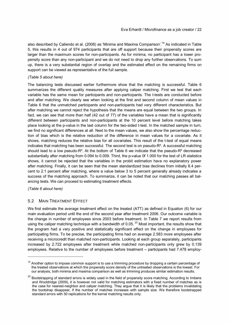
Eva Erhardt / Microfinance as a job creator / 22
also described by Caliendo et al. (2008) as ‘Minima and Maxima Comparison’.19 As indicated in Table 5, this results in 4 out of 974 participants that are off support because their propensity scores are larger than the maximum scores for non-participants. As for minima, no participant has a lower pro-pensity score than any non-participant and we do not need to drop any further observations. To sum up, there is a very substantial region of overlap and the estimated effect on the remaining firms on support can be viewed as representative of the full sample.
(Table 5 about here)
The balancing tests discussed earlier furthermore show that the matching is successful. Table 6 summarizes the different quality measures after applying caliper matching. First we test that each variable has the same mean for participants and non-participants. The t-tests are conducted before and after matching. We clearly see when looking at the first and second column of mean values in Table 6 that the unmatched participants and non-participants had very different characteristics. But after matching we cannot reject the hypothesis that the means are equal between the two groups. In fact, we can see that more than half (42 out of 77) of the variables have a mean that is significantly different between participants and non-participants at the 10 percent level before matching takes place looking at the p-value in the last column for the two-sided t-test. In the matched sample in turn, we find no significant differences at all. Next to the mean values, we also show the percentage reduc-tion of bias which is the relative reduction of the difference in mean values for a covariate. As it shows, matching reduces the relative bias for all covariates. This result of the t-test of equal means indicates that matching has been successful. The second test is on pseudo-R². A successful matching should lead to a low pseudo-R². At the bottom of Table 6 we indicate that the pseudo-R² decreased substantially after matching from 0.094 to 0.009. Third, the p-value 0f 1.000 for the test of LR statistics shows, it cannot be rejected that the variables in the probit estimation have no explanatory power after matching. Finally, it can be seen that the mean standardized bias declines from initially 8.4 per-cent to 2.1 percent after matching, where a value below 3 to 5 percent generally already indicates a success of the matching approach. To summarize, it can be noted that our matching passes all bal-ancing tests. We can proceed to estimating treatment effects.
(Table 6 about here)
5.2 MAIN TREATMENT EFFECT
We first estimate the average treatment effect on the treated (ATT) as defined in Equation (6) for our main evaluation period until the end of the second year after treatment 2006. Our outcome variable is the change in number of employees since 2003 before treatment. In Table 7 we report results from using the caliper matching technique with a bandwidth of 0.05. 20 Most important, the results show that the program had a very positive and statistically significant effect on the change in employees for participating firms. To be precise, the participating firms had on average 2.583 more employees after receiving a microcredit than matched non-participants. Looking at each group separately, participants increased by 2.722 employees after treatment while matched non-participants only grew by 0.139 employees. Relative to the number of employees before treatment – participants had 7.478 employ-
19 Another option to impose common support is to use a trimming procedure by dropping a certain percentage of
the treated observations at which the propensity score density of the untreated observations is the lowest. For our analysis, both minima and maxima comparison as well as trimming produces similar estimation results.
20 Bootstrapping of standard errors is widely used in the field of propensity score matching. According to Imbens and Wooldridge (2009), it is however not valid for matching estimators with a fixed number of matches as is the case for nearest-neighbor and caliper matching. They argue that it is likely that the problems invalidating the bootstrap disappear, if the number of matches increases with sample size. We therefore bootstrapped standard errors with 50 replications for the kernel matching results only.

Eva Erhardt / Microfinance as a job creator / 23
ees on average in 2003 – this translates into a growth difference in terms of firm size of 35 percent for participants compared to matched non-participants.
A look at the absolute number of employees before treatment in 2003 and after the main evaluation period in 2006 as indicated in the lower part of Table 7 complements the picture. First, it reveals that while the difference in firm size in 2003 was large between the two groups before matching (12.497 for unmatched non-participants), matching was successful in identifying a group of comparable non-participants with a similar firm size (7.478 for matched participants and 7.126 for matched non-participants). It secondly shows that the average Bulgarian firm in our dataset, that is the unmatched non-participants, even slightly shrank from 12.497 employees to 12.451 employees over the period 2003 to 2006. At the same time, microcredit participants grew from 7.478 to 10.200 employees, while the matched non-participants grew from 7.126 to 7.265. To sum up, microcredit considerably and significantly increased employment two years after treatment, while the average Bulgarian firm did not grow.
(Table 7 about here)
For comparison, we also indicate results for other matching algorithms in Table 8. As can be seen, the results from all matching estimators are significant and essentially give the same implications. The main ATT for change in employees until 2006 ranges from 2.438 employees based on nearest neigh-bor matching without replacement to 2.667 employees based on Kernel Matching with a bandwidth of 0.05 and a Gaussian weighting function. The closeness of results from different matching algorithms is not surprising according to Caliendo et al. (2008). With growing sample size all matching estimators become closer to comparing only exact matches and should yield the same results. Dehejia et al. (2002) even argue that the choice of matching algorithms is not as crucial as the proper estimation of the propensity scores. Still, finding similar results across different parameters serves as a robustness check and strengthens our confidence in the results.
(Table 8 about here)
5.3 DYNAMIC EFFECTS
While the previous results estimate the ATT for the main evaluation period until 2006, we now set the attention on analyzing the dynamic pattern of treatment effects. In other words, our interest is to dis-entangle the effect of the program to understand if it is constant or varies over time. We are able to do so, because information on the number of employees is available for several years after treatment. In addition, we can track firm exits in our dataset and hence control for sample attrition over a consider-able time span. Table 9 provides results of the estimated ATT for each year after treatment until 2010. It also shows the yearly development of absolute employee numbers for participants, matched non-participants and the full sample of non-participants which is in addition graphically illustrated in Figure 2. Since the number of observations varies slightly per year depending on the availability of infor-mation for sample firms in a certain year, we indicate it in the last two rows of Table 9. Note also that estimates are again very similar across different matching algorithms.
As Table 9 and Figure 2 show, the loan effects are substantially positive and long lasting as signifi-cant differences between the participating and matched non-participating firms are maintained several years after reception of the microcredit. A largely positive and statistically significant effect takes al-ready place in the treatment year 2004 with a difference of 2.760 more employees for microcredit participants. The strong program effect lessens towards the following year 2005 to a difference of 1.367 to recover again to 2.583 in 2006. Afterwards, the impact persist, but gradually decreases in terms of magnitude and significance. In 2010, the last available point in time in our dataset and six years after treatment the ATT still amounts to 1.913 with significance at the 5% level.

Eva Erhardt / Microfinance as a job creator / 24
What attracts attention is the remarkable dip in treatment effect for 2005. As can be seen in the sec-ond column of Table 9, the microcredit participants first grow strongly from a baseline size of 7.478 in 2003 to 10.286 employees until the end of the treatment year in 2004. Afterwards they contract to 8.790 employees in 2005 before recovering again to 10.200 in 2006. During the same time period, the matched and unmatched non-participants more or less stagnate at 7.071-7.265 employees and 12.07-12.497 employees respectively as shown in the third and fourth column of Table 9. The devel-opment of non-participants is in line with an economic context during that period which did not give reason for notable yearly changes. Moreover, the increase and subsequent drop in employees also does not mirror the underlying business fundamentals of participants. Financial indicators on sales, assets and profit for participants show a constant growth over the period 2003 to 2006.21 There exists no dip for financials in 2005 as it does for employee numbers. We thus suppose that the dramatic upward and downward development of firm size for microcredit participants is rather to be explained with the program itself. In anticipation or immediately after disbursement of the microcredit, participat-ing firms largely expanded their businesses in terms of employees within the year of treatment 2004. Presumably, this increase was oversized and unsustainable with regard to underlying business fun-damentals as financials did not increase at the same degree. This consequently triggered a clear contraction in terms of employees within the first year after treatment 2005, albeit the average firm size remained higher than before treatment. As the increase before, the decrease was again dispro-portional compared to financials and the average firm size for participants settles down at an apparent equilibrium of 10.200 employees in 2006. Another conjecture for the dip in 2005 would be that the expansion into new business areas as enabled by the microloan required a larger number of employ-ees in 2004 than one year later in 2005 when the new business processes had become more efficient and more experienced employees needed less time to perform the same tasks. Either way, it seems recommendable to consider an evaluation period of several years after treatment for microfinance programs in order to allow treatment effects on firm size to stabilize.
Another noticeable development that is mirrored in the dynamic treatment effects is the impact of the global economic crisis. If we look at the numbers of employees in Table 9, we see that after several years of growth the year 2009 marks a clear drop in firm size. Most plausibly, this reduction of em-ployees is to be explained by the economic downturn which followed the global financial crisis from 2007/2008. The crisis materialized very clearly in a downward movement of GDP and employment of the Bulgarian economy in the last quarter of 2008. GDP shrank by around 5 percent and unemploy-ment jumped in 2009. As studies for example by Wagner and Winkler (2013) show, microfinance insti-tutions have not been less vulnerable to the crisis than other financial institutions. While the crisis negatively affected both participants and non-participants, there exists however a difference in timing. Unmatched non-participants in our dataset start contracting in terms of firm size already one year earlier in 2008 than participants and matched non-participants. One conjecture for this earlier sensitiv-ity of the average Bulgarian firm to the economic shock is that microcredit clients and their matched comparators are more growth oriented firms and withstand economic pressures longer than other firms. Another reason for the time lag in decreasing firm sizes could also be related to origin of un-matched firms from sectors and locations which are less resistant to crises.
(Table 9 and Figure 2 about here)
21 For participants turnover gradually increases from 172 Thousand Euros (2003) to 193 TEUR (2004) to 234
TEUR (2005) to 295 TEUR (2006). Assets also increase from 125 TEUR (2003) to 206 TEUR (2004) to 303 TEUR (2005) to 532 TEUR (2006). Profit develops from 86 TEUR (2003) to 108 TEUR (2004) to 129 TEUR (2005) to 119 TEUR (2006). The exchange rates used in the Amadeus database come per default from the In-ternational Monetary Fund website and refer to the closing date of a month.

Eva Erhardt / Microfinance as a job creator / 25
5.4 HETEROGENEOUS EFFECTS In the following, we take a closer look on heterogeneity of the estimated treatment effect for different sub-groups. Specifically, we form various sub-groups of our main sample based on firm size, loan size, loan purpose and firm location. Then we re-estimate the ATT for each sub-group with propensity score matching. This way, we investigate for which sub-groups microcredit is in particular fostering growth. The results are summarized in Table 10. Note that we indicate at this stage both the ATT in terms of absolute change in the number of employees as well as the ATT in terms of relative change compared to the baseline number of employees. For certain sub-groups with very different average baseline numbers of employees, it is helpful to a have information on both.
5.4.1 FIRM SIZE
We first investigate whether the effect of microcredit varies with firm size. Our hypothesis according to evidence from other studies presented in section 2.2 is the following: the smaller a firm, the less it has access to formal bank loans. The more a firm is constrained by credit, the higher the relative impact of microcredit on its growth is supposed to be. We use the typical firm size categories micro (1-9 em-ployees), small (10-49) and medium (50-249). As a reminder, large firms with more than 250 employ-ees were eliminated from our sample during the data cleaning process. Next, we compare treatment effects between the different firm size categories. For this purpose, we look at the ATT for relative change in employees in the second column of Table 10, because average firm size naturally varies considerably between the three sub-groups. The results confirm our hypothesis. The smaller a firm, the higher the impact of microcredit on its growth in employees. Micro-sized firms have an ATT in relative terms of 24.7 percent more employees for participants than non-participants in 2006 com-pared to 2003. Small-sized participating firms increase by 22.0 percent more over the same time peri-od, while the treatment effect for medium-sized firms is insignificant with 1.1 percent increase.
5.4.2 LOAN SIZE
We also conduct the propensity score matching analysis for sub-groups of participants based on three different scales for loan amount: small (> 10,000 EUR), medium (10,000 – 50,000 EUR) and large (> 50,000 EUR). Since some participants received more than one loan during treatment, loan amounts reflect the total amount of all loans disbursed in 2004 per client. As can be seen in Table 10, the im-pact of all three size categories of microcredit is positive and significant (for large loan amounts at the 10%-level). Again, the average number of employees at baseline considerably varies, because loan size is proportionally linked to firm size. Larger firms need larger loan amounts. Hence, looking at the ATT in relative terms shows that the effect is very similar for small (33.7 percent) and medium (37.4 percent) loan amounts and additionally very similar to the base effect of microcredit for the full sample (34.5 percent). The ATT for large loan amounts of more than 50,000 EUR is slightly lower with an increase in employees of 24.7 percent for participants compared to baseline. One reason could be that small firms benefit more from microcredit as demonstrated above and that larger loans are grant-ed to larger firms which benefit less, because they find it easier than small firms to access bank loans.
5.4.3 LOAN PURPOSES
Another analysis based on features of the loan is performed for different loan purposes. The bank distinguishes between loans for working capital and investment. Working capital refers to current or short-term assets to be used within one year. Working capital loans are therefore for current expendi-tures that occur in the normal course of business. Examples comprise wood purchased for carpentry or food and goods for retail vending. Investment loans are those made for the purchase of fixed as-sets that are used over time of the business. These assets typically have a life span of more than one

Eva Erhardt / Microfinance as a job creator / 26
year such as machinery, equipment or property. Examples of investments for small businesses would include sewing machines for tailors, refrigerators for retail businesses or a tractor for an agricultural business. A loan made for the investment in fixed assets is generally for a larger amount and for a longer term than a working capital loan. Since the productive activity does not directly use up the fixed asset (that is, not sold as part of the product), economic theory suggests that the impact of investment loans upon profitability (and business expansion in terms of employees) is felt over a longer period of time (Ledgerwood, 2013). The impact of working capital loans on the other hand is supposed to show instantaneously and diminish over time. Our dataset largely supports this hypothesis. We estimate an impact in 2006 of 2.879 for working capital loans and 1.679 for investment loans as shown in Table 10. A shorter-term perspective further illustrates the more immediate impact of working capital over investment loans. Whereas working capital loans have an ATT of 3.114 in 2004 (1.377 in 2005), in-vestment loans have an ATT of only 2.449 in 2004 (1.121 in 2005). From 2008 onwards, the relation-ship in terms of impact from working capital loans to investment loans reverses and investment loans have a higher impact than working capital loans (3.635 in 2008, 3.941 in 2009 and 2.875 in 2010 for investment loans compared to 2.858 in 2008, 2.174 in 2009 and 2.062 in 2010 for working capital loans). All of the indicated ATTs are significant. While it needs to be questioned for how long after treatment in general an impact can be attributed to the original microloan, the findings point into the direction that the period over which loans display their impact is affected by the loan purpose. It seems therefore advisable to take the type of loan purpose into consideration when deciding over the appropriate evaluation period for microfinance impact assessments. In addition, our findings do not add support to the frequently made caveat that because money is fungible (e. g. Banerjee et al., 2013; Ledgerwood, 2013) loans intended for a specific purpose are often used for a different purpose within a household or business.
5.4.4 LOCATION
Finally, we make use of the fact that the microcredit program was not present in all Bulgarian districts at treatment. As Figure 1 shows, ProCredit Bank Bulgaria had branches in 19 out of 28 Bulgarian districts during treatment in 2004. Observations for non-participants are available for all of the 28 dis-tricts. We now exploit this institutional feature of the program by including only firms from the 9 dis-tricts without program presence as potential comparators in the matching regressions. It should be noted that we had to drop a small amount of 28 from 974 participants which were located in districts without actual presence of the program, but still participated. Overall, propensity score matching re-sults again in a significant positive ATT of an increase in employees of 2.421 more for participants than for non-participants from districts without the program. The fact that the ATT is very similar to our main estimation when matching only on a sample of non-participants from areas without the program, is an important finding for the applicability of our research design. For areas without program pres-ence, we have good reason to believe that access to alternative credit (a concern addressed in sec-tion 2.2) was in general much more limited than in program areas. It is the case, because ProCredit Bank followed a typical strategy for financial institutions by focusing on economically more developed areas first. Hence it is very likely that not only Pro Credit Bank Bulgaria, but also other providers of microcredit had limited presence in areas without the program. Receiving still a very similar ATT of 2.412 to the ATT of 2.583 from our main estimation then supports our hypothesis that in general little alternative credit was available for non-participants both in program and non-program areas.
(Table 10 about here)
To sum up, the purpose of this section was to investigate for which sub-groups of our sample micro-credit is particularly enhancing growth. We find that the treatment effect increases with decreasing firm size and is largest for micro-enterprises. This adds further evidence to other studies which find that smaller firms are more constrained by credit than are larger firms. Since loan sizes are also linked

Eva Erhardt / Microfinance as a job creator / 27
to underlying firm size, we find a similar inverse relationship. The impact of microcredit decreases with increasing loan amounts. In addition, our findings point to the fact that the period over which loans display their impact is affected by the loan purpose. Working capital loans show a more immediate effect, while loans for investment purposes increase their impact over time. Finally, we are able to show that restricting the sample of non-participants to areas without program presence results in simi-lar treatment effects than from our main estimation. This finding supports our hypothesis that alterna-tive credit to non-participants was still limited during the period of evaluation and raises confidence in our research design.
6 SENSITIVITY TESTS After having presented strong positive effects of the program, we test the robustness of our results. First, we try to verify that the model specification is appropriate and results are robust to variations within the matching process. Then, we check the key assumptions of the estimation and that results do not suffer from bias.
The advantage of well-performed matching is that it can account for selection on observables as dis-cussed in section 4. In this regard, some typical sources of bias in non-experimental studies can be ruled out. Matching effectively reweights data for non-participants to equate the distribution of observ-able attributes between participants and non-participants and it requires common support. This means that if participation in microcredit can be understood with observable variables, then matching produces consistent results. To add further strength to our estimates in this regard, we will test their sensitivity to small changes in the specification of the propensity score estimation. In addition, we will compare our main results with propensity score matching (PSM) to treatment effects estimated through a linear regression model with ordinary least squares (OLS).
Even if selection on observables is well accounted for, one major drawback of matching in contrast to randomized experiments remains nevertheless: selection on unobservables is not controlled for. By complementing propensity score matching with difference-in-differences, we try to control for any pre-existing constant (time-invariant) differences in the outcome variable before treatment, even if those differences are caused by unobservable attributes. Still, participants and non-participants could differ in terms of time-variant unobserved characteristics. This would violate the conditional independence assumption and bias our results. It is not possible to directly test the conditional independence as-sumption and the magnitude of selection bias with our non-experimental data. We can however as-sess the sensitivity of our results to remaining unobservables and will do so by applying the so-called bounding and simulation analyses.
6.1 VARIATIONS WITHIN MATCHING PROCESS To start with, an initial robustness check in terms of variation within the matching process was already built in our presentation of main results. We jointly considered different matching methods in Table 8. The fact that matching with different methods such as caliper, nearest neighbor, radius and kernel estimators produces very similar results, is a positive sign for robustness. Now, we additionally extend the set of variables in the propensity score estimation in order to see whether this has an impact on the causal estimates as for example suggested by Dehejia et al. (2002).
As explained above, it is a major limitation of the dataset that data availability for financials such as sales, profit and assets as well as historical trends before start of the treatment in 2003 are only avail-able for a limited amount of firms in our sample. We consequently restricted our main specification to variables which allow for a large sample size. Now, we make use of the additional information availa-ble for a reduced sample. First, we add information on more years prior to treatment for estimating the

Eva Erhardt / Microfinance as a job creator / 28
propensity score than we did for our base estimation of the ATT. The point of reference is the base ATT for change in employees until 2006 of 2.538 as shown in the first row of Table 11. If we now in-clude information on employees, sales, profit, assets and profitability for 2002 in our propensity score estimation, we get an even higher and still significant (10% level) effect of 4.243. Sample size reduces to 140 matched participants and 13,454 matched non-participants (from 970 and 57,691 respectively for base effects). Going further backwards in time, so as to match on longer trends before start of the treatment, produces the following results: We add information on the number of employees for 2002, 2001 and 2000, that is until 3 years before start of the treatment to our base specification. The esti-mated program effect increases to 3.201 compared to baseline results with significance at the 1% level. If we instead use the change in employee numbers from 2003 compared to 2000 as further variable for the matching process, this results in an significant ATT of 2.405.
Furthermore, we assess how the inclusion of additional variables for the baseline year 2003 influ-ences results. If we use information on both sales and profit in 2003 for propensity score matching, the impact increases to 3.011. Including assets or productivity as further variables, leads to insignifi-cant results.
Finally, we modify the specification of the propensity score estimation with regard to geographic loca-tion. As Heckman et al. (1997) show, geographical mismatch of participants and non-participants is typically a large source of bias in impact studies. As a consequence, we here exactly match on dis-trict. In detail, we only include matches of participants and non-participants if they are exactly identical in terms of district. It should be noted that we already use districts as covariate for the estimation of propensity scores in our main sample. Consequently, many matches used for estimating the base effect already fulfill this condition. If we now explicitly force an exact match on location by district, the effect amounts to a significant increase of 1.850 more employees in 2006 for participants compared to 2003 before treatment which is about in the same range as the base effect of 2.583 as can be seen in Table 11.
(Table 11 about here)
The first point we can make here is that the inclusion of longer time trends for certain variables as well as the extension of the set of variables for the baseline year 2003 in the matching process largely confirms the positive and significant effect of microcredit. The consideration of longer time trends be-fore treatment provides yet a further important insight: it allows us to graphically show for a sub-sample that participants and matched non-participants developed almost identically in terms of firm size for several years before the treatment of participants with microcredit. After treatment, only partic-ipants start to grow considerably while matched non-participants stagnate. This strongly supports our hypothesis that the increase in firm size for participants compared to otherwise identical matched non-participants (based on observable characteristics) is causally related to treatment with microcredit. Figure 3 graphically illustrates this fact for the period 2000 until 2006 based on an extension of the specification for propensity score estimation by the change in employee numbers from 2003 com-pared to 2000 (Δ N employees 2003 – N employees 2000). The sub-sample consists of 331 partici-pants and 34,052 non-participants. The finding that participants and their matched non-participants had a very similar development of firm size before treatment finally also relates to the applied differ-ence-in-differences method. It adds support to our assumption that in absence of the program both participants and non-participants would have the same trend in the outcome variable.
(Figure 3 about here)

Eva Erhardt / Microfinance as a job creator / 29
6.2 OLS ESTIMATES As another robustness test, we compare our main results with propensity score matching (PSM) to treatment effects estimated through a linear regression model with ordinary least squares (OLS). Both methods are supposed to produce similar result, although PSM has two particular advantages com-pared to OLS according to Chemin (2008). First, matching compares a participant to a synthetic non-participant only if the synthetic non-participant is comparable enough to the participant, that is in the area of common support. On the other hand, a regression with OLS will give a result by interpolating a linear relationship between the two groups, no matter if participants and non-participants are very different. This is an undesirable result if the two groups are not comparable. Second, the matching technique is non-parametric as opposed to a linear regression imposing a linear structure on the data. After a synthetic non-participant is built, outcomes between the participant and the synthetic non-participant are differenced. Unlike for OLS, no particular structure is imposed on the data and hetero-geneous treatment effects are allowed for.
Table 12 summarizes the OLS estimates for different models and compares them to results from PSM. We first estimate a model without control variables both according to PSM and OLS, i. e. with only a constant and the treatment variable. It does not take into account any observable difference between participants and non-participants. In contrast, the estimated treatment effect for the second model with control variables includes all covariates in OLS which were also used for estimating the propensity score. In addition, we performed the OLS estimation for two types of samples. We first used the full sample with all available non-participants (61,006 observations) and then the reduced sample with only the non-participants, that were used for matching (58,665 observations). The full sample uses more information, whereas the reduced sample should provide a better approximation of the ATT with PSM, because it is applied to the same sample.
(Table 12 about here)
The results for change in employees until 2006 before matching in the first column of Table 12 are very similar for propensity score matching and for OLS without control variables as expected. If we look at the matched sample only, the estimates for unmatched PSM and OLS are identical with a change of 2.771 in employees, because no observable differences between participants and non-participants are accounted for. When we compare our main results from PSM after matching to the OLS estimates with the control variables in the second column, we receive a lower, but still consider-able and significant ATT for OLS on the matched sample of 1.841. Overall, the fact that an estimation with OLS results in a similar positive and significant effect of microcredit on the change in employees from 2003 to 2006 further points to the robustness of our results from propensity score matching.
6.3 BOUNDING AND SIMULATION ANALYSIS In order to assess how strong an unobserved component would need to be so as to undermine our results, we ultimately apply bounding and simulation analysis as used by Caliendo and Künn (2011).
The so-called bounding approach was initially suggested by Rosenbaum (2002) who describes the main ideas as follows: The bounding approach introduces a sensitivity parameter Γ that measures the degree of departure from random assignment of treatment. Two subjects with the same observed covariates may differ in their odds of receiving the treatment by at most a factor of Γ (≥ 1). In an ex-periment, random assignment of treatment ensures that Γ = 1, so no sensitivity analysis is needed. In an observational study with for example Γ =2 if two subjects were matched exactly for observed co-variates, then one might be twice as likely as the other to receive the treatment because they differ in terms of a covariate not observed. Of course, in an observational study Γ is unknown. Bounding tries out several values of Γ to see how the conclusions might change. For each value of Γ, it is possible to place bounds on a statistical inference. We implement the bounding approach by using the rbounds

Eva Erhardt / Microfinance as a job creator / 30
procedure in Stata which was developed by DiPrete and Gangl (2004) for continuous outcome varia-bles. rbounds uses the results from the matching estimates to calculate maximum and minimum p-values from a Wilcoxon's signed rank test between matched pairs of participating and non-participating firms for an artificial unobserved variable with different values of Γ. The p-values then represent the bound on the significance level of the treatment effect in the case of endogenous selec-tion into treatment. We compare the Rosenbaum bounds on treatment effects at different levels of Γ. This way, we can assess the strength that such unobserved influences must have so that the esti-mated treatment effects from propensity score matching would have arisen purely through non-random assignment.
It is important to recognize that the results from the Rosenbaum bounds are a ‘‘worst-case’’ scenario. DiPrete et al. (2004) provide an example where p-values become significant at Γ = 1.15 and point to the fact that such a result does not mean that there is no positive effect of treatment on outcome. It rather means that the confidence interval for the effect would include zero if an unobserved variable caused the odds ratio of treatment assignment to differ between participants and non-participants by 1.15 and if this variable’s effect on outcome was so strong as to almost perfectly determine whether the outcome would be bigger for the participants or the non-participants in each pair of matched cas-es in the data. In the case where a unobserved variable had an equally strong effect on selection into treatment but only a weak effect on the outcome variable, the confidence interval for employment would not contain zero. Nonetheless, the Rosenbaum bounds convey important information about the level of uncertainty contained in matching estimators by showing just how large the influence of an unobserved variable must be to undermine the conclusions of a matching analysis.
(Table 13 about here)
Table 13 summarizes the results of the bounding analysis. If unobserved factors lead to negative or positive selection, i. e. those who participate always have a lower or higher growth rate of employees than matched non-participants even in the absence of treatment, the p-values will become significant for a certain value of Γ. In the absence of unobserved heterogeneity, that is Γ =1.00, the p-values are insignificant indicated by a p < 0.05. Starting from that point, we stepwise increase the value of Γ and simulate an ascending influence of unobserved factors. At Γ =2.00 the range of possible p-values is from 0.000 to 0.001, so a bias of this magnitude could not explain the larger firm size increase for participants. If we had failed to control by matching a variable strongly related to firm growth and two times more common among participants, this would not have been likely to produce a difference in employee growth as large as the one we observe (see Rosenbaum, 2002 for a similar example). The upper bound of the p-value becomes finally significant at the 5% level when Γ = 2.30. Two firms that have the same observable characteristics would then differ in their odds of participating in the micro-credit program by a factor of 2.30 or 130 percent. In other words, unobserved factors would need to have about one and a third times the influence as observed factors in order to undermine the results. This can be considered to be a reasonably large number given that we have adjusted for many im-portant observed factors (see for example Aakvik, 2001 or Caliendo et al., 2011). Consequently, we conclude that our results on the change in employees are robust against strong unobserved selection bias. Put in another way, the influence of a an unobserved factor would have to be considerable to undermine the conclusions of our matching analysis.
Since the critical values from bounding are rather abstract, we additionally implement the so-called simulation analysis to better illustrate the magnitude of potential hidden bias which would cause us to revise our findings of causal effects of microfinance on employment levels. Simulation analysis was originally applied as sensitivity test to matching by Ichino et al. (2008). Its basic idea is to start from the conditional independence assumption and then examine how the results change as this assump-tion is weakened in specific ways, whereas for the bounding analysis the conditional independence assumption was entirely dropped. We perform the analysis by simulating an unobserved variable or

Eva Erhardt / Microfinance as a job creator / 31
so-called confounder that is adapted to the distribution of an observable variable. Since we exactly know the influence of the observable characteristics on outcomes and selection, we therefore have a direct linkage to the potential unobserved effect for the interpretation. Results are shown in Table 14.
(Table 14 about here)
The first two columns in Table 14 show the influence of each confounder on the untreated outcome and on the selection into treatment. Thereby, a value below (above) 1 indicates a negative (positive) impact. The third column shows the resulting ATT given the existence of a confounder with a certain distribution. The last column contains the standard error of the ATT. To facilitate a comparison be-tween actual and simulated results, the first row of Table 14 shows the baseline ATT estimate ob-tained with no confounder in the matching set. In the absence of a confounder, its influence on out-come and selection is obviously zero and the ATT is 2.422 from nearest-neighbor matching. The fol-lowing rows of Table 14 show how the baseline estimate changes when the confounding factor is calibrated to mimic different observable covariates and is then included in the set of matching varia-bles. If a confounder is introduced which has the identical distribution as the firm size ‘small’, the influ-ence on outcome (0.593) and on selection (0.871) would be negative. This means that such an unob-served term would have a negative effect on the change in employees in case of no treatment and also on being treated at all. Including this simulated unobserved confounder leads to an ATT of 1.895 which is within the range of the ATT in the absence of unobserved heterogeneity. We tested other confounders as well. A confounder with the distribution of ‘Ownership type (Joint Stock Company)’ would lead to an ATT of 1.883. The simulation of a confounder with a distribution of ‘Gender of owner (female)’ finally results in an ATT of 1.824. Taken in conjunction, these simulations result in ATTs which are of a similar dimension as the baseline ATT. This means that the existence of any unob-servables which influence selection or outcome by a similar magnitude as certain observable varia-bles, would still not largely alter the positive effect of the microfinance program on creating jobs for participating firms.
To repeat, no test can directly justify the unconfoundedness assumption. However, the performed bounding and simulation analyses convey an impression of robustness of the baseline matching esti-mates of the ATT. Overall, the presented sensitivity analyses find that the direction and dimension of our estimated treatment effect holds which increases confidence in the robustness of our results even with respect to unobserved heterogeneity.
7 CONCLUSIONS In this paper, we analyze the impact of a microfinance program for small firms in Bulgaria. The pro-gram is intended to ease credit constraints of small firms and thus contribute to job creation in partici-pating firms. The unique firm-level panel data used, provides an important opportunity to address two research gaps in the previous literature on microfinance impact assessments at the same time: First of all, we are able to add to the scarce literature on wage-employment effects of microfinance beyond measuring self-employment or employment of family members as most other assessments are limited to. Second, by providing evidence for relatively large, individual loans from a microfinance bank in Bulgaria, this study also contributes to the largely neglected area on impact of microfinance in the transition economies of Eastern Europe and Central Asia.
We base our analysis on propensity score matching and extend the standard approach to a differ-ence-in-differences matching estimator to assess the effectiveness of participating in the microcredit program against non-participation. Our identifying assumption is that conditional on the information in our dataset, selection into the program can be assumed to be random such that differences in out-come between participants and non-participants can be interpreted as causal effects. We find a rela-tively large positive and significant effect of microcredit on employment. We find evidence that pro-

Eva Erhardt / Microfinance as a job creator / 32
gram participation is indeed causally related to an increase in the number of employees. Participating firms have on average 2.6 more employees two years after receiving a microcredit than matched non-participants. Related to the number of employees before treatment, this translates into a growth dif-ference in terms of firm size of 35 percent for participants. The microcredit program also has a long lasting impact on job creation. Significant differences between the participating and matched non-participating firms exist for as long as at least six years after reception of the microcredit. At the same time, the increase in the number of employees for participants is characterized by initial upward and downward adjustments during the first two years after treatment before stabilizing at the new, higher level of firm size. Consequently, only an evaluation period of several years after treatment seems able to capture the sustainable impact of microfinance on firm growth. Heterogeneous effects for sub-groups support the finding from other studies that smaller firms are more constrained by credit than are larger firms. In fact, the treatment effect increases with decreasing firm size and is largest for mi-cro-enterprises. In addition, our results from sub-analyses of effects based on loan purposes point to the fact that the time at which the impact occurs is affected by the loan purpose. While working capital loans show a more immediate effect, loans for investment purposes increase their impact over time. It seems therefore advisable to take the type of loan purpose into consideration when deciding over the appropriate evaluation period for microfinance impact assessments.
Since selection bias is always an issue for evaluations as participating firms have observed and un-observed characteristics that make them different from other firms, we carefully assess the sensitivity of our results. We do so in several ways. First we assess the robustness of our results to small changes in the matching process. We show for a reduced sample that the extension of the set of vari-ables for our baseline year as well as the inclusion of longer time trends does not have an impact on the causal estimates. Neither does the application of different matching estimators. In fact, the con-sideration of longer time trends before treatment additionally reveals that in absence of the program both participants and non-participants would have the same trend in the outcome variable. Then, we compare our main results with propensity score matching to treatment effects estimated through a linear regression model with ordinary least squares. Results from both methods are similar. At last, we apply so-called bounding and simulation analyses in order to examine how strong any remaining un-observed differences would need to be in order to undermine the results. It turns out that results are again robust. The bounding approach shows that unobserved factors would need to be considerably large in order to undermine the results. Precisely, unobservables would need to have about 1.3 times the influence on selection and outcome as the observed variables used for our estimation. In the same manner, the simulation of confounding variables based on observable covariates leads to simi-lar results as our base effects. This means that the existence of any unobservables which influence selection or outcome by a similar magnitude as certain observable variables, would still not largely alter the positive effect of the microfinance program on creating jobs for participating firms.
Finally, an issue that is neglected in this paper is the analysis of not only benefits but also costs of delivering microcredit. We know that the microfinance bank which provided the program loans is sus-tainably operating. A complete evaluation of the cost-effectiveness would require however a detailed estimation of the program’s direct and administrative costs as well as of valuing the gains in employ-ment in participating firms in monetary terms. This is beyond the scope of this study and could be the subject of future research. Another avenue for further research are crowding-out effects of firm growth. While we find positive effects of microcredit on the growth of participating firms, they might prosper at the expense of non-participating firms in their sector or location. As a result, the net em-ployment effect at the firm level would be offset at the aggregate level if firm growth within a sector or location is a zero-sum game.

Eva Erhardt / Microfinance as a job creator / 33
8 REFERENCES Aakvik, A. (2001). Bounding a matching estimator: the case of a Norwegian training program. Oxford
Bulletin of Economics and Statistics, 63 (1), 115-143. Abou-Ali, H., El-Azony, H., El-Laithy, H., Haughton, J., & Khandker, S. (2010). Evaluating the impact
of Egyptian Social Fund for Development Programs. cJournal of Development Effectiveness, 2 (4), 521-555.
Angelucci, M., Karlan, D., & Zinman, J. (2015). Microcredit impacts: Evidence from a randomized microcredit program placement experiment by Compartamos Banco. American Economic Journal: Applied Economics, 7 (1), 151-182.
Armendáriz de Aghion, B., & Morduch, J. (2000). Microfinance beyond group lending. Economics of Transition, 8 (2), 401-420.
Armendáriz de Aghion, B., & Morduch, J. (2010). The Economics of Microfinance. Cambridge, Massachusetts: MIT Press.
Attanasio, O., Augsburg, B., De Haas, R., Fitzsimons, E., & Harmgart, H. (2011). Group lending or individual lending? Evidence from a randomised field experiment in Mongolia. EBRD Working Paper, 136.
Augsburg, B., De Haas, R., Harmgart, H., & Meghir, C. (2012). Microfinance at the margin: experimental evidence from Bosnia and Herzegovina. EBRD Working Paper, 146.
Ayyagari, M., DemirgC, & Maksimovic, V. (2010). Formal versus informal finance: Evidence from China. Review of Financial Studies, 23 (8), 3048-3097.
Ayyagari, M., Demirgüç-Kunt, A., & Maksimovic, V. (2008). How important are financing constraints? The role of finance in the business environment. The World Bank Economic Review, 22 (3), 483-516.
Bah, E.-h., Brada, J., & Yigit, T. (2011). With a little help from our friends: The effect of USAID assistance on SME growth in a transition economy. Journal of Comparative Economics, 39 (2), 205-220.
Banerjee, A., Duflo, E., Glennerster, R., & Kinnan, C. (2013). The miracle of microfinance? Evidence from a randomized evaluation. MIT Department of Economics Working Paper, 13-09.
Banerjee, A., Karlan, D., & Zinman, J. (2015). Six randomized evaluations of microcredit: introduction and further steps. American Economic Journal: Applied Economics, 7 (1), 1-21.
Beck, T., Demirgüç-Kunt, A., Laeven, L., & Maksimovic, V. (2006). The determinants of financing obstacles. Journal of International Money and Finance, 25 (6), 932-952.
Beck, T., Demirgüç-Kunt, A., & Maksimovic, V. (2005). Financial and Legal Constraints to Growth: Does Firm Size Matter? Journal of Finance, 60 (1), 137-177.
Beck, T., Demirgüç-Kunt, A., & Maksimovic, V. (2008). Financing patterns around the world: Are small firms different? Journal of Financial Economics, 89 (3), 467-487.
Becker, S., & Ichino, A. (2002). Estimation of average treatment effects based on propensity scores. Stata Journal, 2 (4), 358–377.
Binswanger, H. P., & Khandker, S. R. (1995). The impact of formal finance on the rural economy of India. Journal of Development Studies, 32 (2), 234-262.
Brown, J. D., & Earle, J. S. (2010). Firm-level growth effects of small loan programs: estimates using universal panel data from Romania. mimeo.
Bruhn, M., & Love, I. (2009). The economic impact of banking the unbanked: evidence from Mexico. World Bank Policy Research Working Paper, 4981.
BSMEPA, & CED. (2004). Report about SMEs, 2002-2003 Sofia: Bulgarian Small and Medium Enterprises Promotion Agency.
BSMEPA, & NOEMA. (2011). Analysis of the situation and factors for development of SMEs. Sofia: Bulgarian Small and Medium Enterprises Promotion Agency.
Budina, N., Garretsen, H., & De Jong, E. (2000). Liquidity Constraints and Investment in Transition Economies. Economics of Transition, 8 (2), 453-475.
Burgess, R., & Pande, R. (2005). Do rural banks matter? Evidence from the Indian social banking experiment. American Economic Review, 95 (3), 780-795.
Caliendo, M., & Kopeinig, S. (2008). Some practical guidance for the implementation of propensity score matching. Journal of Economic Surveys, 22 (1), 31-72.
Caliendo, M., & Künn, S. (2011). Start-up subsidies for the unemployed: Long-term evidence and effect heterogeneity. Journal of Public Economics, 95 (3-4), 311-331.

Eva Erhardt / Microfinance as a job creator / 34
Cameron, A. C., & Trivedi, P. K. (2005). Microeconomics: methods and applications. Cambridge: Cambridge University Press.
Caudill, S. B., Gropper, D. M., & Hartarska, V. (2009). Which microfinance institutions are becoming more cost effective with time? Evidence from a mixture model. Journal of Money, Credit and Banking, 41 (4), 651-672.
CGAP. (2015). Spotlight on International Funders’ Commitments to Financial Inclusion. CCAP Brief March 2015. Washington, DC: CGAP.
Chemin, M. (2008). The Benefits and Costs of Microfinance: Evidence from Bangladesh. Journal of Development Studies, 44 (4), 463-484.
Coad, A., & Hölzl, W. (2010). Firm growth: Empirical analysis. Papers on economics and evolution, 1002.
Coleman, B. E. (1999). The impact of group lending in Northeast Thailand. Journal of Development Economics, 60 (1), 105-141.
Coleman, B. E. (2006). Microfinance in Northeast Thailand: Who benefits and how much? World Development, 34 (9), 1612-1638.
Crépon, B., Devoto, F., Duflo, E., & Pariente, W. (2014). Estimating the impact of microcredit on those who take it up: Evidence from a randomized gexperiment in Morocco. NBER Working Paper, 20144.
Cull, R., Demirguc-Kunt, A., & Morduch, J. (2009). Microfinance Meets the Market. Journal of Economic Perspectives, 23 (1), 167-192.
de Kok, J., Vroonhof, P., Verhoeven, W., Timmermans, N., Kwaak, T., Snijders, J., & Westhof, F. (2011). Do SMEs create more and better jobs? Zoetermeer, The Netherlands: EIM Business & Policy Research.
De Mel, S., McKenzie, D., & Woodruff, C. (2008). Returns to capital in microenterprises: evidence from a field experiment. Quarterly Journal of Economics, 123 (4), 1329-1372.
Dehejia, R. H., & Wahba, S. (2002). Propensity score-matching methods for nonexperimental causal studies. Review of Economics and Statistics, 84 (1), 151-161.
DiPrete, T. A., & Gangl, M. (2004). Assessing bias in the estimation of causal effects: Rosenbaum bounds on matching estimators and instrumental variables estimation with imperfect instruments. Sociological methodology, 34 (1), 271-310.
Duenwald, C. K., Gueorguiev, N., & Schaechter, A. (2005). Too much of a good thing? Credit booms in transition economies: The cases of Bulgaria, Romania, and Ukraine. lIMF Working Paper, 05/128.
Dunn, E., & Arbuckle, J. G. (2001). Microcredit and microenterprise performance: impact evidence from Peru. Small Enterprise Development, 12 (4), 22-33.
Duval, A., & Goodwin-Groen, R. (2005). Experienced Consortium Deepens Bulgarian Financial System by Creating ProCredit Bank, a Commercial Bank for Microenterprises. CGAP Case Studies in Donor Good Practices, 20.
Duvendack, M., & Palmer-Jones, R. (2012). High noon for microfinance impact evaluations: re-investigating the evidence from Bangladesh. Journal of Development Studies, 48 (12), 1864-1880.
Duvendack, M., Palmer-Jones, R., Copestake, J. G., Hooper, L., Loke, Y., & Rao, N. (2011). What is the evidence of the impact of microfinance on the well-being of poor people? London: EPPI-Centre, Social Science Research Unit, Institute of Education, University of London.
EU. (2005). The New SME Definition: User Guide and Model Declaration. Enterprise and Industry Publications. Brussels: European Commission.
EU. (2008). SBA Fact Sheet 2008: Bulgaria. Enterprise and Industry Publications. Brussels: European Commission.
European-Union. (2010). Europe 2020: A Strategy for Smart, Sustainable and Inclusive Growth - Communication from the Commission: Publications Office of the European Union.
Fisher, R. A. (1937). The design of experiments. Edingburgh: Oliver and Boyd. Grimm, M., & Paffhausen, A. L. (2015). Do interventions targeted at micro-entrepreneurs and small
and medium-sized firms create jobs? A systematic review of the evidence for low and middle income countries. Labour Economics, 32, 67-85.
Gubert, F., & Roubaud, F. (2011). The Impact of Micro Finance Loans on Small Informal Enterprises in Madagascar. A Panel Data Analysis. Social Protection Series. The World Bank, No. 77931.

Eva Erhardt / Microfinance as a job creator / 35
Guirkinger, C. (2008). Understanding the coexistence of formal and informal credit markets in Piura, Peru. World Development, 36 (8), 1436-1452.
Hartarska, V., Caudill, S. B., & Gropper, D. M. (2006). The cost structure of microfinance institutions in eastern Europe and central Asia. William Davidson Institute Working Paper No. 809.
Hartarska, V., & Nadolnyak, D. (2008). An Impact Analysis of Microfinance in Bosnia and Herzegovina. World Development, 36 (12), 2605-2619.
Heckman, J. J., Ichimura, H., & Todd, P. E. (1997). Matching as an econometric evaluation estimator: Evidence from evaluating a job training programme. Review of economic studies, 64 (4), 605-654.
Hutchinson, J., & Xavier, A. (2006). Comparing the impact of credit constraints on the growth of SMEs in a transition country with an established market economy. Small Business Economics, 27 (2-3), 169-179.
Ichino, A., Mealli, F., & Nannicini, T. (2008). From temporary help jobs to permanent employment: What can we learn from matching estimators and their sensitivity? Journal of Applied Econometrics, 23 (3), 305-327.
Imbens, G. W. (2004). Nonparametric estimation of average treatment effects under exogeneity: A review. Review of Economics and Statistics, 86 (1), 4-29.
Imbens, G. W., & Wooldridge, J. M. (2009). Recent developments in the econometrics of program evaluation. Journal of Economic Literature, XLVII (March 2009).
Karlan, D., & Morduch, J. (2010). Access to Finance. In D. Rodrik & M. Rosenzweig (Eds.), Handbook of Development Economics (Vol. 5, pp. 4703 – 4784.): Elsevier.
Karlan, D., & Zinman, J. (2011). Microcredit in Theory and Practice: Using Randomized Credit Scoring for Impact Evaluation. Science, 332 (6035), 1278-1284.
Ledgerwood, J. (2013). Microfinance new handbook: a financial market system perspective. Washington: The Worldbank.
Leuven, E., & Sianesi, B. (2003, Version 4.0.10). PSMATCH2: Stata module to perform full Mahalanobis and propensity score matching, common support graphing, and covariate imbalance testing. Retrieved on January 20th, 2014.
Maes, J. P., & Reed, L. R. (2012). State of the microcredit summit campaign report 2012. Washington D.C: Microcredit Summit Campaign.
McKenzie, D., & Woodruff, C. (2008). Experimental evidence on returns to capital and access to finance in Mexico. The World Bank Economic Review, 22 (3), 457-482.
Ministry of Economy. (2004). Annual report on the condition and development of SMEs in Bulgaria 2004. Sofia: Ministry of Economy, Energy, Tourism.
MIX-Market. (2013). Convergences Microfinance Barometer 2013. Retrieved April 13 2016 http://www.convergences.org/en/bibliotheque/microfinance-barometer-2013/
Montgomery, H. (2005). Meeting the Double Bottom Line: The Impact of Khushali Bank's Microfinance Program in Pakistan. Asian Development Bank Policy Papers, 8.
Nannicini, T. (2007). Simulation-based sensitivity analysis for matching estimators. Stata Journal, 7 (3), 334.
Neyman, J. (1923, 1990). On the application of probability theory to agricultural experiments. Essay on principles. Section 9, translated and edited by D.M Dabrowska and T.P. Speed. Statistical Science, 5 (4), 465-472.
Pande, R., Cole, S., Sivasankaran, A., Bastian, G. G., & Durlacher, K. (2012). Does poor people’s access to formal banking services raise their incomes? : EPPI-Centre, Social Science Research Unit, Institute of Education, University of London.
Pissarides, F., Singer, M., & Svejnar, J. (2003). Objectives and constraints of entrepreneurs: evidence from small and medium size enterprises in Russia and Bulgaria. Journal of Comparative Economics, 31 (2003) 503–531.
Pitt, M., & Khandker, S. (1998). The Impact of Group-Based Credit Programs on Poor Households in Bangladesh: Does the Gender of Participants Matter? Journal of Political Economy, 106 (5), 958-996.
Rosenbaum, P. R. (2002). Observational study. Encyclopedia of Statistics in Behavioral Science, 3, 1451-1462.
Rosenbaum, P. R., & Rubin, D. B. (1983). The central role of the propensity score in observational studies for causal effects. Biometrika, 70 (1), 41-55.

Eva Erhardt / Microfinance as a job creator / 36
Rosenbaum, P. R., & Rubin, D. B. (1985). Constructing a control group using multivariate matched sampling methods that incorporate the propensity score. The American Statistician, 39 (1), 33-38.
Roy, A. D. (1951). Some thoughts on the distribution of earnings. Oxford Economic Papers, 3 (2), 135-146.
Rubin, D. B. (1974). Estimating causal effects of treatments in randomized and nonrandomized studies. Journal of Educational Psychology, 66 (5), 688.
Rubin, D. B., & Thomas, N. (1996). Matching using estimated propensity scores: relating theory to practice. Biometrics, 249-264.
Setboonsarng, S., & Parpiev, Z. (2008). Microfinance and the Millennium Development Goals in Pakistan: Impact assessment using propensity score matching. ADB Institute Discussion Papers, 104.
Smith, J. A., & Todd, P. E. (2005). Does matching overcome LaLonde's critique of nonexperimental estimators? Journal of Econometrics, 125 (1), 305-353.
Stewart, R., van Rooyen, C., Korth, M., Chereni, A., Rebelo Da Silva, N., & de Wet, T. (2012). Do micro-credit, micro-savings and micro-leasing serve as effective financial inclusion interventions enabling poor people, and especially women, to engage in meaningful economic opportunities in low- and middle-income countries? A systematic review of the evidence: EPPI-Centre, Social Science Research Unit, Institute of Education, University of London.
Tedeschi, G. A., & Karlan, D. (2010). Cross-Sectional Impact Analysis: Bias from Dropouts. Perspectives on Global Development and Technology, 9 (3), 270-291.
van Rooyen, C., Stewart, R., & de Wet, T. (2012). The Impact of Microfinance in Sub-Saharan Africa: A Systematic Review of the Evidence. World Development, 40 (11), 2249–2262.
Wagner, C., & Winkler, A. (2013). The vulnerability of microfinance to financial turmoil–evidence from the global financial crisis. World Development, 51, 71-90.
Worldbank. (2006). Bulgaria - BEEPS at a glance. Washington, DC: World Bank.

Eva Erhardt / Microfinance as a job creator / 37
9 TABLES AND FIGURES
TABLE 1
Overview of Impact Assessments on Microfinance and Employment
Authors Country Program Description Research Design Employment Effects Abou-Ali et al. (2010)
Egypt Egyptian Social Fund for Development promoting community development, public works, microcredit
Quasi-experimental: propensity score matching
Rate of self-employment in urban/rural areas (positive), rate of wage-employment (positive)
Angelucci et al. (2015)
Mexico Group loans to women from microfinance bank Compartamos
Randomized control trial: program expansion into new areas using randomized loan promotion (door-to-door) for treated, none for control
Business ownership (insignificant), number of employees (insignificant)
Attanasio et al. (2011)
Mongolia Small individual as well as group loans for women from microfinance bank XacBank
Randomized Control Trial: program expansion into new areas, villages randomly assigned to obtain loan access
Business creation (posi-tive for group loans, insignificant for individu-al loans)
Augsburg et al. (2012)
Bosnia & Herzegovina
Small loans to private indi-viduals from microcredit NGO EKI
Randomized Control Trial: randomization of approval decision for marginally creditworthy loan applicants
Self-employment at household level (posi-tive), hours worked by household (insignificant)
Banerjee et al. (2013)
India Group and individual loans for women in urban slums from NGO Spandana
Randomized control trial: expansion of program into new areas
Business creation (positive), number of employees per business (no effect for existing, negative for new), hours worked (positive for self-employment, no effect for wage)
Binswanger et al. (1995)
India Large state-led rural bank branch expansion program
Quasi-experimental: Fixed and random effects using number of bank branches to predict credit supply, and then predicted credit supply to estimate impact
Non-agricultural em-ployment (positive), agricultural wages (positive)
Bruhn et al. (2009)
Mexico Individual loans by Banco Azteca to low and middle income households
Quasi-experimental: difference-in-differences by exploiting cross-time and cross-municipality variation in simultaneous rollout of 800 branches in new areas
Business creation (positive for informal, no effect for formal), wage employment (positive for female borrowers), total employment (positive)
Burgess et al. (2005)
India Large state-led rural branch expansion program as in Binswanger et al. (1995) with focus on 1:4 license rule: bank can only open branch in location with existing branches if it opens 4 other branches in un-banked locations
Quasi-experimental: Instrumental variables approach using policy-induced trend breaks in the varia-bles of interest
Non-agricultural em-ployment (positive), agricultural wages (positive)
Chemin (2008)
Bangladesh Group loans (Grameen bank and two others) for poor rural households
Quasi-experimental: re-estimation of Pitt et al. (1998 with propensity score matching
Market labor supply (positive for men, insig-nificant for women)
Coleman (1999) and Coleman (2006)
Thailand Two group loan programs from NGOs in poor villages
Quasi-Experimental: difference-in-differences and ‘pipeline design’ where treatment group are micro-credit clients in program villages. Control group are future pipeline clients in new program villages surveyed between loan application and disbursement and randomly selected non-participants in both type of villages
Self-employment labor time (insignificant)

Eva Erhardt / Microfinance as a job creator / 38
TABLE 1 (continued)
Authors Country Program Description Research Design Employment Effects Crépon et al. (2014)
Morocco Group and individual loans for existing businesses from not-for profit microcredit provider Al Amana
Randomized control trial: expansion of program into new areas
Business creation (no effect), number of employees in clients business (no effect)
Dunn et al. (2001)
Peru Small loans to microenter-prises from microfinance bank Mibanco
Quasi-experimental: difference-in-differences and ‘pipeline design’ with treatment group of actual clients in program villages, control group with pipeline-clients in new program villages surveyed between loan application and disbursement as well as randomly selected non-clients from both types of villages
Days worked in micro-enterprises of borrow-ers (positive for both household and non-household members)
Duvendack et al. (2012)
Bangladesh Group-loans (Grameen bank and two others) for poor rural households
Quasi-experimental: propensity score matching; replication of Chemin (2008
Market labor supply (insignificant for men and women)
Gubert et al. (2011)
Madagascar Microcredit program by NGO ADéFI for small informal enterprises in main cities
Quasi-experimental: propensity score matching combined with difference-in-differences
Number of employees in clients business (insignificant)
Karlan et al. (2011)
Philippines Indivial loans from First Macro Bank to micro-entrepreneurs in the outskirts of Manila
Randomized control trial: using credit-scoring software to randomize approval decision for marginally creditworthy loan applicants
Number of businesses (negative), number of employees (negative)
Montgomery (2005)
Pakistan Group loans to poor individuals from large microfinance bank Khushhali Bank
Quasi-experimental: difference-in-differences and ‘pipeline design’ with treatment group of actual clients in program villages, control group with pipeline-clients in new program villages surveyed between loan application and disbursement as well as randomly selected non-clients from both types of villages
Number of employees from household in business (positive for male, no effect for female), number of employees outside household (positive)
Pitt et al. (1998)
Bangladesh Group-loans (Grameen bank and two others) for poor rural households
Quasi-experimental: regression on discontinuity based on eligibil-ity rule (land ownership) by com-paring individuals just above and below eligibility
Market labor supply (positive for women, negative for men)
Setboonsarng et al. (2008)
Pakistan Group loans to poor individuals from large microfinance bank Khushhali Bank
Quasi-experimental: propensity score matching
Hours worked by bor-rowers (insignificant)
Tedeschi et al. (2010
Peru Small loans to microenter-prises from microfinance bank Mibanco
Quasi-experimental: difference-in-differences and ‘pipeline design’ with treatment group of actual clients in program villages, control group with pipeline-clients in new program villages surveyed between loan application and disbursement as well as randomly selected non-clients from both types of villages; re-estimation of data in Dunn et al. (2001 including dropout clients between the two survey rounds
Days worked in top 3 micro-enterprises (posi-tive for all workers and for non-household members), days worked in primary micro-enterprise (negative for all workers, positive for non-household mem-bers), wages in primary micro-enterprise (nega-tive)
Bah et al. (2011
Macedonia Program by USAID for tech-nical (and some financial) assistance to small and medium-sized firms
Quasi-experimental: propensity score matching with difference-in-differences
Number of full-time employees (positive), number of total employ-ees (positive)
Brown et al. (2010
Romania USAID program of small loans to existing businesses
Quasi-experimental: propensity score matching with difference-in-differences
Number of employees (positive)

Eva Erhardt / Microfinance as a job creator / 39
TABLE 2
Exit of sample firms 2004-2009
Participants Non-Participants Sample size
2003 974 60,032
Year of exit Exit rate (Percentage) 2004 0.2% 4.6% 2005 1.3% 4.5% 2006 1.4% 4.6% 2007 5.5% 6.1% 2008 6.4% 5.3% 2009 4.8% 6.1%
Note: Exit indicates that no data on variables employees, turnover, profit or assets exists for respective and any following years.
TABLE 3
Descriptive Statistics
Participants Non-Participants Mean Mean Firm size category Micro (1-9 employees) 78.1 71.7 Small (10-49 employees) 20.0 22.6 Medium (50-249 employees) 1.8 5.7
Employees (number) 7.492 (13.156)
12.737 (26.009)
Sector (NACE section)a Agriculture, hunting, forestry 2.7 5.8 Fishing 0.0 0.1 Mining and quarrying 0.0 0.2 Manufacturing 16.8 16.6 Electricity, gas and water supply 0.1 0.2 Construction 3.1 7.3 Wholesale and retail trade; repair of motor vehicles 49.2 42.2 Hotels and restaurants 5.2 3.5 Transportation, storage, communications 10.4 5.8 Financial intermediation 0.5 1.8 Real estate and renting activities 7.1 11.3 Public administration and defense 0.0 0.0 Education 0.3 0.3 Health and social work 2.2 2.5 Other services activities 2.5 2.4 Location (by Economic Development)b Very Good 12.8 9.4 Good 30.7 41.3 Average 25.2 18.8 Unsatisfactory 19.3 17.0 Weak 12.0 13.6 Ownership typec General partnership 0.4 5.2 Limited partnership 44.0 34.3 Joint-stock company 30.9 28.1 Limited liability company 23.5 29.1 State enterprise 1.1 3.2 Gender of ownerd Male 72.9 61.7 Female 26.9 20.6 No information 0.2 17.8 Sample size 974 60,032 Change in Employees 2003-2006 (number) 2.726
(12.683) -.181
(18.592)

Eva Erhardt / Microfinance as a job creator / 40
Note: Numbers are percentages and measured at the end of 2003 unless otherwise stated; Standard deviation in parentheses.
a Sector is defined according to NACE Rev. 1.1. NACE is the acronym for the standard classification of productive economic activity since 1970 in the European Union and consists of a hierarchical structure. For each observation in our sample, we have information on the level of four-digit numerical codes (classes). We aggregated this information into two-digit numerical codes (divisions), in order to keep enough non-participants for the matching with our partici-pants. Here, we present the first level of NACE Rev. 1.1 consisting of so-called sections.
b Bulgaria is divided into 28 districts, 264 municipalities and about 4,360 places with different 4-digit postal codes. We have information on the level of postal codes for each observation. Furthermore we clustered the observations by dis-trict into five categories of economic development. We therefore developed a composite index based on GDP per capita, unemployment and employment rate of the population aged 15+, number of non-financial companies per 1,000 people, expenditures for acquisition of fixed tangible assets per 1,000 people and annual income per house-hold member. The clustering is then performed by calculating mean ranks of economic development for each district in the period 2003 to 2006 and dividing districts into five groups. All data originates from the National Statistical Insti-tute (NSI) of Bulgaria.
c According to the Bulgarian commercial law the following legal forms exist for commercial companies: General part-nership, Limited Partnership, Partnership Limited by shares (regrouped with Limited Partnership due to small number of observations), Limited Liability Company (by one or more persons) and Joint Stock Company (by one or more per-sons). These legal forms differ in their degree of liability for the companies’ obligations by their members, in the re-quirements for minimum capital and in the according level of complexity for management and reporting. In addition, there exist state-owned and municipal enterprises into which we included the small number of associations and co-operations.
d The information on gender of owners is based on first and last names of firm owners in the Amadeus database. Owners are defined as holding at least 25 percent of a company. In all but 41 cases (where the first indicated owner was used), the information in Amadeus comprised only one person as owner.
FIGURE 1
Program Presence on 31 December 2004 (districts with branch)
Source: ProCredit Bank Bulgaria

Eva Erhardt / Microfinance as a job creator / 41
TABLE 4
Probit estimation of participation probability
Coefficient Standard Error Number of Employees -0.007*** .002 Firm size category (Ref.: Micro) Small (10-49 employees) 0.088* .049 Medium (50-249 employees) 0.255 .212 Sector by NACE divisions a chi2(43) = 278.77*** Location by districts a chi2 (24) = 209.82*** Ownership type (Ref.: General partnership) Limited partnership -0.719** 0.338 Joint-stock company -0.575* 0.338 Limited liability company -0.673** 0.336 State enterprise -1.070*** 0.356 Gender of owner (Ref.: Male) Female 0.023 0.032 No information -1.853*** 0.312 _cons -1.267*** 0.346 Number of observations Participants 974 Non-participants 57,691 LR chi2(84) 927.84*** Prob > chi2 0.000 Pseudo R2 0.094 Log likelihood -4493.585
Notes: The table reports probit estimations. For definitions of the variables see notes in Table 2. a Depicted is the joint significance for dummy variables based on Wald tests.
* 10%, ** 5%, *** 1% significance level
TABLE 5
Firms off and on common support region
Treatment assignment Off support On support Total Participants 4 970 974 Non-participants 0 57,691 57,691 Total 4 58,661 58,665
Note: The propensity score distributions are based on probit estimations in Table 4. Common support is imposed by dropping treated observations whose propensity score is higher than the maximum or less than the minimum pscore of the untreated.

Eva Erhardt / Microfinance as a job creator / 42
TABLE 6
Balancing Tests (after caliper matching)
T-test of equal means Mean % reduction of bias t-test
Variable Participants Non-participants
t p>t
Employees (number) Unmatched 7.492 12.496 -6.09 0.000 Matched 7.478 7.126 93.0 0.61 0.541 Firm size category (Ref.: Micro) Small (10-49 employees) Unmatched 0.200 0.223 -1.71 0.087 Matched 0.199 0.183 28.4 0.92 0.355 Medium (50-249 employees) Unmatched 0.019 0.055 -5.02 0.000 Matched 0.019 0.020 97.2 -0.17 0.868 Sector by NACE division a Unmatched 16 (44) Matched 0 (44) Location by districts a Unmatched 18 (24) Matched 0 (24) Ownership type (Ref.: General partnership) Limited partnership Unmatched 0.441 0.344 6.31 0.000 Matched 0.442 0.450 92.6 -0.32 0.749 Joint-stock company Unmatched 0.309 0.286 1.61 0.107 Matched 0.307 0.313 73.7 -0.29 0.769 Limited liability company Unmatched 0.235 0.291 -3.84 0.000 Matched 0.236 0.230 89.0 0.32 0.747 State enterprise Unmatched 0.011 0.031 -3.51 0.000 Matched 0.011 0.007 78.8 0.95 0.344 Gender of owner (Ref.: Male) Female Unmatched 0.269 0.208 4.62 0.000 Matched 0.269 0.263 89.8 0.31 0.758 No information Unmatched 0.002 0.171 -13.98 0.000 Matched 0.002 0.002 100.0 0.00 1.000 Pseudo-R2 Unmatched 0.094 Matched 0.009 LR chi2 Unmatched 927.84 p-value 0.000 Matched 24.07 p-value 1.000 Mean standardized bias Unmatched 8.4 Matched 2.1
Notes: For definitions of the variables see notes in Table 2. a Depicted is the number of dummy variables with mean values that differ significantly at the 10 percent level be-tween participants and non-participants. The total number of dummy variables is indicated in parentheses.
TABLE 7
Main treatment effects with caliper matching
Sample Number of Employees 2003
Number of Employees 2006 Difference
ATT (Δ Number of
employees 2006-2003) S.E.
Participants (Matched) 7.478 10.200 2.722 2.583*** 0.562
Non-Participants (Matched) 7.126 7.265 0.139 Non-Participants (Unmatched) 12.497 12.451 -0.045
Notes: Estimates are based on a caliper matching estimator with a bandwidth of 0.05.
* 10%, ** 5%, *** 1% significance level

Eva Erhardt / Microfinance as a job creator / 43
TABLE 8
Main treatment effects with different matching estimators
Matching Estimator ATTa S.E. Caliper Matching (bandwidth 0.05) 2.583*** 0.562 Caliper Matching (bandwidth 0.01) 2.583*** 0.562 Caliper Matching (bandwidth 0.001) 2.527*** 0.565 Nearest Neighbor (1 neighbor, with replacement) 2,582*** 0.562 Nearest Neighbor (1 neighbor, without replacement) 2.438*** 0.513 Radius Matching (bandwidth 0.05) 2.604*** 0.566 Kernel Matching (bandwidth 0.05, Gaussian weighting function) 2.667*** 0.515 Kernel Matching (bandwidth 0.05, Epanechnikov weighting function) 2.487*** 0.603
Note: Depicted are average treatment effects on the treated as the difference in outcome variables between participants and non-participants. For radius and kernel matching estimates the standard error is based on bootstrapping with 100 replica-tions. a Absolute change defined as Δ N employees 2006 - N employees 2003.
* 10%, ** 5%, *** 1% significance level
TABLE 9
Dynamic treatment effects
Year ATTa S.E.
Number of employees participants
Number of employees matched
non-participants
Number of employees full sample
of non-participants
Number of participants
Number of non-
participants
2003 (before treatment) 0 0 7.478 7.126 12.497 970 57,691 2004 (year of treatment) 2.760*** 0.330 10.286 7.173 12.333 970 57,691 2005 (1 year after treat.) 1.367*** 0.425 8.790 7.071 12.207 970 57,691 2006 (2 years after treatment) 2.583*** 0.562 10.200 7.265 12.451 970 57,691 2007 (3 years after treatment) 2.400*** 0.855 11.052 8.679 13.313 904 54,882 2008 (4 years after treatment) 2.302*** 0.885 11.378 8.700 12.309 894 54,941 2009 (5 years after treatment) 2.199** 0.886 9.790 7.125 10.885 951 56,694 2010 (6 years after treatment) 1.913** 0.768 8.350 5.784 8.966 958 57,603
Notes: Estimates are based on a caliper matching estimator with a bandwidth of 0.05. a Absolute change defined as Δ N employees year Y - N employees 2003.
* 10%, ** 5%, *** 1% significance level

Eva Erhardt / Microfinance as a job creator / 44
FIGURE 2
Dynamic development of employees 2003-2010 (participants, matched non-participants, full sample of non-participants)
Notes: Estimates are based on a caliper matching estimator with a bandwidth of 0.05.
TABLE 10
Heterogeneous treatment effects
ATTa S.E. ATTb (in percent)
Baseline number of employees (partici-
pants 2003)
Number participants
Number non-participants
Base Effect 2.583*** 0.562 0.345 7.478 970 57,691 Firm size micro (1-9 employees) 1.868*** 0.287 0.592 3.157 760 41,617 small (10-49 employees) 3.770** 1.720 0.220 17.160 187 11,395 medium (50-249 employees) 0.941 19.152 0.011 83.529 17 560 Loan amount c small 1.290*** 0.329 0.337 3.828 338 42,089 medium 2.539*** 0.683 0.374 6.786 495 54,520 large 4.706* 2.964 0.247 19.044 136 46,668 Loan purpose working capital 2.879*** 1.036 0.354 8.124 412 54,421 investment 1.679** 0.690 0.240 7.001 558 54,602 Location (non-participants from districts without program 2.421*** 0.936 0.330 7.346 937 6,776
Notes: Estimates are based on a caliper matching estimator with a bandwidth of 0.05. a Absolute change defined as Δ N employees 2006 - N employees 2003. b Relative change defined as
c Loan amount categories are defined as small < 10,000 EUR, medium= 10,0000 -50,000 EUR, and large > 50,000 EUR.
* 10%, ** 5%, *** 1% significance level

Eva Erhardt / Microfinance as a job creator / 45
TABLE 11
Sensitivity analysis for alternative specifications of propensity score estimation
ATTa S.E. Number participants
Number non-participants
Base Effect 2.538*** 0.562 970 57,691 Additional years prior treatment Employees, sales, profit, assets, productivity 2002 4.243* 2.410 140 13,454 Employees 2002, 2001, 2000 3.201*** 1.194 314 30,186 Δ N employees 2003 – N employees 2000 2.405** 1.182 331 34,052 Additional variables at baseline Sales and profit 2003 3.011*** 0.893 545 22,905 Exact matching on district 1.850*** 0.689 971 59,574
Notes: Estimates are based on a caliper matching estimator with a bandwidth of 0.05. a Absolute change defined as Δ N employees 2006 - N employees 2003.
* 10%, ** 5%, *** 1% significance level
FIGURE 3
Dynamic development of employees 2000-2006 for sub-samples
Notes: Estimates are based on a caliper matching estimator with a bandwidth of 0.05. The specification for the estimation of the propensity score is extended by Δ N employees 2003 – N employees 2000.
TABLE 12
OLS estimates
Unmatched / without control variables Matched / with control variables PSM (ATTa / S.E.) 2.771*** 0.592 2.583*** 0.562 OLS on full sample (61,006 obs) 2.907*** 0.598 1.808*** 0.586 OLS on matched sample (58,665 obs) 2.771*** 0.592 1.841*** 0.584
Notes: Estimates are based on a caliper matching estimator with a bandwidth of 0.05. Standard errors are in parentheses. a Absolute change defined as Δ N employees 2006 - N employees 2003.
* 10%, ** 5%, *** 1% significance level
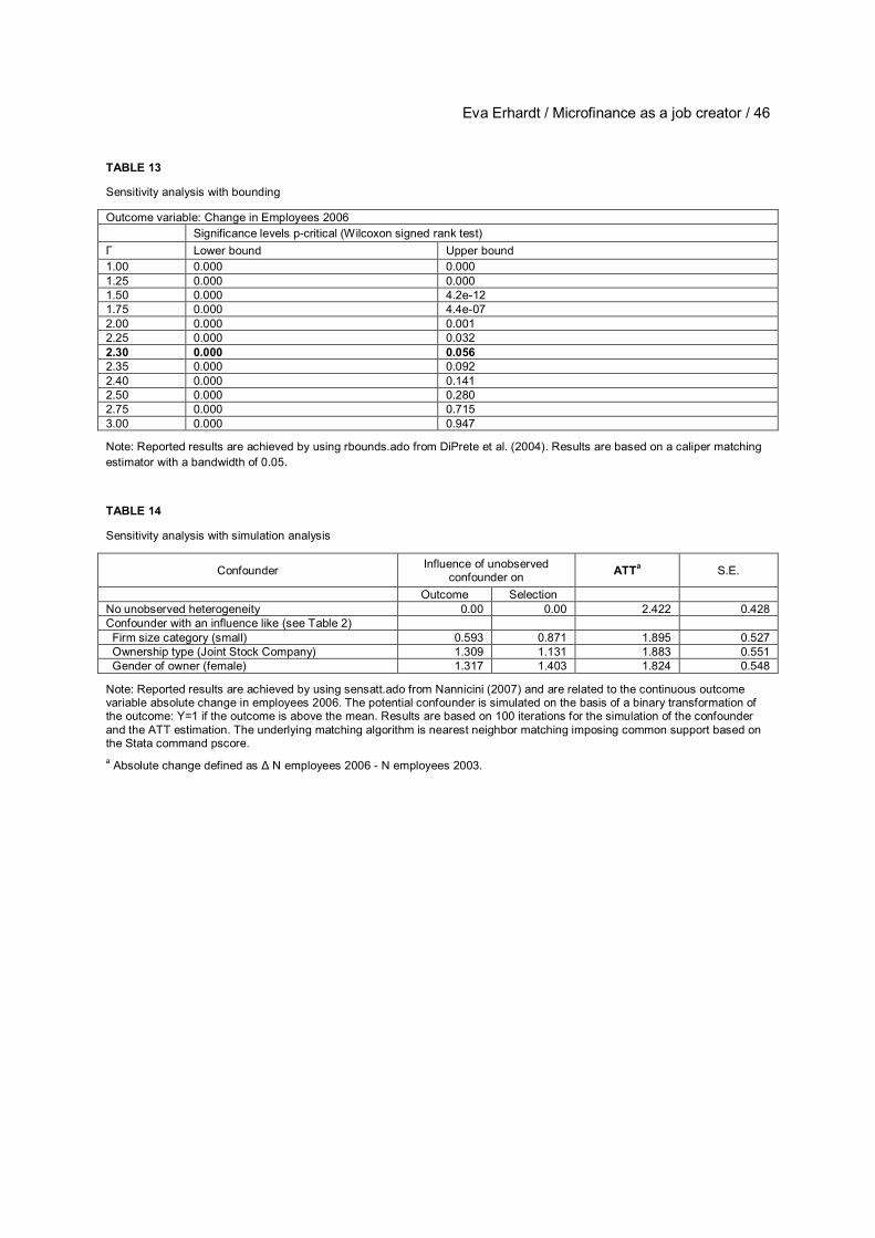
Eva Erhardt / Microfinance as a job creator / 46
TABLE 13
Sensitivity analysis with bounding
Outcome variable: Change in Employees 2006 Significance levels p-critical (Wilcoxon signed rank test) Γ Lower bound Upper bound 1.00 0.000 0.000 1.25 0.000 0.000 1.50 0.000 4.2e-12 1.75 0.000 4.4e-07 2.00 0.000 0.001 2.25 0.000 0.032 2.30 0.000 0.056 2.35 0.000 0.092 2.40 0.000 0.141 2.50 0.000 0.280 2.75 0.000 0.715 3.00 0.000 0.947
Note: Reported results are achieved by using rbounds.ado from DiPrete et al. (2004). Results are based on a caliper matching estimator with a bandwidth of 0.05.
TABLE 14
Sensitivity analysis with simulation analysis
Confounder Influence of unobserved confounder on ATTa S.E.
Outcome Selection No unobserved heterogeneity 0.00 0.00 2.422 0.428 Confounder with an influence like (see Table 2) Firm size category (small) 0.593 0.871 1.895 0.527 Ownership type (Joint Stock Company) 1.309 1.131 1.883 0.551 Gender of owner (female) 1.317 1.403 1.824 0.548
Note: Reported results are achieved by using sensatt.ado from Nannicini (2007) and are related to the continuous outcome variable absolute change in employees 2006. The potential confounder is simulated on the basis of a binary transformation of the outcome: Y=1 if the outcome is above the mean. Results are based on 100 iterations for the simulation of the confounder and the ATT estimation. The underlying matching algorithm is nearest neighbor matching imposing common support based on the Stata command pscore. a Absolute change defined as Δ N employees 2006 - N employees 2003.