m2 medical epidemiology how to fairly compare disease frequencies between groups
Post on 22-Dec-2015
216 views
TRANSCRIPT
M2 Medical Epidemiology
How to Fairly Compare Disease Frequencies Between Groups
How to Fairly Compare Disease Frequencies Between Groups
Simple epidemiologic indices: review/summary Interpreting epidemiologic comparisons:
overview– chance– bias– confounding
Adjustment of epidemiologic indices for confounding– direct– indirect
Simple epidemiologic indices: review/summary
Questions: What fraction of a group has the condition
now? What fraction of the community carries the
condition at any one time? What is the endemic level of the condition,
relative to the size of a community? What fraction of UI students has hay fever
now?
Simple epidemiologic indices: review/summary
Answer: Point prevalence, or prevalence for short. A dimensionless proportion. Sometimes erroneously called “prevalence
rate”
Simple epidemiologic indices: review/summary
Questions:
What is the cumulative risk (probability) of developing a condition at least once during a fixed time period?
What fraction of a group can we predict will have developed a condition over a given time period, or during an epidemic?
Why must I take this medicine, doctor? What are my chances of a heart attack in the next ten years, if I don't?
Simple epidemiologic indices: review/summary
Answers: Cumulative incidence A dimensionless proportion Called the attack rate when describing
infectious disease outbreaks, – e.g., The attack rate in the county during the West
Branch hepatitis outbreak was estimated as 6.5%=65 cases/1000 population.
One women in 11 (9%) is expected to develop breast cancer during her lifetime.
Simple epidemiologic indices: review/summary Questions:
How strong is the process causing new cases? How many new cases occur per person per unit
time, or other unit of experience (e.g., per passenger-trip, per passenger-mile traveled)?
How many new cases of esophageal cancer occur in Illinois/1000 population per year?
How many ruptured spleens occur from automotive accidents in Illinois, per million person-miles traveled?
How many new HIV infections occur per 1000 acts of vaginal intercourse? Of anal intercourse?
Simple epidemiologic indices: review/summary
Answer: Incidence density (rate, dimension = new
cases per unit of experience, such as person-year, passenger-mile, sexual acts) – e.g. 5 new cases per 1000 persons per year =
– 5 new cases per 1000 person-years =
– .005 new cases per person per year
Units = e.g.
– New cases / [persons x years]
– New cases / million passenger-miles
– New cases / 100 sexual acts
Simple epidemiologic indices: review/summary
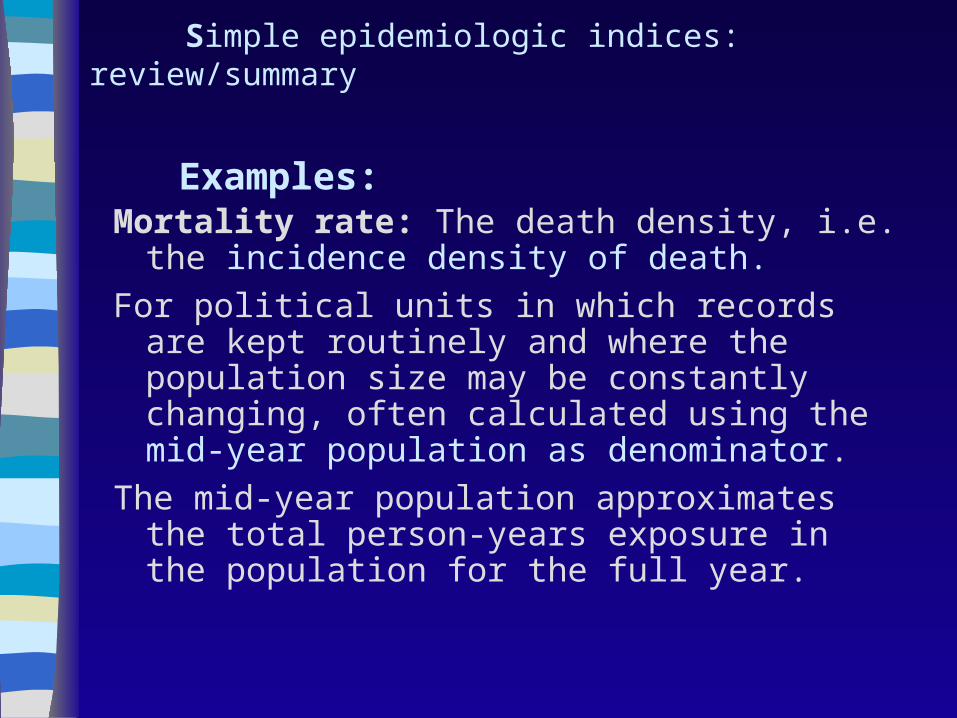
Examples: Mortality rate: The death density, i.e. the
incidence density of death.
For political units in which records are kept routinely and where the population size may be constantly changing, often calculated using the mid-year population as denominator.
The mid-year population approximates the total person-years exposure in the population for the full year.
10
Simple epidemiologic indices: review/summary
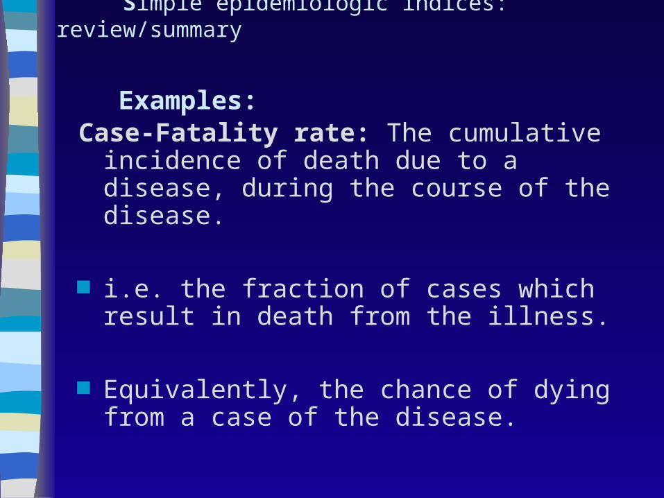
Examples: Case-Fatality rate: The cumulative incidence
of death due to a disease, during the course of the disease.
i.e. the fraction of cases which result in death from the illness.
Equivalently, the chance of dying from a case of the disease.
Case Fatality Rate
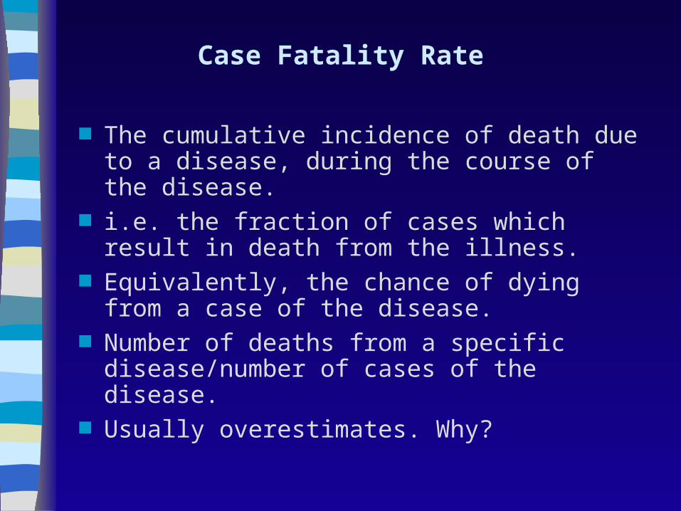
The cumulative incidence of death due to a disease, during the course of the disease.
i.e. the fraction of cases which result in death from the illness.
Equivalently, the chance of dying from a case of the disease.
Number of deaths from a specific disease/number of cases of the disease.
Usually overestimates. Why?
Simple epidemiologic indices: review/summary
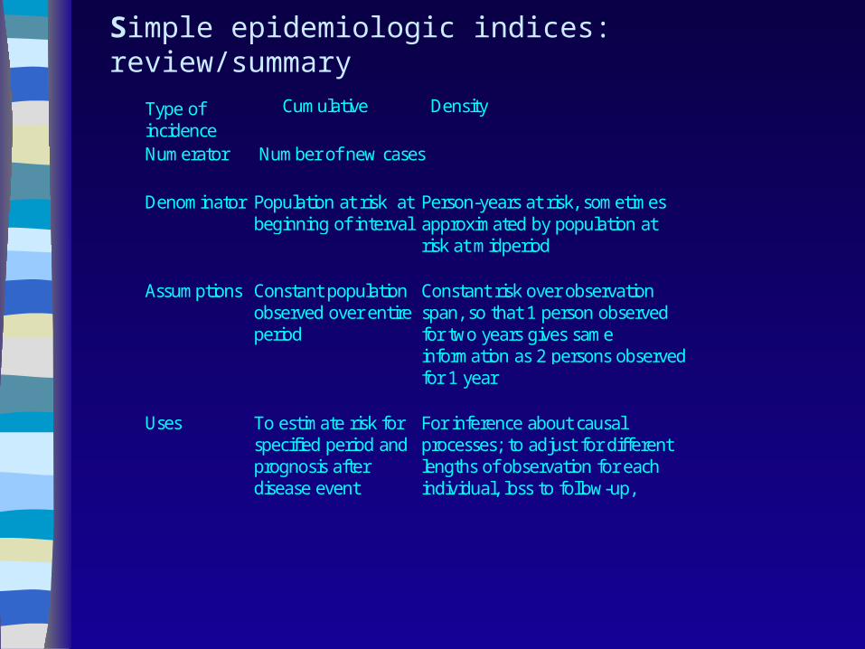
Type ofincidence
Cumulative Density
Numerator Number of new cases
Denominator Population at risk atbeginning of interval
Person-years at risk, sometimesapproximated by population atrisk at midperiod
Assumptions Constant populationobserved over entireperiod
Constant risk over observationspan, so that 1 person observedfor two years gives sameinformation as 2 persons observedfor 1 year
Uses To estimate risk forspecified period andprognosis afterdisease event
For inference about causalprocesses; to adjust for differentlengths of observation for eachindividual, loss to follow-up,
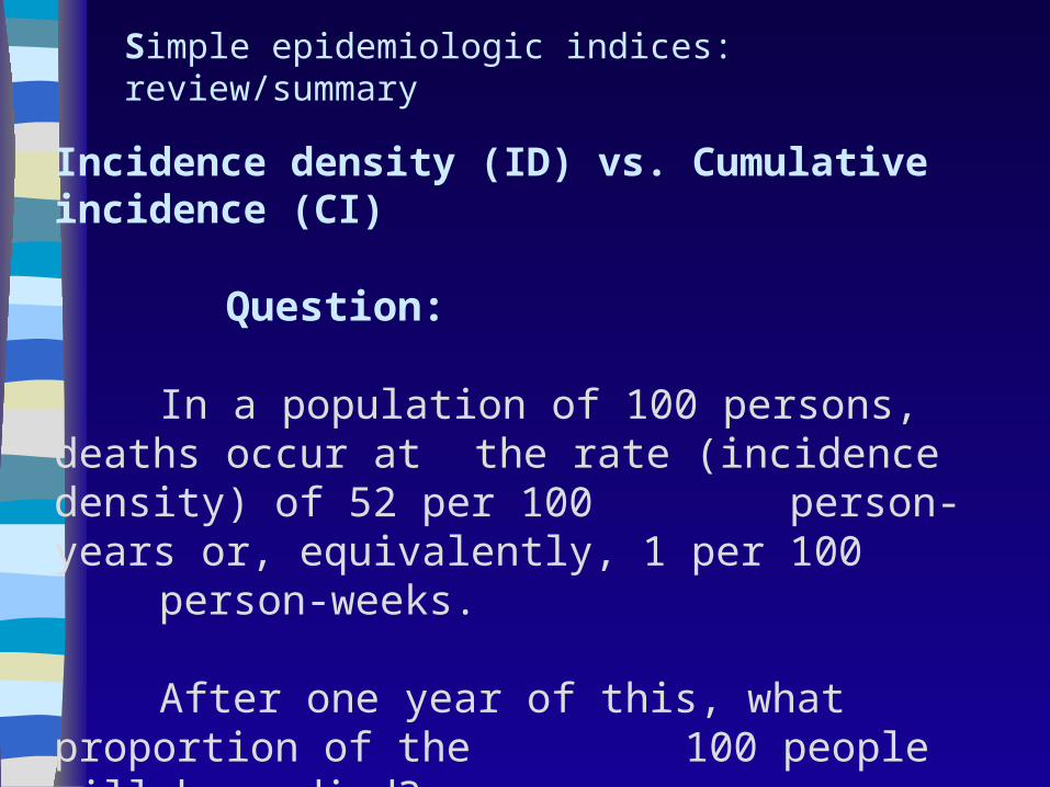
Simple epidemiologic indices: review/summary
Incidence density (ID) vs. Cumulative incidence (CI)
Question:
In a population of 100 persons, deaths occur at the rate (incidence density) of 52 per 100 person-years or, equivalently, 1 per 100 person-weeks.
After one year of this, what proportion of the 100 people will have died?
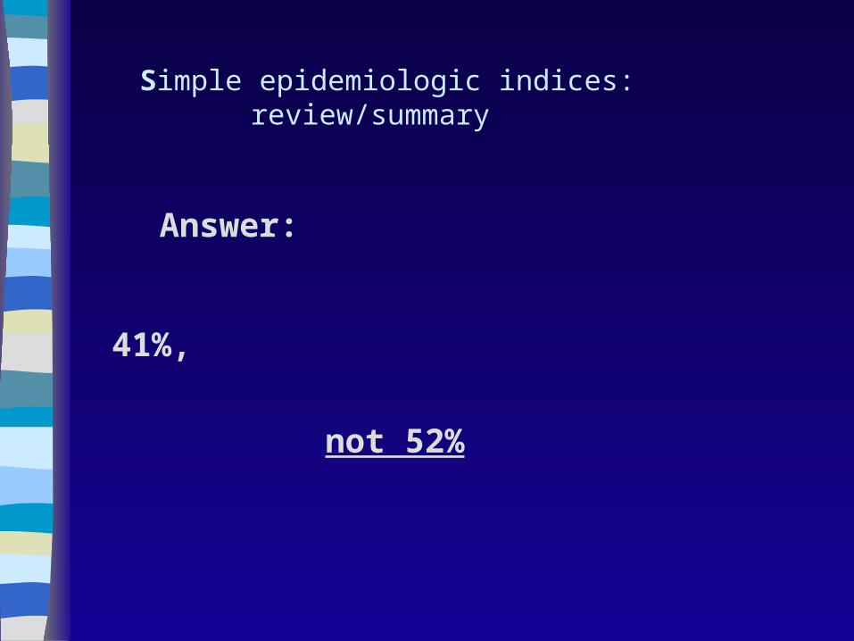
Simple epidemiologic indices: review/summary
Answer:
41%,
not 52%
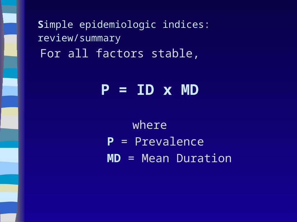
Simple epidemiologic indices: review/summary
For all factors stable,
P = ID x MD
where
P = Prevalence
MD = Mean Duration
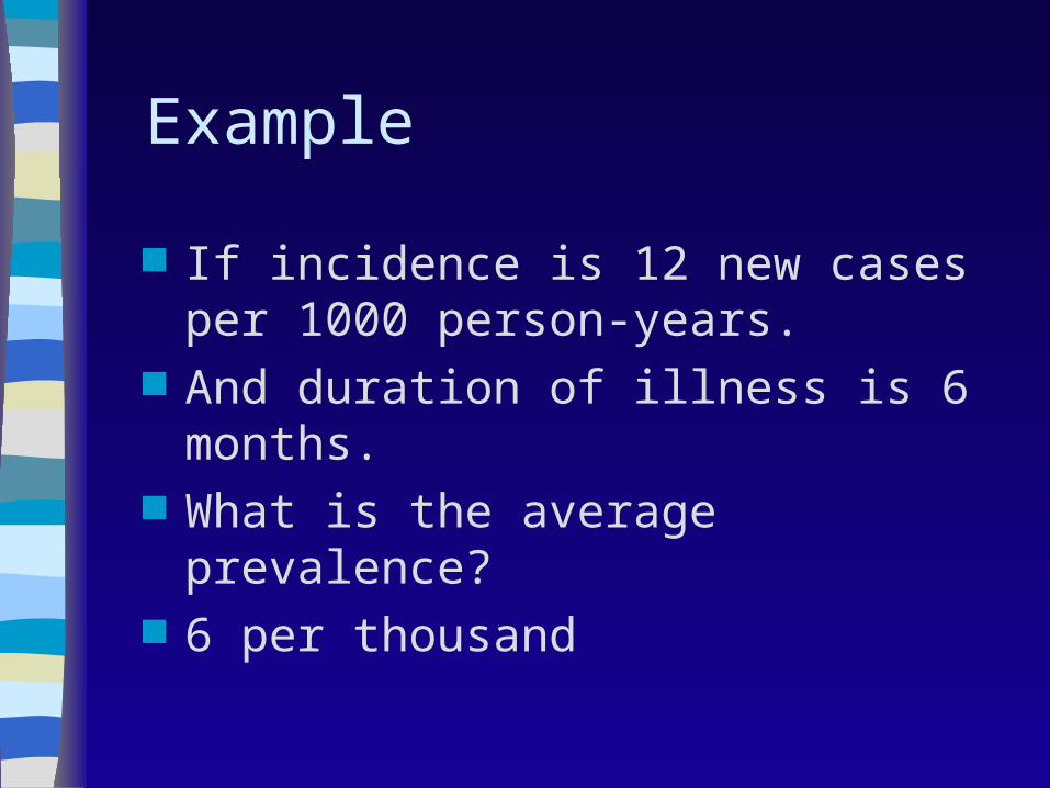
Example
If incidence is 12 new cases per 1000 person-years.
And duration of illness is 6 months. What is the average prevalence? 6 per thousand
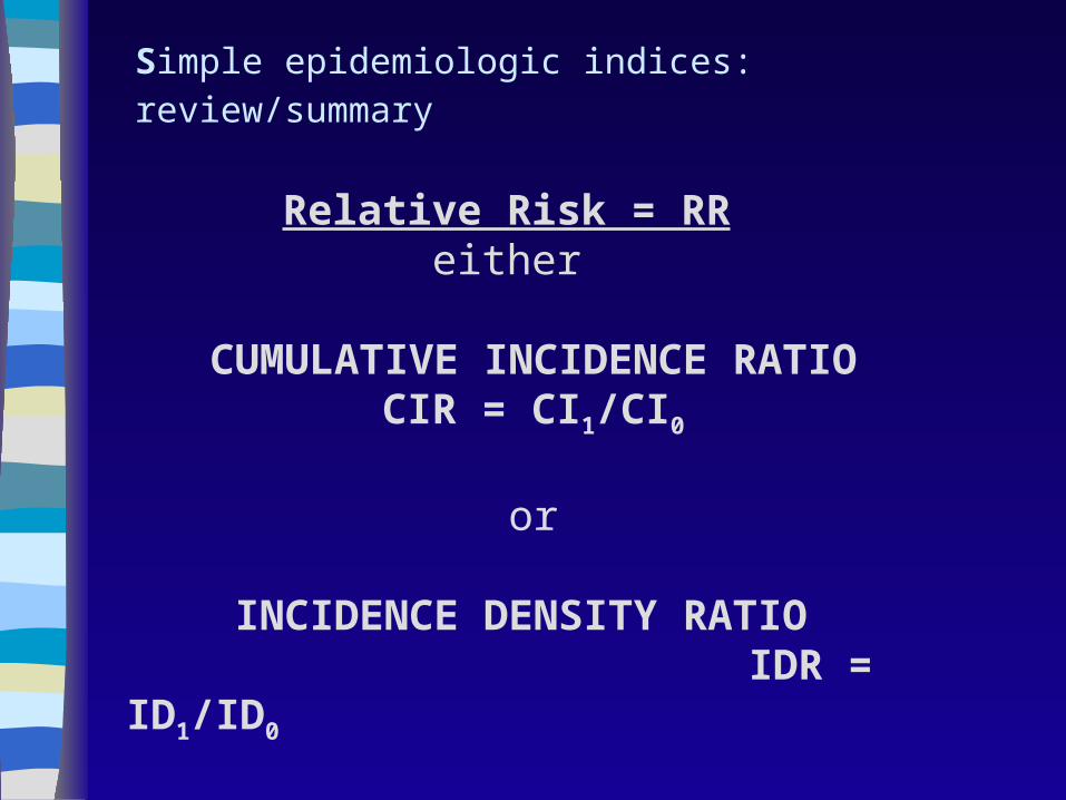
Simple epidemiologic indices: review/summary
Relative Risk = RReither
CUMULATIVE INCIDENCE RATIOCIR = CI1/CI0
or
INCIDENCE DENSITY RATIO IDR = ID1/ID0
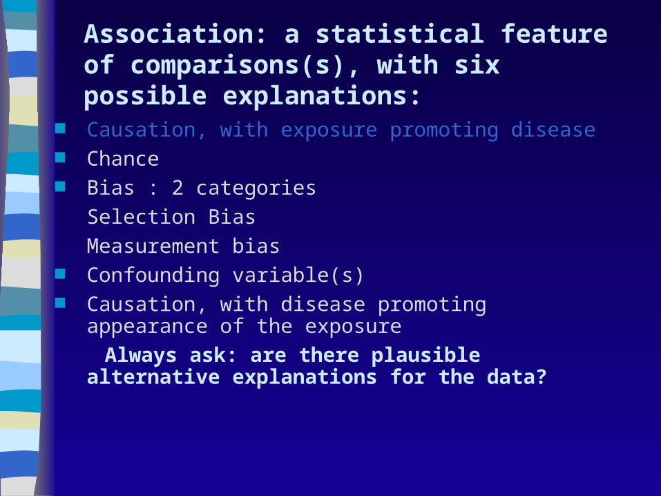
Association: a statistical feature of comparisons(s), with six possible explanations:
Causation, with exposure promoting disease Chance Bias : 2 categories
Selection Bias
Measurement bias Confounding variable(s) Causation, with disease promoting appearance of
the exposure
Always ask: are there plausible alternative explanations for the data?
Chance
due to random variation from sampling or measurement
addressed using– statistical tests of hypotheses (p-values)– confidence intervals– power analyses
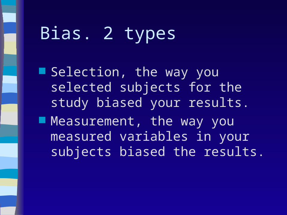
Bias. 2 types
Selection, the way you selected subjects for the study biased your results.
Measurement, the way you measured variables in your subjects biased the results.
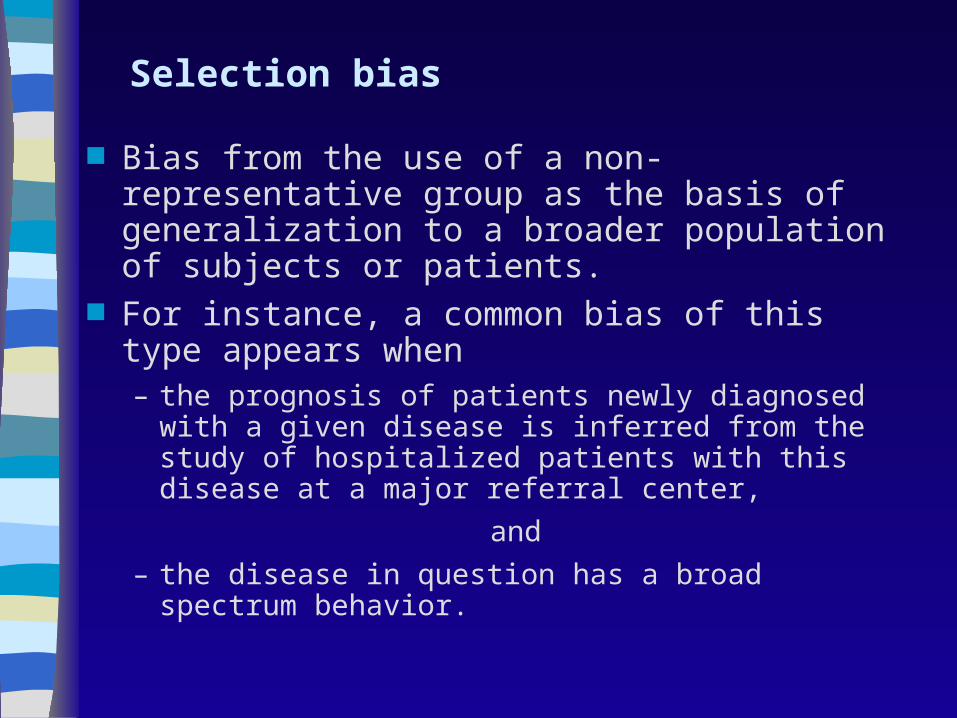
Selection bias
Bias from the use of a non-representative group as the basis of generalization to a broader population of subjects or patients.
For instance, a common bias of this type appears when – the prognosis of patients newly diagnosed with a
given disease is inferred from the study of hospitalized patients with this disease at a major referral center,
and
– the disease in question has a broad spectrum behavior.
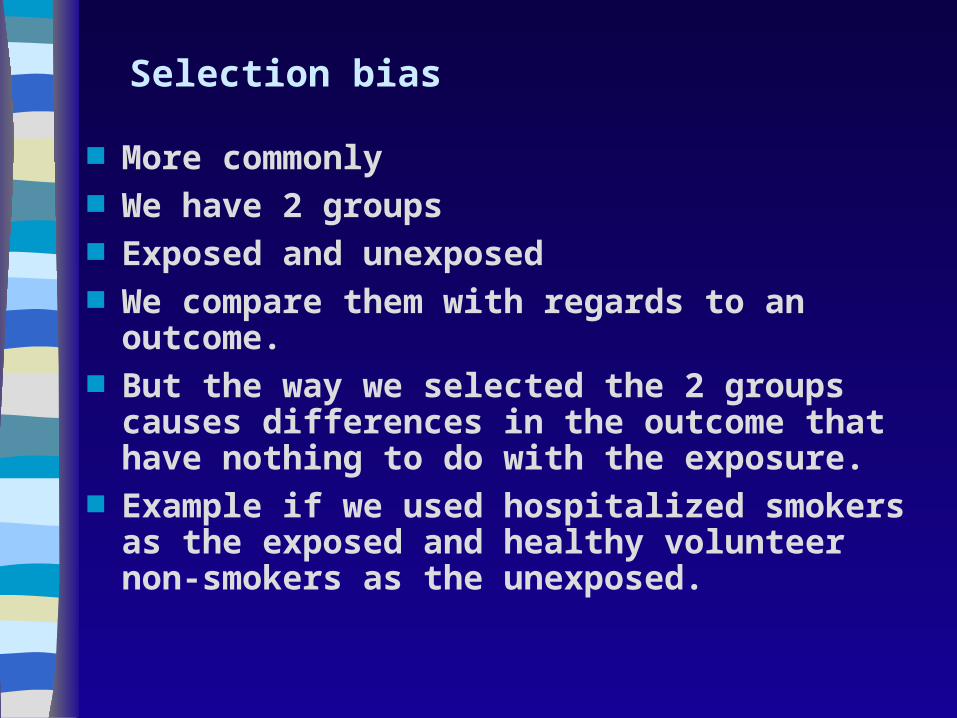
Selection bias
More commonly We have 2 groups Exposed and unexposed We compare them with regards to an
outcome. But the way we selected the 2 groups causes
differences in the outcome that have nothing to do with the exposure.
Example if we used hospitalized smokers as the exposed and healthy volunteer non-smokers as the unexposed.
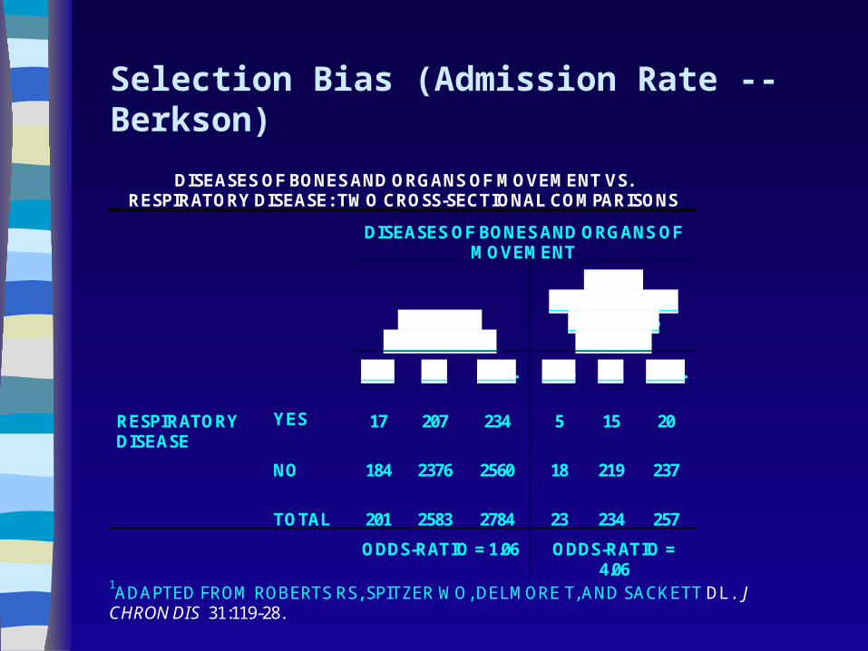
Selection Bias (Admission Rate -- Berkson)
DISEASES OF BONES AND ORGANS OF MOVEMENT VS.RESPIRATORY DISEASE: TWO CROSS-SECTIONAL COMPARISONS
DISEASES OF BONES AND ORGANS OFMOVEMENT
GENERAL POPULATION
THOSE HOSPITALIZED
IN PRIOR 6 MONTHS
YES NO TOT. YES NO TOT.
YES 17 207 234 5 15 20RESPIRATORYDISEASE
NO 184 2376 2560 18 219 237
TOTAL 201 2583 2784 23 234 257
ODDS-RATIO = 1.06 ODDS-RATIO =4.06
1ADAPTED FROM ROBERTS RS, SPITZER WO, DELMORE T, AND SACKETT DL. JCHRON DIS 31:119-28.
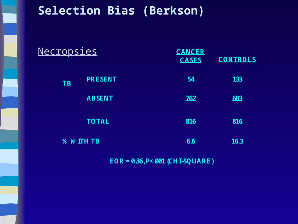
CANCER CASES
CONTROLS
PRESENT
54
133
TB ABSENT
762
683
TOTAL
816
816
% WITH TB
6.6
16.3
EOR = 0.36, P<.001 (CHI-SQUARE)
Selection Bias (Berkson) Necropsies
More Selection Biases Whenever we compare a group of
patients who use a drug to those who don’t in a non experimental observational study (cohort, not randomized).
The 2 groups differ in many respects. One of the most important respects is
that the patients on the drug have a reason to be on it (indication). The others don’t. Called “Bias by indication”.
Bias by indication
For example calcium channel blockers have 2 indications hypertension and coronary disease.
If you compare hypertensive patients who are on Ca blockers to those who are on other agents (not randomized, totally at the discretion of their doctors), we would find:
Bias by indication
Patient on Ca blockers have higher prevalence of CAD
Also higher prevalence of risk factors for CAD
So if you do an observational study of hypertensive patients, comparing the outcome in those on Ca blockers to those on other agents, you may find
Bias by indication
That patients on Ca blockers have much worse outcomes.
This is bias by indication. You can adjust and correct for
preexisting heart disease and for risk factors, but may not be enough.
Bias by indication
If you compare hypertensive patients who are on minoxidil or hydralazine to those on other agents you find
That patients on those agents have higher BP Is it because they don’t work as well ? No, the opposite. They are reserved for those
with severe resistant hypertension. That is the indication for those agents.
Survivor Treatment Bias
Patients who received statin during admission for MI had much lower in-hospital mortality.
Statin? The ones who died are different. Some died very soon after admission
(no statin).
Competing Medical Issues Bias
Some were so sick that they were treated with multiple drugs, modalities, ICU etc.
No statin
Bias by contraindication
If you compare hypertensive patients who are on beta blockers to those on other agents you find that they have better outcomes.
That does not mean they are better for you. No, this comparison is biased by contraindication.
Beta blockers are contraindicated in severe COPD, CHF, PVD etc.
Measurement bias
Systematic or non-uniform failure of a measurement process to accurately represent the measurement target, e.g.
– different approaches to questioning, when determining past exposures in a case-control study.
– more complete medical history and physical examination of subjects who have been exposed to an agent suspected of causing a disease than of those who haven't been exposed to the agent.
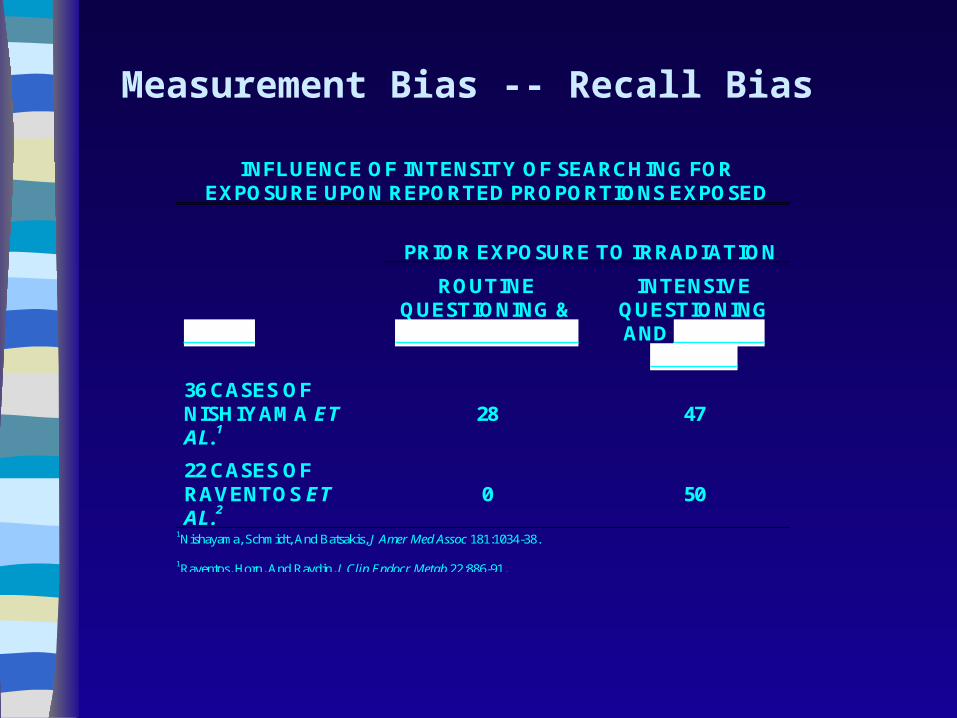
INFLUENCE OF INTENSITY OF SEARCHING FOREXPOSURE UPON REPORTED PROPORTIONS EXPOSED
PRIOR EXPOSURE TO IRRADIATION
STUDY
ROUTINEQUESTIONING &RECORD SEARCH
INTENSIVEQUESTIONINGAND RECORD
SEARCH
36 CASES OFNISHIYAMA ETAL.1
28 47
22 CASES OFRAVENTOS ETAL.2
0 50
1Nishayama, Schmidt, And Batsakis, J Amer Med Assoc 181:1034-38.
1Raventos, Horn, And Ravdin, J Clin Endocr Metab 22:886-91.
Measurement Bias -- Recall Bias
Measurement Bias
Family information bias
The flow of family information about exposures and illnesses
is stimulated by and directed to a new case in its midst.
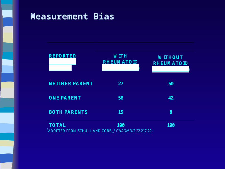
REPORTEDPARENTAL HISTORY
WITHRHEUMATOIDARTHRITIS (%)
WITHOUTRHEUMATOIDARTHRITIS (%)
NEITHER PARENT 27 50
ONE PARENT 58 42
BOTH PARENTS 15 8
TOTAL 100 1001ADOPTED FROM SCHULL AND COBB, J CHRON DIS 22:217-22.
Measurement Bias
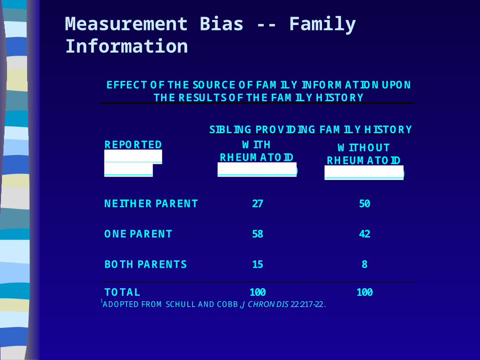
EFFECT OF THE SOURCE OF FAMILY INFORMATION UPONTHE RESULTS OF THE FAMILY HISTORY
SIBLING PROVIDING FAMILY HISTORY
REPORTEDPARENTAL HISTORY
WITHRHEUMATOIDARTHRITIS (%)
WITHOUTRHEUMATOIDARTHRITIS (%)
NEITHER PARENT 27 50
ONE PARENT 58 42
BOTH PARENTS 15 8
TOTAL 100 1001ADOPTED FROM SCHULL AND COBB, J CHRON DIS 22:217-22.
Measurement Bias -- Family Information
Avoid confounding
Confounding refers to distortion of the true biologic relation between an exposure and a disease outcome of interest, due to a research design and analysis that fail to properly account for additional variables associated with both. Such variables are referred to as confounders or, less formally, as lurking variables.
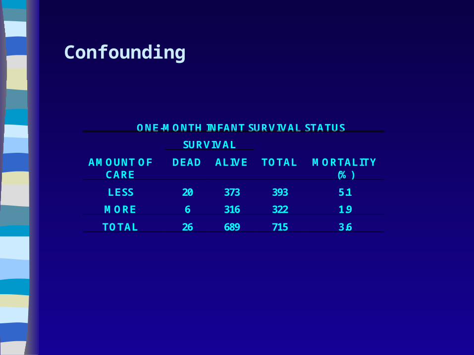
ONE-MONTH INFANT SURVIVAL STATUS
SURVIVAL
AMOUNT OFCARE
DEAD ALIVE TOTAL MORTALITY(%)
LESS 20 373 393 5.1
MORE 6 316 322 1.9
TOTAL 26 689 715 3.6
Confounding
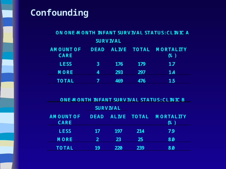
ON ONE-MONTH INFANT SURVIVAL STATUS: CLINIC A
SURVIVAL
AMOUNT OFCARE
DEAD ALIVE TOTAL MORTALITY(%)
LESS 3 176 179 1.7
MORE 4 293 297 1.4
TOTAL 7 469 476 1.5
ONE-MONTH INFANT SURVIVAL STATUS: CLINIC B
SURVIVAL
AMOUNT OFCARE
DEAD ALIVE TOTAL MORTALITY(%)
LESS 17 197 214 7.9
MORE 2 23 25 8.0
TOTAL 19 220 239 8.0
Confounding
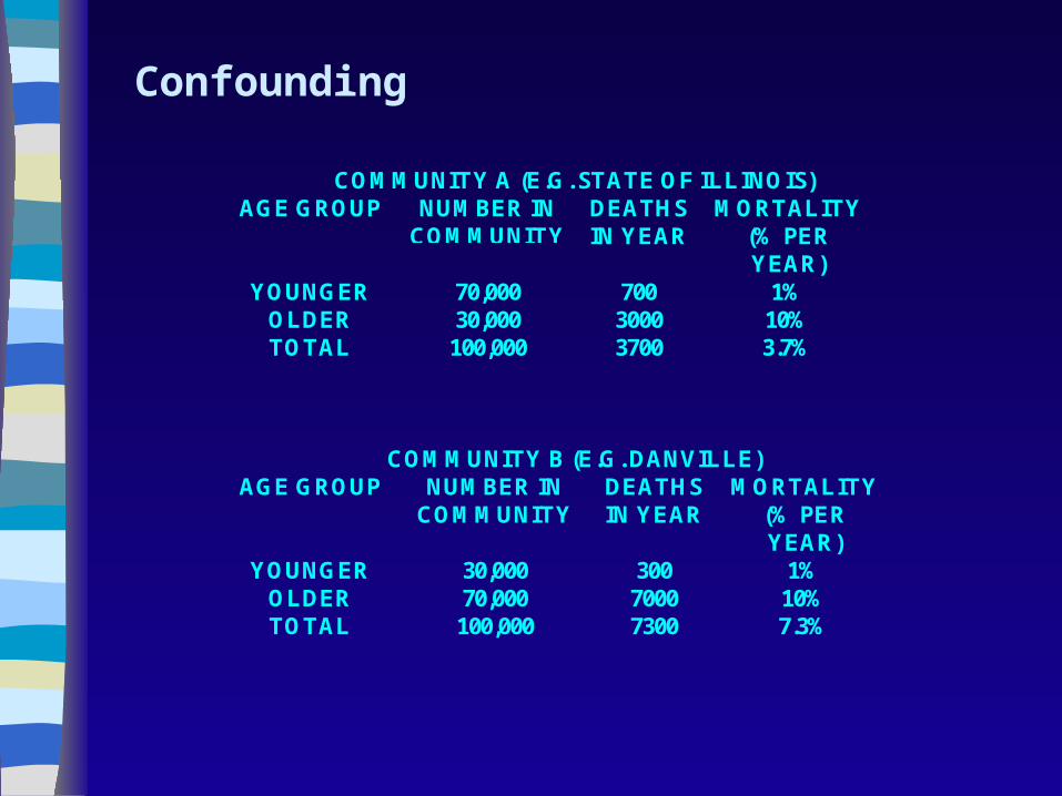
COMMUNITY A (E.G. STATE OF ILLINOIS)AGE GROUP NUMBER IN
COMMUNITYDEATHSIN YEAR
MORTALITY(% PERYEAR)
YOUNGER 70,000 700 1%OLDER 30,000 3000 10%TOTAL 100,000 3700 3.7%
COMMUNITY B (E.G. DANVILLE)AGE GROUP NUMBER IN
COMMUNITYDEATHSIN YEAR
MORTALITY(% PERYEAR)
YOUNGER 30,000 300 1%OLDER 70,000 7000 10%TOTAL 100,000 7300 7.3%
Confounding
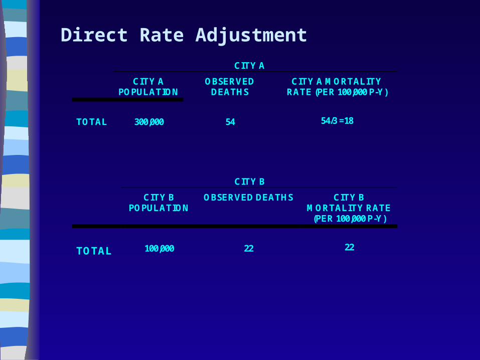
CITY A
CITY APOPULATION
OBSERVEDDEATHS
CITY A MORTALITYRATE (PER 100,000 P-Y)
TOTAL 300,000 54 54/3 =18
CITY B
CITY BPOPULATION
OBSERVED DEATHS CITY BMORTALITY RATE
(PER 100,000 P-Y)
TOTAL 100,000 22 22
Direct Rate Adjustment
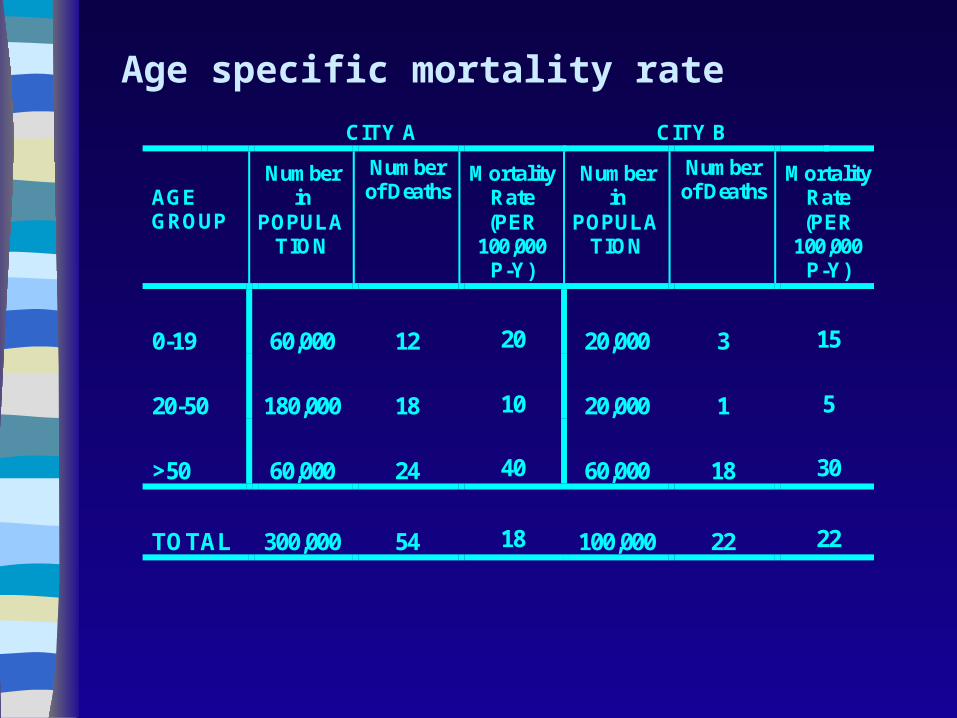
CITY A CITY B
AGEGROUP
Numberin
POPULATION
Numberof Deaths
MortalityRate(PER
100,000P-Y)
Numberin
POPULATION
Numberof Deaths
MortalityRate(PER
100,000P-Y)
0-19 60,000 12 20 20,000 3 15
20-50 180,000 18 10 20,000 1 5
>50 60,000 24 40 60,000 18 30
TOTAL 300,000 54 18 100,000 22 22
Age specific mortality rate
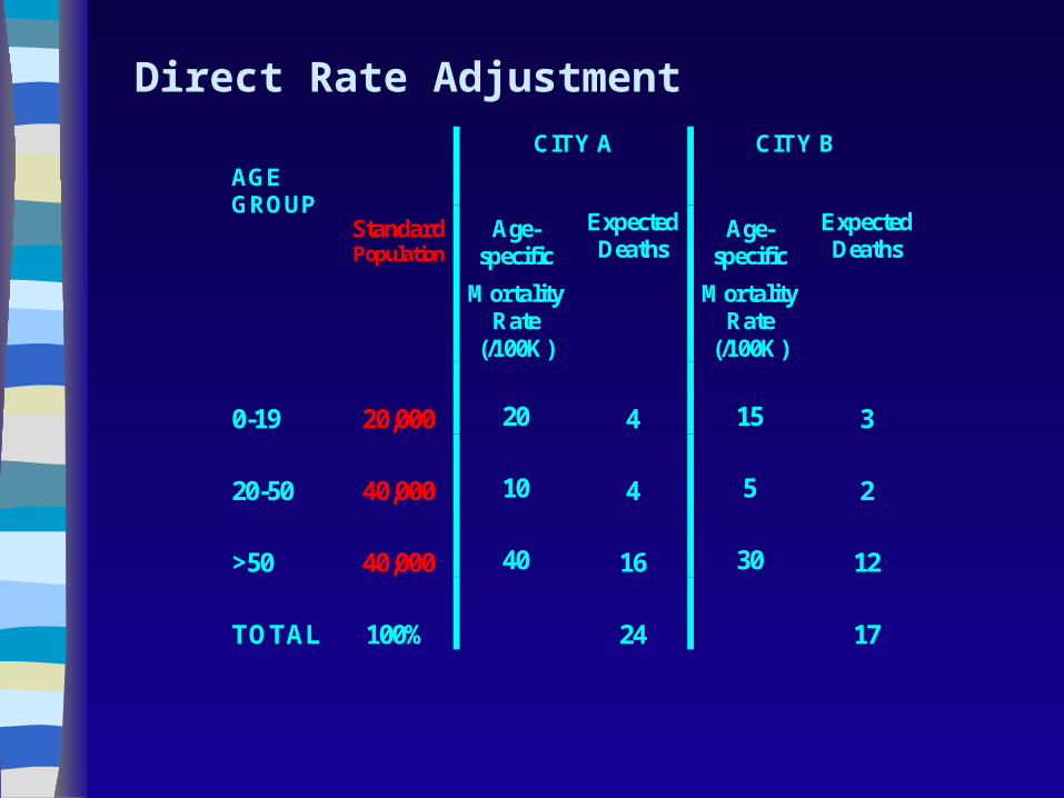
CITY A CITY B
AGE GROUP
Standard Population
Age-specific
Mortality Rate
(/100K)
Expected Deaths
Age-specific
Mortality Rate
(/100K)
Expected Deaths
0-19
20,000
20
4
15
3
20-50
40,000
10
4
5
2
>50
40,000
40
16
30
12
TOTAL
100%
24
17
Direct Rate Adjustment
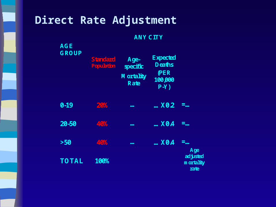
ANY CITY
AGE GROUP
Standard Population
Age-specific
Mortality Rate
Expected Deaths (PER
100,000 P-Y)
0-19
20%
…
…X0.2
=…
20-50
40%
…
…X0.4
=…
>50
40%
…
…X0.4
=…
TOTAL
100%
Age adjusted mortality
rate
Direct Rate Adjustment
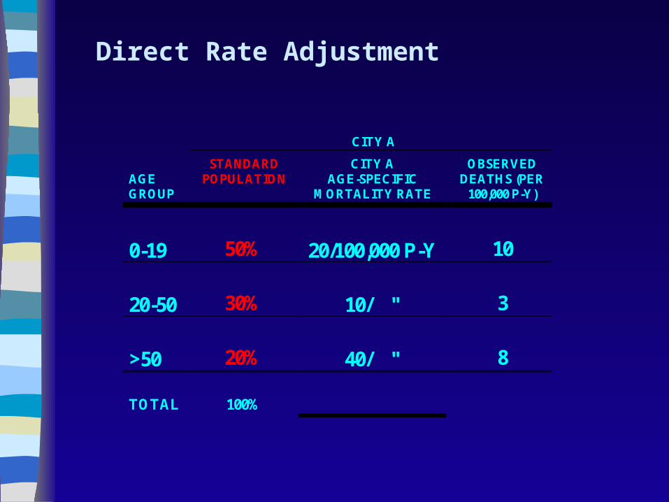
Direct Rate Adjustment
CITY A
AGE GROUP
STANDARD POPULATION
CITY A AGE-SPECIFIC
MORTALITY RATE
OBSERVED DEATHS (PER
100,000 P-Y)
0-19
50%
20/100,000 P-Y
10
20-50
30%
10/ "
3
>50
20%
40/ "
8
TOTAL
100%
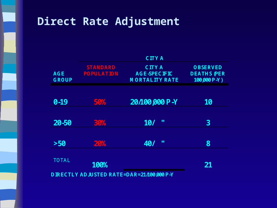
Direct Rate Adjustment
CITY A
AGE GROUP
STANDARD POPULATION
CITY A AGE-SPECIFIC
MORTALITY RATE
OBSERVED DEATHS (PER
100,000 P-Y)
0-19
50%
20/100,000 P-Y
10
20-50
30%
10/ "
3
>50
20%
40/ "
8
TOTAL
100%
21
DIRECTLY ADJUSTED RATE=DAR=21/100,000 P-Y
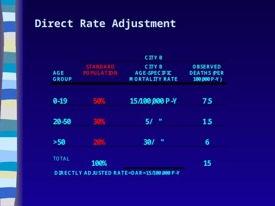
Direct Rate Adjustment
CITY B
AGE GROUP
STANDARD POPULATION
CITY B AGE-SPECIFIC
MORTALITY RATE
OBSERVED DEATHS (PER
100,000 P-Y)
0-19
50%
15/100,000 P-Y
7.5
20-50
30%
5/ "
1.5
>50
20%
30/ "
6
TOTAL
100%
15
DIRECTLY ADJUSTED RATE=DAR=15/100,000 P-Y
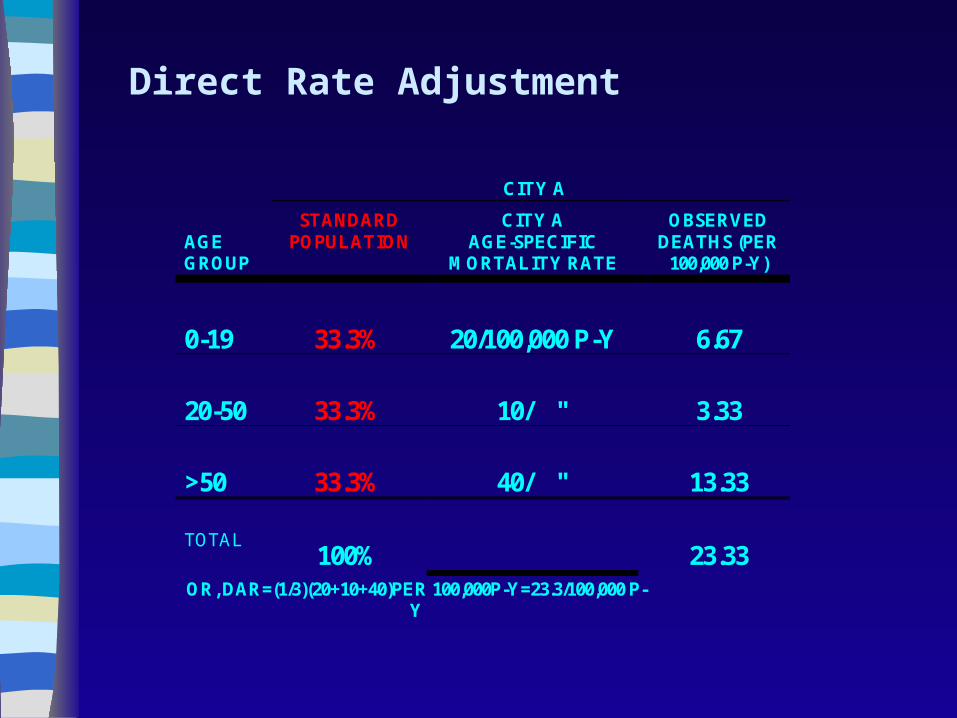
Direct Rate Adjustment
CITY A
AGE GROUP
STANDARD POPULATION
CITY A AGE-SPECIFIC
MORTALITY RATE
OBSERVED DEATHS (PER
100,000 P-Y)
0-19
33.3%
20/100,000 P-Y
6.67
20-50
33.3%
10/ "
3.33
>50
33.3%
40/ "
13.33
TOTAL
100%
23.33
OR, DAR=(1/3)(20+10+40)PER 100,000P-Y=23.3/100,000 P-Y
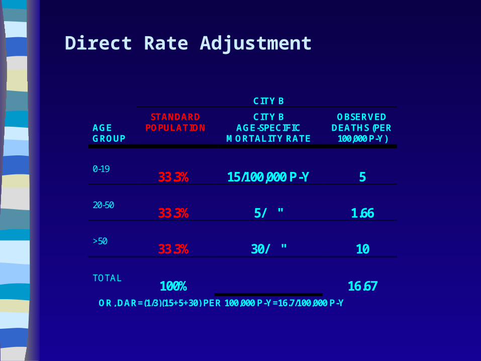
Direct Rate Adjustment
CITY B
AGE GROUP
STANDARD POPULATION
CITY B AGE-SPECIFIC
MORTALITY RATE
OBSERVED DEATHS (PER
100,000 P-Y)
0-19
33.3%
15/100,000 P-Y
5
20-50
33.3%
5/ "
1.66
>50
33.3%
30/ "
10
TOTAL
100%
16.67
OR, DAR=(1/3)(15+5+30) PER 100,000 P-Y=16.7/100,000 P-Y
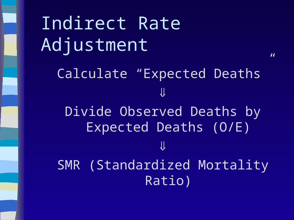
Indirect Rate Adjustment
Calculate “Expected Deaths”
Divide Observed Deaths by Expected
Deaths (O/E)
SMR (Standardized Mortality Ratio)
Indirect Rate Adjustment
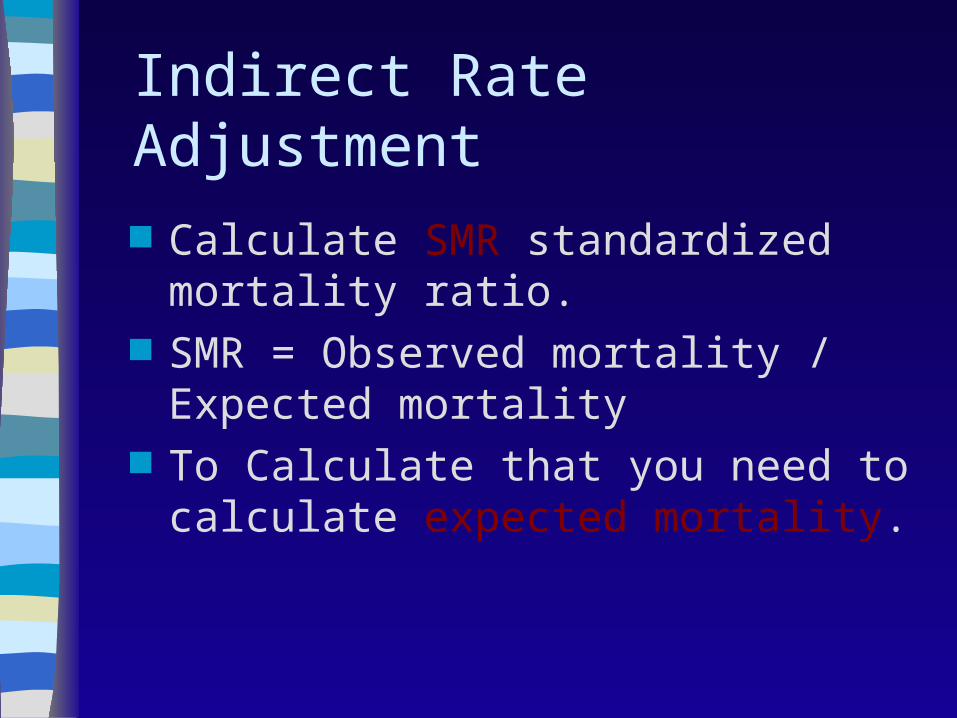
Calculate SMR standardized mortality ratio.
SMR = Observed mortality / Expected mortality
To Calculate that you need to calculate expected mortality.
Indirect Rate Adjustment
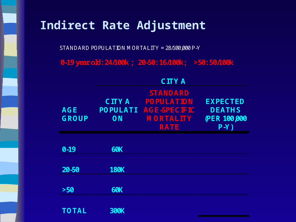
STANDARD POPULATION MORTALITY = 28/100,000 P-Y
0-19 year old: 24/100k ; 20-50: 16/100k; >50: 50/100k
CITY A
AGE GROUP
CITY A
POPULATION
STANDARD POPULATION AGE-SPECIFIC MORTALITY
RATE
EXPECTED
DEATHS (PER 100,000
P-Y)
0-19
60K
20-50
180K
>50
60K
TOTAL
300K
Indirect Rate Adjustment
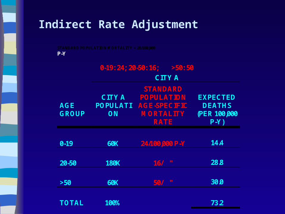
STANDARD POPULATION MORTALITY = 28/100,000 P-Y
0-19: 24; 20-50: 16; >50: 50
CITY A
AGE GROUP
CITY A
POPULATION
STANDARD POPULATION AGE-SPECIFIC MORTALITY
RATE
EXPECTED
DEATHS (PER 100,000
P-Y)
0-19
60K
24/100,000 P-Y
14.4
20-50
180K
16/ "
28.8
>50
60K
50/ "
30.0
TOTAL
100%
73.2

Indirect Rate Adjustment
Calculate “Expected Deaths”
Divide Observed Deaths by Expected
Deaths (O/E)
SMR (Standardized Mortality Ratio)
Indirect Rate Adjustment
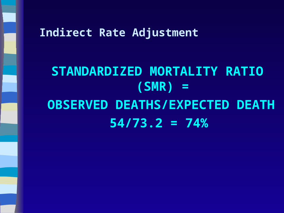
STANDARDIZED MORTALITY RATIO (SMR) =
OBSERVED DEATHS/EXPECTED DEATH
54/73.2 = 74%
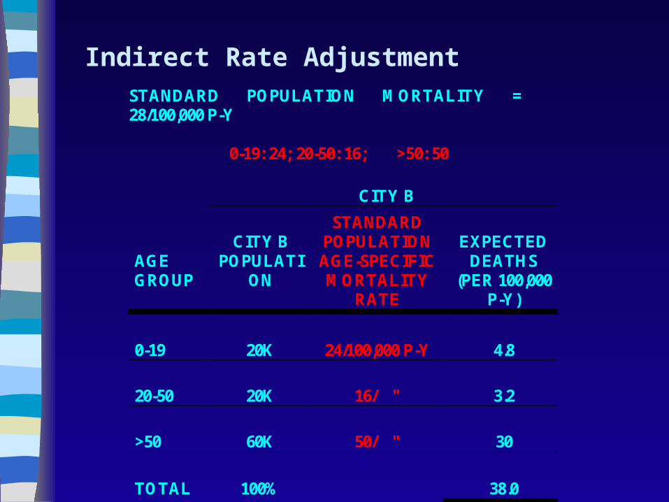
Indirect Rate AdjustmentSTANDARD POPULATION MORTALITY = 28/100,000 P-Y 0-19: 24; 20-50: 16; >50: 50
CITY B
AGE GROUP
CITY B
POPULATION
STANDARD POPULATION AGE-SPECIFIC MORTALITY
RATE
EXPECTED
DEATHS (PER 100,000
P-Y)
0-19
20K
24/100,000 P-Y
4.8
20-50
20K
16/ "
3.2
>50
60K
50/ "
30
TOTAL
100%
38.0
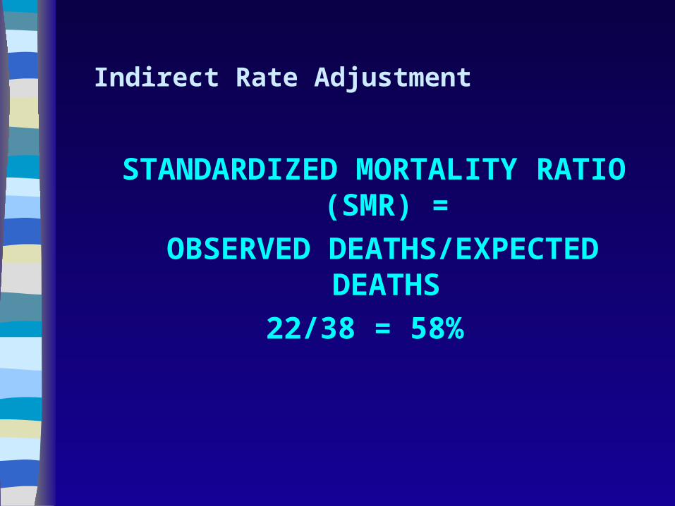
Indirect Rate Adjustment
STANDARDIZED MORTALITY RATIO (SMR) =
OBSERVED DEATHS/EXPECTED DEATHS
22/38 = 58%
Proportional Mortality
The 4 leading causes of death in Chamapign County are….
CAD is the leading cause being responsible for 32% of all deaths in the County in 2002.

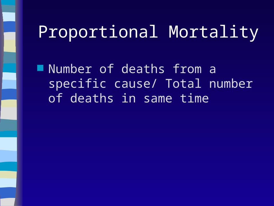
Proportional Mortality
Number of deaths from a specific cause/ Total number of deaths in same time
Proportional Mortality RatioPMR
Proportional Mortality Ratio
Proportion of deaths from specified cause /Proportion of deaths from specified cause in comparison population
Proportional Mortality RatioPMR
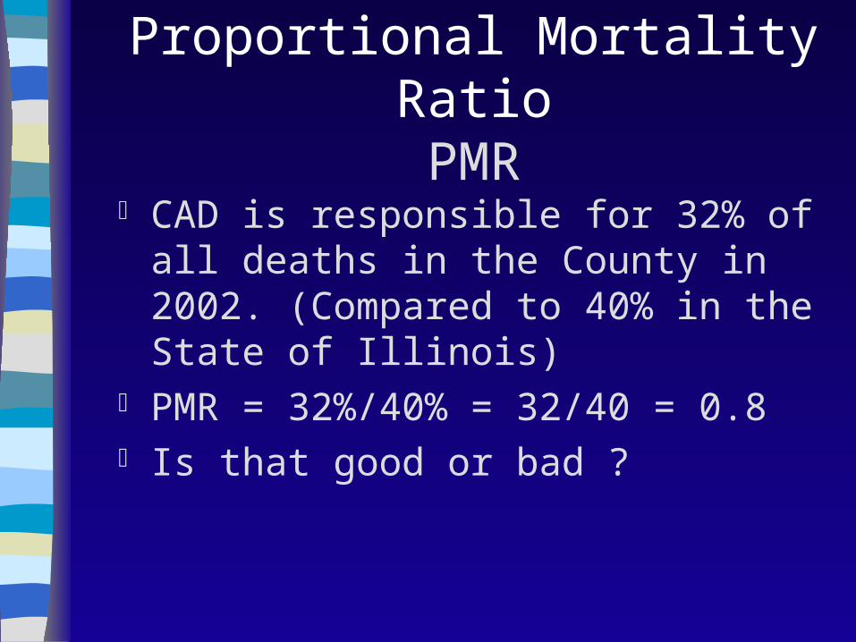
CAD is responsible for 32% of all deaths in the County in 2002. (Compared to 40% in the State of Illinois)
PMR = 32%/40% = 32/40 = 0.8 Is that good or bad ?
PMRRelative frequency of other causes of death can
affect the PMR for the cause of interest
An epidemic of a fatal disease in your population will decrease PMR for all other causes
Low mortality from a very common cause (CAD for example) in your population will increase PMR for all other causes
PMR
Fast, easy, cheap Can be calculated when all you have is
death certificates Don’t need information on demography
of population. “Leading Causes of Death”
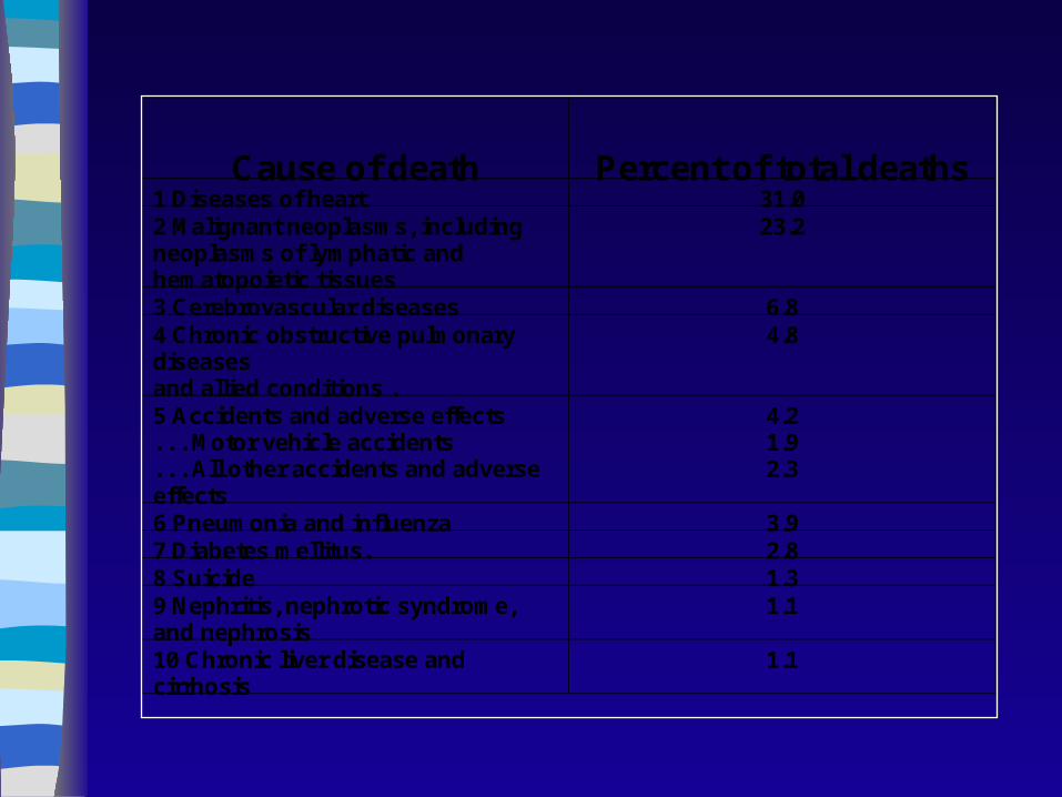
Cause of death Percent of total deaths1 Diseases of heart 31.02 Malignant neoplasms, includingneoplasms of lymphatic andhematopoietic tissues
23.2
3 Cerebrovascular diseases 6.84 Chronic obstructive pulmonarydiseasesand allied conditions .
4.8
5 Accidents and adverse effects. . . Motor vehicle accidents. . . All other accidents and adverseeffects
4.21.92.3
6 Pneumonia and influenza 3.97 Diabetes mellitus. 2.88 Suicide 1.39 Nephritis, nephrotic syndrome,and nephrosis
1.1
10 Chronic liver disease andcirrhosis
1.1
How does one decide whether to present a set of data using crude, adjusted, or category-specific indices?
If possible, use crude indices only to produce a quick picture of the magnitude of a problem in a population, for the purpose of establishing a prima facie need for public health and/or medical services, and as a first-cut at estimating the resources needed.
How does one decide whether to present a set of data using crude, adjusted, or category-specific indices?
Use category-specific indices when you wish to focus attention on the problem in one or a few population subgroups, when space is available to give a detailed presentation in order to communicate the fullest understanding of the data, and especially if specific indices vary between two populations being compared in a different manner in different population subgroups (e.g. effects are modified by age, sex or race).
How does one decide whether to present a set of data using crude, adjusted, or category-specific indices?
Use adjusted rates when – you wish to avoid possible confounding, – but do not have the space to present the full
schedules of specific indices, or your audience does not have the patience for that,
Avoid adjusted rates when– there variable being adjusted out is an
“effect modifier,” that is, the relationship between groups being compared changes from stratum to stratum -- more later on this.
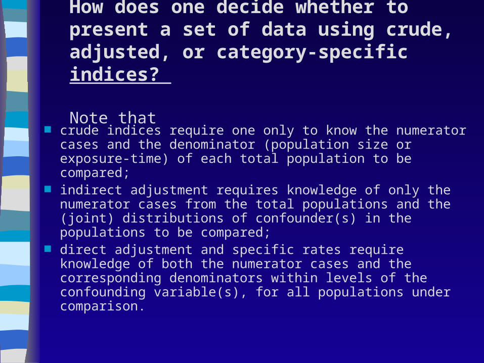
How does one decide whether to present a set of data using crude, adjusted, or category-specific indices?
Note that crude indices require one only to know the numerator
cases and the denominator (population size or exposure-time) of each total population to be compared;
indirect adjustment requires knowledge of only the numerator cases from the total populations and the (joint) distributions of confounder(s) in the populations to be compared;
direct adjustment and specific rates require knowledge of both the numerator cases and the corresponding denominators within levels of the confounding variable(s), for all populations under comparison.
Note that
A directly adjusted rate of a single community means nothing by itself. It is only used to compare different communities and only if all of them are adjusted to the same standard population.
SMR of a single community IS useful. It does by itself compare 2 populations.