m3-4-5 a16 notes for geometric mechanics: rigid body, mid

M3-4-5 A16 Notes for Geometric Mechanics:Rigid Body, mid Oct – mid Nov 2011

Professor Darryl D Holm 25 October 2011Imperial College London [email protected]

http://www.ma.ic.ac.uk/~dholm/

Text for the course:

Geometric Mechanics I: Dynamics and Symmetry,by Darryl D HolmWorld Scientific: Imperial College Press, Singapore, Second edition (2011).ISBN 978-1-84816-195-5

Where are we going in this course?

1. Euler–Poincare equation

2. Rigid body

3. Spherical pendulum

4. Elastic spherical pendulum

5. Differential forms

e

Where have we been so far?

• Mathematical setting for geometric mechanics, first on manifolds, then on (matrix) Liegroups

– Manifold M 'loc Rn e.g., n = 1 (scalars), n = m (m-vectors), n = m × m(matrices),

1

Notes for Geometric Mechanics: Rigid body DD Holm Oct–Nov 2011 2

– Motion equation on TM : q(t) = f(q) =⇒ transformation theory (pullbacks andall that)

– Hamilton’s principle for Lagrangian L : TM → R vector fields

∗ Euler–Lagrange equations on T ∗M

∗ Hamilton’s canonical equations on T ∗M

∗ Euler–Poincare eqns on T ∗eG ' g∗ for reduced Lagrangian ` : g → R, e.g.,rigid body.

Figure 1: The fabric of geometric mechanics is woven by a network of fundamental contri-butions by at least a dozen people to the dual fields of optics and motion.

1 Euler–Poincare Theorem

The definition of an invariant (or symmetric) function under a group action is as follows:

Definition 1.1. Let G act on TG by left translation. A function F : TG→ R is called leftinvariant if and only if

F (h(g, g)) = F (g, g) for all (g, g) ∈ TG ,

whereh(g, g) := (gh, TeLg(h)) .


If the Lagrangian is left invariant, then:

L(g, g) = L(g−1g, g−1g) = L(e, g−1g) = L(e, ξ) for all (g, g) ∈ TG,

where ξ := g−1g. Note that in this case the Lagrangian satisfies

L(g, g) = L(e, ξ),

so it is independent of g.This equation can be re-expressed as

d

dt

(δl

δξ

)= ad∗ξ

δl

δξ,

where l is defined to be the restriction of L to g:

l : g→ R , l(ξ) := L(e, ξ) for all g ∈ ξ .

The following theorem is now easily verified:

Theorem 1.1 (Euler–Poincare reduction). Let G be a Lie group, L : TG → R a left-invariant Lagrangian, and define the reduced Lagrangian,

l : g→ R, l(ξ) := L(e, ξ) ,

as the restriction of L to g. For a curve g(t) ∈ G, let

ξ(t) = g(t)−1g(t) := Tg(t)Lg(t)−1 g(t) ∈ g .

Then, the following four statements are equivalent:

(i) The variational principle

δ

∫ b

a

L(g(t), g(t))dt = 0

holds, for variations among paths with fixed endpoints.

(ii) g(t) satisfies the Euler–Lagrange equations for Lagrangian L defined on G.

(iii) The variational principle

δ

∫ b

a

l(ξ(t))dt = 0

holds on g, using variations of the form δξ = η+ [ξ, η], where η(t) is an arbitrary pathin g that vanishes at the endpoints, i.e. η(a) = 0 = η(b).

(iv) The (left invariant) Euler–Poincare equations hold:

d

dt

δl

δξ= ad∗ξ

δl

δξ,

where 〈ad∗ξµ, η〉 := 〈µ, adξη〉, for µ ∈ g∗ and ξ, η ∈ g.


Remark 1.1. A similar statement holds, with obvious changes for right-invari-ant Lagrangian systems on TG. In this case the Euler-Poincare equations are given by:

d

dt

δl

δξ= − ad∗ξ

δl

δξ, (1.1)

with the opposite sign.

Exercise. [Components of ad∗ξµ]

If µ = µiei, ξ = ξjej and η = ηkek, with [ej, ek] = cljkel and 〈ei, ej〉 = δji , show

that(ad∗ξµ)k = ξjµic

ijk .

F

Reconstruction

The reconstruction of the solution g(t) of the Euler–Lagrange equations, with initial condi-tions g(0) = g0 and g(0) = v0, is as follows: first, solve the initial value problem for the rightinvariant Euler–Poincare equations:

d

dt

δl

δξ= ad∗ξ

δl

δξwith ξ(0) = ξ0 := g−1

0 v0 .

Second, using the solution ξ(t) of the above, find the curve g(t) ∈ G by solving the recon-struction equation

g(t) = g(t)ξ(t) with g(0) = g0 ,

which is a differential equation with time-dependent coefficients.

Exercise. Prove the Euler–Poincare reduction Theorem 1.1. F

Exercise. Write out the proof of the Euler–Poincare reduction theorem for right-invariant Lagrangians and describe the corresponding reconstruction procedure.

F

Exercise. [Motion on SO(4)]Write out the Euler–Poincare equations in matrix form for a free rigid body fixedat its centre of mass in a 4-dimensional space. Use the analogue of the ‘hat’ mapfor so(4) and write the R6 vector representation of the equations. F

Exercise. Consider the following action of a Lie group G on a product spaceG× Y, where Y is some manifold:

(g , (h, y))→ (gh, y).

Let L : T (G × Y ) → R be invariant with respect to this action. Define l :g× TY → R as the restriction of L, i.e.

l(ξ, y, y) := L(e, ξ, y, y).


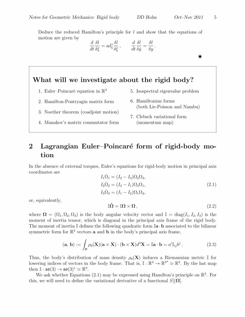
Deduce the reduced Hamilton’s principle for l and show that the equations ofmotion are given by

d

dt

δl

δξ= ad∗ξ

δl

δξ,

d

dt

δl

δy=δl

δy.

F

What will we investigate about the rigid body?

1. Euler–Poincare equation in R3

2. Hamilton-Pontryagin matrix form

3. Noether theorem (coadjoint motion)

4. Manakov’s matrix commutator form

5. Isospectral eigenvalue problem

6. Hamiltonian forms(both Lie-Poisson and Nambu)

7. Clebsch variational form(momentum map)

2 Lagrangian Euler–Poincare form of rigid-body mo-

tion

In the absence of external torques, Euler’s equations for rigid-body motion in principal axiscoordinates are

I1Ω1 = (I2 − I3)Ω2Ω3,

I2Ω2 = (I3 − I1)Ω3Ω1,

I3Ω3 = (I1 − I2)Ω1Ω2,

(2.1)

or, equivalently,IΩ = IΩ×Ω , (2.2)

where Ω = (Ω1,Ω2,Ω3) is the body angular velocity vector and I = diag(I1, I2, I3) is themoment of inertia tensor, which is diagonal in the principal axis frame of the rigid body.The moment of inertia I defines the following quadratic form Ia ·b associated to the bilinearsymmetric form for R3 vectors a and b in the body’s principal axis frame,

(a, b) :=

∫Bρ0(X)(a×X) · (b×X)d3X = Ia · b = aiIijbj . (2.3)

Thus, the body’s distribution of mass density ρ0(X) induces a Riemannian metric I forlowering indices of vectors in the body frame. That is, I : R3 → R3∗ ' R3. By the hat mapthen I : so(3)→ so(3)∗ ' R3.

We ask whether Equations (2.1) may be expressed using Hamilton’s principle on R3. Forthis, we will need to define the variational derivative of a functional S[(Ω].


Definition 2.1 (Variational derivative). The variational derivative of a functional S[(Ω] isdefined as its linearisation in an arbitrary direction δΩ in the vector space of body angularvelocities. That is,

δS[Ω] := lims→0

S[Ω + sδΩ]− S[Ω]

s=d

ds

∣∣∣s=0

S[Ω + sδΩ]=:⟨ δSδΩ

, δΩ⟩,

where the new pairing, also denoted as 〈 · , · 〉, is between the space of body angular velocitiesand its dual, the space of body angular momenta.

Theorem 2.1 (Euler’s rigid-body equations).Euler’s rigid-body equations are equivalent to Hamilton’s principle

δS(Ω) = δ

∫ b

a

l(Ω) dt = 0, (2.4)

in which the Lagrangian l(Ω) appearing in the action integral S(Ω) =∫ bal(Ω) dt is

given by the kinetic energy in principal axis coordinates,

l(Ω) =1

2(Ω,Ω) :=

1

2IΩ ·Ω =

1

2(I1Ω2

1 + I2Ω22 + I3Ω2

3) , (2.5)

and variations of Ω are restricted to be of the form

δΩ = Ξ + Ω×Ξ , (2.6)

where Ξ(t) is a curve in R3 that vanishes at the endpoints in time.

Proof. Since l(Ω) = 12〈IΩ,Ω〉, and I is symmetric, one obtains

δ

∫ b

a

l(Ω) dt =

∫ b

a

⟨IΩ, δΩ

⟩dt

=

∫ b

a

⟨IΩ, Ξ + Ω×Ξ

⟩dt

=

∫ b

a

[⟨− d

dtIΩ,Ξ

⟩+⟨IΩ,Ω×Ξ

⟩]dt

=

∫ b

a

⟨− d

dtIΩ + IΩ×Ω, Ξ

⟩dt+

⟨IΩ, Ξ

⟩∣∣∣tbta,

upon integrating by parts. The last term vanishes, because of the endpoint conditions,

Ξ(a) = 0 = Ξ(b) .

Since Ξ is otherwise arbitrary, (2.4) is equivalent to

− d

dt(IΩ) + IΩ×Ω = 0,

which recovers Euler’s Equations (2.1) in vector form.


Proposition 2.1 (Derivation of the restricted variation).The restricted variation in (2.6) arises via the following steps:

(i) Vary the definition of the body angular velocity, Ω = O−1O.

(ii) Take the time derivative of the variation, Ξ = O−1O ′.

(iii) Use the equality of cross derivatives, O ˙ ′ = d2O/dtds = O ′ .

(iv) Apply the hat map.

Proof. One computes directly that

Ω ′ = (O−1O) ′ = −O−1O ′O−1O +O−1O ˙ ′ = − Ξ Ω +O−1O ˙ ′ ,

Ξ ˙ = (O−1O ′) ˙ = −O−1OO−1O ′ +O−1O ′ ˙ = − Ω Ξ +O−1O ′ ˙ .

On taking the difference, the cross derivatives cancel and one finds a variational formulaequivalent to (2.6),

Ω ′ − Ξ ˙ =[

Ω , Ξ]

with[

Ω , Ξ]

:= Ω Ξ− Ξ Ω . (2.7)

Under the bracket relation [Ω , Ξ

]= (Ω×Ξ)

for the hat map, this equation recovers the vector relation (2.6) in the form

Ω ′ − Ξ = Ω×Ξ . (2.8)

Thus, Euler’s equations for the rigid body in TR3,

IΩ = IΩ×Ω , (2.9)

do follow from the variational principle (2.4) with variations of the form (2.6) derived from

the definition of body angular velocity Ω.

Remark 2.1. The body angular velocity is expressed in terms of the spatial angular velocityby Ω(t) = O−1(t)ω(t). Consequently, the kinetic energy Lagrangian in (2.5) transforms as

l(Ω) =1

2Ω · IΩ =

1

2ω · Ispace(t)ω =: lspace(ω) ,

whereIspace(t) = O(t)IO−1(t) .

Exercise. Show that Hamilton’s principle for the action

S(ω) =

∫ b

a

lspace(ω) dt

yields conservation of spatial angular momentum

π = Ispace(t)ω(t) .

Hint: First derive the formula δIspace = [ξ, Ispace] with right-invariant ξ = δOO−1.F


Exercise. (Noether’s theorem for the rigid body) What conservation lawdoes Noether’s theorem imply for the rigid-body Equations (2.2)?

Hint: Transform the endpoint terms arising on integrating the variation δS byparts in the proof of Theorem 2.1 into the spatial representation by setting Ξ =O−1(t)Γ and Ω = O−1(t)ω. F

Remark 2.2 (Reconstruction of O(t) ∈ SO(3)).The Euler solution is expressed in terms of the time-dependent angular velocity vectorin the body, Ω. The body angular velocity vector Ω(t) yields the tangent vector O(t) ∈TO(t)SO(3) along the integral curve in the rotation group O(t) ∈ SO(3) by the relation

O(t) = O(t)Ω(t) , (2.10)

where the left-invariant skew-symmetric 3× 3 matrix Ω is defined by the hat map

(O−1O)jk = Ωjk = −Ωiεijk . (2.11)

Equation (2.10) is the reconstruction formula for O(t) ∈ SO(3).

Once the time dependence of Ω(t) and hence Ω(t) is determined from the Euler equa-tions, solving formula (2.10) as a linear differential equation with time-dependent coeffi-cients yields the integral curve O(t) ∈ SO(3) for the orientation of the rigid body.

2.1 Hamilton–Pontryagin constrained variations

Formula (2.7) for the variation Ω of the skew-symmetric matrix

Ω = O−1O

may be imposed as a constraint in Hamilton’s principle and thereby provide a variationalderivation of Euler’s Equations (2.1) for rigid-body motion in principal axis coordinates.This constraint is incorporated into the matrix Euler equations, as follows.

Proposition 2.2 (Matrix Euler equations). Euler’s rigid-body equation may be written inmatrix form as

dΠ

dt= −

[Ω , Π

]with Π = IΩ =

δl

δΩ, (2.12)

for the Lagrangian l(Ω) given by

l =1

2

⟨IΩ , Ω

⟩. (2.13)

Here, the bracket [Ω , Π

]:= ΩΠ− ΠΩ (2.14)

denotes the commutator and 〈 · , · 〉 denotes the trace pairing, e.g.,⟨Π , Ω

⟩=:

1

2trace

(ΠT Ω

). (2.15)


Remark 2.3. Note that the symmetric part of Π does not contribute in the pairing and ifset equal to zero initially, it will remain zero.

Proposition 2.3 (Constrained variational principle).The matrix Euler Equations (2.12) are equivalent to stationarity δS = 0 of the followingconstrained action:

S(Ω, O, O,Π) =

∫ b

a

l(Ω, O, O,Π) dt (2.16)

=

∫ b

a

[l(Ω) +

⟨Π , (O−1O − Ω )

⟩]dt .

Remark 2.4. The integrand of the constrained action in (2.16) is similar to the formula forthe Legendre transform, but its functional dependence is different. This variational approachis related to the classic Hamilton–Pontryagin principle for control theory. It has alsobe used to develop algorithms for geometric numerical integrations of rotating motion.

Proof. The variations of S in formula (2.16) are given by

δS =

∫ b

a

⟨ ∂l

∂Ω− Π , δΩ

⟩+⟨δΠ , (O−1O − Ω)

⟩+⟨

Π , δ(O−1O)⟩

dt ,

whereδ(O−1O) = Ξ ˙ +

[Ω , Ξ

], (2.17)

and Ξ = (O−1δO) from Equation (2.7).

Substituting for δ(O−1O) into the last term of δS produces∫ b

a

⟨Π , δ(O−1O)

⟩dt =

∫ b

a

⟨Π , Ξ ˙ + [ Ω , Ξ ]

⟩dt

=

∫ b

a

⟨− Π˙− [ Ω , Π ] , Ξ

⟩dt

+⟨

Π , Ξ⟩∣∣∣b

a, (2.18)

where one uses the cyclic properties of the trace operation for matrices,

trace(

ΠT Ξ Ω)

= trace(

Ω ΠT Ξ). (2.19)

Thus, stationarity of the Hamilton–Pontryagin variational principle for vanishing endpointconditions Ξ(a) = 0 = Ξ(b) implies the following set of equations:

∂l

∂Ω= Π , O−1O = Ω , Π˙ = −[ Ω , Π ] . (2.20)

These are the Euler rigid body equations in matrix form on SO(n).


Remark 2.5 (Interpreting the formulas in (2.20)).The first formula in (2.20) defines the angular momentum matrix Π as the fibre derivative

of the Lagrangian with respect to the angular velocity matrix Ω. The second formula isthe reconstruction formula (2.10) for the solution curve O(t) ∈ SO(3), given the solution

Ω(t) = O−1O. And the third formula is Euler’s equation for rigid-body motion in matrixform.

Exercise. Use the fibre derivative relation to compute the Hamiltonian h(Π)via the Legendre transform,

h(Π) = 〈Π, Ω〉 − l(Ω) (2.21)

then express the matrix Euler rigid body equations in Hamiltonian form as aPoisson bracket relation. F

Answer. The Hamiltonian h(Π) satisfies

dh(Π) =

⟨dΠ,

∂h

∂Π

⟩=⟨dΠ, Ω

⟩−⟨

Π− ∂l

∂Ω, dΩ

⟩so that

Π =∂l

∂Ω,

∂h

∂Π= Ω

The matrix Euler rigid body equations (2.20) are then expressed as

dΠ

dt= −

[∂h

∂Π, Π

](2.22)

and a function f(Π) has time derivative

d

dtf(Π) = −

⟨∂f

∂Π,

[∂h

∂Π, Π

]⟩= −

⟨Π,

[∂f

∂Π,∂h

∂Π

]⟩=:f, h

(Π) .

(2.23)

The last expression defines the Lie-Poisson bracket, which inherits the Jacobiproperty from the matrix commutator. N

Exercise. Use equation (2.21) to rewrite the Hamilton–Pontryagin varia-tional principle (2.16) as δS = 0 for the action

S(O−1O,Π) =

∫ b

a

(⟨Π , O−1O

⟩− h(Π)

)dt . (2.24)

Take the variations using (2.17) and recover the Hamiltonian form of thematrix Euler rigid body equations (2.20). How does this compare with the

results for δS = 0 with S =∫ ba〈p, q〉 −H(q, p) dt? F


Exercise. Write the Lie-Poisson bracket in (2.23) in three dimensions for so(3)∗

in R3 vector form by using the hat map. Thereby, discover the Nambu bracketform of the rigid body equations. F

Answer. In R3 vector form the Lie-Poisson bracket in (2.23) becomes

d

dtf(Π) = − ∂f

∂Π· ∂h∂Π×Π = −Π · ∂f

∂Π× ∂h

∂Π=:f, h

(Π) . (2.25)

Euler’s equations are recovered by setting f(Π) = Π

dΠ

dt= − ∂h

∂Π×Π =:

Π, h

. (2.26)

If we write c(Π) = 12‖Π‖2, then the Lie-Poisson bracket in (2.25) may be ex-

pressed in Nambu bracket form,

d

dtf(Π) = − ∂c

∂Π· ∂f∂Π× ∂h

∂Π=:c, f, h

(Π) , (2.27)

which is the triple scalar product of gradients in Π.1 N

Remark 2.6 (Interpreting the endpoint terms in (2.18)).We transform the endpoint terms in (2.18), arising on integrating the variation δS by parts

in the proof of Theorem 2.1 into the spatial representation by setting Ξ(t) =: O(t) ξ O−1(t)

and Π(t) =: O(t)π(t)O−1(t), as follows:⟨Π , Ξ

⟩= trace

(ΠT Ξ

)= trace

(πT ξ

)=⟨π , ξ

⟩. (2.28)

Thus, the vanishing of both endpoints for a constant infinitesimal spatial rotation ξ =(δOO−1) = const implies

π(a) = π(b) . (2.29)

This is Noether’s theorem for the rigid body.

Theorem 2.2 (Noether’s theorem for the rigid body).Invariance of the constrained Hamilton–Pontryagin action under spatial rotations impliesconservation of spatial angular momentum,

π = O−1(t)Π(t)O(t) =: Ad∗O−1(t)Π(t). (2.30)

Proof.

d

dt

⟨π , ξ

⟩=

d

dt

⟨O−1ΠO , ξ

⟩=

d

dttrace

(ΠT O−1ξO

)=

⟨ d

dtΠ +

[Ω , Π

], O−1ξO

⟩= 0

=:⟨ d

dtΠ− ad∗

ΩΠ , AdO−1 ξ

⟩,

d

dt

⟨Ad∗O−1Π , ξ

⟩=

⟨Ad∗O−1

( d

dtΠ− ad∗

ΩΠ), ξ⟩. (2.31)

1The Lie-Poisson and Nambu brackets introduced by discovery in these two exercises will be discussedfurther below.


The proof of Noether’s theorem for the rigid body is already on the second line. However,the last line gives a general result.

Remark 2.7. The proof of Noether’s theorem for the rigid body when the constrained Hamilton–Pontryagin action is invariant under spatial rotations also proves a general result in Equa-tion (2.31), with Ω = O−1O for a Lie group O, that

d

dt

(Ad∗O−1Π

)= Ad∗O−1

( d

dtΠ− ad∗

ΩΠ). (2.32)

This equation will be useful in the remainder of the text. In particular, it provides the solutionof a differential equation defined on the dual of a Lie algebra. Namely, for a Lie group Owith Lie algebra o, the equation for Π ∈ o∗ and Ω = O−1O ∈ o

d

dtΠ− ad∗

ΩΠ = 0 has solution Π(t) = Ad∗O(t)π , (2.33)

in which the constant π ∈ o∗ is obtained from the initial conditions.

-

EquivariantMomentum Map

T ∗G T ∗GΦg(t)

?

J(t)

-Ad∗g(t)−1

?

g∗ g∗ ' T ∗G/G

J(0)

e

2.2 Manakov’s formulation of the SO(n) rigid body

Proposition 2.4 (Manakov [Man1976]). Euler’s equations for a rigid body on SO(n) takethe matrix commutator form,

dM

dt=[M , Ω

]with M = AΩ + ΩA , (2.34)

where the n × n matrices M, Ω are skew-symmetric (forgoing superfluous hats) and A issymmetric.

Proof. Manakov’s commutator form of the SO(n) rigid-body Equations (2.34) follows as theEuler–Lagrange equations for Hamilton’s principle δS = 0 with S =

∫l dt for the Lagrangian

l = −1

2tr(ΩAΩ) ,


where Ω = O−1O ∈ so(n) and the n × n matrix A is symmetric. Taking matrix variationsin Hamilton’s principle yields

δS = −1

2

∫ b

a

tr(δΩ (AΩ + ΩA)

)dt = −1

2

∫ b

a

tr(δΩM

)dt ,

after cyclically permuting the order of matrix multiplication under the trace and substitutingM := AΩ + ΩA. Using the variational formula (2.17) for δΩ now leads to

δS = −1

2

∫ b

a

tr((Ξ˙ + ΩΞ− ΞΩ)M

)dt .

Integrating by parts and permuting under the trace then yields the equation

δS =1

2

∫ b

a

tr(Ξ ( M + ΩM −MΩ )

)dt .

Finally, invoking stationarity for arbitrary Ξ implies the commutator form (2.34).

2.3 Matrix Euler–Poincare equations

Manakov’s commutator form of the rigid-body equations recalls much earlier work by Poincare[Po1901], who also noticed that the matrix commutator form of Euler’s rigid-body equationssuggests an additional mathematical structure going back to Lie’s theory of groups of trans-formations depending continuously on parameters. In particular, Poincare [Po1901] remarkedthat the commutator form of Euler’s rigid-body equations would make sense for any Lie al-gebra, not just for so(3). The proof of Manakov’s commutator form (2.34) by Hamilton’sprinciple is essentially the same as Poincare’s proof in [Po1901], which is translated intoEnglish and discussed thoroughly in [JKLOR2011].

Theorem 2.3 (Matrix Euler–Poincare equations).The Euler–Lagrange equations for Hamilton’s principle δS = 0 with S =

∫l(Ω) dt may

be expressed in matrix commutator form,

dM

dt=[M , Ω

]with M =

δl

δΩ, (2.35)

for any Lagrangian l(Ω), where Ω = g−1g ∈ g and g is the matrix Lie algebra of anymatrix Lie group G.

Proof. The proof here is the same as the proof of Manakov’s commutator formula viaHamilton’s principle, modulo replacing O−1O ∈ so(n) with g−1g ∈ g.

Remark 2.8. Poincare’s observation leading to the matrix Euler–Poincare Equation (2.35)was reported in two pages with no references [Po1901]. The proof above shows that the matrixEuler–Poincare equations possess a natural variational principle. Note that if Ω = g−1g ∈ g,then M = δl/δΩ ∈ g∗, where the dual is defined in terms of the matrix trace pairing.


Exercise. Retrace the proof of the variational principle for the Euler–Poincareequation, replacing the left-invariant quantity g−1g with the right-invariant quan-tity gg−1. F

2.4 An isospectral eigenvalue problem for the SO(n) rigid body

The solution of the SO(n) rigid-body dynamics

dM

dt= [M , Ω ] with M = AΩ + ΩA , (2.36)

for the evolution of the n× n skew-symmetric matrices M, Ω, with constant symmetricA, is given by a similarity transformation (later to be identified as coadjoint motion),

M(t) = O(t)−1M(0)O(t) =: Ad∗O(t)M(0) ,

with O(t) ∈ SO(n) and Ω := O−1O(t). Consequently, the evolution of M(t) is isospec-tral. This means that

• The initial eigenvalues of the matrix M(0) are preserved by the motion; that is,dλ/dt = 0 in

M(t)ψ(t) = λψ(t) ,

provided its eigenvectors ψ ∈ Rn evolve according to

ψ(t) = O(t)−1ψ(0) .

The proof of this statement follows from the corresponding property of similaritytransformations.

• Its matrix invariants are preserved:

d

dttr(M − λId)K = 0 ,

for every non-negative integer power K.

This is clear because the invariants of the matrix M may be expressed in terms ofits eigenvalues; but these are invariant under a similarity transformation.

Proposition 2.5. Isospectrality allows the quadratic rigid-body dynamics (2.36) onSO(n) to be rephrased as a system of two coupled linear equations: the eigenvalue prob-lem for M and an evolution equation for its eigenvectors ψ, as follows:

Mψ = λψ and ψ = −Ωψ , with Ω = O−1O(t) .

Proof. Applying isospectrality in the time derivative of the first equation yields

( M + [ Ω,M ] )ψ + (M − λId)(ψ + Ωψ) = 0 .

Now substitute the second equation to recover the SO(n) rigid-body dynamics (2.36).


3 Hamiltonian form of rigid-body motion

The Legendre transform of the Lagrangian (2.5) in the variational principle (2.4) forEuler’s rigid-body dynamics (2.9) on R3 will reveal its well-known Hamiltonian formulation.

Definition 3.1 (Legendre transformation).The Legendre transformation Fl : R3 → R3∗ ' R3 is defined by the fibre derivative,

Fl(Ω) =δl

δΩ= Π .

The Legendre transformation defines the body angular momentum by the variationsof the rigid body’s reduced Lagrangian with respect to the body angular velocity. For theLagrangian in (2.4), the R3 components of the body angular momentum are

Πi = IiΩi =∂l

∂Ωi

, i = 1, 2, 3. (3.1)

3.1 Hamiltonian form and Poisson bracket

Definition 3.2 (Dynamical systems in Hamiltonian form).A dynamical system on a manifold M

x(t) = F(x) , x ∈M ,

is said to be in Hamiltonian form, if it can be expressed as

x(t) = x, H , for H : M 7→ R ,

in terms of a Poisson bracket operation · , · among smooth real functions F(M) : M 7→ Ron the manifold M ,

· , · : F(M)×F(M) 7→ F(M) ,

so that F = F , H for any F ∈ F(M).

Definition 3.3 (Poisson bracket).A Poisson bracket operation · , · is defined as possessing the following properties:

• It is bilinear.

• It is skew-symmetric, F , H = −H , F.

• It satisfies the Leibniz rule (product rule),

FG , H = F , HG+ FG , H ,

for the product of any two functions F and G on M .


• It satisfies the Jacobi identity,

F , G , H+ G , H , F+ H , F , G = 0 , (3.2)

for any three functions F , G and H on M .

Remark 3.1. This definition of a Poisson bracket does not require it to be the standardcanonical bracket in position q and conjugate momentum p, although it does include thatcase as well.

3.2 Lie–Poisson Hamiltonian rigid-body dynamics

Leth(Π) := Π ·Ω− l(Ω) , (3.3)

in terms of the vector dot product on R3. Hence, one finds the expected expression for therigid-body Hamiltonian

h =1

2Π · I−1Π :=

Π21

2I1

+Π2

2

2I2

+Π2

3

2I3

. (3.4)

The Legendre transform Fl for this case is a diffeomorphism, so one may solve for the bodyangular velocity as the derivative of the reduced Hamiltonian with respect to the bodyangular momentum, namely,

∂h

∂Π= I−1Π = Ω . (3.5)

Hence, the reduced Euler–Lagrange equations for l may be expressed equivalently in angularmomentum vector components in R3 and Hamiltonian h as

d

dt(IΩ) = IΩ×Ω⇐⇒ Π = Π× ∂h

∂Π:= Π, h .

This expression suggests we introduce the following rigid-body Poisson bracket on func-tions of the Π’s:

f, h(Π) := −Π ·(∂f

∂Π× ∂h

∂Π

). (3.6)

For the Hamiltonian (3.4), one checks that the Euler equations in terms of the rigid-bodyangular momenta,

Π1 =

(1

I3

− 1

I2

)Π2Π3 ,

Π2 =

(1

I1

− 1

I3

)Π3Π1 ,

Π3 =

(1

I2

− 1

I1

)Π1Π2 ,

(3.7)


that is, the equationsΠ = Π× I−1Π , (3.8)

are equivalent tof = f, h , with f = Π .

3.3 Lie–Poisson bracket

The Poisson bracket proposed in (3.6) is an example of a Lie–Poisson bracket.It satisfies the defining relations of a Poisson bracket for a number of reasons, not least

because it is the hat map to R3 of the following bracket defined by the general form inEquation (2.31) in terms of the so(3)∗ × so(3) pairing 〈 · , · 〉 in Equation (2.18). Namely,

dF

dt=

⟨d

dtΠ,

∂F

∂Π

⟩=

⟨ad∗

ΩΠ,

∂F

∂Π

⟩=

⟨Π, adΩ

∂F

∂Π

⟩=

⟨Π,

[Ω,

∂F

∂Π

]⟩= −

⟨Π,

[∂F

∂Π,∂H

∂Π

]⟩, (3.9)

where we have used the equation corresponding to (3.5) under the inverse of the hat map

Ω =∂H

∂Π

and applied antisymmetry of the matrix commutator. Writing Equation (3.9) as

dF

dt= −

⟨Π,

[∂F

∂Π,∂H

∂Π

]⟩=:F, H

(3.10)

defines the Lie–Poisson bracket · , · on smooth functions (F,H) : so(3)∗ → R. Thisbracket satisfies the defining relations of a Poisson bracket because it is a linear functionalof the commutator product of skew-symmetric matrices, which is bilinear, skew-symmetric,satisfies the Leibniz rule (because of the partial derivatives) and also satisfies the Jacobiidentity.

These Lie–Poisson brackets may be written in tabular form as

Πi, Πj =

· , · Π1 Π2 Π3

Π1

Π2

Π3

0 −Π3 Π2

Π3 0 −Π1

−Π2 Π1 0

(3.11)

or, in index notation,Πi , Πj = −εijkΠk = Πij . (3.12)


Remark 3.2. The Lie–Poisson bracket in the form (3.10) would apply to any Lie algebra.This Lie–Poisson Hamiltonian form of the rigid-body dynamics substantiates Poincare’s ob-servation in [Po1901] that the corresponding equations could have been written on the dualof any Lie algebra by using the ad∗ operation for that Lie algebra. See [JKLOR2011] formore discussion.

The corresponding Poisson bracket in (3.6) in R3-vector form also satisfies the definingrelations of a Poisson bracket because it is an example of a Nambu bracket, to be discussednext.

3.4 Nambu’s R3 Poisson bracket

The rigid-body Poisson bracket (3.6) is a special case of the Poisson bracket for functions ofx ∈ R3,

f, h = −∇c · ∇f ×∇h . (3.13)

This bracket generates the motion

x = x, h = ∇c×∇h . (3.14)

For this bracket the motion takes place along the intersections of level surfaces of the func-tions c and h in R3. In particular, for the rigid body, the motion takes place along inter-sections of angular momentum spheres c = |x|2/2 and energy ellipsoids h = x · Ix. (See thecover illustration of [MaRa1994].)

Exercise. Consider the Nambu R3 bracket

f, h = −∇c · ∇f ×∇h . (3.15)

Let c = xT · Cx/2 be a quadratic form on R3, and let C be the associatedsymmetric 3 × 3 matrix. Show by direct computation that this Nambu bracketsatisfies the Jacobi identity. F

Exercise. Find the general conditions on the function c(x) so that the R3

bracketf, h = −∇c · ∇f ×∇h

satisfies the defining properties of a Poisson bracket. Is this R3 bracket also aderivation satisfying the Leibniz relation for a product of functions on R3? If so,why? F

Answer.The bilinear skew-symmetric Nambu R3 bracket yields the divergenceless vector field

Xc,h = · , h = (∇c×∇h) · ∇ with div(∇c×∇h) = 0 .

Divergenceless vector fields are derivative operators that satisfy the Leibniz product rule.They also satisfy the Jacobi identity for any choice of C2 functions c and h. Hence, theNambu R3 bracket is a bilinear skew-symmetric operation satisfying the defining propertiesof a Poisson bracket. N


Theorem 3.1 (Jacobi identity). The Nambu R3 bracket (3.15) satisfies the Jacobi identity.

Proof. The isomorphism XH = · , H between the Lie algebra of divergenceless vector fieldsand functions under the R3 bracket is the key to proving this theorem. The Lie derivativeamong vector fields is identified with the Nambu bracket by

LXGXH = [XG, XH ] = −XG,H .

Repeating the Lie derivative produces

LXF(LXG

XH) = [XF , [XG, XH ] ] = XF,G,H .

The result follows because both the left- and right-hand sides in this equation satisfy theJacobi identity.

Exercise. How is the R3 bracket related to the canonical Poisson bracket?

Hint: Restrict to level surfaces of the function c(x). F

Exercise. (Casimirs of the R3 bracket) The Casimirs (or distinguished func-tions, as Lie called them) of a Poisson bracket satisfy

c, h

(x) = 0 , for all h(x) .

Suppose the function c(x) is chosen so that the R3 bracket (3.13) defines a properPoisson bracket. What are the Casimirs for the R3 bracket (3.13)? Why? F

Exercise. (Geometric interpretation of Nambu motion)

• Show that the Nambu motion equation (3.14)

x = x, h = ∇c×∇h

for the R3 bracket (3.13) is invariant under a certain linear combinationof the functions c and h. Interpret this invariance geometrically.

• Show that the rigid-body equations (3.7) for

I = diag(1, 1/2, 1/3)

may be interpreted as intersections in R3 of the spheres x21 + x2

2 + x23 =

constant and the hyperbolic cylinders x21 − x2

3 = constant, as in Fig. 3.4.

• Show that the rigid-body equations (3.7) may be written as

x1 = − a1a3x2x3 , x2 = − a2a3x3x1 , x3 = a1a2x1x2 , (3.16)

with nonzero constants a1, a2 and a3 that satisfy 1/a1 + 1/a2 = 1/a3.Write these equations as a Nambu motion equation on R3 of the form(3.14). Interpret the solutions of Equations (3.16) geometrically as inter-sections of orthogonal cylinders (elliptic or hyperbolic) for various valuesand signs of a1, a2 and a3, as in Fig. 3.4. F

Answer. x := (x1, x2, x3)T = 14∇(a1x

21+a3x

23)×∇(a2x

22+a3x

23), where (a1, a2, a3)

may be written in terms of (I1, I2, I3), when they satisfy 1/a1 + 1/a2 = 1/a3. N


Figure 2: Left: Rigid body motions, seen as intersections in R3 of the sphere x21 + x2

2 + x23 =

constant and the hyperbolic cylinders x21 − x2

3 = constant. Right: The same rigid bodymotions, seen as intersections in R3 of orthogonal elliptic cylinders.

3.5 Clebsch variational principle for the rigid body

Proposition 3.1 (Clebsch variational principle).The Euler rigid-body Equations (2.2) on TR3 are equivalent to the constrained varia-tional principle,

δS(Ω,Q, Q; P) = δ

∫ b

a

l(Ω,Q, Q; P) dt = 0, (3.17)

for a constrained action integral

S(Ω,Q, Q) =

∫ b

a

l(Ω,Q, Q) dt (3.18)

=

∫ b

a

1

2Ω · IΩ + P ·

(Q + Ω×Q

)dt .

Remark 3.3 (Reconstruction as constraint).

• The first term in the Lagrangian (3.18),

l(Ω) =1

2(I1Ω2

1 + I2Ω22 + I3Ω2

3) =1

2ΩT IΩ , (3.19)

is again the (rotational) kinetic energy of the rigid body.

• The second term in the Lagrangian (3.18) introduces the Lagrange multiplier Pwhich imposes the constraint

Q + Ω×Q = 0 .


This reconstruction formula has the solution

Q(t) = O−1(t)Q(0) ,

which satisfies

Q(t) = − (O−1O)O−1(t)Q(0)

= − Ω(t)Q(t) = −Ω(t)×Q(t) . (3.20)

Proof. The variations of S are given by

δS =

∫ b

a

( δl

δΩ· δΩ +

δl

δP· δP +

δl

δQ· δQ

)dt

=

∫ b

a

[( δlδΩ−P×Q

)· δΩ

+ δP ·(Q + Ω×Q

)− δQ ·

(P + Ω×P

)]dt .

Thus, stationarity of this implicit variational principle implies the following set ofequations:

Π :=δl

δΩ= P×Q , Q = −Ω×Q , P = −Ω×P . (3.21)

Euler’s form of the rigid-body equations emerges from these symmetric equations, uponelimination of Q and P, as

Π = P×Q + P× Q

= Q× (Ω×P) + P× (Q×Ω)

= −Ω× (P×Q) = −Ω×Π ,

which are Euler’s equations for the rigid body in TR3 when Π = IΩ.

Remark 3.4. The Clebsch variational principle for the rigid body is a natural approach indeveloping geometric algorithms for numerical integrations of rotating motion.

Remark 3.5. The Clebsch approach is also a natural path across to the Hamiltonian formu-lation of the rigid-body equations. This becomes clear in the course of the following exercise.

Exercise. Given that the canonical Poisson brackets in Hamilton’s approach areQi, Pj

= δij and

Qi, Qj

= 0 =

Pi, Pj

,

what are the Poisson brackets for Π=P×Q∈R3 in (3.21)? Show these Poissonbrackets recover the rigid-body Poisson bracket (3.6). F


Answer. The components of the angular momentum Π = IΩ in (3.21) are

Πa = εabcPbQc ,

and their canonical Poisson brackets are (noting the similarity with the hat map)Πa,Πi

=εabcPbQc , εijkPjQk

= − εailΠl .

Consequently, the derivative property of the canonical Poisson bracket yieldsf, h

(Π) =∂f

∂Πa

Πa,Πi

∂h∂Πb

= − εabcΠc∂f

∂Πa

∂h

∂Πb

, (3.22)

which is indeed the Lie–Poisson bracket in (3.6) on functions of the Π’s. The correspondencewith the hat map noted above shows that this Poisson bracket satisfies the Jacobi identityas a result of the Jacobi identity for the vector cross product on R3. N

Remark 3.6. This exercise proves that the map T ∗R3 → R3 given by Π = P ×Q ∈ R3 in(3.21) is Poisson. That is, the map takes Poisson brackets on one manifold into Poissonbrackets on another manifold. This is one of the properties of a momentum map.

-

EquivariantMomentum Map

T ∗G T ∗GΦg(t)

?

J(t)

-Ad∗g(t)−1

?

g∗ g∗ ' T ∗G/G

J(0)

e

Definition: Cotangent lift (CL) momentum map The CL momentum map

J : T ∗M 7→ g∗

is defined for the Lie algebra action ξM(q) of ξ ∈ g on q in manifold M by the pairings

Jξ(p, q) :=⟨J(p, q), ξ

⟩g∗×g

=⟨⟨pq, ξM(q)

⟩⟩T ∗M×TM

where pq ∈ T ∗qM is the momentum at position q ∈ M and ξM(q) is the vector fieldtangent to the flow of g(t) ∈ G at q.

Proposition. Jξ(p, q) is the Hamiltonian for the infinitesimal action ξM(q) and itscotangent lift.


Proof.

q =q, Jξ

= ξM(q) and p =

p, Jξ

= − dξM

dq

T

· p

Example: Body angular momentum, G = SO(3) and M = R3

J(q, p) = p× q,(Body angular momentum J ∈ so(3)∗ ' R3

).

The Hamiltonian Jξ(q, p) = p× q · ξ generates the infinitesimal SO(3) rotations,

q′(t) =q, Jξ(q, p)

= − ξ × q(t), p′(t) =

p, Jξ(q, p)

= − ξ × p(t),

for the canonical Poisson bracket· , ·

. These imply the Euler-Poincare (EP) equation

for J(q, p) = p× q ∈ so(3)∗ ' R3

J ′(t) = − ξ × J(t) = ad∗ξJ for ξ ∈ so(3) and J ∈ so(3)∗ .

Proof.

J ′(t) = p′(t)× q + p× q′(t)= −(ξ × p)× q − p× (ξ × q)= −q × (p× ξ)− p× (ξ × q)

By Jacobi identity = ξ × (q × p)= − ξ × J= ad∗ξJ

This calculation also illustrates the following.

Theorem. The CL momentum map J(p, q) is infinitesimally equivariant.

That is, the CL momentum map J(p, q) satisfies the EP equation, when (p, q) satisfy thecanonical equations for the Hamiltonian Jξ(p, q) = 〈pq,ΦM(q)〉. Consequently, (p, q) satisfythe equations of motion for the canonical transformation Φg(t) of T ∗M and the momentummap satisfies J ′(t) = ad∗ξJ , which is the infinitesimal (linearised) version of J(t) = Ad∗g(t)J(0).To remind ourselves of the latter fact, we recall equation (2.32) in the present notation, as

d

dt

(Ad∗g−1(t)J

)= Ad∗g−1(t)

( d

dtJ − ad∗ξJ

)= 0.


Exercise. The Euler–Lagrange equations in matrix commutator form of Man-akov’s formulation of the rigid body on SO(n) are

dM

dt=[M , Ω

],

where the n× n matrices M, Ω are skew-symmetric. Show that these equationsmay be derived from Hamilton’s principle δS = 0 with constrained action integral

S(Ω, Q, P ) =

∫ b

a

l(Ω) + tr(P T(Q−QΩ

))dt ,

for which M is the cotangent lift momentum map

M =∂l

∂Ω=

1

2(P TQ−QTP )

and Q,P ∈ SO(n) satisfy the following symmetric equations reminiscent of thosein (3.21),

Q = QΩ and P = PΩ , (3.23)

as a result of the constraints.

Show that M satisfies the Euler-Poincare equation

dM

dt= ad∗ΩM = −

[Ω, M

],

as it should, since it is a cotangent lift momentum map and those are equivariant.

F

References

[AbMa1978] Abraham, R. and Marsden, J. E. [1978]Foundations of Mechanics,2nd ed. Reading, MA: Addison-Wesley.

[JKLOR2011] S. Jia, J. Kirsten, E. Lai, K. Ortmann, A. Raithatha,An Application (and Translation) of Henri Poincare’s Paper,“Sur une forme nouvelle des equations de la mecanique” [Po1901], 2011.

[Ho2005] Holm, D. D. [2005]The Euler–Poincare variational framework for modeling fluid dynamics.In Geometric Mechanics and Symmetry: The Peyresq Lectures,edited by J. Montaldi and T. Ratiu.London Mathematical Society Lecture Notes Series 306.Cambridge: Cambridge University Press.


[Ho2011GM] Holm, D. D. [2011]Geometric Mechanics I: Dynamics and Symmetry,Second edition, World Scientific: Imperial College Press, Singapore, .

[Ho2011] Holm, D. D. [2011]Applications of Poisson geometry to physical problems,Geometry & Topology Monographs 17, 221–384.

[HoSmSt2009] Holm, D. D., Schmah, T. and Stoica, C. [2009]Geometric Mechanics and Symmetry: From Finite to Infinite Dimensions,Oxford University Press.

[Man1976] Manakov, S. V. [1976] Note on the integration of Euler’s equations of the dy-namics of and n-dimensional rigid body. Funct. Anal. Appl. 10, 328–329.

[MaRa1994] Marsden, J. E. and Ratiu, T. S. [1994]Introduction to Mechanics and Symmetry.Texts in Applied Mathematics, Vol. 75. New York: Springer-Verlag.

[Po1901] H. Poincare, Sur une forme nouvelle des equations de la mechanique,C.R. Acad. Sci. 132 (1901) 369-371.

[RaTuSbSoTe2005] Ratiu, T. S., Tudoran, R., Sbano, L., Sousa Dias, E. and Terra, G. [2005]A crash course in geometric mechanics.In Geometric Mechanics and Symmetry: The Peyresq Lectures,edited by J. Montaldi and T. Ratiu. London Mathematical Society Lecture Notes Series306.Cambridge: Cambridge University Press.

m3-4-5 a16 notes for geometric mechanics: rigid body, mid

Documents