Svensk Kärnbränslehantering ABSwedish Nuclear Fueland Waste Management Co

Box 250, SE-101 24 Stockholm Phone +46 8 459 84 00

Technical Report

TR-09-09

ISSN 1404-0344CM Gruppen AB, Bromma, 2009

M3 User’s Manual

Version 3.0

Marcus Laaksoharju, Geopoint AB

Erik Skårman, Abscondo

Javier Gómez

Geochemical modelling Group, University of Zaragoza

Ioana Gurban, 3D Terra

November 2009

TR-09

-09M

3 User’s M

anu

al - Versio

n 3.0

Tänd ett lager:

P, R eller TR.

M3 User’s Manual

Version 3.0

Marcus Laaksoharju, Geopoint AB

Erik Skårman, Abscondo

Javier Gómez

Geochemical modelling Group, University of Zaragoza

Ioana Gurban, 3D Terra

November 2009

Keywords: Computer code, Groundwater modelling, Hydrochemistry, Multivariate analysis, Mixing, Reactions, Water rock interaction, Origin of groundwater.

This report concerns a study which was conducted for SKB. The conclusions and viewpoints presented in the report are those of the authors. SKB may draw modified conclusions, based on additional literature sources and/or expert opinions.

A pdf version of this document can be downloaded from www.skb.se.

TR-09-09 3

Abstract

Hydrochemical evaluation is a complex type of work, carried out by specialists. The outcome of this work is generally presented as qualitative models and process descriptions of a site. To support and help quantify the processes in an objective way a multivariate mathematical tool named M3 (Multivariate Mixing and Mass balance calculations) has been constructed. The computer code can be used to trace the origin of the groundwater and calculate the mixing portions and mass balances even from ambiguous groundwater data. The groundwater composition used traditionally to describe the reactions taking place in the bedrock can now be used to trace the present and past groundwater flow with increased accuracy.

The M3 code is a groundwater response model, which means that the changes in the groundwater chemistry in terms of sources and sinks are traced in relation to an ideal mixing model. The com-plexity of the measured groundwater data determines the configuration of the ideal mixing model. Deviations or similarities with the ideal mixing model are interpreted as due to mixing or reactions. Assumptions concerning important mineral phases altering the groundwater or uncertainties associ-ated with thermodynamic constants do not affect the modelling because the calculations are solely based on the measured groundwater composition.

M3 uses the opposite approach to that of many standard hydrochemical models. In M3 the mixing processes are evaluated and calculated first. The constituents that cannot be described by mixing are described by reactions. The M3 model consists of three steps: the first step is a standard principal component analysis, followed by mixing and finally mass balance calculations. The measured groundwater composition can be described in terms of mixing portions in % and the sink/sources of an element associated with reactions are reported in mg/l.

4 TR-09-09

Sammanfattning

Hydrokemiska utvärderingar är vanligtvis ett komplext arbete som utförs av specialister. Resultatet av detta arbete presenteras ofta i form av kvantitativa modeller och processbeskrivningar. För att underlätta kvantifieringen och objektiviteten i utvärderingen av grundvattenkemin har ett multivariat matematiskt verktyg konstruerats. Datorprogrammet och konceptet kallas M3 (Multivariate Mixing and Mass balance calculations). Verktyget kan användas för att spåra grundvattnets ursprung, beräkna blandningsproportioner samt för att utföra massbalansberäkningar även i sådana fall där grundvattendata annars är svårtolkade. Grundvattensammansättningen, som traditionellt använts för att beskriva reaktioner som sker i berggrunden, kan nu med ökad noggranhet användas för att spåra moderna eller forntida grundvattenflödens effekter på grundvattenkemin.

M3 programmet är en så kallad grundvattenresponsmodell, vilket betyder att förändringarna i grundvattenkemin undersöks i förhållande till en idealisk blandningsmodell, som konstrueras för det aktuella området. Komplexiteten i uppmätta data bestämmer den idealiska blandningsmodellens konfiguration. Avvikelserna eller likheterna med den idealiska blandningsmodellen antas vara ett resultat av blandning eller reaktioner. Antaganden gällande sammansättningen av sprickmineral eller osäkerheter i termodynamiska konstanter påverkar inte modelleringen, eftersom beräkningarna endast utgår från den uppmätta grundvattensammansättningen.

I M3 använder man sig av ett omvänt angreppssätt jämfört med många andra hydrokemiska modeller av standardtyp. Först beräknas och utvärderas blandningsprocesserna. De förändringar i grundvattenkemin som inte kan beskrivas med blandning förklaras med reaktioner. M3 består av tre steg: det första steget är en vanlig principalkomponentanalys, följt av blandnings- och slutligen massbalansberäkningar. Den uppmätta grundvattensammansättningen kan beskrivas i termer såsom blandningsproportioner i % eller som tillskott eller förluster i mg/l av elementhalter som är asocier-ade med reaktioner i berget.

TR-09-09 5

Summary

This report describes the Multivariate Mixing and Mass balance calculations (M3). This new method and computer code is developed to trace the mixing and reaction processes in the groundwater. The aim of the M3 concept is to decode the often hidden and complex information gathered in the groundwater analytical data. The manual presents shortly the theory and practice behind the M3 method. The M3 computer code is also presented and emphasis is put on the reference manual. This includes detailed reference to the M3 program’s abilities and limitations, installation procedures and all functions and operations that the program can perform. It also describes sample cases of how the program is used to analyse a test data set. This guide is part of the Help Files distributed together with M3.

Two accompanying reports cover other aspects:

• Concepts,Methods,andMathematicalFormulation,/Gómezetal.2006/givesacompletedescription of the mathematical framework of M3 and introduces concepts and methods useful for the end user.

• M3version3.0:VerificationandValidation,/Gómezetal.2009/,gathersacollectionofvalida-tion and verification exercises, designed to test each part of M3 code and to build confidence in its methodology.

The M3 method has been tested and modified over several years. The development work has been supportedbytheSwedishNuclearFuelandWasteManagementCompany(SKB).Themaintestsite for the model was the underground Äspö Hard Rock Laboratory (HRL). The examples used in this manual are from a Äspö international groundwater modelling co-operation project where one of thetoolsusedwasM3.TheM3concepthasbeenappliedonthedatafromSKB’ssiteinvestigationprogrammeandindatafromCanada,Japan,Jordan,GabonandFinland.

The groundwater composition is a result of mixing processes and water-rock interaction. Standard groundwater models based on thermodynamic laws may not be applicable in a normal temperature groundwater system where equilibrium with many of the bedrock minerals is not reached and where biological processes seem to play a central role in the groundwater altering process. The major pur-pose of standard groundwater chemical codes is to describe the measured groundwater composition in terms of reactions. The constituents that cannot be described by reactions are described by mixing using one or several conservative tracer. The M3 model uses an opposite approach compared to the standard methods. In M3 the mixing processes are evaluated and calculated first. This is possible due to the use of multivariate techniques to construct an ideal mixing model of a site. Many variables employed in multivariate analysis are needed to trace and describe the complex mixing processes taking place in the groundwater. The information is used to construct an ideal mixing model of a site. The complexity of the measured groundwater data determines the configuration of this ideal mixing model. The constituents that cannot be described by mixing are described by reactions.

TheM3modelconsistsofthreesteps;thefirststepisastandardPrincipalComponentAnalysis(PCA),followedbymixingandfinallymassbalancecalculations.InordertotakeasmanyrelevantelementsaspossibleintoconsiderationPCAisusedtosummariseandsimplifythegroundwaterinformation. The M3 model compares the measured groundwater composition of each sample toknownwell-sampledwatersnamedreferencewatersbyusingtheresultsofthePCA.Allthemeasured groundwater compositions at a site are compared to these reference waters. The mixing calculations (ie, mixing portions as a percentage of a selected reference water) determine how much of the observed groundwater composition is due to mixing from the selected reference water. The mass balance calculations (reported in terms of sinks/sources of groundwater constituents in mg/l or moles) determine how much of the measured groundwater constituents is a result from water-rock interaction. Since the calculations are relative to the selected reference waters, modelling can only describe changes in terms of mixing and reactions taking place between the reference waters. The results can be used to describe both mathematically and quantitatively the groundwater characteris-tics, rather than qualitatively as is often the case in a site description of the groundwater chemistry.

6 TR-09-09

The M3 method can be used for tracing the evolution, past-present dispersion and water-rock interactions. The outcome from the modelling can be reported in non-hydrochemical terms such as changes in mixing portions or in gain/losses due to mass balance reactions. The comparison with hydrogeological models is easier since the results from the M3 model can be compared to the results from the hydrodynamic models. The effect on the groundwater composition observed from biological reactions such as organic decomposition or sulphate reduction can be traced. In groundwater chemical response modelling such as M3 information concerning fracture mineralogy, thermodynamic data bases or groundwater flow directions are not included. The model concentrates solely on tracing changes in the measured groundwater composition which can be interpreted as a result of mixing and reactions.

The validity of the modelling has to be examined carefully using expert knowledge in the areas of hydrochemistry, hydrogeology and alternative modelling together with mathematical validations and verification exercises.

TheM3computerprogramisastandaloneprogramdevelopedintheMATLAB7.1computationenvironment/MATLAB2005/.TheM3toolboxcalculatesanddisplaystheresultsbothasgraphsand numerical data. In addition, it offers the user several ways of examining and interpreting data.

IncludedwiththeM3programisanonlineversionofthereferencemanual,aswellasMATLABlibrariesrequiredtoruntheprogram.TheM3programhasbeentestedonWindows2000andXP.

TR-09-09 7

Contents

1 The M3 method 111.1 BackgroundtothedevelopmentoftheM3method 111.2 M3calculations 13

1.2.1 IntroductiontoM3 131.2.2 CalculationstepsinM3 131.2.3 AccuracyoftheM3calculations 191.2.4 ImportantrulesconcerningM3modelling 21

2 Reference manual 232.1 Aboutthereferencemanual 23

2.1.1 InstallingM3onyourcomputer 232.2 UsingM3 23

2.2.1 Gettingstarted 232.2.2 Programparticulars 242.2.3 Exampledatasets 242.2.4 Menus 262.2.5 Data 262.2.6 Calculations 292.2.7 EVM 382.2.8 Tools 462.2.9 Help 50

2.3 Specialcharacters 502.4 M3consolewindow 512.5 Examples 52

2.5.1 OkloNaturalNuclearAnalogue 522.5.2 Äspödataset 66

Acknowledgements 79

3 References 81

Appendix A ExampleofM3modellingatthetheÄspösite 85

TR-09-09 9

1 The M3 method

This M3 (Multivariate Mixing and Mass balance calculations) manual starts with an introduction to the M3 concept /Laaksoharjuetal.1999c/.AdetailedaccountisgivenofhowM3tracestheoriginand evolution of groundwater compositions by first calculating the mixing processes and then the contributions from reactions. This is a different approach to other standard methods, which use the reactions as a starting point, rather than the mixing, when describing the groundwater evolution. The next chapter includes the M3 reference manual, showing all the features of the toolbox. The M3 computerprogramisastandaloneprogramdevelopedintheMATLAB7.1computationenvironment /MATLAB2005/.TheM3toolboxcalculatesanddisplaystheresultsbothasgraphsandnumericaldata. In addition, it offers the user several ways of examining and interpreting data. Included with M3isanonlineversionofthereferencemanual,aswellasMATLABlibrariesrequiredtoruntheprogram.TheM3programhasbeentestedonWindows2000andXP.Inthelastsectionofthechapter two step by step examples of M3 modelling using the M3 toolbox is shown. The appendix gives an example of modelling performed at the Äspö Hard Rock Laboratory.

1.1 Background to the development of the M3 methodAs already stated, the underlying hypothesis behind M3 is that the origin and evolution of the groundwater can be described if the effects of mixing and reactions can be examined separately. Starting with the mixing and letting those constituents that cannot be explained by mixing be described by reactions, rather than approaching reactions first and allowing mixing to explain the constituents, makes modelling simpler since less prerequisite information is needed. A simple two componentmixingmassbalancemodelwasdescribedby/Laaksoharjuetal.1999d,SmellieandLaaksoharju1992/.Themainaimofthemodelwastodifferentiateinthegroundwaterbetweenwhatisduetomixingandwhatisduetowater-rockreactionsbyusingonevariablee.g.Clasaconservativetracer. A basic feature of this method is the identification of the original source water types that all others are mixed from. These original types of waters are called end-members. However, the model seemed to have limitations when tracing a more complex system involving several end-members. The real dynamics of the system may thus remain undetected and the processes behind the measured groundwater composition could be misinterpreted. Many variables are important for the understand-ing of the transport, mixing processes and reactions taking place in the groundwater system, such asCl,δ18Oandδ2H. The information gathered in many variables can best be handled by using multivariate techniques.

A new method named M3 (Multivariate Mixing and Mass balance calculations) was developed in order to identify with a higher resolution the contribution of the observed groundwater composi-tionfrommixingandreactions/Laaksoharjuetal.1999d/.ThemethodisbasedonaPrincipalComponentAnalysisfollowedbyamixingandmassbalancecalculationonceproperend-membershave been identified and defined. The novel feature of this method is to use the result from the principal component analysis as a basis for calculating the effects of mixing and reactions.

The M3 method has been tested and modified over several years on contract from the Swedish NuclearFuelandWasteManagementCompany(SKB).

• ThemaintestsiteforthemodelhasbeentheundergroundÄspöHardRockResearchLaboratory/SmellieandLaaksoharju1992,Laaksoharjuetal.1995a,b,LaaksoharjuandWallin1997,Laaksoharjuetal.1999a,b,c,d.

• M3hasalsobeenusedinseveralnaturalanalogsasCigarLake,Canada/SmellieandKarlsson,1996,Laaksoharjuetal.2000/;Maqarin,Jordan/Waberetal.1998,Smellie(ed)2000/;Oklo,Gabon /Gurban et al.1998,1999,2003/;Palmottu,Finland/Laaksoharjuetal.1999a/;andTonoMine,Japan/Yamamotoetal.2005/.

• MorerecentlyM3hasbeenusedforSKB’sSiteCharacterisationProgrammeinForsmark,Sweden/LaaksoharjuandGurban2003,Laaksoharjuetal.2004b,Laaksoharju2005,

10 TR-09-09

Laaksoharjuetal.2008/andLaxemar,Sweden/Laaksoharjuetal.1995b,Laaksoharju2004,Laaksoharju et al.2004d,Laaksoharju2006,Laaksoharjuetal.2009/.

• M3wasalsousedforSKB’sPerformanceAssessmentSR-97/SKB1999a,b/.

• M3hasalsobeenusedininter-comparisonexercisestogetherwithothermultivariatestatisticalmethods/RhénandSmellie2003/.

• /Olofssonetal.2005/haveusedM3totracethemovementofleachatesatwastesites.

• PapersandreportswhereM3isdocumentedinclude:/Laaksoharju1999,Laaksoharjuetal.1999b,c,2004a,c, 2008a,b/,and/Gómezetal.2006,2008,2009/.

ThelatestversionofM3(v3.0)hasenoughnewfeaturestodeserveathoroughupdateofthe1999manual.TheaddedfunctionalityofM3v3.0triesalsotoovercomesomecriticismsraisedbyspecificmethodological steps in previous versions, mainly those regarding the use of only two principal components to compute mixing proportions and those regarding the selection of end-members.

Besidestheaddedcapabilities,anextrareasontoupdatethedocumentationistocomplywithrecentQAregulationtobeimposedonallcodesusedinSKB’sSiteInvestigationprogramme/SKB2003,SKB2004,Hicks2005/.

/Hicks2005/pointsoutthat“theresults[ofthereviewprocessofseveralcodes]showthattherearevarying standard of code documentation and testing with some room for improvement in certain areas”.Specifically,Hicks’conclusionsforM3statethat“/Laaksoharjuetal.1999b/provideacom-prehensive description of how to run M3. However, no details of the implementation of Principal ComponentAnalysis(PCA)theoryandthemassbalancecalculationmethodhavebeenidentifiedin any of the references reviewed under this project.” To overcome these shortcomings in the documentationandtestingofM3/Gomezetal.2006/,providedanewreport“Concepts,Methods,andMathematicalFormulation,2006”andaverificationandvalidationreport/Gomezetal.2009/.

What can M3 doM3 is able to:

• Performaprincipalcomponentanalysisonadataset(eachrowasample,eachcolumnacompositionalvariable).ThebenefitsofusingM3increasewhenthesizeofthedatasetincreases.

• Plottheresultsintwoandthreedimensionsusingthefirsttwoorfirstthreeprincipalcomponentsascoordinateaxes,respectively(PC-plots).

• Performamixingcalculationusingtwooralltheprincipalcomponentsonceasetofend-members have been defined. This mixing calculation step gives the percentage of each end-member in every sample in the dataset.

• Colour-codeeachsampleinaPC-plotwithrespecttothecontributionofeachend-membertothe mixing.

• Calculate,foreachsampleinthedataset,a“theoretical”compositionfromtheabovemixingproportions.This“theoretical”compositionisthatwhichthesamplewouldhaveifmixingwerethe only process affecting its composition and if the end-members had been properly selected.

• Performamassbalancecalculationbysubtractingtherealcompositionofasamplefromthecomputed(“theoretical”)composition.Becausethecomputedcompositionreflectspuremixing,the difference between the real and the computed compositions is interpreted by M3 as a mass balance, i.e. elements that have been enriched or depleted with respect to pure mixing.

• ViatheEnd-memberSelectionModule,selectthebestcombinationofend-membersforagivendataset. This selection procedure is semi-automatic but the user has first to produce a number of end-members (this number could be high) that are believed to have been involved in the genesis of every water sample in the dataset.

• ViatheEnd-memberVariabilityModule,givemixingproportionrangesforagivensamplefromranges in the chemical composition of the selected end-members. The ranges in the chemical composition of the end-members are supplied by the user.

TR-09-09 11

AllthesepossibilitiesareexplainedindetailintheConcepts,Methods,andMathematicalFormulation,by/Gomezetal.2006/.

What M3 cannot doM3 is not able to:

• Interpretintermsofreactionsthemassbalancecalculationstep.Thisislefttotheuseraftertaking into account a wide range of background information on the system being studied.

• Separatetheeffectofachemicalreactionfromapuremixingifthefinalresultofbothisidentical. In other words, if a chemical reaction has the same effect on the composition of a water sample (considering only the compositional variables that have been used in M3) as a pure mixtureofspecificend-members,M3wouldsaythatthemassbalanceiszeroandtherefore,thatthesamplecanbe“constructed”onlybythemixingoftheselectedend-members.Itisuptotheusers to assess the likelihood of one or the other outcome (again, after a careful geochemical and hydrological study of the system).

• Guaranteethattheselectedsetofend-membersisthebestsetinabsolute terms. It can only assure that it is the best out of all the possibilities covered by the extended set of end-members includedintheEnd-memberSelectionModule.

• PerformreactionpathcalculationsasmanygeochemicalcodeslikePHREEQC/ParkhurstandAppelo1999/orWATEQ4F/BallandNordstrom2001/.

• Performreactivetransportcalculations.

1.2 M3 calculations1.2.1 Introduction to M3All the measured groundwater composition is compared to some well-sampled and analysed ground-water of the site, known as a reference water. The M3 method compares the measured groundwater composition of each sample to the selected reference water composition. The modelling is therefore always relative to the selected reference water composition just as a measured altitude is relative to a chosen fixed point. A reference water can be a modelled or sampled (extreme) groundwater e.g. glacial melt water, ancient sea water, brine water or rain water, dilute shallow groundwater or sea water.

The number and type of reference waters to be selected in the modelling depend on the aim of the modelling and the complexity of the site. The groundwater data used in the modelling determines the minimum number of reference waters needed to describe the observed groundwater composition. The mixing calculations (reported as mixing portions of the reference water) determine how much of the observed groundwater composition is due to transport and mixing. The mass balance calculations (reported in terms of sinks/sources of groundwater constituents in mg/l) determine how much is a result from water-rock interaction. Since the calculations are relative to the selected reference waters, modelling can only describe changes in terms of mixing and reactions taking place between the reference waters. The results can be used to describe both mathematically and quantitatively the groundwater characteristics rather than qualitatively as is often the case in traditional description of the groundwater chemistry.

1.2.2 Calculation steps in M3M3 was constructed to explain how and why we obtain the measured groundwater composition. The M3 method consists of 3 steps:

1 AstandardMultivariate technique, called Principal Component Analysis(PCA)isusedforclusteranalysesofthedatabyusingthemajorcomponentsCl,Ca,Na,Mg,K,SO4andHCO3 in combination with the isotopes 2H, 18Oand3H. The chosen variables are generally relatively easy to analyse with a high analytical accuracy and they are known to describe the major groundwater features. Generally, dependent on the analytical program, there may be other variables than those suggested which can also contain important information concerning the evolution of the

12 TR-09-09

groundwateratasite.SuchvariablesshouldthenbeincludedinthePCAanalyses.Inothercases,whereisotopesarenotanalysed,thismaycauselowerresolutioninM3modelling.ThePCAaims to describe as much as possible of the information from the variables in the first principal component. The rest of the information is described by the second, third, etc principal compo-nents, each one explaining less and less variance. The principal components are equations of linear combinations used to summarise most of the information in the data. The weights of the differ-entvariablesintheequationsarecalculatedautomaticallybythePCA.Forthefirsttwoprincipalcomponents a x, y scatter plot can be drawn. The x is the equation for the first principal component andytheequationforthesecondprincipalcomponent.TheplotisnamedthePC-plotandisusedtovisualisetheclusteringofthedataaswellastoidentifyreferencewaters.CarefulexaminationofthePCAcanprovideadditionalinformationastotheorigin,complexityandrelationshipofthegroundwater system. Lines are drawn between the chosen reference waters so a polygon is formed (seeFigure1-1aandb).Bydefinitiontheselectedreferencewaterscanonlydescribethesamplesinside the polyhedron whose vertices are the reference waters. The number of selected reference waters should be the minimum required to describe the observations.

2 Mixing calculations are used to calculate the mixing contribution of the reference waters to the observed groundwater composition. The calculated mixing portion can be used to evaluate, the origin of the groundwater and possible flow paths. The mixing portions are relative to the linear distancetotheselectedreferencewatersinthePCAspace(seeFigure1-1c).

3 Mass balance calculations (deviation calculations) are used to define the sources and sinks for different elements which deviate from the ideal mixing model based on the mixing of reference waters(seeFigure1-1d).Nodeviationfromthemeasuredvalueindicatesthatmixingcanexplainthe element behaviour, whereas source or sink is due to net reactions. The evolution caused by water-rock interactions can thus be described.

FivereferencewaterswerechosenattheÄspösite:brine,glacial,BalticSea,alteredmarineandmeteoric(Figure1-1b).TheM3modeldescribestheoriginandevolutionofthegroundwaterchem-istry as a result of mixing and mass balance reactions which can be either biogenic or inorganic1. If soil processes are of particular interest, rain composition rather than shallow water composition should be used as a reference water in the modelling. If the reference water is changed then all the calculations have to be redone since all the observations are now relative to the new reference water composition and a different system is described.

The above calculations can be performed by using the current M3 toolbox. In the following sections the principal component analysis, mixing and mass balance calculations are described in more detail.

Principal component analysisSince the groundwater is complex (several variables are needed to understand the system) a multivariate technique helps to trace and thus increase our understanding of the system. The use of multivariatetechniquestosearchforstructureingeologicaldatahasbeendescribedby/Joreskogetal.1976,Davis1986,Howard1991/.Factoranalysishasbeenusedtogetherwithgeochemicalreasoning to identify groundwater end-members and their contributions to the measured groundwater composition/Kimball1992/.

The technique used in M3 is a nearly one-hundred-year-old standard multivariate technique named Principal Component Analysis(PCA)describedby/Pearson1901/.Themethodisgenerallyusedfor classification, simplification of the data and finding the most important variables in a data set /ChatfieldandCollins1989,Kimball1992/.TheequationsusedinPCAaredescribedinmoststandardmultivariatetextbooks,suchas/ChatfieldandCollins1989/.Ratherthanexaminingtwovariablesatatimeinax,yplotorperhapsthreevariablesina3Dplot(x,yandz),allthevariablesinadatasetcanbeexaminedsimultaneouslybyuseofthePCAmethod.InPCAasetofinterrelatedvariables are mathematically transformed into a new coordinate system in which the axes (principal components) are linear combinations of the original variables and are mutually uncorrelated (i.e. orthogonal). The new transformed variables, called principal components, together account for the

1 A calculated portion of eg, meteoric water based on the reference water composition sampled in a shallow boreholemaybe20%higherthanthesamewaterbasedonanend-membercompositionsuchasrain.

TR-09-09 13

same information as the original variables. The only difference is that the first principal component accounts for as much of the information as possible. The second principal component accounts for as much of the remaining variance as possible while being uncorrelated with the first component and so forth. The variables and the axes are weighted in proportion to the amount of the total information, or variance,thattheydescribe/Alley1993/.Oftenthefirsttwoprincipalcomponentsdescribemost of the information in the data set. It is of crucial importance for further modelling that the first andsecondprincipalcomponentsummarises>60%ofthevariabilityortheinformationinthedataset. The outcome of the analyses can then be visualised in an x-y plot where x is the first and y the second principal component.

The strength of this approach is that several or all variables in a data matrix can be examined simultaneously. Greater resolution is obtained and the character of the data in a general data matrix is therefore more easily identified than using univariate analysis, where only one variable is compared at a time. The technique can be used to summarise the groundwater information with an optimum resolution which minimises the loss of information and hence the risk for misinterpretation2.

2 This method does not replace a univariate approach which is necessary for explorative analyses of the data. However,PCAisusefulwhensimplification,classification,systematisationandmodelbuildingisneededi.e.when the groundwater system as a whole is examined at a site.

Figure 1-1. Different steps in the M3 modelling; a) principal component analysis is used to obtain the maximum resolution of the data set, b) selection of reference waters - the other groundwaters are compared to these, c) mixing calculations - the linear distance to the reference waters eg, the portions of meteoric water are shown in the figure, d) mass balance calculations - the sources and sinks of eg, bicarbonate (HCO3) are shown which cannot be accounted for by mixing. The groundwater samples in Figure a, b and c have been colour coded based on the Cl-content into saline, brackish and non-saline groundwater.

-0.5

-0.4

-0.3

-0.2

-0.1

0

0.1

0.2

0.3

0.4

0.5

-0.7 -0.6 -0.5 -0.4 -0.3 -0.2 -0.1 0 0.1 0.2

L itor ina Sea

B altic Sea

Sedimentpor e water

A lter ed mar ine

M eteor ic

G lacial

B r ine

G lacial melt water

1960s Pr ecipitation

M eteor icmixing por tion

80 to 100%60 to 80%40 to 60%20 to 40%0 to 20%

E nd-memberSample

Sources / SinksH C O 3 (mg/l)

400 to 600

200 to 400

0 to 200

-200 to 0

-400 to -200

-600 to -400

C omponent 1

Com

pone

nt 2

-0.5

-0.4

-0.3

-0.2

-0.1

0

0.1

0.2

0.3

0.4

0.5

-0.7 -0.6 -0.5 -0.4 -0.3 -0.2 -0.1 0 0.1 0.2

L itor ina Sea

B altic Sea

Sedimentpor e water

A lter ed mar ine

M eteor ic

G lacial

B r ine

G lacial melt water

1960s Pr ecipitation

C omponent 1

Com

pone

nt 2

M eteor icmixing por tion

80 to 100%60 to 80%40 to 60%20 to 40%0 to 20%

E nd-memberSample

C l (mg/l)> 5000,saline1000 to 5000,brackish< 1000,non saline

-0.5

-0.4

-0.3

-0.2

-0.1

0

0.1

0.2

0.3

0.4

0.5

-0.7 -0.6 -0.5 -0.4 -0.3 -0.2 -0.1 0 0.1 0.2

L itor ina Sea

B altic Sea

Sedimentpor e water

A lter ed mar ine

M eteor ic

G lacial

B r ine

G lacial melt water

1960s Pr ecipitation

C omponent 1

Com

pone

nt 2

E nd-memberSample

C l (mg/l)> 5000,saline1000 to 5000,brackish< 1000,non saline

a) b)

c) d)

-0.5

-0.4

-0.3

-0.2

-0.1

0

0.1

0.2

0.3

0.4

0.5

-0.7 -0.6 -0.5 -0.4 -0.3 -0.2 -0.1 0 0.1 0.2C omponent 1

Com

pone

nt 2 Sample

C l (mg/l)> 5000,saline1000 to 5000,brackish< 1000,non saline

14 TR-09-09

PCAisusedasabasisforidentificationofprocessescoupledtomixingandmassbalancereactions/Laaksoharjuetal.1995b,LaaksoharjuandSkårmanpaper#4inLaaksoharjuandWallin1997/inthe M3 calculations. It is important to note that both conservative and non-conservative elements wereusedinthePCA.Thisispossiblesinceconservativeornon-conservativebehaviourinoneorseveral of the variables that are tracked by the consequent mixing and mass balance calculations.

2D Mixing calculationsM3 can calculate mixing proportions with two different algorithms: one uses only the information retainedinthefirsttwoprincipalcomponents(2Dmixing)andtheotherusesalltheprincipalcom-ponents (hyperspace mixing). What follows is a summary of the key ingredient of each algorithm, startingwiththe2Dmixingalgorithm.Foradetailedexplanationofbothalgorithms,thereaderisreferredto/Gómezetal.2006/.

The mixing calculations are used to define the mixing portions from reference waters in samples, forming a mixture of the reference waters in each sample. Lines are drawn between the selected referencewatersinthePCAplot(Figure1-2)toformapolygon.Thebasicrequirementforthe

Figure 1-2. For any point in the PCA surface, the mixing proportions are calculated from the two closest reference points and the centre point P, assumed to be a mixture of equal portions of all reference waters A to E (in the above case 20% from each reference water). For the observation X, located in the triangle ABP, the primary mixing portions from reference waters A and B as well as centre point P are calculated. The equations used to calculate the primary mixing portion of reference water A are:

ARAP

PP =' and APrimMix=

∑E

Ai

A

R

R

Corresponding equations are used to calculate the primary mixing portions of reference water B and centre point P. Since the centre point P is assumed to be a mixture of equal portions of the reference waters, the primary mixing portion of centre point P is divided between the number of reference waters, giving the secondary mixing portions of reference waters A to E. In the above case, where the observation is in the ABP triangle, the secondary mixing portions of A and B are added to the primary mixing portions of A and B to achieve the total mixing portion of reference waters A and B. The total mixing portions of reference waters C, D and E are equal to their secondary mixing portions.

P

X

A

B

C

D

E

P’

TR-09-09 15

mixing calculations is that the samples are located inside the polygon. The observations within the polygoncanbydefinitionbedescribedbytheselectedreferencewaters/Laaksoharjuetal.1995b/.The relative distance from any observation to the reference waters can be calculated by using dis-tancecalculationswithinthepolygonasshownbelowinFigure1-2.Itisimportanttonotethatthesecalculations are performed after accomplishing the principal component analysis and are performed in 2DdirectlyonthesurfaceoftheM3plot.Auniquemathematicalsolutioncanbeobtainedfroma2Dsurface with a maximum of three reference waters. In many cases more than three reference waters are needed to describe the observed groundwater. In order to be able to calculate, in a mathematically unique way, systems that include more than three reference waters a centre point P was introduced.

Hyperspace mixingThis new addition to M3 capabilities has a very simple rationale: instead of using only two of the principal components to calculate the mixing proportions, as with previous versions of M3, it calculates them by using all principal components. This is equivalent to saying that the mixing proportions are computed in a space with n-1dimensions,wheren is the number of end-members. Working in hyperspace has the advantage of avoiding the uncertainties derived from the projection of the coordinates onto a plane before calculating the mixing ratios. This uncertainty grows with the number of end-members and can be high when working with end-members which plot close together on the plane defined by the first two principal components (the plane used by the two-principal component mixing routine to perform the calculations). The mixing proportions are calculated from the principal component coordinates. The whole procedure is a simple coordinate transformation, from a n-1Cartesiancoordinatesystem(principalcomponentcoordinates)toahyper-tetrahedralcoordinate system (mixing proportion coordinates).

Figure1-3showshowtocomputethemixingproportionsfromtheprincipalcomponentcoordinatesfora2Dexample(threeend-members).Themixingproportionsaredenoted(ξ1,ξ2,ξ3),andthePCAcoordinatesas(x¸y).InFigure1-3theXmarksthelocationofthesamplewhosemixingproportionswe want to compute (the red dot in this graph). From this circle we draw straight lines to the three vertices of the triangle. This operation subdivides the total triangle into three sub-triangles (one coloured in blue) whose areas are A1, A2, A3

Mass balance calculationsThe results from the above mixing calculations are used to predict, using reference water composi-tion,groundwaterconcentrationsforthefollowingspecies:Ca,Na,Mg,K,SO4andHCO3. The predicted values are compared with the measured ones for each groundwater sample. A deviation indicates sinks or sources due to reactions. The mass balance calculations describe the mass transfer resulting from reactions altering the groundwater and not accounted for by mixing.

Figure 1-3. Calculation of the mixing proportion coordinates from the Principal Component Analysis (PCA) coordinates.

ξ1= /A A1

ξ2= /A A2

ξ3= /A A3

( )ξ , ξ1 2, ξ3

( , )x y

( , )x y3 3

( , )x y1 1

( , )x y2 2

A1

A2

A3

A A A= 1 2+ +A3

16 TR-09-09

Conceptual modelling and mixingThe hydrogeochemical evolution of fracture groundwater results from advective mixing and water-rock interactions driven by past and present changes in the climate as evidenced by the extensive site investigationsin,amongothercountries,SwedenandFinland(e.g./LaaksoharjuandWallin1997,Laaksoharjuetal.1999,Pitkänenetal.1999/).Manyoftheevaluationandmodellingstepsusedinsite descriptive modelling are focused on differentiating these effects by using different modelling approachessuchasmixing,reactiveandtransportmodelling/Laaksoharjuetal.2009/.

For modelling purposes, different approaches can be used leading to quite different descriptions of the system. For example, when applying end-member mixing models, the choices of end members are crucial for the description of both mixing and reactions. This does not necessarily mean that some models are correct and some models are not. It is more a question of choosing the most suit-able model available for describing the part of the system that is to be addressed, and also to focus on the time period of interest. All epochs and all parts of the system can never be described with high resolution using the same model; usually several models are required as well as different sets of end members and starting prerequisites.

Figure1-4a–dillustratesthedifferentapproachestomodelgroundwatermixingandreactions,usingsodium versus chloride as an example. The sodium content in groundwater can be altered by, for example, feldspar weathering or cation exchange, but chloride is regarded as a water conservative tracer not affected by reactions. The task is to model the reactions that have caused the measured sodiumcontent.InModel1(Figure1-4b),thewatercompositionistheresultofreactions,forexample,thesamplewithabout0.85mol/kgCl,indicatedwiththearrow,hasgainedabout0.28mol/kg Na due to reactions. There is no flux or mixing in the system since the system is closed. In Model

Figure 1-4. Schematic presentation of how different models are used to describe the processes behind the measured Na content. The arrows indicate the amount of reactions taking place for a particular sample, the grey dashed area indicates samples affected by reactions and the black dashed line indicates the mixing line: a) Measured Na versus Cl, b) Model based on reactions, c) Model based on a mixture of two end members and, d) model based on several end members /Laaksoharju et al. 2009/.

b) Model#1: Only reactions

c) Model#2: Two component mixing d) Model#3: Multi component mixing

a) Measured data

TR-09-09 17

2(Figure1-4c)thewatercompositionistheresultofmixingoftwoendmembers(indicatedwiththedashedblackline);herethesamplehasgainedabout0.07mol/kgNa.Thewatercompositionisdescribed mainly as a result of two-component mixing with some gain of sodium by reactions. In Model3(Figure1-4d)thewatercompositionisdescribedalmostexclusivelyastheresultofmixingof several end members. Here the sample has not gained any sodium, since it plots on, or close to, the mixing line (black dashed line). The water composition is described as the result of multi-component mixing and the sodium content is the result of pure mixing/transport. Plots above the mixing line indicate a gain of sodium, whereas plots below the mixing line indicate a loss of sodium.

The example given above clearly shows that the description of the groundwater system depends on themodelselected.Model1describesthetotalamountofreactionstakingplacetoobtainthesodiumcontent measured in the sample. However, it does not describe where and when the reactions took place.Models2and3describethewatercompositioninrelationtotheend-membercomposition.Hence, these models can be used to calculate the mixing proportions of the end members. This, in turn, can be used not only to indicate the origin, but also to indicate the range of possible residence time in the bedrock. This is useful information when, for example, integrating the results with thehydrogeologicalmodelling.Models2and3donotdescribetheevolutionoftheend-membercomposition, but assume that the processes responsible for this composition are implicitly considered (including all the reactions that ever took place).

ItisgenerallyarelativelyeasytasktoconstructModel2,butwiththeriskthatthesystemisoversimplified such that the effects from reactions are overestimated and the effects from transport underestimated. Model 3 can provide realistic descriptions of conservative and non-conservative compounds, but model uncertainties (such as uncertain end-member compositions and mathematical uncertainties in the model applied) can still lead to an erroneous conclusion concerning the gain/lossesofelementconcentrations.TheaccuracyofModels2and3canbetestedby,forexample,plottingthemodel-predictedClandδ18Ocontentsversusthemeasuredones.Thedeviationfromaperfectcorrelationwillthenindicatethemodeluncertainties/Laaksoharju1999/.

The importance of mixing becomes apparent under the following circumstances:

1. Thepalaeo-andpresentclimatehasahugeimpactonthehydrogeologyand,hence,onhydrochemistryinFennoscandia/Laaksoharjuetal.2009/.Thisfacilitatesdifferentwatertypes (i.e. glacial, sea water and meteoric water) to enter or to be flushed out from the bedrock.

2. Thetemperatureintherockisrelativelylow(at–200m=11°C;thegradientis1.6°Cper100m)and therefore most water-rock interaction processes are slow.

3. Where groundwater flow is faster and more dominating than reaction times (i.e. for highly transmissive conditions), the origin of the water may still be distinguished.

The significance of reactions becomes apparent, particularly with respect to: a) redox conditions where microbiologically mediated reactions are rapid, and b) pH and alkalinity values buffered by kineticallyfastcalciteprecipitation/dissolutionreactions/Smellieetal.2008,Gimenoetal.2008,2009,Laaksoharjuetal.2009/.

The exact quantification of the contribution from reactions versus mixing is complex, and at best semi-quantitative at the site scale. This requires different modelling approaches ranging from explorative analyses, mass-balance calculations, mixing calculations and coupled reactive transport modelling(e.g./Gimenoetal.2009/).Theextensivetestingofoptimummodelsformixingcalcula-tions/Gimenoetal.2009/hasshownthatindicationsofmixingcontrareactionscanbeachievedbysimplifying the system by using less end members and hence being able to use water conservative elements as tracers in the M3 model quantitatively.

1.2.3 Accuracy of the M3 calculationsThe accuracy of the M3 calculations has been tested by predicting the behaviour of conservative elements,usingbackpropagationtestsandsensitivitytests.Exhaustivetestswerepreparedby/Gómezetal.2009/inthereportM3version3.0:VerificationandValidation.

18 TR-09-09

The following tests were performed and analysed:

1) Verification tests

• TestCaseA1:Eigenvectors,eigenvaluesandPCloadings

• TestCaseB1:Mixingproportionswhenend-membersarefullyknown:two-principalcomponentmixing routine

• TestCaseB2:Mixingproportionswhenend-membersarefullyknown:hyper-spacemixingroutine

• TestCaseC1:Absoluteandrelativedeviationsusingsyntheticsamples

• TestCaseD1:Testofthecombinationsgeneratingroutine

• TestCaseD2:TestofESMusingasend-membersthesameusedtocreatethesamples

• TestCaseE1:Testofrandomnumbergenerator

• TestCaseE2:Constructionofinputprobabilitydistributions:Identicallowerandupperranges

• TestCaseE3:Constructionofinputprobabilitydistributions:differentlowerandupperranges

• TestCaseF1:Linearmixing(noredundancy)

• TestCaseF2:Linearleastsquares(redundancy)

• TestCaseF3:PHREEQCinpure-mixingmode

2) Validation tests

• TestCaseVA1:Dependenceofmixingproportionsonthenumberofsamplesinthedataset

• TestCaseVA2:Dependenceofmixingproportionsonthenumberofinputvariables

• TestCaseVA3:Dependenceofmixingproportionsontheinclusion/exclusionofend-membersfromthePCA

• TestCaseVB1:Propagationofend-membercompositionuncertaintiesintomixingproportions(validationoftheEnd-memberVariabilityModule,part1)

• TestCaseVB2:Propagationofend-membercompositionuncertaintiesintomassbalancedeviations(validationoftheEnd-memberVariabilityModule,part2)

• TestCaseVC1:Stabilityofmixingproportionsagainstchangesinthenumberortypeofend-members

• TestCaseVD1:Validationofmassbalanceandanalysisofreactions

• TestCaseVE1:Cross-checkagainstPHREEQC

• TestCaseVF1:Cross-checkagainst/Carreraetal.2004/maximumlikelihoodmethod

• TestCaseVF2:Cross-checkagainst/Douglasetal.2000/linearmixingmethod

• TestCaseVG1:Mineralsolidsolutions(garnets)

3) Sensitivity test of M3

AnextensivesensitivitytestoftheM3modelhasbeenperformed(see/Gómezetal.2008/).Thenumber, type and composition of the end-members and the reference waters were changed and varied systematically in order to find the model that gave the lowest possible deviation for the conservative water constituents. The tests show that the M3 model is surprisingly robust and that an altered or even excluded reference water affects the results of the mass balance calculations more quantitatively than qualitatively.

TR-09-09 19

1.2.4 Important rules concerning M3 modellingImportant rules to follow when interpreting the results from the M3 calculations as follows:

• Thewatersdescribedbythereferencewatersarebelievedtobehydrogeologicallyconnectedandgraduallymixed(thisshouldbesupportedbythePCAanalysis,wheretheobservationsshouldnot form isolated clusters).

• Theresultsarealwaysrelativetothechosenreferencewaters.Theinfluenceofunknownrefer-ence waters, or isolated reference waters, as well as samples from totally isolated groundwater systems and other model errors bias the calculations. The precision is also diminished if the selected reference water is an end-member with seasonal variation in the composition (e.g. precipitation, where in the winter and summer can occur). A reference water that has existed in the system for a long time also is more likely to have changed during this period. This means that the composition of glacial meltwater is more uncertain than that of modern precipitation.

• Theoutcomeofthemodellingissensitivetothedatadistributionandthechosenvariablesincluded in the model. The chosen observations and variables determine what kind of processes can be described.

• ThePCAplotisalwaysorientedsothatthemaximumresolutionisachieved.Ifanextremewater is removed from the data set the orientation of the plot may change. The internal relations between the observations may still be largely unchanged.

• Theoutcomeofthemodellinghastobecriticallyreviewedbymeansofindependentgeochemical or hydrological modelling or reasoning.

TR-09-09 21

2 Reference manual

2.1 About the reference manualIn the reference manual the following text formats are used to refer to different types of information. Different formats can be combined.

Bold text Refers to other sections of the reference manualCourier text Refers to file names, directory names, commands to be typed

by the user or text that appears in the Command windowItalic text Refers to menus and menu items in the M3 figure window<Brackets> Refers to user-defined text or text that may vary

The appearance of the actual M3 figures and menus on the screen may vary slightly from the illustra-tions in the reference manual due to late changes in the program files. These figures are all based onasetofdatafromabout450groundwatersamples.ThisdatasetisincludedinM3astrainingmaterialandisstoredintheExcelfileAspo1.xls.

Included in the M3 package is also a help file. It is essentially an online version of this reference manual.Changesmadeafterthisreportwasprintedmaybeincludedinthehelpfile,sointhecaseof inconsistencies, the help file is more likely to be correct.

ApparentinconsistenciesinBritishandAmericanspelling,especiallyinthecasesof“colour”vs.“colormap”and“colorbar”,areduetothefactthatMATLABusesAmericanspellingandtherefer-encemanualiswritteninBritishEnglish.SpecificobjectsandconceptsinMATLAB,egcolormapsand colorbars, are therefore spelled the American way when referred to in this manual. The same “inconsistency”ispresentinM3itself.

2.1.1 Installing M3 on your computer1. Runthesetup.exefilefromtheM3CD-ROMordownloadedfromtheProjectplace.com

(requiresaninvitationfromSKB).MakesuretoinstalltheMATLABComponentRuntime.2. AfterM3hasbeeninstalledthecopyprotectionguidewillstart.Followtheinstructionsto

completetheactivationofthesoftware.YouwillberequiredtosupplySKBwithanunlockingcode to get the license code required to use the program.

3. Start M3 from the Programs menu under the Start button.

NOTE:Thecopyprotectionmechanismisbasedinpartonyourcomputer’shardware.Changesto the hardware may require a renewed activation.

WARNING:Select“English”in:Start/Control Panel/Regional And Language Option/Regional Options/Standard And Format when M3 is used on Windows.

2.2 Using M32.2.1 Getting startedThe M3 method follows a series of consecutive steps. In short they are:

1. Importelementconcentrationsforthesamplesinthedataset.Theelementconcentrationsmust include the concentration for possible end-members.

2. Calculateprincipalcomponentsfortheimportedelementconcentrations.3. Selectend-members.ThiscanbedonewiththeaidofthePCAplotorfromexpertknowledgeofthe

imported data. Several combinations of end-members can be analysed using the coverage test tool. Further investigation of the end-members’ impact on mixing calculations can be analysed using the End-memberVariabilityModule(EVM).

22 TR-09-09

4. Calculatemixinginsamplesfromend-members.Normallythisisdoneautomaticallyafterselecting end-members, but can also be done manually.

5. Calculatemassbalancedeviation.Normallythisisdoneautomaticallyafterselectingend-members, but can also be done manually.

6. Exportcalculatedvariables.

2.2.2 Program particulars

• AlmostallofM3'sfunctionalityisreachedthroughthemenusystem,whichcanbeaccessedinanyplotwindow.Eventhoughtheeasiestwaytocontroltheprogramisbyusingthemouse,mostfunctions can be accessed by using the keyboard.

• M3createsanewwindowfor(almost)everynewplot.Theadvantageofthisisthatitispossibleto compare different plots without saving them and viewing them in a separate image viewer. The disadvantageisthatyou'llhavealotofwindowsafterworkingwiththeprogramforawhile.Makeitahabittoclosethewindowswhenyoudonotneedthem.Closingthelastwindowwillcausethe program to exit.

• M3hasamainconsolewindowthatisthe“parent”ofallotherM3windows.Closing the console window will cause the program to exit.

2.2.3 Example data setsM3comeswithfourexampledatasetsfortesting:Aspo1,Aspo2,OkloandSynthetic.TheycanbefoundinthecorrespondingCSVfilesintheexamplesdirectoryintheM3installationdirectory,typically c:\program files\M3\examples.

• TheAspo1datasetisbasedonsamplesfromarealsite(ÄspoinSweden)andcontains450samples.Thissethasbeenusedwhenproducingtheplotsusedinthismanual.Sinceitcontains measured concentrations from real samples, it displays the complexity of a site that is not entirely the result of mixing. There are several possible end-members in the data set.

• TheAspo2datasetisfromthesamesiteandisusedinÄspöcalculationsexample.SeetheÄspö example section for more information.

• TheOklodatasetisusedintheOklocalculationsexample.SeetheOkloexamplesectionformore information.

• TheSyntheticdatasetcontainsof3,000syntheticsamplesandisdesignedtoemulateasituationthat is primarily the result of mixing. There are four distinct end-members in this data set.

PCA plot of the Aspo1 data set

TR-09-09 23

PCA plot of the Aspo2 data set

PCA plot of the Oklo data set

PCA plot of the Synthetic data set

24 TR-09-09

2.2.4 MenusThe user controls M3 through its menu system. The top-level menus are organised as follows:

Menu Functionality

Data Functions relating to import and export of data, elements’ labels etc.

Calculations FunctionsrelatingtocalculationandvisualisationofPCA,end-members,mixing and deviation.

EVM FunctionsrelatingtotheEnd-memberVariabilityModule.

Tools Functions for editing plots and changing preferences.

Help Help system and version information.

Exit Quittheprogram.

Menusareenabledasthenecessaryvariablesarecalculatedorimported,e.g.PCAcanonlybecalculated when element concentrations have been imported, mixing can only be calculated when end-members have been selected etc.

2.2.5 DataData menu contains functions relating to import and export of data from the program. A new M3 session for a specific data set typically begins with an import of elements that are the raw material for the calculations and ends with the export of the variables calculated in M3. Plots generated in the program can be saved in several image formats.

Load saved variablesAll relevant variables are automatically saved in the current working directory. To resume or inspect previous calculations, these saved variables can be loaded into M3.

Selecting Data/Load saved variables will load the variables saved in the current working directory. Variables not available in the current working directory are disabled in the import dialogue. To load data from another directory, change your working directory. Disabled menus will be enabled as the necessary variables are loaded.

NOTE:SavedEVMdataisnotaffectedwhenloadingsavedvariables.SeeAnalyzesavedEVMdata.

Clear all variables from memoryThis option clears all variables from memory and resets M3 to startup conditions. It also deletes any automatically saved variables in your current working directory. The selected working directory is not changed.

Import elements from CSV-fileBeforestartingM3calculationsonanewdataset,theelementconcentrationsforallsamplesmustbeimported.Thisisdonebyimportingacharacter-separatedvaluefile(aCSV-file).

ToimportelementsfromaCSV-file,selectData/ImportelementsfromCSV-fileandspecifytherel-evantCSV-file.Adialogwilllettheuserspecifyifelementand/orsamplelabelsarepresentinthefile.Allexistingplotsandvariables,exceptforthoserelatedtotheEVM,areclearedfrommemory.TheelementswillthenbeimportedtoM3.Mostspreadsheetsoftware,suchasMSExcelandOpenOfficeCalc,areabletoexportworksheetstoCSVformat.

CSV-file formatThedataintheCSV-filemustbeorganisedwithonerowpersampleandonecolumnperelement.Thedecimalseparatormustbeaperiod(“.”)character.ThedefaultcolumndelimiterintheCSV-file

TR-09-09 25

isasemicolon(“;”).ThecolumndelimiterforCSVimportandexportcanbesetbyselectingTools/Preferences.Apartfromthefirstrow,thedatasetmustonlycontainnumericalvaluesandNOTothercharacters, as letters etc. There must be no empty cells in the data set imported. The user should checkthatthisistrueasM3interpretsemptycellsasnumericalvaluezero.

Sample and element labelsDepending on import options selected by the user, element and sample labels will be set. If the first row contains element labels, these strings will be used as default when setting element labels.

When both element and sample labels are used, the first column in the element labels row must be empty(seeCSVexamplebelow).Ifsamplelabelsareused,theseareusedtorefertoindividualsamples through out the program. If no sample labels are specified, the sample’s row number in the imported matrix will be used to identify the sample. Sample labels must be unique numerical, integer values. If M3 encounters repeated sample labels it will issue the warning message ‘Duplicates in sample’s labels’ and elements will not be imported.

CSV exampleACSVfilewiththefollowingcontents

;Na;K;Ca;Mg;HCO3;Cl;SO4;Tr;D;O18 1;8500;45.5;19300;2.12;14.1;47200;906;4.2;-44.9;-8.9 2;613;2.4;162;21;61;1220;31.1;0.1;-124.8;-15.8 3;1960;95;93.7;234;90;3760;325;42;-53.3;-5.9

will be interpreted by M3 as

Na K Ca Mg HCO3 Cl SO4 Tr D O18

Sample 1 8,500 45.5 19,300 2.12 14.1 47,200 906 4.2 –44.9 –8.9Sample 2 613 2.4 162 21 61 1,220 31.1 0.1 –124.8 –15.8Sample 3 1,960 95 93.7 234 90 3,760 325 42 –53.3 –5.9

NOTE:Theremustbenoemptycellsinthematrixcontainingtheelements,asthePCAmethodrequires numerical values in all cells.

Edit element labelsEveryelementmusthavealabeltodistinguishitfromotherelements.Whenimportingelements,adialogueforenteringelementlabelsisopened.Toeditlabelsafterimport,selectData/Editelementlabels to access the dialogue again.

NOTE:Specialcharactersandfontsettingscanbeusedinlabels,seeSpecialCharacters.

26 TR-09-09

Export variables to CSV-fileValuesforacalculatedvariablecanbeexportedtoaCSV-file.

SelectingData/ExportvariablestoCSV-filewillproduceadialogboxforselectionofwhichvariabletoexport. Variables that have not yet been calculated are disabled. Select the desired variable and click on“Export”.EntertheCSV-filenameandclickon“Save”.Tosaveallvariablesatonce,seeExportallvariablestoCSV-files.

Exportable variables

Name Description

Elements The elements concentrations imported at the beginning of an M3 session, one row per sample, one column per element.

Principal components The principal components calculated when selecting Calculate principal components, one row per sample, first principal component in first column, second principal component in second column, etc.

PCA eigenvectors Eigenvectors of the covariance matrix calculated when selecting Calculate principal components.

PCA eigenvalues Eigenvalues of the covariance matrix calculated when selecting Calculate principal components.

End-member indices Sample indices for the selected end-members, referring to their corresponding row numbers in the elements matrix.

Coverage Coverage calculated when selecting Test sample coverage. The first column is 2-PC coverage, second is n-PC coverage and the third column is the end-member combination. Coverage is expressed as percent number of samples inside the mixing polyhedron. A negative value means that the mixing model is not applicable with the end-member combination in question.

Mixing portions of samples Mixing portions, one row per sample, one column per element. Mixing is expressed as a percentage, the sum of which is 100% for each sample. Samples that are outside the mixing volume have a value of NaN (“Not a Number”).

Deviation The calculated elements deviation from the imported elements, one row per sample, one column per element. Deviation is expressed as a difference in concentrations. Samples that are outside the mixing area have a value of NaN (“Not a Number”).

Calculated elements The element concentrations calculated from the mixing portions, one row per sample, one column per element. Samples that are outside the mixing area have a value of NaN (“Not a Number”).

M3doesnotexportlabelsforelementsandend-membersintheCSV-files.

NOTE:FormoreinformationontheCSV-fileformat,seeImportelementsfromCSV-file.

Export all variables to CSV-filesAllexportablevariablescanbesavedatoncebyselectingExportallvariablestoCSV-files.TheuserselectsanoutputdirectorywhereallvariablesaresavedtoCSV-fileswithdefaultfilenames.The(self-explanatory) filenames are:

• Elements.csv

• PCA.csv

• EndMembers.csv

• Mixing.csv

• Eigenvalues.csv

• Eigenvectors.csv

• CalcElements.csv

• Deviation.csv

TR-09-09 27

Save figureFigures can be saved in the following formats:

• TaggedImageFileFormat(TIFF)

• JointPhotographersExpertGroup(JPEG)

• 256-ColourPCX

• 24-bitColourPCX

• EncapsulatedPostScript

• EncapsulatedColourPostScript

• EncapsulatedLvl2PostScript

• EncapsulatedLvl2ColourPostScript

• AdobeIllustrator88

Selectthedesiredformat,clickon"Export"andenterthenameofthefiletosaveto.

2.2.6 CalculationsFunctionsrelatingtocalculationandvisualisationofPCA,end-members,mixinganddeviationareaccessibleundertheCalculationsmenu.

PCAThePrincipalComponentAnalysis(PCA)isthefirststepintheM3method.ThePCA,astandardmultivariate technique, is used for finding privileged orientations to view datasets at maximum spreading. For that purpose several numerical variables that characterise the samples are selected. Forgroundwatersystems,variablescomonlyusedarethemajorelements(e.g.Cl,Ca,Na,Mg,K,SO4,HCO3, etc) in combination with stable isotopes (2H, 18O)andradiogenicisotopes(3H). The chosen variables are generally relatively easy to analyse with a high analytical accuracy and they are known to describe the major groundwater features. Generally, depending on the analytical program, there may be other variables than those suggested which can also contain important information con-cerningtheevolutionofthegroundwateratasite.SuchvariablesshouldthenbeincludedinthePCA.

Aprincipalcomponentissimplyalinearcombinationoftheoriginalvariables.ThePCAaimstodescribe as much of the information as possible from the linear combination that defines the first principal component. The rest of the information is described by the second, third, etc principal com-ponents. The weights of the different variables in the linear equations are calculated automatically by thePCA.Forthefirsttwoprincipalcomponentsanx-yscatterplotcanbedrawn.Thisisthetypeofplot used most frequently in the M3 user interface to provide graphical representations of the data. There, x is the equation for the first principal component and y is the equation for the second princi-palcomponent.TheplotiscalledaPC-plotandisusedtovisualisetheclusteringandtrendsinthedataaswellastoidentifyend-members.CarefulexaminationofthePC-plotcanprovideadditionalinformation as to the origin, complexity and relationship of the groundwater system. The number of selected end-members should be the minimum required to describe the observations.

Refertothe‘Concepts,Methods,andMathematicalFormulation’report/Gomezetal.2006/foramorethoroughdiscussionofPCA

Calculate principal componentsSelectingCalculations/PCA/Calculateprincipalcomponentswillcalculatetheprincipalcomponentsandproducea2Dgraphinthecurrentfigurewindow,displayingthesamplesasbluecircles.Thevalue of the first principal component is shown on the x-axis and the second component on the y-axis.

28 TR-09-09

A message box will appear and show the percent accumulated variance in the first three principal components. For example:

Thismeansthatthefirstprincipalcomponentrepresent40%ofthevariationoftheoriginaldata,prin-cipalcomponentoneandtwotogetherrepresent72%ofthevariationandprincipalcomponentsone,two and three represent 83% of the variation in the original set of data. The variance is automatically displayedwhenthePCAcalculationstarts.Theamountofvarianceexplainedbytheretainedprincipalcomponents should always be indicated.

NOTE:Theremustbenoemptycellsinthematrixcontainingtheelements,asthePCAmethodrequiresnumericalvaluesinallcells.SeeImportelementsfromCSV-file.

Display principal componentsSelectingCalculations/PCA/Displayprincipalcomponentswillproducea2Dplotofthefirsttwoprincipal components, identical to the plot displayed after the principal components calculation. There’sabuttoninthelowerrightcornerofthewindowthatallowtheusertotogglebetweena2Dand 3D plot of the principal components. In the 3D plot the value of component one is shown on the x-axisandcomponenttwoonthey-axis.Thethirdprincipalcomponentisonthez-axis.Whenin3Dview the mouse can be used to rotate the plot in three dimensions to to better appreciate the relative position of the samples with respect to the three principal components.

TR-09-09 29

Reload imported elementsWhen using the coverage test tool the number of samples is reduced due to the removal of unwanted “candidate”end-membersthatwerepresentintheimportedelementconcentrations.TheReloadimported elements is a fast way to revert to the element concentrations originally imported without re-importing them.

End-membersThe concept of end-members is a cornerstone in M3 methodology. How many end-members are to be used and their particular chemical and isotopic composition is something that in principle lies outside M3 methodology and should be decided (also in principle) by expert judgment after a careful geochemical and hydrological study of the system. However, this version of M3 includes a pseudo-automatic procedure to select the proper set of end-members for a given dataset. A end-member can be a modelled or sampled (extreme) groundwater e.g. glacial melt water, ancient sea water, brine water or rain water, dilute shallow groundwater or sea water. As a general rule, the number and type of end-members to be selected in the modelling depend on the aim of the modelling and the com-plexity of the site. The groundwater data used in the modelling determines the minimum number of end-members needed to describe the observed groundwater composition. The chosen end-members must be included in the imported elements dataset.

Theinclusionoftheend-membersinthePCanalysiscouldintroduceabiasif

1. theend-membershaveachemicalcompositionradicallydifferentfromthewatersinthedataset;

2. thereareveryfewwatersamplesinthedataset;

3. the statistical uncertainties affecting the samples of the dataset and of the end-members are different.

Case(1)shouldneveroccurinasystemdominatedbymixing(ifitwerethecase,itwouldmeanthattheend-membershadbeenincorrectlyselected);case(2)isnotcompatiblewithM3philosophy,whose purpose is always use the joint analysis of a large dataset (for very small datasets, other methods not based on multivariate statistics are more suitable); finally, case (3) is not realistic when both the end-members and the dataset belong to the same category (in this case, ground waters).

Refertothe‘Concepts,Methods,andMathematicalFormulation’report/Gomezetal.2006/foramore thorough discussion of end-members.

30 TR-09-09

Select end-membersSelectionofend-memberscanbedoneeithergraphically,byclickingonselectedsamplesina2DPCAplot, or with the keyboard by entering the id label of the samples in the text box in the lower left corner of the figure window and pressing the enter key. When a sample is selected it will change colour to red in the plot and its id label will be added to the plot next to the sample, as well as to the text box. To remove a sample from the selection, simply delete its id label in the text box and press enter.

Ifyouareconfidentwithyourselectionofend-members,clickonthe“Use”buttontocontinuewith the mixing and deviation calculations. If a mixing model is not available given the selected end-members, a window will open and state the reason. Then a window will open to let the user set the end-member labels. After that the mixing and deviation calculations will follow.

If you are not confident about the proper selection of end-members, the program can test all the combinations of the selected end-members and calculate what percentage of all samples are covered by eachcombination.Todothatselectthepotentialend-membersandclickonthe“Test”button.Thesamplecoveragetestisdescribedindetailinthe“Testsamplecoverage”section.

Inspect end-membersSelectingCalculations/End-members/Inspectend-memberswillproduceaplotverysimilartotheDisplay principal components plot. The only difference is that the end-members are coloured red and has the end-member label and sample id label next to it.

Test sample coverageInordertoanalyzepossiblecombinationsofend-membersandmixingmodels,M3cantestallpos-sible combinations of the selected end-members and calculate what percentage of all samples would beincludedinthemixingpolyhedronforeachcase.Ahighcoverageisdesirable.Byincludingseveralpotentialend-members(“candidates”)intheinputfile,theusercantestandcompareseveralpossible end-member combinations at once. The candidate end-members that are not included in the selected combination will be removed from all subsequent calculations.

SelectingCalculations/End-members/Testsamplecoveragewillproduceadialogboxaskingforanallowancefactorforthen-PCmixingcalculations.Entertheappropriateallowancefactorandclickthe“OK”button.Thesamplecoveragecalculationwilltakeplaceandtheresultspresentedinanewfigurewindow. If several end-member candidates have been selected this may take several minutes. The cover-age analysis window has three areas: the sample coverage plot, the list of coverage percentages and the current end-member combination. In addition to this there are two radio buttons to select a mixing model.

TR-09-09 31

The coverage percentage list is ordered in descending coverage and has two columns, the left for 2-PCmixingandtherightforn-PCmixing.Eachrowinthelistrepresentsacombinationoftheend-member candidates from the end-members’ selection. A period instead of a percentage indicates that the mixing model isn’t applicable to the end-member combination in question. When clicking on a row in the coverage list, the corresponding end-member combination appears in the end-member combination text box below the plot and the coverage plot displays the end-members as red circles, samples inside the mixing polyhedron as blue circles and the rest of the samples as black circles. The mixingmodelisselectedbyclickingonthe2-PC/n-PCradiobuttonsbelowthecoveragelist.

The end-member candidates that are not part of a given end-member combination are omitted from thecoveragecalculations.Becauseofthat,theshapeofthePCAinthecoverageplotvarywithdifferent end-member combinations.

Clickonthe“UseasEM”buttontosettheselectedcombinationasend-membersforthecalcula-tions. If the combination consists of fewer than all candidates, a warning message will tell the user thatthatthedatasetwillberesized.Thismeansthatallend-membercandidatesthatarenotpartoftheselectedcombinationwillbedeleteddeletedfromtheimportedelementsandPCAwillberecalculated.Tolaterreverttotheoriginalimporteddataset,eitherselectCalculations/PCA/Reloadimported elements or clear all variables and re-import data.

NOTE:Duetothenatureofprincipalcomponentanalysis,verysmallchangesintheinputdatacaneasily“flip”thePCAplotleft/rightorup/down.Althoughthismaylooklikebigvariations,onlythesamples’ positions relative to each other are relevant, not their nominal values by themselves, and a“flip”hasnoimpactinitself.Tomakethecoverageplotseasiertofollow,M3triestokeepallplotsinthesameup/down–right/leftorientation.Ifaplothasbeenre-oriented,thiswillbeindicatedinthelower left corner of the coverage plot. This re-orientation has no impact on calculations and is only usedwhencomparingdifferentcoverageplots.InallotherplotsintheprogramthePCAorientationis untouched.

Edit end-member labelsEveryend-membermusthavealabeltodistinguishitfromotherend-members.Whenselectingend-members,adialogueforenteringend-memberlabelsisopened.Toeditlabelslater,selectPCA/end-members/Editend-memberlabelstoaccessthedialogueagain.Theend-memberlabelsarealsousedasidentifiersintheEnd-memberVariabilityModule(EVM).

NOTE:Specialcharactersandfontsettingscanbeusedinlabels,seeSpecialCharacters.

32 TR-09-09

Calculate mixing and deviationSelectingCalculations/Calculatemixinganddeviationwillcalculatemixinginsamplesanddevia-tion in one sequence. First a dialog will let the user set the mixing model, including the allowance factorifusingthen-PCmixingmodel.

AfterclickingOK,amessageboxdisplaysthecurrentprocess.Itisnotnecessarytoclickon“OK”on the process message box. It is also possible to carry out these calculations separately under the Calculationssub-menusMixing/(Re-)calculatemixinginsamples,andDeviation/(Re-)calculatedeviation. The results from the calculations are saved in the current working directory.

MixingM3providestwomodelsforcalculatingmixing,bothbasedongeometricalcalculationsonthePCAresults:2-PCmixingandn-PCmixing.Whichmodeltouserequiresexpertjudgmentanddependsonthecharacteristicsofthedatasetinquestion.M3hasseveralfunctions,suchastheEnd-memberVariabilityModuleandthesamples’coveragetest,toassisttheuserinanalyzingthedatasettodeterminethesuitablemixingmodel.Pleaserefertothe‘Concepts,Methods,andMathematicalFormulation’report/Gomezetal.2006/foramorethoroughdiscussionofmixingmodels.

2-PC mixing modelThe2-PCmixingmodelusesthefirsttwoprincipalcomponentsfromthePCAasthebasisforthemixing calculations (hence the name). The number of end-members can be three or more. There’s no mathematical upper limit to the possible number of end-members.

Since it uses only two principal components there is no allowance factor for this mixing model, as the two-dimensional projection can disguise samples that are actually outside the mixing polyhedron. Usinganallowancefactorwouldonlyaddmoreuncertaintytothemixingcalculations.

n-PC mixing modelThen-PCmixingmodelusesasmanyprincipalcomponentsfromthePCAasthereareend-membersminus one, e.g. if there are five end-members, the mixing calculations will be based on the first four principalcomponentsfromthePCA.Thenumberofend-memberscanbebetweenthreeandthenumber of elements (input variables) plus one.

n-PC allowance factorSamples outside of the end-member hyper-polyhedron are excluded from the mixing calculations in boththe2-PCandthen-PCmodels.However,samplesthatareoutsidebutveryclosetotheedgesofthe polyhedron may be there due to rounding errors or because one (or more) of the end-members are not contributing to the mixing for that sample. To accommodate for these factors and enable the user to include such samples as well in the calculations, an allowance factor has been introduced to the n-PCmixingmodel.Theallowancefactorisexpressedasafractionofthemixingproportion,allow-ingsampleswitha“negative”mixingportionnotsupersedingtheallowanceleveltobeincludedin

TR-09-09 33

themixingcalculations.Bytestingthecoverageatdifferentallowancelevels,theusercandetermineif there are many samples belonging to this category. If the coverage remains stable when going step-by-stepfroma0.00allowancefactortoa0.05level,thisindicatesthatmostsamplesarewellinsidethepolyhedron.Ontheotherhand,ifthecoverageincreasesabruptly,thentherearemanysamplesclose to the edges and that including them should improve the calculation results.

Typically,theallowanceshouldbeintherangeof0.01to0.05.

Afictivedatasetwithfourend-membersprojectedontothePC1-PC2planeisshowninthefigureabove. The red circles are the end-members and define a polygon (shaded area), which includes all the samples which can be explained by the mixing of the four end-members. The blue extension of the polygon includes the samples that will be moved to the edges of the polygon if an allowance parameterdifferentfromzeroissetinM3(after/Gomezetal.2006/).

(Re-)calculate mixing in samplesIn order to carry out the M3 calculations step by step, it is possible to calculate mixing in samples, as well as deviation, separately. This can be useful for instance when testing different allowance factors.

Selecting (Re-)calculate mixing in samples will calculate the mixing portions of each end-member in the samples. A message box will appear and indicate that the calculation is in progress. It is not necessarytoclickon“OK”inthismessagebox.

Display mixing in samplesThe mixing portions from a end-member in the individual samples can be displayed as coloured cir-cles, with the colour of each sample representing the mixing portion from the selected end-member. This option lets the user examine the mixing portions of the individual samples carefully.

SelectCalculations/Mixing/Displaymixinginsamples.Selecttheend-memberwhosemixingportionyouwanttodisplayandclickon“OK”.Anewfigurewindowwiththesamplesascolouredcircles will be opened. The colour of the samples represents the mixing portion from the selected end-member.

34 TR-09-09

NOTE:Toaddacolorbarforinterpretationofthecolours,selectAdd/updatecolorbarfromtheToolsmenu.

Tochangethesizeofthecircles,selectTools/Preferencesandsetcirclesize.

Calculate2-PCmixingatanypointinpolygon

TheCalculate2-PCmixingatanypointofpolygonoptionletstheusercalculatethe2-PCmixingportions from the different end-members at any point in the polygon that may contain observations.

SelectingCalculations/Mixing/Calculate2-PCmixingatanypointofpolygonwillproduceagraphin a new figure window, displaying a polygon whose corners are the end-members. The samples are plotted as blue circles. Place the hair-cross pointer in the polygon and click on the left mouse button. A red circle will be plotted in the graph to indicate the selected position. The mixing portions for that pointwillbecalculatedanddisplayedintheupperleftcornerofthefigurewindow.ClickingoutsidethepolygonwillgiveamixingofNaN(“Not-a-Number”)forallend-members,as2-PCmixingonlyapplies to samples within the polygon.

Whennomorepositionsneedtobechecked,clickon“DONE”.

TR-09-09 35

DeviationMass balance calculations (deviation calculations) are used to define the sources and sinks for differ-ent elements which deviate from the ideal mixing model based on the mixing of end-members. No deviation from the measured value indicates that mixing can explain the element behaviour, whereas source or sink is due to net reactions. The evolution caused by water-rock interactions can thus be described.

(Re-)calculate deviationIn order to carry out the M3 calculations step by step, it is possible to calculate mixing in samples, as well as mixing in polygon and deviation, separately. This can be useful for instance when testing different allowance factors.

Selecting (Re-)calculate deviation will calculate the absolute deviation between the calculated and actual composition of the samples. A message box will appear and indicate that the calculation is in progress.Itisnotnecessarytoclickon“OK”inthismessagebox.

Display deviation in 2DWhendisplayingdeviationin2D,coloursareusedtodescribethemagnitudeofthedeviation.Thisgives the user a good overview of all samples and is useful both for initial examination of the observa-tions and for displaying the final result of M3 calculations. The values of the deviation are measured inthesameunitthatwasusedfortheelements’compositionsintheoriginalCSV-file(e.g.mg/l).

SelectingCalculations/Deviation/Displaydeviationin2Dwillproduceadialogboxtolettheuserselecttheelementwhosedeviationtodisplay.Anewfigurewindowwillbeopenedanda2Dgraphwill display the samples as coloured circles. The colour of the samples represents the deviation of the calculated values from the actual values for the selected element. That is, a positive value of the deviation means that M3 has overestimated the amount of the element, and a negative value that M3 has underestimated it.

NOTE:Toaddacolorbarforinterpretationofthecolours,selectAdd/updatecolorbarfromtheToolsmenu.

Tochangethesizeofthecircles,selectTools/Preferencesandadjustthevaluesfordeviation.

36 TR-09-09

Display deviation in 3DDisplaying the deviation in three dimensions enables the user to examine more carefully the characteristics of the sources and sinks of an element. The 3D-rotation feature enables the user to select different viewpoints from where specific patterns can be identified. The method of display is, however, not so well suited for use in publications, since it can be confusing when the graph cannot be rotated. The values of the deviation are measured in the same unit that was used for the elements’ compositionsintheoriginalCSV-file(eg,mg/l).

SelectingCalculations/Deviation/Displaydeviationin3Dwillproduceadialogboxtolettheuserselect the element whose deviation to display. A new figure window will be opened and a 3D graph willdisplaythesamplesascircles.Thesamples’valuesonthez-axisrepresentthedeviationofthecalculations from the actual values for the selected element. Samples where M3 has overestimated theamountoftheplottedelementarelocatedinthepositivesideofthez-axis.

NOTE:TheRotate3Dfunction(Tools/Graphics-Rotate3D)givestheusereasycontroloftheviewof the figure.

2.2.7 EVMTheEnd-memberVariabilityModule(EVM)acceptsasaninputarangeofcompositionsforeachend-member (the end-members have been already selected, either by expert judgment or with the help of the end-member coverage test tool) and construct from every range an input probability distribution(intermsofcompositions),whichispropagatedthroughthePCAandconvertedintoan output probability for the mixing proportions and the deviation, respectively.

TheEVMtakesintoaccounttheintrinsiccompositionalvariabilityoftheend-members.Theprocedure starts from a pre-selected number of end members, i.e. no attempt is made here to define which end members to be use in the analysis, and has the following steps:

1. Definethecompositionalvariabilityoftheend-memberwaters.Thiscanbedonebydefiningcompositional ranges for each input compositional variable.

2. Constructaprobabilitydensityfunctionforeachcompositionalvariable.Thisprobabilitydensityfunctions are called input probabilities.

3. Generate, according to the chosen input probabilities, a large number of end member composi-tions.

4. For each run one of the calculated end-member composition is used to compute the mixing proportions and the deviation of selected samples.

5. After all runs have been finished, mixing proportions and deviation for each sample are binned to construct the output and deviation probability distributions.

TR-09-09 37

EVM calculationsWhenselectingEVMcalculations,severaltestsaremadetoensurethattheEVMinputdataiscon-sistentwiththeEVMsettings.Ifnoinconsistenciesarefound,adialogletstheusersetthemixingmodelandnumberofcalculationruns.Dependingonthenumberofrunsandthesizeofthedatasetthismaytakeseveralminutes.WhenthecalculationsarecompletedtheEVManalysiswindowisopened.AnypreviouslycalculatedEVMdatainthecurrentworkingdirectorywillbeoverwritten.

EVM analysis windowTheEVManalysiswindowhasfivedistinctiveparts:

• ThePlotpanel,whereplotscorrespondingtotheselectedtypeandentitiesisdisplayed• TheTypepanel,wheretheuserselectsthetypeofprobabilitytoinvestigate• TheEntitiespanel,wheretheuserselectswhichentitiestoinvestigate• TheStatisticspanel,wherestatisticsfortheselectedentitiesisdisplayed• Savebuttonsforstatisticsandplots

EVM analysis window

Probability typesThere are four probability types:

• PCAprobabilities• Inputprobabilities• Outputprobabilities• Deviationprobabilities

PCA probabilitiesTheinitialprobabilitytypedisplayedisthePCAprobabilities.TheplotshowstheaccumulatedPCAresults for the runs. The end-members are plotted in colours and the samples are plotted in black. The shape of the distribution of a end-member is a result of the probability density function for that end-member. The title of the plot panel indicates how many samples there are in the data set and how manycalculationrunsweresuccessful.Unsuccessfulrunsoccurwhenthecalculatedend-members’principal components generate a shape that cannot be described by the selected mixing model.

38 TR-09-09

Input probabilitiesThe input probabilities show the concentrations of input elements for the different end-members. The plot panel shows a histogram for the end-members distributions. When selecting all end-members, the plot shows the histograms for all end-members together and the statistics for all sam-plescanbesavedusingthe“Savestats”button.Byselectingindividualend-members,theusercaninvestigate statistics about the element concentrations for the given element/end-member combination. The statistics panel display the following data:

• Elementlabel• Probabilitydistributiontypefortheelement• end-memberlabel• Concentrationmean• Standarddeviation

PCA probabilities

Input probabilities for all end-members

TR-09-09 39

Output probabilitiesThe output probabilities show the mixing portions for the different end-members. The plot panel shows a histogram for the mixing distributions for a given sample/end-member combination. When selectingallsamples,noplotisshownbutthestatisticsforallsamplescanbesavedusingthe“Savestats” button. When selecting one sample and all end-members, the plot shows the histograms for all end-memberstogetherfortheselectedsample.However,pressingthe“Savestats”buttonatthispointsavesthestatisticsforallsamples.Byselectingindividualsamples/end-membercombinations,theusercan investigate statistics about the mixing portions. The statistics panel display the following data:

• Samplelabel• end-memberlabel• Mixingmean• Standarddeviation• Skewness• Kurtosis• Hits,i.e.inhowmanyoftherunsthesamplewaspartofthemixingcalculations• Mixingmodelused

Input probabilities for one end-member

Output probabilities for one sample, all end-members

40 TR-09-09

Deviation probabilitiesThe deviation probabilities show the deviation of concentrations based on mixing calculations from the imported elements concentrations for the different end-members. The plot panel shows a histogram for the deviation for a given sample/element combination. When selecting all samples, no plot is shown but thestatisticsforallsamplescanbesavedusingthe“Savestats”button.Byselectingindividualsamples,the user can investigate statistics about the deviation. The statistics panel display the following data:

• Samplelabel• Elementlabel• Mixingmean• Standarddeviation• Skewness• Kurtosis• Hits,i.e.inhowmanyoftherunsthesamplewaspartofthemixingcalculations• Mixingmodelused

Output probabilities for one sample, one end-member

Deviation probabilities for one sample

TR-09-09 41

EVM input dataInmanyaspectstheEVMisamoduleseparatedfromtherestofM3.InordertoperformtheEVMcalculations,theEVM“imports”certainvaluesfromthepreviouscalculationsandselectionsmadebytheuserinthe“normal”flowoftheprogram.Thesevaluesare:

• Elementconcentrations,usedasbasisforPCAforallsamplesexceptfortheselectedend-members, which are calculated.

• Elementlabels,forplotting.

• end-memberlabels,tofindthecorrectprobabilitydensityfunction("rangefile")andforplotting.

• end-membersampleidentities,tobeabletoreplacetheoriginalelementconcentrationswiththecalculated ones.

Since the end-member labels are used to find the corresponding settings for probability density func-tions,it’simportantthattheyareidenticallyspelled.SeeEVMsettingsforfurtherinformation.

Analyze saved EVM dataSinceEVMcalculationscantakeasignificantamountoftime,itispossibletoopenpreviousEVMcalculationsforexaminationbyselectingAnalyzesavedEVMdata.Theprogramwillloadprevi-ouslycalculatedEVMdatafromthecurrentworkingdirectoryintotheEVManalysiswindow.

EVM settingsAllsettingsfortheEVM(exceptforthevariablesdescribedasEVMimportdata)arekeptinCSV-files in a special directory on the hard drive. In order to change the settings the user must manually editthesefilesandinsomecasescreatenewfiles.SincetheEVMsettingsmustbebasedonexpertknowledge of geochemistry to give correct and relevant results, great care should be exercised when modifying the settings files. As a security measure, it is possible to restore the default installation settings.Refertothe‘Concepts,Methods,andMathematicalFormulation’reportbeforemodifyingtheEVMsettings.

Basic conceptsTheEVMreliesonthecolumnorderoftheelementsforidentificationoftheelements.Therefore,it’simportantthattheelementscolumnorderintheEVMsettingsfilesisthesameasthatoftheimported elements. All elements have a Probability Density Function (PDF), that can either be normal or log-normal. This is set in the prob_labels.csv file. Also, the impact of chloride, deuterium andoxygen18istakenintoaccountinthecalculations.Ratherthanrequiringtheusertousefixedelement labels for these elements, the column numbers are saved in separate files loaded by the EVM.Eachend-memberhasadefinedcompositionalrangeforeachelementusedininthePDFcalculations. The range files are named by end-member label and must be identical to the labels set by the user in the program. In the range files the first row contains minimum values and the second row maximum values. The elements (columns) in the range files must be in the same order as in the imported elements.

Element related files

• prob_lables.csv

PDFdistributiontype(normalorlognormal)correspondingtoelementcolumns.Usedtodetermine PDF calculation type for element.

• cl_col.csv

ColumnnumberofClconcentrations.UsedinPDFcalculationstoidentifycorrectelement.

• d_col.csv

ColumnnumberofDeuteriumconcentrations.UsedinPDFcalculationstoidentifycorrectelement.

42 TR-09-09

• o18_col.csv

ColumnnumberofOxygen18concentrations.UsedinPDFcalculationstoidentifycorrectelement.

• elem_labels.csv

ElementlabelsfortheEVMsettings.Ifthelabelsinthisfiledoesn’tmatchtheelementlabels“imported”fromtheprogram,awarningwillbeissuedwhenstartingEVMcalculations.

• element.csv

Array with the column numbers or the elements. If the number of elements in this file doesn’t match thenumberofelements“imported”fromtheprogram,awarningwillbeissuedwhenstartingEVMcalculations.

End-member related files• <reference_water_label>_ranges.csv

Concentrationrangesforaend-member.Thelabelinthefilenamemustcorrelateexactlytotheend-member label set by the user. The ranges files installed with the program are:Brine_ranges.csv

DGW_ranges.csv

Glacial_ranges.csv

Littorina_ranges.csv

Rain_ranges.csv

Mixing model related• evm_allwnc.csv

AllowanceforEVMwhenusingthen-PCmixingmodel.

Editing EVM settings filesTheEVMsettingsfilesareplaintextCSV-filesandcanbeeditedinanytexteditor,suchasMSNotepadorIDMUltraEdit.TheEVMrequiresthatthesettingsfilesusesemi-colon(“;”)ascolumndelimiter.TheEVMsettingsfiles’columndelimiterisnotaffectedbysettingsunderTools/Preferences.TheeffectsofchangescanbecheckedbyselectingViewsavedEVMrangesandViewEVMelementproperties.

EVM settings menus

View saved EVM ranges

AllsavedrangesforelementscompositionsusedbytheEVMcanbeinspectedbyselectingViewsavedEVMranges.Theminimumandmaximumvaluesofelementconcentrationsforend-membersare displayed in a matrix with end-members as rows and elements as columns. To edit the compo-sitionalranges,selectOpenEVMsettingsdirectoryandfollowproceduresdescribedintheEVMsettings section.

TR-09-09 43

View EVM element propertiesThesavedsettingsthatareusedtodefinetheelementspropertiesfortheEVMcanbeinspectedbyselectingViewEVMelementproperties.Columnnumbers,elementlabelsanddistributiontypeisdisplayed,aswellindicatorstowhich,ifany,elementstheEVMhasmarkedasdeuterium,oxygen-18andchloride.Toedittheelementproperties,selectOpenEVMsettingsdirectoryandfollowproceduresdescribedintheEVMsettingssection.

EVM ranges in default installation

EVM elements’ properties in default installation

Open EVM settings directoryUsethismenuoptiontoopentheEVMsettingsdirectory.ManuallyeditthesettingsfilesasdescribedintheEVMsettingssection.

Restore default EVM settingsSelectingRestoredefaultEVMsettingswillresetEVMsettingstotheinstallationdefaults.AllfilesaffectedaredescribedintheEVMsettingssection,includingthedefaultinstalledend-memberrangefiles. Range files created by the user will not be affected.

44 TR-09-09

2.2.8 ToolsShow/hide end-member labelsThe labels of the end-members can be displayed in any plot.

Selecting Tools/Show end-member labels will display the end-members labels in the plot to the upper right of the coordinates of the end-members. Zooming in a plot where the end-member labels arevisiblewillleavethelabelsinthesamepositionasbeforethezooming.Toadjustthepositionstofitthezoomedview,selectShowend-memberlabelsonceagain.

Identify samples from screenWhenthelocationofaspecificobservationinthePCAplotisknownbutitssampleidlabelintheoriginal matrix is not, the label can be identified from the screen. When the label has been identified, it can be used to check the information about the observation that has not been transferred to M3.

Selecting Tools/Identify sample from screen will produce a figure window with the samples plotted as blue circles. If end-members have been selected, lines will be drawn between the end-members, formingapolygon.Clickwiththecrosshairpointeronasampletodisplayitsindexnumber,i.e.thesample’slabel.Theselectedsamplewillturnredandthetext“Sampleindexno:”,followedbythesample label, will be displayed in the upper left corner of the figure window. When no more samples needtobechecked,clickon“Done”.

TR-09-09 45

Identify samples from sample id labelsIdentify selected samplesSelected samples can be displayed with a symbol in a specified colour. There are eight symbols and seven colours that can be combined.

Selecting Tools/Identify selected samples will cause a dialog box to appear, prompting the user to entertheidlabelsofthesamplesthataretobedisplayedascolouredsymbols.Enterthesamplesthat should be displayed, choose the appropriate colour and symbol for each selection and click on “OK”.Thesampleidlabelsmustbeseparatedbyaspaceifmorethanonesampleistobedisplayed.Bydefault,anewfigurewindowwillbeopenedandallsampleswillbeplottedasblackcircles.Checkingoruncheckingthetwocheckboxesinthedialoguebox(“Plotselectioninnewfigure”and“Donotplotunselectedsamples”)canchangethisbehaviour.

The selected samples will be plotted with the chosen symbol/colour combination on top of the black circles.Ifend-membershavebeenselectedformixingcalculations,the2-PCend-memberpolygonis also drawn.

NOTE:Unchecking“Plotselectioninnewfigure”willcauseM3toplottheselectioninthecurrentwindow only if the current window is the result of a previous selection, i.e. the window appeared after the user selected Identify selected samples or Identify ranges of samples. The selection can not be plotted in figure window showing, for example, mixing in polygon.

Identify ranges of samplesRanges of samples can be displayed with a symbol in a specified colour. There are eight symbols and seven colours that can be combined.

Selecting Tools/Identify ranges of samples will cause a dialog box to appear, prompting the user to enter the first and last sample id label of the ranges of samples that are to be displayed as coloured symbols.Entertherowindicesthatshouldbedisplayed,choosetheappropriatecolourandsymbolforeachselectionandclickon“OK”.Bydefault,anewfigurewindowwillbeopenedandallsampleswillbeplottedasblackcircles.Checkingoruncheckingthetwocheckboxesinthedialoguebox(“Plotselectioninnewfigure”and“Donotplotunselectedsamples”)canchangethisbehaviour.

The selected samples will be plotted with the chosen symbol/colour combination on top of the black circles. If end-members have been selected for mixing calculations, the end-member polygon is also drawn.

NOTE:Unchecking“Plotselectioninnewfigure”willcauseM3toplottheselectioninthecurrentwindow only if the current window is the result of a previous selection, i.e. the window appeared after the user selected Identify selected samples or Identify ranges of samples. The selection can not be plotted in figure window showing, for example, mixing in polygon.

Show sample id labelsThe id labels of the samples can be displayed in any plot.

Selecting Tools/Show sample id labels will display the sample labels of the visible samples to the right of each sample in the current figure window. Zooming in a plot where the id labels are visible willleavethelabelsinthesamepositionasbeforethezooming.Toadjustthepositionstofitthezoomedview,selectShowsampleidlabelsonceagain.

46 TR-09-09

Hide sample id labelsThe sample id labels displayed in a plot can be deleted.

Selecting Tools/Hide sample id labels will delete all displayed sample id labels in a plot.

GraphicsZoomThezoomfunctionisusedwhenexaminingobservationsinmoredetailthanthedefaultfiguresallow for.

TheZoommenucontainsthefollowingmenuitems:ZoomonandZoomoff.Thezoomingfunctionscanalsobecontrolledbyusingthezoombuttons in the plot window.

SelectingZoomonwillmakeaclickontheleftmousebuttonzoominthefigureatthepointwherethe arrow pointer is positioned. Pressing the left mouse button and dragging the cursor in the axis areadefinestheareatozoom.Clickingtherightmousebuttonwillzoomoutinthefigure.

Toturnthezoomingfunctionoff,selectZoomoff.

Colorbarscanbezoomedseparatelyfromtheaxisarea.

Rotate 3DWhen examining 3D figures it is sometimes necessary to rotate the figures to be able to examine all aspects of the information displayed. The 3D-rotation function is used to control this rotation.

The Rotate 3D menu contains the following menu items: Rotate on and Rotate off. Rotation can also be controlled by using the rotate 3D button in the plot window.

When Rotate on is selected, clicking on an axis draws an animated box, which rotates as the mouse is dragged, showing the view that will result when the mouse button is released. A numeric readout appearsinthelower-leftcornerofthefigureduringthistime,showingthecurrentAzimuthandElevationoftheanimatedbox.Releasingthemousebuttonremovestheanimatedboxandthereadout, and changes the view of the axes to correspond to the last orientation of the animated box.

To turn the Rotate 3D function off, select Rotate off.

TR-09-09 47

Clear axisSelectingTools/Graphics-Clearaxiswillcleartheareawithinthexandy(andz)axesinthecurrentfigure window from any plot or graph it may contain.

Add text to plotText can be added to a plot to explain or highlight the information displayed.

Selecting Tools/Add text to plot will cause a dialog box to appear, prompting for a text string to add to theplot.Enterthetextandclickon“OK”.Whenyoumovethepointeroverthecurrentfigurewindowit becomes a cross hair, indicating the location of pointer. Pressing a mouse button or keyboard key while the pointer is within a figure window will add the text with its lower left corner at the position of the cross hair.

NOTE:Specialcharactersandfontsettingscanbeusedintextaddedtotheplot,seeSpecialCharacters.

Title/axis labelTheTools/Title/Axislabelmenucontainsthefollowingfourmenuitems:Title,X-axis,Y-axisandZ-axis.

Selecting one of these items will cause a dialog box to appear, prompting for the new title or axis label.

Itispossibletoentertwolines,oneineachtextbox.Bydefaulttheboxescontainaspace,whichcanbeerasedorsubstitutedwithtext.Enterthenewtextstringandclickon“OK”.Thefigurewillthenbe updated with the new title or axis label.

NOTE:Thefigurewindowdoesnotautomaticallyadjusttomakespacefortwolinesoftitleoraxislabeltext.Ifthetitleoraxislabeldoesnotfit,resizeormaximisethefigurewindow.

NOTE:Specialcharactersandfontsettingscanbeusedinaxislabels,seeSpecialCharacters.

Add/update colorbarA colorbar works as a legend to the colours in a plot. What colours are assigned to what values can be read on the colorbar.

Selecting Tools/Add/update colorbar will update the colorbar in the current figure window or add a colorbar if there is none. The colorbar can also be turned on and off using the colorbar button in the plot window.

48 TR-09-09

Change working directoryVariables are loaded from and automatically saved to the working directory selected when M3 starts. TheworkingdirectorycanbechangedwithoutrestartingM3.Clearingallvariablesfrommemory,changing working directory and loading previously saved variables enables the user to start working with a different data set without restarting the program.

NOTE:Press“Save”tochangetotheselecteddirectory.

PreferencesCSV-filedelimiterandgraphicspreferencesaresetundertheTools/Preferencesmenu.Valuesthatcontrolthesizeofcirclesformixinganddeviationcanbeadjusted.

Thedefaultcirclesizeformixinganddeviationis5.ReadmoreaboutCSVfilesintheImportelements section.

2.2.9 HelpSelecting Help/M3 Help topics will open this help file.

Selecting Help/About M3 will display version information about M3.

Exit

SelectingExitwillexittheprogram.

2.3 Special charactersIt is possible to enter labels and text strings that contain special characters, such as mathematical symbolsandGreekletters,usingTeXsyntax.Thefullsyntaxisextensiveandwellbeyondthescopeof this help, but some basic operations are:

Subscript and superscript

Type Syntax Example Result

subscript _{string} H_{2}CO_{3} H2CO3

superscript ^{string} ^{3}H 3H

Font control

Type Syntax Example Result

Italic font \it{string} \it{This is italic} this is italicBold font \bf{string} \bf{Bold} Bold

Normal font \rm{string} \rm{normally} normallyFont name \fontname{fontname} \fontname{Script}TEST TEST

Font size \fontsize{fontsize} \fontsize{16}Hello HelloFont colour \color(colorSpec)- \color{red}Roses Roses

Special characters

Type Syntax Example Result

Lower-case Greek letters \letter-name \delta δLower-case Greek letters \Letter-name \Delta ∆Mathematical symbols \symbol-name \int ∫

TR-09-09 49

Expressionscanbenestedtocreatecomplextextstrings:

Myfriend,_{\it{this\color{red}is\color{black}^{a}\bf{bold}}example}ofT_{E}X

is displayed as

My friend, this is a bold example of TEX

FulldocumentationofTeXcanbefoundontheTeXUsersGroupwebsitehttp://www.tug.org.

NOTE:TheTeXcharacterswillonlybeinterpretedassuchwhendisplayedinaplot,i.e.anelementlabel for tritium will be displayed as 3H when plotted to the screen but will appear in dialogues and other components in the program as ^{3}H.

NOTE:Usingspecialcharactersinend-memberlabelsmaycauseproblemswhenusingtheEVMifthe file system doesn’t allow the used syntax characters in file names. Most notably, the backslash (“\”)charactercan’tbeused.

2.4 M3 console windowTheM3consolewindowisthe“parent”ofallotherM3windows.ClosingtheconsolewindowwillcauseM3toexit.IfM3isstartedfromacommandpromt,STDOUTandSTDERRisusedastheconsole window.

Although M3 tries to check for probable errors and give the user explanatory error messages, sometimes unforseen situations cause internal errors in the program. In case of such errors, error or warningmessagesareprintedtothiswindowinordertohelptheuserfindthecauseoftheerror.E.g.whentryingtocalculatePCAonelementsthatcontainthespecial“NaN”(“Not-a-Number”)value,the following error message is printed to the console window:

Error messages in M3’s console window

Although these error messages can be very hard to decrypt, they are very useful when reporting trouble to the software support. The error messages may also be an indication of a software bug. Reporting the errors displayed in the console window may help improve future versions of M3.

Torecorderrormessagesintheconsolewindowtoatextfilecalled“m3output.txt”,startM3froma command promt in the following fashion:

m3.exe>m3output.txt2>&1

50 TR-09-09

2.5 Examples2.5.1 Oklo Natural Nuclear AnalogueWorking with M3SKBisconductingandparticipatinginNaturalAnalogueactivitiesaspartofvariousstudiesregardingthefinaldisposalofhighlevelnuclearwaste(HLW).TheBangombésiteatOklo(Gabon)provides the unique opportunity to study the behavior of products from natural nuclear reaction in thevicinityofreactorzoneswhichwereactivearound2billionyearsago.Oneoftheprincipalaimswastostudyindicationsofpresenttimemigrationofelementsfromthereactorzonesunderambientconditions, as an analogue of spent nuclear fuel behavior. This provides the opportunity to assess the necessary tools for future performance assessment of the prospective real waste repository sites.

Bangombéisashallowsitewithahomogeneouslayeringsituatedinaareaofmeteoricalteration.Many compositional and physicochemical variables obtained during different sampling campaigns are important for the understanding of the natural system. The information gathered can be handled using multivariate techniques.

M3codeissuchatoolusedtocharacterizethegroundwatersystembasedonexistingdata.Theorigin and evolution of the groundwater can be described if the effect from mixing and reactions can be described separately. M3 consists of 3 steps where the first step is a standard principal component analysis, followed by mixing, and finally by mass-balance calculations. Mass balance calculations are used to define the sources and sinks for different elements, which deviate from the ideal mixing model used in the mixing calculations. The mixing portions are used to predict the recalculated values for the elements. No deviation from the measured values indicates that mixing can explain the element behavior. A source or sink is due to mass-balance reactions. M3 uses the opposite approach to that of other standard methodologies. In M3 the mixing processes are evaluated and calculated first. The constituents that can not be described by mixing are described by reactions. M3 determines the origin of the water, the mixing proportions and the most important mass balance reactions that take place in the groundwater.

Thefieldstudiesandtheconceptualizationprovideinformationforthemodeling.M3wasusedtomodeltheBangombédatasetandthedifferentstepsoftheM3modeling.Atotalof23groundwatersamplesfrom15boreholeshavebeeninvestigated.

AsanexampleoftheuseoftheM3code,theBangombédataispresentedbelow.

Preparing dataBangombédatawasstoredasanMSExcelworkbookandispresentedattheendofthisdocument.The user can step by step follow the M3 code use and check the data. In the table, the measured data fromthesitearemarkedinredandrepresentthecolumnsfrom1to8.TheM3resultsarepresentedincolumns9to19.IftheuseremploysanXLS-file,thisshallbeconvertedintoacommadelimitedCSV-fileandsavedintheworkingfolder.Bangombédatasetisformedby23samples.Threeend-membersareidentified:“Deepwater”,“Rainwater”and“Intermediatewater”.Theworkingfilefor M3 shall contain only the data, with an optional first row containing the elements’ labels and, equallyoptional,afirstcolumnwithnumericsamplelabels.Forthepresentexample,aCSVfileisbuiltfromtheexcelfile(Figure1,upper)columns1to8androws3to27.ThiswillgivetheCSVfile(Figure1,lower)with8columnsand25rows.

TR-09-09 51

Figure 1. Bangombé data set and conversion in CSV file.

52 TR-09-09

Starting M3ClickontheM3icon . The M3 start-up image appears for a few seconds, and then an M3 figure windowwillbeopened.Selectyourworkingdirectory.TheCSV-fileshallbepreviouslysavedintheselectedworkingdirectory.Click“OK”.

Figure 2. Browse for Folder.

FromtheToolsmenu,chooseunder“Preferences”thetypeofinputfiledata(forexample,commaor semicolon).

Figure 3. Delimiter for CSV-files.

TR-09-09 53

The program will display:

Click“OK”.

Fromthe“Data”menuchoose“ImportelementsfromCSV-file”.AwindowwiththeCSV-filewillappear.SelecttheCSV-fileandclick“Open”ontheImportwindow.

Figure 4. Import elements from CSV-file.

Figure 5. Set element import options.

SinceourCSV-fileonlycontainstheelementconcentrationsvalues(notelementlabelsorsamplelabels)weleavethecheckboxesunmarkedandclick“OK”.

Thewindow“Enterelementlabels”willopen.IftheinputCSVfilehadcontainedthelabelsinthefirstrow,theywouldhaveappearedinthiswindow.ForBangombétheelementsare:Al,Cl,SO4,Na,K,Ca,Mg,U.

54 TR-09-09

Click“OK”.

Calculate principal componentsSelecting“Calculations/PCA/Calculateprincipalcomponents”willcalculatetheprincipalcompo-nents and produce a graph in the current figure window, displaying the samples as blue circles. The programwilldisplaythevarianceofthefirstthreeprincipalcomponentsPC1,PC2andPC3.

The first principal component is shown on the x-axis and the second principal component on the y-axis.

Figure 6. Enter element labels.

TR-09-09 55

Click“OK”:

Figure 7. Calculate principal components and variance on the two principal component plot.

Figure 8. Two principal component plot.

Select end-membersThe M3 mixing method generally uses end-member waters to calculate and describe mixing. These end-members are considered to be the original waters that have been mixed to form the other obser-vations.End-membersareusuallythemostextremewatersinthePCAplotandareselectedbytheuserfromthemenuCalculations/End-members/Selectend-members.Theend-membersareselectedby clicking on the selected values or directly entering the row number in the data windows below the PCgraph.Whenclickingonasample,thesampleturnsinredandthenumberedvalueisdisplayedon the bottom of the window. This number is the sample’s row index in the imported matrix, i.e. the sample’srownumberintheCSVfile.

56 TR-09-09

Note: The mixing model requires that the corners of the polygon are convex, i.e. do not point inwards in the polygon. M3 requires that the end-members are selected in sequence and the program cannot handle crossed lines in the polygon.

ForBangombétheend-membersare:Sampleno.9,Sampleno.24,andSampleno.25.

Figure 9. Select end-members.

Select“Test”.

Thewindowwith“Selectallowanceforn-PCmixing”willappear.Theallowancefactordetermineshow samples near an edge of the mixing polygon but outside it are dealt with, and affects the coverage(numberofsamplesexplainedbymixing).Wechangethedefaultvalue0.03to0.07.Thisincreasesthecoverageonourdatasetfrom88%to92%(onemoresampleisincludedinthecalcula-tions).Click“OK”.

TR-09-09 57

Theprogramwilldisplayawindowforfewseconds“Pleasewaitwhilecalculatingsamplecover-age”.

Select end-member combinationM3cancalculatemixingintwocoordinateswith“2-PCmixing”orinn-coordinatesusing“n-PCmixing”.Inthiscase,wherethereareonly3end-members,the2-PCandn-PCareidentical.Inthe right side of the window M3 will display the sample coverage percentage for the model with 0.07allowancefactor.ForBangombémodelthecoverageis92%.Apolyhedronwillbedrawnonthe graph showing the selected configuration of end-members. Those inside the mixing polygon are shown in blue and those outside it are shown in black.

Figure 10. Allowance for n-PC mixing.

Figure 11. Select end-member combinations.

Click“UseasEM”touseasend-members.Anewwindowwillbedisplayedaskingfortheend-members names.

58 TR-09-09

FortheBangombémodeltheend-membersare:

• Sample9correspondingto“Deepwater”.

• Sample24correspondingto“Rain”.

• Sample25correspondingto“Intermediatewater”.

Click“OK”.

Calculate n-PC mixing and deviationFromthewindow“Selectmixingmodel”selectn-PCmixing(allowancevalueshallcorrespondwiththepreviousselectone).InBangombémodeltheallowancewaschosenbydefaultat0.07.Click“OK”.

Figure 12. Enter end-member labels.

Figure 13

M3 will calculate mixing proportions and the deviation from the measured values. As the calcula-tions proceed a message box display the current process. The results from the calculations are automatically saved.

TR-09-09 59

Whencalculationsarecompletedamessageboxwillappearindicating“Mixingcalculationcomplete”.Click“OK”.

Export variablesExporting mixingFrom“Data”menuselect“ExportvariablestoaCSV-file”.Anewwindowwillopen.

Figure 14

Figure 15. Exporting variables to a CSV-file.

Select“Mixingproportionsofsamples(mix)”andclick“Export”.TheprogramwilldisplayanewwindowaskingtochoosethefilenameandthefolderwhereCSV-fileshallbesaved.

60 TR-09-09

Namethefileinthe“ExportMixingtoCSV-file”.Click“Save”.Click“OK”.

Exporting deviation (dev)FromDatamenuselectExportvariablestoaCSV-file.Select“Deviation(dev)”andclick“Export”.

Namethefileinthe“ExportDeviationtoCSV-file”.Click“Save”.Click“OK”.

Figure 16

Figure 17

Save figureFromDatamenuselect“Savefigure”andselectthepictureformat.Click“Export”.

TR-09-09 61

Figure 18

Namethefileinthe“Exportfigure”windowandclick“Save”.Figurewillbesavedinthechosendirectory.

Exit M3ToexitM3selecttheExitmenuitem.

Figure 19

Click“Yes”andtheprogramwillclose.

Conversion of dataTheresultsoftheM3modellingofBangombédataareobtainedascommadelimitedCSV-fileandshallbeconvertedtoaMicrosoftExcelworkbookXLS-fileandsavedinworkingfolder.Theresultscanbeexpressedintermsofmixingproportionsand/ordeviations(seeTable1).

62 TR

-09-09

Table 1. Measured data and M3 modeling results for Bangombé data set.

1 2 3 4 5 6 7 8 9 10 11 12 13 14 15 16 17 18 19

Sample Alk mole/l.

Cl mole/l.

SO4 mole/l.

Na mole/l.

K mole/l.

Ca mole/l.

Mg mole/l.

U mole/l.

Deep water mixing prop.

Rain mixing prop.

Interm. water mix prop.

devAlk mole/l.

devCl mole/l.

devSO4 mole/l.

devNa mole/l.

devK mole/l.

devCa mole/l.

devMg mole/l.

devU mole/l.

Sample 1 2.18E-05 8.40E-06 5.50E-06 1.09E-05 3.60E-06 2.49E-06 1.60E-06 9.32E-09 0.0036631 0.71042 0.28592 -1.49E-05 1.80E-06 -1.58E-06 4.67E-07 -1.11E-06 -7.01E-06 -6.60E-06 6.79E-09

Sample 2 4.96E-04 9.90E-06 4.50E-06 4.35E-05 1.46E-05 8.70E-06 1.52E-05 1.13E-09 0.09688 0.59934 0.30378 0.0002257 8.72E-07 -4.28E-06 -1.61E-05 4.60E-06 -7.56E-05 -1.30E-05 -9.76E-09

Sample 3 1.60E-03 5.90E-06 1.47E-05 3.83E-04 2.56E-05 4.60E-04 1.83E-04 5.63E-08 NaN NaN NaN NaN NaN NaN NaN NaN NaN NaN NaN

Sample 4 1.68E-03 7.10E-06 1.51E-05 3.83E-04 2.60E-05 4.80E-04 1.88E-04 7.94E-08 NaN NaN NaN NaN NaN NaN NaN NaN NaN NaN NaN

Sample 5 1.64E-04 6.80E-06 1.34E-05 7.60E-05 7.20E-06 1.62E-05 2.10E-05 1.27E-08 0.046792 0.59283 0.36037 1.60E-05 -2.43E-06 3.90E-06 4.08E-05 -1.01E-06 -2.94E-05 1.80E-06 5.79E-09

Sample 6 7.87E-04 1.02E-05 3.00E-05 1.60E-05 2.07E-05 1.37E-05 3.58E-05 2.33E-09 0.062218 0.12462 0.81317 0.00057795 -9.69E-06 9.16E-06 -4.07E-05 4.51E-06 -5.47E-05 1.59E-06 -9.44E-09

Sample 7 5.01E-04 9.30E-06 1.45E-05 2.80E-05 3.48E-05 1.37E-05 4.77E-05 8.85E-09 0.16117 0.35508 0.48375 6.13E-05 -5.23E-06 4.24E-07 -7.05E-05 1.85E-05 -0.000126 1.28E-06 -9.10E-09

Sample 8 2.09E-04 8.74E-06 1.25E-05 1.78E-05 7.93E-06 2.25E-05 4.94E-05 4.62E-09 0.044293 0.5642 0.39151 6.57E-05 -1.15E-06 2.27E-06 -1.70E-05 -6.34E-07 -2.19E-05 2.99E-05 -2.31E-09

Deep water 2.51E-03 2.17E-05 1.35E-05 5.22E-04 5.37E-05 7.98E-04 2.10E-04 8.82E-08 1 0 0 0 0 0 0 0 0 0 0

Sample 10 7.31E-04 4.23E-06 1.35E-05 3.48E-04 1.71E-05 8.98E-05 4.53E-05 1.76E-09 0.25464 0.53609 0.20926 7.15E-05 -6.07E-06 4.91E-06 0.00020884 1.19E-07 -0.0001182 -1.36E-05 -2.23E-08

Sample 11 1.00E-03 1.30E-05 1.07E-05 5.22E-05 1.76E-05 9.98E-05 3.33E-04 1.34E-09 0.35891 0.52235 0.11874 8.47E-05 2.50E-06 2.93E-06 -0.0001387 -3.55E-06 -0.0001893 0.00025454 -3.12E-08

Sample 12 5.70E-04 8.74E-06 1.35E-05 3.65E-05 1.41E-05 4.74E-05 1.32E-04 4.62E-08 0.20635 0.58574 0.20791 3.12E-05 -4.78E-07 5.60E-06 -7.74E-05 -2.66E-07 -0.0001221 8.33E-05 2.64E-08

Sample 13 1.08E-03 1.75E-05 1.25E-05 1.83E-04 2.56E-05 1.12E-04 1.60E-04 6.89E-08 0.40099 0.34522 0.25379 5.29E-05 3.01E-06 8.43E-07 -3.39E-05 5.69E-08 -0.0002138 6.92E-05 3.16E-08

Sample 14 4.41E-04 2.25E-06 2.03E-05 3.17E-05 1.13E-05 6.75E-05 2.48E-05 9.12E-09 0.063216 0.53902 0.39777 0.0002501 -8.19E-06 9.66E-06 -1.32E-05 1.62E-06 7.91E-06 1.18E-06 4.69E-10

Sample 15 4.04E-04 3.66E-06 1.78E-05 1.35E-05 9.49E-06 3.53E-05 1.85E-04 1.11E-07 0.25162 0.74838 0 -0.0002375 -1.80E-06 1.44E-05 -0.0001179 -4.02E-06 -0.0001655 0.00013216 8.88E-08

Sample 16 8.47E-04 1.72E-05 1.06E-05 1.61E-05 6.92E-06 4.13E-05 1.37E-04 1.18E-09 0.14905 0.41428 0.43668 0.00043987 4.01E-06 -2.15E-06 -7.47E-05 -7.98E-06 -8.77E-05 9.43E-05 -1.53E-08

Sample 17 6.96E-04 6.98E-06 6.98E-06 1.14E-04 1.41E-05 1.85E-04 1.67E-04 1.48E-08 0.29781 0.69103 0.01116 -6.14E-05 2.63E-07 2.69E-06 -4.18E-05 -2.07E-06 -5.29E-05 0.00010417 -1.16E-08

Sample 18 2.36E-03 1.69E-05 1.77E-05 2.39E-04 2.95E-05 4.08E-04 1.65E-04 1.13E-08 0.55339 0.091659 0.35495 0.00094741 -3.20E-06 1.50E-06 -6.04E-05 -5.83E-06 -4.18E-05 3.96E-05 -4.03E-08

Sample 19 5.74E-04 8.17E-06 2.29E-05 2.65E-04 1.41E-05 9.25E-05 5.00E-05 2.31E-10 0.16799 0.32012 0.51189 0.00011584 -7.15E-06 8.04E-06 0.00016206 -3.01E-06 -5.33E-05 1.41E-06 -1.85E-08

Sample 20 4.44E-04 1.30E-05 2.29E-05 1.52E-05 8.21E-06 2.10E-05 7.29E-05 1.30E-08 0.048684 0.30153 0.64979 0.00027686 -2.87E-06 6.26E-06 -2.96E-05 -4.67E-06 -3.28E-05 4.58E-05 3.68E-09

Sample 21 4.92E-04 2.68E-06 2.19E-05 1.48E-05 6.15E-06 2.50E-05 9.17E-05 1.41E-07 0.21517 0.74234 0.042498 -6.06E-05 -2.96E-06 1.80E-05 -9.88E-05 -6.08E-06 -0.0001477 4.54E-05 1.22E-07

Sample 22 7.70E-04 1.35E-05 1.88E-05 1.35E-04 1.36E-05 4.75E-05 1.04E-04 2.18E-08 0.18916 0.32841 0.48242 0.00026044 -1.60E-06 4.38E-06 2.19E-05 -4.18E-06 -0.0001146 5.17E-05 1.39E-09

Sample 23 1.84E-04 7.61E-06 2.92E-06 1.87E-05 1.10E-05 4.25E-05 1.88E-04 1.00E-09 0.17703 0.79245 0.030515 -0.0002728 3.07E-06 -2.21E-07 -7.46E-05 1.01E-06 -9.95E-05 0.00015003 -1.49E-08

Rain water 1.33E-05 1.00E-12 1.00E-12 1.00E-12 1.00E-12 1.00E-12 1.00E-12 1.00E-12 0 1 0 0 0 0 0 0 0 0 0

Intermediate 6.30E-05 2.28E-05 2.46E-05 2.98E-05 1.58E-05 2.30E-05 2.60E-05 7.73E-09 0 0 1 0 0 0 0 0 0 0 0

TR-09-09 63

Conclusions of the modellingInBangombécase,wherethereareonly3end-members,the2-PCandn-PCmodelsareidentical,givingthesameresults.Then-PCoptionwasusedhereforthecalculations,withtheallowancefactor0.07.

Figure20showstheinterpolatedmixingproportionsobtainedfortheBangombésite.Boxeslabeled1to7inthefigurerepresentthelocationofthesamplingforBangombé.ThemeasuredandcalculateddataareinterpolatedalongtheverticalprofileinBangombé.

Figure21showstheinterpolationofthemeasuredvaluesforAlkalinityandforthedeviationfromthe measured values calculated by M3. M3 shows an increase of the Alkalinity, indicating the exist-ence of a chemical buffer around the natural nuclear reactor which may hinder the uranium transport. M3 traced the effects from organic matter and iron reducing bacteria. This process was suggested to play an important role in regulating the redox conditions around the reactor. This was identified by M3relativelyeasy.Afterthisfounding,theHYTEC-2Dreactivetransportcodewasemployedandconfirmed the M3 results.

Thus, M3 can relatively easily be used to calculate the mixing proportions and to identify the sinks or the sources that may exist in a geochemical system. This can help to address the reactions in a standard code, thermodynamic or coupled transport and reactive code, to identify the system and reduce the computation time.

Figure 20. Mixing proportions of Deep water, Intermediate water and Rain water calculated with M3 for Bangombé data set.

64 TR-09-09

References• Gurban I, Laaksoharju M, Ledoux E, Madé B, Salignac A L, 1998. IndicationsofUranium

transportaroundthereactorzoneatBangombé(Oklo),SKBTechnicalReport,98–06.

• Gurban I, Laaksoharju M, Ledoux E, Madé B, 2003. UraniumtransportaroundthereactorzoneatBangombéandOkélobondo(Oklo):Examplesofhydrogeologicalandgeochemicalmodelintegrationanddataevaluation,JournalofContaminantHydrogeology61(2003),pp.247–264.

2.5.2 Äspö data setWorking with M3The example below shows how M3 code was employed for the Äspö dataset. In order to understand the results of the modelling better, a short introduction to the Äspö site is given bellow. The Äspö laboratoryislocatedintheislandofÄspöincrystallinerockoftheBalticcoastapproximately450kmsouthofStockholm.TheaccesstunneltotheHRLproceedsfromthemainland,undertheBalticseabedforadistanceof3.6km,toadeptha450mbelowtheislandofÄspö.Atotalof438groundwatersamplesfrom110boreholeshavebeeninvestigated.Thedatasetcontainsboreholesthat have been drilled down from ground level during the tunnel pre-investigation phase and from inside the tunnel during the tunnel construction phase. The boreholes have been used for geological, hydrogeological and hydrogeochemical measurements of the Äspö site.

The following paragraphs show how to operate the M3 code step by step for modeling the Äspö site.

Preparing dataÄspödataareasMSExcelworkbookandispresentedattheendofthisdocument.TheusercanstepbystepfollowtheM3codeuseandcheckthedata.Äspödatasetisformedby604samplesand4end-members:Glacial,Rain,LittorinaandBrine.IftheuseremploysaXLS-file,thisshallbeconvertedinacommadelimitedCSV-fileandsavedinworkingfolder.

TheCSVfileshallcontainonlythedata,withanoptionalfirstrowcontainingtheelements’labelsand, equally optional, a first column with numeric sample id labels. In this case both element labels andsampleidlabelsareincludedintheCSV-file.

Figure 21. Alkalinity measured (left) and deviation from the measured data calculated with M3 model (right).

TR-09-09 65

Starting M3ClickontheM3icon . The M3 start-up image appears for a few seconds, and then an M3 figure window will be opened.

Thefollowingwindowwillopen.Selecttheworkingdirectory.TheCSV-fileshallbepreviouslysaved in selected working directory.

Figure 1. Browse for Folder.

Fromthe“Tools”menu,chooseunder“Preferences”thetypeofinputfiledata(forexample,comma or semicolon).

Figure 2. Delimiter for CSV-files.

Click“OK”.

Fromthe“Data”menuchoose“ImportelementsfromCSV-file”.AwindowwiththeCSV-filewillappear.SelecttheCSV-fileandclickonthe“Import”window.

66 TR-09-09

The program will display:

Figure 3. Import elements from CSV-file.

Figure 4. Set element import options.

SinceourCSV-filecontainsbothelementlabelsandsamplelabelswemarkbothcheckboxesandclick“OK”.

Thewindow“Enterelementlabels”willopen.IftheinputCSVfilehasthelabelsinthefirstrow,they will appear in this window.

ForÄspötheelementsare:Na,K,Ca,Mg,HCO3,Cl,SO4, D (2H), Tr (3H)andO18(18O).Click“OK”.

TR-09-09 67

Calculate principal componentsSelectingthemenuoption“Calculations/PCA/Calculateprincipalcomponents”willcalculatetheprincipal components and produce a graph in the current figure window, displaying the samples as blue circles. The program will display the amount of variance accounted for by the first three principalcomponentsPC1,PC2andPC3.

The first principal component is shown on the x-axis and the second principal component on the y-axis.

Figure 5. Enter element labels.

68 TR-09-09

Click“OK”.

Figure 6. Calculate principal components and variance on the two principal component plot.

Figure 7. Two principal component plot.

Select end-membersThe M3 mixing method generally uses end-member waters to calculate and describe the mixing. These end-members are considered to be the original waters that have been mixed to form the other observations.End-membersareusuallythemostextremewatersinthePCAplotandareselectedbytheuserfromthemenuCalculations/End-members/Selectend-members.Theend-membersareselected by clicking on the selected values or directly entering the row number in the data windows belowthePCgraph.Whenclickingonasample,thesampleturnsredandthenumberedvalueisdisplayed on the bottom of the window. This number is the sample’s row index in the imported matrix,i.e.thesample’srownumberintheCSV-file.

TR-09-09 69

Note: The mixing model requires that the corners of the polygon are convex, i.e. do not point inwards in the polygon. M3 requires that the end-members are selected in sequence and the program cannot handle crossed lines in the polygon.

For Äspö the end-members are:

Sampleno.207,Sampleno.206,Sampleno.205andSampleno.88.

Figure 8 Select end-members

Select“Test”.Thewindowwith“Selectallowanceforn-PCmixing”willappear.Theallowancefactor determines how samples near an edge of the mixing polygon but outside it are dealt with, and affectsthecoverage(numberofsamplesexplainedbymixing).Settingtheallowanceto0.07willinthiscaseobtainacoverageof97.7%.Click“OK”.

70 TR-09-09

Theprogramwilldisplayawindowforfewseconds“Pleasewaitwhilecalculatingsamplecoverage”.

Select end-member combinationM3cancalculatemixingintwocoordinateswith“2-PCmixing”orinn-coordinatesusing“n-PCmixing”. In the right side of the window M3 will display the sample coverage percentage available forthemodel.ForÄspömodel,byselectingthe4end-membersandtheallowancefactor0.07,thecoverageis97.7%forn-PCmixing.Foranotherallowancefactor,thecoverageisdifferent.Theallowance factor should be chose to meet the needs of the modelling. A polyhedron will be drawn on the graph showing the configuration selected.

Figure 9

Figure 10. Select end-member combinations.

Oncethebestcombinationofend-membershasbeenselected,click“UseasEM”.Anewwindowwill be displayed asking for the end-members names.

TR-09-09 71

For the Äspö model the end-members are:

• Sample205correspondingtoGlacial

• Sample206correspondingtoRain

• Sample207correspondingtoLittorina

• Sample88correspondingtoBrine

Click“OK”.

Calculate n-PC mixing and deviationFromthewindow“Selectmixingmodel”selectn-PCmixing.InÄspömodeltheallowancewaschoosenbydefaultat0.07.

Figure 11. Enter end-members.

Figure 12

72 TR-09-09

Exporting variablesExporting mixingFrom“Data”menuselect“ExportvariablestoaCSV-file”.Anewwindowwillopen.

Figure 13

Figure 14. Exporting variables to a CSV-file.

Select“Mixingproportionsofsamples”andclick“Export”.TheprogramwilldisplayanewwindowaskingtochoosethefilenameandthefolderwhereCSV-fileshallbesaved.

Click“OK”.Theprogramwillcalculatethen-PCmixingandthedeviation.

M3 will calculate mixing and deviation. As the calculations proceed a message box display the current process. The results from the calculations are automatically saved. When calculations are completedamessageboxwillappearindicating“Mixingcalculationcomplete”.

TR-09-09 73

Namethefileinthe“ExportMixingtoCSV-file”.Click“Save”.Click“OK”.

Save figureFromDatamenuselect“Savefigure”andselectthepictureformat.Click“Export”.

Figure 15

Figure 16

74 TR-09-09

Namethefileinthe“Exportfigure”windowandclick“Save”.

The figure will be saved in the chosen directory.

Calculate 2-PC mixing and deviationInordertocalculate2-PCmixingrepeatsteps3and4.Whenthe“Selectend-membercombination”isdisplayed,choose“2-PCmixing”.

Figure 17. Select end-member combination.

Click“UseasEM”.Theprogramwilldisplaythewindowwithend-memberspreviouslyentered(i.e.Glacial,Rain,LittorinaandBrine).

Figure 18

Click“OK”.Thewindow“Selectmixingmodel”willdisplaytheoption2-PCselected.Choose“OK”tovalidate.

TR-09-09 75

Figure 19

As the calculations proceeds a message box display the current process. The results from the calcula-tions are automatically saved. When calculations are completed a message box will appear indicating “Mixingcalculationcomplete”.

Figure 20

Click“OK”.

Followthestep6toexportvariables.

Exit M3ToexitM3selecttheExitmenuitem.

Figure 21. Exit M3.

Click“Yes”andtheprogramwillclose.

76 TR-09-09

Conclusions of the modellingTheresultsintermsofmixinganddeviationarepresentedintheTable1fortheM32-PCandM3n-PC.Bystatisticalevaluations(forexamplestandarddeviationorrootmeansquareerror)appliedto the measured data versus the calculated values, the user can chose which model is more accurate.

ThefindingsandexperiencesfromtheM3modellingattheÄspösitecanbesummarizedaccord-ingly:

• Bycalculatingthemixingproportionsofthedifferentwatertypes,thegroundwateroriginandevolution were described by means of mathematical models rather than by means of quantitative descriptions. Fundamental information for understanding the groundwater system was obtained after decoding the measured groundwater element concentration in terms of contributions from mixing and reactions.

• Mixingisthedominatingprocessaffectingthegroundwatercomposition.

• Asimplemodele.g.usingoneconservativetracercannotbeusedtodescribeacomplexnaturalsystemattheÄspöandOklositeswithoutsignificantlossofinformation.

• Differentelementsandisotopesfromthesamewatersamplemaycontaindifferentinformationconcerningthegroundwaterevolutionhistory.ConservativenaturalgroundwaterstracersCl,18Oand2H have several sources and origins.

• Groundwaterevolutionmodelsbasedonthermodynamiclawsalonemaynotbeapplicabletoa low temperature groundwater system such as Äspö where the equilibrium is not reached and where most of the reactions are biogenic.

TR-09-09 77

Acknowledgements

The development of M3 has been supported over the years by the Swedish Nuclear and Waste ManagementCompany(SKB).Throughoutthistime,thedevelopmentandapplicationofM3hasbeenencouragedandsupportedbyPeterWikberg(SKB).Eva-LenaTullborg(Terralogica)helpedusintheevaluationanddiscussionofthemodellingresults.OlleOlsson(SKB),BillWallin(Geokema)andJan-OlofSelroos(SKB)suggestedimprovementstothemethodandthemanual.PavelGrozmanandHaraldHermansson(BrisDataAB)checkedandimprovedtheaccuracyoftheM3mixingcalculations.Numerous helpful comments and suggestions by our colleagues in Sweden and abroad have helped us to improve the M3 method.

TR-09-09 79

3 References

Alley W M, 1993. Regionalgroundwaterquality.ISBN0-442-00937-2.VanNostrandReinhold,NewYork,USA.

Back W, 1966. Hydrochemical facies and groundwater flow patterns in northern part of Atlantic CoastalPlain.USGeol.Surv.Prof.Paper498-A.

Ball J W, Nordstrom D K, 2001. User’smanualforWATEQ4F,withrevisedthermodynamicdatabase and test cases for calculating speciation of major, trace and redox elements in natural waters (OpenFileReport91-183),USGS,USA.

Carrera J, Vázquez-Suñé E, Castilla O, Sánchez-Vila X, 2004. A methodology to compute mixingratioswithuncertainend-members.WaterResour.Res.,40,W12101,doi:10.1029/2003WR002263.

Chatfield C, Collins A J, 1989. Introductiontomultivariateanalysis.ChapmanandHall.

Davis S N, De Wiest R J M, 1967. Hydrogeology,2dEd.,JohnWiley&Sons,NewYork,USA.

Davis J C, 1986. StatisticalandDataAnalysesinGeology.NewYork,Wiley.

Douglas M, Clark I D, Raven K, Bottomley D, 2000. GroundwatermixingdynamicsataCanadianShieldmine,J.Hydrol.,235,88–103.

Drever J I, 1988. Thegeochemistryofnaturalwaters.ISBN0-13-351396-3.PrenticeHall,Inc.,NewJersey,USA.

Gaal G, Gorbatschev R, 1987. AnoutlineofthePre-CambrianevolutionoftheBalticShield.Precambrian Research 35.

Gimeno M J, Auqué L F, Gómez J B, Acero P, 2008. Water-rock interaction modelling and uncer-taintiesonmixingmodelling.SDM-SiteForsmark.SKBR-08-86,SvenskKärnbränslehanteringAB,Stockholm Sweden.

Gimeno M J, Auqué L F, Gómez J B, Acero P, 2009. Water-rock interaction modelling and uncer-taintiesofmixingmodelling.SDM-SiteLaxemar.SKBR-08-110,SvenskKärnbränslehanteringAB,Stockholm Sweden.

Gómez J B, Laaksoharju M, Skårman E, Gurban I, 2006. M3version3.0:Concepts,methodsandmathematicalformulation.SKTR06-27,SvenskKärnbränslehanteringAB,StockholmSweden.

Gómez J B, Auqué L F, and Gimeno M J, 2008. Sensitivity and uncertainty analysis of mixing and massbalancecalculationswithstandardandPCA-basedgeochemicalcodes.AppliedGeochemistry,23(7),1941-1956.

Gómez J B, Laaksoharju M, Skårman E, Gurban I, 2009. M3 version 3: Verification and Validation,SKBTR-09-05,Stockholm,Sweden,

Gurban I, Laaksoharju M, Ledoux E, Made B, Salignac A L, 1998. Indications of uranium transportaroundthereactorzoneatBangombé.SKBTR-98-06.SvenskKärnbränslehanteringAB,Stockholm Sweden.

Gurban I, Laaksoharju M, Made B, Ledoux E, 1999. UraniumtransportaroundthereactorzoneatBangombeandOkelobondo(Oklo):dataevaluationwithM3andHYTEC.SKBTR-99-36.SvenskKärnbränslehanteringAB,StockholmSweden.

Gurban I, Laaksoharju M, Made B, Ledoux E, 2003. UraniumtransportaroundthereactorzoneatBangombeandOkelobondo(Oklo):examplesofhydrogeologicalandgeochemicalmodelintegra-tionanddataevaluation.J.Contam.Hydrol.,61(1-4),247-64.

Hicks T W, 2005. ReviewofSKB’scodedocumentationandtesting,SKIReport2005:05,SwedishNuclearPowerInspectorate,Stockholm,Sweden,68p.

Howard P J A, 1991. AnIntroductiontoEnvironmentPatternAnalysis.ParkRidge,NewJersey:Parthenon.

80 TR-09-09

Johansson Å, 1988. The age and geotectonic setting of the Småland Värmland granite poryphry belt.GeologiskaFöreningensiStockholm,Förhandlingar,1988.

Joreskog K G, Klovan J E, Reyment R A, 1976. GeologicalFactorAnalyses.NewYork,Elsevier.

Kankainen T, 1986. Loviisapowerstationfinaldisposalofreactorwaste.OntheageandoriginofgroundwaterfromtherapakivigraniteontheislandofHästholmen.NuclearWasteCommissionofFinnishpowerCompanies.ReportYJT-86-29.

Kimball B A, 1992. Geochemical indicators used to determine the source of saline water in Mesozoicaquifers,MontezumaCanyonArea,Utah.InSelectedPapersintheHydrologicSciences,ed.SeymourSubitzky,pp.89-106.Denver,Colorado:U.S.GeologicalsurveyWaterSupplyPaper2340.

Laaksoharju M, Smellie J, Ruotsalainen P, Snellman M, 1993. An approach to quality classifica-tion of deep groundwaters in Sweden and Finland. A nuclear waste commission of Finnish power companiesreportYJT-93-24andasaSKBTR92-10.

Laaksoharju M (ed), Gustafson G, Pedersen K, Rhén I, Skårman C, Tullborg E-L, Wallin B, Wikberg P, 1995a. SulphatereductionintheÄspöHRLtunnel.SKBTR95-25,Stockholm,Sweden.

Laaksoharju M, Smellie J A T, Nilsson A-C, Skarman C, 1995b. Groundwater sampling and chemicalcharacterisationoftheLaxemardeepboreholeKLX02.SKBTR-95-05,Stockholm,Sweden.

Laaksoharju M, Wallin B (ed), 1997. EvolutionofthegroundwaterchemistryattheÄspöHardRock Laboratory. Proceedings of the second Äspö International Geochemistry Workshop, Äspö, Sweden,June6-7,1995.SKB,Stockholm,Sweden.

Laaksoharju M, 1997. SamplingofglacialmeltwaterfromJostedalsbreeninNorway.SKBArbetsrapport (in preparation), Stockholm, Sweden.

Laaksoharju M, 1999. Groundwater characterisation and modelling: problems, facts and possibili-ties.SKBTR-99-42,SvenskKärnbränslehanteringAB,Stockholm,Sweden.

Laaksoharju M, Gurban I, Andersson C, 1999a. Indications of the origin and evolution of the groundwateratPalmottu.ThePalmottuAnalogueProject.(TechnicalReportTR-99-03),EC-NST,Luxembourg, Luxembourg.

Laaksoharju M, Andersson C, Tullborg E-L, Wallin B, Ekwall K, Pedersen K, Nilsson A-C, 1999b. Re-samplingoftheKLX02deepboreholeatLaxemar,SKBR-99-09,SvenskKärnbränslehanteringAB,StockholmSweden.

Laaksoharju M, Skårman C, Skårman E, 1999c. Multivariate Mixing and Mass-balance (M3) calculations,anewtoolfordecodinghydrogeochemicalinformation.AppliedGeochemistry14(7),861-871.

Laaksoharju M, Tullborg E L, Wikberg P, Wallin B, Smellie J A T, 1999d. Hydrogeochemical conditionsandevolutionattheÄspöHRL,Sweden.AppliedGeochemistry,14(7),835-860.

Laaksoharju M, Andersson C, Gurban I, and Gascoyne M, 2000. Demonstration of M3 model-lingoftheCanadianWhiteshellResearchArea(WRA)hydrogeochemicaldata.(TechnicalReportSKBTR-01-37),SKB,Stockholm,Sweden.

Laaksoharju M, Gurban I, 2003. GroundwaterchemicalchangesatSFRinForsmark.SKBR-03-03SvenskKärnbränslehanteringAB,StockholmSweden.

Laaksoharju M, (ed), 2004. Hydrogeochemical evaluation of the Simpevarp area, model version1.2.PreliminarysitedescriptionoftheSimpevarparea.SKBR-04-74SvenskKärnbränslehanteringAB,StockholmSweden.

Laaksoharju M, Gascoyne M, Gurban I, 2004a. Application of the M3 code for modelling groundwaterchemistry,ScientificBasisforNuclearWasteManagementXXVII,Kalmar,Sweden,15-19June2003,pp.779–784.

TR-09-09 81

Laaksoharju M, Gimeno M J, Auqué L, Gómez J B, Smellie J A T, Tullborg E-L, Gurban I, 2004b. HydrogeochemicalevaluationoftheForsmarksite,modelversion1.1.SKBR-04-05,SvenskKärnbränslehanteringAB,Stockholm,Sweden,342p.

Laaksoharju M, Gascoyne M, Gurban I, 2004c. Application of the M3 code for modelling groundwaterchemistry,Mat.Res.Soc.Symp.Proc.Vol.807,p.1–6,MaterialsResearchSociety.

Laaksoharju M, Smellie J A T, Gimeno M J, Auqué L, Gómez J B, Tullborg E-L, Gurban I, 2004d. HydrogeochemicalevaluationoftheSimpevarparea,modelversion1.1.SKBR-04-16,SvenskKärnbränslehanteringAB,Stockholm,Sweden,398p.

Laaksoharju M (ed), 2005. HydrogeochemicalevaluationoftheForsmarksite,modelversion1.2.PreliminarysitedescriptionoftheForsmarkareaSKBR-05-17),SvenskKärnbränslehanteringAB,Stockholm, Sweden.

Laaksoharju M (ed), 2006. HydrogeochemicalevaluationoftheLaxemarsite,modelversion2.1.PreliminarysitedescriptionoftheLaxemarareaSKBR-06-110,SvenskKärnbränslehanteringAB,Stockholm, Sweden.

Laaksoharju M, Gascoyne M, Gurban I, 2008a. UnderstandingGroundwaterChemistryUsingMixingModels.AppliedGeochemistry,23(7),1921-1940.

Laaksoharju M, Smellie J, Tullborg E-L, Gimeno M, Molinero J, Gurban I, Hallbeck L, 2008b. Hydrogeochemical evaluation and modelling performed within the Swedish site investigation programme.AppliedGeochemistry,23(7),1761–1795.

Laaksoharju M, Smellie J, Tullborg E-L, Gimeno M, Hallbeck L, Molinero J, Waber N, 2008. BedrockhydrogeochemistryForsmark.SKBR-08-47,SvenskKärnbränslehanteringAB,StockholmSweden.

Laaksoharju M, Smellie J, Tullborg E-L, Wallin B, Drake H, Gascoyne M, Gimeno M, Gurban I, Hallbeck L, Molinero J, Nilsson A-C, Waber N, 2009. BedrockhydrogeochemistryLaxemar.SKBR-08-93,SvenskKärnbränslehanteringAB,StockholmSweden.

MATLAB, 2005. MATLABProgrammingversion7,MathWorksInc,Natick,MA,USA,835p.(Onlinepdfversion:www.mathworks.com/access/helpdesk/help/pdf_doc/matlab/matlab_prog.pdf)

Morgan C O, Winner M D Jr, 1962. Hydrochemicalfaciesinthe400footand600footsandsoftheBatonRougeArea,Louisiana.USGeol.Surv.Prof.Paper450-B.

Nordstrom D K, 1989. Application of a cation exchange mass balance model to the interpretation of saline groundwater chemistry evolved from Holocene seawater entrapped in rapakivi granite at Hästholmen,Finland.Proceedingsofthe6thInternationalSymposiumonWater-rockInteraction,Malvern1989.

Olofsson B, Jernberg H, Rosenqvist A, 2005. Tracing leachates at waste sites using geophysical andgeochemicalmodelling,EnvironmentalGeology,49(5),720–732.

Parkhurst D L, Appelo C A J, 1999. User´sguidetoPHREEQC(Version2),acomputerprogramfor speciation, batch reaction, one dimensional transport, and inverse geochemical calculations. (ScienceReportWRRIR99-4259),USGS,312p.

Pearson K, 1901. Onlinesandplanesofclosestfittoasystemofpointsinspace.PhilosophicalMagazine2,557-72.

Piper A M, 1953. Agraphicprocedureinthegeochemicalinterpretationofthewateranalyses.USGeologicalSurvey,WaterRes.Div.GroundWaterNotes,Geochemistryno.12.

Pitkänen P, Luukkonen A, Ruotsalainen P, Leino-Forsman H, Vuorinen U, 1999. Geochemical modellingofgroundwaterevolutionandresidencetimeattheOlkiluotosite.PosivaTechRep.(98-10),Posiva,Helsinki,Finland.

Rhén I (ed), Gustafson G, Stanfors R, Wikberg P, 1997. Äspö HRL Geoscientific evaluation1997/5.Modelsbasedonsitecharacterization1986–1995.SKBTR-97-06SvenskKärnbränslehanteringAB,StockholmSweden.

Rhén I, Smellie J, 2003. Task force on modelling of groundwater flow and transport of solutes- Task5Summaryreport.(TechnicalReportSKBTR-03-01),SKB,Stockholm,Sweden.

82 TR-09-09

SKB, 1999a. SR97:Processesintherepositoryevolution.BackgroundreporttoSR97.SKBTR99-07SKB,SvenskKärnbränslehanteringAB,Stockholm,Sweden.

SKB, 1999b. Deeprepositoryforspentnuclearfuel.SR97.Post-closuresafety.SKBTR-99-06),SvenskKärnbränslehanteringAB,Stockholm,Sweden.

SKB, 2003. PlanningReportfortheSafetyAssessmentSR-Can.SKBTR-03-08.

SKB, 2004. InterimmainReportoftheSafetyAssessmentSR-Can.SKBTR-04-11.

Smellie J (ed), 2000. MaqarinNaturalAnalogueProject–PhaseIV.SKBR-00-34SvenskKärnbränslehanteringAB,StockholmSweden.

Smellie J, Karlsson F, 1996. AreappraisalofsomeCigar-Lakeissuesofimportancetoperformanceassessment.SKBTR-96-08,SvenskKärnbränslehanteringAB,StockholmSweden.

Smellie J, Laaksoharju M, 1992. The Äspö hard rock laboratory: Final evaluation of the hydro-geochemicalpre-investigationsinrelationtoexistinggeologicalandhydraulicconditions.SKBTR92-31,SvenskKärnbränslehanteringAB,StockholmSweden.

Smellie J, Laaksoharju M, Wikberg P, 1995. Äspö,SESweden:Anaturalgroundwaterflowmodelderivedfromhydrogeochemicalobservations.JournalofHydrogeology172(1995)147–169.

Smellie J, Tullborg E-L, Nilsson A-C, Sandström B, Waber N, Gimeno M, Gascoyne M, 2008. Explorativeanalysisofmajorcomponentsandisotopes.SDM-SiteForsmark.SKBR-08-84,SvenskKärnbränslehanteringAB,StockholmSweden.

Tullborg E-L, 1997. Recognition of low-temperature processes in the Fennoscandian shield. Ph.D. thesis at Geologiska avdelningen, Institutionen för Geovetenskaper, Geovetarcentrum, Göteborgs Universitet,41381Göteborg.

Tullborg E-L, Larson S, 1984. δ18Oandδ13Cforlimestones,calcitefissureinfillingsandcalciteprecipitatesfromSweden.GeologiskaFöreningensiStockholmFörhandlingar,Vol.106,Pt.2,Stockholm, Sweden.

Waber HN, Clark I D, Salameh E, Savage D, 1998. Hydrogeochemistry of the Maqarin area, In:JATSmellie(Ed),MAQARINnaturalanaloguestudy:PhaseIII.SKBTR-98-04,SvenskKärnbränslehanteringAB,StockholmSweden.

Wallin B, 1993. OrganiccarboninputinshallowgroundwateratÄspö,south-easternSweden.Proc.ANSPublicationsDepartment,Chicago,Illinois,April26-30,1993.AmericanNuclearSociety,LaGrangePark,Illinois,USA.

Wallin B, 1995. PalaeohydrologicalimplicationsintheBalticareaanditsrelationtothegroundwa-teratÄspö,south-easternSweden–Aliteraturestudy.SKBTR95-06.SvenskKärnbränslehanteringAB,StockholmSweden.

Wallin B, Peterman Z, 1994. Isotope systematics in ground water and hydrogenic deposits at Äspö, Sweden.ProceedingsoftheFourthAnnualInternationalConference,LasVegas,Nevada,May22-26,1994.AmericanNuclearSociety,4.

Winn K, Werner F, Erlenkeuser H, 1988. HydrographyoftheKielBay,WesternBalticduringtheLitorinaTransgression.Meyniana,40.

Yamamoto H, Shimo M, Fujiwara Y, Kunimaru T, Xu T, Laaksoharju M, 2005. Long-term GeochemicalTransportSimulationtoEvaluateAmbientChemicalConditionsatHoronobeURLSite,Hokkaido,Japan.AmericanGeophysicalUnion,FallMeeting2005,abstract#H11D-1293.

TR-09-09 83

Appendix A

Example of M3 modelling at the the Äspö siteA.1 Introduction to the Äspö siteA.1.1 The Äspö HRLThe results from the M3 calculations used in the following example are from the international ground-watermodellingcooperationprojectattheÄspösite/LaaksoharjuandWallin(eds)1997/.Inordertounderstand the result of the modelling better a short introduction to the Äspö site is given below.

ThelaboratoryislocatedontheislandofÄspöincrystallinebedrockofftheBalticcoastapproximately450kmsouthofStockholm.TheaccesstunneltotheHRLproceedsfromthemainland,undertheBalticSeabedforadistanceof3.6km,toadepthof450mbelowtheislandofÄspö(FigureA-1).

Atotalof438groundwatersamplesfrom110boreholeshavebeeninvestigated.Thedatasetcon-tains boreholes that have been drilled down from ground level during the tunnel pre-investigation phase and from inside the tunnel during the tunnel construction phase. The boreholes have been used for geological, hydrogeological and hydrogeochemical measurements of the Äspö site. The site comprises the following sampling areas: Äspö and the surrounding locations such as Ävrö, Laxemar, the HRL tunnel,RedoxZone,BalticSeaandextractedporewaterfromtheseabedsediments.

A.1.2 GeologyTheÄspösitecomprisesaslightlyundulatingtopography(10mabovesealevel)ofwell-exposedrock. The geology is characterised by a red to grey coloured Småland-type medium grained porphyritic

Figure A-1. Location of the Äspö site and the sampled boreholes at Äspö island, Laxemar, Redox Zone (Bockholmen) in relation to the layout of the Hard Rock Laboratory (HRL).

Stockholm

Äspö

Baltic Sea

East-Westcutting plane

84 TR-09-09

granitetoquartzmonzodiorite.TherocktypebelongstothevastTransScandinavianIgneousBelt/GaalandGorbatschev1987,Johansson1988/withintrusionagesoftherockatÄspöof1,805MabasedonU-Pbdatingtechniquei.e.latetopostorogenicinrelationtotheSvecofenniandeforma-tion(1,800–1,850Ma).Tothesouthoftheislandamorereddishgranitevariety,theÄvrö“true”granite, outcrops. The granitoids are intersected by fine-grained alkali granites present as lenses and dikes and by east-west trending lenses of fine-grained strongly altered greenstone (metabasalt). Subordinatelensesoffine-grainedgreymetavolcanites(ofdaciticcomposition)alsooccur.Bothofthese rock types predate the Småland granitoids. Finally, pegmatite commonly occurs as very narrow dykes. These geological features are found in the HRL tunnel. The main fracture filling mineral phases in the area (in decreasing order of frequency) consist of: chlorite, calcite, epidote, fluorite, guartz,hematite/FeOOH,pyriteandclayminerals/Tullborg1997/.

A.1.3 HydrogeologyThe aerial distribution of hydraulic conductivity at Äspö on the site scale is heterogeneous. Generally, the fine-grained granite/aplite tends to be the most conductive lithological unit, probably because it is the most competent rock type and is therefore inclined to fracture easily in response to tectonic move-ment. The increased fracture frequency in the northern block of Äspö reflects a correspondingly higher hydraulic conductivity. Furthermore, there is a general decrease in the variability of hydraulic conduc-tivitywithdepth.Asignificantincreaseinconductivityatdepthsbetween100–200mand400–500misobserved,whichmaycorrespondtotheverticaldistancesseparatinggentlydippingsubhorizontalfracturezones.Thegeohydrologyoftherecharge/dischargeandgroundwaterflowthroughÄspöiscontrolled by the major tectonic fractures and discontinuities. A general groundwater flow trend, at leastintheupper500morso,fromsouthtonorth,isfacilitatedbytheNNW-trendingverticaltosubverticalfractures.ThemajorE-Wtrendingshearzoneisastrongrechargefeature.BeforetheHRLtunnel was constructed the groundwater flow was small due to the small gradients caused by natural water levels and the hydraulic head distribution at deeper levels. When the tunnel was constructed the hydraulic gradients increased considerably in the vicinity of the tunnel causing a different flow pattern tothatofthepreviouslyundisturbedconditions/RhénandSmellie2003/.

A.1.4 Historical events affecting the groundwater at ÄspöDifferent pre- and postglacial events have affected the groundwater composition at Äspö. However the effects from the last glaciation and the consequent land uplift are the most recent important events which are likely to affect the measured groundwater composition the most. A conceptual modelshowingtheseeventsattheÄspösiteisshowninFigureA-2. The following major events havebeenidentified/LaaksoharjuandWallin(eds)1997/:

1. Thecontinentalicemeltedandretreatedandglacialmeltwaterwasinjectedintothebedrock(>13,000BP).Theexactpenetrationdepthisstillunknownbutadepthofseveralhundredmetersispossibleaccordingtocoldclimatesignatures(δ18O)andgroundwaterflowmodelling.Glacialmelt water was mixed with brine water in the bedrock. A saline groundwater with a glacial signature was formed. A non-saline glacial water was present in the upper part of the bedrock.

2. Differentnon-salineandbrackishlake/seastagescoveredtheÄspösite(13,000BP–4000BP).OnlyadensebrackishseawatersuchasYoldiaandLittorinaseawatercouldpenetrateandaffectthe groundwater. The density of the intruding sea water in relation to the density of the ground-waterdeterminedthefinalpenetrationdepthoftheseawater.TheLittorinaseastage(8000BPto2000BP)containedthemostsalinegroundwaterandthiswaterwassupposedtohavethedeepestpenetration depth. The result was that the glacial and brine groundwaters were mixed with intrud-ing brackish marine water.

3. WhentheÄspöislandroseabovesealevel(4000BP)afreshwaterpillowwasdeveloped.Thecontinuous land rise increased the hydraulic driving force and the groundwaters in the upper part of the bedrock could then be flushed out. The flushing out on the mainland started directly after deglaciation and since this part of the bedrock was elevated above sea level the postglacial marine water did not affect the groundwater composition.

As a result of the above mentioned sequence of events a mixture of meteoric, glacial, marine and brine groundwater was formed.

TR-09-09 85

The complex groundwater history has resulted in complicated groundwater mixtures. It should be possible to detect traces of the different events in the bedrock. They may be present in varying amounts in the different groundwater types. Groundwaters at large depths, in discharge areas, in fractures with a low hydraulic driving force or groundwaters with a high density can preserve their historical signatures better than other waters which may be more affected by the present groundwater mixing.

The conclusion from the conceptual model is that a freshwater aquifer was formed when the Äspö island rose above sea level. The fresh water flushes out the older water types. The depth to which the waters are flushed out is determined by the prevailing hydraulic driving forces. The hydraulic forces were highest during deglaciation. The land rise gradually increased the penetration depth of meteoric water until a certain depth was reached where the hydraulic force could not remove the dense saline groundwater. The overlying sea water affect the groundwater in the bedrock by density turnover. The higher the salinity of the sea water the deeper the penetration depth.

Figure A-2. A conceptual postglacial scenario at the Äspö site and the mainland of Laxemar. Possible flow lines, density driven turnover, non-saline, brackish and saline water interfaces are shown a) Injection of Glacial melt water into the basement. b) Baltic Ice Lake, c) Yoldia Sea, d) Ancylus Lake, e) Littorina Sea and f) present day situation. The orientation of the cutting plane is E-W (see Figure A-1).

100-200 m ?

1000 m ?> 13000 BP

Laxemar

Äspö

Baltic Ice Lake

10

0

40

20

50

30

(m)

-1000

-800

Brackish

Saline

Non Saline ?

?

0 4 7 8 9 101 2 3 5 6 (km)

10300 - 9500 BP

Yoldia Sea

?

Density turnover ??

Laxemar

Äspö

10

0

40

20

50

30

(m)

-1000

-800

Brackish / Non Saline

Saline

Non Saline

?

0 4 7 8 9 101 2 3 5 6 (km)

L itorina Sea

Density turnover

8000 - 2000 BPL axemar

Äspö

10

0

40

20

50

30

(m)

-1000

-800

Brackish

Saline

Non Saline

0 4 7 8 9 101 2 3 5 6 (km)

13000 - 10300 BP

Baltic Ice L ake

Brackish

Laxemar

Äspö

10

0

40

20

50

30

(m)

0 4 7 8 9 101 2 3 5 6 (km)

-1000

-800

Saline

?

Non Saline ?

0 4 7 8 9 101 2 3 5 6 (km)

Ancylus L ake

9500 - 8000 BPLaxemar

Äspö

10

0

40

20

50

30

(m)

-1000

-800

Brackish / Non Saline

Saline

Non Saline

0 4 7 8 9 101 2 3 5 6 (km)

Present timeLaxemar

Äspö

Baltic Sea

(m)

10

0

40

20

50

30

-1000

-800

Brackish

Saline

Non Saline

Non Saline

a) b)

d)c)

f)e)

86 TR-09-09

A.2 Major groundwater characteristicsA.2.1 Data and qualityThe groundwater analytical data used in the modelling is from the Äspö site which comprises data fromÄspö,Laxemar,ÄvröandtheHRLtunnelextractedfromSicada(formerlyGEOTAB),theSKBdatabase,andreportedby/SmellieandLaaksoharju1992,Laaksoharjuetal.1995a,b/.Manyof these reports have addressed the representativeness of the samples. A representative groundwater sample reflects the existing hydrogeological and groundwater geochemistry in-situ conditions. An unrepresentative sample has been affected by in-situ, on-line or on-site errors such as excessively high or low extraction pump-rates, contamination from borehole activities, complex hydrological situations, contamination from tubes of varying compositions, air contamination, losses or uptake of CO2,longstoragetimespriortoanalyses,analyticalerrorsetc/Laaksoharjuetal.1993/.Therepre-sentativenessofthegroundwatersamplesfrom14sitesinSwedenandFinlandwascompared,using18qualityrelatedvariables.TheÄspösitescoredhighestamongtheinvestigatedsites/Laaksoharjuetal.1993/.WethereforethinkthatthesamplesfromtheÄspösitearegenerallyrepresentativealthough on a site like Äspö with high permeability and low gradients water extraction procedures cancausesignificantdisturbanceofthenaturaldistributionofwatertypes.Onlythemostrepresenta-tive groundwater samples have been used for the modelling.

A.2.2 Groundwater classificationA widely used classification of waters is based on Total Dissolved Solids (TDS). Salinity means essentially the same as TDS, which is based on summing up the dissolved constituents. According to this classification freshwaterisdilutepotablewaterwithaTDScontentof~1,000mg/l(~600Cl,mg/l),brackish waterisnonpotablewithaTDScontentof~1,000–20,000mg/l(~600–12,000Cl,mg/l)andsaline waters are waters with a salinity similar or greater to ocean sea waterwithaTDScontentof~35,000mg/l(~21,000Cl,mg/l).Brine is a water with significantly moresalinitythanoceanseawater/Drever1988/.

To apply a widely used classification system such as TDS content to a site specific groundwater aquifer is not always the most efficient way to simplify the information, since the data distribution may be such that a poor separation is obtained. The Äspö site groundwater was therefore classified into three different groups: non-saline, brackish and saline groundwaters, on the basis of the site specific chloride distribution. The chloride concentration for the groups is as follows:

•Non-salinegroundwater <1,000(Cl,mg/l)•Brackishgroundwater 1,000–5,000(Cl,mg/l)•Salinegroundwater >5,000(Cl,mg/l)

TheBrinegroundwater(>40,000Cl,mg/l)attheÄspösitebelongstothesalinegroundwatergroup.The above classification is used throughout the report.

Piperplots/Piper1953/arewidelyusedtopresentandclassifymajoriongroundwaterdata.Toshowthe distribution of the Äspö site groundwater data, standard trilinear Piper Plots were used based on modificationssuggestedby/DavisandDeWiest1967/.ThemajorvariablesusedwereCl,Na,Ca,HCO3,Mg,KandSO4. The samples were divided into the following three groups: non-saline, brack-ish and saline groundwaters. In addition, a classification system developed by /Morgan and Winner 1962,Back1966/wasincludedintheplot.Thewatertypesweredesignatedaccordingtothedomainin which they occur on the diagram segments (Figure A-3).

The Piper Plot clearly demonstrates the large spread of groundwater composition with two distinct groupings: where the non-saline and brackish groundwaters represent a sodium alternatively a calcium bicarbonate type; and the other, a calcium-chloride type of brine origin. Similarities to these general groundwater patterns from Äspö have been described from two locations in Finland; from Hästholmen/Nordstrom1989/andmorerecentlyfromOlkiluoto/Pitkänenetal.1999/.Theplotindicates that there is an evolutionary trend from non-saline water through brackish water to the saline water. The disadvantage with Piper plots is the higher resolution for the more shallow waters than for the intermediate and the deep groundwaters with the latter usually forming tight clusters. ImportantchangesinsomevariablessuchasSO4 may be masked by larger changes in other vari-ablessuchasCl.

TR-09-09 87

A.2.3 Scatter plotsIn order to examine the general trends of the analytical groundwater data in more detail, x and y scatterplotsfortheÄspösitedata(Äspö,Ävrö,Laxemar,RedoxZone,HRLtunnel,BalticSea,precipitation, pore water extracted from the sea bed sediments, including identified end-members) areshowninFigureA-4a,b,A-5a,A-5bandA-5cforthevariables;Cl,Na,Ca,HCO3,Mg,K,SO4, tritium,δ2Handδ18OplottedagainstClanddepth.

ForvisualisationpurposesaninterpolationoftheCldistributionwasperformedin3DusingINTERGRAPH’sVoxelAnalystcomputercode.The2Dcuttingplaneofthatmodellingisshownpriortoand3.8yearsafterthestartofthetunnelconstruction(FigureA-6).ThecuttingplaneshowstheconditionsundertheÄspöislandinaN-Sdirection(fororientationseeFigureA-1).Theresultof the interpolation shows similarities with earlier conceptual models of Äspö based on salinity distributionpresentedby/SmellieandLaaksoharju1992,Smellieetal.1995/.

Figure A-3. Standard Piper Plot showing the main groundwater types for the Äspö site groundwaters. The samples were divided into three groups: non-saline, brackish and saline groundwaters. The waters are clas-sified according to the domain or field in which they occur on the diagram segments.

C l (mg/l)> 5000, saline1000 to 5000, brackish< 1000, non saline

M agnesium type

No dominant type

Sodium type

C alcium type

Sulphate type

No dominant type

B icarbonate type

C hlor ide type

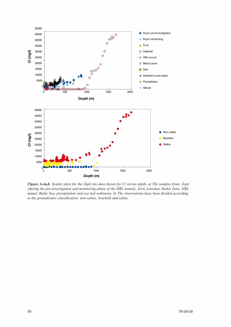
88 TR-09-09

Figure A-4a,b. Scatter plots for the Äspö site data shown for Cl versus depth. a) The samples from: Äspö (during the pre-investigation and monitoring phase of the HRL tunnel), Ävrö, Laxemar, Redox Zone, HRL tunnel, Baltic Sea, precipitation and sea bed sediments. b) The observations have been divided according to the groundwater classification: non-saline, brackish and saline.

0

5000

10000

15000

20000

25000

30000

35000

40000

45000

50000

0 500 1000 1500 2000

Depth (m)

Cl (

mg/

l)Äspö pre-investigation

Äspö monitoring

Ävrö

Laxemar

HRL tunnel

Redox zone

Sea

Sediment pore water

Precipitation

Glacial

0

5000

10000

15000

20000

25000

30000

35000

40000

45000

50000

0 500 1000 1500 2000

Depth (m)

Cl (m

g/l) Non saline

Brackish

Saline

TR-09-09 89

Figure A-5a. Scatter plots for the Äspö site data shown for Na, K and Ca versus the Cl concentration and depth. The observations have been divided according to the groundwater classification: non-saline, brackish and saline.

0100020003000400050006000700080009000

0 10000 20000 30000 40000 50000

Cl (mg/l)

Na (m

g/l)

0100020003000400050006000700080009000

0 500 1000 1500 2000

Depth (m)

Na (m

g/l)

020406080

100120140160180

0 10000 20000 30000 40000 50000

Cl (mg/l)

K (m

g/l)

020406080

100120140160180

0 500 1000 1500 2000

Depth (m)

K (m

g/l)

0

5000

10000

15000

20000

25000

0 10000 20000 30000 40000 50000

Cl (mg/l)

Ca (m

g/l)

0

5000

10000

15000

20000

25000

0 500 1000 1500 2000

Depth (m)

Ca (m

g/l)

Non saline Brackish Saline

90 TR-09-09

Figure A-5b. Scatter plots for the Äspö site data shown for Mg, HCO3 and SO4 versus the Cl concentration and depth. The observations have been divided according to the groundwater classification: non-saline, brackish and saline.

050

100150200250300350400

0 10000 20000 30000 40000 50000

Cl (mg/l)

Mg

(mg/

l)

050

100150200250300350400

0 500 1000 1500 2000

Depth (m)

Mg

(mg/

l)

0100200300400500600700800900

0 10000 20000 30000 40000 50000

Cl (mg/l)

0100200300400500600700800900

0 500 1000 1500 2000

Depth (m)

0

200

400

600

800

1000

1200

0 10000 20000 30000 40000 50000

Cl (mg/l)

0

200

400

600

800

1000

1200

0 500 1000 1500 2000

Depth (m)

Non saline Brackish Saline

SO

4 (m

g/l)

HCO

3 (m

g/l)

HCO

3 (m

g/l)

SO

4 (m

g/l)

TR-09-09 91

Figure A-5c. Scatter plots for the Äspö site data shown for tritium, δ2H and δ18O versus the Cl concentration and depth. The observations have been divided according to the groundwater classification: non-saline, brackish and saline.

0

20

40

60

80

100

0 10000 20000 30000 40000 50000

Cl (mg/l)

3 H (T

U)

0

20

40

60

80

100

0 500 1000 1500 2000

Depth (m)

3 H (T

U)-160-140-120-100-80-60-40-20

0

0 10000 20000 30000 40000 50000

Cl (mg/l)

2 H (S

MO

W)

-160-140-120-100-80-60-40-20

0

0 500 1000 1500 2000

Depth (m)

2 H (S

MO

W)

-25

-20

-15

-10

-5

0

0 10000 20000 30000 40000 50000

Cl (mg/l)

18O

(SM

OW

)

-25

-20

-15

-10

-5

0

0 500 1000 1500 2000

Depth (m)

18O

(SM

OW

)

Non saline Brackish Saline

92 TR-09-09

Depth (m) Water type Major ions Cl (mg/l) pH (units) Eh (mV)

0–100 Non-saline Na–Ca–K:HCO3–SO4–Cl <1,000 ∼ 6.5 ∼ –100100–350 Brackish Na–Ca–K: Cl–SO4–HCO3 1,000–5,000 ∼ 7.5 ∼ –200350–1,700 Saline Ca–Na–K:Cl– SO4–HCO3 >5,000 ∼ 8.5 ∼ –300

Figure A-6. Cl distribution at the Äspö site prior to (pre-investigation) and after the tunnel construction (monitoring). The major features of the non-saline, brackish and saline groundwaters are listed in the table above. The drawdown (80 m) of the groundwater surface, above the tunnel, is shown in the lower picture. The orientation of the cutting plane is N-S (see Figure A-1).

TR-09-09 93

When studying the major component chemistry the first working hypothesis was that: a) The groundwater evolution is fairly simple and can be described as following a two component evolu-tion path between non-saline and saline groundwaters; b) The system is stable and the HRL tunnel construction does not induce mixing between the non-saline and saline groundwaters to any large extentsincetheClstratificationisalmostunchanged;c)Thestabilityofthegroundwatersystemandalong term contact with the rock are generally regarded to result in water-rock interaction which is the major groundwater altering process. The working hypothesis had to be modified after a more careful examination of the groundwater data.

The depth stratification of groundwaters at the Äspö site is a result of the prevailing hydraulic forces, andthiscanbedepictedwhentheCl,Na,K,Ca,Mg,HCO3andSO4 are plotted versus depth. Highly salinegroundwaterscharacterisedbyahighCl,Na,K,Ca,MgandSO4contentandalowHCO3 andtritiumcontentcanbefoundwithin50mfromthebedrocksurfacedownto1,700mdepth.Incontrast,waterswitharecognisablenear-surfacecomponentsuchasalowCl,Na,K,Ca,MgandSO4contentbutahighHCO3andtritiumcontentcanbedetectedat900mdepth.

Amoredetailedevaluationoftheknowngroundwaterconservativetracerssuchasδ18OorδDshowedalowcorrelationwithCl(whenCl<10,000mg/l)whichindicatesamorecomplexsystem than first assumed (see Figure A-5c). The complexity increases further when considering that fast reactions such as bacteria mediated, ion-exchange, carbonate system and redox reactions can change the groundwater character relatively fast. Marine water may have undergone reactions such as ion-exchange with sea bed clay minerals outside the bedrock prior to entering the bedrock rather than reacting with the fracture clay minerals. Glacial water may have reacted eg, with pyrite in glacial sediments outside the bedrock. The slow reactions such as water-rock interaction with aluminium silicates may be a less important water modification. The relative low temperature of thegroundwaterinthebedrock,(at–200m=11°Cat–1,600m=33°C,thegradientis1.6°Cper100m)mayleadtothefactthatmanyofthereactionsneedmoretimethantheresidencetimeofthegroundwater/LaaksoharjuandWallin(eds)1997/.Iftransportprocessesandreactionstakingplaceoutside the bedrock are not compensated for, the mass balance calculations applied to groundwaters in the bedrock aquifer may be overestimated. The overestimation and the ambiguous groundwater data may lead to wrong assumptions concerning the residence time and, in the end, the stability and history of the groundwater.

A.3 Results of the M3 groundwater modellingA.3.1 Identified reference waters and end-membersGroundwaters used in the M3 modelling as a comparison to other groundwaters are by definition called reference waters. An end-member is a modelled water composition that is believed to be the original groundwater composition. It is important to note that all the available information such as δ14Cdatingδ34S and 36Cl(whereavailable)havebeenusedtocorrectlynamethereferencewatersand end-members. The end-member composition varies over time i.e. the meteoric water composi-tion has changed along an evolutionary line between the glacial end-member and modern precipita-tionduringthelast10,000years.Acommonfeaturefortheend-membersisthatthecompositionisuncertain due to assumed composition i.e. glacial melt water composition. In reality an end-member is not a fixed composition but only an extreme water which can change over time. The end-member water composition is important for understanding the origin of the water. The reference waters should be regarded as fixed points to which the observed groundwater composition is compared. The selected reference waters and the identified end-members are shown in the results from the principal componentanalysisinFigureA-7.Ifthemainpurposeistomodeltheevolutionandtominimiseuncertainty the reference water composition sampled in the rock rather than modelled end-member compositions should be utilised. The result of the modelling thus reflects mixing and reactions taking place in the bedrock which can explain the measured groundwater composition.

94 TR-09-09

ThereferencewatersforthecurrentmodellingshowninFigureA-7wereselectedsothatmostofthesampled Äspö site data can be described. In order to minimise the uncertainty only analysed samples of high quality were used. Too few or incorrect reference waters may lead to errors in the mixing and mass balance calculations and result in a misunderstanding of the processes. Most of the reference watersweresamplestakenintherockexceptfortheBalticreferencewater.Theselectedreferencewaters and end-members are:

• Brine reference waterwhichrepresentsthebrinetypeofwaterfoundinKLX02:1,631–1,681mwithameasuredClof47,200mg/l/Laaksoharjuetal.1995b/.BrinesarewaterswithsignificantlyhighersalinitythanOceanseawater.AttheÄspösitethelimitforBrinewassetto>40,000Cl,mg/l.Theinitialapproachwastoassumethatthedeepbrinegroundwaterin Laxemar was a totally closed two component system where diffusion was the dominating process. The Laxemar deepwaters were treated as a stagnant system in contact with the brackish groundwater systems rather than as a totally closed system. This contact may have taken place during the melting of the continental ice, natural influx or enhanced influx during drilling, hydrotesting or sampling. However, the samples at large depths have traces of tritium, indicating contactwiththeupperpartoftheaquifer/Laaksoharjuetal.1995b/.Thismaybeattributedtoacontamination of significantly younger waters in connection with the drilling operations.

• Glacial reference water which has been determined as a glacial water based on stable isotope valueswhichindicatecoldclimaterecharge(δ18O=–15.8SMOWandδ2H=–124.8SMOW)in combination with an apparent 14Cageof31,365years/SmellieandLaaksoharju1992/.ThistypeofwaterisfoundinÄspöKAS03:129–134m.Theglacialwaterisbelievedtohavebeeninjected into the basement during the melting and retreating of the continental ice sheet. These

Figure A-7. The M3 code was used to make a principal component plot based on the major components, stable isotopes and tritium values from the Äspö site. The selected reference waters to which all the other groundwater samples are compared are labelled. An end-member is a modelled water composition that is believed to be the original groundwater. A line is drawn between the reference waters so a polygon is formed. The polygon is used to define the observations for further modelling. The mixing ratios and the mass balances for the different observations are calculated. The weight for the different elements is shown in the equations for the first and second principal component respectively. These two principal components together account for 72% of the variability, or the information in the data.

-0.5

-0.4

-0.3

-0.2

-0.1

0

0.1

0.2

0.3

0.4

0.5

-0.7 -0.6 -0.5 -0.4 -0.3 -0.2 -0.1 0 0.1 0.2

L itor ina Sea

B altic Sea

Sedimentpor e water

A lter ed mar ine

M eteor ic

G lacial

B r ine

G lacial melt water

1960s Pr ecipitation

Subglacial?

C omponent 1 = - 0.25[Na] - 0.08[K ] - 0.23[C a] - 0.05[M g] + 0.11[H C O 3] - 0.24[C l] - 0.23[SO 4] + 0.08[3H ] - 0.03[2H ] + 0.01[18O ]

Com

pone

nt 2

= -

0.04

[Na]

- 0.

23[K

] +

0.05

[Ca]

- 0.

24[M

g] -

0.16

[HC

O3]

+ 0

.02[

Cl]

+ 0

.02[

SO4]

- 0

.10[

3H] -

0.2

7[2H

] - 0

.29[

18O

]

% of total varianceComp 1: 40%Comp 1+2: 72%

?

G r oundwater samples

Glacial

Äspö pre-investigation

Äspö monitoring

Ävrö

Laxemar

HRL tunnel

Redox zone

Sea

Sediment pore water

Precipitation

TR-09-09 95

meltwatershavemostlikelybeenmixedwithsalinegroundwatersresultinginnegativeδ18Osignatures of the water obtained. Glacial melt water can be observed at Äspö today at various depthsinthebasement/SmellieandLaaksoharju1992,WallinandPeterman1994/.TheGlacial melt water end-member is a modelled glacial melt water composition where the stable isotope values(δ18O=–21 SMOWandδ2H=–158SMOW)werebasedonmeasuredvalues(δ18O)inthe calcite surface deposits, and interpreted as sub-glacial precipitates, collected from different geological formations in Sweden. Some of the fracture fillings were assumed to be subglacial formations/TullborgandLarson1984/.Testsweremadeusingmanypossiblewatercompositionsfor the glacial water in order to select the composition that gave the best fit with the measured δ18Ocontentinthegroundwater.InordertosampleglacialmeltwaterasamplingcampaignwasperformedononeofthelargestglaciersinEuropecalledtheJosterdalsbreeninNorway.The glacier is situated in crystalline granitic bedrock and the main core of this glacier is up to 20,000yearsold.Samplesfromtheglaciericeweretakenandthemeltwaterstreamwassampledfor36kmdownstream/Laaksoharju1997/.

A modelled Subglacial water, in this case related to a possible water type formed below the continentaliceasaresultofelementconcentrationduetorepeatedfreezing,isshowninthePCA(FigureA-7).InordertodemonstratetheeffectoffreezingalaboratorytestwasconductedonthegroundwatersamplefromKAS03:129–134m.Theoriginalwaterhadachlorideconcentrationof1,220mg/l.A250mlsamplewasfrozenandthen,when50%oftheicefractionhadmelted,thechlorideconcentrationinthemeltwaterwas2,318mg/l.Theremainingicefractionwasmeltedseparatelyandthechlorideconcentrationinthismeltedwaterwas219mg/l.Thefreezinghadconcentratedthefirstfractionoftheoriginalwaterbyafactorof1.9(2,118/1,220mg/l).Thesecondfractionwasdiluted(comparedtotheoriginalwater)byafactorof5.6(1,220/219mg/l)/Laaksoharju1997/.Theassumedcompositionofthesubglacialgroundwaterwascalculatedfromthe difference between predicted and measured groundwater composition. This water composition couldexplainimportantdeviationsinconstituentssuchasSO4andCa.Butsincethiswatercomposi-tion is uncertain, further tests and investigations are needed before this water composition can be included as an end-member. In addition, the subglacial water composition most probably changed withtimeduringrepeatedfreezingandmeltingofthecontinentalicesheet.

• Baltic Sea reference waterwhichrepresentsmodernBalticSeawater.Theend-memberisLittorina SeawithaClconcentrationof6,100mg/lbasedonanalysesofmicrofossilsfromthemarinesedimentsinsouthernFinland/Kankainen1986/.BasedonmicrofossildeterminationinthesouthernpartoftheBalticSea,concentrationsupto14,000mg/lClhavebeensuggested/Winnetal.1988/.MixingportiontestswereperformedwherevariouspossibleLittorinaSeawaterconcentrationsweretested.Theformerconcentrationof6,100mg/lgavethebestfitwiththemeasuredClandδ18Ocontentinthegroundwater.TheLittorinaseahadahighersalinity(ofalmost a factor of two) compared to the selected reference water composition which was sample BalticSeawateroutsideÄspö.Furtherinvestigationsofthemicrofossilsinthemarinesedimentsaround Äspö could give new information concerning the local situation during the Littorina stage. The saline component in Littorina Sea water is ocean water.

• Altered marine reference waterwhichrepresentsBalticseawateralteredbybacterialsulphatereduction/Laaksoharjuetal.1995a/.ThiswatertypeisobtainedintheHRLtunnelbelowthe marine sediments. The end-member is the composition of the extracted marine sediment pore water. The stable isotopes were not measured for the pore water and a test was performed where the samples were given Littorina as well as modern values. The position of the samples inFigureA-7didnotchangeconsiderably.TheporewatercompositionresembledamoremodernBalticSeawatercompositionthanaLittorinaseawatercomposition.Inadditionthehydrogeologicalmodellingindicatedthatthemodernseacouldaffectthesediments.Basedonthis knowledge the modern isotope values were kept in the modelling. The origin and the isotopi-cal composition of microfossils of the sediments need further investigation. This information can be of great importance for the total postglacial scenario of the Äspö site.

• Meteoric reference waterwhichrepresentsadilute(Cl=5mg/l)non-salinewaterfoundinHBH02:7.5m.Theend-memberisanaverage1960 precipitation composition with a high tritium(100TU)content.ThisvalueisanestimatebasedonthemoderntritiumvaluesmeasuredatÄspöandtakingintoaccountthe12.43yearsofhalf-lifefortritium.Theprecipitationof1960couldcontainupto3,000tritiumunits/Alley1993/.

96 TR-09-09

A.3.2 Result of the mixing and mass balance modelling The results of the M3 modelling concerning the behaviour of the carbonate system in association with meteoric water at the Äspö site is described below. The complete modelling results are reported in/LaaksoharjuandWallin(eds)1997/.

Major element hydrochemistry as well as carbon and oxygen stable isotope data indicated large inputsofHCO3andbiogenicCO2(g)intheshallownon-salinegroundwatersatÄspö.ElevatedCO2 concentrationsinthegroundwater(6,050to15,037ppm)exceededatmosphericconcentrationsbyoneortwoordersofmagnitude.HighTOCvalues(upto20mg/l)andtheδ13CisotopevaluesoftheHCO3(–16to–14permillePDB)confirmedalargeuniformorganiccarbonsourceasoneend-memberforthecarbonsystem.Methane(1,030to4,070ppm)intheRedoxfracturezoneandtheshallowboreholeswithδ13Cvaluesbetween–39.8and–50.8o/oostronglysupportedabiogenicsource for this gas. The build-up of the bicarbonate reservoir most probably took place in the lower saturatedpartoftheshallowgroundwater(below30m).TheeffectofthisprocessasasourceofHCO3 can be seen in Figure A-8. Input of organic carbon with shallow groundwater provides a possible energy and carbon source for anaerobic respiration. The accelerated input of organic carbon added net reducing capacity to the groundwater that in turn prevented oxygen penetration. Reduction of iron(III) minerals to iron(II) in solution is an anaerobic process similar to sulphate reduction. This process was found to be the successor to the aerobic respiration of organic matter that was observed in the block scale Redox experiment. The process takes place when the amount of organic matter islargerthantheamountofdissolvedoxygen.Thisisroughlythecaseat>10mg/ltotalorganiccontent. A detailed description of the iron reduction is given in the reporting of the Redox project. Inorganicoxygenreductionwasexpected,butbiologicalconsumptionwasfound.OtherprocessesthatcanbeasourceforHCO3 are calcite solution, iron and manganese and sulphate reduction. The δ14CdatafromApril1995indicatedthatcalcitedissolutionismoreimportantinwaterswithshortresidence times while the biogenic input (slower process) completely dominates boreholes which

Figure A-8. Anaerobic respiration linked with organic decomposition is believed to be the major source for HCO3. The effect from the mixing portion of Meteoric water is shown in the background. The mixing por-tion is shown progressively: 0-20%, 20-40%, 40-60%, 60-80% and 80-100%. The weight for the different elements is shown in the equations for the first and second principal component respectively.

-0.5

-0.4

-0.3

-0.2

-1

0

0.1

0.2

0.3

0.4

0.5

-0.7 -0.6 -0.5 -0.4 -0.3 -0.2 -0.1 0 0.1 0.2

M eteor icmixing por tion

80 to 100%60 to 80%40 to 60%20 to 40%0 to 20%

L itor ina Sea

B altic Sea

Sedimentpor e water

A lter ed mar ine

M eteor ic

G lacial

B r ine

G lacial melt water

1960s Pr ecipitation

E nd-memberSample

Sour ces / Sink sH C O 3 (mg/l)

400 to 600

200 to 400

0 to 200

-200 to 0

-400 to -200

-600 to -400

C omponent 1 = - 0.25[Na] - 0.08[K ] - 0.23[C a] - 0.05[M g] + 0.11[H C O 3] - 0.24[C l] - 0.23[SO 4] + 0.08[3H ] - 0.03[2H ] + 0.01[18O ]

Com

pone

nt 2

= -

0.04

[Na]

- 0.

23[K

] + 0

.05[

Ca]

- 0.

24[M

g] -

0.1

6[H

CO

3] +

0.0

2[C

l] +

0.0

2[SO

4] -

0.10

[3H

] - 0

.27[

2H]

- 0.2

9[18

O]

% of total varianceComp 1: 40%Comp 1+2: 72%

TR-09-09 97

themselves are dominated by lateral flow. The calculations and the isotope data indicate that three carbon sources contribute to the dissolved bicarbonate /Tullborg and Gustafsson in Laaksoharju and Wallin(eds)1997/.TheseareinorganicCO2, anaerobic respiration and dissolution of calcite. Sinks forHCO3areoftenassociatedwithcalciteprecipitation.Evidencefromcarbonisotopegeochemistry/Wallin1993,Wallin1995,TullborgandGustafssoninLaaksoharjuandWallin(eds)1997/aswellasthemodellingoftheδ18Oandtritiumdatafromthegroundwaterinthefracturezonesuggestthatan extensive lateral flow of the water takes place. This, together with the decreasing chloride content over time, rules out the possibility of a large saline water component being mixed into the system.

3D visualisation of M3 calculationsThe result of the modelling can be used to visualise the origin and mixing behaviour of the groundwater at the site. The major reactions taking place in the bedrock were identified by means of M3 modelling in combination with standard geochemical modelling. The 3D interpolation of the M3mixingcalculationswereperformedbyusingINERGRAPH’sVoxelAnalystcomputercode.Theresultsofthemodellingareshownusinga2Dcuttingplane.ThelocationofthecuttingplaneisN-S,fororientationseeFigureA-1.TheobservationsusedinFigureA-9arecommonforthemodelusedinFigureA-6.Thehydraulictransmissivity/Rhén(ed)1997/ofthemajorfracturezonesisshownbasedonthecalculationsbeforedrawdown.Thetunnelconstructioncreateda–80mdrawdownofthegroundwatertablearoundtheelevatorshaft.ThisdrawdownisshowninFigureA-9.Thedrawdown resulted in changing inflow patterns and increased the mixing of different groundwater types. The short-term reactions listed in the Figures are believed to increase in intensity because of the increased flow associated with the drawdown.

Thenon-salinegroundwaterischaracterisedbyaNa–HCO3oraCa–HCO3 signature. The water is a result of infiltrated meteoric water that may have been mixed to some degree with brackish groundwater at different depths. Identified short-term fast reactions are redox reactions that hinder deepoxygenpenetrationintothebedrock.Oxygenconsumptionandcarbonateproductionlinkedtoorganic decomposition and iron reduction is the dominating redox reaction. Solution of calcite in the upper part of the bedrock and the resulting precipitation of calcite in the lower part of the bedrock can change the groundwater flow paths in fractured bedrock. Sinks and sources of anions and cations due to sorption/desorption (due to surface complexation and ion exchange) alter the water composi-tion of the non-saline groundwater.

FigureA-9showsadifferentpicturethanexpectedfromtheCldistributioninFigureA-6.ThisisduetothefactthatClisnotalwaysagoodtracerwhenitcomestofindingouttheevolution;neitherisitalwaysagoodindicatorofthedynamicsofagroundwatersystem.Forexample,theClconcentrationinFigureA-6showsminorchangesduringthetunnelconstructionaroundNE-1,themostconductivefracturezone.ThemixingproportionsinFigureA-9showmoredynamicchangesaroundthisfrac-turezone.TheClconcentrationisnotaffectedbyareplacementofwaterwithasimilarClcontentbut the change may be detected by integrating the information from several elements and isotopes thatmayhaveundergonemodifications.TheolderbrineandglacialwaterinNE-1isreplacedbymodernBalticseawaterandmodifiedmarinewater.TheincreasedmixingportionofmeteoricwaterinthedeeperpartofthisfracturezoneremainsundetectedwhenexaminingtheCldistribution.

A.3.3 Conclusions of the modellingThe findings and experiences from the M3 modelling at the Äspö site can be summarised accordingly:

The groundwater origin and evolution were described by means of mathematical models rather than by means of qualitative descriptions. Fundamental information for understanding the groundwater system was obtained after decoding the measured groundwater element concentration in terms of contributions from mixing and reactions.

Mixing is the dominating process affecting the groundwater composition.

A simple model eg, using one conservative tracer cannot be used to describe a complex natural system at the Äspö site without significant loss of information.

98 TR-09-09

Different elements and isotopes from the same water sample may contain different information concerningthegroundwaterevolutionhistory.ConservativenaturalgroundwatertracersCl,δ18Oandδ2H have several sources and origins.

Groundwater evolution models based on thermodynamic laws alone may not be applicable to a low temperature granitic groundwater system such as Äspö where equilibrium is not reached and where most of the reactions are biogenic.

Figure A-9. Proportion (%) of meteoric water at the Äspö island prior to and after tunnel construction calculated by using M3. The major reactions altering the groundwater are listed and the hydraulic trans-missivity of the major fracture zones are shown. The mixing proportions are always relative to the selected reference water composition. The orientation of the cutting plane is N-S (see Figure A-1).

Svensk Kärnbränslehantering ABSwedish Nuclear Fueland Waste Management Co

Box 250, SE-101 24 Stockholm Phone +46 8 459 84 00

Technical Report

TR-09-09

ISSN 1404-0344CM Gruppen AB, Bromma, 2009

M3 User’s Manual

Version 3.0

Marcus Laaksoharju, Geopoint AB

Erik Skårman, Abscondo

Javier Gómez

Geochemical modelling Group, University of Zaragoza

Ioana Gurban, 3D Terra

November 2009

TR-09

-09M

3 User’s M

anu

al - Versio

n 3.0